A Front-Tracking Method for Viscous, Incompressible, Multi ...
13
JOURNAL OF COMPUTATIONAL PHYSICS lo&2537 (1992) A Front-Tracking Method for Viscous, Incompressible, Multi-fluid Flows SALIH OZEN UNVERDI AND G&TAR TRYGGVASON Department of Mechanical Engineering and Applied Mechanics, The University of Michigan, Ann Arbor, Michigan 48109 Received July 5, 1990; revised May 10, 1991 A method to simulate unsteady multi-fluid flows in which a sharp interface or a front separates incompressible fluids of different density and viscosity is described. The flow field is discretized by a conservative finite difference approximation on a stationary grid, and the interface is explicitly represented by a separate, unstructured grid that moves through the stationary grid. Since the interface deforms continuously, it is necessary to restructure its grid as the calculations proceed. In addi- tion to keeping the density and viscosity stratification sharp, the tracked interface provides a natural way to include surface tension effects. Both two- and three-dimensional, full numerical simulations of bubble motion are presented. 0 1992 Academic Press. Inc 1. INTRODUCTION Accurate simulation of fluid flow with a sharp front presents a problem of considerable difficulty which has challenged inventors and users of numerical methods since the beginning of large-scale computational work. Fronts or interfaces occur commonly in fluid mechanics problems. Shocks in compressible flows, vortex sheets in inviscid flows, and boundaries between immiscible fluids are some of the better known examples. In principle, all of these problems can be handled numerically by working with the governing equations in integral form, which lead to conser- vative finite difference schemes and thus avoid any assump- tions about the differentiability of the solution. In practice, however, straightforward application of a conservative schemeis severely limited when a sharp interface is present. If the numerical method is of a low order, excessive numeri- cal diffusion will quickly destroy the sharpnessof the front; a higher order scheme will lead to numerical oscillations around the front that may couple into other parts of the solution in an undesirable way. Here, we present a method for incompressible flows of two or more immiscible fluids where the interface is explicitly tracked to keep the density and viscosity fields sharp and to allow the inclusion of sur- face tension forces at the interface. The method has been implemented for both two- and three-dimensional flows. Basically, two strategies exist to deal with flows con- taining sharp fronts. In front-capturing, the basic approach is to use a finite volume discretization of the whole domain, while modifying the numerical approximation to minimize numerical difficulties. This generally involves using a high (usually second) order scheme and adding artificial viscosity around the front to diffuse it slightly to avoid oscillations. The fundamental idea goes back to von Neumann and Richtmayer. Since then shock-capturing has become considerably more sophisticated because of the introduction of schemes that explicitly enforce monotonicity through a nonlinear step and at the sametime maintain high order “almost everywhere.” These methods (see, e.g., Boris [7] for a review) generally serve well for shocks but work lesswell for contact discontinuity. Further- more, relatively fine grids are still needed,thus limiting most unsteady flow simulations to two dimensions. An alternative to front-capturing is tracking, where addi- tional computational elements are introduced explicitly to keep track of the front. This generally reduces by a considerable amount the resolution needed to keep the front sharp, and eliminates numerical diffusion altogether. However, tracking is best suited for well-defined fronts that are easily identifiable in the initial conditions. Tracking methods can be divided further into volume- tracking and front-tracking. In volume-tracking methods a marker, used to reconstruct the interface, is advected with the flow. In the well-known marker-and-cell (MAC) method of Harlow and Welch [25], marker particles were inserted to identify the spatial region occupied by a single fluid with a free surface. Daly [15] relined this method to allow it to deal with two fluid problems. Other extensions and refinements can be found in Daly [16] and Amsden and Harlow [3], for example. Hirt and Nichols [26] abandoned the use of marker particles and instead used a marker function advected by the flow. At each time step they reconstructed the front from the marker function by generating either a horizontal or a vertical interface within each interface cell. This interface was then advected with 25 0021-9991/92 $5.00 Copyright 0 1992 by Academic Press, Inc. All rights of reproduction in any form reserved.
Transcript of A Front-Tracking Method for Viscous, Incompressible, Multi ...
JOURNAL OF COMPUTATIONAL PHYSICS lo&2537 (1992)
A Front-Tracking Method for Viscous, Incompressible, Multi-fluid Flows
SALIH OZEN UNVERDI AND G&TAR TRYGGVASON
Department of Mechanical Engineering and Applied Mechanics, The University of Michigan, Ann Arbor, Michigan 48109
Received July 5, 1990; revised May 10, 1991
A method to simulate unsteady multi-fluid flows in which a sharp interface or a front separates incompressible fluids of different density and viscosity is described. The flow field is discretized by a conservative finite difference approximation on a stationary grid, and the interface is explicitly represented by a separate, unstructured grid that moves through the stationary grid. Since the interface deforms continuously, it is necessary to restructure its grid as the calculations proceed. In addi- tion to keeping the density and viscosity stratification sharp, the tracked interface provides a natural way to include surface tension effects. Both two- and three-dimensional, full numerical simulations of bubble motion are presented. 0 1992 Academic Press. Inc
1. INTRODUCTION
Accurate simulation of fluid flow with a sharp front presents a problem of considerable difficulty which has challenged inventors and users of numerical methods since the beginning of large-scale computational work. Fronts or interfaces occur commonly in fluid mechanics problems. Shocks in compressible flows, vortex sheets in inviscid flows, and boundaries between immiscible fluids are some of the better known examples. In principle, all of these problems can be handled numerically by working with the governing equations in integral form, which lead to conser- vative finite difference schemes and thus avoid any assump- tions about the differentiability of the solution. In practice, however, straightforward application of a conservative scheme is severely limited when a sharp interface is present. If the numerical method is of a low order, excessive numeri- cal diffusion will quickly destroy the sharpness of the front; a higher order scheme will lead to numerical oscillations around the front that may couple into other parts of the solution in an undesirable way. Here, we present a method for incompressible flows of two or more immiscible fluids where the interface is explicitly tracked to keep the density and viscosity fields sharp and to allow the inclusion of sur- face tension forces at the interface. The method has been implemented for both two- and three-dimensional flows.
Basically, two strategies exist to deal with flows con- taining sharp fronts. In front-capturing, the basic approach is to use a finite volume discretization of the whole domain, while modifying the numerical approximation to minimize numerical difficulties. This generally involves using a high (usually second) order scheme and adding artificial viscosity around the front to diffuse it slightly to avoid oscillations. The fundamental idea goes back to von Neumann and Richtmayer. Since then shock-capturing has become considerably more sophisticated because of the introduction of schemes that explicitly enforce monotonicity through a nonlinear step and at the same time maintain high order “almost everywhere.” These methods (see, e.g., Boris [7] for a review) generally serve well for shocks but work less well for contact discontinuity. Further- more, relatively fine grids are still needed, thus limiting most unsteady flow simulations to two dimensions.
An alternative to front-capturing is tracking, where addi- tional computational elements are introduced explicitly to keep track of the front. This generally reduces by a considerable amount the resolution needed to keep the front sharp, and eliminates numerical diffusion altogether. However, tracking is best suited for well-defined fronts that are easily identifiable in the initial conditions.
Tracking methods can be divided further into volume- tracking and front-tracking. In volume-tracking methods a marker, used to reconstruct the interface, is advected with the flow. In the well-known marker-and-cell (MAC) method of Harlow and Welch [25], marker particles were inserted to identify the spatial region occupied by a single fluid with a free surface. Daly [15] relined this method to allow it to deal with two fluid problems. Other extensions and refinements can be found in Daly [16] and Amsden and Harlow [3], for example. Hirt and Nichols [26] abandoned the use of marker particles and instead used a marker function advected by the flow. At each time step they reconstructed the front from the marker function by generating either a horizontal or a vertical interface within each interface cell. This interface was then advected with
25 0021-9991/92 $5.00
Copyright 0 1992 by Academic Press, Inc. All rights of reproduction in any form reserved.
26 UNVERDI AND TRYGGVASON
its normal velocity to update the marker function. Later developments include the simple line interface calculations (SLIC) of Noh and Woodward [33] and refinements by Chorin [lo] and others.
Volume-tracking methods enjoy considerable popularity because they are reasonably accurate and relatively simple to implement. For higher accuracy at the cost of con- siderably more complexity, it is necessary to use front- tracking, where the interface itself is described by additional computational elements. The basic idea is discussed by Richtmyer and Morton [39], but its primary implementa- tion has been through the work of J. Glimm and coworkers (see, e.g., Glimm, Grove, Lindquist, McBryan, and Tryggvason [24]). They represent the moving front by a connected set of points, which forms a moving internal boundary. To calculate the evolution inside the fluid in the vicinity of the interface, an irregular grid is constructed and a special finite difference stencil is used on these irregular grids. Several problems have been addressed by this method, notably compressible flows of stratified fluids (e.g., Chern, Glimm, McBryan, Plohr, and Yaniv [S]) and the motion of saturation fronts in porous medium (e.g., Daripa, Glimm, Lindquist, Maesumi, and McBryan [ 171). For aerodynamics calculations with another front-tracking method see the review by Moretti [31]. A front-tracking technique based on a somewhat different idea than those described above has been developed by Peskin and collaborators (see e.g., Peskin, [35]; Fauci and Peskin, [19]; Fogelson and Peskin, [20]). In this work, which is limited to incompressible and homogeneous fluids, the interface is again represented by a connected set of particles which carry forces, either imposed externally or adjusted in such a way as to achieve a specific velocity at the interface. In this case, however, the fixed grid is kept unchanged, even near the interface, and the interface force is simply distributed onto the fixed grid.
The major drawback of direct front-tracking is its com- plexity. In addition to the obvious question of how the inter- face grid interacts with the stationary grid, and vice versa, it is generally necessary to restructure the interface grid dynamically as the calculations proceed. Computational points must be added in regions where the grid stretches, and usually it is desirable to eliminate points from regions of compression. Additional complications, to be discussed later, arise in three dimensions. Another major problem for front-tracking results from the interaction of a front with another front (or another part of the same front). Generally, the computational procedure does not recognize more than one front in each cell of the stationary grid, and therefore double interfaces have to be merged into one interface or eliminated. A merging algorithm that has been used with some success in two-dimensional simulations is described by Glimm, Grove, Lindquist, McBryan, and Tryggvason [ 241.
Several specialized methods for flows that can be treated either as inviscid, or that are so viscous that inertial force5 may be neglected (Stokes flows), are properly classified as front-tracking methods. In these cases the governing equa- tions can be reformulated as an integral equation over the moving boundaries and interfaces so the only grid is the front grid. These methods are generally referred to as boundary integral, or boundary element methods, but vor- tex methods for generalized vortex sheets also belong to this class. Although it is usually highly desirable to reformulate a problem as an integral equation, occasionally it is more efficient to retain an Eulerian grid for part of the calculation, The well-known vortex-in-cell (VIC) method is such a hybrid, where the vorticity is carried by distinct Lagrangian particles, but a stationary Eulerian grid is used to find the velocities. In its original form the VIC method was developed for homogeneous fluids, but extensions to weakly stratified flows were devised by Meng and Thomson [30] and by Tryggvason [47] for arbitrary stratification.
In this article we present a front-tracking method for incompressible, viscous, multi-fluid flows. While the inter- face is explicitly tracked, it is not kept completely sharp but is rather given a finite thickness of the order of the mesh size to provide stability and smoothness. This thickness remains constant for all time (no “numerical diffusion”) but decreases with liner resolution of the stationary grid. Since the fluids are incompressible, the interface simply moves with the fluid velocity, which is interpolated from the grid. The method incorporates some of the features of volume- tracking and shock-capturing schemes in that the original underlying grid is retained through the simulations and no restructuring is needed to align the grid with the interface. However, the interface is explicitly tracked, as in the front- tracking method of Glimm and coworkers (e.g., Glimm et al. [23]), and like methods based on moving grids, such as the one discussed in Fritts and Boris [21] and Fyfe, Oran, and Fritts [22]. When the method is described in detail, it becomes clear that it is actually most related to the VTC method and Peskin’s method. Its major differences are that the tracked interfaces carry the jump (or gradient) in properties across the interface and that, at each time step, the property field is reconstructed by solving a Poisson equation (using a fast solver). The primary advantage of this approach is that interfaces can interact in a rather natural way, since the gradients simply’add or cancel as the grid distribution is constructed from the information carried by the tracked front. This interaction-automatically taken care of in our method-is considered one of the great dif- ficulties of front-tracking methods and one of the reasons that volume-tracking methods have been favored in the past (see, e.g., Hirt and Nichols, [26]; Hyman, [27]; Oran and Boris, [34]; Floryan and Rasmussen, [IS]).
The rest of the paper is arranged as follows: A short over- view of previous numerical calculations of bubble motion
VISCOUS, MULTI-FLUID FLOWS 21
is given in Section 2. Section 3 discusses the numerical method. Since the finite difference method is a conventional one, we only describe it briefly and focus instead on the front-tracking part. In Section 4 we present several sample calculations of bubbles rising in a gravity field, both for a two- and a three-dimensional flow. Our conclusions appear in Section 5. A short account of some of the work reported here was presented at the Annual Meeting of the Division of Fluid Dynamics of the American Physical Society at Ames, CA, November 19-21, 1989, and at the regional meeting of the American Mathematical Society in Manhattan, KS, March 16-17, 1990. Calculations of the evolution of a three- dimensional, weakly stratified Rayleigh-Taylor instability with a preliminary version of our front-tracking scheme appeared in Tryggvason and Unverdi [48].
2. BACKGROUND
In order to demonstrate its capabilities, we have used our method to simulate the motion of bubbles. To put this work into proper perspective, a short overview of previous bubble simulations follows. Several investigators have applied boundary integral techniques to predict the deformation of drops and bubbles at zero Reynolds number (Stokes flow) in a strain field. Youngren and Acrivos [SO] considered a gas bubble in viscous extensional flow, and Rallison [37] considered the time-dependent deformation of a drop with a viscosity equal to the surrounding fluid in the only fully three-dimensional calculation so far. More recent work includes Stone and Leal’s [44] study of the breakup of extended drops, and investigations of the deformation of an initially non-spherical drop in the Stokes limit by Koh and Lea1 [28] and Pozrikidis [36]. The last study shows that the spherically shaped solution of Hadamart (see, e.g., Clift, Grace, and Weber [ 133 ) is indeed very stable, while the relaxation of a non-spherical drop toward a spherical shape includes some rather remarkable processes, including the shedding of the fluid in the drop and, in other cases, ingestion of the outer fluid. For recent experiments on the breakup of drops in simple flow fields, see Stone, Bentley, and Lea1 [43]. A thorough review of the deformation of small drops and bubbles in viscous flows and a list of other contributions has been given by Rallison [38] and Acrivos [ 11. Other computations using the Stokes flow approxima- tion include, for example, a study of the axisymmetric motion of a viscous drop toward a fluid interface for a range of capillary numbers and viscosity ratios by Chi and Lea1 [9], simulation of the formation of two-dimensional drops due to a Rayleigh-Taylor instability in a thin viscous film for fluids of equal viscosities by Yiantsios and Higgins [Sl 1, and an investigation of the motion of drops through circular tubes by Martinez and Udell [29]. Computations of the breakup of contaminated drops in a strain field are reported by Stone and Lea1 [45].
For bubbles rising due to buoyancy, inertial effects are often of great importance, and bubble deformation can be considerable. Ryskin and Lea1 [4&42] examined the steady-state shape of a number of rising axisymmetric bubbles using a finite difference technique and a boundary- fitted coordinate system. They also applied their numerical technique to an investigation of the steady-state shape of bubbles in an axisymmetric strain flow. More recently Dandy and Lea1 [ 143 extended this method to the two-fluid problem, where the bubble is assumed to have finite density and viscosity. Unsteady numerical calculations of the initial deformation of two-dimensional, inviscid, bubbles include those done by Anderson [2] in the case where the density ratio is very small and Baker and Moore [4] in the case of a bubble of zero density. Other unsteady, two-dimensional flow calculations around deformable drops have been presented by Fyfe, Oran, and Fritts [22], who used a moving triangular grid. Calculations of inviscid, fully three- dimensional bubbles, for weak stratification and excluding surface tension, were presented by Brecht and Ferrante [6].
The above numerical studies, as well as a large number of experimental investigations, have led to a reasonably good understanding of the motion of a single buoyant bubble. A summary and graphic representation of the various rise modes can be found in Clift, Grace, and Weber [13] and Churchill [12], for example. Bubbles can be characterized by the Morton number, M= gpz/p,o’, and the Eotvos number, Eo = p,gdz/a (also called the Bond number), as well as by their density, pb/pO, and viscosity, pb/p,, ratios. Here the subscript o refers to the outer fluid, b to the bubble fluid, p is the viscosity, p the density, c the surface tension, g the gravity acceleration, and d, the “effec- tive” diameter of the bubble. The Morton number involves the fluid properties only, and the Eotvos number is the non- dimensional size of the bubble. The rate of rise is expressed as a Reynolds number in terms of the rise velocity, Re = pUdJp, where U is the velocity. Often the Weber num- ber, We = pU2dJo, is also used to characterize the bubble. Obviously Eo and M are the parameters that one actually controls. Re and We are found only after the terminal velocity has been determined. For all M, sufficiently small bubbles remain spherical and rise in a steady-state way. Likewise, large enough bubbles become a “spherical cap” and rise in a steady-state fashion. In the transition zone from small to large bubbles, the motion depends on the Morton number of the liquid. Bubbles in high M fluids become ellipsoidal (or “dimpled ellipsoidal-cap” for even larger M) before turning into a spherical cap shape, but continue to have a well-defined steady-state motion. For low M liquids, like water, while the bubbles also become ellipsoidal, their motion is unsteady, following a zigzag or helical path. One they become a spherical cap and resume steady-state motion, their wake is usually turbulent for high Re. While ellipsoidal bubbles are usually spherical on top,

28 UNVERDI AND TRYGGVASON
and flatter on the bottom, Ryskin and Lea1 [41], in their numerical study, found bubbles with a relatively flat top and more spherical back, for low viscosity outer fluid.
3. NUMERICAL METHOD
The equations governing the motion of unsteady, viscous, incompressible, immiscible two-fluid systems are the Navier-Stokes equations. In conservative form these are
= -Vp+pg+V.(2pD)+a~n&x-x~~). (1)
Here u is the velocity field; p and p are the discontinuous density and viscosity fields, respectively. D is the rate of deformation tensor, whose components are D,= &(ui, j + u~,~), 0 is the surface tension coefficient, K is the curvature, and n is a normal to the interface separating the two fluids. 6(x-x1) is a delta function that is zero everywhere except at the interface, where x = x’; g is the gravity force.
These are supplemented by the incompressibility condi- tion
v.u=o (2)
and equations of state for the density and the viscosity. Here the density and viscosity fields of a material particle remain constant, so the equations of state are simply
s+u.vp=o, ap t+u.vp=o. (3)
Inside each fluid, p and p are constants. The above equations are solved in a rectangular two- and
three-dimensional domain with a finite difference method, conventional in every way except that the advection of the density and the viscosity fields is achieved by explicit tracking of the interface between the two fluids, instead of solving Eq. (3) directly. The spatial differentiation is calculated by second-order finite differences on a staggered Eulerian grid, and the time advection is either by a simple, explicit Euler method, or, for some of the two-dimensional calculations, by a second order Adams-Bashforth method. When the Euler time integration method is used, the finite difference approximation is exactly the same as in the MAC method. The boundary conditions on our computational domain are either periodic or full slip in the horizontal directions and a rigid, stress-free top and bottom. The general setup of our problem is sketched in Fig. 1.
Combining the incompressibility condition and the momentum equations results in a nonseparable, elliptic
FIG. 1. The computational setup. The computational domain is discretized by a regular, three-dimensional, Cartesian, stationary grid. The front is represented by a separate unstructured, two-dimensional, triangular grid. The computations are done in a box with rigid (full slip) top and bottom and full slip or periodic boundaries in the horizontal direction.
equation for the pressure. This equation is solved by a mul- tigrid method (MGD described in Wesseling [49]) in two- dimensions, while a simple, two-color, successive over- relaxation scheme is used for the three-dimensional runs.
The major novelty of the method described here is the way p and p are updated. Since these variables are both discontinuous across the interface, we may expect either excessive numerical diffusion or problems with oscillations around the jump if no special treatment is used at the front. To avoid these problems we introduce an additional computational element-the interface grid-that explicitly marks the position of the interface. An indicator funcion, Z(x), that is 1 inside the bubble and 0 in the outer fluid, is then constructed from the known position of the interface. Since p and p are constant within each fluid, this indicator function allows us to evaluate the proper values of these variables at each grid point by
P(X) = PO + (PI3 - PO) Z(x)
P(X) = PO + (Pb - PO) Z(x). (4)
To avoid introducing disturbances of length scale equal to the mesh by having the properties jump abruptly from one grid point to the next, the interface is not kept completely sharp but given a small thickness of the order of the mesh size. In this transition zone the fluid properties change smoothly from the value on one side of the interface to the value on the other side. This artificial interface thickness is a function of the mesh size used, only, and does not change during the calculations. Therefore no numerical diffusion is present. This finite thickness also serves to position the
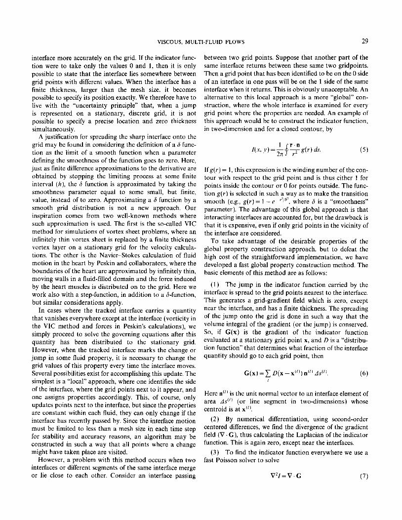
VISCOUS, MULTI-FLUID FLOWS 29
interface more accurately on the grid. If the indicator func- tion were to take only the values 0 and 1, then it is only possible to state that the interface lies somewhere between grid points with different values. When the interface has a finite thickness, larger than the mesh size, it becomes possible to specify its position exactly. We therefore have to live with the “uncertainty principle” that, when a jump is represented on a stationary, discrete grid, it is not possible to specify a precise location and zero thickness simultaneously.
A justification for spreading the sharp interface onto the grid may be found in considering the definition of a 6 func- tion as the limit of a smooth function when a parameter defining the smoothness of the function goes to zero. Here, just as finite difference approximations to the derivative are obtained by stopping the limiting process at some finite interval (h), the 6 function is approximated by taking the smoothness parameter equal to some small, but finite, value, instead of to zero. Approximating a 6 function by a smooth grid distribution is not a new approach. Our inspiration comes from two well-known methods where such approximation is used. The first is the so-called VIC method for simulations of vortex sheet problems, where an infinitely thin vortex sheet is replaced by a finite thickness vortex layer on a stationary grid for the velocity calcula- tions. The other is the Navier-Stokes calculation of fluid motion in the heart by Peskin and collaborators, where the boundaries of the heart are approximated by infinitely thin, moving walls in a fluid-filled domain and the force induced by the heart muscles is distributed on to the grid. Here we work also with a step-function, in addition to a b-function, but similar considerations apply.
In cases where the tracked interface carries a quantity that vanishes everywhere except at the interface (vorticity in the VIC method and forces in Peskin’s calculations), we simply proceed to solve the governing equations after this quantity has been distributed to the stationary grid. However, when the tracked interface marks the change or jump in some fluid property, it is necessary to change the grid values of this property every time the interface moves. Several possibilities exist for accomplishing this update. The simplest is a “local” approach, where one identifies the side of the interface, where the grid points next to it appear, and one assigns properties accordingly. This, of course, only updates points next to the interface, but since the properties are constant within each fluid, they can only change if the interface has recently passed by. Since the interface motion must be limited to less than a mesh size in each time step for stability and accuracy reasons, an algorithm may be constructed in such a way that all points where a change might have taken place are visited.
However, a problem with this method occurs when two interfaces or different segments of the same interface merge or lie close to each other. Consider an interface passing
between two grid points. Suppose that another part of the same interface returns between these same two gridpoints. Then a grid point that has been identified to be on the 0 side of an interface in one pass will be on the 1 side of the same interface when it returns. This is obviously unacceptable. An alternative to this local approach is a more “global” con- struction, where the whole interface is examined for every grid point where the properties are needed. An example of this approach would be to construct the indicator function, in two-dimension and for a closed contour, by
If g(r) = 1, this expression is the winding number of the con- tour with respect to the grid point and is thus either 1 for points inside the contour or 0 for points outside. The func- tion g(r) is selected in such a way as to make the transition smooth (e.g., g(r) = 1 - ~~r2’sZ, where 6 is a “smoothness” parameter). The advantage of this global approach is that interacting interfaces are accounted for, but the drawback is that it is expensive, even if only grid points in the vicinity of the interface are considered.
To take advantage of the desirable properties of the global property construction approach, but to defeat the high cost of the straightforward implementation, we have developed a fast global property construction method. The basic elements of this method are as follows:
(1) The jump in the indicator function carried by the interface is spread to the grid points nearest to the interface. This generates a grid-gradient field which is zero, except near the interface, and has a finite thickness. The spreading of the jump onto the grid is done in such a way that the volume integral of the gradient (or the jump) is conserved. So, if G(x) is the gradient of the indicator function evaluated at a stationary grid point x, and D is a “distribu- tion function” that determines what fraction of the interface quantity should go to each grid point, then
G(x) = c D(x -xc’)) n(l) Ad’).
Here n(‘) is the unit normal vector to an interface element of area ds”’ ( or 1’ me segment in two-dimensions) whose centroid is at x(I).
(2) By numerical differentiation, using second-order centered differences, we find the divergence of the gradient field (V . G), thus calculating the Laplacian of the indicator function. This is again zero, except near the interfaces.
(3) To find the indicator function everywhere we use a fast Poisson solver to solve
V21=V.G (7)

30 UNVERDI AND TRYGGVASON
with the proper boundary conditions. Here the right-hand side is calculated in (1) and (2). The Laplacian is approximated by the standard second-order, finite difference approximation.
This approach leads to a field quantity Z(x), which is con- stant within each fluid, but has a finite thickness transition zone around the interface and therefore approximates a two-dimensional step-function. Obviously the method extends easily to problems where there are more than two fluids present.
In the calculations reported here we have used the distribution function
D(x - .(‘I) = (4h)-’ fi (
i= I 1 +cos; (x;-xxj’)) ,
> if ~x~-x;‘)/ <2h, i= 1, cc;
otherwise, (8)
introduced by Peskin [35]. Here h is the Eulerian mesh width and c( = 2, 3 (two- and three-dimensions, respec- tively). This function has several desirable properties, as dis- cussed by Peskin [35]. We have also experimented with a simpler area-weighting distribution as frequently used in VIC calculations (see, e.g., Christiansen [ 111). This gives a sharper interface, but not quite as smooth a transition. The area weighting distribution is obviously much simpler than (8) but is known to introduce small-scale anisotropy (e.g., Tryggvason [47]). We have not yet conducted a detailed investigation of under what circumstances such anisotropy can be tolerated, but it is likely that when surface tension is important small scale smoothness is desirable.
In those calculations where surface tension is included we find the magnitude of the surface tension force from the curvature of the interface:
Here 0 is the surface tension coefficient, and K(‘) is the curvature of the interface at the centroid of element (I). This force is then distributed onto the grid in the same way as the gradient, thus constructing a grid-force field
F(x) = 1 D(x - xc’)) f (‘). (10)
This ensures that the total force is conserved when going from the interface to the grid. The distributed surface tension force gives a body-force-like term in the equations of motion, and this term is included in calculation of the velocity field. Its divergence also appears in the source term for the pressure equation.
To interpolate the velocities of the interface points from the grid velocities we use the same gridpoints that the
gradient was distributed to and the same weight functions. The velocity at interface point 1 is, therefore,
UC’) = 1 qxi- .(‘)) u,, (11)
where the sum is over the points on the stationary grid in the vicinity of the interface point. The interface is then advected by integrating
dx”‘= uu,, dt (121
Discrete points on the interface are advected with the flow and the interface itself is formed by connecting these points. In two dimensions, two points are connected by a straight line segment, but in three dimensions, three points are connected by a triangular element. The data structure is therefore the same as is commonly used in finite element modeling, which makes the use of graphics tools developed to visualize such models convenient. (The three-dimen- sional figures in this paper were generated by the Applica- tion Visualization System software on a Stellar work- station.)
As the interface deforms, some parts of it are depleted of computational points, and other parts may become crowded with points. To maintain an adequate resolution, we must add computational elements as the interface stretches and (although often not necessary) remove elements that become very small. In two dimensions, where the front is simply a line, these modifications are a relatively simple matter. The distance between two markers is kept within a lower bound and an upper bound by adding and deleting points. When the interface is a surface embedded in a three- dimensional flow, this aspect literally takes on a whole new dimension. Our regridding procedure consists of three basic steps: (1) node addition (for elements that become too large); (2) node deletion (when elements become small); and (3) reconnection or restructuring (to eliminate bad “aspect ratios, ” i.e., elements that have a small area but a large perimeter). Restructuring is sometimes also needed for three-dimensional surfaces to improve their smoothness. Figure 2 depicts these three basic regridding operations schematically. (For a discussion of these problems for two- dimensional simulations on a moving triangular grid see, e.g., Fritts and Boris [21].)
For the calculation of interface curvature we have implemented somewhat different methods for the two- dimensional and the three-dimensional calculations. In two dimensions we lit a local, cubic, Hermite polynomial to four points on the interface and find the curvature by differentia- tion with respect to the arc length. The surface tension force is found by evaluating the curvature at the middle of the element. To calculate the mean curvature of an interface

VISCOUS, MULTI-FLUID FLOWS 31
(b’ @ r) @
FIG. 2. The basic operations in dynamic restructuring of the three- dimensional interface grid: (a) addition of a point by bisection of the longest side of a large element; (b) point deletion to eliminate small elements and remove points; (c) reconnection to eliminate elements with large perimeter and small area.
in three dimensions we use a method described by Todd and McLeod [46]. At each point on the interface grid we identify its neighbors. By fitting circles through the point of interest and neighboring points, two at a time, we obtain a set of tangent vectors and curvatures. The normal is found by averaging the vector product of the various tangent vectors. This information is then used to estimate the coefficients in the so-called Dupin indicatrix by a least squares method. These coefficients give the mean curvature, in, directly. Multiplying the average of the mean curvature vector at the three vertices of each triangular element by the surface tension coefficient and the area of the element, CJ AA, gives the resultant surface tension force on the element. Dis- tribution of this force onto the grid by the three-dimensional distribution function completes the interaction of the interface and the Eulerian grid. In addition to calculations of surface tension forces, the curvature is needed when interface points are added.
4. COMPUTATIONAL EXAMPLES
A preliminary version of the method described above has been used to study the Rayleigh-Taylor instability of two fluids of similar density, where the Boussinesq approxima- tion is applicable. The Boussinesq approximation leads to a separable pressure equation and hence simplifies the calculations considerably. These calculations, reported in Tryggvason and Unverdi [48], included neither surface tension nor dynamic restructuring of the interface mesh. Here, we present calculations of buoyant bubbles, both in two and three dimensions where the fluids can have arbitrary density difference, surface tension is included, and
the interface grid is restructured to allow long time simula- tions.
A number of bubbles for various Eo and M are shown in Fig. 3. The figure demonstrates the (essentially) steady states, but in each case the full unsteady problem is solved. The physical times are equal for each row, but the middle and bottom row are at twice the time of the top row. These calculations are all done on a 65 by 129 grid, and the com- putational box has rigid, full slip boundaries. Therefore, considerable boundary effects may be expected. Here, p,,/pb = 40, and the Eiitvijs number, the Morton number, and the viscosity ratio for each frame are noted in the caption. For small Eo (i.e., large surface tension or small bubble), the bubbles remain nearly circular, but for higher Eo the bubbles attain a steady state with a somewhat flat or
0 I (a)
(e)
0
(b)
(f)
a
(i) Cj) Ik)
1
(d)
0
(h)
(I)
FIG. 3. The steady-state rise of a rising bubble for various Eo and M. Here po/pb=40. Top row, Eo= 1; M= IO-‘; 10e6; 10e5; lo-“; p0/pb=88; 156; 277; 493. Middle row, Eo= 10; M= 10m4; 10m3; IO-*; 10-i; pO/pb = 88; 156; 277; 493. Bottom row, Eo = 104; M= 10-l; 1; 10; 102;po/pb=85; 151;269;479.

32 UNVERDI AND TRYCGVASON
(a) (b) (d)
(e) (f) (g) (h)
FIG. 4. The stream lines for the top and the middle frames in Fig. 3.
elliptic shape. Even higher Eo results in bubbles with a nearly flat back and semicircular front. For low Eo and M (low viscosity but high surface tension or small bubble, i.e., the top left frame), this latter shape is actually inverted with the top being slightly flatter than the back. This agrees with Ryskin and Leal’s [41] prediction for steady-state axisym- metric bubbles. For the highest Eo and lowest M (lower left- hand corner), the solution shown is not truly a steady state;
the skirts pulled off the bubble with the separated flow increase continuously in length. At the highest Eotvos number (bottom row) the position of the bubble is relatively independent of the Morton number, but for the lowest Eo a strong dependency is observable. This is as we would expect. Low Eo corresponds to small bubbles where viscous drag is important; for larger bubbles (and Eo) the drag is mostly pressure drag and the velocity is therefore relatively independent of the viscosity.
To examine the flow field around the bubbles in more detail, we plot the stream lines in Fig. 4 in a frame of reference moving with the bubble for the bubbles in Figs. 3a through h. For high Morton numbers (and therefore low Reynolds numbers), the flow around the bubble is nearly a Stokes flow. No wake is visible behind the bubble, and the interior of the bubble consists of a single vortex pair. As the Morton number decreases, the Reynolds number increases and a wake appears behind the bubble. For small Eo, where the bubbles remain nearly circular, the wake is relatively small, but as the bubble deforms more, a larger wake appears. To show both the vortex behind the bubble as well as the one inside of it, the stream line values are not equi- spaced. The secondary vortex inside the bubbles in (e) and (f) is actually considerably weaker than the primary vortex, which, in turn, is weaker than the recirculating region behind the bubble. Even though the bubble itself has reached an approximate steady-state shape, the wake is actually still growing in most of the cases shown here.
To illustrate the disturbance the bubble causes on the pressure field, in Fig. 5 we have plotted a three-dimensional view of the pressure field for two cases. Here Eo = 1.0, and in(a)M=10P8andin(b)M=10-5.Thepressurerisesdue to hydrostatic forces toward the bottom of the box (away
(a) (b) FIG. 5. The pressure field for EO = 1: (a) M = 10-s; (b) A4 = 10-s. The pressure increases toward the bottom ofthe domain d .ue to hydrostatic
VISCOUS, MULTI-FLUID FLOWS 33
from the viewer). The surface tension forces on the surface of the bubble keep the pressure inside it nearly constant and considerably higher than the ambient pressure. The main difference is that the bubble in the less viscous fluid (a) causes considerably larger changes in the pressure field of the outer flow.
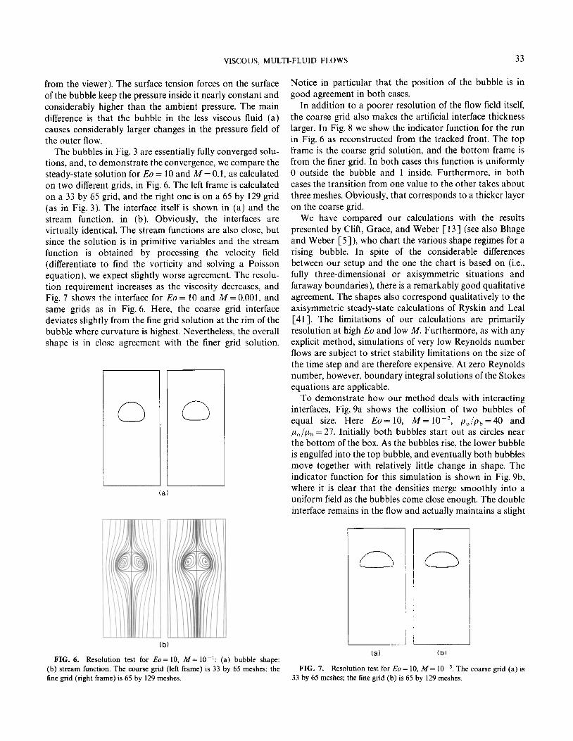
The bubbles in Fig. 3 are essentially fully converged solu- tions, and, to demonstrate the convergence, we compare the steady-state solution for Eo = 10 and M = 0.1, as calculated on two different grids, in Fig. 6. The left frame is calculated on a 33 by 65 grid, and the right one is on a 65 by 129 grid (as in Fig. 3). The interface itself is shown in (a) and the stream function, in (b). Obviously, the interfaces are virtually identical. The stream functions are also close, but since the solution is in primitive variables and the stream function is obtained by processing the velocity field (differentiate to find the vorticity and solving a Poisson equation), we expect slightly worse agreement. The resolu- tion requirement increases as the viscosity decreases, and Fig. 7 shows the interface for Eo = 10 and A4 = 0.001, and same grids as in Fig. 6. Here, the coarse grid interface deviates slightly from the line grid solution at the rim of the bubble where curvature is highest. Nevertheless, the overall shape is in close agreement with the liner grid solution.
ii 0
(a)
(b)
FIG. 6. Resolution test for Eo= 10, M= 10-l: (a) bubble shape: (b) stream function. The coarse grid (left frame) is 33 by 65 meshes; the tine grid (right frame) is 65 by 129 meshes.
Notice in particular that the position of the bubble is in good agreement in both cases.
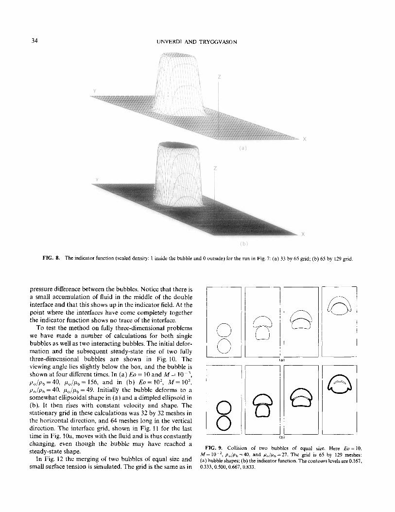
In addition to a poorer resolution of the flow field itself, the coarse grid also makes the artificial interface thickness larger. In Fig. 8 we show the indicator function for the run in Fig. 6 as reconstructed from the tracked front. The top frame is the coarse grid solution, and the bottom frame is from the liner grid. In both cases this function is uniformly 0 outside the bubble and 1 inside. Furthermore, in both cases the transition from one value to the other takes about three meshes. Obviously, that corresponds to a thicker layer on the coarse grid.
We have compared our calculations with the results presented by Clift, Grace, and Weber [ 131 (see also Bhage and Weber [S]), who chart the various shape regimes for a rising bubble. In spite of the considerable differences between our setup and the one the chart is based on (i.e., fully three-dimensional or axisymmetric situations and faraway boundaries), there is a remarkably good qualitative agreement. The shapes also correspond qualitatively to the axisymmetric steady-state calculations of Ryskin and Lea1 [41]. The limitations of our calculations are primarily resolution at high Eo and low M. Furthermore, as with any explicit method, simulations of very low Reynolds number flows are subject to strict stability limitations on the size of the time step and are therefore expensive. At zero Reynolds number, however, boundary integral solutions of the Stokes equations are applicable.
To demonstrate how our method deals with interacting interfaces, Fig. 9a shows the collision of two bubbles of equal size. Here Eo = 10, M= lo-*, pO/pb =40 and pO/pLb = 27. Initially both bubbles start out as circles near the bottom of the box. As the bubbles rise, the lower bubble is engulfed into the top bubble, and eventually both bubbles move together with relatively little change in shape. The indicator function for this simulation is shown in Fig. 9b, where it is clear that the densities merge smoothly into a uniform field as the bubbles come close enough. The double interface remains in the flow and actually maintains a slight
(a) (b)
FIG. 7. Resolution test for Eo = 10, M= lo-‘. The coarse grid (a) is 33 by 65 meshes; the tine grid (b) is 65 by 129 meshes.
34 UNVERDI AND TRYGGVASON
FIG. 8. The indica .tor function (scaled density: 1 inside the bubble and 0 outside) for the run in Fig. 7: (a) 33 by 65 grid; (b) 65 by 129 grid
(a)
(b)
pressure difference between the bubbles. Notice that there is a small accumulation of fluid in the middle of the double interface and that this shows up in the indicator field. At the point where the interfaces have come completely together the indicator function shows no trace of the interface.
To test the method on fully three-dimensional problems we have made a number of calculations for both single bubbles as well as two interacting bubbles. The initial defor- mation and the subsequent steady-state rise of two fully three-dimensional bubbles are shown in Fig. 10. The viewing angle lies slightly below the box, and the bubble is shown at four different times. In (a) Eo = 10 and M = lo-‘, pO/p,, =40, ,LL~/,u~ = 156, and in (b) Eo= lo', M= lo*, p0/pb=40, pL,/pLb = 49. Initially the bubble deforms to a somewhat ellipsoidal shape in (a) and a dimpled ellipsoid in (b). It then rises with constant velocity and shape. The stationary grid in these calculations was 32 by 32 meshes in the horizontal direction, and 64 meshes long in the vertical direction. The interface grid, shown in Fig. 11 for the last time in Fig. IOa, moves with the fluid and is thus constantly changing, even though the bubble may have reached a steady-state shape.
In Fig. 12 the merging of two bubbles of equal size and small surface tension is simulated. The grid is the same as in
0 0
0 0
(bl
FIG. 9. Collision of two bubbles of equal size. Here Eo = 10, M= 10m2, pa/p,, =40, and /.~~/fi~ =27. The grid is 65 by 129 meshes: (a) bubble shapes; (b) the indicator function. The contours levels are 0.167, 0.333,0.500,0.667,0.833.

VISCOUS, MULTI-FLUID FLOWS 35
(a) W FIG. 10. The initial deformation and rise of a three-dimensional
bubble. The bubble is shown at four different times. The simulation is on a 32 x 32 x 64 grid. The initial bubble diameter is 0.4 times the width of the computational box: (a) Eo = 10 and M = 10-3, pO/pb = 40, po/pLb = 156; (b) Eo = 10’ and M= lo*, po/pb =40, p,,/pb = 49.
Fig.lO, and Eo=50, M= 1, po/p,,==20, p,/pb=26. The bubbles are initially spherical and are put relatively close together, slightly off the centerline of the box. As the bubbles rise they deform considerably. The bottom of the top bubble folds upward and deforms the lower bubble into a “pear” shape, pointing toward the top one. The top bubble con- tinues to deform into a hemispherical shell with most of the fluid contained in the rim. The lower bubble is drawn into this shell. Initially, the back of the lower bubble deforms in a similar way as the back of the top one does, but the
FIG. 11. The interface grid for a rising bubble corresponding to the last time in Fig. 10a.
upward suction by the top bubble forms it into a somewhat cylindrical shape, eventually leaving a thin tail behind as most of the lower bubble merges with the top one. Although we have calculated the process for a longer time, the lower part of the bottom bubble is clearly underresolved in the last frame in Fig. 12, and the physical relevance of the results may therefore be doubtful beyond this stage. For low sur- face tension, as was the case here, the merging process is relatively fast compared with the rise velocity, and the bubbles move only about one bubble diameter during the coalescence process, which is in qualitative agreement with de Nevers and Wu [32], for example. For larger surface tension the coalescence process takes longer as is seen in the two-dimensional calculation in Fig. 9.
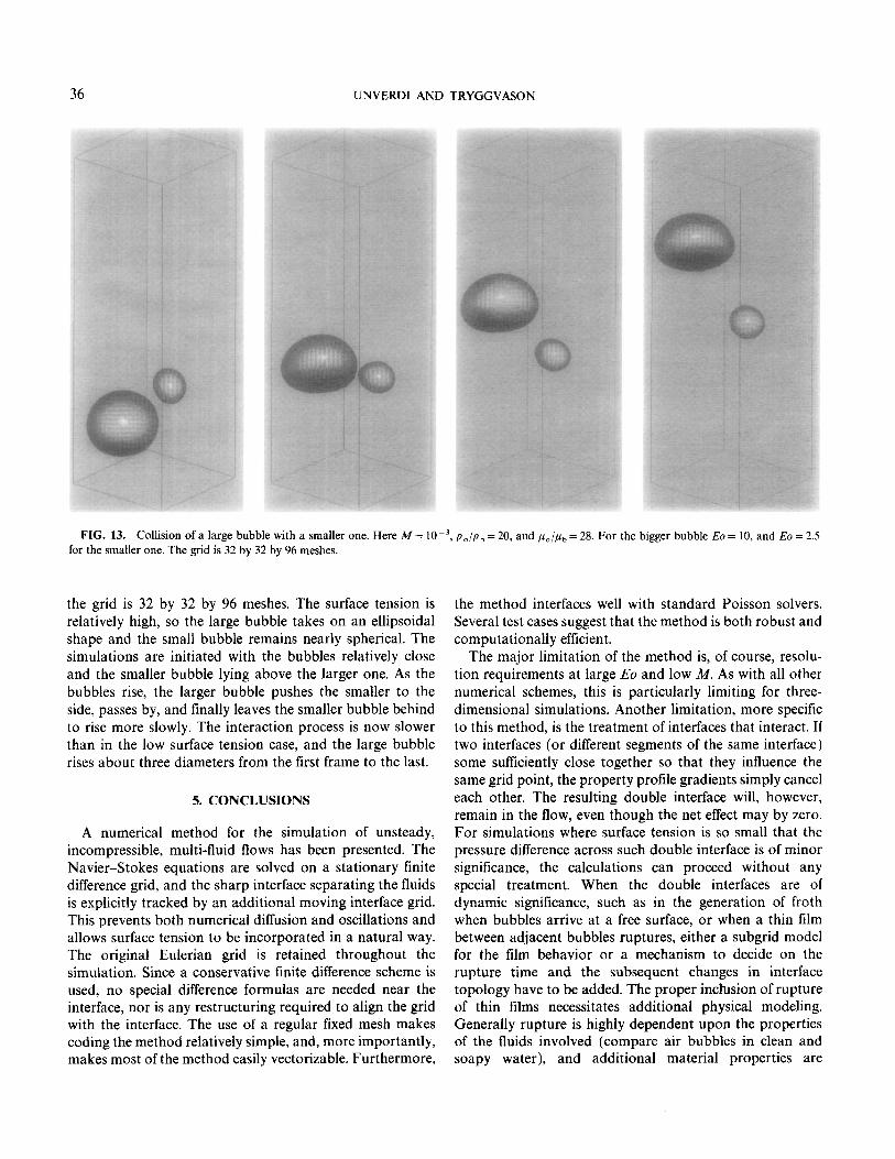
Not ali bubble interactions involve merging bubbles. In Fig. 13 the motion of a large and a small bubble is simulated. Here M = 10P3, pO/pt, = 20, pLo/pb = 28, Eo = 10, and Eo = 2.5 for the big and small bubble, respectively, and
FIG. 12. Non-axisymmetric merging of two bubbles on 32 by 32 by 64 grid. Here Eo = SO, M = I, p,/p, = 20, and p, /,ub = 26
36 UNVCWI ANIJ I KYWVASUN
FIG. 13. Collision of a large bubble with a smaller one. Here M = 10m3, p,/pb = 20, and pO/pb = 28. For the bigger bubble Eo = 10, and Eo = 2.5 for the smaller one. The grid is 32 by 32 by 96 meshes.
the grid is 32 by 32 by 96 meshes. The surface tension is relatively high, so the large bubble takes on an ellipsoidal shape and the small bubble remains nearly spherical. The simulations are initiated with the bubbles relatively close and the smaller bubble lying above the larger one. As the bubbles rise, the larger bubble pushes the smaller to the side, passes by, and finally leaves the smaller bubble behind to rise more slowly. The interaction process is now slower than in the low surface tension case, and the large bubble rises about three diameters from the first frame to the last.
5. CONCLUSIONS
A numerical method for the simulation of unsteady, incompressible, multi-fluid flows has been presented. The Navier-Stokes equations are solved on a stationary finite difference grid, and the sharp interface separating the fluids is explicitly tracked by an additional moving interface grid. This prevents both numerical diffusion and oscillations and allows surface tension to be incorporated in a natural way. The original Eulerian grid is retained throughout the simulation. Since a conservative finite difference scheme is used, no special difference formulas are needed near the interface, nor is any restructuring required to align the grid with the interface. The use of a regular fixed mesh makes coding the method relatively simple, and, more importantly, makes most of the method easily vectorizable. Furthermore,
the method interfaces well with standard Poisson solvers. Several test cases suggest that the method is both robust and computationally efficient.
The major limitation of the method is, of course, resolu- tion requirements at large Eo and low M. As with all other numerical schemes, this is particularly limiting for three- dimensional simulations. Another limitation, more specific to this method, is the treatment of interfaces that interact. If two interfaces (or different segments of the same interface) some sufftciently close together so that they influence the same grid point, the property profile gradients simply cancel each other. The resulting double interface will, however, remain in the flow, even though the net effect may by zero. For simulations where surface tension is so small that the pressure difference across such double interface is of minor significance, the calculations can proceed without any special treatment. When the double interfaces are of dynamic significance, such as in the generation of froth when bubbles arrive at a free surface, or when a thin film between adjacent bubbles ruptures, either a subgrid model for the film behavior or a mechanism to decide on the rupture time and the subsequent changes in interface topology have to be added. The proper inclusion of rupture of thin films necessitates additional physical modeling. Generally rupture is highly dependent upon the properties of the fluids involved (compare air bubbles in clean and soapy water), and additional material properties are

VISCOUS, MULTI-FLUID FLOWS 31
needed. To accomplish the actual implementation of such a rupture model a topological change algorithm (see, for example, Glimm et al. [24] ) would be necessary. The ability of the present method to deal with interacting interfaces by allowing them to form passive structures when suitable is comparable to the treatment in volume-tracking methods. (In its present form the method actually has a built-in model for thin films; it allows no rupture to take place and sets the pressure jump across the film equal to twice the jump across a single interface with the same curvature). We note that, while a volume-tracking method can also account for the interaction of two interfaces, modeling of thin films and rupture is completely inaccessible to volume-tracking, since a double interface will always disappear whether it is physical or not.
Although our method has been tested extensively on two- dimensional problems, the major purpose of developing it was to simulate fully three dimensional situations. The test cases presented here suggest that larger simulations involving several bubbles are entirely feasible, although such simulations will, naturally, always be limited to some- what modest-sized systems. Our experience suggests that, for high viscosity and high surface tension, a meaningful resolution of a single bubble can be achieved on a grid as small as 16’ (our three-dimensional bubbles had a diameter of about 16 meshes). Larger simulations, for example, on a 643 or a 1283 grid, could include several bubbles.
ACKNOWLEDGMENTS
We wish to acknowledge the help of C. Churchill at the University of Michigan Visualization Laboratory with the graphics, and P. Wesseling at the University of Delft who sent us his multigrid code (MGD). This work was supported by NSF Grant No. MSM87-07646. The calculations were done on the computers at the San Diego Supercomputer Center which is sponsored by the NSF.
REFERENCES
I. A. Acrivos, “The Deformation and Break-up of Single Drops in Shear Fields,” in Physicochemical Hydrodynamics, Inlerfacial Phenomena, edited by M. G. Velarde (Plenum, New York, 1987) p. 1.
2. C. R. Anderson, J. Comput. Phys. 61,417 (1985). 3. A. A. Amsden and F. H. Harlow, J. Comput. Phys. 6, 322 (1970).
4. G. R. Baker and D. W. Moore, Phys. Fluids A 1, 1451 (1989).
5. D. Bhaga and M. E. Weber, J. Fluid Mech. 105,61 (1981).
6. S. H. Brecht and J. R. Ferrante, Phys. Fluids A 1, 1166 (1989).
7. J. P. Boris, Annu. Rev. Fluid Mech. 21, 345 (1989). 8. I.-L. Chern, J. Glimm, 0. McBryan, B. Plohr, and S. Yaniv, J. Comput.
Phys. 62, 83 (1986).
9. B. K. Chi and L. G. Leal, J. Fluid Mech. 201, 123 (1989).
IO. A. J. Chorin, J. Compuf. Phys. 35, 1 (1980).
Il. J. P. Christiansen, J. Comput. Phys. 13, 363 (1973).
12.
13.
14.
15.
16.
17.
18.
19.
20.
21.
22.
23.
24.
25.
26.
27.
28.
29.
30.
31.
32.
33.
34.
35.
36.
37.
38.
39.
40.
41.
42.
43.
44.
45.
46. A-l
H. A. Stone and L. G. Leal, J. Fluid Mech. 198, 399 (1989).
H. A. Stone and L. G. Leal, J. Fluid Mech. 220, 161 (1990).
P. H. Todd and R. J. Y. McLeod, Cornput. Aided Design 18, 33 (1986). 7,.
48.
49.
G. Tryggvason, J. Comput. Phys. 75, 253 (1988).
G. Tryggvason and S. 0. Unverdi, Phys. Fluids A 2, No. 5, 656 (1990).
P. Wesseling, “A Robust and Efficient Multigrid Method,” in Mull&id Methods, edited by W. Hackbusch and U. Trottenberg (Proceedings, KolnPorz, 1981) Lect. Notes in Math., Vol. 960 (Springer-Verlag, Berlin, 1982), p. 614.
50. G. K. Youngren and A. Acrivos, J. Fluid Mech. 76, 433 (1976). 51. S. G. Yiantsios and B. G. Higgins, Phys. F/uids A 1, 1484 (1989).
S. W. Churchill, “Viscous Flows. The Practical Use of Theory” (Butterworths, London, 1988).
R. Clift, J. R. Grace, and M. E. Weber, “Bubbles, Drops, and Particles” (Academic Press, New York/London, 1978).
D. S. Dandy and L. G. Leal, J. Fluid Mech. 208, 161 (1989).
B. J. Daly, Phys. Fluids 10, 297 (1967). B. J. Daly, J. Comput. Phys. 4, 97 (1969).
P. Daripa, J. Glimm, B. Lindquist, M. Maesumi, and 0. McBrian, “On the Simulation of Heterogeneous Petroleum Reservoirs,” in Numerical Simulation in Oil Recovery, edited by M. Wheeler (Springer Verlag, New York, 1988).
J. M. Floryan and H. Rasmussen, Appl. Mech. Rev. 42, 323 (1989).
L. J. Fauci and C. S. Peskin, J. Comput. Phys. 77, 80 (1988).
A. L. Fogelson and C. S. Peskin, J. Comput. Phys. 79, 50 (1988).
M. J. Fritts and J. P. Boris, J. Compuf. Phys. 31, 173 (1979).
D. E. Fyfe, E. S. Oran, and M. J. Fritts, J. Comput. Phys. 76, 349 (1988).
J. Glimm, 0. McBryan, R. Menikoff, and D. H. Sharp, SIAM J. Sci. Stat. Comput. 7, 230 (1987).
J. Glimm, J. Grove, B. Lindquist, 0. McBryan, and G. Tryggvason, SIAM J. Sci. Stat. Comput. 9,61 (1988).
F. H. Harlow and J. E. Welch, Phys. Fluids 8, 2182 (1965).
C. W. Hirt and B. D. Nichols, J. Comput. Phys. 39, 201 (1981).
J. M. Hyman, Physica D 12, 396 (1984). C. J. Koh and L. G. Leal, Phys. Fluids A 1, 1309 ( 1989). M. J. Martinez and K. S. Udell, J. Fluid Mech. 210, 565 (1990).
J. C. S. Meng and J. A. L. Thomson, J. Fluid Mech. 84,433 (1978).
G. Moretti, Annu. Rev. Fluid Mech. 19, 313 (1987).
N. de Nevers and J.-L. Wu, AIChE J. 17, 182 (1971).
W. F. Noh and P. Woodward, Lecture Notes in Physics, Vol. 59 (Springer-Verlag, New York/Berlin, 1976) p. 330.
E. S. Oran and J. P. Boris, Numerical Simulafions of Reuclive Fiow (Elsevier, Amsterdam/New York, 1987).
C. S. Peskin, J. Comput. Phys. 25, 220 (1977).
C. Pozrikidis, J. Fluid Mech. 210, 1 (1990).
J. M. Rallison, J. Fluid Mech. 109, 465 (1981).
J. M. Rallison, Annu. Rev. Fluid Mech. 16, 45 (1984). R. D. Richtmyer and K. W. Morton, Bfference Methods for Initial- Value Problems (Interscience, New York, 1967).
G. Ryskin and L. G. Leal, J. Fluid Mech. 148, 1 (1984). G. Ryskin and L. G. Leal, J. Fluid Mech. 148, 19 (1984). G. Ryskin and L. G. Leal, J. Fluid Mech. 148, 37 (1984).
H. A. Stone, B. J. Bentley, and L. G. Leal, J. Fluid Mech. 173, 131 (1986).