A FRAMEWORK FOR THE ADAPTIVE FINITE ELEMENT …bangerth/publications/2007-si… · ·...

Copyright © by SIAM. Unauthorized reproduction of this article is prohibited.

SIAM J. SCI. COMPUT. c© 2008 Society for Industrial and Applied MathematicsVol. 30, No. 6, pp. 2965–2989

A FRAMEWORK FOR THE ADAPTIVE FINITE ELEMENTSOLUTION OF LARGE-SCALE INVERSE PROBLEMS∗

WOLFGANG BANGERTH†

Abstract. Since problems involving the estimation of distributed coefficients in partial differ-ential equations are numerically very challenging, efficient methods are indispensable. In this paper,we will introduce a framework for the efficient solution of such problems. This comprises the useof adaptive finite element schemes, solvers for the large linear systems arising from discretization,and methods to treat additional information in the form of inequality constraints on the parameterto be recovered. The methods to be developed will be based on an all-at-once approach, in whichthe inverse problem is solved through a Lagrangian formulation. The main feature of the paper isthe use of a continuous (function space) setting to formulate algorithms, in order to allow for dis-cretizations that are adaptively refined as nonlinear iterations proceed. This entails that steps suchas the description of a Newton step or a line search are first formulated on continuous functions andonly then evaluated for discrete functions. On the other hand, this approach avoids the dependenceof finite dimensional norms on the mesh size, making individual steps of the algorithm comparableeven if they used differently refined meshes. Numerical examples will demonstrate the applicabil-ity and efficiency of the method for problems with several million unknowns and more than 10,000parameters.

Key words. adaptive finite elements, inverse problems, Newton method on function spaces

AMS subject classifications. 65N21, 65K10, 35R30, 49M15, 65N50

DOI. 10.1137/070690560

1. Introduction. Parameter estimation methods are important tools in caseswhere quantities we would like to know, such as material parameters, cannot bemeasured directly, but where only measurements of related quantities are available.In such cases one attempts to find a set of parameters for which the predictions ofa mathematical model, the equation of state, best match what has actually beenobserved. Parameter estimation is therefore a problem that can be described asan optimization problem: minimize, by variation of the unknown parameter, themisfit between prediction and actual observation, subject to the constraint that theprediction satisfies the state equation.

If the state equation is a differential equation, such parameter estimation problemsare commonly referred to as inverse problems. These problems have a vast number ofapplications—for example, identification of the underground structure (e.g., the elas-tic properties, density, electric or magnetic permeabilities of the earth) from measure-ments at the surface, or of the groundwater permeability of a soil from measurementsof the hydraulic head fall in this class. Likewise, many biomedical imaging modalities,such as computer tomography, electrical impedance tomography, or several optical to-mography modalities, can be cast as inverse problems.

The case we are interested in here is recovering a distributed, i.e., spatially variable,coefficient. Oftentimes, such problems are found when trying to identify inhomoge-nous material properties as in the examples mentioned above. In particular, we will

∗Received by the editors May 4, 2007; accepted for publication (in revised form) March 3, 2008;published electronically October 13, 2008. Part of this work was funded by the National ScienceFoundation under grant DMS-0604778.

http://www.siam.org/journals/sisc/30-6/69056.html†Department of Mathematics, Texas A&M University, College Station, TX 77843-3368

([email protected]).

2965


2966 WOLFGANG BANGERTH

consider cases where we make many experiments to identify the parameters. Here,by an experiment we mean subjecting the physical system to a certain forcing andmeasuring its response. For example, in computer tomography, a single experimentwould be characterized by irradiating a body from a given angle and measuring thetransmitted part of the radiation; the multiple experiment situation is characterizedby using data from various incidence angles and trying to find a set of parametersthat matches all the measurements at the same time (joint inversion). Likewise, ingeophysics, a single experiment would be placing a seismic source somewhere andmeasuring reflection data at various receiver positions; the multiple experiment caseis taking into account data from more than one source position. We may also includeentirely different kinds of data, e.g., use both magneto-telluric and gravimetry datafor a joint, multiphysics inversion scenario.

This paper is devoted to the development of efficient techniques for the solution ofsuch inverse problems where the state equation is a partial differential equation (PDE)and the parameters to be determined are one or several distributed functions. It iswell known that the numerical solution of PDE constrained inverse or optimizationproblems is significantly more challenging than that of a PDE alone (see, e.g., [15]),since the optimization procedure is usually iterative and in each iteration may needthe numerical solution of a large number of partial differential equations. In someapplications, several tens or hundreds of thousand solutions of linearized PDEs arerequired to solve the inverse problem, and each PDE may be discretized by up toseveral hundred thousand unknowns.

Although it is obvious that efficiency of solution is a major concern for this classof problems, efficient methods such as adaptive finite element techniques have not yetfound widespread application to inverse problems and are only slowly adopted in thesolution of PDE constrained optimization [10, 11, 13, 21, 22, 30, 31, 32, 35, 39, 46,50, 51]. Rather, in most cases, the continuous inverse problem is first discretized ona predetermined mesh, and the resulting nonlinear problem is then solved using well-understood finite dimensional methods such as Newton’s method or a variant of it.On the other hand, discretizations cannot be changed by adapting the mesh betweennonlinear iterations, and the potential to significantly reduce the numerical cost bytaking into account the spatial structure of solutions is lost. This is because a changein the discretization changes the size of finite dimensional problems, rendering finitedimensional convergence criteria such as norms meaningless.

The goal for this paper is therefore to devise a framework for adaptive finiteelement techniques. By using such adapted meshes, we can not only significantlyreduce the numerical effort needed to solve inverse parameter estimation problems,but the ability to choose a discretization mesh coarse where we lack information orwhere a fine mesh is not required also makes the inverse problem better posed. Toachieve this goal, the main novel ingredients will be the following:

• formulation of all algorithms in function spaces, i.e., before rather than afterdiscretization, since this gives us more flexibility in discretizing as iterationsproceed and resolves all scaling issues related to differing mesh sizes;

• the use of adaptive finite element techniques with mesh refinement based ona posteriori error estimates;

• the use of different meshes for the discretization of different quantities, forexample, of state variables and of parameters, to reflect their respective prop-erties;

• the use of Newton-type methods for the outer (nonlinear) iteration and ofefficient linear solvers for the Newton steps;


ADAPTIVE FEM SOLUTION OF INVERSE PROBLEMS 2967

• the use of approaches that allow for the parallelization of work, yielding sub-problems that are equivalent to only state and adjoint problems; and

• the inclusion of pointwise bounds on the parameters into the solution process.Except for the derivation of error estimates, which we defer to future work (see also[4]), we will discuss all these building blocks and will show that these techniques allowus to solve problems of the size outlined above.

We envision that the techniques to be presented are used for relatively complexproblems. Thus, we will state them in the setting of a generic inverse problem. Inorder to explain their concrete structure, we will define a model problem involving thePoisson equation and apply the framework to it. Numerical examples at the end ofthe paper will show this model problem as well as application of the framework to asignificantly more complex case in optical tomography. Applications of the frameworkto other problems in acoustic scattering can be found in [4], and further work in opticaltomography in biomedical imaging is also presented in [7, 40, 41].

Solving large-scale, multiple-experiment inverse problems requires algorithms onseveral levels, all of which have to be tailored to high efficiency. In this article, wewill review the building blocks of a framework for this:

• formulation as a Lagrangian optimization problem with PDE constraints (sec-tion 2); a model problem is given in section 3;

• outer nonlinear solution by a Gauss–Newton method posed in function spaces(section 4);

• discretization of each Newton step by finite elements on independent meshes(section 5);

• Schur complement solvers for the resulting linear systems (section 6);• methods to incorporate bound constraints on the parameters (section 7).

Section 8 is devoted to numerical examples, followed by conclusions in the final section.

2. General formulation and notation. Let us begin by introducing some ab-stract notation, which we will use for the derivation of the entire scheme. This, aboveall, concerns the set of parameters, state equations, measurements, regularization,and the introduction of an abstract Lagrangian.

We note that some of the formulas below will become cumbersome to read becauseof the number of indices. To understand their meaning, it is often helpful to imaginewe had only a single experiment (for example, only one incidence angle in tomography,or only one source position in seismic imaging). In this case, one may drop the indexi on first reading, as well as all summations over i. In addition, the formulas of thissection will be made concrete by introducing a model problem in section 3.

State equations. Let the general setting of the problems we consider be as fol-lows: assume that we subject a physical system to i = 1, . . . , N different externalstimuli and that we intend to learn about the system’s material parameters by mea-suring how the system reacts. For the current purposes, we assume that the system’sstates can be described by (independent) partial differential equations posed on adomain Ω ⊂ R

d:

Ai[q] ui = f i in Ω,(2.1)

Bi[q] ui = hi on ΓiN ⊂ ∂Ω,(2.2)

ui = gi on ΓiD = ∂Ω\Γi

N ,(2.3)

where Ai[q] are partial differential operators all of which depend on a common set of apriori unknown distributed (i.e., spatially variable) coefficients q = q(x) ∈ Q, x ∈ Ω,



and Bi[q] are boundary operators that may also depend on the coefficients. f i, hi,and gi are the known external forcing terms that are independent of the coefficientsq. The functions ui are the solutions of the partial differential equations, i.e., thephysical outcomes (“states”) of our N experiments. These scalar or vector-valuedsolutions are assumed to be from spaces V i

g = {ϕ ∈ V i : ϕ|ΓiD

= gi}. We assume that

solutions ui, uj of different equations are independent except for their dependence onthe common set of parameters q. We also assume that the solutions to each of thedifferential equations is unique for every given set of parameters q in a subset Qad ⊂ Qof physically meaningful values, for example, Qad = {q ∈ L∞(Ω) : q0 ≤ q(x) ≤ q1}.

Typical cases we have in mind would be a Laplace-type equation when we are con-sidering electrical impedance tomography or gravimetry inversion, Helmholtz or waveequations for inverting seismic or magneto-telluric data, or diffusion-reaction equa-tions for optical tomography applications. The set of parameters q would, in thesecases, be electrical conductivities, densities, elasticity coefficients, or optical proper-ties. The operators Ai may be the same if we repeat the same kind of experimentmultiple times with different forcings, but they will be different if we use differentphysical effects (for example gravimetry and seismic data) to identify q.

This formulation may easily be extended also to the case of time-dependent prob-lems. Likewise, the case that the parameters are a finite number of scalar valuesinstead of distributed functions is a simple special case, omitted here for brevity.

For treatment in a Lagrangian setting in function spaces as well as for discretiza-tion by finite elements, it is necessary to formulate the state equations (2.1)–(2.3) ina variational form. For this we assume that the solutions ui ∈ V i

g are solutions of thefollowing variational equalities:

(2.4) Ai(q;ui)(ϕi) = 0 ∀ϕi ∈ V i0 ,

where V i0 = {ϕi ∈ V i : ϕi|Γi

D= 0}. The semilinear form Ai : Q× V i

g × V i0 → R may

be nonlinear in its first set of arguments but is linear in the test function and includesthe actions of domain and boundary operators Ai and Bi as well as of inhomogeneousforcing terms. We will later have to assume that the Ai are differentiable.

As an example, we will introduce a model problem for the Poisson equation. Inthat case, Ai[q]ui = −∇ · (q∇ui), Bi[q]ui = q∂nu

i, and

A(q;ui)(ϕi) = (q∇ui,∇ϕi)Ω − (f, ϕi)Ω − (h, ϕi)ΓN.

Measurements. To determine the unknown quantities q, we measure how thephysical system reacts to the external forcing, i.e., we measure (parts of) the statesui or derived quantities. For example, we might have measurements of voltages,optical fluxes or stresses at certain points, averages on subdomains, or gradients.Let us denote the space of measurements of the ith state variable by Zi, and letM i : V i

g → Zi be the measurement operator, i.e., the operator that extracts from

physical state ui that information that we measure.If we knew the parameters q, we could use the state equation (2.4) to predict the

state the system would be in, and M iui would then be the predicted measurements.On the other hand, we do not know q, but we have actual measurements that wedenote by zi ∈ Zi. Reconstruction of the coefficients q will be accomplished byfinding that coefficient, for which the predicted measurements M iui match the actualmeasurements zi best. We will measure this comparison using a convex, differentiablefunctional m : Zi → R. In many cases, m will simply be an L2 norm on Zi, but more



general functionals are allowed, for example, to suppress the effects of non-Gaussiannoise [54].

Examples of common measurement situations are as follows:• L2 measurements of values. If measurements on a set Σ ⊂ Ω are available,

then M i is the embedding operator from V ig into Zi = L2(Σ), and we will

try to find q by minimizing

mi(M iui − zi) =1

2‖ui − zi‖2

L2(Σ).

In many nondestructive testing or tomography applications, one has Σ ⊂ ∂Ωbecause measurements in the interior are not possible. The case of distributedmeasurements occurs in situations where a measuring device can be movedaround to every point of Σ, for example, a laser scanning a membrane, or acamera imaging a body.

• Point measurements. If we have S measurements of u(x) at positions xs ∈Ω, s = 1, . . . , S, then Zi = R

S , and (M iui)s = u(xs). If we take again aquadratic norm on Zi, then, for example,

mi(M iui − zi) =1

2

S∑s=1

|ui(xs) − zis|2

is a possible choice. The case of point measurements is frequent in applica-tions where a small number of stationary measurement devices is used, forexample, seismometers in seismic data assimilation.

Other choices are possible and are usually dictated by the type of available measure-ments. We will in general assume that the operators M i are linear, but there areapplications where this is not the case. For example, in some applications only sta-tistical correlations of ui are known, or a power spectrum. Extending the algorithmsbelow to nonlinear M i is straightforward, but we omit this for brevity.

Regularization. Since inverse problems are often ill-posed, regularization isneeded to suppress unwanted features in solutions q. In this work, we include itby using a Tikhonov regularization term involving a convex differentiable regular-ization functional r : Q → R

+; see, for example, [27, 44]. Most frequently r(q) =12‖∇t(q− q)‖2

L2(Ω) with an a priori guess q and some t ≥ 0. Other popular choices are

smoothed versions of bounded variation seminorms [24, 26, 29]. As above, the typeof regularization is usually dictated by the application and insight into physical andunphysical features of solutions.

Characterization of solutions. The goal of the inverse problem is to find thatset of physical parameters q ∈ Qad for which the predictions M iui match the actualobservations zi best. We formulate this as the following constrained minimizationproblem over ui ∈ V i

g , q ∈ Qad:

minimize J({ui}, q) =

N∑i=1

σimi(M iui − zi) + βr(q)(2.5)

such that Ai(q;ui)(ϕi) = 0 ∀ϕi ∈ V i0 , 1 ≤ i ≤ N.

Here, σi > 0 are factors weighting the relative importance of individual measurements,and β > 0 is a regularization parameter. As the choice of these constants is a topicof its own, we assume their values as given within the scope of this work.



To characterize solutions to (2.5), let us subsume the individual solutions ui toa vector u, and likewise Vg = {V i

g },V0 = {V i0 }. Furthermore, we introduce a set of

Lagrange multipliers λ ∈ V0 and denote the joint set of variables by x = {u,λ, q} ∈Xg = Vg × V0 ×Q.

Under appropriate conditions (see, e.g., [9]), solutions of problem (2.5) are sta-tionary points of the following Lagrangian L : Xg → R, which couples the functionalJ : Vg ×Q → R

+ defined above to the state equation constraints through Lagrangemultipliers λi ∈ V i

0 :

(2.6) L(x) = J(u, q) +

N∑i=1

Ai(q;ui)(λi).

The optimality conditions then read in abstract form

(2.7) Lx(x)(y) = 0 ∀y ∈ X0,

where the semilinear form Lx : Xg × X0 → R is the derivative of the Lagrangian L,and X0 = V0 × V0 × Q. Indicating derivatives of functionals with respect to theirarguments by subscripts, we can expand (2.7) to yield the following set of nonlinearequations:

Lλi(x;ϕi) ≡ Ai(q;ui)(ϕi) = 0 ∀ϕi ∈ V i0 ,(2.8)

Lui(x;ψi) ≡ σimiu(M iui − zi)(ψi) + Ai

u(q;ui)(ψi, λi) = 0 ∀ψi ∈ V i0 ,(2.9)

Lq(x;χ) ≡ βrq(q)(χ) +

N∑i=1

Aiq(q;u

i)(χ, λi) = 0 ∀χ ∈ ∂Q.(2.10)

The first set of equations denotes the state equations for i = 1, . . . , N and the secondthe adjoint equations defining the Lagrange multipliers λi; the third is the controlequation holding for all functions from the tangent space ∂Q to Q at the solution q.

3. A model problem. As a simple model problem which we will use to givethe abstract results of this work a more concrete form, we will consider the followingsituation. Assume we intend to identify the coefficient q in the (single) elliptic PDE

−∇ · (q∇u) = f in Ω, u = g on ∂Ω,(3.1)

and that measurements are the values of the solution u everywhere in Ω, i.e., wechoose m(Mu−z) = 1

2‖u−z‖2L2(Ω). This situation can be considered as a mathemat-

ical description of a membrane with variable stiffness q(x). We try to identify thiscoefficient by subjecting the membrane to a known force f and clamping it at theboundary with boundary values g. This results in displacements of which we obtainmeasurements z everywhere.

For this situation, Vg = {u ∈ H1 : u|∂Ω = g}, Q ⊂ L∞. Choosing σ = 1, theLagrange functional has the form

L(x) = 12‖u− z‖2

L2(Ω) + βr(q) + (q∇u,∇λ) − (f, λ).

With this, the optimality conditions (2.8)–(2.10) read in weak form

(q∇u,∇ϕ) = (f, ϕ),(3.2)

(q∇ψ,∇λ) = −(u− z, ψ),(3.3)

βrq(q;χ) = −(χ∇u,∇λ)(3.4)

and have to hold for all test functions {ϕ,ψ, χ} ∈ H10 ×H1

0 ×Q. Note that the firstof these is the state equation, while the second is the adjoint equation.



4. Nonlinear solvers. The stationarity conditions (2.7) form a set of nonlinearpartial differential equations that has to be solved iteratively, for example, usingNewton’s method, or a variant thereof. In this section, we formulate the Gauss–Newton method in function spaces. The discretization of each step by adaptive finiteelements will then be presented in the next section, followed by a discussion of solversfor the resulting linear systems.

Since there is no need to compute the initial nonlinear steps on a very fine gridwhen we are still far away from the solution, we will want to use successively finermeshes as we approach the solution. To make quantities computed on different meshescomparable, all of the following algorithms will be formulated in a continuous settingand only then will be discretized. This also answers once and for all questions aboutthe correct scaling of weighting matrices in misfit and regularization functionals, asdiscussed, for example, in [2], even if we choose locally refined grids, as they willappear naturally upon discretization.

In this section, we indicate a Gauss–Newton procedure, i.e., determination ofsearch direction and step length, in infinite dimensional spaces, and in the next sectionwe discuss its discretization by a finite element scheme. At least for finite-dimensionalproblems, there is a vast number of alternatives to the Gauss–Newton method; see,for example, [1, 23, 34, 38, 47, 48, 53]. However, we believe that the Gauss–Newtonmethod is particularly suited since it allows for scalable algorithms even with largenumbers of experiments, and large numbers of degrees of freedom both in the dis-cretization of the state equations as well as of the parameter. Comparing this methodto a pure Newton method, it allows for the use of more efficient linear solvers for thediscretized problems; see section 6. In addition, the Gauss–Newton method has beenshown to have better stability properties for parameter estimation problems than theNewton method; see [18, 19]. This and similar methods have also been analyzedtheoretically; see, for example, [36, 37, 55] and the references cited therein.

Strictly speaking, the algorithms we propose below may converge to a local max-imum or saddle point. This does not appear to happen for the problems shown insection 8, possibly a result of the kind of state equations we consider there. Moresophisticated algorithms may add steps to safeguard against this possibility.

Search directions. Given a current approximation xk = {uk,λk, qk} ∈ X afterk iterations, the first task of any iterative nonlinear solver method is to compute asearch direction δxk = {δuk, δλk, δqk} ∈ Xδg, in which we seek the next iterate xk+1.The Dirichlet boundary values δg of this update are chosen as δui

k|ΓD= gi − ui

k|ΓD,

δλik|ΓD

= 0, bringing us to the exact boundary values if we take a full step.The Gauss–Newton method determines search directions {δuk, δqk} by minimiz-

ing the following quadratic approximation to J(·, ·) with linearized constraints:

minδuk,δqk

J(uk, qk) + Ju(uk, qk)(δuk) + Jq(uk, qk)(δqk)

+1

2Juu(uk, qk)(δuk, δuk) +

1

2Jqq(uk, qk)(δqk, δqk)

such that Ai(qk;uik)(ϕ

i) + Aiu(qk;u

ik)(δu

ik, ϕ

i) + Aiq(qk;u

ik)(δqk, ϕ

i) = 0,

(4.1)

where the linearized constraints are understood to hold for 1 ≤ i ≤ N and for all testfunctions ϕi ∈ V i

0 . The solution of this problem provides us with updates δuk, δqkfor the state variables and the parameters. The updates for the Lagrange multiplierδλk are not determined by the Gauss–Newton step at first. However, we can getupdates δλk for the original problem by using λk + δλk as Lagrange multiplier for



the constraint of the Gauss–Newton step (4.1). Bringing the terms with λk to theright-hand side, the updates are then characterized by the system of linear equations

σimiuu(M iui

k − zi)(δuik, ϕ

i) + Aiu(qk;u

ik)(ϕ

i, δλik) = −Lui(xk)(ϕ

i),

Aiu(qk;u

ik)(δu

ik, ψ

i) + Aiq(qk;u

ik)(δq

ik, ψ

i) = −Lλi(xk)(ψi),∑

i

Aiq(qk;u

ik)(χ, δλ

ik) + βrqq(qk)(δqk, χ) = −Lq(xk)(χ)

(4.2)

for all test functions {ϕi, ψi, χ}. The right-hand side of these equations is the negativegradient of the original Lagrangian, given already in the optimality condition (2.8)–(2.10).

Note that the equations determining the updates for the ith experiment decouplefrom all other experiments, except for the last equation. This will allow us to solvethem mostly separated, and in particular it allows for simple parallelization by placingthe description of different experiments onto different machines. Furthermore, the firstand second equations can be solved sequentially.

To illustrate these equations, we state their form for the model problem of sec-tion 3. In this case, the above system reads

(δuk, ϕ) + (∇δλk, qk∇ϕ) = − Lu(xk)(ϕ),

(∇ψ, qk∇δuk) + (∇ψ, δqk∇uk) = − Lλ(xk)(ψ),

(∇δλk, χ∇uk) +βrqq(qk)(δqk, χ) = − Lq(xk)(χ)

with the right-hand sides being the gradient of the Lagrangian given in section 3.In general, this continuous Gauss–Newton direction will not be computable an-

alytically. We will therefore approximate it by a finite element function δxk,h, asdiscussed in the next section.

As a final remark, let us note that the pure Newton method would read

(4.3) Lxx(xk)(δxk, y) = −Lx(xk)(y) ∀y ∈ X0,

where Lxx(xk)(·, ·) denotes the bilinear form of second variational derivatives of theLagrangian L at position xk. The Gauss–Newton method can alternatively be ob-tained from this by simply dropping all terms that are proportional to the Lagrangemultiplier λk. This is based on considering (2.9) or (3.3): λi is proportional toM iui − zi and thus will be small if M iui − zi is small, assuming stability of the(linear) adjoint operator.

Step lengths. Once we have a search direction δxk, we have to decide how farto go in this direction starting at xk to obtain the next iterate xk+1 = xk + αkδxk.In constrained optimization, a merit function including the minimization functionalJ(·) as well as the violation of the constraints is usually used for this [52].

One particular problem here is the infinite dimensional nature of the state equa-tion constraint, with the residual of the state equation being in the dual space, V ′

0 , ofV0 (which, for the model problem, is H−1). Consequently, it is unclear which normto use and whether we need to weight a violation of the state equation in differentparts of the domain differently. Furthermore, the relative weighting of constraint andobjective function is not obvious.

To avoid these problems, we propose to use the norm of the residual of the opti-mality condition (2.7) on the dual space of X0 as merit function:

p(α) =1

2‖Lx(xk + αδxk)(·)‖2

X ′0≡ 1

2supy∈X0

[Lx(xk + αδxk)(y)]2

‖y‖2X0

.



We will show in the next section that we can give a simple-to-compute lower boundfor p(·) using the discretization we already employ for the computation of δxk.

The following lemma shows that this merit function is actually useful.Lemma 4.1. The merit function p(α) is valid, i.e., Newton directions are direc-

tions of descent, p′(0) < 0. Furthermore, if xk = x is a solution of the parameterestimation problem, then p(0) = 0. Finally, in the vicinity of the solution, full stepsare taken, i.e., α = 1 minimizes p as xk → x.

Proof. We prove the lemma for the special case of only one experiment (N = 1)and that X = H1

0 ×H10 × L2, i.e., the situation of the model example. However, it is

obvious how to extend the proof to the general case. In this simplified situation, bythe Riesz theorem there is a representation gu(xk +αδxk) = Lu(xk +αδxk)(·) ∈ H−1,gλ(xk+αδxk) = Lλ(xk+αδxk)(·) ∈ H−1, and gq(xk+αδxk) = Lq(xk+αδxk)(·) ∈ L2.The dual norm of Lx can then be written as

‖Lx‖2X ′

0=

⟨gu, (−Δ)−1gu

⟩+⟨gλ, (−Δ)−1gλ

⟩+ (gq, gq),

where (−Δ)−1 : H−1 → H10 and where 〈·, ·〉 indicates the duality pairing between

H−1 and H10 . Then,

p′(0) =⟨guu(δuk), (−Δ)−1gu

⟩+⟨gλλ(δλk), (−Δ)−1gλ

⟩+ (gqq(δqk), gq),

where gux(δxk) is the derivative of gu in direction δxk, i.e., the functional of secondderivatives of L. However, by definition of the Newton direction, (4.3), this is equalto the negative gradient, i.e.,

p′(0) = −‖Lx(xk)‖2X ′

0= −2p(0) < 0.

Thus, Newton directions are directions of descent for this merit function.The second part of the lemma is obvious by noting the optimality condition (2.7).

The last part can be shown by noting that near the solution, the Lagrangian (andthus the function p(α)) is well approximated by a quadratic function if the variousfunctionals involved in the Lagrangian are sufficiently smooth. As xk → x, Newtondirections satisfy δxk → x − xk and minα p(α) → 0. On the other hand, it is easyto show that quadratic functions with p′(0) = −2p(0) and minα p(α) = 0 have theirminimum at α = 1. A complete proof would require the more involved step of showinguniformity estimates of the Hessian Lxx in a ball around the solution. This must beshown for each individual application; since this paper is concerned with a generalframework, rather than a particular application, we omit this step here.

5. Discretization. The goal for the preceding section was to provide the func-tion space tools to find a solution x of the inverse problem. To actually computefinite-dimensional approximations to x, we have to discretize both the state and ad-joint variables, as well as the parameters. In this section, we introduce finite elementschemes to do so. The main point is to be able to change meshes between Gauss–Newton iterations. This has at least three advantages over an a priori choice of amesh: (i) it makes the initial iterations significantly cheaper when we are still faraway from the solution; (ii) coarser meshes act as an additional regularization, mak-ing the problem better posed; and (iii) it allows us to adapt the resolution of the meshto the characteristics of the solution.

In each iteration, we define finite element spaces Xh ⊂ X over triangulations inthe usual way. In particular, let T

ik be the mesh on which to discretize state and



adjoint variables uik, λ

ik of the ith experiment in the kth Gauss–Newton iteration.

Independently, a mesh Tqk will be used to discretize the parameters q on step k.

This reflects that the regions of missing regularity of parameters and state variablesneed not necessarily coincide. We may also use different discretization spaces forparameters and state/adjoint variables, for example, spaces of discontinuous functionsfor quantities like density or elasticity coefficients. On the other hand, we use the samemesh T

ik for state and adjoint variables; maybe the most important reason for this

is that not doing so would create significantly more work in assembling matrices andvectors for the operations discussed below; the matrices Ai would also not necessarilybe square any more and may not be invertible.

For these grids and the finite element spaces defined on them, we assume thefollowing requirements:

• Nesting. The mesh Tik must be obtainable from T

ik−1 by hierarchic coarsening

and refinement. This greatly simplifies operations like evaluation of the right-hand side of the Newton direction equation, Lx(xk)(yk+1) for all discrete testfunctions yk+1, but also the update operation xk+1 = xk + αkδxk,h.

• State versus parameter meshes. Each of the “state meshes” Tik can be ob-

tained by hierarchical refinement from the “parameter mesh” Tqk.

Although obvious, the choice of entirely independent grids for state and parametermeshes apparently has not been used in the literature, to the author’s best knowledge.On the other hand, this technique offers the prospect of greatly reducing the amountof numerical work. We will see that with the requirements on the meshes above, theadditional work associated with using different meshes is in fact small.

Choosing different “state” and “parameter meshes” is also beneficial for problemswhere the parameters do not require high resolution, or require it only in certain areasof the domain, while the state equation does. A typical problem is high-frequencypotential scattering, where the coefficient might be a function that is constant inlarge parts of the domain, while the high-frequency oscillations of state and adjointvariables require a fine grid everywhere.

In the next few paragraphs, we briefly describe the process of discretizing theequations for the search directions and the choice of the step length. We then give abrief note on the criteria for generating the meshes on which we discretize.

Search directions. By choosing a finite dimensional subspace Xh = Vh × Vh ×Qh ⊂ X and a basis of this space, we obtain a discrete counterpart for (4.2) describingthe Gauss–Newton search direction. Its matrix form is⎛

⎝ M AT 0A 0 C0 CT βR

⎞⎠

⎛⎝ δuk,h

δλk,h

δqk,h

⎞⎠ =

⎛⎝ Fu

Fλ

Fq

⎞⎠ .(5.1)

Since the individual state equations and variables do not couple across experiments,M = diag(Mi) and A = diag(Ai) are block diagonal matrices, with the diagonalblocks stemming from second derivatives of the misfit functionals, and of the tangentialoperators of the state equations, respectively. They are equal to

(Mi)kl = miuu(M iui

k − zi)(ϕik, ϕ

il), (Ai)kl = Ai

u(xk)(ϕil, ϕ

ik),

where ϕil are test functions for the discretization of the ith state equation. Likewise,

C = [C1, . . . ,CN ] is defined by (Ci)kl = Aiq(xk)(χ

ql , ϕ

ik) with χq

l being discrete testfunctions for the parameters q and (R)kl = rqq(qk)(χ

qk, χ

ql ).



The evaluation of Ci may be difficult since it involves shape functions from dif-ferent meshes and finite element spaces. However, since we have required that T

ik can

be obtained from Tqk by hierarchical refinement, we can represent each shape function

χqk on the parameter mesh as a sum over respective shape functions χi

s on each of the

state meshes: χqk =

∑s Xi

ksχis. Thus, Ci = CiXi, with Ci built with shape functions

from only one grid. The matrix Xi is fairly simple to generate in practice because ofthe hierarchical structure of the meshes.

Solving (5.1) will give us an approximate search direction. The solution of thislinear system will be discussed in section 6.

Step lengths. Since step length selection is only a tool for seeking the exactsolution, we may be content with approximating the merit function p(α) introducedin section 4. To this end, we use a lower bound p(α) for p(α) by restricting the setof possible test functions to the discrete space Xh which we are already using for thediscretization of the search direction:

p(α) =1

2supy∈Xh

[Lx(xk + αδxk)(y)]2

‖y‖2X0

≤ 1

2‖Lx(xk + αδxk)(·)‖2

X ′0

= p(α).

By selecting a basis of Xh, p(α) can be computed by linear algebra. For example, for

the single experiment case (N = 1) and if X = H10 ×H1

0 × L2, we have that

p(α) =1

2

[⟨gu(α), Y −1

1 gu(α)⟩

+⟨gλ(α), Y −1

1 gλ(α)⟩

+⟨gq(α), Y −1

0 gq(α)⟩]

,

where (Y0)kl = (χk, χl), (Y1)kl = (∇ϕk,∇ϕl) are mass and Laplace matrices, respec-tively. The gradient vectors are (gu)l = Lu(xk + αδxk)(ϕl), and correspondingly forgλ and gq. Here, ϕl are again basis functions from the discrete approximation spaceto the state and adjoint variable, and χl for the parameters.

The evaluation of p(α) therefore requires the solution of two linear systems perexperiment with Y1 and one linear system with the mass matrix Y0 for the parameters.Setting up the gradient vectors reuses operations that are also available from thegeneration of the linear system in each Gauss–Newton step. With this merit function,the computation of a step length is then done using the usual methods (see, e.g., [52]).Having to solve large linear systems for step length selection would seem expensive.However, compared to the effort required for the solution of (5.1), the work for theline search procedure is usually rather negligible. On the other hand, we note thatp(·) correctly scales components of the residual according to the size of cells on ouradaptive meshes, unlike the usual lp norms of the residual vectors gu, gλ, gq, and istherefore a robust indicator for progress of the nonlinear iteration.

Mesh refinement. The meshes we choose for discretization share a minimumof characteristics as described above but are otherwise refined independently of eachother. Generally, meshes are kept constant for several nonlinear iterations. They arerefined by monitoring the discrete approximation of the residual ‖Lx(xk)‖′X—alreadycomputed during step length determination—at the end of each iteration. Heuristicrules then refine the meshes whenever either (i) enough progress in reducing thisresidual has been made on the current set of meshes, for example, a reduction by103 compared to the first iteration on the current set of meshes, or (ii) if progressappears stalled for several iterations—determined by the lack of residual reduction bymore than a certain factor—or if step lengths αk are too small. The latter rule provessurprisingly effective in returning the iteration to greener pastures if iterates are stuck



in an area of exceptional nonlinearity: Newton iterations after mesh refinement almostalways achieve full step length, exploiting the suddenly larger search space.

Once the algorithm decides that mesh refinement is warranted, we need a refine-ment indicator for each cell. Ideally, these are based on rigorous error estimates forthe inverse problem [4, 8, 12, 45, 46, 49, 56]. For the first two examples shown in sec-tion 8 involving the model problem, we recall that in the duality-based error estimationframework it can be shown that J(x) − J(xh) = 1

2Lx(xh)(x− xh) + R(x, xh), where

the remainder term is given by R(x, xh) = 12

∫ 1

0Lxxx(xh + se)(e)(e)(e) s(s − 1) ds,

with e = x − xh; see [4, 8]. Using that the remainder term is cubic in the differencebetween exact and discrete solution, we can therefore assume that the difference inobservable output J(·) is well approximated by 1

2Lx(xh)(x − xh). By replacing the

exact solution x in this expression by a postprocessed solution x = {u, λ, q} obtainedfrom xh, this leads to an error indicator that can be evaluated in practice by splittingterms into cellwise contributions for each experiment. For example, for the model theerror indicator for a cell K ∈ T

ik of the ith state mesh will read

ηiK =1

2

[(−f−∇ · (qh∇uh), λ− λh

)K

+ 12

(n · [qh∇uh], λ− λh

)∂K

+ (uh − z −∇ · (qh∇λh), u− uh)K + 12 (n · [qh∇λh], u− uh)∂K

],

clearly revealing the dual-weighted structure of the indicator. Here [·] denotes thejump of a quantity across a cell boundary ∂K. Likewise, the error indicator for a cellK ∈ T

qk of the parameter mesh will read ηqK = 1

2

[(βqh + ∇λh · ∇uh, q − q)K

].

On the other hand, the implementation of such refinement indicators is applicationdependent and, in the case of more complicated models such as the one presented insection 8.3, leads to a proliferation of terms. For the last example, we therefore simplyuse an indicator that estimates the magnitude of the second derivative of the primalvariables ∇2

huik, which in turn is approximated by the jump of the gradient across cell

faces; i.e., for cell K ∈ Tik we calculate the refinement indicator ηiK,k = h1/2‖[∇ui

k]‖∂K ,reminiscent of error estimators for the Laplace equation [43]. If this simpler errorindicator is used for the state meshes, we use the indicator ηqK,k = h‖∇hqk‖K to driverefinement of the parameter mesh cells, with ∇h a finite difference approximation ofthe gradient that also works for piecewise constant fields qk. This indicator essentiallymeasures the interpolation error.

Various improvements to these rather crude indicators are possible. For instance,incorporating the size of the dual variables by weighting the second derivatives of theprimal variable with |λ| or |∇2

hλ| (and reversely) often yields slightly better meshes.For simplicity, we don’t use these approaches here; see, however, [7].

6. Linear solvers. The linear system (5.1) is hardly solvable as is, except for thesimplest problems: its size is twice the sum of the number of variables in each discretestate problem plus the number of discretized parameters; for many applications thissize easily reaches into the tens of millions. Furthermore, it is indefinite and oftenextremely ill-conditioned (see [4]): for the model problem with m(ϕ) = 1

2‖ϕ‖2, thecondition number of the matrix grows with the mesh size h as O(h−6).

Several schemes have been devised in the literature to solve (5.1) [3, 25, 33].Particularly noteworthy is the comparison of different methods by Biros and Ghattas[16]. Because it leads to an algorithm that is relatively simple to parallelize andbecause it allows for the inclusion of bound constraints (see section 7), we prefer to



restate the system by block elimination and use the substructure of the individualblocks to obtain the following Schur complement formulation:

S δqk,h = Fq −N∑i=1

CiTAi−T(Fi

u − MiAi−1Fi

λ),(6.1)

Ai δuik,h = Fi

λ − Ciδqk,h,(6.2)

AiT δλik,h = Fi

u − Miδuik,h.(6.3)

Here S denotes the Schur complement

S = βR +

N∑i=1

CiTAi−TMiAi−1

Ci.(6.4)

These equations are much simpler to solve, mainly for their size and their struc-ture: for the second and third equations, which are linearized state and adjoint prob-lems, efficient solvers are usually available. Since the equations for the individualexperiments are independent, they can also be solved in parallel. The system in thefirst equation, (6.1), is small, its size being equal to the number #δqk,h of discretizedparameters δqk,h, which is much smaller than the total number of degrees of freedomand in particular independent of the number of experiments. Furthermore, S hassome nice properties, as follows.

Lemma 6.1. The Schur complement matrix S is symmetric and positive definiteif at least βR as defined above is positive definite.

Proof. The proof of symmetry is trivial, noting that both R and M stem fromsecond derivatives and are therefore symmetric matrices. Because m(·) and r(·) wereassumed to be convex, M and R are also at least positive semidefinite. Consequently,

vTSv =∑N

i=1(Ai−1

Civ)TM(Ai−1Civ) + βvTRv > 0 for all vectors v and S is

positive definite.By consequence of the lemma, we can use well-known and fast iterative methods

for the solution of this equation, such as the conjugate gradient (CG) method. In each

matrix-vector multiplication we have to perform one solve with Ai and AiT each.Since we will do a significant number of these solves, the experiments in section 8compute and store a sparse direct decomposition of these matrices, as this turned outto be fastest and the most stable. Alternatively, good iterative solvers for the stateequation and its adjoint are often available.

Of crucial importance for the speed of convergence of the CG method is thecondition number of the Schur complement matrix S. Numerical experiments haveshown that, in contrast to the original matrix (5.1), the condition number only growsas O(h−4), i.e., by two orders of h less than the full matrix [4]. Furthermore and evenmore importantly, the condition number improves if more experiments are available,i.e., N is higher, corresponding to the fact that more information reduces the ill-posedness of the problem [41]. In particular, it is not hard to show using Rayleighquotients for the largest and smallest eigenvalues that the condition number of theSchur complement matrix is not greater than the maximal condition number of itsbuilding blocks, i.e., that

κ(S) ≤ max

[κ(R), max

1≤i≤Nκ(CiTAi−T

MiAi−1Ci

)],



assuming that both R and CiTAi−TMiAi−1

Ci are regular. In practice, the conditionnumber κ(S) of the joint inversion matrix is often significantly smaller than that ofthe single experiment inversion matrices [41].

Finally, the CG method allows us to terminate the iteration relatively early. Thisis important since high accuracy is not required in the computation of search direc-tions. Experience shows that for typical cases, a good solution can be obtained with10 to 30 iterations, even if the size of S, #δqk,h, is several hundred to a few thousand.A good stopping criterion is a reduction of the linear residual of (6.1) by 103.

The solution of the Schur complement equation can be accelerated by precondi-tioning the matrix. Since one will not usually build up the matrix, a preconditionercannot make use of the individual matrix elements. However, other approaches havebeen investigated in the literature; see, for example, [16, 57].

Finally, we note that the Schur complement formulation is simple to parallelize(see [4]): matrix-vector multiplications with S are easily performed in parallel dueto the sum structure of this matrix, and the remaining two equations defining theupdates for the state and adjoint variables are independent anyway.

7. Bound constraints. In the previous sections, we have described an efficientscheme for the discretization and solution of the inverse problem (2.5). However, inpractical applications, one often has more information on the parameter than includedin the formulation so far. For example, lower and upper bounds q0 ≤ q(x) ≤ q1 may beknown, possibly only in parts of the domain, or with spatially dependent bounds. Suchinequalities typically denote prior physical knowledge about the material propertieswe would like to identify, but even if such knowledge is absent, we will often want toimpose constraints of the form q ≥ q0 > 0 if q appears as a coefficient in an ellipticoperator (as in the model problem).

In this section, we will extend the scheme developed above to incorporate suchbounds, and we will show that the inclusion of these bounds comes at essentially noadditional cost, since it only reuses information that is already there. On the contrary,as it reduces the size of the problems, it makes its solution faster. We would also liketo stress that the approach does not make use of the actual form of state equations,misfit, or regularization functionals; it is therefore possible to implement it in a verygeneric way inside the Newton solver. The approach is based on the same ideas thatactive set methods use (see, e.g., [52]) and is similar to the gradient projection-reducedNewton method [58]. However, since we consider problems with several thousand ormore parameters, some parts of the algorithm have to be devised differently. Inparticular, the determination of the active set has to happen on the continuous level,as discussed in the introduction. For related approaches to constrained optimizationproblems in partial differential equations, see [14, 46, 60].

Basic idea. Since the method to be introduced is simple to extend to the moregeneral case, let us describe the basic idea here for the special case that q is onlyone scalar parameter function and that we have only lower bounds, q0 ≤ q(x).The approach is then as follows. Before each step, identify those regions where theparameters are already at their bounds and we expect their values to move out ofthe feasible region. Let us denote this part of the domain, the so-called active set, byI = {x ∈ Ω : qk(x) = q0, δqk(x) presumably < 0}. After discretization, I will usuallybe the union of a number of cells from T

qk.

We then have to answer two questions: how do we identify I, and once we havefound it what do we do with the parameter degrees of freedom inside I? Let usstart with the second question. In order to prevent these parameters from moving



further outside, we simply set the respective updates to zero, and for this augmentthe definition (4.1) of the Gauss–Newton step by a corresponding equality condition:

minδuk,δqk

J(uk, qk) + Ju(uk, qk)(δuk) + Jq(uk, qk)(δqk)

+ Juu(uk, qk)(δuk, δuk) + Jqq(uk, qk)(δqk, δqk)(7.1)

such that Ai(qk;uik)(ϕ

i) + Aiu(qk;u

ik)(δu

ik, ϕ

i) + Aiq(qk;u

ik)(δqk, ϕ

i) = 0,

(δqk, ξ)I = 0,

where the last constraint is to hold for all test functions ξ ∈ L2(I).The optimality conditions for this minimization problem are then equal to the

original ones stated in (4.2), except that the last equation has to be replaced by

(7.2)∑i

Aiq(qk;u

ik)(χ, δλ

ik) + βrqq(qk)(δqk, χ) + (μ, χ)I = −Lq(xk)(χ),

where μ is the Lagrange multiplier corresponding to the constraint δqk|I = 0.These equations can be discretized in the same way as before. In particular, we

take the same space Qh for the discrete Lagrange multiplier μ as for δqk. After per-forming the same block elimination procedure we used for (5.1), we then get as matrixthe following system to compute the Lagrange multipliers and parameter updates:(

S BTI

BI 0

)(δqk,hμh

)=

(Fred

0

)(7.3)

with the reduced right-hand side Fred equal to the right-hand side of (6.1). Theequations identifying δuk,h and δλk,h are exactly as in (6.2) and (6.3) and are solvedonce δqk,h is available.

The matrix BI appearing in (7.3) is of mass matrix type. If we denote by Ihthe set of indices of those basis functions in Qh with a support that intersects I, andIh(k) its kth element, then BI is of size #Ih × #δqk,h, and (BI)kl = (χIh(k), χl)I .In this way, the last row of the system, BIδqk,h = 0, simply sets parameter updatesin the selected region to zero.

Let us now denote by Q the projector onto the feasible set for δqk,h, i.e., it is arectangular matrix of size (#δqk,h − #Ih) × #δqk,h, where we have a row for eachdegree of freedom i ∈ Ih with a 1 at position i, such that QBT

I = 0. Elementarycalculations then yield that the updates we seek satisfy[

QSQT]

(Qδqk,h) = QFred, BI δqk,h = 0,

which are conditions for disjoint subsets of parameter degrees of freedom. Besidesbeing smaller, the reduced Schur complement QSQT inherits the following desirableproperties from S.

Lemma 7.1. The reduced Schur complement Sred = QSQT is symmetric andpositive definite. Its condition number satisfies κ(Sred) ≤ κ(S).

Proof. While symmetry is obvious, we inherit (positive) definiteness from S bythe fact that the matrix Q has by construction full row rank. For the proof of thecondition number estimate, let Nq = #δqk,h, N

qred = Nq −#Ih; then we have for the

maximal eigenvalue of Sred

Λ(Sred) = maxv∈R

Nqred

‖v‖=1

vTSredv = maxw∈RNq

‖w‖=1w|Ih

=0

wTSw ≤ maxw∈RNq

‖w‖=1

wTSw = Λ(S).



Similarly, we get for the smallest eigenvalue λ(Sred) ≥ λ(S).In practice, Sred needs not be built up for use in a CG method. Since application

of Q is essentially free, the inversion of QSQT for the constrained updates is at most asexpensive as that of S for the unconstrained ones, and possibly cheaper if the conditionnumber is indeed smaller. It is worth noting that treating constrained nodes in thisway does not imply knowledge of the actual problem under consideration: if we havecode to produce the matrix-vector product with S, then adding bound constraints issimple.

This approach has several advantages. First, in the implementation of solvers forthe state equations, one does not have to care about constraints as one would need toif positivity of a parameter were enforced by replacing q by eq. Second, it is simple toadd bound constraints in the Schur complement formulation, while it would be morecomplicated to add them to a solver operating directly on (5.1).

Determination of the active set. There remains the question of how to deter-mine the set of parameter updates we want to constrain to zero. For this, let us for amoment consider I as an unknown set that is implicitly determined by the fact thatthe constraint is active there at the solution. The idea of active set methods is then thefollowing. From (7.2), we see that at the optimum there holds (μ, χ)I = −Lq(x)(χ)for all test functions χ. Outside I, μ should be zero, and optimization theory tells usthat it must be negative inside. If we have not yet found the solution, these propertiesdo not hold exactly, but as we approach the solution, the updates δλk, δqk becomesmall and we can use the identity to get an approximation μk to the Lagrange mul-tiplier defined on all of Ω. If we discretize it using the same space Qh as for theparameters, then we can define μk,h by

(μk,h, χh) = −Lq(xk,h)(χh) ∀χh ∈ Qh.

We will then use μk,h as an indicator whether a point lies inside the set where theconstraint on q is active and define

Ih = {x ∈ Ω : qk,h(x) = q0, μk,h(x) ≤ −ε}

with a small positive number ε. With the so fixed set Ih, the algorithm proceedsas above. Since −Lq(xk,h)(χh) is already available as the right-hand side of thediscretized Gauss–Newton step, computing μk,h only requires the inversion of themass matrix resulting from the left-hand-side term (μk,h, χh). This is particularlycheap if Qh is made up of discontinuous shape functions.

Numerical experiments indicate that it is necessary to set up this scheme in afunction space first and discretize only afterwards. Enforcing bounds only after dis-cretization would amount to replacing the mass matrix by the identity matrix. Thiswould then lead to the elements of the Lagrange multiplier μk,h having a size thatscales with the size of the cell they are defined on, preventing us from comparing theirsize with a fixed number ε in the definition of the set Ih.

8. Numerical examples. In this section, let us give some examples of com-putations that have been performed with an implementation of the framework laidout above. The first two examples are applications of the model problem defined insection 3, i.e., we want to recover the spatially dependent coefficient q(x) in a Laplace-type operator −∇· (q∇) from measurements of the state variable. In one or two spacedimensions, this is a model of a bar or membrane of variable stiffness that is subjectedto a known force; the stiffness coefficient is then identified by measuring the deflection



at every point. Similar applications arise also in groundwater management, where thehydraulic head satisfies a Poisson equation with q being the water permeability, aswell as in biomedical imaging methodologies such as electrical impedance tomography[20] or ultrasound-modulated optical tomography [59].

The third example deals with a parameter estimation problem in fluorescence-enhanced optical tomography and will be explained in section 8.3. Further examplesof the present framework to Helmholtz-type equations with high wave numbers, asappearing in seismic imaging, can be found in [4].

The program used here is built on the open source finite element library deal.II

[5, 6] and runs on multiprocessor machines or clusters of computers.

8.1. Example 1: A single experiment. In this first example, we consider themodel problem introduced in section 3 with N = 1, i.e., we attempt to identify apossibly discontinuous coefficient from a single global measurement of the solution ofa Poisson equation. This corresponds to the situation

A(q;u)(ϕ) = (q∇u,∇ϕ) − (f, ϕ), m(Mu− z) =1

2‖u− z‖2

Ω,

where Ω = [−1, 1]d, d = 2. Measurement data z was generated synthetically bysolving −∇ · q∗∇u∗ = f numerically for u∗ using a higher order method (to avoid theinverse crime), and setting z(x) = u∗(x) + ε(x), where ε is random noise with a fixedamplitude ‖ε‖∞.

For this example, we choose q∗ as

q∗(x) =

{1 for |x| < 1

2 ,8 otherwise,

f(x) = 2d,

which yields u∗(x) = |x|2 inside |x| < 12 and u∗(x) = 1

8 |x|2 + 732 otherwise. Boundary

conditions g for u are chosen accordingly. The circular jump in the coefficient is notaligned with the mesh cells and can be resolved properly only by mesh refinement.u∗ and q∗ are shown in Figure 8.1.

For the case of no noise, i.e., measurements can be made everywhere without error,Figure 8.2 shows the mesh T

q and the identified parameter after some refinementsteps. The left panel shows the reconstruction with no bounds on q imposed, whereasthe right panel shows results with tight bounds 1 ≤ q ≤ 8. The latter case can beconsidered typical if one knows that a body is composed of two different materials buttheir interface is unknown. In both cases, the accuracy of reconstruction is good, andit is clear that adding bound information stabilizes the process. No regularization isused for this experiment.

On the other hand, if ‖ε‖∞/‖z‖∞ = 2% noise is present, Figure 8.3 shows theidentified coefficient without and with bounds imposed on the parameter. Again, noregularization is used, and it is obvious that the additional information of boundson the parameter improves the result significantly (quantitative results are given aspart of the next section). Of course, adding a regularization term, for example, ofbounded variation type [24, 26, 29], would also aid a better reconstruction. Insteadof regularization, we will rather consider noise suppression by multiple measurementsin the next section.

8.2. Example 2: Multiple experiments. Let us consider the same situationas in the previous section, but this time we perform multiple experiments with different



a(x)

-1-0.5

0 0.5

1 -1-0.5

0 0.5

1 1 2 3 4 5 6 7 8

u(x)

-1-0.5

0 0.5

1 -1-0.5

0 0.5

1 0

0.1 0.2 0.3 0.4 0.5

Fig. 8.1. Example 1: Exact coefficient q∗ (left) and displacement u∗ (right).

-1-0.5

0 0.5

1 -1-0.5

0 0.5

1 0

4

8

12

-1-0.5

0 0.5

1 -1-0.5

0 0.5

1 0

4

8

12

Fig. 8.2. Example 1: Recovered coefficient with no noise, on grids Tq with 800 to 900 degrees

of freedom. Left: No bounds on q imposed. Right: 1 ≤ q ≤ 8 imposed.

forcing f i, producing measurements zi. Thus, for each experiment 1 ≤ i ≤ N ,

Ai(q;ui)(ϕ) = (q∇ui,∇ϕ) − (f i, ϕ), mi(M iui − zi) =1

2‖ui − zi‖2

Ω.(8.1)

Our hope is that if each of these measurements is noisy, we can still recover thecorrect coefficient well if we only measure often enough. Since the measurements haveindependent noise, measuring more than once would already yield a gain even if wechose the right-hand sides f i identically. However, we expect to gain more if we usedifferent forcing functions f i in different experiments.

In addition to f1(x) = 2d already used in the last example, we use

f i(x) = π2k2i sin(πki · x), 2 ≤ i ≤ N,

as forcing terms for the rest of the state equations (8.1). The vectors ki are chosen asthe first N elements of the integer lattice {0, 1, 2, . . .}d when ordered by their l2-normand after eliminating collinear pairs in favor of the element of smaller magnitude.Numerical solutions for these right-hand sides are shown in Figure 8.4 for i = 2, 6, 12.Synthetic measurements zi were obtained as in the first example.

Figure 8.5 shows a quantitative comparison of the reconstruction error ‖qh −q∗‖L2(Ω), as we increase the number of experiments used for the reconstruction, andas Newton iterations proceed on successively finer grids. In most cases, we performonly one Newton iteration on each grid, but if we are not satisfied with the progresson this grid, more than one iteration will be done; in this case, curves in the chartshave vertically stacked data points. The finest discretizations had 300,000 to 400,000



-1-0.5

0 0.5

1 -1-0.5

0 0.5

1 0

4

8

12

-1-0.5

0 0.5

1 -1-0.5

0 0.5

1 0

4

8

12

Fig. 8.3. Example 1: Same as Figure 8.2, but with 2% noise in the measurement.

Fig. 8.4. Example 2: Solutions of the state equations for experiments i = 2, 6, 12.

degrees of freedom for the discretization of state and adjoint variables in each exper-iment (i.e., up to a total of about 4 million unknowns in the examples shown) andabout 10,000 degrees of freedom for the discretization of the parameter qh. We showonly the case of nonzero noise level, since otherwise the number of experiments wasnot relevant for the reconstruction error.

From these numerical results, several conclusions can be drawn. First, imposingbounds helps identify significantly more accurate reconstructions, but using moremeasurements also strongly reduces the effects of noise. Second, if noise is present,there is a limit for the amount of information that can be obtained; as can be seenfrom the erratic and growing behavior of curves for small N and large numbers ofdegrees of freedom, further refining meshes may deteriorate the result beyond a certainmesh size (the identified parameter deteriorates by high-frequency oscillations). Thisdeterioration can be avoided by adding regularization, albeit at the cost of changingthe exact solution of the problem. Finally, since the numerical effort required tosolve the problem grows roughly linear with the number of experiments, using moreexperiments may be cheaper than using finer meshes in many cases: discretizing twiceas many experiments yields better reconstructions of q than choosing meshes withtwice as many unknowns, a point of important practical consequences in designingfast and accurate inversion schemes.

8.3. Example 3: Optical tomography. The third and last application comesfrom a relatively recent biomedical imaging technique, fluorescent-enhanced opticaltomography. The state equations in this case consist of two coupled equations,

−∇ · [Dx∇w] + kxw = 0, −∇ · [Dm∇v] + kmv = bxmqw.(8.2)

These equations describe the propagation of light in tissue and are the diffusion ap-proximation of the full radiative transfer equation. Here, w is the light intensity at



0

1

2

3

4

5

6

7

8

1000 10000 100000

||qh-

q*|| L

2

Average number of degrees of freedom per experiment

N=1N=2N=4N=8

N=16N=32

0

0.5

1

1.5

2

2.5

3

3.5

4

1000 10000 100000

||qh-

q*|| L

2

Average number of degrees of freedom per experiment

N=1N=2N=4N=8

N=16N=32

Fig. 8.5. Error ‖qh − q∗‖L2(Ω) in the reconstructed coefficient as a function of the number Nof experiments used in the reconstruction and the average number of degrees of freedom used in thediscretization of each experiment. Left: No bounds imposed. Right: 1 ≤ q ≤ 8 imposed. 2% noisein both cases. Note the different scales.

the wave length of a laser with which the skin is illuminated. v is the intensity offluorescent light excited in the interior by the incident light in the presence of a fluo-rescent dye of unknown concentration q. If the incident light intensity is modulatedat a frequency ω, then both w and v are complex-valued functions and the variouscoefficients in the equations above are given by

Dx =1

3(μaxi + q + μ′sx)

, kx =iω

c+ μaxi + q, bxm =

φ

1 − iωτ,

Dm =1

3(μami + μamf + μ′sm)

, km =iω

c+ μami + μamf ,

where μaxi, μami are intrinsic absorption coefficients at incident and fluorescent wavelengths, μ′

sx, μ′sm are reduced scattering coefficients, μamf absorption due to fluo-

rophore, φ the fluorophore’s quantum efficiency, τ its half life, and c the speed oflight. All of these coefficients are assumed known. More details about this model andthe actual values of material parameters can be found in [40, 41].

In clinical applications, one injects a fluorescent dye into tissue suspected to havea tumor. Since certain dyes specifically bind to tumor cells while they are washedout from the rest of the tissue, their presence is considered to be a good indicator forthe existence and location of a tumor. The goal of the inverse problem is therefore toidentify the unknown concentration of fluorescent dye, q = q(x), in the tissue, usingthe above model. Note that q appears in the diffusion coefficient Dx, the absorptioncoefficient kx, and the right-hand side of the second equation. To identify q oneilluminates the body at the incident wave length (but not at the fluorescent wavelength) with a laser, which we can model using the boundary conditions

(8.3) 2Dx∂w

∂n+ γw + S = 0, 2Dm

∂v

∂n+ γv = 0,

where n denotes the outward normal to the surface and γ is a constant depending onthe optical reflective index mismatch at the boundary [28], and S(x) is the intensitypattern of the incident laser light. We would then measure the fluorescent intensityv(x) on a part Σ of the boundary ∂Ω. Intuitively, in areas of Σ where we see muchfluorescent light, a fluorescent source must be close by, i.e., the dye concentration islarge pointing to the presence of a tumor.



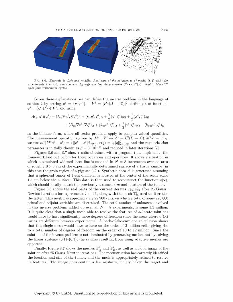
Fig. 8.6. Example 3: Left and middle: Real part of the solution w of model (8.2)–(8.3) forexperiments 2 and 6, characterized by different boundary sources S2(x), S6(x). Right: Mesh T

6

after four refinement cycles.

Given these explanations, we can define the inverse problem in the language ofsection 2 by setting ui = {wi, vi} ∈ V i = [H1(Ω → C)]2, defining test functionsϕi = {ζi, ξi} ∈ V i, and using

A(q;ui)(ϕi) = (Dx∇ui,∇ζi)Ω + (kxui, ζi)Ω +

γ

2(ui, ζi)∂Ω +

1

2(Si, ζi)∂Ω

+ (Dm∇vi,∇ξi)Ω + (kmvi, ξi)Ω +γ

2(vi, ξi)∂Ω − (bxmui, ξi)Ω

as the bilinear form, where all scalar products apply to complex-valued quantities.The measurement operator is given by M i : V i �→ Zi = L2(Σ → C),M iui = vi|Σ,we use mi(M iui − zi) = 1

2‖vi − zi‖2L2(Σ), r(q) = 1

2‖q‖2L2(Ω), and the regularization

parameter is initially chosen as β = 3 · 10−11 and reduced in later iterations [7].Figures 8.6 and 8.7 show results obtained with a program that implements the

framework laid out before for these equations and operators. It shows a situation inwhich a simulated widened laser line is scanned in N = 8 increments over an areaof roughly 8 × 8 cm of the experimentally determined surface of a tissue sample (inthis case the groin region of a pig; see [42]). Synthetic data zi is generated assumingthat a spherical tumor of 1-cm diameter is located at the center of the scene some1.5 cm below the surface. This data is then used to reconstruct the function q(x),which should ideally match the previously assumed size and location of the tumor.

Figure 8.6 shows the real parts of the current iterates u225, u

625 after 25 Gauss–

Newton iterations for experiments 2 and 6, along with the mesh T625 used to discretize

the latter. This mesh has approximately 22,900 cells, on which a total of some 270,000primal and adjoint variables are discretized. The total number of unknowns involvedin this inverse problem, added up over all N = 8 experiments, is some 1.5 million.It is quite clear that a single mesh able to resolve the features of all state solutionswould have to have significantly more degrees of freedom since the areas where ui(x)varies are different between experiments. A back-of-the-envelope calculation showsthat this single mesh would have to have on the order of 2 million cells, giving riseto a total number of degrees of freedom on the order of 10 to 12 million. Since thesolution of the inverse problem is not dominated by generating meshes but by solvingthe linear systems (6.1)–(6.3), the savings resulting from using adaptive meshes areapparent.

Finally, Figure 8.7 shows the meshes Tq11 and T

q25, as well as a cloud image of the

solution after 25 Gauss–Newton iterations. The reconstruction has correctly identifiedthe location and size of the tumor, and the mesh is appropriately refined to resolveits features. The image does contain a few artifacts, mainly below the target and



Fig. 8.7. Example 3: Left and middle: Meshes Tq used to discretize the parameter q(x) after

one and four refinement cycles, respectively. The left mesh is used for Gauss–Newton iterations8–11, the one in the middle for iterations 22–25. Right: Reconstructed parameter q25 after 25Gauss–Newton iterations.

elsewhere deep inside the tissue; this is not overly surprising given that light doesnot penetrate very deep into tissue. However, the main features are clearly correct.(For similar reconstructions, in particular using experimentally measured instead ofsynthetically generated data, see also [40, 42].)

In the case shown, the final mesh has 977 unknowns, of which 438 are constrainedby the condition 0 ≤ q ≤ 2.5 (the upper bound is, in fact, not attained here). Over thecourse of the entire 25 Gauss–Newton iterations, some 9,000 CG iterations were per-formed to solve the Schur complement systems. Since each iteration involves 2N solves

with Ai or AiT , and we also need 2N solves for (6.2)–(6.3) per the Gauss–Newtonstep, this amounts to a total of some 150,000 solutions of the three-dimensional, cou-pled system (8.2)–(8.3) over the course of the entire computation, which took some6 hours on a 2.2-GHz Opteron system; approximately two-thirds of the total computetime was spent on the last four iterations on the finest grid, underlining the claimthat the initial iterations on coarser meshes are relatively cheap.

9. Conclusions. Adaptive meshing strategies have become the state-of-the-arttechnique in solving partial differential equations. However, they are not yet widelyused in solving inverse problems. This may in part be because the numerical solu-tion of inverse problems has been considered more in the context of optimization thandiscretization. Since practical optimization methods are mostly developed in finite di-mensions, the notion that discretizations can change over the course of a computationtherefore doesn’t fit very well into existing algorithms.

To merge these two streams of research, optimization and discretization, we havepresented a framework for the solution of large-scale multiple-experiment inverseproblems that can deal with adaptively changing meshes. Its main features are asfollows:

• formulation in function spaces, allowing for different discretizations in subse-quent steps of Newton-type nonlinear solvers;

• discretization by adaptive finite element schemes, with different meshes forstate and adjoint variables on the one hand and the parameters sought onthe other;

• inclusion of bound constraints with a simple but efficient active set strategy;and

• choice of a formulation that allows for efficient parallelization.This framework has then been applied to some examples showing that inclusion

of bounds can stabilize the identification of a coefficient from noisy data, as well as the



(obvious) fact that measuring more than once can reduce the effects of noise. The lastexample also demonstrated that the framework is applicable to problems of realisticcomplexity beyond mathematical model problems as well.

There are many aspects of our framework that obviously warrant further research:

• More efficient linear solvers. The majority of the compute time is spent oninverting the Schur complement system (6.1) because constructing precondi-tioners for the matrix S is complicated by the fact that its entries are notknown. Attempts to use simpler versions of this matrix to precondition canbe found in [16]. Another possibility is Krylov subspace recycling techniquesusing information from previous Gauss–Newton iterations. This, however,would have to deal with the fact that the matrix S results from discretiza-tions that may change between iterations.

• Rigorous regularization strategies to determine optimal values of β.• Very little theoretical justification, for example, in terms of convergence

proofs, has been presented for the viability of the individual steps of theframework. Such proofs need to address the function-space setting as well asthe variable discretization.

We hope that future research will answer some of these open questions.

Acknowledgments. The author thanks Rolf Rannacher for the encouragementgiven for this research. It is also a pleasure to thank Amit Joshi for the collaborationon optical tomography, from which Example 3 was generated. The author wishes tothank the two anonymous referees whose suggestions have made this a better paper.

REFERENCES

[1] R. Acar, Identification of coefficients in elliptic equations, SIAM J. Control Optim., 31 (1993),pp. 1221–1244.

[2] U. M. Ascher and E. Haber, Grid refinement and scaling for distributed parameter estimationproblems, Inverse Problems, 17 (2001), pp. 571–590.

[3] U. M. Ascher and E. Haber, A multigrid method for distributed parameter estimation prob-lems, ETNA, 15 (2003), pp. 1–12.

[4] W. Bangerth, Adaptive Finite Element Methods for the Identification of Distributed Param-eters in Partial Differential Equations, Ph.D. thesis, University of Heidelberg, 2002.

[5] W. Bangerth, R. Hartmann, and G. Kanschat, deal.II – a general purpose object orientedfinite element library, ACM Trans. Math. Softw., 33 (2007), pp. 24/1–24/27.

[6] W. Bangerth, R. Hartmann, and G. Kanschat, deal.II Differential Equations AnalysisLibrary, Technical Reference. http://www.dealii.org/ (2008).

[7] W. Bangerth and A. Joshi, Adaptive finite element methods for the solution of inverseproblems in optical tomography, Inverse Problems, 24 (2008), 034011.

[8] W. Bangerth and R. Rannacher, Adaptive Finite Element Methods for Differential Equa-tions, Birkhauser Verlag, Basel, 2003.

[9] H. T. Banks and K. Kunisch, Estimation Techniques for Distributed Parameter Systems,Birkhauser, Basel, 1989.

[10] R. Becker, Adaptive Finite Elements for Optimal Control Problems. Habilitation thesis, Uni-versity of Heidelberg, 2001.

[11] R. Becker, H. Kapp, and R. Rannacher, Adaptive finite element methods for optimal con-trol of partial differential equations: Basic concept, SIAM J. Control Optim., 39 (2000),pp. 113–132.

[12] R. Becker and B. Vexler, A posteriori error estimation for finite element discretization ofparameter identification problems, Numer. Math., 96 (2003), pp. 435–459.

[13] H. Ben Ameur, G. Chavent, and J. Jaffre, Refinement and coarsening indicators for adap-tive parametrization: Application to the estimation of hydraulic transmissivities, InverseProblems, 18 (2002), pp. 775–794.

[14] M. Bergounioux, K. Ito, and K. Kunisch, Primal-dual strategy for constrained optimalcontrol problems, SIAM J. Control Optim., 37 (1999), pp. 1176–1194.



[15] L. T. Biegler, O. Ghattas, M. Heinkenschloss, and B. van Bloemen Waanders, eds.,Large-Scale PDE-Constrained Optimization, Lect. Notes Comput. Sci. Eng. 30, Springer,New York, 2003.

[16] G. Biros and O. Ghattas, Parallel Lagrange-Newton-Krylov-Schur methods for PDE-constrained optimization. Part I: The Krylov-Schur solver, SIAM J. Sci. Comput., 27(2005), pp. 687–713.

[17] G. Biros and O. Ghattas, Parallel Lagrange-Newton-Krylov-Schur methods for PDE-constrained optimization. Part II: The Lagrange-Newton solver and its application to op-timal control of steady viscous flow, SIAM J. Sci. Comput., 27 (2005), pp. 714–739.

[18] A. Bjorck, Numerical Methods for Least Squares Problems, SIAM, Philadelphia, 1996.[19] H. G. Bock, Randwertproblemmethoden zur Parameteridentifizierung in Systemen nichtlin-

earer Differentialgleichungen, Bonner Math. Schriften 183, University of Bonn, 1987.[20] L. Borcea, Electrical impedance tomography, Inverse Problems, 18 (2002), pp. R99–R136.[21] L. Borcea and V. Druskin, Optimal finite difference grids for direct and inverse Sturm

Liouville problems, Inverse Problems, 18 (2002), pp. 979–1001.[22] L. Borcea, V. Druskin, and L. Knizhnerman, On the continuum limit of a discrete inverse

spectral problem on optimal finite difference grids, Comm. Pure Appl. Math., 58 (2005),pp. 1231–1279.

[23] J. Carter and C. Romero, Using genetic algorithms to invert numerical simulations, in Pro-ceedings of ECMOR VIII: 8th European Conference on the Mathematics of Oil Recovery,Freiberg, Germany, European Association of Geoscientists and Engineers, 2002, pp. E–45.

[24] Z. Chen and J. Zou, An augmented Lagrangian method for identifying discontinuous param-eters in elliptic systems, SIAM J. Control Optim., 37 (1999), pp. 892–910.

[25] M. J. Dayde, J.-Y. L’Excellent, and N. I. M. Gould, Element-by-element precondition-ers for large partially separable optimization problems, SIAM J. Sci. Comput., 18 (1997),pp. 1767–1787.

[26] F. Dibos and G. Koepfler, Global total variation minimization, SIAM J. Numer. Anal., 37(2000), pp. 646–664.

[27] H. W. Engl, M. Hanke, and A. Neubauer, Regularization of Inverse Problems, KluwerAcademic Publishers, Dordrecht, The Netherlands, 1996.

[28] A. Godavarty, D. J. Hawrysz, R. Roy, and E. M. Sevick-Muraca, The influence of theindex-mismatch at the boundaries measured in fluorescence-enhanced frequency-domainphoton migration imaging, Optics Express, 10 (2002), pp. 653–662.

[29] S. Gutman, Identification of discontinuous parameters in flow equations, SIAM J. ControlOptim., 28 (1990), pp. 1049–1060.

[30] M. Guven, B. Yazici, X. Intes, and B. Chance, An adaptive multigrid algorithm for regionof interest diffuse optical tomography, in Proceedings of the International Conference onImage Processing, 2003, pp. II: 823–826.

[31] M. Guven, B. Yazici, K. Kwon, E. Giladi, and X. Intes, Effect of discretization error andadaptive mesh generation in diffuse optical absorption imaging: I, Inverse Problems, 23(2007), pp. 1115–1133.

[32] M. Guven, B. Yazici, K. Kwon, E. Giladi, and X. Intes, Effect of discretization error andadaptive mesh generation in diffuse optical absorption imaging: II, Inverse Problems, 23(2007), pp. 1135–1160.

[33] E. Haber and U. M. Ascher, Preconditioned all-at-once methods for large, sparse parameterestimation problems, Inverse Problems, 17 (2001), pp. 1847–1864.

[34] E. Haber, U. M. Ascher, and D. Oldenburg, On optimization techniques for solving non-linear inverse problems, Inverse Problems, 16 (2000), pp. 1263–1280.

[35] E. Haber, S. Heldmann, and U. Ascher, Adaptive finite volume methods for distributednon-smooth parameter identification, Inverse Problems, 23 (2007), pp. 1659–1676.

[36] M. Heinkenschloss, Gauss-Newton Methods for Infinite Dimensional Least Squares Problemswith Norm Constraints, Ph.D. thesis, University of Trier, Germany, 1991.

[37] M. Heinkenschloss and L. Vicente, An interface between optimization and application forthe numerical solution of optimal control problems, ACM Trans. Math. Softw., 25 (1999),pp. 157–190.

[38] K. Ito, M. Kroller, and K. Kunisch, A numerical study of an augmented Lagrangian methodfor the estimation of parameters in elliptic systems, SIAM J. Sci. Statist. Comput., 12(1991), pp. 884–910.

[39] C. R. Johnson, Computational and numerical methods for bioelectric field problems, Crit. Rev.BioMedical Engrg., 25 (1997), pp. 1–81.

[40] A. Joshi, W. Bangerth, K. Hwang, J. C. Rasmussen, and E. M. Sevick-Muraca, Fullyadaptive FEM based fluorescence optical tomography from time-dependent measurements



with area illumination and detection, Med. Phys., 33 (2006), pp. 1299–1310.[41] A. Joshi, W. Bangerth, and E. M. Sevick-Muraca, Non-contact fluorescence optical to-

mography with scanning patterned illumination, Optics Express, 14 (2006), pp. 6516–6534.[42] A. Joshi, W. Bangerth, R. Sharma, W. Wang, and E. M. Sevick-Muraca, Molecular

tomographic imaging of lymph nodes with NIR fluorescence, in Proceedings of the IEEEInternational Symposium on Biomedical Imaging, Arlington, VA, 2007, pp. 564–567.

[43] D. W. Kelly, J. P. de S. R. Gago, O. C. Zienkiewicz, and I. Babuska, A posteriorierror analysis and adaptive processes in the finite element method: Part I–error analysis,Internat. J. Numer. Methods Engrg., 19 (1983), pp. 1593–1619.

[44] C. Kravaris and J. H. Seinfeld, Identification of parameters in distributed parameter systemsby regularization, SIAM J. Control Optim., 23 (1985), pp. 217–241.

[45] K. Kunisch, W. Liu, and N. Yan, A posteriori error estimators for a model parameter esti-mation problem, in Proceedings of the ENUMATH 2001 Conference, 2002.

[46] R. Li, W. Liu, H. Ma, and T. Tang, Adaptive finite element approximation for distributedelliptic optimal control problems, SIAM J. Control Optim., 41 (2002), pp. 1321–1349.

[47] R. Luce and S. Perez, Parameter identification for an elliptic partial differential equationwith distributed noisy data, Inverse Problems, 15 (1999), pp. 291–307.

[48] X.-Q. Ma, A constrained global inversion method using an over-parameterised scheme: Appli-cation to poststack seismic data, Geophysics, 66 (2001), pp. 613–626.

[49] D. Meidner and B. Vexler, Adaptive space-time finite element methods for parabolic opti-mization problems, SIAM J. Control Optim., 46 (2007), pp. 116–142.

[50] M. Molinari, B. H. Blott, S. J. Cox, and G. J. Daniell, Optimal imaging with adap-tive mesh refinement in electrical impedence tomography, Physiological Measurement, 23(2002), pp. 121–128.

[51] M. Molinari, S. J. Cox, B. H. Blott, and G. J. Daniell, Adaptive mesh refinement tech-niques for electrical impedence tomography, Physiological Measurement, 22 (2001), pp. 91–96.

[52] J. Nocedal and S. J. Wright, Numerical Optimization, Springer Ser. Oper. Res., Springer,New York, 1999.

[53] M. K. Sen, A. Datta-Gupta, P. L. Stoffa, L. W. Lake, and G. A. Pope, Stochastic reservoirmodeling using simulated annealing and genetic algorithms, SPE Formation Evaluation,(1995), pp. 49–55.

[54] A. Tarantola, Inverse Problem Theory and Methods for Model Parameter Estimation, SIAM,Philadelphia, 2004.

[55] M. Ulbrich, S. Ulbrich, and M. Heinkenschloss, Global convergence of trust-regioninterior-point algorithms for infinite-dimensional nonconvex minimization subject to point-wise bounds, SIAM J. Control Optim., 37 (1999), pp. 731–764.

[56] B. Vexler and W. Wollner, Adaptive finite elements for elliptic optimization problems withcontrol constraints, SIAM J. Control Optim., 47 (2008), pp. 509–534.

[57] C. R. Vogel, Sparse matrix computations arising in distributed parameter identification, SIAMJ. Matrix Anal. Appl., 20 (1999), pp. 1027–1037.

[58] C. R. Vogel, Computational Methods for Inverse Problems, SIAM, Philadelphia, 2002.[59] L. V. Wang, Ultrasound-mediated biophotonic imaging: A review of acousto-optical tomogra-

phy and photo-acoustic tomography, Disease Markers, 19 (2003/2004), pp. 123–138.[60] W. H. Yu, Necessary conditions for optimality in the identification of elliptic systems with

parameter constraints, J. Optim. Theory Appl., 88 (1996), pp. 725–742.

A FRAMEWORK FOR THE ADAPTIVE FINITE ELEMENT …bangerth/publications/2007-si… · ·...

Documents

Transcript of A FRAMEWORK FOR THE ADAPTIVE FINITE ELEMENT …bangerth/publications/2007-si… · ·...