A Forward-Backward Splitting Method with Component-wise ... · A Forward-Backward Splitting Method...
23
A Forward-Backward Splitting Method with Component-wise Lazy Evaluation for Online Structured Convex Optimization * Yukihiro Togari and Nobuo Yamashita † March 28, 2016 Abstract: We consider large-scale optimization problems whose objective functions are expressed as sums of convex functions. Such problems appear in various fields, such as statistics and machine learning. One method for solving such problems is the online gradient method, which exploits the gradients of a few of the functions in the objective function at each iteration. In this paper, we focus on the sparsity of two vectors, namely a solution and a gradient of each function in the objective function. In order to obtain a sparse solution, we usually add the L1 regularization term to the objective function. Then, because the L1 regularization term consists of all decision variables, the usual online gradient methods update all variables even if each gradient is sparse. To reduce the number of computations required for all variables at each iteration, we can employ a lazy evaluation. This only updates the variables corresponding to nonzero components of the gradient, by ignoring the L1 regularization terms, and evaluates the ignored terms later. Because a lazy evaluation does not exploit the information related to all terms at every iteration, the online algorithm using lazy evaluation may converge slowly. In this paper, we describe a forward-backward splitting type method, which exploits the L1 terms corresponding to the nonzero components of the gradient at each iteration. We show that its regret bound is O( √ T ), where T is the number of functions in the objective function. Moreover, we present some numerical experiments using the proposed method, which demonstrate that the proposed method gives promising results. Keywords: online optimization; regret analysis; text classification 1 Introduction In this paper, we consider the following problem: min T ∑ t=1 { f t (x)+ r(x) } , (1) * Technical Report 2016-001, March 27, 2016. † Graduate School of Informatics, Kyoto University, Yoshida-honmachi, Kyoto, 606-8501, Japan. E-mail: [email protected] 1
Transcript of A Forward-Backward Splitting Method with Component-wise ... · A Forward-Backward Splitting Method...

A Forward-Backward Splitting Method with Component-wise
Lazy Evaluation for Online Structured Convex Optimization∗
Yukihiro Togari and Nobuo Yamashita†
March 28, 2016
Abstract: We consider large-scale optimization problems whose objective functionsare expressed as sums of convex functions. Such problems appear in various fields, suchas statistics and machine learning. One method for solving such problems is the onlinegradient method, which exploits the gradients of a few of the functions in the objectivefunction at each iteration.
In this paper, we focus on the sparsity of two vectors, namely a solution and agradient of each function in the objective function. In order to obtain a sparse solution,we usually add the L1 regularization term to the objective function. Then, becausethe L1 regularization term consists of all decision variables, the usual online gradientmethods update all variables even if each gradient is sparse. To reduce the number ofcomputations required for all variables at each iteration, we can employ a lazy evaluation.This only updates the variables corresponding to nonzero components of the gradient,by ignoring the L1 regularization terms, and evaluates the ignored terms later. Becausea lazy evaluation does not exploit the information related to all terms at every iteration,the online algorithm using lazy evaluation may converge slowly.
In this paper, we describe a forward-backward splitting type method, which exploitsthe L1 terms corresponding to the nonzero components of the gradient at each iteration.We show that its regret bound is O(
√T ), where T is the number of functions in the
objective function. Moreover, we present some numerical experiments using the proposedmethod, which demonstrate that the proposed method gives promising results.
Keywords: online optimization; regret analysis; text classification
1 Introduction
In this paper, we consider the following problem:
min
T∑t=1
ft(x) + r(x)
, (1)
∗Technical Report 2016-001, March 27, 2016.†Graduate School of Informatics, Kyoto University, Yoshida-honmachi, Kyoto, 606-8501, Japan. E-mail:
1

where ft : Rn → R(t = 1, . . . , T ) are differentiable convex functions, and r : Rn → R is acontinuous convex function that is not necessarily differentiable. Typical examples of thisproblem appear in machine learning and signal processing. In these examples, ft is regardedas a loss function, such as a logistic loss function ft(x) = log(1 + exp(−bt⟨at, x⟩)) [2, 7] ora hinge loss function ft(x) = [−bt⟨at, x⟩ + 1]+ [4]. Here, (at, bt) ∈ Rn+1 is a pair from thetth sample data. Furthermore, r is a regularization function to avoid over-fitting, such as theL1 regularization term r(x) = λ
∑ni=1 |x(i)| or the L2 regularization term r(x) = λ
2∥x∥2. For
some applications, this may be an indicator function of the feasible set Ω, which is defined by
rΩ(x) =
0 if x ∈ Ω+∞ otherwise.
In this paper, we consider problem (1) under the following circumstances:
(i) Either the upper limit of the summation T is very large, or the functions ft are givenone by one at the tth iteration; that is, the number of functions ft increases with t.
(ii) The gradient ∇ft(x) is sparse; that is, It ≪ n, where It =i∣∣∣∂ft(x)∂x(i) = 0
.
(iii) The function r is decomposable.
In machine learning and statistics, T corresponds to the number of training samples, and ft isa loss function for the tth sample. Therefore, if we have large number of samples, T becomeslarge. When ft is the logistic function given above and some sample data at in ft is sparse,then the gradient of ft is also sparse. Further, if r is the L1 or L2 regularization term, thenr can be decomposed as
r(x) =n∑
i=1
ri(x(i)), (2)
where ri : R → R and x(i) denotes the ith component of the decision variable x. Throughoutthis paper, we assume that r is expressed as (2). We can easily extend the subsequentdiscussions to the case where r is decomposable with respect to blocks of variables, such asthe group lasso.
For problems satisfying (i)-(iii), the online gradient method is useful. This generates asequence of reasonable solutions using only the gradient of ft at the tth iteration [15, 16]. Notethat this is essentially the same as the incremental gradient method [1] and the stochasticgradient method [5, 6]. In this paper, we adopt the online gradient method for the problem(1) satisfying (i)-(iii).
We usually evaluate the online gradient method using a regret, which is defined by
R(T ) =T∑t=1
ft(xt) + r(xt)
−min
x
T∑t=1
ft(x) + r(x)
, (3)
where xt is a sequence generated by the online gradient method. The regret R(T ) is theresidual between the optimum value of (1) and the sum of the values of ft at xt. When
R(T ) satisfies limT→∞R(T )T = 0, we conclude that the online gradient method converges to
an optimal solution.
2
Various online gradient methods have been proposed for problem (1) [14]. When theobjective function consists of non-differentiable functions, such as the L1 regularization term,the online subgradient method for problem (1) updates a sequence as follows [5]:
xt+1 = xt − αt
(∇ft(xt) + ηt
),
where ηt ∈ ∂r(xt) and αt is the stepsize at the tth iteration. If ft is convex, then the regretof the online subgradient method is O(
√T ). Furthermore, if ft is strongly convex, then it
reduces to O(log T ) [14]. However, this algorithm does not fully exploit the structure of r,and it may converge slowly.
The forward-backward splitting (FOBOS) method [8, 9] uses the structure of r. Thisconsists of the gradient method for ft and the proximal point method for r; that is, a sequenceis generated as
xt+1 = argminx
⟨∇ft(xt), x⟩+
1
2αt∥x− xt∥2 + r(x)
. (4)
For given ∇ft(x), we can compute (4) in O(|It|) when ri(x) = 0 for all i. Therefore, when∇ft(x) is sparse as described in (ii), such that |It| ≪ n, we can obtain xt+1 quickly. However,when ri(x) = 0 for all i we require a computation time of O(n) for (4), even if |It| ≪ n.
In order to overcome this drawback, Langford [10] proposed the lazy evaluation method,which defers the evaluation of r in (4) to a later round at most iterations, and exploitsthe information relating to each deferred r all together after a number of iterations. Thistechnique enables us to obtain xt+1 using (4) with only a few computations when ∇ft(x) issparse. However, this method does not fully exploit the information of r at all iterations, andhence its behavior is inferior. Furthermore, even if we employ the L1 regularization term as r,xt cannot be sparse except at the iteration where the deferred evaluations of r are performed.
In this paper, we propose a novel algorithm that conducts the lazy evaluation for ri withrespect to i such that ∇ft(xt) = 0 at each iteration. The usual lazy evaluation process ignoresr for almost all iterations, and evaluates r at a few iterations while updating all components inxt. In contrast, the proposed method conducts the lazy evaluation for the updated variables
x(i)t+1 (i ∈ It) at each iteration. Thus, the proposed method can exploit the full information
given by ri (i ∈ It) at each iteration, and hence the FOBOS method is expected to convergefaster with this technique than with the usual lazy evaluation [10].
The remainder of this paper is organized as follows. In Section 2, we introduce someonline gradient methods and the existing lazy evaluation procedure. In Section 3, we proposea FOBOS method with component-wise lazy evaluation. In Section 4, we prove that the regretof the proposed method is O(
√T ). In Section 5, we present some numerical experiments using
the proposed method. Finally, we provide some concluding remarks in Section 6.Throughout this paper, we employ the following notations. Note that ∥x∥ and ∥x∥p
denote the Euclidean and p-norm of x, respectively. For a differentiable function f : Rn → R,∇(i)f(x) denotes the ith component of ∇f(x). Furthermore, ∂f denotes the subgradient off . The function [·]+ denotes the max function; that is, [a]+ = maxa, 0.
We are aware of that Lipton and Elkan [11] quite recently presented similar idea for theproblem. The idea of the proposed method in this paper were presented in the bachelor thesisof one of the authors of this paper [12]. Further, the regret analysis and numerical experimentsare presented at the meeting of Operations Research Society of Japan [13], which has beenheld in March, 2015.
3
2 Preliminaries
In this section, we introduce the existing online gradient methods, which are the basis of themethod that will be proposed in Section 3.
2.1 Forward-Backward Splitting Method
In this subsection, we introduce some well-known online gradient methods for solving problem(1). The most fundamental algorithm for (1) is the online subgradient method [5], given asfollows.
Algorithm 1 Online Subgradient Method
Step 0: Let x1 ∈ Rn and t = 1.Step 1: Compute the subgradient st ∈ ∂ft(xt) + r(xt).Step 2: Update the sequence by
xt+1 = argminx⟨st, x⟩+1
2αt∥x− xt∥2.
Step 3: Update the stepsize. Set t = t+ 1, and return to Step 1.
When all of the loss functions ft are convex and αt = c√t, the regret (3) of the online
subgradient method is O(√T ) [16], where c is a positive constant. Moreover, when the
functions ft are strongly convex, the regret reduces to O(log T ) [14]. However, this algorithmis inefficient when r is a non-differentiable function, such as the L1 regularization term.
The forward-backward splitting (FOBOS) method [8] is an efficient algorithm for problemswhere r has a special structure.
Algorithm 2 Forward-Backward Splitting Method (FOBOS)
Step 0: Let x1 ∈ Rn and t = 1.Step 1: Set It = i|∇(i)ft(xt) = 0 and update the sequence using the gradient method.
x(i)t+1 =
argminy
αt ∇(i)ft(xt)y +
12(y − x
(i)t )2
if i ∈ It
x(i)t otherwise.
(5)
Step 2: Evaluate ri by the proximal point method.
x(i)t+1 = argminy
ri(y) +
1
2αt(y − x
(i)t+1)
2
for i = 1, . . . , n. (6)
Set t = t+ 1, and return to Step 1.
When ri(x(i)) = λ|x(i)| for a positive constant λ, (6) is rewritten as
x(i)t+1 = sgn
(x(i)t − αt∇(i)ft(xt)
)max
|x(i)t − αt∇(i)ft(xt)| − λαt, 0
for i = 1, . . . , n,
4
where sgn(·) denotes the signature function; that is,
sgn(a) =
+1 if a > 00 if a = 0−1 otherwise .
Moreover, when ri(x(i)) = λ2x
(i)2, (6) is given by
x(i)t+1 =
1
1 + λαtx(i)t − αt
1 + λαt∇(i)ft(xt) for i = 1, ..., n.
The regret obtained by FOBOS has been demonstrated to be O(√
T ). We will assume thatcondition (ii) from the introduction holds. Then, we can note that xit+1 = xit holds in Step 1
for i such that ∇ft(xt) = 0. Therefore, Step 1 only updates x(i) for i ∈ It. However, even if∇ft(xt) is sparse, Step 2 has to update all components when ri(x(i)) = 0 for all i.
2.2 Lazy Evaluations
In this subsection, we introduce the lazy evaluation technique [10], which ignores (6) in FOBOSfor some consecutive iterations. We carry out the ignored updates (6) all together after everyK iterations.
Algorithm 3 FOBOS with Lazy evaluation (L-FOBOS)
Step 0: Let K be a natural number, x1 ∈ Rn, and t = 1.Step 1: Set It = i|∇(i)ft(xt) = 0 and update using the gradient method.
x(i)t+1 =
argminx
αt∇(i)ft(xt)x+ 1
2(x− x(i)t )2
if i ∈ It
x(i)t otherwise.
If t mod K = 0, then set t = t+ 1 and return to Step 1.Otherwise, go to Step 2.
Step 2: Conduct the lazy evaluation for each ri. Let y1 = xt and j = 1.
y(i)j+1 = argminyri(y) +
1
2αt−K+j(y − y
(i)j )2 for i = 1, . . . , n. (7)
If j = j + 1 and j ≤ K, then return to Step 2.Otherwise, set t = t+ 1 and xt = yj and go to Step 1.
In this paper, we refer to the above algorithm as L-FOBOS. Step 1 of L-FOBOS updatesonly xit+1 for i ∈ It using the gradient method. After K consecutive iterations of Step 1, Step2 evaluates the deferred r. Here, Step 2 employs the same stepsizes as the most recent Kiterations in Step 1.
If Step 2 directly calculates (7)K times, then O(Kn) computations are required. However,if r satisfies the following property, then the number of computations required in Step 2 canbe shown to be O(n).
5
Property 1. Let x0 ∈ Rn, and let xt be the sequence obtained by the following formula:
xt+1 = argminx
1
2∥x− xt∥2 + αtr(x)
.
Moreover, let x∗ be the optimal solution of the following optimization problem:
x∗ = argminx
1
2∥x− x0∥2 +
(K∑t=1
αt
)r(x)
.
Then, xK = x∗ holds for any x0.
Note that the L1 and L2 regularization terms and the indicator function for boxed con-straints satisfy the above property [8, Proposition 11].
When r satisfies Property 1, we can aggregate all of the computations needed for Kcalculations (7) into the following O(n) formula:
y(i)K = argminy
ri(y) +
1
2αt(y − x
(i)t )2
(i = 1, . . . , n),
where αt is the sum of the stepsizes of the last K iterations at the tth iteration; that is,αt =
∑tj=t−K+1 αj , with α0 = 0.
By using L-FOBOS, we can update the sequence effectively with respect to the computa-tional complexity. However, the convergence of L-FOBOS might be slower than FOBOS formany problems, because we cannot sufficiently exploit the information given by r. Moreover,we cannot obtain a sparse sequence, even if we set r as the L1 regularization term. Hence,in the next section we will present a novel lazy evaluation technique that can exploit theinformation given by r.
3 FOBOS with Component-wise Lazy Evaluation
As discussed in Section 2, applying the proximal point method to i /∈ It is inefficient for aproblem with sparse gradients. It may not be useful to update the variables without r, as inthe L-FOBOS method. Therefore, we propose the following method, which exploits both thesparsity of gradients and the decomposability of r. Note that the proposed algorithm adopts
the lazy evaluation of ri for x(i)t (i ∈ It) after the gradient method has been used to update
x(i)t .Algorithm 4 is hereafter referred to as CL-FOBOS, where ξ(i) denotes the number of
iterations to elapse since the iteration where x(i) was most recently updated. Note thatL-FOBOS only updates x(i) once every K iterations using the information of r [10], whileCL-FOBOS exploits ri(i ∈ It) at each iteration.
Step 2 of CL-FOBOS requires ξ(i) iterations for i ∈ It. However, we can aggregate allof the necessary computations for Step 2 if r satisfies Property 1 from Section 2. From thispoint on, we assume that r satisfies the following assumption:
Assumption 1. (i) The function r is decomposable with respect to each component of thedecision valuable x.
6
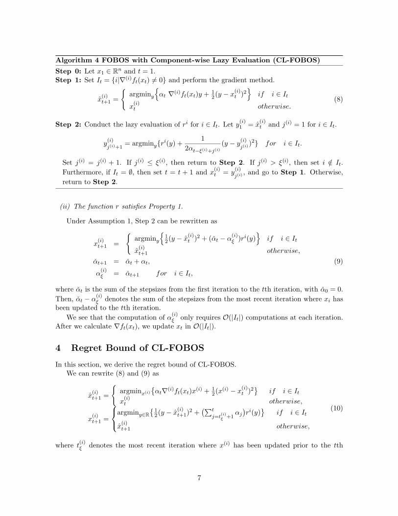
Algorithm 4 FOBOS with Component-wise Lazy Evaluation (CL-FOBOS)
Step 0: Let x1 ∈ Rn and t = 1.Step 1: Set It = i|∇(i)ft(xt) = 0 and perform the gradient method.
x(i)t+1 =
argminy
αt ∇(i)ft(xt)y +
12(y − x
(i)t )2
if i ∈ It
x(i)t otherwise.
(8)
Step 2: Conduct the lazy evaluation of ri for i ∈ It. Let y(i)1 = x
(i)t and j(i) = 1 for i ∈ It.
y(i)
j(i)+1= argminyri(y) +
1
2αt−ξ(i)+j(i)(y − y
(i)
j(i))2 for i ∈ It.
Set j(i) = j(i) + 1. If j(i) ≤ ξ(i), then return to Step 2. If j(i) > ξ(i), then set i /∈ It.
Furthermore, if It = ∅, then set t = t + 1 and x(i)t = y
(i)
j(i), and go to Step 1. Otherwise,
return to Step 2.
(ii) The function r satisfies Property 1.
Under Assumption 1, Step 2 can be rewritten as
x(i)t+1 =
argminy
12(y − x
(i)t )2 + (αt − α
(i)ξ )ri(y)
if i ∈ It
x(i)t+1 otherwise,
αt+1 = αt + αt, (9)
α(i)ξ = αt+1 for i ∈ It,
where αt is the sum of the stepsizes from the first iteration to the tth iteration, with α0 = 0.
Then, αt − α(i)ξ denotes the sum of the stepsizes from the most recent iteration where xi has
been updated to the tth iteration.
We see that the computation of α(i)ξ only requires O(|It|) computations at each iteration.
After we calculate ∇ft(xt), we update xt in O(|It|).
4 Regret Bound of CL-FOBOS
In this section, we derive the regret bound of CL-FOBOS.We can rewrite (8) and (9) as
x(i)t+1 =
argminx(i)
αt∇(i)ft(xt)x
(i) + 12(x
(i) − x(i)t )2
if i ∈ It
x(i)t otherwise,
x(i)t+1 =
argminy∈R12(y − x
(i)t+1)
2 +(∑t
j=t(i)ξ +1
αj
)ri(y)
if i ∈ It
x(i)t+1 otherwise,
(10)
where t(i)ξ denotes the most recent iteration where x(i) has been updated prior to the tth
7

iteration. The regret bound of CL-FOBOS, Rcl(T ), can then written as
Rcl(T ) =T∑t=1
ft(xt) +
n∑i=1
ri(x(i)t )−
T∑t=1
ft(x∗) +
n∑i=1
ri(x(i)∗ ), (11)
where x∗ denotes the optimal solution of problem (1). We will analyze the upper bound of
Rcl(T ), and will show that limT→∞Rcl(T )
T = 0 holds under the following assumption.
Assumption 2. (i) t− t(i)ξ ≤ K holds, where K is a positive constant.
(ii) There exists a positive constant D such that |xt − x∗| ≤ D for t = 1, . . . , T .
(iii) There exists a positive constant G such that supvf∈∂ft(xt) ∥vf∥ ≤ G and supvr∈∂r(xt) ∥vr∥ ≤G for t = 1, . . . , T .
(iv) The stepsize αt is given as αt =α0√t, where α0 is a positive constant.
Assumption 2 (i) ensures that all of the components of xt are updated at least once inevery K iterations. The conditions (ii), (iii), and (iv) of Assumption 2 are assumed in (5) and(6) of the regret analysis of FOBOS. In particular, Assumption 2 (ii) implies the boundedness
of xt, and thus|ri(x(i)t ) − ri(x
(i)∗ )|and
|ri(x(i)t )|
are also bounded. Hence, there exist
positive constants R and S such that
n∑i=1
|ri(x(i)t )− ri(x(i)∗ )| ≤ R for t = 1, . . . , T. (12)
|ri(x(i)t )| ≤ S for i = 1, . . . , n, and t = 1, . . . , T. (13)
Finally, the stepsize given in Assumption 2 (iv) is often employed for online gradient methods.Under Assumptions 1 and 2, we now provide a regret bound for CL-FOBOS.
Theorem 1. Let xt be a sequence generated by CL-FOBOS, and suppose that Assumptions1 and 2 hold. Then, the regret bound of CL-FOBOS is given by
Rcl(T ) =
T∑t=1
ft(xt) +
n∑i=1
ri(x(i)t )−
T∑t=1
ft(x∗) +
n∑i=1
ri(x(i)∗ )
= O(log T ) +O(√T ).
To prove Theorem 1, we use the existing result on the regret bound of FOBOS. Specifically,we consider the sequence xt given by CL-FOBOS (10) as that generated by FOBOS for acertain convex optimization problem.
We first see that (10) is equivalent to
x(i)t+1 = argminx(i)
αt∇(i)ft(xt)x
(i) + αt
n∑i=1
rit(x(i)) +
1
2(x(i) − x
(i)t )2
, (14)
8
where rit : R → R is defined as
rit(y) = c(i)t ri(y),
c(i)t =
∑t
j=t(i)ξ
+1αj
αtif i ∈ It
0 otherwise.
Note that (14) generates the same sequence as (10).The update (14) constitutes the FOBOS procedure for the following problem, with ft and∑n
i=1 rit:
minT∑t=1
ft(x) +
n∑i=1
rit(x). (15)
Note that rit in problem (15) depends on t, whereas r(x) of problem (1) does not. Hereafter,we refer to (14) as Algorithm γ. Because Algorithm γ constitutes the FOBOS procedure forproblem (15), [8] demonstrates that its regret (16) is given by
Rγ(T ) =
T∑t=1
(ft(xt) +
n∑i=1
rit(x(i)t ))−(ft(x∗) +
n∑i=1
rit(x(i)∗ )
)=
T∑t=1
(ft(xt) +
n∑i=1
c(i)t ri(x
(i)t ))−(ft(x∗) +
n∑i=1
c(i)t ri(x
(i)∗ ))
≤ Uγ(T ), (16)
where Uγ(T ) = 2GD+(
D2
2α0+7G2α0
)√T . Note that Rcl(T ) is different from Rγ(T ), whereas
xt in Rcl(T ) is same as that in Rγ(T ). In fact, c(i)t in rit influences Rγ(T ). We will first
evaluate the upper bound of Rcl(T ) by using Rγ(T ).From a simple rearranging, we obtain the upper bound of Rcl(T ) as follows:
Rcl(T ) =
T∑t=1
ft(xt) +
n∑i=1
ri(x(i)t )−
T∑t=1
ft(x∗) +
n∑i=1
ri(x(i)∗ )
≤T∑t=1
(ft(xt) +
∑i∈It
k(i)t ri(x
(i)t ))−(ft(x∗) +
n∑i=1
ri(x(i)∗ ))
+∣∣∣ T∑t=1
n∑i=1
ri(x(i)t )−
T∑t=1
∑i∈It
k(i)t ri(x
(i)t )∣∣∣, (17)
where k(i)t are constants defined by
k(i)t = t− t
(i)ξ . (18)
Throughout the subsequent discussions, let c(i)t be given by
c(i)t =
c(i)t
k(i)t
. (19)
Using these notations, we have the following lemma.
9
Lemma 1. Let xt be a sequence generated by CL-FOBOS, and suppose that Assumptions1 and 2 hold. Then, the following inequality holds:
Rcl(T ) ≤ Uγ(T ) +
T∑t=1
∑i∈It
k(i)t
∣∣∣1− c(i)t
∣∣∣∣∣∣ri(x(i)t )− ri(x(i)∗ )∣∣∣
+∣∣∣ T∑t=1
n∑i=1
ri(x(i)t )−
T∑t=1
∑i∈It
k(i)t ri(x
(i)t )∣∣∣+nKS.
Proof. To prove this lemma, we evaluate the first term of the right-hand side in (17); that is,
T∑t=1
(ft(xt) +
∑i∈It
k(i)t ri(x
(i)t ))−(ft(x∗) +
n∑i=1
ri(x(i)∗ ))
. (20)
First, we obtain that
T∑t=1
n∑i=1
ri(x(i)∗ ) =
n∑i=1
T∑t=1
ri(x(i)∗ )
=n∑
i=1
T(i)ξ∑
t=1
ri(x(i)∗ ) +
n∑i=1
T∑t=T
(i)ξ +1
ri(x(i)∗ )
=
T∑t=1
∑i∈It
k(i)t ri(x
(i)∗ ) +
n∑i=1
T∑t=T
(i)ξ +1
ri(x(i)∗ ) , (21)
where the last equation follows from (18) and the property that ri(x∗) is independent of t.From the conditions (i), (13), and (18) of Assumption 2, we can evaluate the second term in(21) as
n∑i=1
T∑t=T
(i)ξ +1
ri(x(i)∗ ) =
n∑i=1
k(i)T ri(x
(i)∗ )
≥ −K
n∑i=1
|ri(x(i)∗ )|
≥ −nKS.
Moreover, because c(i)t = 0 for i /∈ It, we obtain that
n∑i=1
c(i)t ri(x
(i)t ) =
∑i∈It
c(i)t ri(x
(i)t ). (22)
10
By substituting (21) and (22) into (20), we have that
T∑t=1
(ft(xt) +
∑i∈It
k(i)t ri(x
(i)t ))−(ft(x∗) +
n∑i=1
ri(x(i)∗ ))
=T∑t=1
(ft(xt) +
∑i∈It
k(i)t ri(x
(i)t ))−(ft(x∗) +
∑i∈It
k(i)t ri(x
(i)∗ ))
−n∑
i=1
T∑t=T
(i)ξ +1
ri(x(i)∗ )
≤T∑t=1
(ft(xt) +
n∑i=1
c(i)t ri(x
(i)t ))−(ft(x∗) +
n∑i=1
c(i)t ri(x
(i)∗ ))
+∣∣∣ T∑t=1
∑i∈It
k(i)t ri(x
(i)t )
−T∑t=1
n∑i=1
c(i)t ri(x
(i)t ) +
T∑t=1
n∑i=1
c(i)t ri(x
(i)∗ )−
T∑t=1
∑i∈It
k(i)t ri(x
(i)∗ )∣∣∣+nKS
≤ Uγ(T ) +∣∣∣ T∑t=1
∑i∈It
(k(i)t − c
(i)t )(ri(x
(i)t )− ri(x
(i)∗ ))∣∣∣+nKS, (23)
where the last inequality of (23) follows from (16). Finally, by replacing c(i)t in (23) with c
(i)t
from (19), we obtain
T∑t=1
(ft(xt) +
∑i∈It
k(i)t ri(x
(i)t ))−(ft(x∗) +
n∑i=1
ri(x(i)∗ ))
≤ Uγ(T ) +
T∑t=1
∑i∈It
k(i)t
∣∣∣1− c(i)t
∣∣∣∣∣∣ri(x(i)t )− ri(x(i)∗ )∣∣∣+nKS.
From Lemma 1, we can now obtain the upper bound of the regret Rcl(T ) as
Rcl(T ) ≤ Uγ(T ) + P (T ) +Q(T ) + nKS, (24)
where P (T ) and Q(T ) are defined by
P (T ) =
T∑t=1
∑i∈It
k(i)t
∣∣∣1− c(i)t
∣∣∣∣∣∣ri(x(i)t )− ri(x(i)∗ )∣∣∣. (25)
Q(T ) =∣∣∣ T∑t=1
n∑i=1
ri(x(i)t )−
T∑t=1
∑i∈It
k(i)t ri(x
(i)t )∣∣∣, (26)
respectively. We will now evaluate the upper bounds of P (T ) and Q(T ). For this purpose,
let us first derive an upper bound for the term |1− c(i)t |.
Lemma 2. Suppose that Assumption 2 holds. Then, we have that
|1− c(i)t | ≤ δ(t)
11
for i ∈ It, where δ(t) is given by
δ(t) =
√t− 1 if t ≤ K − 1K−1
2(t−K+1) oterwise.
Proof. From the definitions of c(i)t and c
(i)t , we have for each i ∈ It,∣∣∣1− c
(i)t
∣∣∣ =∣∣∣1− c
(i)t
k(i)t
∣∣∣=
∣∣∣1−∑t
j=t(i)ξ +1
αj
αtk(i)t
∣∣∣. (27)
Note that αj ≥ αt holds for j ≤ t, because it follows from Assumption 2 (iv) that αt =α0√t.
Then, it follows from (18) that∑t
j=t(i)ξ +1
αj
αtk(i)t
≥
∑t
j=t(i)ξ +1
αt
αtk(i)t
=(t− t
(i)ξ )αt
αtk(i)t
= 1. (28)
Moreover, from (27) and (28), we obtain that∣∣∣∣∣1−∑t
j=t(i)ξ +1
αj
αtk(i)t
∣∣∣∣∣ =
∑t
j=t(i)ξ +1
αj
αtk(i)t
− 1
=
∑t
j=t(i)ξ +1
(αj − αt)
αtk(i)t
. (29)
Next, let us consider the upper bound of αj in (29). When t > K − 1, we have that
0 < t−K + 1 ≤ t(i)ξ + 1, from Assumption 2 (i). Then, we have that αj ≤ αt−K+1 holds for
12
j = t(i)ξ + 1, . . . , t, which follows from Assumption 2 (iv). Hence, (29) can be rewritten as∣∣∣∣∣1−
∑t
j=t(i)ξ +1
αj
αtk(i)t
∣∣∣∣∣ =
∑t
j=t(i)ξ +1
(αj − αt)
αtk(i)t
≤
∑t
j=t(i)ξ +1
(αt−K+1 − αt)
αtk(i)t
=k(i)t (αt−K+1 − αt)
αtk(i)t
=(αt−K+1 − αt)
αt
=
(α0√
t−K+1− α0√
t
)α0√t
=
√t−
√t−K + 1√
t−K + 1
=K − 1√
t−K + 1(√t+
√t−K + 1)
≤ K − 1√t−K + 1(2
√t−K + 1)
=K − 1
2(t−K + 1). (30)
On the other hand, when t ≤ K − 1, αj ≤ α0 holds for any j. Then, it then follows from (18)that (29) can be evaluated as∣∣∣∣∣1−
∑t
j=t(i)ξ +1
αj
αtk(i)t
∣∣∣∣∣ =
∑t
j=t(i)ξ +1
(αj − αt)
αtk(i)t
≤
∑t
j=t(i)ξ +1
(α0 − αt)
αtk(i)t
=(α0 − αt)k
(i)t
αtk(i)t
=√t− 1 . (31)
Consequently, we have from (27), (30), and (31) that∣∣1− c
(i)t
∣∣≤ δ(t).
Using Lemma 2, we can give an upper bound for P (T ) as follows.
Lemma 3. Suppose that Assumptions 1 and 2 hold. Then, the following inequality holds:
P (T ) ≤ K(K√K −K + 1)R+
K(K − 1)R
2
(1 + log(T −K + 1)
).
13

Proof. By applying Lemma 2 to the definition (25) of P (T ), we get that
P (T ) =T∑t=1
∑i∈It
k(i)t
∣∣∣1− c(i)t
∣∣∣∣∣∣ri(x(i)t )− ri(x(i)∗ )∣∣∣
≤ KT∑t=1
∑i∈It
∣∣∣1− c(i)t
∣∣∣∣∣∣ri(x(i)t )− ri(x(i)∗ )∣∣∣
≤ KT∑t=1
∑i∈It
δ(t)∣∣∣ri(x(i)t )− ri(x
(i)∗ )∣∣∣
≤ KT∑t=1
n∑i=1
δ(t)∣∣∣ri(x(i)t )− ri(x
(i)∗ )∣∣∣
= K
K−1∑t=1
(√t− 1)
n∑i=1
∣∣∣ri(x(i)t )− ri(x(i)∗ )∣∣∣+K
T∑t=K
K − 1
2(t−K + 1)
n∑i=1
∣∣∣ri(x(i)t )− ri(x(i)∗ )∣∣∣,
where the first inequality follows from Assumption 2 (i). Moreover, by using (12) we havethat
P (T ) ≤ K
K−1∑t=1
(√t− 1)
n∑i=1
∣∣∣ri(x(i)t )− ri(x(i)∗ )∣∣∣+K
T∑t=K
K − 1
2(t−K + 1)
n∑i=1
∣∣∣ri(x(i)t )− ri(x(i)∗ )∣∣∣
≤ KR
K−1∑t=1
(√t− 1) +
K(K − 1)R
2
T∑t=K
1
t−K + 1. (32)
The first term of the right-hand side in (32) can be evaluated as
K−1∑t=1
(√t− 1) ≤
∫ K
1(√t− 1)dt < K
√K −K + 1.
Moreover, the second term of the right-hand side in (32) is bounded above, as
T∑t=K
1
t−K + 1=
T−K+1∑i=1
1
i≤ 1 + log(T −K + 1).
By substituting these two inequalities into (32), we obtain the desired inequality.
Finally, we now derive the upper bound of Q(T ) in (24).
Lemma 4. Let xt be a sequence generated by CL-FOBOS, and suppose that Assumptions1 and 2 hold. Then, it holds that Q(T ) ≤ nKS.
Proof. To simplify, let Q(i)(T ) and Q(i)(T ) be given by
Q(i)(T ) =∣∣∣T
(i)ξ∑
t=1
ri(x(i)t )−
T(i)ξ∑
t=1
κ(i)t ri(x
(i)t )∣∣∣,
Q(i)(T ) =∣∣∣ T∑t=T
(i)ξ +1
ri(x(i)t )∣∣∣,
14
respectively, where T(i)ξ denotes the most recent iteration where x(i) was updated prior to the
T th iteration, and each κ(i)t is given by
κ(i)t =
k(i)t if i ∈ It
0 otherwise.
First, we first show that
n∑i=1
Q(i)(T ) +Q(i)(T )
≥ Q(T ). (33)
From the triangle inequality, we have that
n∑i=1
Q(i)(T ) +Q(i)(T )
=
n∑i=1
∣∣∣T(i)ξ∑
t=1
ri(x(i)t )−
T(i)ξ∑
t=1
κ(i)t ri(x
(i)t )∣∣∣+∣∣∣ T∑
t=T(i)ξ +1
ri(x(i)t )∣∣∣
≥∣∣∣ n∑i=1
T(i)ξ∑
t=1
ri(x(i)t )−
n∑i=1
T(i)ξ∑
t=1
κ(i)t ri(x
(i)t ) +
n∑i=1
T∑t=T
(i)ξ +1
ri(x(i)t )∣∣∣
=∣∣∣ n∑i=1
T∑t=1
ri(x(i)t )−
n∑i=1
T(i)ξ∑
t=1
κ(i)t ri(x
(i)t )∣∣∣.
It follows from the definition of κ(i)t and (18) that
n∑i=1
Q(i)(T ) +Q(i)(T )
≥
∣∣∣ n∑i=1
T∑t=1
ri(x(i)t )−
n∑i=1
T(i)ξ∑
t=1
κ(i)t ri(x
(i)t )∣∣∣
=∣∣∣ T∑t=1
n∑i=1
ri(x(i)t )−
n∑i=1
T∑t=1
κ(i)t ri(x
(i)t )∣∣∣
=∣∣∣ T∑t=1
n∑i=1
ri(x(i)t )−
T∑t=1
n∑i=1
κ(i)t ri(x
(i)t )∣∣∣
=∣∣∣ T∑t=1
n∑i=1
ri(x(i)t )−
T∑t=1
∑i∈It
k(i)t ri(x
(i)t )∣∣∣.
We see that the last term is Q(T ), and hence we have that∑n
i=1
Q(i)(T )+Q(i)(T )
≥ Q(T ).
From this inequality, we may evaluate both Q(i)(T ) and Q(i)(T ) to obtain the upper boundof Q(T ).
First, we first define some notations to be employed in these evaluations. Let l(i,m) be
the iteration at which x(i) has been updated m times with l(i, 0) = 0. Furthermore, let M(i)T
denote the number times that x(i) has been updated by the T th iteration. Note that M(i)T
satisfiesl(i,M
(i)T ) = T
(i)ξ , (34)
15
because the most recent iteration at which x(i) has been updated before the T th iteration is
the same as that at which x(i) has been updated M(i)T times. We consider the properties of
the sequence x(i)t with respect to l(i,m) and M(i)T . Because x(i)t is the sequence generated
by (10), x(i)t is only updated when i ∈ It. Therefore we have that
i ∈ It ⇔ t ∈l(i,m)
∣∣ m = 1, . . . ,M(i)T
, (35)
i /∈ It ⇔ t ∈l(i,m) + 1, . . . , l(i,m+ 1)− 1
∣∣ m = 1, . . . ,M(i)T
. (36)
In particular, we have that x(i)t+1 = x
(i)t holds at each iteration such that i /∈ It. Then, it
follows from (36) that
x(i)t = x
(i)l(i,m+1) (t = l(i,m) + 1, . . . , l(i,m+ 1)). (37)
Now, using these notations we evaluate will Q(i)(T ) and Q(i)(T ). First, we can use (35)
to rewrite Q(i)(T ) as
Q(i)(T ) =∣∣∣T
(i)ξ∑
t=1
ri(x(i)t )−
T(i)ξ∑
t=1
∑i∈It
k(i)t ri(x
(i)t )∣∣∣
=∣∣∣M(i)
T −1∑m=0
l(i,m+1)∑t=l(i,m)+1
ri(x(i)t )−
M(i)T −1∑m=0
k(i)l(i,m+1)r
i(x(i)l(i,m+1))
∣∣∣ .Here, note that k
(i)l(i,m+1)r
i(x(i)l(i,m+1)) =
∑l(i,m+1)t=l(i,m)+1 r
i(x(i)l(i,m+1)), because k
(i)l(i,m+1) = l(i,m +
1)− l(i,m). Therefore, we have that
Q(i)(T ) =∣∣∣M(i)
T −1∑m=0
l(i,m+1)∑t=l(i,m)+1
ri(x(i)t )−
M(i)T −1∑m=0
l(i,m+1)∑t=l(i,m)+1
ri(x(i)l(i,m+1))
∣∣∣= 0, (38)
where the last equation follows from (37).On the other hand, from conditions (i) and (13) of Assumption 2 we have that
Q(i)(T ) =∣∣∣ T∑t=T
(i)ξ +1
ri(x(i)t )∣∣∣
≤∣∣∣ T∑t=T−K+1
ri(x(i)t )∣∣∣
≤ KS. (39)
Furthermore, from (33), (38), and (39), we obtain that Q(T ) ≤ nKS.
Proof of Theorem 1. It is obvious that Theorem 1 follows from Lemma 3, Lemma 4,(16), and (24).
16
Theorem 1 yields that limT→∞Rcl(T )
T = 0.We can regard CL-FOBOS as not only an online gradient method, but also as a stochastic
gradient method for the following stochastic programming problem:
min E(θ(x, z)
), (40)
where z is a random variable, and θ is the loss function with respect to z and a parameter x.Problem (40) is approximately equivalent to the following problem:
min ϕ(x) ≡ 1
T
T∑t=1
θ(x, zt), (41)
where zt represents a random variable for each sample. Now, we obtain the following theoremin a way similar to [15].
Theorem 2. Let xt be the sequence generated by CL-FOBOS for problem (41), and supposethat Assumptions 1 and 2 hold. Then, we have that
limT→∞
E[ϕ( 1T
T∑t=1
xt
)]−ϕ∗ = 0,
where ϕ∗ is the optimal value of problem (40).
5 Numerical Experiments
In this section, we present some numerical results using CL-FOBOS in order to verify itsefficiency. The experiments are carried out on a machine with a 1.7 GHz Intel Core i7 CPUand 8 GB memory, and we implement all codes in C++. We set the initial point x1 to 0 inall experiments.
We compare the performance of CL-FOBOS with L-FOBOS [10] for binary classificationproblems. We use the logistic function ft(x) = log
(1 + exp(−bt⟨at, x⟩)
)and the L1 regular-
ization term r(x) = λ∑n
i=1 |x(i)|, where λ is a positive constant that controls the sparsity ofsolutions, and (at, bt) denotes the tth sample data.
We use an Amazon review dataset, called the Multi-Domain Sentiment Dataset [3], forthe experiments. This dataset contains many merchandise reviews from Amazon.com. Weattempt to divide the reviews into two classes, those expressing positive impressions of themerchandises and those that are negative.
The data for the tth review is composed of a vector at ∈ Rn and a label bt ∈ +1,−1.The vector at ∈ Rn is constructed by the so-called ”Bag-of-Words” process, and a
(i)t represents
the number of times that the word represented by i appears in the tth sentence of the review.Hence, at is regarded as a feature vector of the tth sentence of the review. Meanwhile, thelabel bt indicates the evaluation of the merchandise given by the author of the tth review,where ” + 1” represents a positive impression and ”− 1” represents a negative one.
In the experiments, we only use the ”Book” domain from the dataset. The book domainis comprised of 4,465 samples, and the total number of words in all samples is 332,440. Eachfeature vector at(t = 1, . . . ,M) contains at least 11 (at most 5,412) nonzero elements, andthe average number of nonzero elements is 228.
17
The number of samples, 4,465, seems small for comparing online gradient methods. There-fore, we constructed a large dataset using the 4, 465 samples. That is, we randomly choose100, 000 samples from the original 4,465, and we employed this as the dataset for the experi-ments. We compare CL-FOBOS with L-FOBOS in the following four aspects: the average ofthe total loss defined in (42), the rate of correct estimations, the number of nonzero compo-nents in xt, and the run time.
R(T ) =
∑Tt=1
ft(xt) +
∑ni=1 r
(i)(xit)
T. (42)
Note that R(T ) represents a kind of the regret R(T ). The rate of correct estimations is definedas follows. We estimate the class of a sample at each iteration using ⟨at, xt⟩, and then countthe number of correct estimations; that is, the number of samples t such that bt⟨at, xt⟩ > 0.The rate of correct estimations is then the number of correct estimations divided by thenumber of samples that have been observed.
We tested both methods with αt =α0√t, where α0 denotes the initial stepsize, and is set
between 0.005 and 1.0 with width of 0.005. We present the results achieved by each methodwith the best choice of α0; that is, we choose α0 such that smallest R(T ) is obtained.
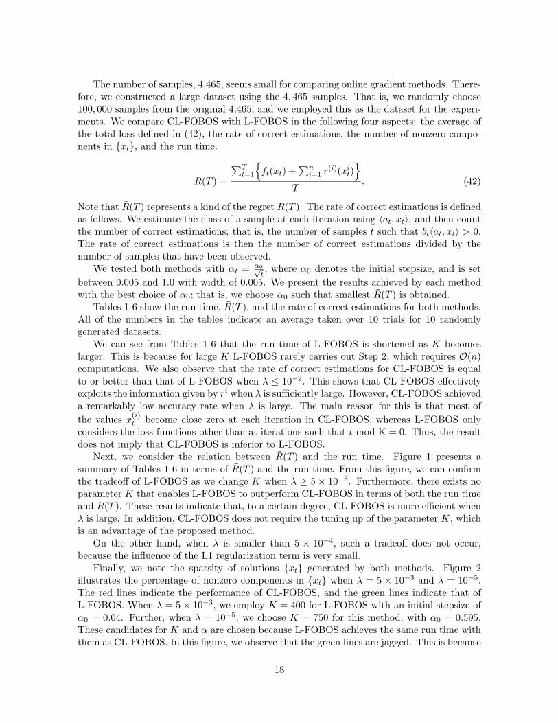
Tables 1-6 show the run time, R(T ), and the rate of correct estimations for both methods.All of the numbers in the tables indicate an average taken over 10 trials for 10 randomlygenerated datasets.
We can see from Tables 1-6 that the run time of L-FOBOS is shortened as K becomeslarger. This is because for large K L-FOBOS rarely carries out Step 2, which requires O(n)computations. We also observe that the rate of correct estimations for CL-FOBOS is equalto or better than that of L-FOBOS when λ ≤ 10−2. This shows that CL-FOBOS effectivelyexploits the information given by ri when λ is sufficiently large. However, CL-FOBOS achieveda remarkably low accuracy rate when λ is large. The main reason for this is that most of
the values x(i)t become close zero at each iteration in CL-FOBOS, whereas L-FOBOS only
considers the loss functions other than at iterations such that t mod K = 0. Thus, the resultdoes not imply that CL-FOBOS is inferior to L-FOBOS.
Next, we consider the relation between R(T ) and the run time. Figure 1 presents asummary of Tables 1-6 in terms of R(T ) and the run time. From this figure, we can confirmthe tradeoff of L-FOBOS as we change K when λ ≥ 5 × 10⁻³. Furthermore, there exists noparameter K that enables L-FOBOS to outperform CL-FOBOS in terms of both the run timeand R(T ). These results indicate that, to a certain degree, CL-FOBOS is more efficient whenλ is large. In addition, CL-FOBOS does not require the tuning up of the parameter K, whichis an advantage of the proposed method.
On the other hand, when λ is smaller than 5 × 10⁻⁴, such a tradeoff does not occur,because the influence of the L1 regularization term is very small.
Finally, we note the sparsity of solutions xt generated by both methods. Figure 2illustrates the percentage of nonzero components in xt when λ = 5 × 10⁻³ and λ = 10−5.The red lines indicate the performance of CL-FOBOS, and the green lines indicate that ofL-FOBOS. When λ = 5× 10⁻³, we employ K = 400 for L-FOBOS with an initial stepsize ofα0 = 0.04. Further, when λ = 10−5, we choose K = 750 for this method, with α0 = 0.595.These candidates for K and α are chosen because L-FOBOS achieves the same run time withthem as CL-FOBOS. In this figure, we observe that the green lines are jagged. This is because
18

Table 1: Results for each algorithm, λ = 10−1
Algorithm Name α0 Run Time R(T ) Rate of Right Estimations
L-FOBOS (K = 100) 0.005 2.00 0.708 0.533L-FOBOS (K = 500) 0.005 1.0 0.759 0.548L-FOBOS (K = 1000) 0.005 0.9 0.818 0.560CL-FOBOS 0.005 0.95 0.694 0.526
Table 2: Results for each algorithm, λ = 10−2
Algorithm Name α0 Run Time R(T ) Rate of Right Estimations
L-FOBOS (K = 100) 0.03 2.15 0.646 0.737L-FOBOS (K = 500) 0.015 1.05 0.662 0.726L-FOBOS (K = 1000) 0.01 0.95 0.673 0.719CL-FOBOS 0.03 1.2 0.645 0.738
Table 3: Results for each algorithm, λ = 5× 10⁻³
Algorithm Name α0 Run Time R(T ) Rate of Right Estimations
L-FOBOS (K = 100) 0.06 2.15 0.599 0.788L-FOBOS (K = 500) 0.035 0.9 0.612 0.780L-FOBOS (K = 1000) 0.025 0.8 0.625 0.774CL-FOBOS 0.055 1.05 0.601 0.787
Table 4: Results for each algorithms, λ = 5× 10⁻⁴
Algorithm Name α0 Run Time R(T ) Rate of Right Estimations
L-FOBOS (K = 100) 0.155 3.15 0.4199 0.906L-FOBOS (K = 500) 0.155 1.3 0.4199 0.906L-FOBOS (K = 1000) 0.155 1.0 0.421 0.905CL-FOBOS 0.155 1.25 0.421 0.905
Table 5: Results for each algorithm, λ = 10−5
Algorithm Name α0 Run Time R(T ) Rate of Right Estimations
L-FOBOS (K = 100) 0.595 5.00 0.1514 0.981L-FOBOS (K = 500) 0.595 1.45 0.1514 0.981L-FOBOS (K = 1000) 0.595 1.00 0.1514 0.9809CL-FOBOS 0.595 1.00 0.152 0.9808
19
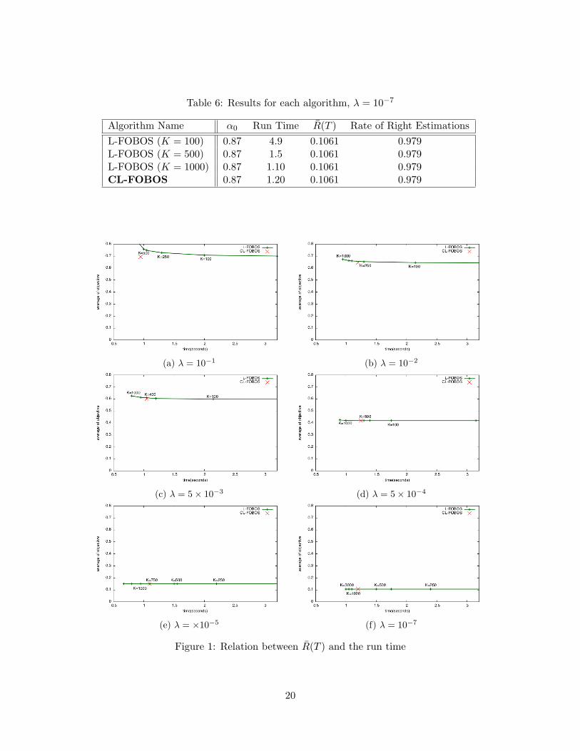
Table 6: Results for each algorithm, λ = 10−7
Algorithm Name α0 Run Time R(T ) Rate of Right Estimations
L-FOBOS (K = 100) 0.87 4.9 0.1061 0.979L-FOBOS (K = 500) 0.87 1.5 0.1061 0.979L-FOBOS (K = 1000) 0.87 1.10 0.1061 0.979CL-FOBOS 0.87 1.20 0.1061 0.979
(a) λ = 10−1 (b) λ = 10−2
(c) λ = 5× 10⁻³ (d) λ = 5× 10⁻⁴
(e) λ = ×10−5 (f) λ = 10−7
Figure 1: Relation between R(T ) and the run time
20
(a) λ = 5× 10⁻³ (b) λ = 10−5
Figure 2: The number of nonzero components in xt
xt becomes radically sparse when t mod K = 0, on account of the lazy evaluation.In particular, when λ = 5× 10⁻³ the solution xt obtained by L-FOBOS becomes approxi-
mately zero at such iterations. Meanwhile, when we set λ = 10−5, we see that both methodsgenerate more dense solutions, because the L1 regularization is almost ignored.
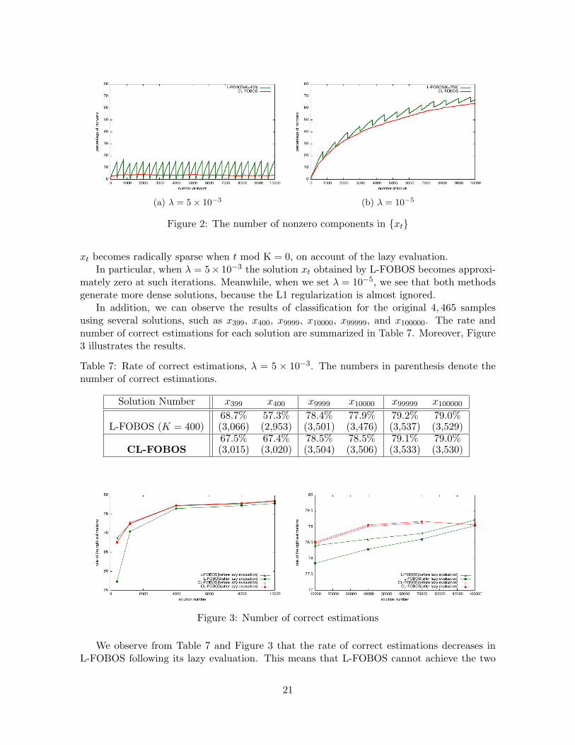
In addition, we can observe the results of classification for the original 4, 465 samplesusing several solutions, such as x399, x400, x9999, x10000, x99999, and x100000. The rate andnumber of correct estimations for each solution are summarized in Table 7. Moreover, Figure3 illustrates the results.
Table 7: Rate of correct estimations, λ = 5 × 10⁻³. The numbers in parenthesis denote thenumber of correct estimations.
Solution Number x399 x400 x9999 x10000 x99999 x100000
L-FOBOS (K = 400)68.7%(3,066)
57.3%(2,953)
78.4%(3,501)
77.9%(3,476)
79.2%(3,537)
79.0%(3,529)
CL-FOBOS67.5%(3,015)
67.4%(3,020)
78.5%(3,504)
78.5%(3,506)
79.1%(3,533)
79.0%(3,530)
Figure 3: Number of correct estimations
We observe from Table 7 and Figure 3 that the rate of correct estimations decreases inL-FOBOS following its lazy evaluation. This means that L-FOBOS cannot achieve the two
21

aims of generating sparse solutions and minimizing the total loss simultaneously. On theother hand, CL-FOBOS is well-balanced. That is, it always creates sparse solutions, and itsaccuracy is improved as it observes samples.
In conclusion, we confirm that the proposed method, CL-FOBOS, is more efficient forproblems that are strongly influenced by the function r.
6 Conclusion
In this paper, we have proposed a novel algorithm, CL-FOBOS, for large-scale problems withsparse gradients. Furthermore, we have derived a bound on the regret of CL-FOBOS. Finally,we confirmed the efficiency of the proposed method using numerical experiments.
As a direction for future work, it would be worth investigating a reasonable stepsize ruleto be determined before CL-FOBOS starts.
References
[1] Bertsekas, P, D. : Incremental Gradient, Subgradient, and Proximal Methods for ConvexOptimization: A Survey, Lab. for information and decision systems report LIDSP-2848,MIT, pp.1-38, 2010.
[2] Bishop, C. : Pattern Recognition and Machine Learning, Springer-Verlag New York, 2006.
[3] Blitzer, J., Dredze, M., Pereira, F. : Domain Adaptation for Sentiment Classification, Inproceedings of the 45th annual meeting of the association of computational linguistics, pp.440-447, 2007.
[4] Blondel, M., Seki, K., Uehara, K. : Block Coordinate Descent Algorithms for Large-scaleSparse Multiclass Classification, The journal of machine learning research volume 93 , pp.31-52, 2013.
[5] Bottou, L. : Online Algorithms and Stochastic Approximations, Online learning and neuralnetworks, pp. 9-42, 1998.
[6] Cesa-Bianchi, N. : Analysis of Two Gradient-based Algorithms for On-line Regression,Journal of computer and system sciences volume 59, pp. 392-411, 1999.
[7] Dredze, M., Crammer, K., Pereira. : Confidence-weighted Linear Classification, Proceed-ings of international conference on machine learning, pp. 264-271, 2008.
[8] Duchi, J., Singer, Y. : Efficient Online and Batch Learning Using Forward BackwardSplitting, The journal of machine learning research volume 10 , pp. 2899-2934, 2009.
[9] Duchi, J., Shalev-Shwartz, S., Singer, Y., Tewari, A. : Composite Objective Mirror De-scent, Conference on learning theory (COLT), pp. 14-26, 2010.
[10] Langford, J., Li, L., Zhang, T. : Sparse Online Learning via Truncated Gradient, Thejournal of machine learning research volume 10 , pp. 777-801, 2009.
22
[11] Lipton, Z., Elkan, C. : Efficient Elastic Net Regularization for Sparse Linear Models,arXiv:1505.06449, 24 May 2015.
[12] Togari, Y., Yamashita, N. : Regret Analysis of Online Optimization Algo-rithm that performs Lazy Evaluation, Bachelor thesis, Kyoto University, March2014, http://www-optima.amp.i.kyoto-u.ac.jp/papers/bachelor/2014_bachelor_
togari.pdf [publish in Japanese].
[13] Togari, Y., Yamashita, N. : Regret Analysis of Forward-Backward Splitting Method withComponent-wise Lazy Evaluation, In Proceedings of the Spring Meeting of the OperationsResearch Society of Japan, 2015 [publish in Japanese].
[14] Shalev-Shwartz, S. : Online Learning and Online Convex Optimization, Foundations andtrends in machine learning volume 4, no 2 , pp. 107-194, 2011.
[15] Xiao, L. : Dual Averaging Methods for Regularized Stochastic Learning and Online Op-timization, The journal of machine learning research volume 11, pp. 2543-2596, 2010.
[16] Zinkevich, M. : Online Convex Programming and Generalized Infinitesimal GradientAscent, Proceedings of the twentieth international conference on machine learning (ICML)pp. 928-936, 2003.
23