A force method model for dynamic analysis of flat-sag cable...
14
Shock and Vibration 16 (2009) 623–635 623 DOI 10.3233/SAV-2009-0493 IOS Press A force method model for dynamic analysis of flat-sag cable structures Xing Ma and John W. Butterworth ∗ Department of Civil and Environmental Engineering, University of Auckland, Private bag 92019, Auckland 1142, New Zealand Received 21 September 2008 Revised 20 December 2008 Abstract. A new force method is proposed for analysing the dynamic behaviour of oscillating cables with small sags. The accepted dynamic model of such cables reduces to a partial differential equation (the equation of motion) and an integral equation (the compatibility equation). In the paper, D’Alembert’s travelling wave solution is applied to the partial differential equation (PDE). Substituting the solution into the compatibility and boundary conditions, the governing equation is obtained in terms of the dynamic tension increment. This equation has been named the force method dynamic equation (FMDE). In this way the infinite-degree-of-freedom dynamic system is effectively simplified to a system with only one unknown. Explicit solutions for both single-span and multi-span cable systems are derived. The natural frequencies obtained from the FMDE are shown to be identical to those deduced using the conventional displacement method (DM). Nonlinear governing equations are developed by considering the effect of quadratic and cubic displacement terms. Finally, two examples are presented to illustrate the accuracy of the proposed force method for single and multi-span cable systems subjected to harmonic forces. Keywords: Force method model, vibration, cable structure, nonlinear analysis, multi-span cable 1. Introduction Cables and cable suspended structures have a wide range of practical applications in both the civil and electrical engineering industries, where their dynamic behaviour is often of crucial importance. The required dynamic analyses have most frequently been carried out in the time domain and based on the displacement method (DM). The prominent linear theory developed by Irvine [4] describes the in-plane and out-of-plane small amplitude free vibration of a suspended elastic cable with small sag. The finite element method has also been used for forced vibration response analysis [7]. However, for cables with complex dynamic geometry, the method needs a quantity of pre-stressed link elements or curved cable elements. To reduce the number of degrees of freedom, low order linear modes are employed to synthesise the dynamic curve of the cable, based on which, discretised models with 2 to 4 displacement modes (d.o.f) have been applied to dynamic analysis of cable-stayed structures [1,9,10]. Unfortunately, in some complex circumstances, the conventional displacement method using a few linearised mode functions may lead to inaccurate response prediction. As a new research approach, Ni, Lou and Ko [8] developed a hybrid pseudo-force/Laplace transform method for transient response of suspended cables. In practical applications, the force method is an ideal structural analysis tool when dealing with pre-stressed structures. You [12] employed the force method to optimise a guyed mast. However, there is no literature available on the use of the force method in dynamic analysis. In dynamic analysis of shallow cables with sag-span ratios smaller than 1/8, the component of additional dynamic tension may be assumed constant in the chord direction if the ∗ Corresponding author. Tel.: +64 9 3737599 88154; E-mail: [email protected]. ISSN 1070-9622/09/$17.00 2009 – IOS Press and the authors. All rights reserved
Transcript of A force method model for dynamic analysis of flat-sag cable...
Shock and Vibration 16 (2009) 623–635 623DOI 10.3233/SAV-2009-0493IOS Press
A force method model for dynamic analysisof flat-sag cable structures
Xing Ma and John W. Butterworth∗Department of Civil and Environmental Engineering, University of Auckland, Private bag 92019, Auckland 1142,New Zealand
Received 21 September 2008
Revised 20 December 2008
Abstract. A new force method is proposed for analysing the dynamic behaviour of oscillating cables with small sags. Theaccepted dynamic model of such cables reduces to a partial differential equation (the equation of motion) and an integral equation(the compatibility equation). In the paper, D’Alembert’s travelling wave solution is applied to the partial differential equation(PDE). Substituting the solution into the compatibility and boundary conditions, the governing equation is obtained in terms ofthe dynamic tension increment. This equation has been named the force method dynamic equation (FMDE). In this way theinfinite-degree-of-freedom dynamic system is effectively simplified to a system with only one unknown. Explicit solutions forboth single-span and multi-span cable systems are derived. The natural frequencies obtained from the FMDE are shown to beidentical to those deduced using the conventional displacement method (DM). Nonlinear governing equations are developed byconsidering the effect of quadratic and cubic displacement terms. Finally, two examples are presented to illustrate the accuracyof the proposed force method for single and multi-span cable systems subjected to harmonic forces.
Keywords: Force method model, vibration, cable structure, nonlinear analysis, multi-span cable
1. Introduction
Cables and cable suspended structures have a wide range of practical applications in both the civil and electricalengineering industries, where their dynamic behaviour is often of crucial importance. The required dynamic analyseshave most frequently been carried out in the time domain and based on the displacement method (DM). The prominentlinear theory developed by Irvine [4] describes the in-plane and out-of-plane small amplitude free vibration of asuspended elastic cable with small sag. The finite element method has also been used for forced vibration responseanalysis [7]. However, for cables with complex dynamic geometry, the method needs a quantity of pre-stressed linkelements or curved cable elements. To reduce the number of degrees of freedom, low order linear modes are employedto synthesise the dynamic curve of the cable, based on which, discretised models with 2 to 4 displacement modes(d.o.f) have been applied to dynamic analysis of cable-stayed structures [1,9,10]. Unfortunately, in some complexcircumstances, the conventional displacement method using a few linearised mode functions may lead to inaccurateresponse prediction. As a new research approach, Ni, Lou and Ko [8] developed a hybrid pseudo-force/Laplacetransform method for transient response of suspended cables.
In practical applications, the force method is an ideal structural analysis tool when dealing with pre-stressedstructures. You [12] employed the force method to optimise a guyed mast. However, there is no literature availableon the use of the force method in dynamic analysis. In dynamic analysis of shallow cables with sag-span ratiossmaller than 1/8, the component of additional dynamic tension may be assumed constant in the chord direction if the
∗Corresponding author. Tel.: +64 9 3737599 88154; E-mail: [email protected].
ISSN 1070-9622/09/$17.00 2009 – IOS Press and the authors. All rights reserved

624 X. Ma and J.W. Butterworth / A force method model for dynamic analysis of flat-sag cable structures
x yz
q(x,t)
l
Fig. 1. Model of a suspended cable.
longitudinal inertia forces are omitted [4,6,9,11,13]. Thus there is only one unknown in the governing equation if theforce method is employed, offering the possibility of reducing the infinite-degree-of-freedom system (deformationmethod model) to a single-degree-freedom system (force method model) without loss of precision.
For an oscillating shallow cable, the dynamic model reduces to a partial differential equation (equation of motion)and an integral equation (compatibility condition). There are two normal methods for PDE solving [5]: the stationarywave method and the travelling wave method. The stationary wave method is applicable to finite length cables, wherea series solution for displacement response can be achieved. This approach is also known as the mode superpositionmethod. However, there is a relatively simple integral formula for displacement response which may be derivedbased on the travelling wave method. In this paper, in order to employ the travelling wave method to solve the PDE,the support reaction forces are considered as excitations, allowing D’Alembert’s solution to be used. Substituting thesolution into the compatibility and boundary condition equations leads to the governing equation expressed in termsof dynamic tension – in which form it has been given the name force method dynamic equation (FMDE). Consideringthe quadratic and cubic terms of the dynamic displacements, nonlinear governing equations are developed. In thisway the infinite-degree-of-freedom dynamic system is reduced to a single-degree-of-freedom system.
2. Linearised undamped model for a single-span cable
2.1. Equation of motion and D’Alembert solution
Consider a transversely loaded single cable spanning a distance l, as shown in Fig. 1. For an undamped verticallyoscillating shallow cable, the linearised equation of motion is [4].
H∂2w
∂x2+ h
d2z
dx2+ q = m
∂2w
∂t2(1)
where m is the mass density; H and h(t) are respectively the horizontal components of static tension and theincrement of dynamic tension; x is the axial coordinate; w(x, t), q(x, t) are respectively the dynamic displacementresponse and excitation load in the z direction. z(x) is the static equilibrium curve of the cable under static gravityloading (q = 0).
Considering support reaction forces as excitations, Eq. (1) is then rewritten as
∂2w
∂t2= a2 ∂
2w
∂x2+ F (x, t) (2)
where
F (x, t) ={
hm
d2zdx2 + f1δ(x)+f2δ(x−l)+q
m0 � x � l and t � 0
0 others(3)
and
a =√
H/m (4)
If the static equilibrium load includes only the self-weight of the system, we get
X. Ma and J.W. Butterworth / A force method model for dynamic analysis of flat-sag cable structures 625
d2z
dx2= −mg
H(5)
f1(t), f2(t) are the support reaction forces and δ(x) is the unit impulse or Dirac delta function, defined as
δ(x) ={ ∞ x = 0
0 x �= 0 and∫ +∞−∞ δ(x)dx = 1 (6)
The D’Alembert solution to Eq. (2) with initial displacement and velocity of zero is
w(x, t) =12a
∫ t
0
∫ x+a(t−τ)
x−a(t−τ)
F (ξ, τ)dξdτ (7)
2.2. Boundary conditions
The boundary conditions are
w(0, t) = w(l, t) = 0 (8)
and
dw(0, t)dt
=dw(l, t)
dt= 0 (9)
Substituting Eq. (7) into Eq. (9) and changing the integral sequence, we get
a
∫ t
t−l/a
{q [a(t− τ), τ ] − mg
Hh(τ)
}dτ + f1(t) + f2
(t− l
a
)= 0 (10a)
and
a
∫ t
t−l/a
{q [l − a(t− τ), τ ] − mg
Hh(τ)
}dτ + f2(t) + f1
(t− l
a
)= 0 (10b)
where the support forces may be expressed as
f1(t) =
{0 t < 0
−f2(t− la ) + a
∫ t
t−l/a
{mgH h(τ) − q [a(t− τ), τ ]
}dτ t � 0 (11a)
f2(t) =
{0 t < 0
−f1(t− la ) + a
∫ t
t−l/a
{mgH h(τ) − q [l − a(t− τ), τ ]
}dτ t � 0 (11b)
Differentiating Eq. (7) with respect to x and substituting x = 0, we get
∂w
∂x(0, t) =
12am
{∫ t
t−l/a
q [a(t− τ), τ ] dτ − mg
H
∫ t
t−l/a
h(τ)dτ − 1af1(t) +
1af2
(t− l
a
)}(12)
Considering Eq. (11a), and recalling a =√
H/m, Eq. (12) may be rewritten as
∂w
∂x(0, t) = −f1(t)
H(13)
Similarly, for x = l, we have
∂w
∂x(l, t) =
f2(t)H
(14)
Equations (13) and (14) show that the dynamic rotational displacements at the cable ends are equal to the ratiosbetween dynamic vertical support forces and the static horizontal tension.
626 X. Ma and J.W. Butterworth / A force method model for dynamic analysis of flat-sag cable structures
2.3. Force method dynamic equation (FMDE)
When oscillating with small amplitude, the displacement compatibility equation of the cable is [4]
h = −EA
le
∫ l
0
d2z
dx2wdx =
EA
le
mg
H
∫ l
0
wdx (15)
where le, l, E, and A are respectively curve length, chord length, elastic modulus and cross sectional area of thecable.
Integrating Eq. (1) with respect to x in domain (0, l), and considering Eqs (8), (13), (14) and (15), leads to thegoverning equation of the system expressed in terms of the dynamic tension increment,
d2h
dt2+ η2h =
η2
r1
[f1 + f2 +
∫ l
0
q(x, t)dx
](16a)
where
η2 =lmg2EA
leH2, r1 =
mgl
H,
and f1(t), f2(t) may be obtained through Eq. (11).Equation (16a) is the force method dynamic equation (FMDE) for oscillating cables. The explicit solution of
Eq. (16a) with initial displacement and velocity of zero may be expressed as
h(t) =1η
∫ t
0
F (τ) sin(ηt− ητ)dτ (16b)
where
F (t) =η2
r1
[f1 + f2 +
∫ l
0
q(x, t)dx
].
Equation (16b) is known as the Duhamel integral equation and may be evaluated numerically using the proceduredescribed in [3].
2.4. Free vibration equation
Substituting Eq. (11) into Eq. (16a) and assuming q(x,t)=0, we get
d2h
dt2+ η2h =
η2
r1
{2r1
r2
∫ t
t−l/a
h(τ)dτ − f1
(t− l
a
)− f2
(t− l
a
)}(17)
where
r2 =l
a.
Differentiating Eq. (17) with respect to t, we get
d3h
dt3+ η2 dh
dt− 2η2
r2h =
η2
r1
[−2r1
r2h
(t− l
a
)− df1
(t− l
a
)dt
− df2
(t− l
a
)dt
](18)
Substituting h(t) = heiωt, f1(t) = f1eiωt, f2(t) = f2e
iωt, into Eqs (11) and (18), we obtain the nonlinear equationdefining the natural cable frequencies, ω
ω
2− ω3
2λ2= tan
ω
2(19)
where ω = ωl/a,λ2 = η2 (l/a)2. Equation (19) is the same as the frequency equation derived by means of thedisplacement method [4].
X. Ma and J.W. Butterworth / A force method model for dynamic analysis of flat-sag cable structures 627
q (x,t)i-1
(a)
(b)
q (x,t)1 q (x,t)i q (x,t)n
n=ii1=i
i
(c)
l i
f1,1 f +f
i-1,2 i,1fn,2f +f
i,2 i+1,1
q (x,t)1 q (x,t)i q (x,t)n
n=ii1=i
l 1 l i l n
l
i
h(t) h(t)
fi,2
fi,1
x i
q (x,t)i
i+1
h(t) h(t)
fi+1,2
fi+1,1
x i+1
q (x,t)i+1
i-1
h(t) h(t)
fi-1,2
fi-1,1
x i-1
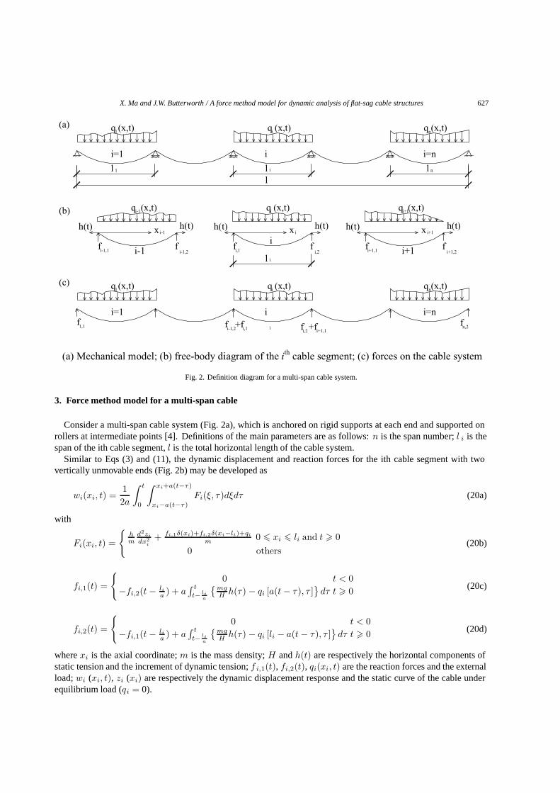
(a) Mechanical model; (b) free-body diagram of the ith cable segment; (c) forces on the cable system
Fig. 2. Definition diagram for a multi-span cable system.
3. Force method model for a multi-span cable
Consider a multi-span cable system (Fig. 2a), which is anchored on rigid supports at each end and supported onrollers at intermediate points [4]. Definitions of the main parameters are as follows: n is the span number; l i is thespan of the ith cable segment, l is the total horizontal length of the cable system.
Similar to Eqs (3) and (11), the dynamic displacement and reaction forces for the ith cable segment with twovertically unmovable ends (Fig. 2b) may be developed as
wi(xi, t) =12a
∫ t
0
∫ xi+a(t−τ)
xi−a(t−τ)
Fi(ξ, τ)dξdτ (20a)
with
Fi(xi, t) =
{hm
d2zi
dx2i
+ fi,1δ(xi)+fi,2δ(xi−li)+qi
m0 � xi � li and t � 0
0 others(20b)
fi,1(t) =
{0 t < 0
−fi,2(t− lia ) + a
∫ t
t− lia
{mgH h(τ) − qi [a(t− τ), τ ]
}dτ t � 0 (20c)
fi,2(t) =
{0 t < 0
−fi,1(t− lia ) + a
∫ t
t− lia
{mgH h(τ) − qi [li − a(t− τ), τ ]
}dτ t � 0 (20d)
where xi is the axial coordinate; m is the mass density; H and h(t) are respectively the horizontal components ofstatic tension and the increment of dynamic tension; f i,1(t), fi,2(t), qi(xi, t) are the reaction forces and the externalload; wi (xi, t), zi (xi) are respectively the dynamic displacement response and the static curve of the cable underequilibrium load (qi = 0).

628 X. Ma and J.W. Butterworth / A force method model for dynamic analysis of flat-sag cable structures
Considering all the forces acting on the whole cable system (Fig. 2c), the dynamic force method equation of (16a)may be rewritten as
d2h
dt2+ η2h =
n∑i=1
Fi(t) (21a)
with the explicit solution expressed as
h(t) =1η
∫ t
0
n∑i=1
Fi(τ) sin(ηt− ητ)dτ (21b)
where
Fi(t) =η2
r1[fi,1 + fi,2 +
∫ li
0
qi(x, t)dx], η2 =lmg2EA
leH2, r1 =
mgl
H, le
is the curve length of the whole cable, other parameters have the same meanings as the single cable system.For free-vibration analysis, assuming qi = 0 and substituting
h(t) = heiωt, fi,1(t) = fi,1eiωt, fi,2(t) = fi,2e
iωt
into Eqs (20c), (20d) and (21a), we obtain the nonlinear equation defining the natural cable frequencies, ω
ω
2− ω3
2λ2=
n∑i=1
tan(αiω
2) (22)
where
ω = ωl/a, λ2 = η2 (l/a)2 , αi = li/l.
Equation (22) is the same as the frequency equation derived by means of the displacement method [4].
4. Nonlinear model
4.1. Single-span cable model
Considering damping forces and the nonlinear effects on the dynamic response, the motion Eq. (1) may berewritten as
(H + h)∂2w
∂x2+ h
d2z
dx2+ q = m
∂2w
∂t2+ c
∂w
∂t(23)
where h and w are respectively the horizontal component of the additional dynamic tension and the dynamicdisplacement response, where the values of both take account of nonlinear effects; c is the damping coefficient.
The displacement compatibility Eq. (15) may be rewritten as
h =EA
le
[mg
H
∫ l
0
wdx +12
∫ l
0
(∂w
∂x
)2
dx
](24)
Assuming
h =N∑
k=1
εkhk (25a)
w =N∑
k=1
εkwk (25b)
X. Ma and J.W. Butterworth / A force method model for dynamic analysis of flat-sag cable structures 629
q = εq1 (25c)
c = εc (25d)
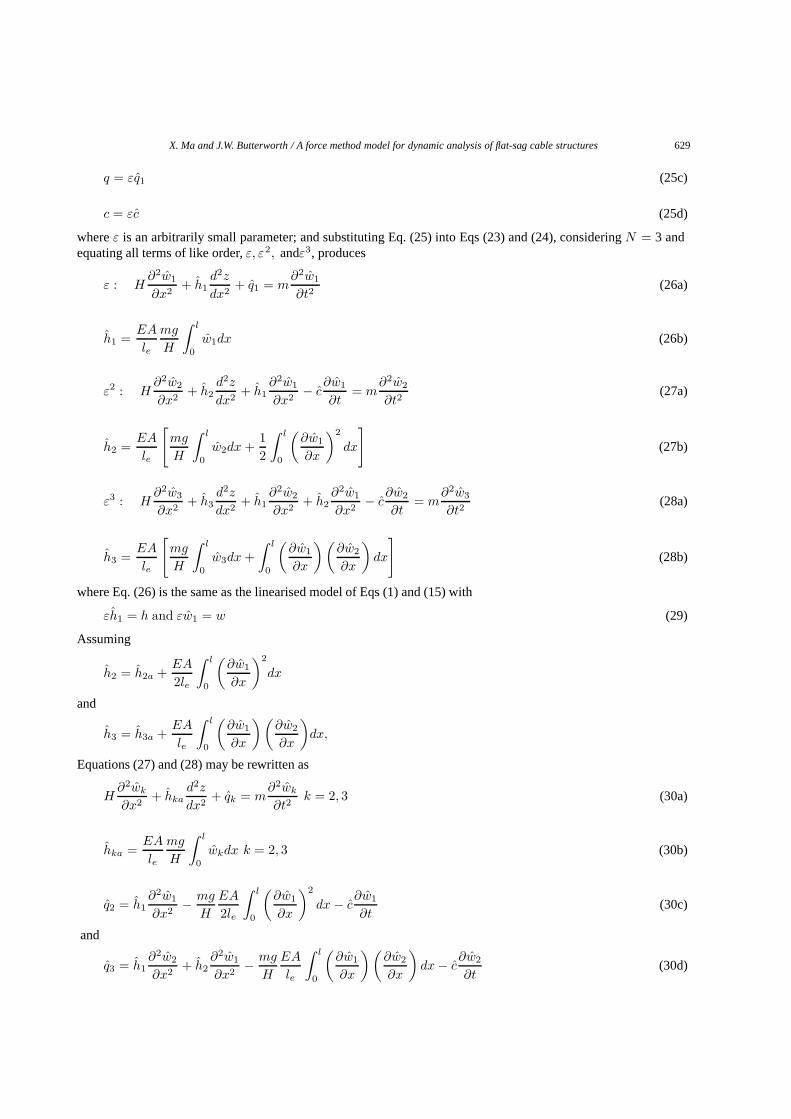
where ε is an arbitrarily small parameter; and substituting Eq. (25) into Eqs (23) and (24), considering N = 3 andequating all terms of like order, ε, ε2, andε3, produces
ε : H∂2w1
∂x2+ h1
d2z
dx2+ q1 = m
∂2w1
∂t2(26a)
h1 =EA
le
mg
H
∫ l
0
w1dx (26b)
ε2 : H∂2w2
∂x2+ h2
d2z
dx2+ h1
∂2w1
∂x2− c
∂w1
∂t= m
∂2w2
∂t2(27a)
h2 =EA
le
[mg
H
∫ l
0
w2dx +12
∫ l
0
(∂w1
∂x
)2
dx
](27b)
ε3 : H∂2w3
∂x2+ h3
d2z
dx2+ h1
∂2w2
∂x2+ h2
∂2w1
∂x2− c
∂w2
∂t= m
∂2w3
∂t2(28a)
h3 =EA
le
[mg
H
∫ l
0
w3dx +∫ l
0
(∂w1
∂x
) (∂w2
∂x
)dx
](28b)
where Eq. (26) is the same as the linearised model of Eqs (1) and (15) with
εh1 = h and εw1 = w (29)
Assuming
h2 = h2a +EA
2le
∫ l
0
(∂w1
∂x
)2
dx
and
h3 = h3a +EA
le
∫ l
0
(∂w1
∂x
) (∂w2
∂x
)dx,
Equations (27) and (28) may be rewritten as
H∂2wk
∂x2+ hka
d2z
dx2+ qk = m
∂2wk
∂t2k = 2, 3 (30a)
hka =EA
le
mg
H
∫ l
0
wkdx k = 2, 3 (30b)
q2 = h1∂2w1
∂x2− mg
H
EA
2le
∫ l
0
(∂w1
∂x
)2
dx − c∂w1
∂t(30c)
and
q3 = h1∂2w2
∂x2+ h2
∂2w1
∂x2− mg
H
EA
le
∫ l
0
(∂w1
∂x
) (∂w2
∂x
)dx− c
∂w2
∂t(30d)

630 X. Ma and J.W. Butterworth / A force method model for dynamic analysis of flat-sag cable structures
where Eqs (30a) and (30b) have similar form to Eqs (1) and (15). The force method governing equation and explicitsolution for hka are
d2hka
dt2+ η2hka = Fk(t) k = 2, 3 (31a)
hka(t) =1η
∫ t
0
Fk(τ) sin(ηt− ητ)dτ (31b)
with
Fk(t) =η2
r1
[f1,k + f2,k +
∫ l
0
qk(x, t)dx
](31c)
f1,k(t) =
{0 t < 0
−f2,k(t− la ) + a
∫ t
t− la
{mgH hka(τ) − qk [a(t− τ), τ ]
}dτ t � 0
k = 2, 3 (31d)
f2,k(t) =
{0 t < 0
−f1,k(t− la ) + a
∫ t
t− la
{mgH hka(τ) − qk [l − a(t− τ), τ ]
}dτ t � 0
k = 2, 3 (31e)
4.2. Multi-span cable model
Similar to the single-span cable model, assuming the nonlinear tension response has the same form as Eq. (25a),the external loading and nonlinear displacement response of the ith cable segment may be expressed as
qi = εqi,1 (32a)
wi =N∑
k=1
εkwi,k (32b)
where the linearised displacement response wi,1 for the ith cable segment may be calculated based on Eqs (20a) and(20b).
Thus loads due to nonlinear responses may be expressed as
qi,2 = h1∂2wi,1
∂x2i
− mg
H
EA
2le
∫ li
0
(∂wi,1
∂x
)2
dx− c∂wi,1
∂t(33a)
and
qi,3 = h1∂2wi,2
∂x2i
+ h2∂2wi,1
∂x2i
− mg
H
EA
le
∫ li
0
(∂wi,1
∂x
) (∂wi,2
∂x
)dx− c
∂wi,2
∂t(33b)
The nonlinear response hka may be calculated based on the following equation
d2hka
dt2+ η2hka =
n∑i=1
Fi,k(t) k = 2, 3 (34a)
with the explicit solution of
hka(t) =1η
∫ t
0
n∑i=1
Fi,k(τ) sin(ηt− ητ)dτ (34b)
where
X. Ma and J.W. Butterworth / A force method model for dynamic analysis of flat-sag cable structures 631
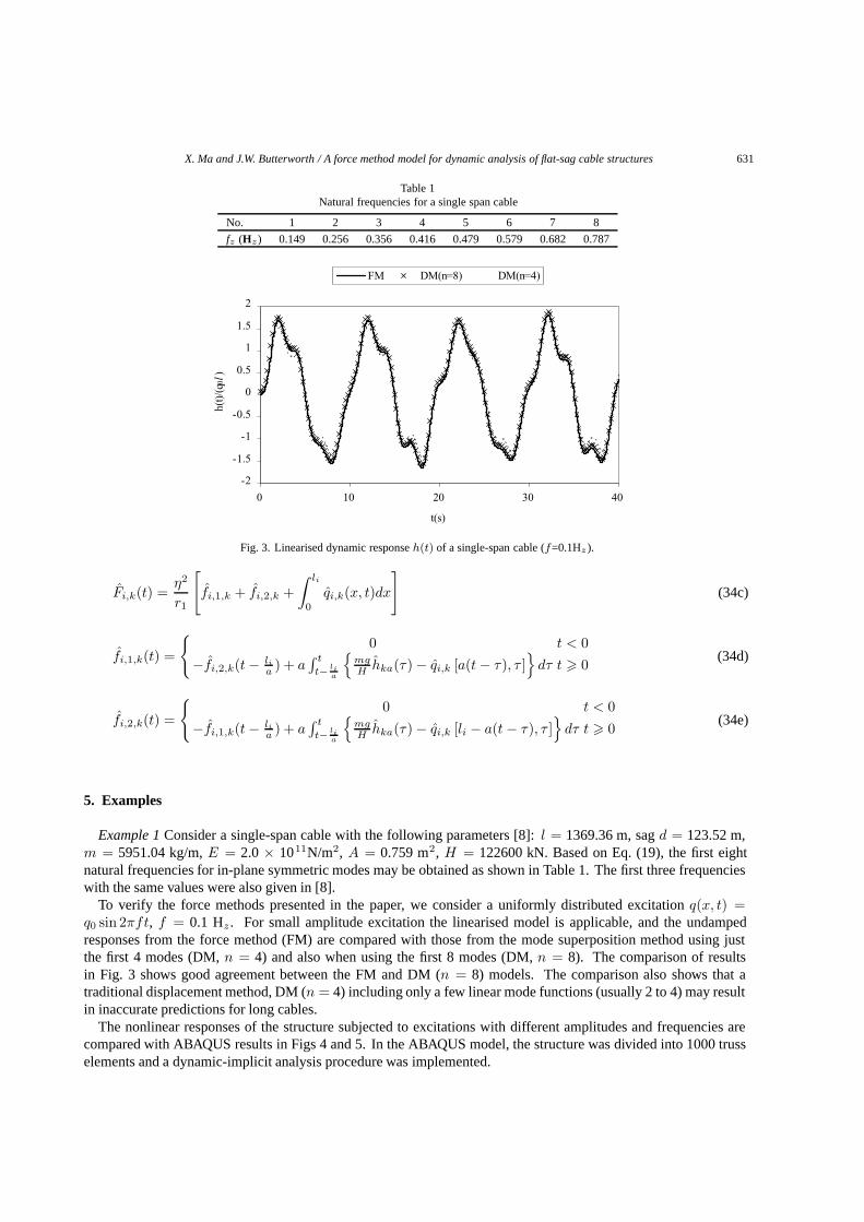
Table 1Natural frequencies for a single span cable
No. 1 2 3 4 5 6 7 8
fz (Hz) 0.149 0.256 0.356 0.416 0.479 0.579 0.682 0.787
-2
-1.5
-1
-0.5
0
0.5
1
1.5
2
0 10 20 30 40
t(s)
h(t)/
(q0l
)
FM DM(n=8) DM(n=4)
Fig. 3. Linearised dynamic response h (t) of a single-span cable (f=0.1Hz ).
Fi,k(t) =η2
r1
[fi,1,k + fi,2,k +
∫ li
0
qi,k(x, t)dx
](34c)
fi,1,k(t) =
{0 t < 0
−fi,2,k(t− lia ) + a
∫ t
t− lia
{mgH hka(τ) − qi,k [a(t− τ), τ ]
}dτ t � 0 (34d)
fi,2,k(t) =
{0 t < 0
−fi,1,k(t− lia ) + a
∫ t
t− lia
{mgH hka(τ) − qi,k [li − a(t− τ), τ ]
}dτ t � 0 (34e)
5. Examples
Example 1 Consider a single-span cable with the following parameters [8]: l = 1369.36 m, sag d = 123.52 m,m = 5951.04 kg/m, E = 2.0 × 10¹¹N/m2, A = 0.759 m2, H = 122600 kN. Based on Eq. (19), the first eightnatural frequencies for in-plane symmetric modes may be obtained as shown in Table 1. The first three frequencieswith the same values were also given in [8].
To verify the force methods presented in the paper, we consider a uniformly distributed excitation q(x, t) =q0 sin 2πft, f = 0.1 Hz . For small amplitude excitation the linearised model is applicable, and the undampedresponses from the force method (FM) are compared with those from the mode superposition method using justthe first 4 modes (DM, n = 4) and also when using the first 8 modes (DM, n = 8). The comparison of resultsin Fig. 3 shows good agreement between the FM and DM (n = 8) models. The comparison also shows that atraditional displacement method, DM (n = 4) including only a few linear mode functions (usually 2 to 4) may resultin inaccurate predictions for long cables.
The nonlinear responses of the structure subjected to excitations with different amplitudes and frequencies arecompared with ABAQUS results in Figs 4 and 5. In the ABAQUS model, the structure was divided into 1000 trusselements and a dynamic-implicit analysis procedure was implemented.
632 X. Ma and J.W. Butterworth / A force method model for dynamic analysis of flat-sag cable structures
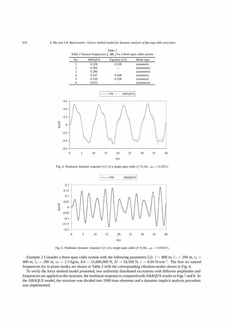
Table 2Table 2 Natural frequencies fz (Hz) for a three-span cable system
No. ABAQUS Equation (22) Mode type
1 0.228 0.228 symmetric2 0.302 – asymmetric3 0.306 – asymmetric4 0.437 0.438 symmetric5 0.529 0.538 symmetric6 0.612 – asymmetric
-0.6
-0.4
-0.2
0
0.2
0.4
0.6
0 5 10 15 20 25 30 35 40
t(s)
h(t)/
H
FM ABAQUS
Fig. 4. Nonlinear dynamic response h (t) of a single-span cable (f=0.1Hz , q0 = 0.3H/l ).
-0.2
-0.15
-0.1
-0.05
0
0.05
0.1
0.15
0.2
0 5 10 15 20 25 30 35 40
t(s)
h(t)/
H
FM ABAQUS
Fig. 5. Nonlinear dynamic response h (t) of a single-span cable (f=0.3Hz , q0 = 0.03H/l ).
Example 2 Consider a three-span cable system with the following parameters [2]: l = 800 m, l 1 = 200 m, l2 =400 m, l3 = 200 m, m = 2.3 kg/m, EA = 53,000,000 N, H = 34,500 N, c = 0.04 N-s/m 2. The first six naturalfrequencies for in-plane modes are shown in Table 2 with the corresponding vibration modes shown in Fig. 6.
To verify the force method model presented, two uniformly distributed excitations with different amplitudes andfrequencies are applied on the structure, the nonlinear response is compared with ABAQUS results in Figs 7 and 8. Inthe ABAQUS model, the structure was divided into 1000 truss elements and a dynamic-implicit analysis procedurewas implemented.
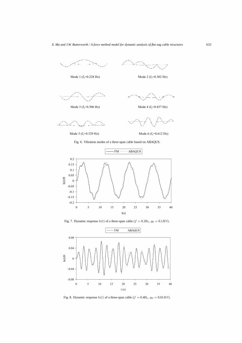
X. Ma and J.W. Butterworth / A force method model for dynamic analysis of flat-sag cable structures 633
Mode 1 (fz=0.228 Hz) Mode 2 (fz=0.302 Hz)
Mode 3 (fz=0.306 Hz) Mode 4 (fz=0.437 Hz)
Mode 5 (fz=0.529 Hz) Mode 6 (fz=0.612 Hz)
Fig. 6. Vibration modes of a three-span cable based on ABAQUS.
-0.2
-0.15
-0.1
-0.05
0
0.05
0.1
0.15
0.2
0 5 10 15 20 25 30 35 40
t(s)
h(t)
/H
FM ABAQUS
Fig. 7. Dynamic response h (t) of a three-span cable (f = 0.1Hz , q0 = 0.1H/l ).
-0.08
-0.04
0
0.04
0.08
0 5 10 15 20 25 30 35 40
t (s)
h(t)/
H
FM ABAQUS
Fig. 8. Dynamic response h (t) of a three-span cable (f = 0.4Hz , q0 = 0.01H/l ).
634 X. Ma and J.W. Butterworth / A force method model for dynamic analysis of flat-sag cable structures
-0.25-0.20-0.15-0.10-0.050.000.050.100.150.200.25
0 10 20 30 40
t (s)
grou
nd a
ccel
erat
ion
(g)
Fig. 9. Accelerogram from 1940 El Centro earthquake (vertical component).
-0.08
-0.04
0
0.04
0.08
0 5 10 15 20 25 30 35 40
t(s)
h(t)
/H
Fig. 10. Dynamic response h(t) of a three-span cable subject to vertical earthquake excitation.
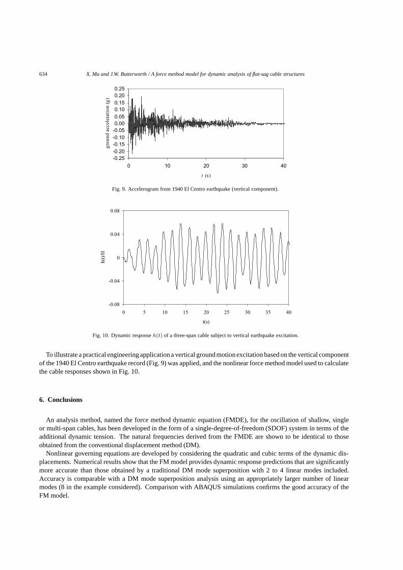
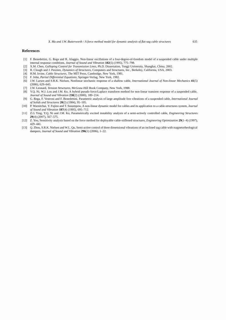
To illustrate a practical engineering application a vertical ground motion excitation based on the vertical componentof the 1940 El Centro earthquake record (Fig. 9) was applied, and the nonlinear force method model used to calculatethe cable responses shown in Fig. 10.
6. Conclusions
An analysis method, named the force method dynamic equation (FMDE), for the oscillation of shallow, singleor multi-span cables, has been developed in the form of a single-degree-of-freedom (SDOF) system in terms of theadditional dynamic tension. The natural frequencies derived from the FMDE are shown to be identical to thoseobtained from the conventional displacement method (DM).
Nonlinear governing equations are developed by considering the quadratic and cubic terms of the dynamic dis-placements. Numerical results show that the FM model provides dynamic response predictions that are significantlymore accurate than those obtained by a traditional DM mode superposition with 2 to 4 linear modes included.Accuracy is comparable with a DM mode superposition analysis using an appropriately larger number of linearmodes (8 in the example considered). Comparison with ABAQUS simulations confirms the good accuracy of theFM model.
X. Ma and J.W. Butterworth / A force method model for dynamic analysis of flat-sag cable structures 635
References
[1] F. Benedettini, G. Rega and R. Alaggio, Non-linear oscillations of a four-degree-of-freedom model of a suspended cable under multipleinternal response conditions, Journal of Sound and Vibration 182(5) (1995), 775–798.
[2] X.M. Chen, Galloping Control for Transmission Lines, Ph.D. Dissertation, Tongji University, Shanghai, China, 2002.[3] R. Clough and J. Penzien, Dynamics of Structures, Computers and Structures, Inc., Berkeley, California, USA, 2003.[4] H.M. Irvine, Cable Structures, The MIT Press, Cambridge, New York, 1981.[5] F. John, Partial Differential Equations, Springer-Verlag, New York, 1982.[6] J.W. Larsen and S.R.K. Nielsen, Nonlinear stochastic response of a shallow cable, International Journal of Non-linear Mechanics 41(5)
(2006), 629–643.[7] J.W. Leonard, Tension Structures, McGraw-Hill Book Company, New York, 1988.[8] Y.Q. Ni, W.J. Lou and J.M. Ko, A hybrid pseudo force/Laplace transform method for non-linear transient response of a suspended cable,
Journal of Sound and Vibration 238(2) (2000), 189–214.[9] G. Rega, F. Vestroni and F. Benedettini, Parametric analysis of large amplitude free vibrations of a suspended cable, International Journal
of Solids and Structures 20(2) (1984), 95–105.[10] P. Warnitchai, Y. Fujino and T. Susumpow, A non-linear dynamic model for cables and its application to a cable-structures system, Journal
of Sound and Vibration 187(4) (1995), 695–712.[11] Z.G Ying, Y.Q. Ni and J.M. Ko, Parametrically excited instability analysis of a semi-actively controlled cable, Engineering Structures
29(4) (2007), 567–575.[12] Z. You, Sensitivity analysis based on the force method for deployable cable-stiffened structures, Engineering Optimization 29(1–4) (1997),
429–441.[13] Q. Zhou, S.R.K. Nielsen and W.L. Qu, Semi-active control of three dimensional vibrations of an inclined sag cable with magnetorheological
dampers, Journal of Sound and Vibration 296(1) (2006), 1–22.

International Journal of
AerospaceEngineeringHindawi Publishing Corporationhttp://www.hindawi.com Volume 2010
RoboticsJournal of
Hindawi Publishing Corporationhttp://www.hindawi.com Volume 2014
Hindawi Publishing Corporationhttp://www.hindawi.com Volume 2014
Active and Passive Electronic Components
Control Scienceand Engineering
Journal of
Hindawi Publishing Corporationhttp://www.hindawi.com Volume 2014
International Journal of
RotatingMachinery
Hindawi Publishing Corporationhttp://www.hindawi.com Volume 2014
Hindawi Publishing Corporation http://www.hindawi.com
Journal ofEngineeringVolume 2014
Submit your manuscripts athttp://www.hindawi.com
VLSI Design
Hindawi Publishing Corporationhttp://www.hindawi.com Volume 2014
Hindawi Publishing Corporationhttp://www.hindawi.com Volume 2014
Shock and Vibration
Hindawi Publishing Corporationhttp://www.hindawi.com Volume 2014
Civil EngineeringAdvances in
Acoustics and VibrationAdvances in
Hindawi Publishing Corporationhttp://www.hindawi.com Volume 2014
Hindawi Publishing Corporationhttp://www.hindawi.com Volume 2014
Electrical and Computer Engineering
Journal of
Advances inOptoElectronics
Hindawi Publishing Corporation http://www.hindawi.com
Volume 2014
The Scientific World JournalHindawi Publishing Corporation http://www.hindawi.com Volume 2014
SensorsJournal of
Hindawi Publishing Corporationhttp://www.hindawi.com Volume 2014
Modelling & Simulation in EngineeringHindawi Publishing Corporation http://www.hindawi.com Volume 2014
Hindawi Publishing Corporationhttp://www.hindawi.com Volume 2014
Chemical EngineeringInternational Journal of Antennas and
Propagation
International Journal of
Hindawi Publishing Corporationhttp://www.hindawi.com Volume 2014
Hindawi Publishing Corporationhttp://www.hindawi.com Volume 2014
Navigation and Observation
International Journal of
Hindawi Publishing Corporationhttp://www.hindawi.com Volume 2014
DistributedSensor Networks
International Journal of