A Fixed-Wing Micro Air Vehicle with Hovering … fixed-wing micro aerial vehicle with hover flight...

AFRL-AFOSR-UK-TR-2010-0001

A Fixed-Wing Micro Air Vehicle with Hovering Capability

Jean-Marc Moschetta SUPAERO

Dept of Aerodynamics 10 Avenue Edouard Belin

Toulouse Cedex 4 France 31055

EOARD SPC 07-4010

December 2010

Final Report for 06 July 2007 to 06 July 2010

Air Force Research Laboratory Air Force Office of Scientific Research

European Office of Aerospace Research and Development Unit 4515 Box 14, APO AE 09421

Distribution Statement A: Approved for public release distribution is unlimited.

REPORT DOCUMENTATION PAGE Form Approved OMB No. 0704-0188

Public reporting burden for this collection of information is estimated to average 1 hour per response, including the time for reviewing instructions, searching existing data sources, gathering and maintaining the data needed, and completing and reviewing the collection of information. Send comments regarding this burden estimate or any other aspect of this collection of information, including suggestions for reducing the burden, to Department of Defense, Washington Headquarters Services, Directorate for Information Operations and Reports (0704-0188), 1215 Jefferson Davis Highway, Suite 1204, Arlington, VA 22202-4302. Respondents should be aware that notwithstanding any other provision of law, no person shall be subject to any penalty for failing to comply with a collection of information if it does not display a currently valid OMB control number. PLEASE DO NOT RETURN YOUR FORM TO THE ABOVE ADDRESS. 1. REPORT DATE (DD-MM-YYYY)

01-12-2010 2. REPORT TYPE

Final Report 3. DATES COVERED (From – To)

06 July 2007 - 06 July 2010

4. TITLE AND SUBTITLE

A Fixed-Wing Micro Air Vehicle with Hovering Capability

5a. CONTRACT NUMBER FA8655-07-M-4010

5b. GRANT NUMBER

5c. PROGRAM ELEMENT NUMBER

6. AUTHOR(S)

Professor Jean-Marc Moschetta

5d. PROJECT NUMBER

5d. TASK NUMBER

5e. WORK UNIT NUMBER

7. PERFORMING ORGANIZATION NAME(S) AND ADDRESS(ES)SUPAERO 10 Avenue Edouard Belin Toulouse Cedex 4 31055 France

8. PERFORMING ORGANIZATION REPORT NUMBER

SPC 07-4010

9. SPONSORING/MONITORING AGENCY NAME(S) AND ADDRESS(ES)

EOARD Unit 4515 BOX 14 APO AE 09421

10. SPONSOR/MONITOR’S ACRONYM(S)

11. SPONSOR/MONITOR’S REPORT NUMBER(S)AFRL-AFOSR-UK-TR-2010-0001

12. DISTRIBUTION/AVAILABILITY STATEMENT Approved for public release; distribution is unlimited. 13. SUPPLEMENTARY NOTES

14. ABSTRACT

The present project is the sequel of a transatlantic collaborative research project started in 2007 with the University of Arizona and the group of Dr. Sergey Shkarayev. The previous research grant was devoted to the comparative study of tilt-rotor and tilt-body configurations for Micro Aerial Vehicles (MAV). The purpose of the present study is to investigate the potential benefit of combining a fixed-wing airframe with tandem counter-rotating rotors in order to perform both fast horizontal flight phases and hovering or vertical flight phases, without resorting to a hollow shaft system as in the case of a coaxial rotor in tractor position. Also, a tandem-rotor configuration has the advantage of providing an extra degree of freedom to control the vehicle along the yaw axis. From an aerodynamic perspective, it also allow for a larger wing area within the propeller slipstream, yielding a higher aerodynamic flap efficiency and a better aerodynamic performance due to a higher aspect ratio.

15. SUBJECT TERMS EOARD, Experimental, Aerodyanamics, Micro Air Vehicle

16. SECURITY CLASSIFICATION OF: 17. LIMITATION OF ABSTRACT

UL

18, NUMBER OF PAGES

34

19a. NAME OF RESPONSIBLE PERSONBrad Thompson a. REPORT

UNCLAS b. ABSTRACT

UNCLAS c. THIS PAGE

UNCLAS 19b. TELEPHONE NUMBER (Include area code) +44 (0)1895 616163

Standard Form 298 (Rev. 8/98) Prescribed by ANSI Std. Z39-18

Final Report – research grant FA8655-07-M-4010

1

A fixed-wing micro air vehicle with hovering capabilities

Jean-Marc Moschetta1 Institut Supérieur de l’Aéronautique et de l’Espace, Toulouse, France

Abstract

The present project is the sequel of a transatlantic collaborative research project started in 2007

with the University of Arizona and the group of Dr. Sergey Shkarayev. The previous research grant was

devoted to the comparative study of tilt-rotor and tilt-body configurations for Micro Aerial Vehicles (MAV).

The purpose of the present study is to investigate the potential benefit of combining a fixed-wing

airframe with tandem counter-rotating rotors in order to perform both fast horizontal flight phases and

hovering or vertical flight phases, without resorting to a hollow shaft system as in the case of a coaxial rotor

in tractor position (Fig. 1). Also, a tandem-rotor configuration has the advantage of providing an extra degree

of freedom to control the vehicle along the yaw axis. From an aerodynamic perspective, it also allow for a

larger wing area within the propeller slipstream, yielding a higher aerodynamic flap efficiency and a better

aerodynamic performance due to a higher aspect ratio.

1 Professor of Aerodynamics, Department of Aerodynamics, Energetics and Propulsion, ISAE, BP 54032 31055 Toulouse CEDEX 4, France, [email protected]

Figure 1. The MAVion, a tandem-rotor tilt-body configuration as presented at IMAV’09

termediate report – research grant FA8655-07-M-4010

2


3

Experimental and Computational Analysis

of a Fixed-Wing VTOL MAV in Ground Effect

Chinnapat Thipyopas2, Gaurang Mehta3, and Jean-Marc Moschetta4

Department of Aerodynamics, Energetics and Propulsion, Institut Supérieur de l’Aéronautique et de l’Espace,

University of Toulouse 31400 Toulouse, France

1. INTRODUCTION

Practical MAV reconnaissance missions to be conducted in an outdoor urban environment simultaneously require the

capability of both flying fast to reach a target even in windy conditions and slowly loitering over a target in order to

capture and transmit clear images to the ground station. Because they intrinsically offer better endurance and payload

capacity than rotorcraft of equal size, fixed-wing micro air vehicles are believed to be good candidates for designing

micro air vehicles devoted to complex recognition missions. Although micro rotorcraft proved to be efficient for indoor

missions and outdoor missions with moderate wind conditions, it is believed that a fixed-wing MAV with VTOL

capacity could outperform a rotorcraft in perturbed weather conditions and still be able to perform building intrusion

and hover flight. A fixed-wing micro aerial vehicle with hover flight capability has been designed and tested. Such a

configuration is believed to be of interest for a broad range of civil and military missions because it can combine

horizontal flight for covertness and vertical flight for clear image transmission.

A first prototype of a VTOL mini-UAV called the Vertigo was successfully flown in late 2006 in manual radio-

controlled mode in order to demonstrate the capacity to safely perform transition between hover and forward flight

(Fig. 1, left). The configuration was inspired by the Convair “Pogo” and based on a coaxial propeller located in tractor

configuration in order to provide a blowing effect capable of maintaining aerodynamic efficiency of the elevons when

in hover mode. A wind tunnel campaign was carried out to extract experimental results from the Vertigo aerodynamic

characteristics. Both powered and unpowered tests were run so that the strong influence of propeller flow on the wing

could be measured. As confirmed by the measurements and by a comparison with an analytical model of the propeller

2 Research Assistant, Department of Aerodynamics, Energetics and Propulsion, [email protected]

3 Graduate student, Department of Aerodynamics, Energetics and Propulsion, [email protected]

4 Professor in Aerodynamic, Department of Aerodynamics, Energetics and Propulsion, [email protected]


4

slipstream due to McCormick [1], the alteration of the free stream through the propeller disk is responsible for enabling

steady states all along the transition flight. Therefore, some studies were derived so as to depict more accurately the

propeller wing interaction phenomena and be able to adapt the tilt body concept to MAV size.

A first experimental study of a VTOL MAV had been carried out at ISAE in cooperation with Prof. S. Shkarayev [2]

to measure the slipstream of a coaxial propulsion set using a hotwire technique. The detailed insight of the slipstream

development was compared with momentum theory and was used to properly design a 30 cm-span VTOL MAV

prototype named mini-Vertigo, which was designed and fabricated in collaboration with the University of Arizona (Fig.

1 right). Apart from transition flight, another key aspect of the design of fixed-wing VTOL MAVs is related to VTOL

and hover flight. Indeed, the MAV is simultaneously required to be sufficiently stable so as to steadily hover and

sufficiently manoeuvrable so as to counter any perturbations. In the present tractor configuration, hover flight control is

achieved by the propeller slipstream deflection using trailing edge flaps or elevons.

Figure 1. The 60-cm-UAV VertiGo (left) and the 30cm-MAV MiniVertiGo (right)

Air vehicles, both fixed wing and rotor wing type, are usually affected by ground effects as they approach an altitude

approximately equal to the aircraft wingspan or to the helicopter rotor radius. The effect increases as the vehicle

descends closer to the ground. This effect reduces an induced drag of aircraft but it can present a hazard, particularly

for inexperienced aircraft pilots. The ground effect has been thoroughly studied especially for rotorcraft. A helicopter

hovering in ground effect requires considerably less power than when it is hovering out of ground effect [3]. Ground

effect is usually presented when the rotor is close to ground at a distance lower than its diameter. Many studies had

been carried out to investigate ground effect including experimental tests [4], computational methods [5], and

visualization techniques [6]. Since there is strong interaction between airframe undersurfaces and the ground in the


5

presence of lift jets, ground effect was also considered for VTOL and STOL aircraft as well [7-8]. The study of wing in

ground effect, reported by Morris [9], shows the advantage of ground effect by an increase of 18% and 26% in lift

coefficient and lift-to-drag ratio, respectively. According to this advantage, airplanes in ground effect or ekranoplan (in

Russian, “экраноплан”), which first tested in Scandinavia just before World War II, have been developed in Russia,

USA, and China. Ground effect on a small air vehicle model was studied for a quad tilt rotor platform by Alfred

Gessow Rotorcraft Center at the University of Maryland. The experimental study of Ref. [10] found impact of ground

to airframe loads which vary from 3.6% to 15.7% of the total thrust for ground and out of ground effect, respectively.

They compared the test results with CFD results as well [11].

Fixed wing MAVs normally operate outdoors with an altitude sufficiently high so as to be able to spot ground

targets and avoid ground collision. For this reason, ground effect is not very interesting for standard outdoor MAVs.

Yet, the tail sitter VTOL MAVs developed by the University of Arizona and ISAE are designed for both indoor and

outdoor surveillance missions. They are designed for autonomous vertical take-off and landing and should be capable

of hovering over a horizontal target. Ground may indeed introduce some perturbations during vertical take-off and

landing or when hovering over a horizontal plane such as a table. Therefore, a dedicated experimental bench has been

used to measure the hover flight performances, both in terms of propulsion and aerodynamic efficiency. Ground and

wall effects have been especially analyzed in view of predicting the vehicle behavior in take-off and landing phases. To

investigate ground effect on a MAV with a very small weight and very low aerodynamic force, the experiment is

carefully carried out on a very high performance force balance.

2. A FIXED-WING TANDEM-MOTOR MAV: MAVion

The coaxial concept is well adapted for mini size electric motor by using a hollow shaft. Many flying objects now use

this system, in particular RC-commercial coaxial helicopters, due to its benefit of torque elimination without tail rotor.

Tail-sitter fixed-wing VTOL MAVs also require this advantage, especially for the VTOL and hovering phase.

However, this mechanism is difficult for miniature motor sizes. A coaxial system has been realized for a micro size

flying robot as seen in the Fig.1-right The MiniVertiGo used two big motors of 20g-weight-each which gives a thrust of

500g (5N). This is high compared with vehicle’s mass of 243 grams. The coaxial concept is difficult to realize for the

smaller size of flying objects envisioned in future development. The propulsive-wing interaction study of Thipyopas

[12] also mentioned an improvement of wing aerodynamic performance by using side-by-side tandem tractor propellers

rotating so as to counter wingtip vortex. Accordingly, the new design of a VTOL MAV, called MAVion, is conducted

by a group of students from ISAE. Initially, MAVion consists of a simple rectangular wing, side-by-side tandem tractor

propulsion, one vertical stabilizer, and a main fuselage for integration of the electronics. Finally, wing planform has


6

been modified by applying taper to reduce the maximum size and to improve wing aerodynamic efficiency. According

to the study of Ref. 2, the propellers are placed 65mm-ahead the wing leading edge in order to gain the maximum

propwash speed on the main wing. The final MAVion version is shown in Fig. 2-left. The wing has a root chord of

180mm, tip chord of 100mm, and span of 300mm. Two 3-blade GWS 5030 contra-rotating propellers are installed at

80mm-span from the central. Two control surfaces are placed on the trailing edge for both pitch and roll control. This

MAV is specially designed to perform both forward flight and hovering. The MAVion has already demonstrated it

horizontal forward flight performance by taking first place at the IMAV09 competition.

Figure 2. The MAVion Tandem-Motor VTOL MAV

Hovering in ground effect is another key issue of this VTOL MAV. Although the ground height-to-propeller ratio of

the MAVion is markedly greater than propeller size when landing, the control surfaces are very close to the ground. The

aerodynamic characteristics of the MAVion may be influenced by the ground when it hovers near to ground or other

horizontal planes (Fig. 2-right). Also, the size of horizontal ground surface may be comparable to the size of the

rotor/propeller in situations such as landing on a table. The aerodynamics in partial ground effect could be different.

Therefore, ground effect is only studied for comparatively large surfaces in this report.

3. CONFIGURATION DESIGN AND COMPUTATIONAL APPROACH

3.1 Geometry and CAD file definition

In order to develop a 3D geometry of the aircraft, a CAD design method developed by Dassault Aviation, CATIA

V5, has been used. Figure 3 describes the overall sketching and development of the body using several tools like

sweeping, revolve and scaling for desired output. After creating a wing and fuselage body we need to create a filleting


7

along the wing-fuselage junction for better aerodynamics performance. The MAVion geometry consists of a fuselage,

thick wings attached to it, motor mounting and a pair of elevons.

Figure 3. Basic techniques to design in CATIA

After creating all basic parts which consist of wing, body, fin, propeller, motor mounting system, all parts are

assembled using the assembly work batch. Figure 4 illustrates the final model of MAVion after assembling all parts.

Figure 4. Final assembled model of MAVion

Sketch

Fuselage and wing body

Control surface

Motor mount


8

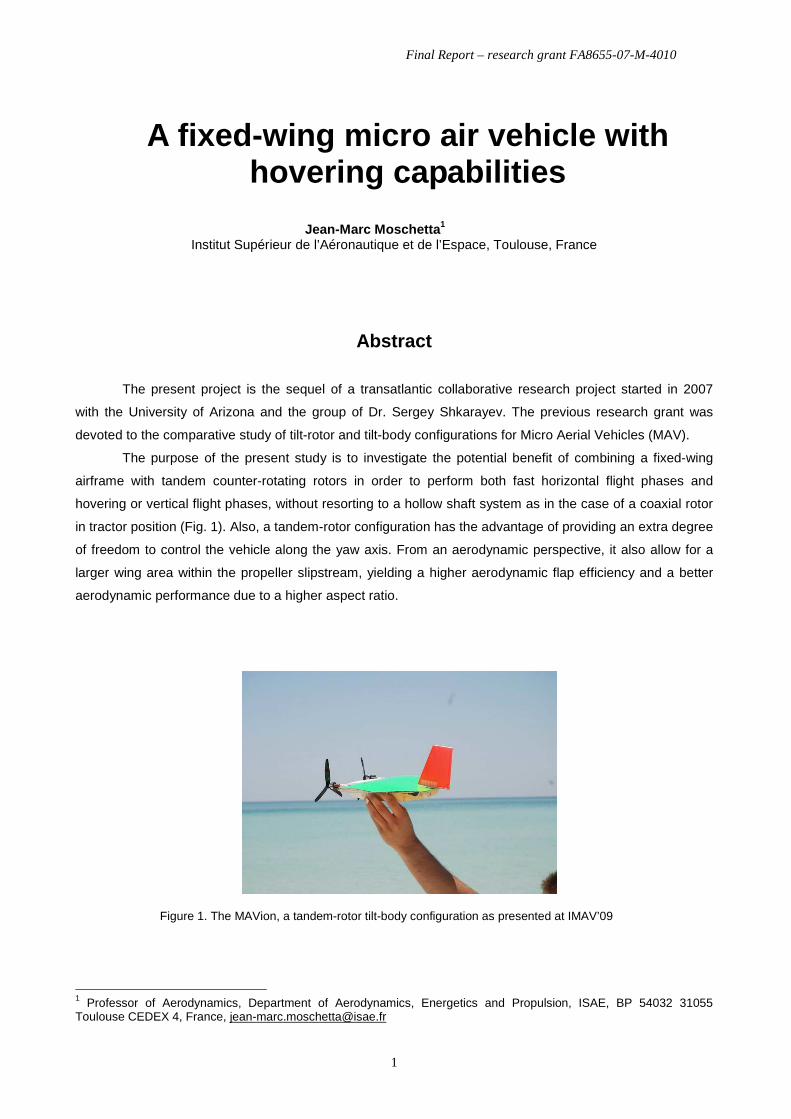
Figure 5. Engineering drawing of MAVion

3.2 A 3D unstructured grid generation

In view of generating the grid around the body, the first step is to create the appropriate geometry of the body as

described above. Since for the moment only the longitudinal problem is considered and the geometry is symmetrical,

only half of it has been meshed. Also the propeller disk has been modeled following the disk actuator theory. Namely

Philips’ model has been applied so that only pressure difference and velocity distribution is given along the disk

surface as boundary conditions. Figure 6 illustrates the computational domain which extends 1.5 wing root chord

upstream, approximately 5 chords downstream. In the spanwise direction, the computational domain extends

approximately 2.5 wing half span.

Figure 6. Computational domain around the geometry


9

In the present project the choice was to first generate an unstructured grid because only inviscid effects are considered

as a first step. Generating an unstructured 3D grid is also less time consuming and allow for a reasonably good pressure

field computation. In a second phase of the project, boundary layer effects will be accounted for through the addition of

prismatic cells along the body surface.

Figure 7 and 8 show two side views of the resulting grid. Further grids are currently under consideration.

Figure 7. General Meshing Methodology

Figure. 8 Close view near surface body

3.3 Disk actuator model

In general, the classical momentum theory is used to calculate the performance of propeller blades following a

streamtube analysis as illustrated in Figure 9. The stream tube is assumed to extend from a plane infinitely far upstream

from the propeller disk to a plane infinitely far downstream. All of the fluid that enters this stream tube on the far

upstream side must pass through the propeller disk and exit the stream tube on the far down stream side.


10

Figure. 9 Stream tube notation

In addition to the foundation hypothesis of stream tube shown in Fig. 1, classical propeller momentum theory imposes

five simplifying approximations. The flow is assumed to be 1) inviscid and 2) incompressible; 3) all rotation of the

fluid within the stream tube is neglected; and both 4) the velocity and 5) the static pressure are assumed uniform over

each cross section of the stream tube. With these approximations the induced velocity Vi is expressed as a function of

the free stream velocity V∞ and the thrust T. In dimensionless form the result is

Where,

and are the usual thrust coefficient and advance ratio

respectively. Here, ω is used to represent the propeller angular velocity, dp is the propeller diameter, and ρ is the fluid

density. From the same analysis the propulsive efficiency for the propeller is found to be

Where Q is the torque required to drive the propeller and ηi is propulsive efficiency. Philips’ theory [13] describes

that swirl of propeller wake is very important property of propeller modeling. Moreover, here conventional velocities

are included which simulate the propeller induced slipstream effect. After applying Bernoulli hypothesis, momentum

formulations and many algebraic manipulations, Phillips established a relation between the thrust force and the velocity

at propeller inlet plane:

Or in terms of average pressure difference:


11

Where,

T = Thrust force,

V∞ = Free stream velocity,

V∞ + Vi = Velocity at propeller inlet plane,

ω = Rotational speed of propeller

Rp = Propeller Radius

V i = n x X D swirl X n propeller

Where , n propeller = Propeller Rotational speed.

4. A VALIDATION OF NEW HIGH PERFORMANCE MICRO-STING-FORCE BALANCE

The challenge of the complex aerodynamics of Micro Air Vehicles and Nano Air Vehicles is presently attractive to

aeronautical engineers. Forces and moments of these flying robots are very small and difficult to measure by a

traditional force balance. To optimize the aerodynamic performance of a MAV, the study of its aerodynamics requires

very high accuracy research facilities. Therefore, ISAE-Supaero campus had a new high performance micro sting

balance for MAV research fabricated by the Institut Aerotechnique. The characteristics and validation test of this new

balance are detailed in this section.

4.1 Characteristics of Micro Sting-Balance (MicroB)

The 5 component Micro Sting Balance (MicroB) has a 10N capacity in the normal force Z, and the lateral force Y, and

a 0.5m.N moment capacity in roll L, pitch M, and yaw moment N. It is made of high strength 35NCD16 alloy steel.

The MicroB balance has a maximum length of 90mm and a maximum diameter of 8mm as illustrated in Fig. 10. The


12

centre of measurement is located at the mechanical center of the balance which means it is placed at 45mm from the

end of the balance. The balance is equipped with 5 strain gauges of K-alloy type which support a wide temperature

range. The strain gauges were attached with M600 hot adhesive. The Z, M, Y, and N components are equipped with

type WK 06 125PC 350 linear strain gauges while the other component (L) is equipped with a type SK 06 062TH 350

torque strain gauge. Finally, all strain gauges are covered by M coat D, a protective moisture barrier. The strain gauges

can be supplied by a maximum tension of 10-Volts although the supplied nominal electric tension is recommended at 4

Volts for all components where the strain gauge is auto-compensated for temperature.

Figure 10. High Performance Micro Sting Balance MicroB

4.2 Hardware and Installation of MicroB Validation Test at ISAE

4.2.1 Electronic Hardware

The balance is supplied by 4Volts DC generated by an ANS E 300 power supply/conditioner. The electric tension

supplied to the balance is controlled by a high accuracy Volt meter with a precision of 0.001V. A gain of 1000 and a

filter at 1 Hz are applied to the output signal from the balance. The treated signals are then sent to the USB-6218 M

Series data acquisition card National Instruments (NI). The analog voltage range of this card is normally set at -10 to

+10V; however, it is adjusted to the range of -1 to +1V in order to gain highest digital resolution.

4.2.2 Mechanical Setup

The balance is carefully attached to a rigid support and is calibrated by a digital angle instrument (Schaevitz AngleStar

Digital Protractor Model DP-60) which has an error less than 1% and a resolution of 0.1°. Institut Aerotechnique

calibrated the MicroB by applied force in only one direction, therefore coupling effects between the Y and Z directions

were not tested. During an actual aerodynamic measurement, however, all three forces and three moments are applied.

A validation test was performed to determine the extent of coupling between the X, Y, and Z components. The overall

validation set up is presented in Fig. 11 with all forces and moments applied. In Fig. 11c, the force in the X direction is

applied by a mass of 200g presented on the left side of photo.


13

(a) (b) (c)

Figure 11. Validation Test Set Up at ISAE a) Balance with the mass support and the cylinder beam for applying lateral force

b) Test set up with 200grams mass apply at the centre of balance

c) Coupling of axial, normal and lateral force on the balance

4.3 Validation Test Description

The measurement error (i.e. the closeness of the measurement to the true value) which can be written in the form of Eq.

(1), is clearly determined if the true value is known. Accuracy is inversely related to bias. In the experiment, the true

value is frequently unknown and it is therefore impossible to determine the accuracy. It is, however, possible to

determine the accuracy or measurement error using a standard reference mass. To verify the capacity and to identify

the error or accuracy of the MicroB balance, the reference masses are measured by a highly accurate Sartorius balance

which has a maximum capacity of 2kg and an accuracy of 10-4 grams or approximately 10-5 N.

refm−=ε (1)

Data is collected through the Labview interface at 1 kHz. Mean and standard deviation are calculated from 1000

data samples for each measurement. 110 random force / moment measurements are performed in this validation test.

The maximum and minimum load applied ranges from 1g to 400g and 1g.cm to 2000g.cm for forces and moments

respectively. For the first 60 cases, a single load is applied and zero acquisition is performed before the next test. In

each case after zero acquisition is done, the test is then followed by 25 measurements to study repeatability of the

system. The effect of applying force in the axial direction is also evaluated for test numbers 51 to 60 and test numbers

91-110 by putting 200g of mass in the X direction. For test numbers 61-100, validation is conducted to study the effect

when applying continue force which means that no zero acquisition is performed for the next load. The mass is

suddenly added to the system and then a measurement is performed. 25 measurements are conducted for each applied

load. Increased load and decreased load cases are conducted to define the hysteresis of system. All tests are detailed in

table 1.

200g

Lateral Force


14

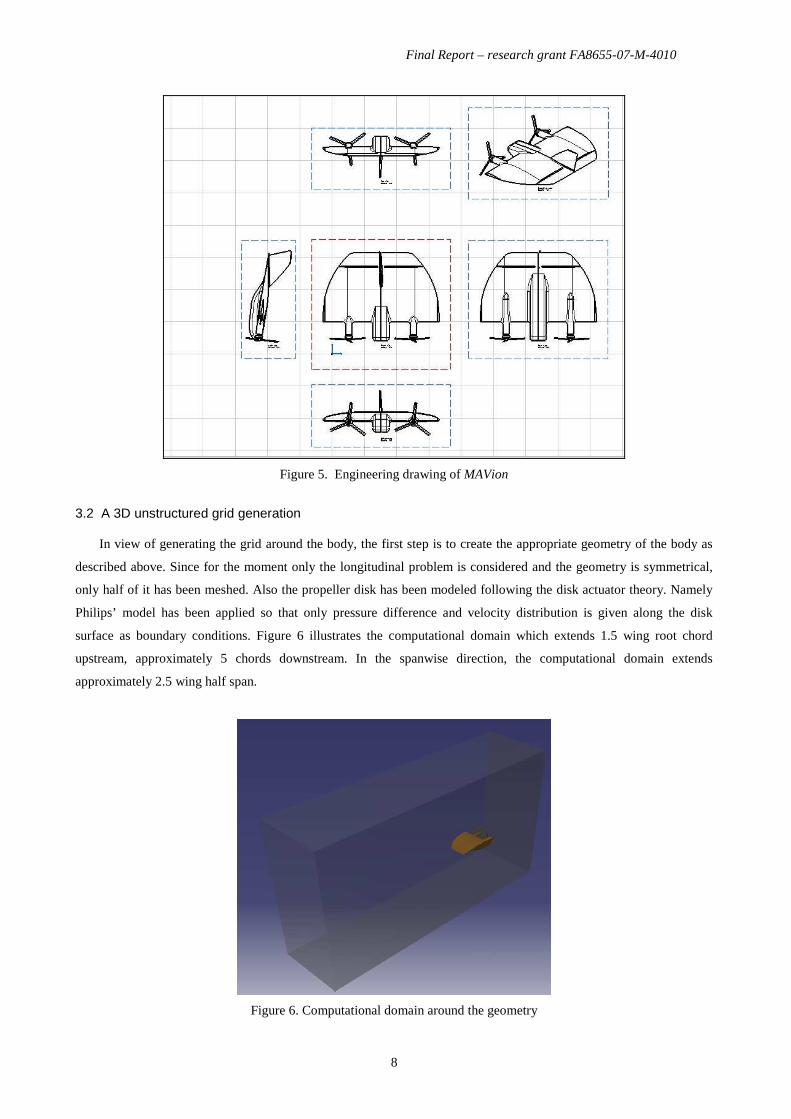
Table 1 Summary of the Validation Study

Test no. Case Description

1-50 Single Load Case Zero acquisition is performed every time before apply load (Y,

Z, L, M, and N)

51-60 Single Load and Force in X

Direction is applied Same as Test no.1-50 but force 200g in X direction is applied

61-70 1 Way Continuous Load Zero acquisition is performed before continuously apply load in

one way (increasing or decreasing)

71-90 2 Way Continuous Load Zero acquisition is performed before continuously apply load in

two ways (increasing and then decreasing)

91-100 2 Way Continuous Load and Force in

X Direction is applied Same as Test no.71-90 but force 200g in X direction is applied

101-110 Motor Influence Test Turn on power supply and run brushless motors close to the

balance

4.4 Validation Test Result

4.4.1 Quantization Error

This parameter is defined by the performance of the acquisition card (number of bits) and by the input voltage range.

This error is due either to rounding or truncation. For an ideal analog-to-digital convertor where the quantization error

is uniformly distributed between -1/2 LSB (Least Significant Bit) and +1/2 LSB, the quantization error of the system

should be equal to Vq µε 26.152

)1(121

16=−−×= so the system resolution should be as small as 0.045g-force and

0.1g.cm-moment if all the equipment is functioning ideally. However there are also other influences in practical use

such as high jumping of voltage between each channel. National Instrument gives an accuracy range of 2.69mV and

0.088mV for voltage input range of -10 to +10V and for -200 to +200mV respectively. The accuracy range for the

voltage input range of -1 to +1V used in this study then should not be better than approximately 0.25mV or about 0.7g

(7E-3N) for the forces and about 1.6g.cm (1.6E-4N.m) for the moments.

4.4.2 Precision

Measurement precision is determined by repeating acquisition several times. The standard deviation is applied into Eq.

(2) with 95% confidence interval (student t factor = 1.96) and the average precision of each component is detailed in

Table 2. The precision presented in the Table is based on 500 total measurements (1000 samples for each

measurement).

σN

tU = (2)


15

Table 2 Precision of acquisition and measurement

Component: Y (N) Z (N) L (N.m) M (N.m) N (N.m)

Acquisition Precision (1000

acquisitions)

1.83E-4 2.11E-4 6.85E-6 4.42E-6 5.35E-6

Measurement Precision 2.95E-3 3.41E-3 1.11E-4 7.139E-5 8.632E-5

Acquisition precision, given in the second line of the table, represents the scatter of 1000 samples when one

measurement is performed. It is high but still less than about 2E-4 N-force (2E-5 grams) and 7E-6 N.m-moment (7E-5

gram.cm). This precision is better than the quantization error of the acquisition card. This measurement is done for a

very short period (1sec) so this acquisition system precision does not take into account an undetermined random noise.

4.4.3 Non-Repeatability of measurement

The standard deviation of numerous measurements of an identical load can represent the non-repeatability of the

experimental system. This characteristic also presents the scatter of numerous measurements which can represent the

measurement precision. As the validation is conducted by 25 measurements for each applied load, non-repeatability or

measurement precision of the system can be determined by these repeated measurements. It is found that the overall

system has a non-repeatability corresponding to 0.0029N, 0.0034N, 1.1E-4N.m, 7.1E-5N.m, and 8.6E-5N.m as

presented in Table 2.

4.4.4 Hysteresis

Hysteresis occurs when the system is repeatedly wiggled back and forth. One can ask the question, “If the balance is

pushed, it will yield and when it is released, does it spring back completely?” Hysteresis is usually determined by

appling the force and then releasing. In this test, the mass and moment are applied step by step from zero to maximum

of 0.98N, 2.94N, 0.049N.m, 0.049N.m, and 0.024N.m, for Y, Z, L, M, and N respectively, and then the masses are

released. The test was done by using 2 examples. 95% confidence interval and student t distribution are applied again.

The most significant hysteresis effects are found at zero and are equal to 0.00889N, 0.0088N, 0.000136N.m,

0.000224N.m, and 0.000165N.m, for Y, Z, L, M, and N respectively.

4.4.5 Error of MicroB and System


16

The error of the new balance can be determined and it is shown in Table 3. The error of the balance is approximately

equal to 1g (1E-2N) and 10g.cm (1E-3N.m) for forces and moments respectively. There is no significant difference of

determined error between single-load test and continuous-load test.

Table 3 Error of balance and system

Y (N) Z (N) L (N.m) M (N.m) N (N.m)

All 110 case 0.0100 0.0072 0.00088 0.00038 0.00137

Single 0.0125 0.0087 0.00124 0.00065 0.00115

Continuous 0.0090 0.0022 0.00071 0.00017 0.00072

X 0.0077 0.0056 0.00213 0.00033 0.00143

Motor 0.0082 0.0033 0.00082 7.9E-5 0.00098

Continuous + X 0.0075 0.0118 0.00050 0.00014 0.00328

4.4.6 Effect of Axial Force

To study the effect of axial force on the balance, a 200 gram mass is applied in the X direction as shown in Fig.11c.

The measurement error is analyzed following the same method. Totally, 20 tests of different single and continuous

applied load cases are carried out. The investigation presents no effect of force in X direction on the error of all

components. The error of all components from this test is not bigger than that obtained by the test without force in the

X direction.

4.4.7 Effect of Running Brushless Motors

10 single load tests are done while two brushless motors are running in order to indentify the effect of power supply

and magnetic field induced by the motor. The distance between the motor and the balance is randomly varied between

30 and 80 cm. The motor is powered by 11Volts DC generated by a N5766A DC power supply from Agilent

Technologies. The motors run at 80% of the PWM signal and roughly correspond to a total of 3.5Amps. The error and

standard deviation between motor running and the motor not running are compared. However, no significant effect

from the power supply and motor are observed.

4.4.8 Calibration Matrix Error

This error normally depends on the magnitude of the applied mass, generally increasing as more loads are applied. This

is due to the calibration matrix error. Figure 12 presents the balance error found in this study and it is plotted with the


17

absolute value of input load. It clearly shows that the error is progressively increasing with the input load. It can be

mentioned that the error at small load is close to zero is mainly due to zeroing the acquisition error and the capacity of

the balance itself. A linear relation of % error can be noticed between the zero and maximum load. The error of the

system is then detailed in Table 4. The 2nd and 5th columns mention the number of data which used for determine the

error at zero and at maximum load respectively.

0

0.005

0.01

0.015

0.02

0.025

0.03

0.035

0.04

0.045

0.05

0 1 2 3 4 5

Input (N)

Err

or (

N)

Error Y

Error Z

0

0.001

0.002

0.003

0.004

0.005

0.006

0.007

0 0.05 0.1 0.15 0.2

Input (N.m)

Err

or (

N.m

)

Error L

Error M

Error N

Figure 12. Distribution of error as a function of the input load

Table 4 Error function of new balance

Number of data (Zero / Max)

Error Function Number of data (Zero / Max)

Error Function

X (N) - Not available L (N.m) 35 / 8 0.000951+0.008008L Y (N) 32 / 6 0.00714+0.008127Y M (N.m) 32 / 8 0.000297+0.000129M Z (N) 17 / 6 0.00722+0.002020Z N (N.m) 49 / 5 0.000801+0.039101N

5. IN AND OUT OF GROUND EFFECT TEST OF MAVion MAV

The measurements of ground effect on the MAVion configuration have been done using the MicroB. The description of

the experimental setup and the results are detailed in this section.

5.1 Approach


18

A dedicated experimental test bench has been used to study ground effects as well as flight control efficiency both in

ground effect (IGE) and out of ground effect (OGE). The test bench mainly consists of a newly acquired 5-component

MicroB which had been validated in the previous section. The complete powered aircraft was attached to the balance so

that all aerodynamic forces and moments, with the exception of the side force, were measured by this accurate sting

balance. In hover, both IGE and OGE tests are performed by varying tail-to-ground vertical distance (H).

The model consists of two propulsion sets, a main wing, a fuselage, two horizontal tails and two vertical tails as

presented in Fig.13. Each propulsion set consists of LRK 13-6-11Y -GoldLine brushless motors and a pair of 3-blade

GWS-5030 contra rotating propellers. In order to correctly observe interaction between the motor thrust and the

aerodynamic forces on the airframe, motors are fixed to the propulsive force load cell (PLC) via a motor support and

then the PLC is supported inside the main wing on the left and right side as indicated in Fig. 13-left. The MAV wing

and fuselage are made of light aluminum instead of polystyrene to improve structure and precision when fixed with the

balances. The flatplate wing thickness is equal to 11mm which is thick enough for holding the 7mm-thick PLC. The

ground effect test set up is presented in Fig.13-right. The MAV model is supported through the 8mm-diameter sting

force balance by an adjustable vertical transverse mounting system. The model altitude (H) which is measured

vertically from the trailing edge to the ground is controlled by a high precision stepping motor. The error of the altitude

adjustment is less than 0.1mm. The tests are performed with an altitude H that varies from 0 to 600mm. At this

maximum altitude, the propeller disc is about 6 times the propeller diameter above the ground so that it is expected to

induce no ground effect. Two control surfaces, chord length of 40mm, are adjusted up to 30deg in order to investigate

their efficiency in and out of ground effect at different altitudes H as well. Additional parameters including

temperature, ambient pressure, motor speed, electric consumption, and electric voltage were also recorded. The errors

and standard deviations of measurement data are estimated. The uncertainties of results are calculated according to the

small-sample method of Ref. 14.


19

Figure 13. VTOL MAV model (left) and ground effect experimental setup (right).

5.2 Results and Discussions

5.2.1 Characteristics of Propulsion (OGE)

The test of single motor OGE has been conducted by placing the propeller disc at a height of 800mm- from the ground.

The maximum thrust obtained by this propulsion system is equal to 1.59N at a motor speed of 12,000 RPM. The result

is presented in Fig. 14. The motor speed is controlled with an uncertainty less than ±75 RPM which is approximately

equal to the error of the speed sensor for each measurement. The thrust coefficient ))(/( 2 ARTCT ωρ= of the

propulsion system approximately equals 0.016. Because motor torque is not measured, only electrical input (P=IV) can

be determined. Therefore, power loading )/( PTPL= is presented in Fig. 14-bottom, instead of Figure of Merit

(FoM). The propulsion system has a better efficiency when it rotates at a lower speed. It can be noticed that error bars

at low speed are larger than error bars at high speeds because of the relative error in speed measurement.


20

Static Thrust & Thrust coefficient of Single Motor-Propeller

CT

Thrust

0

0,02

0,04

0,06

0,08

0,1

6000 7000 8000 9000 10000 11000 12000

RPM

CT

0

0,3

0,6

0,9

1,2

1,5

Thr

ust

(N)

Power Loading of Single Motor-Propeller

0,02

0,025

0,03

0,035

0,04

0,045

0,05

0,055

6000 7000 8000 9000 10000 11000 12000

RPM

Pow

er L

oadi

ng [N

/W]

Figure 14. Characteristics of single motor-propeller OGE

However, at the maximum speed of 12,000 RPM, the motor and speed controller are subject to high electric

currents, and it is not safe to operate at maximum throttle for long periods of time. In addition, the required thrust of

120 grams, which corresponds to the expected MAV weight of 240 grams, is supplied by at motor speed between

9,000-10,000 RPM. Therefore, the measurement in this ground effect study has been done at speeds ranging from

6,500-11,000 RPM.

5.2.2 Ground Effect on Propulsion

A ground effect test is then conducted by gradually increasing the tail-to-ground distance for H = 0, 25, 75, 150, 250,

400 and 600 mm. The first result in Fig. 15-top shows the variation of motor speed during the ground effect test. It

exhibits that the speed is quasi constant over all the test range.


21

Evolution of motor Speed

6000

7000

8000

9000

10000

11000

12000

0 100 200 300 400 500 600 700

Height (mm)

Spe

ed (

RP

M)

Propulsive Thrust of VTOL MAV

0,6

1

1,4

1,8

2,2

2,6

3

0 100 200 300 400 500 600 700Height (mm)

Thr

ust

(N)

6500 RPM 8000 RPM 9000 RPM 10000 RPM 11000 RPM

Figure 15. Evolution of propeller speed and propulsive thrust during GE tests.

Total thrust of two propulsion sets is illustrated in Fig. 15-bottom. The propulsion set roughly gives thrust of 1, 1.5,

1.9, 2.3, and 2.8N for motor speeds of 6 500, 8 000, 9 000, 10 000, and 11 000 respectively. Hence, ground effect on

the MAV thrust is not clearly presented by the above figures. Ground has no effect on thrust of motor-propeller at low

speed of 6 500 to 9 000 RPM. At the maximum test speed, the thrust at H = 0 has approximately only 2% greater then

the thrust at OGE. However, this result may due to the small increment of motor speed as seen in Fig.15-top. The

motor thrust coefficient is also calculated as a function of motor speed and height, showing no significant effect. The

results in thrust coefficients are scattered around a value of 0.016. A maximum calculated CT of 0.0165 is found at a

maximum speed of 11,000 RPM when the MAV is placed on the ground. However, this change of CT is very small if

compared with the error of the results.

In order to investigate the influence of ground effect on the motor-propeller efficiency, the power loading (PL) has

been calculated. Figure 16 indicates a small ground effect on PL of the VTOL MAV, particularly at high speeds of

10,000 and 11,000 RPM where an improvement in PL is evaluated around 3.4 and 5.8%, respectively. These


22

increments of PL result from both a small increase in thrust and a small reduction of electric power input when the

MAV gets closer to the ground. At higher motor speeds, the electric power decreases by about 2 Watts from 78 to 76

Watts for ground distances of 600 and 0 mm, respectively. In this case, the presence of the ground may introduce some

influence on the propeller performance through tip loss reduction as observed in large rotors. Nevertheless, the

influence of ground to the power loading examined in this investigation is not significant.

Power Loading of Propulsive System

0,03

0,035

0,04

0,045

0,05

0,055

0,06

0 100 200 300 400 500 600 700Height (mm)

Pow

er L

oadi

ng: P

L (N

/W) 6500 RPM 8000 RPM 9000 RPM

10000 RPM 11000 RPM

Figure 16. Evolution of power loading of propulsion set in GE test

5.2.2 Ground Effect on Clean Wing Characteristics

Ground effect on the clean-wing aerodynamic characteristics is also determined, especially for the download force of

MAV induced by propwash flow. The drag or download force induced by propulsive flow (Dp) is then calculated by

the total vertical force (Ftotal) measured by the sting balance and thrust (T) measured by propulsive force sensors.

In order to calculate aerodynamic coefficients, momentum theory is applied to determine the average reference

velocity (Vp) induced by the propellers. Furthermore, since propulsive induced flow does not blow all wing surfaces,

only the wing surface located in the propeller slipstream is considered in the calculation. The induced velocity and drag

coefficient of VTOL MAV calculated by Eq. 3 and 4 are illustrated in Fig. 17. The subscript p in these equations refers

to the propeller. Thrust of motor 1 and motor 2 (right and left side) is denoted by T1 and T2, respectively.

ATTVp ρ/)( 21 += (3)

)21

/()]([ 221 pptotalD SVTTFC

pρ+−= (4)


23

Because propeller thrust as a function of the ground distance is almost constant, the calculated induced velocity is

also constant as plotted in Fig.17-top. However, the calculated drag coefficient denoted by lower symbols in the same

figure significantly varies with ground distance, particularly when the MAV is approaching the ground. The drag

coefficient induced by the propeller, CDp , reduces from about 0.058 when it is out of GE to about 0.038 when it lands

on the ground. It is remarkable that the drag coefficient induced by the propellers remains almost constant for a given

altitude and does not dramatically vary with the motor speed or propulsive induced flow. The small variation of the

results may therefore be a consequence of Reynolds effects and measurement errors.

To identify a drawback of the MAVion tractor configuration, the drag force to total vertical force ratio is illustrated

in Fig. 17-bottom. The percentage of download force varies from 9.5% to 6% for the case of OGE and IGE,

respectively. This means that there is a 10% additional drag penalty due to the blowing effect in hover flight for this

7%-thickness symmetrical-airfoil wing MAV model. Since the parasite drag is a combination of pressure drag and skin

friction drag, this download–to-total force ratio should vary with airfoil types and thickness. From the experiment, it

turns out that hovering VTOL MAV in ground effect uses less energy than when hovering out of ground effect due to

the reduction of drag force. However, the ground effect may introduce other disadvantages to the vehicle such as a

reduced efficiency of control surfaces which will be investigated and presented in the next section.

Determined Induced Speed and Wing Drag Coefficient

CD

6500 RPM

8000 RPM

9000 RPM

10000 RPM

11000 RPM

0

0,02

0,04

0,06

0,08

0,1

0,12

0,14

0,16

0 100 200 300 400 500 600 700Height (mm)

CD

p

0

2

4

6

8

10

12

14

16

Indu

ced

Vel

ocity

; Vp

(m/s

)


24

Down Load Force to Total Force Ratio

4

5

6

7

8

9

10

11

12

0 100 200 300 400 500 600 700Height (mm)

% D

p/F

tota

l

6500 RPM 8000 RPM9000 RPM 10000 RPM11000 RPM

Figure 17. Ground effect on download or drag of VTOL MAV

A lift force induced by propwash flow is observed in this test as well. The lift force (lateral force) randomly varies

between 0.02 to 0.12N (around 2 to 12g.) for motor speeds between 6,500 to 11,000 RPM, respectively. At constant

motor speed, there is no important ground effect on the VTOL MAV lift force. Figure 18-top presents a lift coefficient

normalized by the propulsive induced velocity as in Eq. 5. An influence of ground and of rotational speed is hardly

noticeable. The uncertainty of result remains high compared with the scatted data for CLp. The ground effect on lift for

small MAV can not be clearly evaluated by this test. It can only be mentioned that, globally, CLp is presented in this

configuration and it is approximately equal to 0.02 when normalized by the propulsive induced velocity calculated by

the momentum theory.

)21

/( 2ppL SVLC

pρ= (5)

Lift Coefficient

-0,04

0

0,04

0,08

0 100 200 300 400 500 600 700

Height (mm)

Pro

puls

ive

Lift

coe

ffic

ient

: C

Lp 6500 RPM 8000 RPM 9000 RPM10000 RPM 11000 RPM


25

Moment of VTOL MAV

-0,03

-0,02

-0,01

0

0,01

0,02

0,03

0,04

0 100 200 300 400 500 600 700

Height (mm)

Mom

ent

(Nm

)

Roll-8k Pitch-8k Yaw-8kRoll-10k Pitch-10k Yaw-10k

Figure 18. Lift coefficient and moments of VTOL MAV in GE test

The lift force is driven by the angular velocity behind the propellers in particular on the central part of MAV. Since

a finite wing is used, inboard- and outboard-propulsive induced flows are not exactly similar. Furthermore, the MAVion

has a tapered planform on the outboard part of the wing. Accordingly, the upward force at the central part and the

downward force at the outboard part are different in magnitude. The propeller in this model is designed to rotate so as

to counter tip vortices when flying horizontally, therefore an upward force is generated on the lower surface which

clearly explains a positive additional lift force on the MAVion wing.

The moments acting on the MAV wing in hover are also measured by the sting balance. However, the result

showed in Fig. 18-bottom indicates that no propwash-induced moments are present. Therefore, only the results at 8,000

and 10,000 RPM are plotted. Rolling moment is represented by circle symbols, pitching moment is represented by

square symbols while triangle symbols represent the yawing moment. The maximum moment is just 0.015 Nm, or

0.015 g.cm. The error bars in moment measurements are presented in Fig. 18-bottom. They consist of moment and

force errors and due to the fact that the desired center of gravity for the MAVion is not located at the center of balance.

Therefore, the moment at the CG must be calculated by the moment and a transported force. Consequently, this

introduces high moment error as illustrated in the figure. Yet, the test shows no unexpected result. All three moments,

roll, pitch, and yaw, at all tested speeds are very close to zero which is one of the most important consequences of

applying counter-rotating propellers. The maximum observed value is less than the uncertainty of measurement. Then,

one can conclude that no significant moments are created during hover.

5.2.2 Ground Effect on Efficiency of Control Surface

According to the previous section, aerodynamic coefficients at a given altitude are relatively constant and do not

depend on motor speed. Furthermore, VTOL and hovering are usually performed at a vertical force equal to or just


26

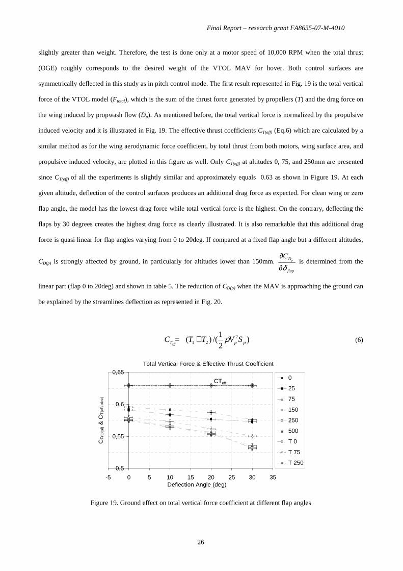
slightly greater than weight. Therefore, the test is done only at a motor speed of 10,000 RPM when the total thrust

(OGE) roughly corresponds to the desired weight of the VTOL MAV for hover. Both control surfaces are

symmetrically deflected in this study as in pitch control mode. The first result represented in Fig. 19 is the total vertical

force of the VTOL model (Ftotal), which is the sum of the thrust force generated by propellers (T) and the drag force on

the wing induced by propwash flow (Dp). As mentioned before, the total vertical force is normalized by the propulsive

induced velocity and it is illustrated in Fig. 19. The effective thrust coefficients CT(eff) (Eq.6) which are calculated by a

similar method as for the wing aerodynamic force coefficient, by total thrust from both motors, wing surface area, and

propulsive induced velocity, are plotted in this figure as well. Only CT(eff) at altitudes 0, 75, and 250mm are presented

since CT(eff) of all the experiments is slightly similar and approximately equals 0.63 as shown in Figure 19. At each

given altitude, deflection of the control surfaces produces an additional drag force as expected. For clean wing or zero

flap angle, the model has the lowest drag force while total vertical force is the highest. On the contrary, deflecting the

flaps by 30 degrees creates the highest drag force as clearly illustrated. It is also remarkable that this additional drag

force is quasi linear for flap angles varying from 0 to 20deg. If compared at a fixed flap angle but a different altitudes,

CD(p) is strongly affected by ground, in particularly for altitudes lower than 150mm. flap

DpC

δ∂

∂ is determined from the

linear part (flap 0 to 20deg) and shown in table 5. The reduction of CD(p) when the MAV is approaching the ground can

be explained by the streamlines deflection as represented in Fig. 20.

)21

/()( 221 ppT SVTTC

effρ+= (6)

Total Vertical Force & Effective Thrust Coefficient

CTeff.

0,5

0,55

0,6

0,65

-5 0 5 10 15 20 25 30 35Deflection Angle (deg)

CF

(tot

al) &

CT

(effe

ctiv

e)

0

25

75

150

250

500

T 0

T 75

T 250

Figure 19. Ground effect on total vertical force coefficient at different flap angles


27

As illustrated in Fig. 20-left, the presence of ground produces two effects. In the IGE zone (represented by circles),

flow is decelerated and spread out due to the ground plane which perpendicularly obstructs flow just under the

propeller disc. Therefore, the streamline curvature is changed, resulting in a local reduction of control surface angle. In

addition, local velocity is also reduced and a stagnation point is found at the centerline. Combining both effects, the

aerodynamic force on control surfaces IGE is decreased. When OGE, the control surfaces have normal efficiency since

they are not influenced by the ground. The reduction of download or drag force can also be explained by the reduction

of flow speed and the modification of local streamline flow IGE. Skin friction drag force of a hovering VTOL MAV is

reduced by ground effect, in particularly on the trailing part, due to the change of local skin friction coefficient and the

decreasing of local flow speed. Aerodynamic coefficients for lift force (CLp) or normal force on the wing are plotted in

Fig. 21-top and the aerodynamic derivative of lift is presented on the second line of table 5 as well. Ground has a

significant influence particularly for altitudes less than 150mm. At the same time, the control surface efficiency is

decreased when the MAV is approaching the ground.

Figure 20. Present propulsive stream line through VTOL MAV, IGE and OGE

Table 5 Aerodynamic derivatives of VTOL MAV

Altitude (measured from trailing edge to ground in mm) Aerodynamic

Derivatives

[ ×10-3 deg-1] 0 25 75 150 250 500


28

flapDpC δ∂∂ 0.4 0.74 0.89 0.89 1.08 1.10

flapLpC δ∂∂ 1.74 2.28 4.13 4.69 5.05 5.23

flapmpC δ∂∂ 0.73 -0.52 -0.80 -1.25 -1.52 -1.55

flapl pC δ∂∂ -0.68 -0.33 0.13 -0.34 0.15 -0.63

flapnpC δ∂∂ 0.19 -0.33 -1.04 -0.31 -1.06 -0.28

The pitching moment in Fig. 22 is not clearly observed when the vehicle is close to the ground as seen by its value at

an altitude of 0 and 25mm. The result is very close to zero and it is very small compared to the measurement error.

However, the pitching moment efficiency of control surface is improved when the altitude increases.

Propulsive Lift Coefficient (Normal to wing plane)

0

0,04

0,08

0,12

0,16

0,2


CL

p

0 25 75

150 250 500

Figure 21. Ground effect on lift coefficients at different flap angles


29

Propulsive Pitching Coefficient

-0,1

-0,08

-0,06

-0,04

-0,02

0

0,02

0,04

-5 0 5 10 15 20 25 30 35

Deflection Angle (deg)

Cm

p

0 25 75 150 250 500

Figure 22. Ground effect on pitching moment coefficients at different flap angles

Ground effect on roll and yaw moments are examined in this study as well. However the result is not clearly visible

as shown in Fig. 23&24. These moment coefficients are very small compared with the error and the precision of the

measurement. On Fig. 23, which shows rolling characteristics, the data are scattered around a zero value. Although, on

Fig. 24, some measured values for the yaw moment are large, the data are scattered close to zero as well. This

unexpected result may be due to small differences of thrust on the right and left propellers.

Propulsive Rolling Coefficient

-0,04

-0,03

-0,02

-0,01

0

0,01

0,02

0,03

0,04


Rol

ling

Coe

ffic

ient

; C

lp

0 25 75 150 250 500

Figure 23. Ground effect on roll coefficient at different flap angles


30

Propulsive Yaw Coefficient

-0,04

-0,03

-0,02

-0,01

0

0,01

0,02

0,03

0,04


CN

p

0 25 75 150 250 500

Figure 24. Ground effect on yaw coefficient at different flap angles

Ground has a strong effect on the efficiency of control surfaces during hover close to the ground. As explained

above, there is a change of flow speed and direction when propulsive jet flow impinges upon the ground. This

phenomenon modifies aerodynamic characteristics of the present VTOL MAV, in particular drag, lift, and pitching.

Because control surfaces of the MAVion are installed along the wing trailing edge, they can get very close to the ground

when landing if short landing legs are used. The characteristics of control efficiencies of this tail sitter VTOL MAV are

highly affected by ground effect especially when the tail-to-ground distance is less than 150mm, slightly more than the

propeller diameter.

5. CONCLUSION

An experimental study of ground effect on a new tail-sitter VTOL MAV, called MAVion, has been performed at

ISAE and is discussed in this paper. The tests are conducted using a newly acquired 5-component mini sting-balance

MicroB. Propulsive performance, aerodynamic characteristics, and efficiency of the control surfaces are examined both

IGE and OGE. The validation of a new balance, MicroB, performed by numerous tests. The error of the balance and

system are found and analyzed. The validation test demonstrates that the new balance has sufficient accuracy compared

with the full scale capacity of the balance. The minimum error is on the order of 0.01N (about 1g.) for force and it is

around 0.001N.m (about 10g.cm) for moment. The validation also found that there is no significant effect on all 5

components when applying axial force. A comparison of accuracy for the MicroB, the sting balance of the U. of Florida

and the old MicroBalance [15] of ISAE is exhibited in Table 6. The first two balances are internal sting balance type

while the 3rd one is external balance with the balance placed under the test section and the model supported by three

struts. The accuracy of MicroBalance includes error from strut drag and model gravity correction. Both internal sting


31

balances have quite similar performance in terms of maximum load and accuracy. Balance MicroB of ISAE has

approximately 2 times of maximum Roll and Yaw moments and this introduces lower accuracy in roll and yaw

moment measurements. The MicroBalance has the best accuracy when comparing all three balances for MAV research.

However, the MicroBalance has a limitation in the maximum angle of attack and accuracy of the strut drag correction.

Table 6 Comparison of Accuracy of balance for MAV research

Balance:

Institute

MicroB:

ISAE

Sting Balance:

U. of Florida

MicroBalance:

ISAE

Type Internal Internal External -3 support

Diameter [mm] 6 7.62 -

Normal [g] 1.0E+3 / 1.023E+0 1.36E+3 / 1.02E+0 3.0E+3 / 9.0E-1

Axial [g] Not Available 9.07E+2 / 6.80E-1 2.0E+3 / 3.0E-1

Side [g] 1.0E+3 / 7.33E-1 9.07E+2 / 6.80E-1 Not Available

Roll [g cm] 5.0E+3 / 8.947E+0 2.30E+3 / 2.88E+0 1.0E+4 / 2.0E+0

Pitch [g cm] 5.0E+3 / 3.85E+0 6.91E+3 / 5.18E+0 1.0E+4 / 2.0E+0

Max.Load /

Accuracy

Yaw [g cm] 5.0E+3 / 1.398E+1 2.30E+3 / 1.73E+0 1.0E+4 / 2.0E+0

Ground has some effects on the aerodynamic characteristics of the present VTOL MAV, in particularly if the

altitude is lower than 150mm. Although ground effect has almost no influence on the performance of the propulsive

system, the ground is beneficial in terms of a wing drag force reduction. The present tail-sitter VTOL MAV produces a

drag equal to about 10% of its total weight to hover over the ground. Drag coefficient of IGE determined by propulsive

induced speed is decreased by 1/3 with respect to OGE configuration. This means that a MAV hovering IGE uses less

energy than if hovering at a higher altitude. However, this gain of energy is not very high when compared with the loss

of control surface efficiencies which is more important for controlling the vehicle. Thus, it is recommended to hover

OGE which should be about 2 times the propeller diameter for security and controllability of this vehicle.

Comparison between the current experiment and numerical simulation of ground effect on the MAVion is currently

being undertaken. The study of ground effect on MAVs holds further research challenges. The size of the ground

and/or room sometimes is not large compared to the size of the MAV, as in the case of hovering over a table in a small

room. The interaction between ground, wall, and ceiling may add more complexities to the problem of indoor flight.

Furthermore, unsteady aerodynamics of a propeller can impact hovering characteristics and stability of this kind of


32

VTOL MAV. Partial ground effect, wall effect, ceiling, size of room, and unsteady aerodynamics could be further

studied.

REFERENCES

[1] McCormick, B. W. Jr., "Aerodynamics of V/STOL Flight", Dover Publications, Inc., NY, 1999.

[2] S. Shkarayev, University of Arizona; J.-M. Moschetta, B. Bataillé, Institut Supérieur de l’Aéronautique et de l’Espace,

"Aerodynamic Design of Micro Air Vehicles for Vertical Flight", Journal of Aircraft 20080021-8669 vol.45 no.5 (1715-1724)

[3] Prouty, R. W., “Ground Effect and the Helicopter - A Summary,” AHS, and ASEE, Aircraft Design Systems and Operations

Meeting, Coloradao Springs, CO, Oct 14-16, 1985, AIAA-1985-4034.

[4] Pulla, D. P. and Conlisk, A. T., “A Lifting Surface Study of Helicopter Aerodynamics in Ground Effect,” 45th AIAA Aerospace

Science Meeting and Exhibit, Reno, Nevada, Jan 8-11, 2007, AIAA 2007-1279.

[5] Nathan, N. D. and Green, R. B., “Measurements of a Rotor Flow in Ground Effect and Visualisation of the Brown-Out

Phenomenon,” the American Helicopter Society 64th Annual Forum, Montreal, Canada, April 29 – May 1, 2008.

[6] Ganesh, B. and Komerath, N., “Study of Ground Vortex Structure of Rotorcraft in Ground Effect at Low Advance Ratios,” 24th

Applied Aerodynamics Conference, San Francisco, California, June 5-8, 2006, AIAA 2006-3475.

[7] Kotansky, D. R. and Bower, W. W., “A Basic Study of the VTOL Ground Effect Problem for Planar Flow,” Journal of

Aircraft, Vol. 15, No. 4, pp. 214-221.

[8] Campbell, J. P., Hassel, J. L., and Thomas, J. L., “Ground Effects on Lift for Turbofan Powered-Lift STOL Aircraft,” Journal

of Aircraft, Vol. 15, No. 2, pp. 78-84.

[9] Morris, S. et al., “Analysis of a Hoverwing in Ground Effect,” 46th AIAA Aerospace Science Meeting and Exhibit, Reno,

Nevada, Jan 7- 10, 2008, AIAA 2008-431.

[10] Radhakrishnan, A. and Schmitz, F. H., “An Experimental Investigation of a Quad Tilt Rotor in Ground Effect,” 21st Applied

Aerodynamics Conference, Orlando, Florida, June 23-26, 2003, AIAA 2003-3517.

[11] Radhakrishnan, A. and Schmitz, F. H., “Quad Tilt Rotor Aerodynamics in Ground Effect,” 23rd AIAA Applied Aerodynamics

Conference, Toronto, Canada, June 6-9, 2005, AIAA 2005-5218.

[12] Thipyopas, C. and Moschetta, J.M., “A Fixed-Wing Biplane MAV for Low Speed Missions,” International Journal of Micro

Air Vehicles, Vol. 1, No. 1, pp. 13-33.

[13] Phillips W. F., “Propeller Momentum Theory with Slipstream Rotation”, Journal of Aircraft, Vol. 39, n. 1, pp. 184-187

[14] Kline, S.J. and McClintock, F.A., “Describing Uncertainties in Single-Sample Experiments,” Mechanical Engineering, Vol. 1,

1953, pp. 3-8.

[15] Moschetta, J.M. and Thipyopas, C., “Aerodynamic Performance of a Biplane Micro Air Vehicle”, Journal of Aircraft, Vol.44,

No. 1, pp. 291-299.

A Fixed-Wing Micro Air Vehicle with Hovering … fixed-wing micro aerial vehicle with hover flight...

Documents

Transcript of A Fixed-Wing Micro Air Vehicle with Hovering … fixed-wing micro aerial vehicle with hover flight...