A FINITE ELEMENT IMPLEMENTATION OF …yadda.icm.edu.pl/yadda/element/bwmeta1.element.baztech...This...

T H E A R C H I V E O F M E C H A N I C A L E N G I N E E R I N G

VOL. LVIII 2011 Number 3

10.2478/v10180-011-0021-7Key words: elasticity tensor, tangent modulus tensor, material Jacobian, hyperelasticity, stored-energy potential,constitutive equation, finite element method

CYPRIAN SUCHOCKI ∗

A FINITE ELEMENT IMPLEMENTATION OF KNOWLESSTORED-ENERGY FUNCTION: THEORY, CODING AND

APPLICATIONS

This paper contains the full way of implementing a user-defined hyperelasticconstitutive model into the finite element method (FEM) through defining an ap-propriate elasticity tensor. The Knowles stored-energy potential has been chosen toillustrate the implementation, as this particular potential function proved to be veryeffective in modeling nonlinear elasticity within moderate deformations. Thus, theKnowles stored-energy potential allows for appropriate modeling of thermoplastics,resins, polymeric composites and living tissues, such as bone for example. The decou-pling of volumetric and isochoric behavior within a hyperelastic constitutive equationhas been extensively discussed. An analytical elasticity tensor, corresponding to theKnowles stored-energy potential, has been derived. To the best of author’s knowl-edge, this tensor has not been presented in the literature yet. The way of derivinganalytical elasticity tensors for hyperelastic materials has been discussed in detail.The analytical elasticity tensor may be further used to develop visco-hyperelastic,nonlinear viscoelastic or viscoplastic constitutive models. A FORTRAN 77 code hasbeen written in order to implement the Knowles hyperelastic model into a FEMsystem. The performance of the developed code is examined using an exemplaryproblem.

NOMENCLATURE

B left Cauchy-Green (C-G) deformation tensor,B isochoric left C-G deformation tensor,Br ,Bt reference and current configurations,Biso

t current configuration after purely distortional deformation,C right Cauchy-Green (C-G) deformation tensor,C isochoric right C-G deformation tensor,CCC elasticity tensor,CCCτc elasticity tensor related to convected stress rate,

∗ Warsaw University of Technology, Institute of Mechanics and Printing, ul. Narbutta 85,02-524 Warszawa, Poland; E-mail: [email protected]

320 CYPRIAN SUCHOCKI

CCCτZ−J elasticity tensor related to Zaremba-Jaumann stress rate,CCCMZ−J elasticity tensor used by Abaqus,[Ci j

]elasticity matrix used by Abaqus,

D strain rate tensor,ek unit vector of a Cartesian base, k = 1, 2, 3,F deformation gradient tensor,F isochoric deformation gradient tensor,Fvol dilatational deformation gradient tensor,H fourth order auxiliary tensor,I fourth order identity tensor,Ik algebraic invariants of the right C-G deformation tensor, k = 1, 2, 3,Ik algebraic invariants of the isochoric right C-G deformation tensor, k = 1, 2, 3,J Jacobian determinant,L velocity gradient tensor,S second Piola-Kirchhoff (P-K) stress tensor,U volumetric stored elastic energy potential,We stored elastic energy potential,W isochoric stored elastic energy potential,λk stretch ratio in the k-th direction, k = 1, 2, 3,τ,σ Kirchhoff and Cauchy stress tensors,x,X position vectors in the current and in the reference configuration,1, δi j second order identity tensor in the absolute and indicial notation,µ, b, n,D1 material parameters,DEV[•] operator extracting deviatoric part of a tensor in reference configuration,Grad(•) operator of a gradient with respect to X,Lv(•) convected objective rate operator,tr(•) trace operator,(•)T transpose operator,· double contraction operator,⊗ dyadic product operator,(•)∇ Zaremba-Jaumann (Z-J) objective rate operator.

1. Introduction

Numerous materials such as thermoplastics, resins or polymeric compos-ites exhibit nonlinear elastic behavior for strains ranging up to 5%. In orderto take this phenomenon into account in the Finite Element Analysis (FEA),a proper hyperelastic constitutive model has to be employed.

As it has been observed by several researchers [3], [21], the popularmodels of hyperelasticity like Neo-Hooke or Mooney-Rivlin for instance,which are very effective in modeling large strain nonlinear elasticity, are notable to capture the nonlinear elastic behavior in the range up to 5%. Thisproblem is usually skipped by making use of the linear elastic model (Saint-Venant-Kirchhoff stored-energy potential) or/and assuming that the entirenonlinearity is due to plasticity. This assumption is in contradiction to theexperimental observations. In the case of thermoplastic polymers for example,it can be noticed that after a loading-unloading experiment a certain strain

A FINITE ELEMENT IMPLEMENTATION... 321

remains in the specimen in face of a zero stress. It should be noticed, however,that the remaining strain is not plastic but viscoelastic, and it decreases asthe specimen rests, to finally vanish after a properly long time period. Thiskind of behavior is typical for viscoelastic materials, and it is usually statedthat this group of materials does not posses a well-defined stress free state. Inother words, the stress free state of the specimen may occur at different statesof deformation. Since the deformations are elastic, they should be modeledas such, and assuming that they are plastic is a mistake.

stre

ss [

MP

a]

stretch [-]

experiment

S V-K

N-H

K

Fig. 1. Simple tension test data and theoretical predictions

It has been already mentioned that the popular models of hyperelasticityfail to capture the experimental stress-strain curve of the materials which ex-hibit nonlinear elasticity for moderate strains. The theoretical predictions ofSaint Venant-Kirchhoff (S V-K), Neo-Hooke (N-H) and Knowles (K) modelsare compared in the Figure 1 to the experimental results of a simple tensiontest performed on a specimen of high density polyethylene [7]. A proper setof material constants can allow for good description of small strain behavior,as it can be seen for the Saint Venant-Kirchhoff model. Further predictionscarry a significant error which can range over 50%. Improving the modelpredictions for higher strains results in increasing the error in the range ofsmall strains, as it has been shown for Neo-Hooke model. Thus, a stored-energy potential that would effectively describe the stress-strain relation isneeded. For that purpose several researchers have proposed various, alter-native stored-energy potentials. Bouchart proposed using Ciarlet-Geymonatstored-energy function in order to model the elastic response of polyprophy-lene [3]. This model uses four material constants and all three invariants ofthe right Cauchy-Green (C-G) deformation tensor. It appears that Knowlesstored-energy potential [11], used by Soares and Rajagopal to model poly-lactide [22], is a better solution. The model by Knowles uses four material


constants but only one invariant (first) of the right C-G deformation tensorwhich simplifies the process of material parameter identification. As it canbe seen in Figure 1, the Knowles model allows for effective modeling ofelastic response of thermoplastics, resins, polymeric composites, metals andliving tissues such as bone for example.

The model by Knowles is not offered by any of the popular FEA systemsand, in order to use it, one has to implement it as a user-defined material.In this study, the full way of implementing the Knowles material model intoFEA system Abaqus has been presented. The focus on Abaqus system doesnot cause a loss in generality as the general framework of implementing auser-defined material is similar in all FEA systems.

A user-defined hyperelastic constitutive laws can be implemented intoAbaqus in several ways. Abaqus offers three alternative user subroutineswhich can be used for implementing a hyperelastic constitutive equation.Those are: UHYPER (for isotropic incompressible hyperelastic materials),UANISOHYPER (for anisotropic hyperelastic materials) and UMAT (generalpurpose subroutine which can be used for implementing arbitrary materialbehavior). Abaqus allows for using both UHYPER and UANISOHYPER todevelop a more sophisticated constitutive equations. Both subroutines can beused to model nonlinear viscoelasticity within a theory which is similar to thePipkin & Rogers theory of viscoelasticity [5]. Alternatively, Mullins effectcan be modeled together with the elastic response defined by a user subroutine(viscoelasticity and Mullins effect must be used separately; Abaqus doesnot allow for combining those behaviors). Thus, a user implementing hisconstitutive equation through sobroutines UHYPER or UANISOHYPER islimited to using built in options of Abaqus.

In order to develop a constitutive equation based on the theories notsupported by Abaqus, subroutine UMAT should be used. Using subroutineUMAT requires defining material stiffnes tensor also reffered to as tangentmodulus tensor, material Jacobian or elasticity tensor in the case of elasticmaterials. The derivation of an analytical elasticity tensor is not an easytask, which is the reason why the approximate elasticity tensors are oftenused, although they worsen the rate of convergence and accuracy of analysis’results. Stein and Sagar [23] have found for the Neo-Hooke hyperelasticmodel that only an analytically derived elasticity tensor assures a quadraticrate of convergence1. For the approximate elasticity tensors, not only theconvergence rates are not quadratic but even convergence at all is not assured

1 Quadratic convergence means that the square of the error at one iteration is proportionalto the error at the next iteration.


for all elements and considered problems. Thus, it is always profitable to usean analytical elasticity tensor whenever it is possible.

This paper presents the entire way of derivation of an analytical elasticitytensor corresponding to the Knowles stored-energy potential. To the best ofauthor’s knowledge, this tensor has not been reported in the literature yet. Itshould be noted that the discussed framework is valid for both isotropic andanisotropic hyperelastic materials.

2. Kinematics of finite deformations

Let us consider a continuum body whose reference configuration is de-noted as Br . As a consequence of the deformation, the body takes a new(current) configuration denoted as Bt (Fig. 2).

Fig. 2. Deformation gradient F

The position vectors of a considered particle are denoted as X and x inthe reference and current configurations, respectively. It is assumed that aone-to-one mapping function of the form x = χ(X, t) exists.

The deformation gradient F is as second order tensor which is definedby the following equation:

F = Grad x (X, t) (1)

where „Grad” denotes a gradient operation with respect to the componentsof vector X. The Cartesian components of F are Fi j = ∂xi/∂X j (i, j=1,2,3).

During the motion, a spatial velocity field may be expressed as v(x, t) =

∂x/∂t and a velocity gradient tensor can be defined as L = FF−1. As anyother second order tensor, L can be decomposed into a sum of a symmetric

and an antisymmetric tensors, namely L = D + W, where D =12

(L + LT

)is

the strain rate tensor and W =12

(L − LT

)is the spin tensor. The symmetric


Fig. 3. Alternative paths of deformation

and positive-definite right and left Cauchy-Green (C-G) deformation tensorsare defined as C = FTF and B = FFT , respecively.

For the use of finite element method it is worthy to decouple the di-latational (volumetric) and distortional (isochoric) deformations. This can beachieved by a multiplicative decomposition of the deformation gradient [9]:

F = FvolF (2)

where Fvol denotes a deformation gradient corresponding to purely volu-metric deformation (Fvol = J1/31) and F denotes a deformation gradientcorresponding to purely isochoric deformation (F = J−1/3F). J = det F is theJacobian determinant also known as the volume ratio. Figure 3 provides agraphic interpretation of the considered multiplicative decomposition. Otherdeformation tensors can be decomposed in a similar way. The right and leftCauchy-Green (C-G) deformation tensors are decomposed as [9]:

C = FTF = J2/3C, B = FFT = J2/3B (3)

where C = FTF and B = FF

Tare the right and left volume-preserving C-G

deformation tensors, respecively.

3. Decoupled constitutive equation of hyperelastic material

A hyperelastic or Green elastic material is defined as an elastic materialwhich possesses a stored elastic energy function, denoted as We [9], [15], [16].


From the principles of conservation of energy and conservation of angularmomentum the following expression for the time derivative of the stored-energy potential can be obtained [24]:

We = S · E =12S · C (4)

where S is the second Piola-Kirchhoff (P-K) stress tensor, E is the Greenfinite strain tensor and C is the right Cauchy-Green (C-G) deformation tensor.After assuming that We = We(C) and applying the chain rule to (4), it is foundthat: (

S − 2∂We

∂C

)· 12C = 0 (5)

which holds for arbitrary C. Thus it can be deduced that:

S = 2∂We

∂C(6)

which is the general form of the constitutive equation determining the relationbetween stress and deformation tensors for a hyperelastic material.

For the isotropic hyperelastic materials, We may be regarded as a functionof the three principal algebraic invariants I1, I2, I3 of C, namely:

We(C) = We(I1, I2, I3) (7)

in order to fulfill the requirements of objectivity and isotropy.The invariants of the right C-G deformation tensor are given by the

following formulas:

I1 = tr C, I2 =12

((tr C)2 − tr C2

), I3 = J2 = det C (8)

where tr (•) is the trace operator and J is the Jacobian determinant.In terms of FEM, it is profitable if the volumetric and isochoric responses

are decoupled within the constitutive equation. The decoupling siginificantlysimplifies the derivation and the final form of the fourth-order elasticity ten-sor. It is facilitated by assuming a stored-energy function of the form [9], [25]:

We(C) = U(J) + W (C) (9)

where U and W are volumetric and isochoric stored-energy potentials, re-spectively. The enforcement of incompressibility constraint is much easier foran uncoupled stored-energy, as it is achieved simply by assuming a properlyhigh value of the bulk modulus.


In order to find a general form of a constitutive equation correspondingto a stored-energy potential given by (9), the following results are needed:

∂J∂C

=12JC−1,

∂C∂C

= J−2/3(I − 1

3C ⊗ C−1

). (10)

By substituting stored-energy potential (9) into (6), making use of the chainrule and the results (10), it is in turn found that:

S = 2∂U∂J

∂J∂C

+ 2∂W

∂C· ∂C∂C

= J∂U∂J

C−1 + 2J−2/3∂W

∂C·(I − 1

3C ⊗ C

−1)

= J∂U∂J

C−1 + 2J−2/3∂W∂C− 1

3

∂W∂C· C

C−1

After introducing the following operator [25]:

DEV [•] = [•] − 13

([•] · C

)C−1

(11)

which extracts the deviatoric part from a second order tensor in the referenceconfiguration, the above lengthty result can be significantly shortened, thatis:

S = J∂U∂J

C−1 + 2J−2/3 DEV∂W∂C

. (12)

It should be emphasized that the equation (12) is valid for both isotropic andanisotropic materials.

In the special case of the isotropic hyperelastic materials, the stored-energy potential takes the form:

We(C) = U(J) + W (I1, I2) (13)

where I1 = J−2/3I1 and I2 = J−4/3I2. Depending on the values of the materialparameters associated with the volumetric potential U(J), equation (12) candescribe compressible, slightly comressible or almost-incompressible mate-rial.


4. Uncoupled elasticity tensor and objective rate of stress tensor

The nonlinear constitutive equation defined by (6) can be transformedinto the following incremental2 form [2], [9], [14]:

∆S = CCC · 12

∆C (14)

which is a linear relation between the increments of S and C, and so it iscommonly referred to as linearized constitutive equation. CCC denotes a fourth-order elasticity tensor, defined as:

CCC = 2∂S∂C

= 4∂2We

∂C∂C. (15)

Substituting the equation (12) into (15) gives [25]:

CCC = 2∂S∂C

= 2∂

∂C

(2∂We

∂C

)

= 2∂

∂C

J∂U∂J

C−1 + 2J−2/3∂W∂C− 1

3

∂W∂C· C

C−1

.

(16)

Having in mind the results (10) and additionally∂C−1

∂C= −IC−1 , where

(IC−1)i jkl = −12

(C−1ik C−1jl + C−1il C−1jk

), a systematic use of the chain rule leads

to an expression3:

CCC = J∂U∂J

(C−1 ⊗ C−1 − 2IC−1

)+ J2∂

2U∂J2 C−1 ⊗ C−1

− 43J−4/3

∂W∂C⊗ C

−1+ C

−1 ⊗ ∂W∂C

+43J−4/3

∂W∂C· C

(J4/3IC−1 +

13C−1 ⊗ C

−1)

+ J−4/3CCCW

(17)

2 Starting off from this section some differentials met in the formulas have been replacedwith finite increments as they are implemented as such into FEM.

3 see Appendix B. for the derivation.


where CCCW is the part of CCC which arises directly from the second derivativesof W with respect to C [25]. It is defined as:

CCCW = 4∂2W

∂C∂C− 4

3

∂

2W

∂C∂C· C

⊗ C−1

+ C−1 ⊗

C · ∂2W

∂C∂C

+49

C · ∂2W

∂C∂C· C

C−1 ⊗ C

−1.

(18)

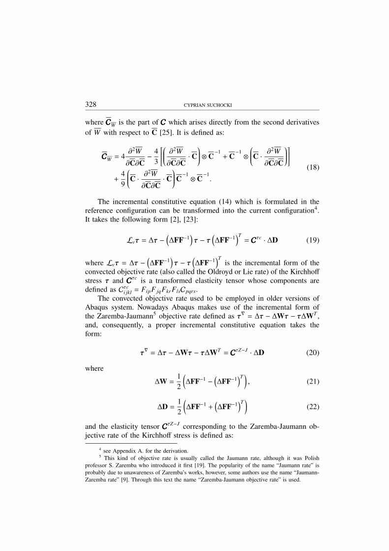
The incremental constitutive equation (14) which is formulated in thereference configuration can be transformed into the current configuration4.It takes the following form [2], [23]:

Lvτ = ∆τ −(∆FF−1

)τ − τ

(∆FF−1

)T= CCCτc · ∆D (19)

where Lvτ = ∆τ −(∆FF−1

)τ − τ

(∆FF−1

)Tis the incremental form of the

convected objective rate (also called the Oldroyd or Lie rate) of the Kirchhoffstress τ and CCCτc is a transformed elasticity tensor whose components aredefined as Cτci jkl = FipF jqFkrFlsCpqrs.

The convected objective rate used to be employed in older versions ofAbaqus system. Nowadays Abaqus makes use of the incremental form ofthe Zaremba-Jaumann5 objective rate defined as τ∇ = ∆τ − ∆Wτ − τ∆WT ,and, consequently, a proper incremental constitutive equation takes theform:

τ∇ = ∆τ − ∆Wτ − τ∆WT = CCCτZ−J · ∆D (20)

where

∆W =12

(∆FF−1 −

(∆FF−1

)T ), (21)

∆D =12

(∆FF−1 +

(∆FF−1

)T )(22)

and the elasticity tensor CCCτZ−J corresponding to the Zaremba-Jaumann ob-jective rate of the Kirchhoff stress is defined as:

4 see Appendix A. for the derivation.5 This kind of objective rate is usually called the Jaumann rate, although it was Polish

professor S. Zaremba who introduced it first [19]. The popularity of the name “Jaumann rate” isprobably due to unawareness of Zaremba’s works, however, some authors use the name “Jaumann-Zaremba rate” [9]. Through this text the name “Zaremba-Jaumann objective rate” is used.


CCCτZ−J = CCCτc +12

(δikτ jl + τikδ jl + δilτ jk + τilδ jk

)ei ⊗ e j ⊗ ek ⊗ el (23)

where ek (k = 1, 2, 3) denotes a unit vector of a Cartesian basis.It should be noted that the elasticity tensor which should be implemented

into the subroutine UMAT is slightly different from (23) and takes the form:

CCCMZ−J =1JCCCτZ−J . (24)

The framework presented above can be used to derive the analytical elasticitytensors of both isotropic and anisotropic hyperelastic materials.

5. Abaqus implementation

5.1. General

In the following text the analytical elasticity tensor following from theKnowles hyperelastic model is presented. The derived analytical elasticitytensor has been implemented into the Abaqus system via subroutine UMAT.

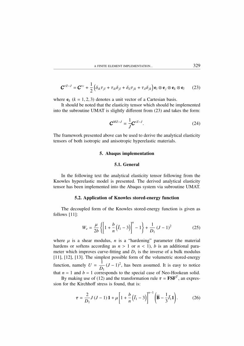
5.2. Application of Knowles stored-energy function

The decoupled form of the Knowles stored-energy function is given asfollows [11]:

We =µ

2b

{[1 +

bn

(I1 − 3

)]n− 1

}+

1D1

(J − 1)2 (25)

where µ is a shear modulus, n is a “hardening” parameter (the materialhardens or softens according as n > 1 or n < 1), b is an additional para-meter which improves curve-fitting and D1 is the inverse of a bulk modulus[11], [12], [13]. The simplest possible form of the volumetric stored-energy

function, namely U =1D1

(J − 1)2, has been assumed. It is easy to notice

that n = 1 and b = 1 corresponds to the special case of Neo-Hookean solid.By making use of (12) and the transformation rule τ = FSFT , an expres-

sion for the Kirchhoff stress is found, that is:

τ =2D1

J (J − 1) 1 + µ

[1 +

bn

(I1 − 3

)]n−1 (B − 1

3I11

). (26)


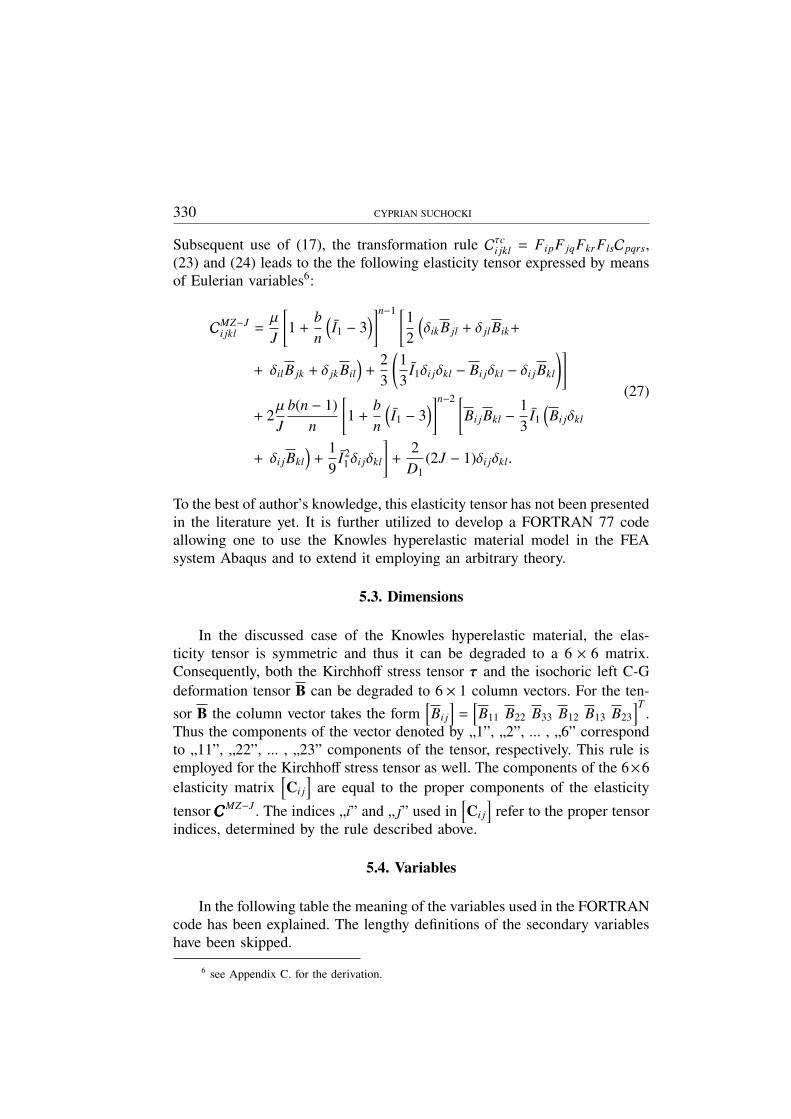
Subsequent use of (17), the transformation rule Cτci jkl = FipF jqFkrFlsCpqrs,(23) and (24) leads to the the following elasticity tensor expressed by meansof Eulerian variables6:

CMZ−Ji jkl =

µ

J

[1 +

bn

(I1 − 3

)]n−1 [12

(δikB jl + δ jlBik+

+ δilB jk + δ jkBil

)+

23

(13I1δi jδkl − Bi jδkl − δi jBkl

)]

+ 2µ

Jb(n − 1)

n

[1 +

bn

(I1 − 3

)]n−2 [Bi jBkl − 1

3I1

(Bi jδkl

+ δi jBkl

)+

19I21δi jδkl

]+

2D1

(2J − 1)δi jδkl.

(27)

To the best of author’s knowledge, this elasticity tensor has not been presentedin the literature yet. It is further utilized to develop a FORTRAN 77 codeallowing one to use the Knowles hyperelastic material model in the FEAsystem Abaqus and to extend it employing an arbitrary theory.

5.3. Dimensions

In the discussed case of the Knowles hyperelastic material, the elas-ticity tensor is symmetric and thus it can be degraded to a 6 × 6 matrix.Consequently, both the Kirchhoff stress tensor τ and the isochoric left C-Gdeformation tensor B can be degraded to 6 × 1 column vectors. For the ten-sor B the column vector takes the form

[Bi j

]=

[B11 B22 B33 B12 B13 B23

]T.

Thus the components of the vector denoted by „1”, „2”, ... , „6” correspondto „11”, „22”, ... , „23” components of the tensor, respectively. This rule isemployed for the Kirchhoff stress tensor as well. The components of the 6×6elasticity matrix

[Ci j

]are equal to the proper components of the elasticity

tensor CCCMZ−J . The indices „i” and „ j” used in[Ci j

]refer to the proper tensor

indices, determined by the rule described above.

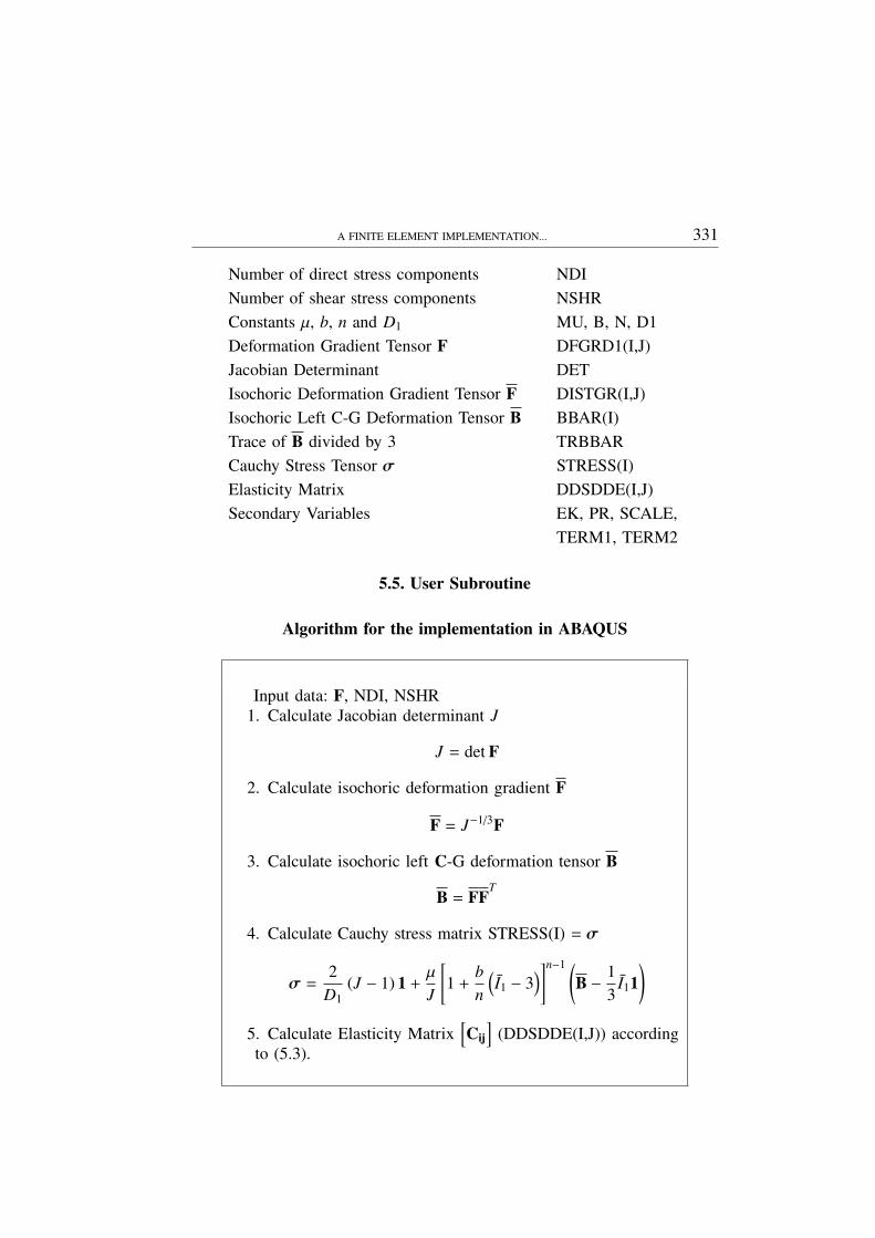
5.4. Variables

In the following table the meaning of the variables used in the FORTRANcode has been explained. The lengthy definitions of the secondary variableshave been skipped.

6 see Appendix C. for the derivation.


Number of direct stress components NDINumber of shear stress components NSHRConstants µ, b, n and D1 MU, B, N, D1Deformation Gradient Tensor F DFGRD1(I,J)Jacobian Determinant DETIsochoric Deformation Gradient Tensor F DISTGR(I,J)Isochoric Left C-G Deformation Tensor B BBAR(I)Trace of B divided by 3 TRBBARCauchy Stress Tensor σ STRESS(I)Elasticity Matrix DDSDDE(I,J)Secondary Variables EK, PR, SCALE,

TERM1, TERM2

5.5. User Subroutine

Algorithm for the implementation in ABAQUS

Input data: F, NDI, NSHR1. Calculate Jacobian determinant J

J = det F

2. Calculate isochoric deformation gradient F

F = J−1/3F

3. Calculate isochoric left C-G deformation tensor B

B = FFT

4. Calculate Cauchy stress matrix STRESS(I) = σ

σ =2D1

(J − 1) 1 +µ

J

[1 +

bn

(I1 − 3

)]n−1 (B − 1

3I11

)

5. Calculate Elasticity Matrix[Cij

](DDSDDE(I,J)) according

to (5.3).


5.6. Coding in FORTRAN 77

SUBROUTINE UMAT(STRESS,STATEV,DDSDDE,SSE,SPD,SCD,1 RPL,DDSDDT,DRPLDE,DRPLDT,STRAN,DSTRAN,2 TIME,DTIME,TEMP,DTEMP,PREDEF,DPRED,MATERL,NDI,NSHR,NTENS,3 NSTATV,PROPS,NPROPS,COORDS,DROT,PNEWDT,CELENT,4 DFGRD0,DFGRD1,NOEL,NPT,KSLAY,KSPT,KSTEP,KINC)

CINCLUDE ’ABA PARAM.INC’

CCHARACTER*8 MATERLDIMENSION STRESS(NTENS),STATEV(NSTATV),1 DDSDDE(NTENS,NTENS),DDSDDT(NTENS),DRPLDE(NTENS),2 STRAN(NTENS),DSTRAN(NTENS),DFGRD0(3,3),DFGRD1(3,3),3 TIME(2),PREDEF(1),DPRED(1),PROPS(NPROPS),COORDS(3),DROT(3,3)

CC LOCAL ARRAYSC - - - - - - - - - - - - - - - - - - - - - - - - - - - - - - - - - - - - - - - - - - - - - - - - -C BBAR - DEVIATORIC RIGHT CAUCHY-GREEN TENSORC DISTGR - DEVIATORIC DEFORMATION GRADIENT (DISTORTION TENSOR)C - - - - - - - - - - - - - - - - - - - - - - - - - - - - - - - - - - - - - - - - - - - - - - - - -C

DIMENSION BBAR(6),DISTGR(3,3)C

PARAMETER(ZERO=0.D0, ONE=1.D0, TWO=2.D0, THREE=3.D0, FOUR=4.D0)CC - - - - - - - - - - - - - - - - - - - - - - - - - - - - - - - - - - - - - - - - - - - - - - - - -C UMAT FOR COMPRESSIBLE KNOWLES HYPERELASTICITYCC WARSAW UNIVERSITY OF TECHNOLOGYCC CYPRIAN SUCHOCKI, MAY 2011C - - - - - - - - - - - - - - - - - - - - - - - - - - - - - - - - - - - - - - - - - - - - - - - - -C FOR LOW D1 HYBRID ELEMENTS SHOULD BE USEDC - - - - - - - - - - - - - - - - - - - - - - - - - - - - - - - - - - - - - - - - - - - - - - - - -C PROPS(1) - MUC PROPS(2) - BC PROPS(3) - NC PROPS(4) - D1C - - - - - - - - - - - - - - - - - - - - - - - - - - - - - - - - - - - - - - - - - - - - - - - -

REAL MU, B, N, D1, TERM1, TERM2CC ELASTIC PROPERTIESC

MU=264.069B=54.19N=0.2554D1 =0.000000033

CC JACOBIAN AND DISTORTION TENSORC

DET=DFGRD1(1, 1)*DFGRD1(2, 2)*DFGRD1(3, 3)1 -DFGRD1(1, 2)*DFGRD1(2, 1)*DFGRD1(3, 3)IF(NSHR.EQ.3) THENDET=DET+DFGRD1(1, 2)*DFGRD1(2, 3)*DFGRD1(3, 1)1 +DFGRD1(1, 3)*DFGRD1(3, 2)*DFGRD1(2, 1)2 -DFGRD1(1, 3)*DFGRD1(3,1)*DFGRD1(2, 2)3 -DFGRD1(2, 3)*DFGRD1(3, 2)*DFGRD1(1, 1)


END IFSCALE=DET**(-ONE/THREE)DO K1=1, 3

DO K2=1, 3DISTGR(K2, K1)=SCALE*DFGRD1(K2, K1)

END DOEND DO

CC CALCULATE LEFT CAUCHY-GREEN TENSORC

BBAR(1)=DISTGR(1, 1)**2+DISTGR(1, 2)**2+DISTGR(1, 3)**2BBAR(2)=DISTGR(2, 1)**2+DISTGR(2, 2)**2+DISTGR(2, 3)**2BBAR(3)=DISTGR(3, 3)**2+DISTGR(3, 1)**2+DISTGR(3, 2)**2BBAR(4)=DISTGR(1, 1)*DISTGR(2, 1)+DISTGR(1, 2)*DISTGR(2, 2)1 +DISTGR(1, 3)*DISTGR(2, 3)IF(NSHR.EQ.3) THENBBAR(5)=DISTGR(1, 1)*DISTGR(3, 1)+DISTGR(1, 2)*DISTGR(3, 2)1 +DISTGR(1, 3)*DISTGR(3, 3)BBAR(6)=DISTGR(2, 1)*DISTGR(3, 1)+DISTGR(2, 2)*DISTGR(3, 2)1 +DISTGR(2, 3)*DISTGR(3, 3)END IF

CC CALCULATE THE STRESSC

TRBBAR=(BBAR(1)+BBAR(2)+BBAR(3))/THREETERM1=MU/DET*(ONE+B/N*(THREE*TRBBAR-THREE))**(N-ONE)TERM2=TWO*MU/DET*B*(N-ONE)/N*(ONE+B/N*(THREE*TRBBAR-THREE))**(N1 -TWO)EK=TWO/D1*(TWO*DET-ONE)PR=TWO/D1*(DET-ONE)DO K1=1,NDI

STRESS(K1)=TERM1*( BBAR(K1)-TRBBAR)+PREND DODO K1=NDI+1,NDI+NSHR

STRESS(K1)=TERM1*BBAR(K1)END DO

CC CALCULATE THE STIFFNESSC

EG23=EG*TWO/THREEDDSDDE(1, 1)=TWO/THREE*TERM1*(BBAR(1)+TRBBAR)+1 TERM2*(BBAR(1)**TWO-TWO*TRBBAR*BBAR(1)+TRBBAR**TWO)+EKDDSDDE(2, 2)=TWO/THREE*TERM1*(BBAR(2)+TRBBAR)+1 TERM2*(BBAR(2)**TWO-TWO*TRBBAR*BBAR(2)+TRBBAR**TWO)+EKDDSDDE(3, 3)=TWO/THREE*TERM1*(BBAR(3)+TRBBAR)+1 TERM2*(BBAR(3)**TWO-TWO*TRBBAR*BBAR(3)+TRBBAR**TWO)+EKDDSDDE(1, 2)=TWO/THREE*TERM1*(TRBBAR-BBAR(1)-1 BBAR(2))+TERM2*(BBAR(1)*BBAR(2)-2 TRBBAR*(BBAR(1)+BBAR(2))+TRBBAR**TWO)+EKDDSDDE(1, 3)=TWO/THREE*TERM1*(TRBBAR-BBAR(3)-1 BBAR(1))+TERM2*(BBAR(3)*BBAR(1)-TRBBAR*(BBAR(3)+2 BBAR(1))+TRBBAR**TWO)+EKDDSDDE(2, 3)=TWO/THREE*TERM1*(TRBBAR-BBAR(2)-BBAR(3))+1 TERM2*(BBAR(2)*BBAR(3)-TRBBAR*(BBAR(2)+BBAR(3))+2 TRBBAR**TWO)+EKDDSDDE(1, 4)=ONE/THREE*TERM1*BBAR(4)+TERM2*(BBAR(1)-1 TRBBAR)*BBAR(4)DDSDDE(2, 4)=ONE/THREE*TERM1*BBAR(4)+TERM2*(BBAR(2)-1 TRBBAR)*BBAR(4)


DDSDDE(3, 4)=-TWO/THREE*TERM1*BBAR(4)+TERM2*(BBAR(3)-1 TRBBAR)*BBAR(4)DDSDDE(4, 4)=ONE/TWO*TERM1*(BBAR(1)+BBAR(2))IF(NSHR.EQ.3) THENDDSDDE(1, 5)=ONE/THREE*TERM1*BBAR(5)+TERM2*(BBAR(1)-1 TRBBAR)*BBAR(5)DDSDDE(2, 5)=-TWO/THREE*TERM1*BBAR(5)+TERM2*(BBAR(2)-1 TRBBAR)*BBAR(5)DDSDDE(3, 5)=ONE/THREE*TERM1*BBAR(5)+TERM2*(BBAR(3)-1 TRBBAR)*BBAR(5)DDSDDE(1, 6)=-TWO/THREE*TERM1*BBAR(6)+TERM2*(BBAR(1)-1 TRBBAR)*BBAR(6)DDSDDE(2, 6)=ONE/THREE*TERM1*BBAR(6)+TERM2*(BBAR(2)-1 TRBBAR)*BBAR(6)DDSDDE(3, 6)=ONE/THREE*TERM1*BBAR(6)+TERM2*(BBAR(3)-1 TRBBAR)*BBAR(6)DDSDDE(5, 5)=ONE/TWO*TERM1*(BBAR(3)+BBAR(1))+1 TERM2*BBAR(5)**TWODDSDDE(6, 6)=ONE/TWO*TERM1*(BBAR(3)+BBAR(2))+1 TERM2*BBAR(6)**TWODDSDDE(4,5)=ONE/TWO*TERM1*BBAR(6)+TERM2*BBAR(4)*BBAR(5)DDSDDE(4,6)=ONE/TWO*TERM1*BBAR(5)+TERM2*BBAR(4)*BBAR(6)DDSDDE(5,6)=ONE/TWO*TERM1*BBAR(4)+TERM2*BBAR(5)*BBAR(6)END IFDO K1=1, NTENS

DO K2=1, K1-1DDSDDE(K1, K2)=DDSDDE(K2, K1)

END DOEND DO

CRETURNEND

6. Performance

In order to verify the performance of the code presented above, a simu-lation of a uniaxial tension experiment has been conducted in FEA systemAbaqus, version 6.8. The simulation utilized a single finite element C3D8H7.It has been assumed that the material is almost ideally incompressible.

The displacement vector components at each of the nodes have beendisplayed in Figure 4. The i-th (i = 1, 2, 3) displacement vector componentat j-th ( j = 1, 2, . . . , 8) node has been denoted as u j

i . The u j1 displacement

components (direction „1”) have been set to ∆u for the nodes 5, 6, 7 and 8,whereas some displacements have been fixed to equal zero in order to excludethe possibility of rigid body motion. The employed set of boundary conditionsallowed for obtaining the state of uniaxial tension in the entire volume ofthe finite element. Due to the assumed incompressibility the deformationgradient corresponding to the given deformation process takes the form:

7 cubic, three-dimensional, 8 nodes, hybrid.


Fig. 4. Boundary conditions used for single element uniaxial tension test

Fig. 5. Comparison of simple tension test data and FEM predictions

[F] =

λ1 0 0

01√λ1

0

0 01√λ1

where λ1 denotes the stretch ratio in the direction „1”.The data obtained from a uniaxial tension test performed on high density

polyethylene (HDPE) [7] at the deformation rate of 0.004 s−1 [7] were usedto determine the constants µ, b and n. The inverse of the bulk modulus D1has been set to 0.000000033 MPa−1 in order to account for almost incom-pressible deformation. In Figure 5 the theoretical predictions of the FEM


simulation have been compared to the experimental data. It can be seen thatthe agreement is very good. The described simulation has been repeated forgreater number of finite elements without any difference in results.

7. Conslusions

This paper presents the full way of derivation of an analytical elasticitytensor characterizing the mechanical behavior of a hyperelastic material. Thedescribed framework is valid for both isotropic and anisotropic hyperelas-tic materials. The analytical elasticity tensor associated with the Knowleshyperelastic model has been derived and presented for the first time in theliterature.

Basing on the derived elasticity tensor, a FORTRAN code has beenwritten, allowing for the implementation of the Knowles material model intothe FEA system Abaqus. The agreement between the experimental and FEMpredictions is very good (Fig. 5.). The code has been presented in the workand is ready to use. Since the code is based on an analytical elasticity tensor,it guarantees quadratic convergence for all kinds of boundary value problemsof nonlinear elasticity.

As it has been pointed out at the beginning of the text, the Knowlesmaterial model, although not very popular, is probably the most effectivepotential function, when it comes to modeling of the nonlinear elasticityof thermoplastics, polymeric composites and some of the biological tissuessuch as bone for instance. It is possible to develop more sophisticated modelswhich take into account such behaviors as viscoelasticity, plasticity, strainrate dependency, hysteresis and other. Since the analytical elasticity tensor isavailable now, the advanced models do not have to be based on the theoriesoffered by the commercial FEA systems.

A. Derivation of constitutive rate equation

By taking a material time derivative of (6) one can obtain a rate form ofthe constitutive equation describing a hyperelastic material:

S = 4∂2We

∂C∂C· 12C = CCC · 1

2C (28)

where CCC is the elasticity tensor expressed by means of the Lagrangian varia-bles.


As it will be shown below, the constitutive rate equation given by (28)can be transformed into the current configuration and take the form whichis typical for hypoelastic constitutive relations8.

For the sake of the further derivations, the following relations are needed:

C = FTF + FT F, L = FF−1 = −FF−1, S = F−1τF−T ,

S = F−1τF−T + F−1τF−T + F−1τF−T .

The last of the equations given above follows from taking a material timederivative of the transformation law S = F−1τF−T .

By substituting the first and the last of the given above relations into(28), it is found that:

F−1τF−T + F−1τF−T + F−1τF−T = CCC · 12

(FTF + FT F

)(29)

Right-multiplying of (29) by F and left-multyplying byFT results in:

τ + FF−1τ + τF−TFT = F{CCC · 1

2

(FTF + FT F

)}FT

or equivalently

τ + FF−1τ + τ(FF−1

)T= F

{CCC · 1

2

[FT

(F−T FT + FF−1

)F]}

FT

or

τ + FF−1τ + τ(FF−1

)T= F

{CCC ·

[12FT

((FF−1

)T+ FF−1

)F]}

FT .

By making use of the definition of strain rate tensor, namely D =12

(LT + L

)

and recalling the given above definition of the velocity gradient, it is foundthat:

τ − Lτ − τLT = F[CCC · (FTDF)

]FT . (30)

8 Generally, hypoelasticity, elasticity and hyperelasticity are not equivalent. However it hasbeen proved by Noll that for some special cases it is possible to transform a hypoelastic constitutiverelation into an elastic constitutive relation [8]. It should be noticed that a hyperelastic materialis an elastic material which possesses a stored-energy potential. Thus, there is a link between thehypoelastic and hyperelastic constitutive relations. Every hyperelastic constitutive relation can betransformed into a hypoelastic constitutive relation and the current section describes the generalframework of the transformation. It is important that the rule stated above is not reversible. Onlysome of the hypoelastic constitutive relations can be transformed into the form of hyperelasticrelations.


The components of the expression on the right side of (30) are given by theformula: {

F[CCC · (FTDF)

]FT

}i j

= CpqrsFipF jqFkrFlsDkl. (31)

A new, transformed elasticity tensor CCCτc can be introduced. Its componentsare defined as follows:

Cτci jkl = CpqrsFipF jqFkrFls. (32)

Thus, (30) takes the form:

τ − Lτ − τLT = CCCτc · D (33)

where Lvτ = τ −Lτ − τLT defines convected objective rate of the Kirchhoffstress τ. By taking into account the fact that L = D + W and introducingnew fourth order tensor H, it is found that:

τ −Wτ − τWT = CCCτc · D + Dτ + τDT︸︷︷︸H·D

(34)

where the components of H are given by the following formula:

(H)i jkl =12


). (35)

Finally, a rate form of the constitutive equation using the Zaremba-Jaumannobjective rate is obtained:

τ −Wτ − τWT = CCCτZ−J · D (36)

where CCCτZ−J = CCCτc + H is a new elasticity tensor associated to the Zaremba-Jaumann objective rate of the Kirchhoff stress, namely τ∇ = τ −Wτ − τWT .

B. Derivation of elasticity tensor in general form

The uncoupled form of the stored-energy function We, as stated before,is given by the following equation:

We(C) = U(J) + W (C) (37)

where U(J) and W (C) denote volumetric and isochoric component, respec-tively. By substituting (37) into the general form of the constitutive equationgiven by (6), it can be found that:

S = J∂U∂J

C−1 + 2J−2/3∂W∂C− 1

3

∂W∂C· C

C−1

(38)


which is the general form of the constitutive equation with uncoupled volu-metric and isochoric components.

The material elasticity tensor is defined aby the formula:

CCC = 2∂S∂C

= 4∂2We

∂C∂C. (39)

The substitution of (38) into (39) and systematic use of the chain rule leadsby turns to the following results:

CCC = 2∂S∂C

= 2∂

∂C

(2∂We

∂C

)

= 2∂

∂C

J∂U∂J

C−1 + 2J−2/3∂W∂C− 1

3

∂W∂C· C

C−1

= 2∂

∂C

(J∂U∂J

C−1)

+ 2∂

∂C

2J−2/3∂W∂C− 1

3

∂W∂C· C

C−1

= 2∂U∂J

C−1 ⊗ ∂J∂C

+ 2J∂U∂J

∂C−1

∂C+ 2JC−1 ⊗ ∂

∂C

(∂U∂J

)

+ 4∂W∂C− 1

3

∂W∂C· C

C−1

⊗ ∂J−2/3

∂C

+ 4J−2/3 ∂

∂C

∂W∂C− 1

3

∂W∂C· C

C−1

= 2∂U∂J

C−1 ⊗ ∂J∂C

+ 2J∂U∂J

∂C−1

∂C+ 2J

∂2U∂J2 C−1 ⊗ ∂J

∂C

− 83J−5/3

∂W∂C− 1

3

∂W∂C· C

C−1

⊗ ∂J∂C

+ 4J−2/3

∂2W

∂C∂C· ∂C∂C− 1

3C−1 ⊗ ∂

∂C

∂W∂C· C

− 13

∂W∂C· C

∂C−1

∂C

For the use of further derivations the following relations are needed:

∂J∂C

=12JC−1,

∂C−1

∂C= −IC−1 ,

∂C∂C

= J−2/3(I − 1

3C ⊗ C−1

),

∂C−1

∂C= J−2/3

(13C−1 ⊗ C

−1 − J4/3IC−1

).


The given relations allow to calculate the necessary terms as shown below:

∂2W

∂C∂C· ∂C∂C

= J−2/3 ∂2W

∂C∂C·(I − 1

3C ⊗ C

−1)

= J−2/3 ∂2W

∂C∂C− 1

3J−2/3

∂2W

∂C∂C· C

⊗ C−1,

(40)

∂

∂C

∂W∂C· C

= C · ∂2W

∂C∂C· ∂C∂C

+∂W

∂C· ∂C∂C

= J−2/3C · ∂2W

∂C∂C·(I − 1

3C ⊗ C

−1)

+ J−2/3∂W

∂C·(I − 1

3C ⊗ C

−1)

= J−2/3C · ∂

2W

∂C∂C

− 13J−2/3

C · ∂2W

∂C∂C· C

⊗ C−1

+ J−2/3∂W

∂C− 1

3J−2/3

∂W∂C· C

C−1,

(41)

and finally∂C−1

∂C= J−2/3

(13C−1 ⊗ C

−1 − J4/3IC−1

). (42)

Using the results given above in the equation expressing the elasticity tensor,we obtain the final formula:

CCC = J∂U∂J

(C−1 ⊗ C−1 − 2IC−1

)+ J2∂

2U∂J2 C−1 ⊗ C−1

− 43J−4/3

∂W∂C⊗ C

−1+ C

−1 ⊗ ∂W∂C

+43J−4/3

∂W∂C· C

(J4/3IC−1 +

13C−1 ⊗ C

−1)

+ J−4/3CCCW

(43)

where

CCCW = 4∂2W

∂C∂C− 4

3

∂

2W

∂C∂C· C

⊗ C−1

+ C−1 ⊗

C · ∂2W

∂C∂C

+49

C · ∂2W

∂C∂C· C

C−1 ⊗ C

−1.

(44)


C. Derivation of elasticity tensor associated to Knowles material

For the use of FEM implementation the Knowles stored-energy functionis decoupled into an isochoric and a volumetric components. The definitionof the isochoric component corresponds to the definition of the Knowlesstored-energy function [11], namely:

W =µ

2b

{[1 +

bn

(I1 − 3

)]n− 1

}. (45)

The simplest possible form of the volumetric component has been chosen:

U =1D1

(J − 1)2 . (46)

According to (43) and (44), the following derivatives have to be calculatedin order to find an expression for the elasticity tensor:

∂W∂I1

=µ

2

[1 +

bn

(I1 − 3

)]n−1, (47)

∂W

∂C=∂W∂I1

1 =µ

2

[1 +

bn

(I1 − 3

)]n−11, (48)

∂U∂J

=2D1

(J − 1),∂2U∂J2 =

2D1. (49)

The second derivatives are more difficult to calculate. They are obtained bya systematic use fo the chain rule:

∂2W

∂C∂C=

∂

∂C

∂W∂C

=∂

∂C

∂W∂I1

1

= 1 ⊗ ∂

∂C

∂W∂I1

= 1 ⊗∂

∂I1

µ

2

[1 +

bn

(I1 − 3

)]n−1∂I1∂C

= 1 ⊗µ

2b(n − 1)

n

[1 +

bn

(I1 − 3

)]n−21

=µ

2b(n − 1)

n

[1 +

bn

(I1 − 3

)]n−21 ⊗ 1.

(50)


What is more the following expressions are needed:∂W∂C· C

=µ

2

[1 +

bn

(I1 − 3

)]n−1 (1 · C

)

=µ

2

[1 +

bn

(I1 − 3

)]n−1I1,

(51)

∂2W

∂C∂C· C

=µ

2b(n − 1)

n

[1 +

bn

(I1 − 3

)]n−2 (1 · C

)1

=µ

2b(n − 1)

n

[1 +

bn

(I1 − 3

)]n−2I11,

(52)

C · ∂2W

∂C∂C

=µ

2b(n − 1)

n

[1 +

bn

(I1 − 3

)]n−2 (C · 1

)1

=µ

2b(n − 1)

n

[1 +

bn

(I1 − 3

)]n−2I11,

(53)

C · ∂2W

∂C∂C· C

=µ

2b(n − 1)

n

[1 +

bn

(I1 − 3

)]n−2 (C · 1

) (1 · C

)

=µ

2b(n − 1)

n

[1 +

bn

(I1 − 3

)]n−2I21 .

(54)

Substituting (48), (49), (50), (51), (52), (53), and (54), into (43) and (44)results in the following formula for the elasticity tensor corresponding to theKnowles stored-energy function:

CCC =2D1

J(J − 1)(C−1 ⊗ C−1 − 2IC−1

)+ J2 2

D1C−1 ⊗ C−1

− 23J−2/3µ

[1 +

bn

(I1 − 3

)]n−1 (1 ⊗ C−1 + C−1 ⊗ 1

)

+23µ

[1 +

bn

(I1 − 3

)]n−1I1

(IC−1 +

13C−1 ⊗ C−1

)

+ 2J−4/3µb(n − 1)

n

[1 +

bn

(I1 − 3

)]n−21 ⊗ 1

− 23J−2/3µ

b(n − 1)n

[1 +

bn

(I1 − 3

)]n−2I1

(1 ⊗ C−1 + C−1 ⊗ 1

)

+29µb(n − 1)

n

[1 +

bn

(I1 − 3

)]n−2I21C−1 ⊗ C−1

(55)


The elasticity tensor associated to the convected rate of the Kirchhoff stressis obtained by the use of the transformation rule Cτci jkl = FipF jqFkrFlsCpqrs.It takes the form:

CCCτc =2D1

J(J − 1) (1 ⊗ 1 − 2I) + J2 2D1

1 ⊗ 1

− 23J−2/3µ

[1 +

bn

(I1 − 3

)]n−1(B ⊗ 1 + 1 ⊗ B)

+23µ

[1 +

bn

(I1 − 3

)]n−1I1

(I +

131 ⊗ 1

)

+ 2J−4/3µb(n − 1)

n

[1 +

bn

(I1 − 3

)]n−2B ⊗ B

− 23J−2/3µ

b(n − 1)n

[1 +

bn

(I1 − 3

)]n−2I1 (B ⊗ 1 + 1 ⊗ B)

+29µb(n − 1)

n

[1 +

bn

(I1 − 3

)]n−2I211 ⊗ 1.

(56)

The substitution of (48) and (49) into (38) gives the following form of theconstitutive equation in the reference configuration:

S =2D1

J (J − 1) C−1 + µ

[1 +

bn

(I1 − 3

)]n−1 (J−2/31 − 1

3I1C−1

). (57)

Using the transformation rule τ = FSFT results in a formula for the Kirchhoffstress:

τ =2D1

J (J − 1) 1 + µ

[1 +

bn

(I1 − 3

)]n−1 (B − 1

3I11

). (58)

Making use of the relation:

CCCτZ−J = CCCτc +12


)ei ⊗ e j ⊗ ek ⊗ el (59)


and recalling that the components of the fourth-order identity tensor are

defined as Ii jkl =12

(δikδ jl + δilδ jk

), the following result is obtained:

CτZ−Ji jkl =

2D1

J(J − 1)(δi jδkl − δikδ jl − δilδ jk

)+ J2 2

D1δi jδkl

+23µ

[1 +

bn

(I1 − 3

)]n−1 [I1

(12

(δikδ jl + δilδ jk

)+

13δi jδkl

)

− Bi jδkl − δi jBkl

]+ 2µ

b(n − 1)n

[1 +

bn

(I1 − 3

)]n−2 [Bi jBkl

− 13I1

(Bi jδkl + δi jBkl

)+

19I21δi jδkl

]

+1D1

J (J − 1) δikδ jl +µ

2

[1 +

bn

(I1 − 3

)]n−1 (δikB jl − 1

3I1δikδ jl

)

+1D1

J (J − 1) δikδ jl +µ

2

[1 +

bn

(I1 − 3

)]n−1 (Bikδ jl − 1

3I1δikδ jl

)

+1D1

J (J − 1) δilδ jk +µ

2

[1 +

bn

(I1 − 3

)]n−1 (δilB jk − 1

3I1δilδ jk

)

+1D1

J (J − 1) δilδ jk +µ

2

[1 +

bn

(I1 − 3

)]n−1 (Bilδ jk − 1

3I1δilδ jk

).

After simplifying the above relation, the following expression for the elastic-ity tensor associated to the Zaremba-Jaumann objective rate of the Kirchhoffstress is obtained:

CτZ−Ji jkl = µ

[1 +

bn

(I1 − 3

)]n−1 [12



)+

23


)]

+ 2µb(n − 1)

n

[1 +

bn

(I1 − 3

)]n−2 [Bi jBkl − 1

3I1

(Bi jδkl

+ δi jBkl

)+

19I21δi jδkl

]+

2D1

J(2J − 1)δi jδkl.

(60)

By substituting (60) into the equation

CMZ−Ji jkl =

1JCτZ−J

i jkl (61)


the form of the elasticity tensor accepted by Abaqus is found:

CMZ−Ji jkl =

µ

J

[1 +

bn

(I1 − 3

)]n−1 [12



)+

23


)]

+ 2µ

Jb(n − 1)

n

[1 +

bn

(I1 − 3

)]n−2 [Bi jBkl − 1

3I1

(Bi jδkl

+ δi jBkl

)+

19I21δi jδkl

]+

2D1

(2J − 1)δi jδkl.

(62)

It can be noticed that for b = 1 and n = 1 the elasticity tensor correspondingto the Knowles stored-energy tensor reduces to the elasticity tensor of Neo-Hooke hyperelastic model.

Manuscript received by Editorial Board, July 05, 2011;final version, September 27, 2011.

REFERENCES

[1] “ABAQUS Verification Manual”, ABAQUS, Inc. Providence, 2008.[2] Bonet J., Wood R. D.: “Nonlinear continuum mechanics for finite element analysis”, 1997,

Cambridge University Press, Cambridge.[3] Bouchart V.: “Experimental study and micromechanical modeling of the behavior and damage

of reinforced elastomers”, Ph.D. thesis, University of Sciences and Technologies, 2008, Lille.[4] Bouvard J. L., Ward D. K., Hossain D., Marin E. B., Bammann D. J., Horstemeyer M.

F.: “A general inelastic internal state variable model for amorphous glassy polymers”, ActaMechanica, 213, 2010, pp. 71-96.

[5] Ciambella J., Destrade M., Ogden R. W.: “On the ABAQUS FEA model of finite viscoelas-ticity”, Rubber Chemistry and Technology, 82, 2, 2009, pp. 184-193.

[6] Dettmar J.: “A finite element implementation of Mooney-Rivlin’s strain energy function inAbaqus”, Technical Report, University of Calgary, Department of Civil Engineering, 2000,Calgary.

[7] Elleuch R., Taktak W.: “Viscoelastic Behavior of HDPE Polymer using Tensile and Compres-sive Loading”, Journal of Materials Engineering and Performance, 15, 1, 2006, pp. 111-116.

[8] Fung Y. C.: “Foundations of solid mechanics”, 1969, PWN, Warsaw (in Polish).[9] Holzapfel G. A.: “Nonlinear solid mechanics”, 2010 John Wiley & Sons Ltd., New York.

[10] Jemioło S.: “A study on the hyperelastic properties of isotropic materials”, Scientific SurveysWarsaw University of Technology, Building Engineering, 140, OW PW, 2002 Warsaw (inPolish).

[11] Knowles J. K.: “The finite anti-plane shear field near the tip of a crack for a class ofincompressible elastic solids”, International Journal of Fracture, 13, 1977, pp. 611-639.

[12] Knowles J. K.: “On the dissipation associated with equilibrium whocks in finite elasticity”,Journal of Elasticity, 9, 1979, pp. 131-158.

[13] Knowles J. K., Sternberg E.: “Discontinous deformation gradients near the tip of a crack infinite anti-plane shear: an example”, Journal of Elasticity, 10, 1980, pp. 81-110.


[14] Miehe Ch.: “Numerical computation of algorithmic (consistent) tangent moduli in larde-straincomputational inelasticity”, Computer methods in applied mechanics and engineering, 134,1996, pp. 223-240.

[15] Ogden R. W.: “Non-linear elastic deformations”, 1997, Dover Publications, Inc., Mineola,New York.

[16] Ogden R. W.: “Nonlinear Elasticity with Application to Material Modelling”, 2003, LectureNotes, 6, IPPT PAN, Warsaw.

[17] Ostrowska-Maciejewska J.: “Mechanics of deformable bodies”, 1994, PWN, Warsaw (inPolish).

[18] Ostrowska-Maciejewska J.: “Foundations and applications of tensor calculus”, 2007, IPPTPAN, Warsaw (in Polish).

[19] Perzyna P.: “Theory of viscoplasticity”, 1966, PWN, Warsaw (in Polish).[20] Sobieski W.: “GNU Fortran with elements of data visualization”, 2008, W UWM, Olsztyn

(in Polish).[21] Soares J. P.: “Constitutive modeling for biodegradable polymers for application in endovas-

cular stents”, 2008, Ph.D. thesis, Texas A&M University.[22] Soares J. P., Rajagopal K. R., Moore J. E. Jr.: “Deformation-induced hydrolysis of a degrad-

able polymeric cylindrical annulus”, 2010, Biomechanics and Modeling in Mechanobiology,9, pp. 177-186.

[23] Stein E., Sagar G.: “Convergence behavior of 3D finite elements for Neo-Hookean material”,2008, Engineering Computations: International Journal for Computer-Aided-Engineering andSoftware, 25(3), pp. 220-232.

[24] Skalski K., Pawlikowski M., Suchocki C.: “Constitutive equations and functional adaptationof bone tissue”, in R. Będziński ed., “Technical Mechanics part XII: Biomechanics”, 2011,IPPT PAN, Warsaw (in Polish).

[25] Weiss J. A.: “A constitutive model and finite element representation for transversely isotropicsoft tissues”, 1994, Ph.D. thesis, University of Utah, Salt Lake City.

Wprowadzenie funkcji energii potencjalnej typu Knowlesa do systemu metody elementówskończonych: teoria, kodowanie i zastosowania

S t r e s z c z e n i e

Praca przedstawia pełną drogę wprowadzania do systemu metody elementów skończonych(MES) równania konstytutywnego hipersprężystości zdefiniowanego przez użytkownika przy użyciuodpowiedniego tensora sztywności. Aby zilustrować metodykę wprowadzania równania konstytu-tywnego do MES posłużono się modelem materiału hipersprężystego typu Knowlesa, gdyż modelten dobrze opisuje nieliniową sprężystość w zakresie średnich deformacji. Stąd model Knowlesapozwala na poprawny opis własności mechanicznych polimerów termoplastycznych, żywic, kom-pozytów polimerowych i niektórych tkanek biologicznych, jak np. tkanka kostna. Przedstawionopodział równania konstytutywnego na część izochoryczną i objętościową. Wyprowadzono anali-tycznie tensor sztywności odpowiadający modelowi Knowlesa. Tensor ten nie był dotąd prezen-towany w literaturze. Omówiono szczegółowo sposób wyprowadzania analitycznych tensorów sz-tywności dla materiałów hipersprężystych. Wyznaczony tensor sztywności może dalej posłużyćdo budowy równań konstytutywnych nieliniowej lepkosprężystości lub lepkoplastyczności. W celuwprowadzenia modelu do systemu MES napisany został program w języku FORTRAN 77. W pracyprzedstawiono wyniki z prostej symulacji MES wykonanej z wykorzystaniem napisanego programu.

A FINITE ELEMENT IMPLEMENTATION OF …yadda.icm.edu.pl/yadda/element/bwmeta1.element.baztech...This...

Documents

Transcript of A FINITE ELEMENT IMPLEMENTATION OF …yadda.icm.edu.pl/yadda/element/bwmeta1.element.baztech...This...