#351 CIVIL ENGINEERING STUDIES STRUCTURAL RESEARCH SERIES NO. 351

A FINITE ELEMENT ANALYSIS OF ECCENTRICALLY STIFFENED CIRCULAR

CYLINDRICAL· SHELLS

and

w. c. SCHNOBRICH

Issued as a Technical

Report of a Research

Program Sponsored

by

THE OFFICE OF NAVAL RESEARCH

DEPARTMENT OF THE NAVY

Contract N 00014-67-A-0305-0010

UNIVERSITY OF ILLINOIS URBANA, ILLINOIS

OCTOBER, 1969

A FINITE ELEMENT ANALYSIS OF

ECCENTRICALLY ST!FFENED CIRCULAR CYLINDRICAL SHELLS

by

P. C. Kohnke

and

w C. S c h n db t- i c h

Issued as a Technical Rerort of a Research Program Sponsored

by

The Office of Naval Research Dep~rtment of the Navy

Contract N 00014-67-A-0305-0010

l!niversityof III inois Urbana, Illinois

October, 1969

iii

ACKNOWLEDGMENT

This report was prepared as a doctoral dissertation by Mr. P. C.

Kohnke, under the direction of Dro·W. C. Schnobrich, Professor of Civil

Engineering .

. The investigation was conducted as part of a research study of

numerical analysis supported by the Office of Naval Research under contract

N00014-67-A-0305-00l0.

The authors wish to express their thanks to Dr. ·A. R. Robinson,

Professor of Civil Engineering, and Dr. R. E. Miller, Professor of Theoretical

and Applied Mechanics, for their helpful comments throughout the course of

the investigation. In addition, Mr. J. F. Harris, a Fellow in the Department

of Civil Engineering, has offered useful suggestions.

The IBM 360-50/75 computer system of the Department of Computer

Science was used for the computations re~uired by this investigation.

iv

TABLE OF CONTENTS

ACKN"OWLEDGMENTS LIST OF TABLES. LIST OF FIGURES

1. INTRODUCTION.

1.1. General 0 1.2. Nomenclature.

20 ELEMENT SELECTION .

2.1. 2.2. 2·3· 2.4. 205· 2.6.

Introduction. . Element Shape . Element Complexity .. Element Compatibility . . . . . Other Criteria for Element Selection. Element Used in This Study.

3. GOVERNING EQUATIONS .

3·1. 3·2. 3·3· 3·4. 3·5· 3·6.

Introduction 0 •

Strain-Displacement Relationships Strain Energy of Shell Element. 0 •

Strain Energy of Axial Stiffener Element. Strain Energy of Hoop Stiffener Element . Total Potential Energy ... 0 ••

4. DEVElDPMENT OF THE STIFFNESS IY1ATRICES .

4.1. 402. 4·3· 4040 405.

Introduction, . . . c • • • • 0

Shell Element Stiffness Matrix. Stiffener EleTIent Stiffness Matrix. Effect of Eccentricity on Stiffeners ..... Deriv2.tioL c:~ Geometrical Transformation Matrix

5. IMPLEMENTATIO:\.. .

5·1. 5·2. 5·3· 5·4. 5·50 5·6.

Introduct~o:-.. Boundary Co~ditions .... Generatio~ of Structure Stiffness Matrix. . . External Loads .... 0 0 •• 0 0 ••••

Solution of Simultaneous Equations .... Computation of Direct Stresses and Moments ..

6. 'NUMERICAL RESllLTS . . . . . .. : ..... 0 ,0

6.1. Introduction ..... . 6.2. Slab and Beam Bridge ..

Page

iii vi vii

1

1

5

8

8 8 9 9

10 11

15

15 16 16 17 20 21

23

23 24 24 25 27

30

30 30 32 32 34 35

39

39 40

6.3. 6.4. 6.5. 6.6.

v

Unstiffened Cylindrical Roof Shell. . . . . . . . . . Arch Supported Roof Shell . . . . . . . . . . Roof Shell with Edge Beams ............. . Roof Shell with Stiffeners around Rectangular Opening

7· CONCLUSIONS AND RECOMMENDATIONS FOR FURTHER STUDY 0

7·1. 7·2.

Conclus ions . . Recommendations for Further Study .

LIST OF REFERENCES ..

TABLES.

FIGURES ..

APPENDIX

A. B.

SHELL-STIFFENER COMPATIBILITY . . . STRAIN-DISPLACEMENT RELATIONSHIPS FOR THIN CYLINDRICAL SHELLS ...

Page

41 43 44 45

46 46 47

49

52

80

Table

1

2

3

4

B-1

B-2

vi

LIST OF TABLES

Geometrical transformation matrix.

Boundary conditions along line x constant.

Boundary conditions along line y constant.

Comparison of different finite element solutions for unstiffened roof shell . . 0 • • 0 • • 0 • •

Values of A and B used by various authors.

Differential operators . . . . . . . . . . .

Page

52

53

54

55

85

86

Figure

1

2

3

4

5

6

7

8

9

10

11

12

13

14

15

16

17

18

vii

LIST OF FIG"(JRES

Flow chart of primary calculations 0 0 0 • 0 •

Directions of positive displacements and stress resultants.

Hermitian interpolation polynomials.

Geometrical transformations relating stiffener displacements to shell values ....

Node point notation used in discussion of curvature discontinuities ..... 0

Slab and beam bridge 0 0 • •

N distribution in slab of slab and beam bridgeo x

My distribution in slab at midspan (x = 0) of slab and beam bridge 0 • • • •

MAS distribution in beams of slab and beam bridge ..

Influence of number of elements on midpoint deflection of slab and beam bridge 0 • 0 0 •

Unstiffened single-span roof shell on diaphragm supports .

Vertical deflection of free edge of midspan vs. mesh size.

N distribution at midspan of unstiffened roof shell x

(1 x 3 mesh) .

Convergence of total potential energy for unstiffened roof shell

N distribution at midspan (x = 0) of roof shell x ~

comparing diaphragm vs. arch supports 0 • 0

Ndistribution at midspan (x = 0) of roof shell y comparing diaphragm vs. arch supports ...

N distribution at support (x = 25 ft) of roof shell xy

comparing diaphragm vs. arch supports.

Single-span roof shell with edge beams on diaphragm supports . . . 0 • • •

Page

57

59

60

61

62

63

64

65

66

68

70

71

72

73

Figure

19

20

21

22

23

24

25

viii

N distribution at midspan (x = 0) of roof shell x

with edge beams. 0 0 0 0 0

N distribution at support (x 25 ft) of roof shell xy

with edge beams. 0

M distribution at midspan (x = 0) of roof shell y

with edge beams. 0 0

Roof shell on diaphragm supports with stiffened rectangular cutout 0 • 0 0 0 0 0 0 0 0 0 0 0

N distribution at midspan (x = 0) for roof shell x with stiffener around cutout 0

Mdistribution at midspan (x = 0) for roof shell y

with stiffener around cutout

Circular plate element 0

Page

74

75

0 76

77

78

78

79

1

10 INTRODUCTION

1.1. General

The finite element method has been used new successfully for several

years to obtain solutions to shell structure problems, However, among those

applications presented in the literature, the real condition of eccentric

stiffeners on cylindrical shells is frequently ignored. Only recently have

stiffeners been treated in such a way that compatibility is completely

* satisfied (31) , The maintenance of compatibility is necessary for monotonic

convergence to the correct answer as the element size decreases. Thl:'.s, if

monotonic convergence is considered desirable, its assurance requires satis-

faction of compatibility. It is not intended that the present study prove the

convergence characteristics of the finite element method when compatible elements

are used. That topic is well covered in the works of de Arantes e Oliviera (11) J

Tong and Pian (36), and Key (18). There are some cases where violation of

compatibility results in compensating errors and consequently smaller deviations

from the true solution for a given number of elements. However, convergence

is not assured in those cases" In this work plates and singly curved shells

are studied by a finite element method which does maintain compatibility, even

with eccentric stiffeners.

Numerical analysis methods are very useful because,when properly

applied, they can be used to solve within engineering accuracy for the deflec-

tions and stresses of extremely complex structures. Historically, difficult

stress analysis problems in engineering have been approached by simplifying the

* Numbers in parentheses refer to references listed in the List of References.

2

structure to one that could be solved using either simple strength of materials

stress formulas or the closed form solution of the governing equations for the

much modified structure. Analysis complications arise, however, when con­

sidering problems like a door in an airplane fuselage or a large opening in a

roof shell. The difficulties caused by these two cases are the following~

First the overall character of the structure has been altered, and second,

severe stress concentration may develop at the inside or re-entrant corners.

Hence, an accurate modelling of these situati,ons is very desirable. As the

function which the structure performs becomes more critical, the need for a

less approximate method of stress analysis becomes more imperative. Therefore

numerical analysis techniques such as finite element analysis have been

developed in an attempt to model the real structure .. more closely.

A prime consideration in the selection of the finite ele~ent method

over other methods of numerical analysis is that to be acceptable it should

be compatible, or at least have common features, with frame analysis methods,

since stiffener systems present in complex structures have aspects of frame

behavior. One of the often mentioned desirable features of the fini,te element

method is the commonality of the steps involved with those of frame analysis.

Using the finite element method, the structure is imagined as being

divided in'to a number of finite sized regions, or elements. The behavior of

the individual regions is assumed or approxi..-rnated. Then the behavior of the

structure is assembled from that assigned to the individual elements. When

the assembled behavior of the subregions involves displacements, a stiffness

approach results. Satisfaction of the displacement boundary conditions is a

trivial matter within the stiffness approach. Neither the lumped parameter nor

finite difference methods possess this advantage to the same degree as the

finite element method. Also) re-e~trant corners can be more simply modeled

using finite elements. However, with any meth0d caution must be used in

applying the results in the immediate area of the corner, IJlhus, the fi.ni te

element techni~ue was selected over other discrete methods of analysis,

Many i.nvestigators have already performed a stress analysis of

cylindrical shells using the finite element techni~ue with varying degrees 'f

success 0 A complete shell of revolution, of whi.ch the cylinder is a special

cas e) has been modeled wi.th clos ed conical· ring segments by Graftc:.n aed

Strome (14). Flat ~uadri.lateral and triangular elemeGts have been used by

Argyris, Buck, Fried, Hilber, Mareczek J and Scharpf (2); C10~lgh and Johnson (10),

and Carr (8) 0

For flat plates, a fully compatible element was introduced by Bcgner,

Fox and Sc~~it (4). Walker (38)J althougb not considering his own work as a

finite element method, developed the same e~ua tions which i.n turn produced the

same results as Bogner, Fox and Schmit (4). However, for curved structures,

curved elements are desirable because they eliminate or at least minimize the

error involved i::: modeling the structure, thereby permitting a larger spacing

of elemects a::-~:i ::::o:::s e:}uently fewer unknowns t8 be solved. An aLmost completely

compatib:e Cl..:::-ve:' -:::-iangular element has been demonstrated by Bonnes) Dhatt j

GiroliX, and Roci:::::-.sud (3), and a completely co:npati.ble curved rectangu.lar

element has bee:-. sL..ccessfully developed by Bogner 5 Fox and Schmit (5) 0 Olson

and Li.ndberg (26) ~3.ve subse~uently developed a simpler cylindrical shell

element that is ~ot completely compatible,

Pecknold and Schnobrich (27) have presented a method for the analysis

of shallow shells with eccentric stiffeners or edge members n Gustafson ()5)

has treated skewed eccentrically stiffened plates 0 In both of these cases,

4

however) compatibility of the plate or shell and the stiffener is not satisfied.

In the study of skewed eccentrically stiffened plates by Mehrain (24), certain

of his beam elements are compatible with the plate, but these require the use

of relatively inefficient nodes placed at the midpoint of the sides of the

element 0 Schmit (31) treats eccentric stiffeners as plane, four-cornered

elements, which require as many as 24 additional degrees of freedom for each

stiffener element added. This treatment of the stiffener as another system

of finite elements is computationally expensive and is to be avoided if possible.

It has been demonstrated rep.eatedly (Bonnes, Dhatt, Giroux and

Robichaud (3), Cantin and Clough (7)J Adelman, Catherines and Walton (1),

Pestel (28), Tocher and Hartz (35), among others) that it is more efficient to

use few accurate although complex elements than to use many simple elements 0

This comparison is based on the number of simultaneous equations that must be

solved by each approach for a given degree of accuracy. The 48-degree-of­

freedom cylindrical shell element developed by Bogner, Fox and Sc~mit (5) is

one of the most elaborate elements developed to date. This element involves

about the maximum number of unknowns that can be introduced by each element

before computation problems of band width, number of equations, etco J reach

such proportions that the solution process essentially reverts to the direct

application of the Ritz approac~.

In this work, the cylindrical shell element developed by Bogner, Fox

and Schmit (5) is modified to allow direct application of external moments.

Also, stiffness matrices of eccentric stiffeners are developed and combined

with the structure stiffness matrix. These stiffeners which are compatible

with the shell, can be attached both in the axial (longitudinal) and circum­

ferential (hOOp) directions and require no additional degrees of freedom.

5

A computer program was written to perform the numerical operations necessary

to the solution 0 A simplified flow chart of this program is shown in Fig;~re 1.

This program is capable of handling airplane fuselages; rocket casings, and

roof shells as well as stiffened flat plates such as short-span bridges, all

with equal ease. Finally, several example struct~res are solved to demonstrate

the effectiveness of this approacho

1.2. Nomenclature

The symbols used in this study are defined where t~ey first appear.

For convenience, frequently used symbols are summarized below. The stiffener

cross-sectional properties are complited considering only that part of the

structure outside of the shell element 0

c

D

E

G

I xxHS

I YYAS

cross-sectionaloareas'of the axial and hoop stiffeners, respectively.

stiffener accentricityo

axial and hoop stiffener eccentricity, respectively 0

flexural rigidity of shell 0

modulus of elasticity 0

E shear modullis of elasticity.

Hermitian interpolation polynomials 0

moment of inertia of hoop stiffener for bending about the x-axis 0

moment of inertia of axial stiffener for bending about the y-axis.

I . ,I zZAS zZHS

L

M

~S' MRS

M ,M ,M x y xy

N ,N ,N x Y xy

R

t

u,v,w

u

6

moment of inertia of axial and hoop stiffeners, respectively, for bending about the z-axiso

polar moment of enertia of axial and hoop stiffeners, respectively.

stiffness matrix of entire structure.

stiffness matrix of shell element 0

shell slement size in the x-direction 0

shell element size in the y-directiono

moment in the axial and hoop stiffeners, respectively 0

bending and twisting moments in the shell 0

axial force in the axial and hoop stiffeners, respectively.

elongation and shear membrane forces in the shello

distributed loads on middle surface.

external load vectoro

radius of shell middle surface.

thickness of shell 0

geometrical transformation matrix.

displacements of shell middle surface in the x-, y-, and z-direction, respectively.

internal energy of the structure 0

internal energy of a shell element 0

internal energy of axial and hoop stiffeners elements, respectively.

v

x,Y,z

{x} y

E E x' Y

E xy

e

v

7

total potential energy.

longitudinal, c ircumferen.tial, and radi.al ccordina tes, respectively, of the shell middle surface 0

generaliz ed coordinate vector for the en t l.re s tru ct ure .

in-plane shearing strain of shell middle surface.

extensional strain at any point i.n the shell in the x- and y-directions, respectively 0

in-plane shearing strain at any point in the shell.

a generalized coordinate denoting rota ti.on in hoop direction.

Poisson1s ratio.

change in potential energy due to external loads.

8

2 0 ELEtvIENT SELECTION

201. Introduction

The objective of this study is the development of an analysis method

capable of handling circular cylindrical shells that have been stiffened both

in the axial (longitudinal) and circumferential (hoop) directions by beam­

li.ke members. Fu.rther , it is desired to allow these stiffeners to be placed

eccentrically, that is the centroid of the stiffener not coinciding with the

shell. Seldom are they placed symmetrically because of fabrication problems

and lass of efficiency of the stiffener. The eccentrically stiffened cylindrical

shell represents a broad range of practical structures, including airplane

fuselages) rocket casings, nuclear reactor containment vessels, and cylindrical

roof shells.

2.2. Element Shape

In applying the finite element displacement method to shells a

choice must be made between using a system of flat elements joined together

to approximate the geometry of the structure or using elements which retain

the actual geometry of the shell. Althcugh it is possible to construct a

curved surface approximately by an asse:1lblage of flat elements, the physical

behavior of such a system differs from that of the original smooth surface.

The disparity between the two systems decreases with decreasing element size.

Only when a large number of small elements is used is the difference sufficiently

small as not to be of an engineering significance. FQrthermore, with such a

system it is difficult to ensure compatibility between adjacent elements when

9

there is a geometric discontinuity between them. Thus, in this study, curved

elements were chosen.

2030 Element Complexity

Another important question which also bears upon the selection of

element shave is how many degrees of freedom should each element possess. The

more degrees of freedom used, the higher the order of the assumed displacement

functions and the better should be the approximation to the true di.splacement

of the region since fewer artificial constraints are placed upon how the

region can deform. Obviously, for a given number of elements, the greater

the number of degrees of freedom per element, the greater the number of

simultaneous equations that must be solvedo Each equation expresses the par­

ticipation of a separate deformation form in the behavior of the structure 0

The number of elements necessary to achieve results within some selected

accuracy tolerance is reduced as the number of degrees of freedom per element

is increased. The question that determines the efficiency and utility., of an

element is not so much the nQ~ber of unknowns per element but rather the

total number of unknowns involved for the complete structure 0 It has been

demonstrated by Cantin and Clough (7) that when comparing two rectangular

shell elements, the element with the greater complexity gave superior results

for the same number of degrees of freedom. This same opinion of a refined

element producing better answers than the more simplified elements is shared

by many 0 Data supporting this conclusion was also obtained from this study 0

2.4. Element Compatibility

Another important consideration which also interacts with the two

previous factors in the selection of the shell element is whether after

10

deformation the surface of the deformed shell remains compatible along the

boundary or common lines between elements 0 If not, gaps cpen or kinks develop

in the analyzed structure which do not exist in the real structure. The strain

energy associated with the deformation of the structure is thereby adversely

affected so that the deflections and stresses computed are very unreliable.

A second similar condition prevails between shell and stiffenero

The shell shculd remain compatible with the stiffening members, even though

they may be placed eccentrically. That the element subsequently selected

satisfies the criterium of shell-stiffener compatibility is demonstrated in

Appendix A.

A third compatibility question arises in the case of the stiffener­

stiffener intersection. For two stiffener elements running in the same

direction, no problem arises as long as the above two compatibility conditions

have been meta For two stiffener elements meeting at right angles to each

other, a discontinuity will exist if shearing defcrmations are not permitted

in the stiffener. Consider a flat plate with concentri.c stiffeners running

in both directicns as described above and subjected to a uniform load of in­

plane shearo This :::auses the stiffener element center lines to move as rigid

lines to their new position, but the angle between them at the nodes has

changed) thus caus i:-,.g an incompatibility. The stiffener element subsequently

selected has this i:-.2ompatibility, but it is only of the most minor Significance,

as the in-plane shearing deformations are never large and only the ~ediate

area around the stiffener intersection is affected.

205. Other Criteria for Element Selection

For an element which is to have a given number of degrees of freedom,

there remains the selection of the variables to make up those degrees of

11

freedom and the position of the points of definition of those variables

(nodes) . The variables or generalized coordinates can be defined at the

corners, at points along the element sides, at points wi.thin the interior of

the element, or any combination of these. It has been demonstrated by

Ergatoudis (12) that the greatest efficiency results when only corner nodes

are usedo This demonstration is based upon the concept of slnodal valency!!

or the number of elements sharing a common node 0

Another very desirable feature that the element displacement pattern

should possess is that rigid body motions not induce element strains.

Obviously, a deformable body simply translating in space should not undergo

any deformations. Unfortunately most of the curved elements that are used

for shell structures do just that. Therefore, a displacement pattern should

be designed to avoid, or at least minimize, this effect. Haisler and

Stricklin (16) have shown by example that inclusion of the rigid motion in the

displacement pattern is not always necessary for practical problems. In this

study', the displacement pattern used does induce some strain for rigid body

.motion of the element. For subtended angles of the shell element of less

than .150, this effect is minimal. For a more complete discussion of this, see

Scbmi t (31) 0

2.6. ·Element Used in This Study

A 48-degree-of-freedom rectangular cylindrical shell element was

selected to model the shell. The element is an adaptation of the element

used by Bogner, Fox and Schmit (5), and satisfies all of the previously

mentioned criteria for an element except for the previously noted rigid body

motion. The sign conventions adopted for displacements and stresses are shown

12

in Fig. 20 The assumed displacement fu~ctions are those of the first order

Henni tian interpola tion polynomials, Figu.re 3 shows the foP-Tl of these dis-

placement functions. Beca"'J.se of the nature of the Hermitian i.nterpolation

polynomials, any cubic curve can be expressed as t~J.e sum of all four of the

polynomials, In other words) knowing the displacement and slope at each end

of a curve pennits the specification of a u.nique cubic curve in between t~'1e

ends that satisfies the four boundary or end condl.ticns. The same approach

is used for the transverse deflection over a rectangular ele:nent by forming

the product of two sets of Henni tian polynomia.ls 0 TrollS res:.:tlts in a maxim.illl

of sixteen boundary conditions, or degrees of freedo'Jl for t~e eler.nent, !Jlhes e

degrees of freedom naturally split into four at each corner cf the element 0

These are the displacement) the two slopes, and the twist, or

(,;.:; " " \ __ 0_/

In a similar way) the :i.n-plane displacement fields involve feur x-direction

and four y-direction degrees of freedom at each cernero Th0..s the vector of

displacement variables defined at each corner i.s ~

,,2 J d W

dXdY

This is the same set as tha t ~.s ed by Bcgner, Fox and Sc.thlli t (5] 0 In this

Ow crw v study, however, 2Jy was replaced with e = dY - R' so that it was possible

to directly apply moments in the y-z plane 0 Therefore, the 12 degrees of

freedom used at each node are

14

element selected, the eccentric stiffener has been adequat.ely modeled by

using only the degrees of freedom at the middle surface of the shell.

15

3. GOVERNING EQUATIONS

3.1. Introduction

The deformations and stresses as evaluated by the application of

the stiffness form of the finite element method can only enforce the approxi­

mate satisfaction of the equilibrium equations while maintaining satisfaction

of the compatibility conditions. This satisfaction of equilibri~ and com­

patibility is achieved within the constraints established by the boundary

conditions. The equilibrium equations as used are derived from energy con­

siderations. They are satisfied only within the class of assumed displacement

functions 0 In the development of the energy formulation, the strain­

displacement relationships are required. In this chapter the strain­

displacement relations and potential energy expressions pertinent to the

formulation are discussed. The compatibility conditions between elements are

completely satisfied for deformations of the zeroeth and first order derivatives,

but not for all higher derivatives. This is a limitation associated with the

displacement functions chosen for this method of analysis, but it is not found

to be serious.

The boundary conditions are satisfied by including or deleting

certain degrees of freedom. This is covered in more detail in Section 5.2.

The finite element method described in this report can also be used

for the analysis of flat plates .. by simply setting the radius to infinity or

in other words, the curvature to zero. As such the I beam bridge, the two-way

slab and many other such problems are but special cases for the analysis.

16

3.2. Strain-Displacement Relationships

Within small deflection theory applicable to circular cylindrical

shells there are a variety of published governing differential equations.

These equations were derived by various authors making different approxima-

tions and assumptions. One reason for the variety of equations stems from

approximations to the strain-displacement relationships. The strain-

displacement relationships used in this study are~

E X

E Y

E xy

- z

du dV -+ ?Jy dX

2

z (2 ~x~ - ~ ~ + ~ ~)

These relationships can be obtained from those attributed to

(3.1)

Flugge (13) by expanding the expression l/(R+z) appearing in FluggeTs equation

as a series and truncating that series after the first two terms. The

adequacy of these strain-displacement relationships is discussed in Appendix B. ~

3.3. Strain Energy of Shell Element

The foundation of the finite element method is based upon variational

principles. See Clough (9). The displacement or stiffness formulation can

therefore be viewed as a local application of Rayleigh-Ritz or some other

minimum potential principle. The application of the method begins with the

determination of the various energy contributions.

17

For an isotropic) linearly elastic) isothermal) thin cylindrical

shell, the strain energy associated with each region of the shell delineated

as an element is expressed by (19):

This form of the strain energy incorporates the assumptions of plane

stress analysis. Upon substituting the strain-displacement relationships

(Eqs. 3.1) into the strain energy equation (Eq. 3.2) and performing the

integration through the thickness. or z coordinate, the strain energy can be

written solely in terms of displacements as

where D 2 12(1-v )

(dV W)2 dU (dV w) (ij+R + 2V 'dX (ij+R

l-v (dV dU)2} (d2W)2

+ -'2 dx + (ij + dX2 2

+ (d w 3!-.) 2 \ 2 + 2 ?Jy R

2 + l-v (2 d W

2 dxdY

3.4. Strain Energy of Axial Stiffener Element

The expressions for the strain energies of the stiffening elements

are developed by simplifYing Eq. 3.3, the strain energy of a cylindrical shell

element. Before reducing the equation the origin is shifted so that the

18

x coordinate coincides with the center line of the stiffener. Identical

energy expressions could also have been developed from ordinary Bernoulli

type beam theory. The reason for using the shell element strain energy

rather than ordinary beam theory as the source of the stiffener strain energy

was to ensure that no applicable terms were omitted and that the same basis

was used for all elements of the structure 0 For the straight axial stiffener

on a cylindrical shell running in the directio~ of the generator, the shell

element is cons idered to become long and narrow c rr'he following equations

must be satisfied for the element~

N Et(~ + w dU\ 0 -+ V 'dX l y R

? 2 M D(d-W w d w) 0 (3 c 4) +-+ V

Y ?Jy2 R2 dX2

)' dU dV (jy+'dX 0

The first two equations of (304) assume that the forces in the beam in the

y-direction are zero. The last equation of (304) aSSUI!l.es that normals to the

axis of the beam renair- normal after deformation. Before proceeding further,

however, it shculci be :;cinted out that these assumptions do not apply to the

shell in the vicinity cf the stiffener 0 The stiffener and shell should

therefore be imagined to be connected only along a line at their junction,

and not over the finite width of the stiffener.

Incorporating the relations of Eqs. (304), Eqo (303) reduces to:

L M/2 2

U = l2J J [12 {(1_V2 ) (.~)}. + AS 2 t2 'ox

o M/2

2 ? 2 2J ( 2 \ (d w \ - . \ (d w 1 dV,' l-v ) dX2 ) + 2(1-v) dXdy - R dX) dxdy

(305)

where

19

u = u(x,y) = u(x) I + y ()u~x) I = u(x) I - y . O~~x)1 y=O y=O y=o y=O

v

w = w(x,y) = w(x)! y=O

+ y O~x) I y=O

2 2 + ~ d W~x) I 2 + 0 ••

dY 'y=O

The above expression for u has only two terms because u is assumed to vary

linearly across the cross section.

IntegratingE~. (3.5) in the y-direction through the thickness (M)

and deleting higher order terms and those terms inappropriate for a compact

stiffener cross section, E~. (3.5) finally yields:

where

A area of stiffener)

I moment of inertia for in-plane bending, zz

I moment of inertia for out-of-plane bending, yy

J polar moment of inertia)

subscript AS indicates an axial stiffener, and

u, v) and ware the values of the displacements along the center line of the stiffener.

It should be pointed out here that these stiffener properties are computed

considering only that part of the structure outside of the shell element.

20

3.5. Strain Energy of Hoop Stiffener Element

In a similar fashion, the strain energy for a hoop stiffener is

computed from Eq. (3.3). The equations to b~ satisfied are~

( dU dV w) Nx = Et dX + V,dY + V R = 0

2 2 (d W d W 1 (du dV) )

M x = D \ dX 2 + V cry 2 - R dx + V dY o

Using these, Eq. (3.3) reduces to:

where

u

v

W 1

22 I ' ()w ( ) x d W (y ) w(x,y) = w(y) [ + x ~ + 2 2 + 0 0 0

x=O x=o dX x=O

Integrating in the x-direction through the thickness of the stiffener (L) and

simplifying the results as was done for the axial stiffener yields~

21

where I = moment of inertia for out-of-plane bending, and subscript HS xx

indicates hoop stiffener 0

3060 Total Potential Energy

The total strain energy associated with the deformed structure is

then the sum of the energies of all c,f the elements of the structure, or

R S T

U I USH + I uAS + I uHS (3010) r=l s=l t=l

where R number of shell elements in structure

S number of axial stiffener elements in structure

T number of hoop stiffener elements in structure

Each term of the above equation can be expressed in terms of the displacements 0

Each displacement in turn is expressable by the Hermitian polynomials and the

generalized coordinates or U 1 '11 2 X-XXJwhere X is the vector of generalized

coordinates and K is the stiffness matrix of the entire str~cture. But since

the Hermitian polynomials used are often not capable of exactly modeling the

deformations of the real structure, the strain energy expression is no longer

exact 0 Any discrepancy of the computed strain energy from the actual strain

energy rapidly becomes smaller as the number of elements increases 0

22

The change in PQtential energy due to external loads is~

L M

-J J (Plu + p 2v + P3W)dxdy

o 0 (3.11)

where Pl' P2' and P3 are the middle surface tractions acti.ng in the x-, y-)

z-directions, respectively. Expressed in terms of generalized coordinates,

:r D = X P, where P is the load vector (see Chapter 5 for details)) and X is the

generalized coordinate vector for the entire structure 0

Finally, the expression for the total potential energy is V = U + n

or V = ~ XTKX - XTPa For minimum potential energy, ~ o for X equal to each

of the generalized coordinates a This then reduces to

KX p (3012)

the matrix form of the equilibrium equations. It is this equation that is

solved to get the values of the generalized coordinates.

23

40 DEVELOPMENT OF TEE STIFFNESS YlA...TRICES

4010 Introduction

A separate stiffness matrix is developed in this chapter for each

of the three elements usedo These three are the circular cylindrical shell

element., the eccentric axial sti.ffener elellient., and the eccentric hoop

stiffener element 0 The stiffness ~atrices are developed using the same

degrees of freedom at each node so that the styucture stiffness matrix can be

generated by a sL~ple sQmmation procedureo

The individual terms of the stiffness ~atrices are formed on the

basis of the virtual work principle and are comp~ted 'by integrating the strain

energy eCluations (ECl. (303)y ()o6)., or (309))0 r:I:his integration is performed

assuming that the deflection modes are those of the Hermitian interpolation

polynomials and that the element is then given unit displacements corresponding

to each of the Hermitian interpolation polynomial shapes 0 Consideri.ng the

shell element in greater detail J each deflection mode has two Hermitian poly­

nomials associated with it) one in the x~d.irection) and the other in the

y-direction, Therefore; each energy term from EClo (303) :l.nv-:;lves the integra­

tion of the prod.uct of two deflection modes; whicl:. means fou.r nermitian

polynomials or their derivatives; two in the x=direction y and two in the

y-directionv These can be individually integrated y as the integrand is

separable 0 The integration is performed by the computer to yield the exact

values in a manner analagous to the cl:Jsed form integration of a polynomial 0

24

4020 Shell Element Stiffness Matrix

E~e shell element stiffness matrix [KSHJ is computed directly from

Eqo (303) c The matrix is assembled from nine s"'J.bmatrices, each of which is

16 x l6~

K K K l.i uv :.::..w

[KSHJ K K K (. .,' VQ V Viii

,4-0..L)

K K K W"'J. wv W

Since [ESEJ is symmetric about its diagonal, only values for the submatrices on

and above t~e diagonal have to be comp~tedo This form of the stiffness matrix

is not the most convenient to use, so [ ESH ] is rearranged to yield 16 sub­

matrices, each of which is a 12 x 12, for the 12 generalized coordinates of

each modeo This is done so that the structure stiffness matrix can be built

up node-by-nodeo

4030 Stiffener Element Stiffness Matrix

The stiffeners are represented by line elements which connect two

nodes 0 At each node 12 degrees of freedom are involved. This provides the

nodal conformability with the shell element but also means a 24 x 24 stiffness

matrix is generated for each element 0 However, because the stiffeners do not

affect all of the degrees of freedom, many of the rows and columns have .zero

values 0 Effectively each of the stiffness matrices is only a 16 x 16 matrixo

For the axial stiffener, the displacement vector is~

(402)

These displacement components and defor~ations are defined on the reference

25

axis of the element 0 The mid-depth of the stringer is used as tte reference

axiso In like manner the displace~ent vector of the hoop stiffener is~

The stiffness matrices are then handled in an analogous manner as

the shell element stiffness matrix. Equations (306) and (309) are used to

determine the applicable energy contributions. The assumed displacement

functions are introduced into the energy equations and the integrations

performed to yield the actual terms of the stiffness matrix 0

4.40 Effect of Eccentricity on Stiffeners

The stiffness matrices have been derived with no censiderat:i.on of

the position of the stiffener relative to the shell 0 That is, they are derived

in their own reference framen For these cases where the stiffener is attached

to one side of the shell) the stiffness matrices must be modified. 'Ihis mcdi-·

fication results frorr. transforming the generalized coordinates of the stiffener

over to the generalized coordinates associated with the shell middle surface 0

In perfcrr..:"r:g the transformation fro-m. tb.e stiffener to the shell two

factors are involve~~

10 Cha~ge c: Slze of shape of the stiffener.

20 Tr3.:::ls18. -: iO:--l of t~.J.e coordina te system from the stiffener to

the shell"

?he first factor i.s handled quite simply by adjusting the curvature

and, in the case of the hoop stiffener, its length (M)o This is done before

the 24 x 24 stiffness matrices are derived.

26

The second factor is approached in the following way~ The equilibrium

equations of the stiffener are

[K ](X} = (F} (404) e e e

The subscript e refers to the stiffener coordinate system." The stiffness

matrix [K ] has already been derived and adjusted for size and shape effects e

as discussed aboveo The vector (X } signifies the generalized coordinates e

and (P } the generalized loads. By geometry, the transformation which relates e

the displacements at the shell middle surface in terms of the coordinates on

the eccentric stiffener is~

(X} [T](X} e

The transformation matrix [T] is a 24 x 24 matrix which is developed in the

next section, and is shown in Table 10 By contragradience,

Introducing Eqs. (4.5) and (406) into Eqo (4.4), the standard stiffness

equation develops from whi.ch can be recognized

where [K ] is the desired eccentric stiffener element stiffness matrix s

expressed in terms of the shell generalized coordinates (X}o Thus the only

remaining problem in the derivation of the stiffness matrices of the elements

is the determination of [T], the geometrical transformation matrixo

27

4.5. Derivation of Geometrical Transformation Matrix

The transformation re~uired is that of going from one cylindrical

surface to another one that is concentric to the first but of a different

radius. The origin is at the same point. See Fig. 4. The geometrical

e~uations relating the displacements and the derivatives are

u u + G(dW) e dX e

v

G(~)e e v

C + 1 + -

R

W W (4.8) e

d d dX (~x)e

d (1 G d

?Jy + R)("dY)e

The subscript e is used again to designate the stiffener coordinate systems

C is the distance between the shell middle surface and the stiffener center

line) and R is the radius of the shell. E~uations (4.8) are universally

applicable for first order effects of the deformations.

Specializing E~s. (4.8) to the generalized coordinates used in this

study, the following e~uations are derived:

u

dU dX =

28

eu (1 + f) (%i) 2 + (1 + Q.)C(e w ) (4.11)

?Jy R e R dxdY' e

v C(dw) e (4.12) v C +

1 + - ?Jye R

ev (fx)e e2

(4013) ex C + C(exir)e

1 + -R

ev (~) e + (1 + 2

Q) C (e w) (4,,14) ?Jy R ?Jy2 e

w w (4015) e

dw .ew) (4016) dx (dx e

(CTW) v

e e (4017) ?Jye R + C

e2w 2 (1 c) Ie w ) (4018) ex?Jy = +-l

R' 'dxdY e

,2/2 ?/2 The curvature terms ( (e w ex) and (e-w ?Jy ) ) in the above set of equations, e e

however, are not generalized coordinates. These terms arise when taking the

second derivative of the assumed displacement functions and result in expressions

in terms of the generalized coordinates of both stiffener nodes. Since the

generalized coordinates of both nodes affect the value of the curvature term

at each node) a discontinuity in curvature arises at each nodeo This J in turn,

29

affects the stress continuity across a node. A more detailed discussion of

this is in Section 5.6.

The final [TJ matrix is shown in Table 1. Equations (409)J (4011

through 4013) and (4.15 through 4.18) can be written directly in terms of the

variables at one node only. Terms contributed by these equations to [T] are

in the upper left quadrant and then repeated in the lower right quadrant.

However, since Eqs. (4.10) and (4.14) involve the curvature terms, they put

terms in all four quadrants of [T], and are functions of Land MJ the axial

and hoop stiffener lengths, respectively. Also, the [TJ matrix as shown

includes the generalized coordinate transformation from 2Jw/2Jy to e

All stiffness matrices are derived using dW/2Jy and must be converted to e so

that a transformation of the form of Eq. (4.7) is always necessary, regardless

of the presence of eccentricity.

In general, two [T] matrices are needed for cne structure, as the

eccentricity of the axial stiffener is usually not identical to that of the

hoop stiffener. It is of interest that when these two eccentricities are the

same, the same matrix can be used for converting both the axial and hoop

stiffeners to their eccentric coordinate system, considering the di.fficult

nature of Eqs. (4.10) and (4.14). F . t when (~2w/~x2) or lns ance, _ 0 U e

in Eq 0 ( 4 0 10 )

is expanded in terms of the Hermitian polynomials, it becomes a function of L J

the axial stiffener length. Obviously, L should not affect the hoop

stiffener stiffness matrix when it is converted to the new coordinate system.

And indeed it does not, as Eq. (4010) converts only ~Q/dXJ which is not a

variable of the hoop stiffener in the first place (see Eq. (4.3)).

30

5 . IMP:GEMENIArION

501. Introduction

After the individual element stiffness matrices have ~een derived,

they must be assembled in such a way that the real structure is adequately

modeled. Then the loads are applied and the simultaneous eq~lations s:)lved

for the generalized coordinates (deflections.) 0 FinallY.q the stresses are

computed from the generalized coordinates.

5.20 Boundary Conditions

In general, the displacement boundary conditions of a structure are

the means by which that structure is located in spaceo Displacement boundary

conditions may also refer to constraints on the edge of and within the struc­

ture itself that prevent an otherwise free deformation pattern 0 For example,

consider a simply supported beam on knife-edge supports) one of which is

pinned and the other is on a roller 0 The three boundary constraints remove

all possible rigid body movements by preventing vertical motion at both ends

and horizontal motion at one endo This structure is therefore fixed in space.

Now, consider a second beam which is identical to the first except t~at

additional constraints have been applied at the b01:ndary wb.ich fix rigidly one

or both ends. The structures are then identical except fer their displacement

boundary conditions 0

In this study, displacement boundary conditions are illiposed by

deleting certain degrees of freedom fro:1l the strtlcture stiffness matrix.

Certain edge conditions occur frequently on cO:rrTIlonly -u.sed structures 0 Therefore,

Tables 2 and 3 were constructed to aid in rapidly deciding which are the

31

appropria te degrees of freedom to delete for common bO"Qndary conditions.

These tables must be used with caution, however, as difficulties frequently

arise. Consider, for instance, the case of a Hsimple Vl support 0 Should it be

considered as a hinge or as a string of closely spaced spheres? Does the edge

remain stra ight or not? These questions must be answered before the displace­

ment bmmdary conditions can be correctly applied. Furthermore, additional

degrees of freedom can be deleted in the special case of Pc iss on IS ratio equal

to zero because in that case the defining equations for the stress resultants

simplify. Consequently, some force boundary conditions can effectively be

applied at a free edge 0

However, the force boundary conditions are in general not exactly

satisfied by the finite element technique when it is formulated using a dis­

placement modelo The degree of error at a free edge can be used as one of the

measures of the accuracy of the rest of the solution obtained. An effort was

made in the study to specify the membrane forces at a free edge by rearranging

the variables as reported in Section 2.5. The difficulty created by this

approach was that the displacement boundary conditicns could net be correctly

accounted for at a fixed edge or a line of symmetry 0 Since most shell problems

involve a mixture of force and displacement boundary conditions, a selection

must be made as to what variables will be usedo One class of bcundary con­

ditions can be satisfied exactly, the others only approximately satisfied.

The only possible alternative which would provide for satisfying all boundary

conditions would be the ability to change variables from one element to the

next or even one node to the next. Such generality is presently not possible.

32

5.3. Generation of Structure Stiffness Matrix

After the boundary conditior:.s have "been deterr:r.ined, the eleuent

stiffness matrices can be assembled to give the stiffness matrix of the complete

structure.

Each new element added within the interior of the structure involves>

in general, one new node or twelve new degrees of freedom rlCit. already reql.J..ire.d

by previously placed eleme~ts 0 T:!.rlis ne":",,7 node is shared b:{ fO-:1.r ele:nents. T~r..Js

the number of unknowns or degrees of freedo1Jl inv'Jlved in t::e stiffness equati:)ns

for the complete structure is twelve times the n;Jl11ber cf interi8r nodes plus

the sum of all the degrees of freedom allowed for those nodes on the perimeter

of the structure or region being studied.

The assembled structure stiffness 2'J.atri.x has the properties :)f having

symmetry about its main diagonal, ~aving positive definiteness, and being

banded. These properties are used to advantage later dUTing t~.e s ::;lut ion of

the simultaneous equations.

5.4. External Loads

A load vector, equal in size to that of the generalized coordinates,

must l;:)e genera:.ed. On.ly the generalized coordinates u j IT;; W J cw/cx J and e

may have loads ass0ciated with them" All others are identically zero. In

other words thre~ :crces and two moments maybe applied at any nodeo Tt.e

third momen.t, which is the in-plane :Torn.ent J was considered, "but rejec-:ed

because it created difficulties with the stiffeners and fixed edges. In-plane

moments are unusual loads, and may be approximately modeled by in-plane f,Jrces

at adjacent nodes.

33

Concentrated loads at the nodes are handled directly, that is the

external work associated with them can be computed simply by taking the product

of the load times the displacement. Concentrated loads at points other than

the nodes or distributed loads must, however, be rearranged so as to yield

II equivalent 11 concentrated loads at the nodes because of the nature of the finite

element technique. There are two commonly accepted procedures for doing this~

First these loads can be distributed to the nodes of the loaded element in

such a manner that the new concentrated loads at the nodes are statically

equivalent to the original loads. While simple, this method has the disadvantage

of yielding an inconsistent energy formulation. The second procedure, which

does give a consistent energy formulation, is one that computes directly the

external work done by a given external load when the structure is given a unit

displacement of one of its generalized coordinates with its associated deflec­

tion shape. The loads derived in this manner are called generalized loads.

Frequently there is little or no difference between generalized loads and

sta tically equivalent loads. For example, these two procedures give identical

answers at the interior nodes of flat plates under ~niform load J interior nod~s

of pressurized cylinders, and some other cases. However, for some loadings a

significant difference exists. This difference becomes greater as the element

size increases. As this study employs elements that are relatively complicated

and large, the use of generalized loads was more critical than in other reported

studies. For several of the problems discussed in the following chapter, the

answers were meaningless when using statically equivalent loads, but were found

to be very good when using generalized loads. As part of this study, a

secondary program was developed to deter,nine the generalized loads on a

cylindrical roof shell loaded by its own weight. fIhis program also has the

34

option of changing the load to 3. sine-wE.ve distributj.on in the direction

between t~e diaphragm supportso

One limitati.on on using generalized. loads;; or at :least as developed

with the element used in this study, is that when th:; suttended angle of the

element gets larger, a check of the vertical equilibrilli1l indicates a small

::rLlt growing inconsistepcyo This arises, as in the main program itself, from

the fact that all of the rigid b8dy modes 3.re not exp~Licitly included in the

deflection functions, T~is difficulty decreases wit~ decreasing s~btended

angle a

505. Solution of Simultaneous E(luatiDns

As previously stated, the structure stiffness mat.rix is,symmetric,

banded, and p~sitive definite. Since these properties always exist it is

desirable tc "be able to take advar..tage of them in order tc save computer

storage space and to mini.-rnize the computational effort re(l~.lired. Particu.lar

mention sho1.1.1d be made of the syrrmletrical and posi ti.ve -definiteness proper­

ties, A necessary ,but net sllfficient- .9 condition of the correctness of the

structure stiffness matrix is that it possess these two properties, If either

is lacking, execution of the solution of the parti2"illar problem shi)uld be

terminated L.11IDediately by the computer pTogram, as the resi;,.lts cCJ'J.ld not

pas s ibly be corre ct, and cO".1.1d 'be s eric,t;.sly misleading v nus it become s

imperative that these t·wo properties be autO~'D.atj.cally checkedo

In this study, the computer program generates t~e structure stiff­

ness matrix ir.. such a way that symmetry is assured, The met-h.:::d of soluti.on

used, which has been reported by Tezcan (33)) aut0matically c1::ecks that the

matrix is positive definite u If it is nDt, t~en dt,.ring the solL.tion process

35

the program tries to take the square root of a negat.~ve mr:nber ,. Since this

should not occur with the proper structu.re stj.ffness matrix, an error has

been committed in an earlier computa t~on 0 T~.:.e progra::n also makes use of the

symmetrical and banded properties of t:::e struct1..:;.re stiffr..ess matrix,

Using Tezcan IS method,9 a type of inversion is perfonled, and then

the loads are back sabsti tuted. twice 0 Tt.erefore, the first step :::nust be

performed only once for any given structure" but the second step of back sub-

stituting twice must be repeated for each new loading case on that structure,

As a result of these operations, the genera~ized coordinates (nodal displace-

ments and deformations) are determined 0

5.6. Compatation of Direct stresses and Moments

Once the amplitudes of the generalized coordinates r-.ave been

determined, the direct stresses and the moments i.n the shell and stiffeners

can be computed. It is these direct stresses and ~oments that are the usual

desired end result of the analysis procedure because j.t is these that form a

necessary, but sometimes not sufficient, cor.:.diticn cn the safety cf a given

structure. Structures may also fail" of cO'J.rse J by bu.ckiing, vibration,

excessive deflection, corrosion and a host 0f other criteria 0

The direct stresses existing at the point in the shell corresponding

to one of the nodes are given by~

N Et (dl1 dV W,

-i- V 2ij + v 'R) x 1 2 dx - V

N Et (dv VI du\ (501) 2 + R + V -)

Y 1 .- V dY dx

N Et (en dV l

2(1+v) dy + xy dX/

where dU/dX, dV/?Jy, w, dU/2Jy, and dV/dX are the generalized coordinates at that

node. Note that such artificial devices as averaging schemes are not required

in the computation of these membrane forces, because the variables involved

are uniquely defined at the node by the generalized coordinates.

The moments in a shell at a node were determined from the following

equations~

M x

M Y

M xy

2 d2W D(d w

\ 2 + V ?Jy2 -dX

2 2 D(d w + d W

V ---1-2 dx2 dY

2 D(l - ) (d w

V I,~ +

1 dli V dV\ Rdx- R dY")

~) R2

(5.2)

(-3fx+~)) 1 4R

In the above equations, du/dX, dU/?Jy, dV/dX, dV/dy.9 wJ and d2W/dX(Jy are the

generalized coordinates at the node of interest 0 However., the determination

2 2 2 2 of d W/dX and d w/?Jy , the curvatures, is not so direct and must be calculated

by averaging the results from adjacent nodes. Consider the four elements shown

in Fig. 5 as part of a larger structureD It is desired to determine d2W/dX2

at node E. It can be shown that with W defined by the Hermitian interpolation

? / 2 polynomials, nodes A, By C, G, H, and J do not affect d-W dX at node E,

rather, only what happens along line DEF is of interest. And unless line BEH

is the edge of the structure, the curvatures of line DE and line EF must be

averaged at node E, as they will in general not be the same. This can be seen

by carrying out the differentiations of the polynomials, then evaluating the

curvature at the nodes. Proceeding in this manner

2 (d w) ,--dx2 EDE

6 2 (dW) 6 4 IdW) 2" W D + L dx D - T 2 WE + L \ dX E L .l.J

37

6 - -W

L2 E

where wD· wE' wF' (dW/dX)D' (aw/dX)E' and (dw/dX)F are all generalized

coordinates evaluated at the subscripted nodes. The average value would be,

then~

d2W =L (wD \ 2

((rx)D - (rx)F) - 62 wE (2)E + WF) + -dX L2 L L

Similarly,

2 ( (C-vl) _ ( dW ) ) 6 Cd w) = .2. (w + wH)

2 + - - - w 2Jy2E M2 B M dYB dYH M2E

It should be pointed out here that the averaging as described above

is necessary because the second derivatives of ware not continuous between

elements. In terms of E~. (5.5), this discontinuity can be seen because

2 2 (d W/dX )E is a function of generalized coordinates not only of node E but

also those of nodes D and F, that is the generalized coordinates at node E do

not uni~uely define the curvature there 0 This discontinuity is then passed

on to all force ~uantities re~uiring the curvatures. The use of an average

value, however, does step over this problem and give satisfactory results 0

The moments in the stiffeners are calculated from:

2/22/ 2 where w is a generalized coordinate, and d w dX and d W Oy are as calculated

above. The subscripts AS and HS refer to axial stiffeners and hoop stiffeners,

respectively. The axial forces in the stiffeners are calculated from:

(dU 2

EAAS ~ - CAS d w)

dX2

(5.8)

(dV W d2

W ~)) EAHS "'2iY + R - CHS(2 + Oy R2

where dV/dX) dV/Oy) and ware generalized coordinates) and d2w/dX2 and

22 d w/(jy are as computed above. Also) C is the eccentricity and A is the

cross-sectional area. Note that these e~uations have the same form as the

strain-displacement relationships (E~s. 3.1).

39

6. NUMERI CAL RESULTS

601. Introduction

The accuracy of the method of analysis reported in this study is

established by applying it to various structures and comparing the results

to those of other investigators, who have used a variety of methods 0 It is

seen that the results of this analysis in general compare favorably with other

finite element analyses and other numerical techniques 0

In the process of developing and debugging the computer program,

numerous simple problems were solvedo These provided necessary, but not

sufficient, checks on the correctness of the program, and are not reported

hereino Also not reported herein. are results of the pinched cylinder problem

that was the demonstration structure of Bogner, Fox, and Sc~~it (5)0 As

expected, the results were the same. For more information about this latter

example, the reader is referred to the above cited reference a

The examples discussed in this chapter are~

10 Slab and beam bridge subjected to a point loado

2, Ur.stiffened roof shell supported by diaphragms and subjected

to a gravity loado

3" Roof shell with the diaphragms replaced by circumferential

frames and loaded by its own gravity loado

4. Roof shell with longitudinal edge beams, supported by transverse

diaphragms, and subjected to a gravity load which varies as a sine wave in the

longitudinal direction.

50 Roof shell with stiffened edges around a large rectangular

cutout and loaded by a gravity load.

40

In spite of the preponderance of roof shells in the above examples, the

program is applicable to almost any stiffened cylindrical shell. Roof shells

were chosen as the example problems primarily because they have rapid stress

variations, which provide for a severe test of the elements. In addition,

roof shells have well defined boundary conditions and also have received much

attention in the recent literature, thus providing a good source of comparisons.

6~2o Slab and Beam Bridge

As a first example of the approach used in this study, a plate

problem was considered. The plate configuration chosen has stiffeners running

in one direction, not unlike that of a concrete highway bridge 0 The structure

is shown in Fig. 6. Because of double sym.rnetry, only one quadrant of the

bridge needs to be analyzed. The purpose of this example is twofold~ To

illustrate the usefulness of the program for eccentrically stiffened plates,

and to demonstrate the accuracy of the program for this special case. To

achieve these objectives, a simple problem for which definite statics checks

are available was chosen. The dimensions and loading were selected to corre­

spond to the example studied by Mehrain (24)0 He used various combinations

of elements to examine the effects of element complexity.~ compatibility, etc.

Of the results presented by Mehrain, those chosen for comparison purposes were

from his method titled REFDEK, which involves a 24-degree-of-freedom plate

element that is fully compatible with the stiffeners. Results using 16 of

these elements were compared against using 4 of the 48-degree-of-freedom

elements (70 degrees of freedom for the complete quadrant) of the present study.

In both cases) no additional degrees of freedom were required for the stiffeners.

The results using the present study are in very close agreement with

simple statics checks such as the simple beam moment, shear flow, and axial

41

force. The comparisons for Nx ' My' and MAS are presented in Figse 7, 8, and

9. An examination of these figures confirns the agreement of both displace­

ments and stress resultants between the two finite element approaches. Near

stress e~uality exists between the methods J both in the plate and in the beam

or stiffener elements. This example demonstrates the ade~uacy of the method

of handling eccentric stiffeners.

Because of the relatively simple plate element used by Mehrain (24),

discontinuities are generated at the element boundaries for both the membrane

forces and the moments. In this study, discontinuities are generated only

for the moments. Because the program used in the present study averages the

curvatures internally at element boundaries (see Section 5.6), only the average

value of the moments are shown in the figures.

Finally, the rate of convergence of the two methods is compared in

Fig. 10 using the same type of elements as has been used in the previous com­

parisons. It is seen that the results of the present study seem to converge

at a faster rate, but for a more valid comparison: the actual number of

e~uations that must be solved should be considered" Using this last measure,

e~ual numbers of equations produce results that are almost the same and on the

basis of such a yardstick neither method has any particular advantage over the

other.

6.3. Unstiffened Cylindrical Roof Shell

This example, shown in Fig. 11, was selected to demonstrate the

usefulness of the program for unstiffened cylindrical shells and to compare

results with those of other investigators. As previcusly mentioned, a roof

shell was selected because it provides a severe test in that the stress

42

variations in the circumferential direction are rather rapid or sharp. This

~xample was originally solved by Clough and Johnson (10) who used a 15-degree-

of-freedom flat triangular element 0 S"..lbsequently; Bonnes, Dhatt;; Giroux~ and

Robichaud (3) have reported their results for two curved triang~lar elements,

one with 27 degrees of freedom, and the other with 36 degrees of freedom 0

The most recent solution is by Megard (23) who has solved the sarue structure

with a 20-degree-of-freedom rectangular cylindrical element 0

Various deflection and stress resultants are compared in Table 4

for the above solutions as well as for the 48-degree-of-freedom element reported

herein. The bas ic comparison of these solutions is with the 11 exact II solution

computed by numerical evaluation of the Donnell-Jenkins shell equation (32)0

The values of the vertical deflection at midspan of the free edge given in

Table 4 are plotted in Fig. 12 against the number of elements required 0 It is

seen from this figure that for a given mesh size the element used in this

study gives superior results 0 Moreover, even using the more valid criterion

of number of degrees of freedom, the 48-degree-of-freedom element still

represents an improvement over the previous methods of analysis. The N dis­x

tribution across the center of the reof shell is shown in Figo 13 using the

present analysis and a 1 x 3 mesho A 1 x 3 me~h indicates one element in the

axial (x) direction and three elements in the hoop (y) directiono

The results shown in Figo 12 do not indicate a monotonic increase

of the deflection as the nQmber of elements increases for the results of this

study. More significantly, the total potential energy does not increase mono-

tonically as the number of degrees of freedom increases, even when considering

meshes that are successive refinements of previous meshes. It is felt that

this discrepancy arises from the fact that the rigid body modes are not exactly

43

represented. This difficulty does diminish as the subtended angle decreases.

Considering Fig. 14, it is seen that the total potential energy decreases

as the numoer of elements increases for elements with a subtended angle of

o whereas the reverse is true of ele!l1ents wit!::! a subtended angle of 13 20' 0

This discrepancy, therefore, is not felt to be serious as the results are of

accepta~le accuracy, even when using only two elements to model the str~ctureo

6040 Arch Supported Roof Shell

Frequently, architects prefer not to support a roof shell on

diaphragms as 1-1aS done in the previous example. They like to use this space

for windows, or leave it completely openo This adds to the dramatic effect

of the structure 0 Therefore) the previous problem was rerc.n with a 2 x 3 mesh

to represent the roof shell and arches providing support to the rODf at t:te

ends. The arch is assumed to have no eccentricity, a width of 6 inches, and

a depth of 12 inches. For simplicity of comparison> the arch is assuTed to

have no weight. Radial and circ~~ferential displacements are prohibited at

the ends of the arch, but otherwise the arch is free to deform 0

The values of N at the center y N at the center, and N at the x y xy

arch are COI!l.pared to the analagous quantities for the diaphragm supported roof

shell in Figs 0 15, 16, and 17. It is seen that N is virtually not affected x

by the type of supporty whereas Nand N areo Stress resultants Nand N y ~ Y ~

should both be equal to zero at the free edge but they are noto This reflects

the inability of this finite element method to satisfy the force boundary

conditions 0 Alsoy statics checks performed on the arch are not particularly

good. It was felt that this T,{as due to the rapidly varying internal stresses

in the real structure near the boundaries. Ttis could be remedied by either

44

using many more elements of a sL~ple type, using more elements of the same

type, or using the same number of higher order elements in order to account

for the complex deformed surface of the roof shell.

605. Roof Shell with Edge Beams

FigQre 18 shows the structure that was analyzed to demonstrate the

effectiveness of the program in handling eccentric stiffeners on cylindrical

shells. Tbis structure has also been examined by Mallick y Singh, and

Bhargava (22) who used an analytic procedure previously developed by Roland (17).

In analyzing the structure in the present study, a 3 x 3 element mesh was used

for one quadrant of the shell. This mesh layout represents 126 degrees of

freedom. The fact that the edge beam is not perpendicular tc the shell causes

few problems as the beam is cons idered as being concentrated abol~t its centroid

and the section properties are for a beam at that locationo The only approxi-

mation required is that the stiffener centroid is assumed to be on a line that

is perpendicular to the edge of the shell, or in this case, a shift of about

10 inches 0 It is felt that this shift is of ~inor L~portanceo

Figures 19, 20, and 21 show comparisons of the two sollitions for

the longitudinal force (N ) at the center, the membrane shear (N ) at the x ~

diaphragm, and the transverse moment (My) at the center, respectively 0 A

close agreement of the results is seen throughout thus demonstrating the

adequacy of the method as it accolints for the stiffness properties of the

eccentric stiffener. These three force quantities (N J N J and M ) were x xy y'

selected since they are the L~portant parameters in the design of such a roof

shell 0

45

6.6. Roof Shell with Stiffeners Around Rectangular Opening

The purpose of this example is to demonstrate tee capability of the

preBent finite element method when considering a reof shell with a large

rectangular hole. The structure considered is shown in Fig. 22 and has a

small concentric stiffener around the edge of the hole. This structure has

previously been examined by Pinckert (29), who used a method known by various

names, among which are the lumped parameter and the analogue mod.elo Regardless

of the name the method is basically comparable to a finite difference method

of analysis 0 There is some arbitrariness about the Inanrler in which Pinckert

trea ted the hole 0 Pinckert! s analys is involved approximately 240 '~nknowns,

while the results presented herein re~~ired only 123 un~~own£, using a 3 x 3

element mesh. A refinement of the grid was made to a 3 x 6 mes~ requiring

225 unknowns J or degrees of freedom, but this ref:Lnement altered the results

but a few percent.

The longi t-Ll.dinal stress (N ) and the transverse moment eM ) compl,;;.ted x y

by the present study are compared to those given by Pinckert (29) in Figs. 23

and 240 Agreement is seen to be close. When comparing the results, it should

be realized that the precise hole size used by Pinckert c011.1d not be exactly

duplicated here. This is because the hole cut in the 8 x 10 mesh of

Pinckert (29). could not be exactly represented ,,vi t~ the 3 x 3 mesh used in

this study. The structure shown in Fig. 22 is the same one as the one used

in this study. For purposes of comparis:Jn J the hole size used by Pinckert (29)

is ass~ed to be that used in this study. ~~us the one apparent disadvantage

of using complex elements is that some complex structures cannot be modeled

as accurately due to the large element size normally L~posed by t~e computer

capacity and by the expense of the computationn

46

7. CONCLUSIONS AND RECOlJIMENDA.TIONS FOR FURTHER STUDY

7.1. Conclusions

The finite element method as applied in this study to eccentrically

stiffened cylindrical shells and plates is demonstrated to give excellent

results even when used with a relatively coarse grid size. Agreement with

results obtained by other numerical methods of analysis is shown to be good.

Further, the efficiency of using this method is demonstrated. This efficiency

is measured by comparing the number of simultaneous e~uations that must be

solved in order to obtain results of the same ~uality as obtained from alter-

nate or competitive methods. Other factors such as band width, conditioning

of equations, and time re~uired for input of data were not considered in this

study of efficiency. Another benefit of this techni~ue is the ease with which

the structure can be modelled, i.e., stiffeners can be added directly to the

shell and re~uire no additional degrees of freedom. One difficulty, however,

is that sometimes complicated structures cannot be modelled as well using

large complex elements, as opposed to smaller, simpler elements. This is

because the eleme:1ts cannot be assembled in such a way that the original struc-

ture is ade:}ua te~~' approximated.

This s~ujy confirms the conclusion of Bogner, Fox, and Schmit (5)

that explicit i~~lusion of the rigid body motions in the. displacement functions

is not re~uired fc:::~ good results. However, difficulties may arise if the

o subtended angle of the element exceeds 15 .

The use of generalized loads as external loads at the nodes to model

distributed loads is particularly important using this method. This is caused

by the relatively large element size which means that there is a high percentage

of external boundaries of the structure among the sum of all element boundaries.

47

7.20 Recommendations for ~Jrther Stu~y

One common use of cylindrical shells is that of pressure vessels,

but while the analysis method reported herein can s~lve shells with stiffeners,

it cannot solve a shell with the ends completely closed. Therefore, to make

this program more versatile, a circular plate element and a spherical element

shuJ.ld be developed. Figure 25 shows such a typical circu.lar plate element

shape 0 Both the circular plate and spherical s~ell elements should also use

the Hermitian interpolation polynomials as the displacement functions to

insure compatibility at the junction with the cylindrical shell. All elements

would be Cluadrila teral in shape except thos eat the center J or the axis of

the cylinder. This group of triangular ele:'1J.ents clustered around the axis is

a special case and freCluently is handled by one of two approximations. These

approximations are to either delete these elements entirely and thus leave a

small hole, or to treat them as a unit which behaves as a rigid plug. More

difficult, but ultimately necessary, v.7ould be a method to treat these as

flexible triangular elements. T:tis could. be done by beginning with the above­

mentioned Cluadrilateral element and then prohibiting all relative deformation

at joint A with respect to joint B. Finally, letting the ratio of Rl and R2

go to the limit of zero, the desired triangular element is obtained.

Extending the problem of closures for cylinders, it would be highly

desirable to have a general, dou"bly-clirved, skew Cluadrilateral shell elenent

using the Hermitian interpolation polynomials as the displacement functions.

This, together with a compatible eccentric stiffene~ could be used to solve

a large variety of problems, including hyperbolic paraboloids with edge beams

and vacuum pressure vessels.

48

For the purposes of computing stresses in the shell and stiffeners,

the quantities (j2w/(jx2 and (j2w/ey2 wou.ld be very desirable to have as

2 " 2 generalized coordinates. Also.9 (j -0./ CiXdy and (j V/dX?Jy J nm,! included among t~le

generalized coordinates, are unnecessary fer stress computation, suggesting

the replace~ent of ?J2u/?Jx2Jy and C2V/dXC;y with (j2w/ox2 and o2w/2J:.,v2 as

generalized coordinates at a node 0 DLtt this would have to be checked out

very carefully, as the displacement faDctions would then have to be ccmpletely

alteredo Hence certain compatibility conditions mig~t be violatedc Some work

in this direction has been done -'Oy ArKvris J BliCk} Fried.) Hilber, Mareczek and

Scharpf (2) and Pestel (88) 0

Another method of improving the element would be the explicit

inclusion of rigid body modes. It is seen from some of the results presented

herein that some difficulty is encountered because the modes are not accurately

represented, especially for large subtended angles 0 Tnis should be done J

however, without losing the full compatibility presently existing between

tb.e elements 0

49

LIST OF REFERENCES

10 Adelman, HoMo, Catherines, D. S., and Walton, Jro, Wo Co, Y1A Geometrically . Exact Finite Element for Thin Shells of Revolution, it AIAA 7th Aerospace Sciences Meeting, New York, N LYO J January, 1969.

20 Argyris, J. H., Buck, Ko Eo, Fried, 10, Hilber, Ho Mo, Mareczek, Go, and Scharpf, Do W 0:; tTSome New Elements for the Matrix Displacement ~JY1ethod,!! Second Conference on.Matrix Methods in Structural Mechanics, Wright­Patterson AFB, Ohio, October, 19680

300 Bonnes'i.G',.:») Dhatt, G., Giroux, Yo Mo) and Robichaud, Lo P. Ao, 1iCurved Triangular Elements for the Analysis of Shells,H Second Conference on Matrix Methods in Structural Mechanics:;,Wright-Patterson AFB, Ohio, October J 19680

4. Bogner, Fo Ko J Fox, Ro Lo, and Schmit, Lo A., liThe Generation of Inter­element Compatible Stiffness and Mass Matrices by the Use of Interpolation Formulas,!! Conference on Matrix Methods in Structural Mechanics, Wright­Fa tterson AFB, Ohio, October, 19650

50 Bogner, F. Ko, Fox, RoL., and Schmit, Lo ,Ao, liA Cylindrical Shell Discrete Element, 11 AIAA Journal, April, ,1967.

60 Cantin, G., '!Strain Displacement Relationships for Cylindrical Shells, Ii AIAA Journal, September, 19680

70 Cantin, G., and Clough, R. Wo, I1A Curved Cylindrical-Shell, Finite Element, f1 AIAA Journal, June, 1968.

80 Carr ,A.J ., "A Refined Finite Element Analysis of Thin Shell Structures Including Dynamic Loadings,!! PhoD. Thesis, University of California, Berkeley, .19670

90 Clough, Ro W D, liThe Finite Element Method in Structural Mechanics J!£

Stress Analysis, edited by 00 CoZienkiewicz and G. S. Holister, ,Wiley and Sons ,New York, N. Y D.~ 1965.

100 Clough, RoW., and Johnson, .CoP.,. i1A Finite Element Approximation for the Analysis of Thin Shells,,11 International Journal of Solid Structures, Vol. 4, 19680

110 de Arantes e Oliveira, Eo Ro, lICompleteness and Convergence in the Finite Element Method,ll Second Conference on Matrix Methods in Applied Mechanics, Wright~patterson AFB, Ohio, October, 1968.

120,Ergatoudis, Jo G., "Isoparametric Finite Elements in Two and Three Dimensional Stress Analysis,!S Ph.Do Thesis, University of Wales, October, 1968.

50

130 Flugge, W., Stresses in Shells, Springer-Verlag)) Ne1>l York., 19660

140 Grafton, P. E., and Strome, Do Ro,; 7iAnalysis ofAxisyrllill.etrical Shells by the Direct Stiffness Method,!~ AIAA Journal, October, .19630

150 Gustafson, W. C., and Wright, Ro No, 1iAnalysis of Ske':vled Composite Girder Bridges, ~y Journal of the Structural Di vision J ASeE ,April, 1968 c

160 Haisler" W. Eo, and Stricklin, J 0 A 0 J HRigid Body Displacements of Curved Elements in the Analysis of Shells by the Matrix Displacement Method, 11 :r~~!?-~_cal. ~,?~_E::.~ AIAA Journal, Augu.st, 19670

170 Roland, 10, Design of Circular Cylindrical Shells, Oslo University Press, 19l5~ 7 '"

180 Key,S 0 W 0, liA Convergence Investigation of the Direct Sti,ffness Method,j~ Ph~Do Thesis, University of Washington, 19660

190 .Langhaar, H. L 0 ,Energy Methods in Applied Mechanics J Wiley and Sons, New York, No Y., 19620

20. Langhaar, H. L., Foundation of Practical Shell AnalYSiS, Department of Theoretical and Applied Mechanics, University of Illinois, Urbana, J~ne,

19640

210 Love, AoEo Ho, A Treatise on the Mathematical Thecq of Elasticity, po 543, . Dover, No Yo, 19440

220 Mallick, So Ko, Singh, ,So, and Bhargava, Po Co.9 ;lAnalysi.s of Edge Disturbances in Circular Cylindrical Shells,:J Jc-u.rnal of the Institution of Engineers (India), Bart CI 3) January, 19630

230 Megard, G., "Planar and Curved Shell Elements, ,I Finite Element Methods in Stress Analysis, Edited by 10 Roland·and Ko Belly Tapi.r~ Norway, .1969.

240 Mehrain, Me, "Finite Element Analysis of Skew Compcsite Girder Bridges,!! PhoDo Thesis, University of California, Berkeley, 19670

250 Novozhilov, Vo Vo, The Theory of Thin Shells, Noordhoff, Groningen, 1959.

260 Olson, Mo Do, and Lindberg.~ Go Mo, '~Vibration Analysis of Cantilevered Curved Plates Using a New Cylindrical Shell Finite Element) ~v Second Conference on Matrix Methods in Stru,ctural Mechanics, Wright-Patterson AFB, Ohio, October, 19680

27.Pecknold, Do Ao W., and Schnobrich, Wo Co,? "Finite Element Analysis of Skewed Shallow Shells,!! Civil Engineering Studies, SRS 332, University of Illinois, Urbana, January, 19680

280 Pestel, ,E. Co, "Dynamic Stiffness Matrix Formulation by Means of Hermitian Polynomials,l1 Conference on Matrix Methods in Structural Mechanics, Wright-Patterson AFB, Ohio, October, 19650

51

290 Pinckert, Ro E., and Schnobrich;; W 0 Co J Y!Analysis of Circular Cylindrical Shells Containing Rectangular Openings with Stiffened Edges.? £~ Civil Engineering Studies, SRS 30.8 , University cf Illinois y Urbana" J'une, 19660

300 Sanders, J. La, SAn Improved First Approximation Theory for Thin Shells, ~1 NASA TR-24, June, 19590

310 Schmit) LoAo) "Developments in Discrete Element Finite Deflection Structural Analysis by Function Minimiz.ation,!i Technical Report AFFDL-TR-68-126" Wright-Patterson AFB, Ohio J September J 19680

320 Scordelis, A. Co, and Lo, Ko S., !lComputer Analysis of Cylindrical Shells/' AoColo Journal y May, 19640

33. Tezcan, So So, I!Computer Analysis of Plane and Space Structures., £Y Journal of the Stru.ctural Division, ASCE.9 April, .19660

340 Timoshenko, So, and Woinowsky-Krieger, So 51 Theory of Plates and Shells, po 512, McGraw-Hill, New York, .N 0 Y., 19590

350 Tocher, Jo Lo) and Hartz, Bo Joy T1Higher-Order Finite Element for Plane Stress" H Journal of the Engineering Mechanics Divisi.on, ASeE, August, ,19670

36., Tong, Po, and Pian, I jo Ho Ho 51 j~A Variational Principle and the Convergence

of a Finite-Element Method Eased on Assu.med Stress Distributi.on, £1 AFOSR TR 68-0384, MoloTo ASRL TR 144-1, January, 19680

37. VlasDv" Vo Z", General Theory of Shells and Its Applications in Engineering, NASA Technical Translation F·--99o

380 Walker" Ao Co, ItRayleigh Ritz Method for Plate Flexure, H Journal of the Engineering Mechanics Division, ASCE, December, 19670

~I"' (~)I (~)I (~:~y~ vI

u1

(~\

(~)I (\2U )

(\x(\y I

vI

(~)I

(~)I (\2y )

ilx(\y 1

WI

(~)I

9 1

(\2W ) (\)«\y I I' . ...-- --V

2

(~\

(~\

(\2U ) (\)«\y 2

yz

(~)2

(~\ (

02 y )

dx(\y 2

W2

(~\ 8

2

2

(~x~y) 2

I+~

R R+C

-I R+C

1 2

(~\ (~\ (~X~y~ wI (~)I (~)I (~:~y~ I u2

R R+C

-6C -4C

~ L

-6CR ~ -4C H (R+C) H

I I I I I I I

I ~ I . . __ . __ 1_+4-

--- I

6C 2C ;:"' L

6CR

H2 (R+C)

2C Ii

2

(~)2 (~\ (~X~Y)2 v2

C 1+1\

R R+C

-I R+C

TABLE 1. GEOMETRICAL TRANSFORMATION MATRIX

( ilv) (ilv) (il 2v ') W ax 2 ay 2 ilxily 1 2

2

(~\ (~\ (~X~Y)2

R R+C

6C -2C

~ L

6CR -2C

",2 (R+C) H

-6C 4C ;! L

-6CR

H2 (R+C)

4C H

1 !- l R

Vl f\)

Boundary Condition u

at x = constant

FREE 1

CLAMPED 0

S I MPL E SUPPORT X

CENTER LINE X

DIAPHRAGM I

du 2 dy dy 02y ow 0U d U - -- y w -

0X (1y (1XdY ox oy OXdY ox

1 1 1 1 1 1 1 1 1

1 0 1 0 1 0 1 0 0

1 X 1 X 1 X 1 0 1

1 0 I I 0 I 0 I 0

0 I 0 0 I 0 I 0 I

I Degree of Freedom Should be Included o Degree of Freedom Should be Deleted X = Presence of Degree of Freedom Indeterminate - Description

Insufficient - Depends upon Particular Case

TABLE 2. BOUNDARY CONDITION ALONG LINE X CONSTANT

e

1

0

X

I

0

02w OXdY

1

0

1

0

I

Vl \..N

Bounda ry condition u

at y = constant

FREE 1

CLAMPED 0

S I MPL E SUPPORT X

CENTER LINE 1

dU dU d2U dV dV o2v ow - - v - w ex 21Y oxoy ox oy oxoy ox

1 1 1 1 1 1 1 1 1

0 1 1 0 0 1 1 0 0

X 1 1 X X 1 1 0 0

1 0 0 X 0 1 1 1 1

Degree of Freedom Should be Included o Degree of Freedom Should be Deleted X Presence of Degree of Freedom Indeterminate - Description

Insufficient - Depends upon Particular Case

TABLE 3. BOUNDARY CONDITIONS ALONG LINE Y CONSTANT

e

1

0

X

0

o2w --oxoy

1

0

1

0

\Jl

+

Solution Technique Vertical Displacements Stress Resultants Total Deqrees of Freedom Total at Midspan (f t) at Midspan

Mesh (First number indicates number of Potential Longitudinal Transverse

elements in x-direction and second indicates Energy Force (N ) Moment (M )

number of elements in y-d i rec t i on) (ft - kips) Crown Free Edge at Free ~dge at Crown y

(See Fig. 1 2) (kip/ft) (ft-kip/ft) Type of Element

>< >< - 0.046 Reference 32; "Exact" Solution - 0.308 77.1 2.05

,'. 5 x 4 - 0.032 - 0.226 - -Reference 10"; 15 Degree of Freedom -

12 x 8 - 0.039 - 0.268 - -Flat Triangular Element -

18 x 12 - - 0.044 - 0.286 - -22 x 16 - - 0.046 - 0.295 72.5 2.00

3 x 2 -. - - - 0.221 - -Reference 3; 27 Degree of Freedom 5 x 4 - - 0.040 - 0.297 - -Curved Triangular Element 12 x 8 - - 0.044 - 0.309 - -

Reference 3; 36 Degree of Freedom 3 x 2 - - 0.044 - 0.324 - -Curved Triangular Element 5 x 4 - - 0.045 - 0.315 - ~

-~

Reference 23; 20 Degree of Freedom 5 x 4 - - 0.0332 - 0.2075 53.7 1,496 curved Rectangular Element 12 x 8 - - 0.0446 - 0.2854 71.0 1.986

18 x 12 - - 0.0450 - 0.2943 73.6 2.028

Present Study; 48 Degree of Freedom 1 x 1 18 8.141 0.0342 - 0.277 67.9 1 .77 Curved Rectangular Element 1 x 2 30 7.481 0.0473 - 0.306 79.5 2.15

I x 3 42 7.184 0.0467 - 0.304 80.1 2.13 2 x 2 60 7.428 0.0459 - 0.306 76.5 2.16 2 x 3 84 7.305 0.0459 - 0.303 76.7 2.14 3 x 2 90 7.408 0.0456 - 0.301 75.8 2.15 3 x 3 126 7.321 0.0457 - 0.299 76.0 2.14

.... --

,'. "Values may not be very accurate as they are taken from figures.

TABLE 4. COMPARISON OF DIFFERENT FINITE ELEMENT SOLUTIONS FOR UNSTIFFENED ROOF SHELL

\Jl \Jl

No

FIGURE 1.

56

Read input cards for structure except loads

Calculate stiffness matrix for shell element

Calculate stiffness matrix for stiffener elements, if required

Assemble structure stiffness matrix

Execute first part of solution of simultaneous equations

Read in load cards for load case

Execute second part of solution of simultaneous equations

Compute i~ternal forces and moments from general ized coordinates

Print deflections, internal forces, and internal moments

Yes

FLOW CHART OF PRIMARY CALCULATIONS

57

FIGURE 2. DIRECTIONS OF POSITIVE DISPLACEMENTS AND STRESS RESULTANTS

H(S)

+1.0

o.o~~~--------------~------------~~~--~_ S

H3(S) S((t)2 - 2(t) + 1)

H4

(S) S((t)2_(t)) -1.0

FIGURE 3. HERMITIAN INTERPOLATION POLYNOMIALS

(~~)e ~/

(~:)e

tZe (Stiffener) fe x

e Ye

f I Z Z C

(Shell)

t r u \

~

Lue + C(~~)e \

\

\ \

\

'" '" "-

FIGURE 4.

\ \ R

,,\ ,,\ j "'\

"\ Ve

+ C(~~)e v = ---C 1+-

R

GEOMETRICAL TRANSFORMATIONS RELATING STIFFENER DISPLACEMENTS TO SHELL VALUES

w e

w w e

\.Jl '-0

G

y~ M

FIGURE 5.

60

J

NODE POINT NOTATION USED IN DISCUSSION OF CURVATURE DISCONTINUTIES

61

-to -

I I

I I I I I I I I

I I I x I

I ~j~- ! I -

N -- ("')

I I II i I i ! I I I

I I I I I I I I I I

U'l

..0 -0 0 ~

II

V CO 0

.--.J

0-

U'l CL

o o o 0("') to .

/I /I

w :;>

\.

w (.!J Q

~ -~

c::: en

::I:

~ co

Q

z < en < --.J (/)

to

w c::: ::::> (.!J -I..L

...t-~

62

-O--------------------------------~--------~

- 50

N Present S udy

x (lbs/in)

Mehrain

(Comp res s ion)

-200~--------~--------~----------~--------~ o 4 8 1 2 1 6 (Load Point) x (i n. ) (Simple Support)

a. N DISTRIBUTION ALONG SPAN AT y 0 x

-O __ --------~--------~----------~--------~

- 50

N -100 x

(lbs/in) Present Study

(Compress ion)

-200~--------~--------~----------~----------o 2 4 6 8

(Load Point) y(in.) (Free Edge)

FIGURE 7.

b. N DISTRIBUTION ACROSS A SECTION AT MIDSPAN x

N DISTRIBUTION IN SLAB OF SLAB AND BEAM BRIDGE x

40

(Tension on Bottom)

30

M Y

(in.-lbs/in.)

20

10

Study

Mehrain

O~-------------------*----------~--~--~

-10 ____________________ ~ __________________ ~

o (Load Po i nt)

FIGURE 8.

4

y (i n. )

8 (Free Edge)

ry DISTRIBUTION IN SLAB AT MIDSPAN ( x = 0) OF SLAB AND BEAM BRIDGE

100

MAS

(i n. - 1 bs.)

50

a o

64

Mehrain

4 8

resent Study

(Center) x (i n.)

a. MAS DISTRIBUTION OF EDGE BEAM

400

MAS (in.-lbs)

300

200

100

o o

(Load Point)

Present Study

4 8

x (in.)

12

Mehrain

12

b. MAS DISTRIBUTION OF CENTER BEAM

16

(Simple Support)

16 (Simple Support)

FIGURE 9. MAS IN BEAMS OF SLAB AND BEAM BRIDGE

Midpoint Deflection

( in. )

.340 ,~--------------------~--------------------~----------~

.330

.320

Present Study (48 Degrees of

Mehrain (24 Degrees of Freedom)

.3l0LL----------------~~--------------~~--------~ 4 16 36

FIGURE 10.

Number of Elements

INFLUENCE OF NUMBER OF ELEMENTS ON MIDPOINT DEFLECTION OF SLAB AND BEAM BRIDGE

0\ \.Jl

Free Edge

FIGURE 11.

66

Diaphragm Support

Free Edge

Diaphragm Support

E = 3 x 106

psi \) = 0.0 t = 3 in. Loading = 90 psf

UNSTIFFENED SINGLE-SPAN ROOF SHELL ON DIAPHRAGM SUPPORTS

.325

Deflection (f t)

.300

.275

.250

.225

.200 lxl

Present Study (48 Degree of Freedom Curved Rectangular Element)

Reference 3 (27 Degree of Freedom Curved Triangular Element)

lx2 lx3 2x2 2x3 3x2

3x3

Reference 3 (36 Degree of Freedom Curved Triangular Element) Ref e rence 32

~(IIExactll Solution)

5x4

Mesh Size

--------..........:::~v= ~ I --L

Reference 23

Reference 10 (15 Degree of Freedom Flat Triangular Element)

(20 Degree of Freedom Curved Rectangular Element)

12x8 18x12 22x16

FIGURE 12. VERTICAL DEFLECTION OF FREE EDGE AT MIDSPAN VS. MESH SIZE

0\ ----:)

68

100r-------------~--------------~----------------

(Tension)

N x

(ki ps/ft)

75

50

25

On-==~--------~--------------~-----,~----~

(Compress ion)

-2~--------------~--------------~------------~ 00

(C rown)

FIGURE 13.

400

(Free Edge)

N DISTRIBUTION AT MIDSPAN OF UNSTIFFENED R~OF SHELL (1 x 3 MESH)

Total Potential Energy (ft-kips)

7.5~--------------~------~------~--------~------~~

7.4

7.3

7.2

Subtended o Angle of 20

Subtended o Angle of 13 20 1

7. l~ ______________ ~ ______ ~ ______ ~ ________ ~ ______ ~~

1 xl

FIGURE 14.

lx2 1x3 2x2

Mesh Size

2x3 3x2

CONVERGENCE OF TOTAL POTENTIAL ENERGY FOR UNSTIFFENED ROOF SHELL

3x3

100

(Tension)

N x

75

(kips/ft)

50

25

o

(Compress ion)

-25

-

I--

I--

I--

\.

0° (C rown)

70

I 0 - Diaphragm Support

0 - A rch Support

-

j

I ;-/ -

/ I

-~ y/ ~--

40° (Free Edge)

FIGURE 15. N DISTRIBUTION AT MIDSPAN (x = 0) OF ROOF S~ELL COMPARING DIAPHRAGM VS. ARCH SUPPORTS

N Y

71

4--------------~--------------~--------------~

(Tens ion) o - Diaphragm Support

o - Arch Support

(ki ps/ft) 2

o ~------------~--------------~~~~--------~

-2

-4n;.._----

( C omp res s ion)

-6 ~------------~--------------~----------------0°

(C rown)

FIGURE 16.

400

(Free Edge)

N DISTRIBUTION AT MIDSPAN (x = 0) OF ROOF S~ELL COMPARING DIAPHRAGM VS. ARCH SUPPORTS

72

2.5 ~----------------~--------------~------------~ o - Diaphragm Support

o - A rch Support

o o-__ ~~--------~------------~--------------~

-2.5 \ N xy \ (kips/ft)

\ -5.0

-7.5

-10.0

-12.5 0

0

(Crown)

FIGURE 17.

\ \

'~oo (Free Edge)

Nx DISTRIBUTION AT SUPPORT (x = 25 ft) OF ,ROOF SHELL COMPARING DIAPHRAGM VS. ARCH SUPPORTS

Edge Beam

FIGURE 18.

73

in.

t

Diaphragm Support

50 ft

Edge Beam

\) = 0.0 Loading:

Gravity load with a sine wave distribution in the x - direct i on Maximums:

Shell - 47 psf Beam - 312 plf

Thickness of Shell: Thickness of Beam:

3 3/4 in. 71/2 in.

SINGLE-SPAN ROOF SHELL WITH EDGE BEAMS ON DIAPHRAGM SUPPORTS

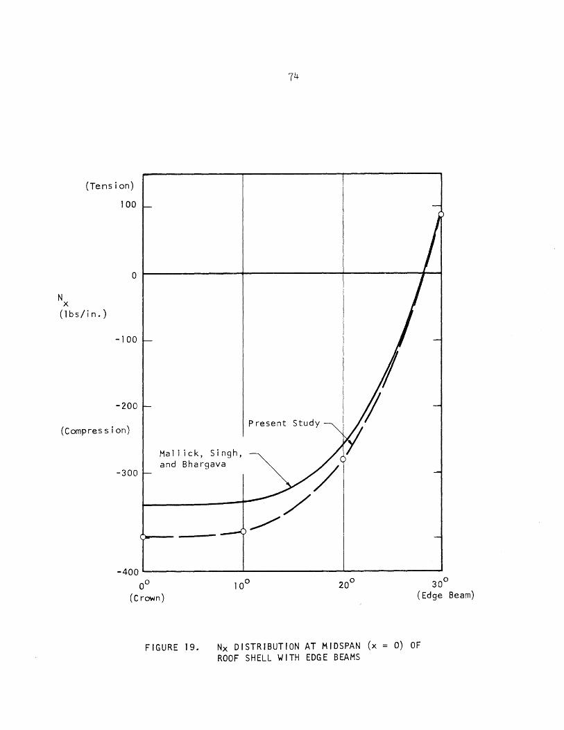
N x

(Tens ion)

100

74

o r-------------~--------------~----------~~

(lbs/in.)

-100

-200

(Compres 5 ion)

-300

Ha 1 1 i c k , Sin g h , and Bhargava

Present Study

-400----------------~--------------~------------~

0° (Crown)

FIGURE 19.

30° (Edge Beam)

Nx DISTRIBUTION AT MIDSPAN (x 0) OF ROOF SHELL WITH EDGE BEAMS

N xy

75

Oo---------------~--------------~------------~

-100

Mall ick, Singh and Bhargava

(lbs/in.) Present Study

\ -200 \

\

-300 ~----------------~------------~--------------~ 0°

(Crown)

FIGURE 20. Nxy DISTRIBUTION AT SUPPORT (x ROOF SHELL WITH EDGE BEAMS

30° (Edge Beam)

25 ft) OF

300 r--------------,---------------r---------------

(Tens ion on

( Ins ide)

M Y

200

( i n-1 b 5/ in. )

100

Or--------------+~~----------+-------------~

-100

-200

(Tens ion on

outside)

Present Study

Mall ick, Singh, and Bhargava

-300----------------~--------------~-------------J 30°

(Edge Beam) 0°

(Crown)

FIGURE 21. My DISTRIBUTION AT MIDSPAN (x = 0) OF ROOF SHELL WITH EDGE BEAMS

E = 333.3 psf \J = 0.0 t = 0.03 ft

JAS

= JHS

= 1.0 x 10- 5 ft 4

Gravity Load: 1 psf

Stiffened Rec tangu la r Cutout

Free Edge

77

Diaphragm Support

/

/

.03

Diaphragm Support

Free Edge

l r· 03 ft

f .09 ft

DETAIL AT EDGE OF CUTOUT (All Four Sides)

FIGURE 22. ROOF SHELL ON DIAPHRAGM SUPPORTS WITH STIFFENED RECTANGULAR CUTOUT

200 ~------------------~------------------~ (Tens ion)

Nx Present Study ---...

(1 bs/ft) 100

Pi ncke rt

o ~------------------~---.~~----------~

(Compress ion)

My

-100--------------------~--------------------

10° 20° (Stiffener)

FIGURE 23.

30° (Free Edge)

Nx DISTRIBUTION AT MIDSPAN (x = 0) FOR ROOF SHELL WITH STIFFENER AROUND CUTOUT

O~------------------~----------------~~

(ft-l bs/ft)

-.10 Pi nckert

(Tens ion on

Outside)-.20~------------------~------------------~ 100 20° 30°

(Stiffener) (Free Edge)

FIGURE 24. M DISTRIBUTION AT MIDSPAN (x = 0) FOR R60F SHELL WITH STIFFENER AROUND CUTOUT

79

C 0

FIGURE 25. CIRCULAR PLATE ELEMENT

80

A;'FENDIX A

ECCENTRIC STIFFENER-SHELL COMPATI3IL=~f

It is demonstrated in this appen.dix that the eccentric stiffener

element and the shell element remain f~lly compatible along their line of

intersection after deformation occurso This demonstration is acco~plished

by comparing the u displacements (displacement in the x-direction) of an

axial (longitudinal) stiffener and the corresponding displacements of the

shell at their common line or plane 0 A similar demonstration is possible for

v displacements using a hoop (circumferential) stringer 0

The u displacement at any point based on the shell reference surface

is

u u o

z w~ o 0

(A 01)

The corresponding expression for the displace~ent of a point based cn the

stringer ref-erenee -iline :.is

u u - Z w! st st st (Ao2)

In these equations) the subscript 0 refers to the scell and st to the

stiffenero The pr~e denotes differentiation with respect to xo It is to be

shown that the axial defo~ations at any point on the junction line of the

shell and stiffener are the same) regardless of which coordinate system is

used. Therefore) it must be shewn that

(A.3)

81

The assumption has been made that the w displacement is the same throughout

the depth of the shell-stiffener combination. Therefore, Wo = wstc Also J

by geometry, Zst = zo'- C, where C is the eccentricity of the stiffener. Now,

Eq. (A c 3) can be transformed ~

W.! o

-Ll - U o st

C (A.4)

The deformation functions used must now be considered. These are:

where uo1J u b2' ... ,

u o

w o

w

coordina tes) , and Hl ,

polynomials (see Fig.

01' ... , ustl '

H2, H3

, and H4

3) . Equations

(A.5)

u th are constants (generalized s ,

are the four Hermitian interpolation

(4-.9) and (4.10) relate the shell

coordinate system to the stiffener coordinate syste~. These are rearranged

and evaluated at the stiffenei: element and points in terms of the Hermitian

interpola t·ion polynocials to yield ~

U 1.:. ,., w stl :"1 v c3

u ~~ - C w 04 st2 02

{- -t wo4}

(A 06)

C 6 6 4 u

st3 u

03 - -w + L 2 -w 02 - - w

L2 01 L 03

r. {+ 6 6 2 + t wo4} u

st4 u04 - Iv :;- W _ - -w +::;::-w J...J 01- T2 02 .lJ 03

J...J

82

where L is the element size in the x-direction. Substituting Eqs. (Ao5) and

(A.6) into Eq. (A.4), the equality to be demonstrated, one gets:

wolHi + w02H2 + W03H3 + W04H4 w03Hl + w04H2

{- 6 6 4 t wo4} H3 + L2 wol + -w - - W - (A.7) T 2 02 L 03 .l...J

+ {+ 6 6 2 + ~ w h} H, -w - -w + L w03 L2 01 L2 02 .l...J o. 4

The only way for Eq. (A.7) to be true is that it hold true for each

of the four independent variables: wol ' w02' w03 ' w04 0 Therefore, Eq. (A.7)

can be broken down into its four independent parts~

HI 6 6 - - H + """2 H) 1 L2 3 L 4-

H' . 6 H -

6 2 L2 3 2H4

L (A.8)

Hi Hl 4 2 - - H + L H4 3 L 3

HI H -2 4 L H3 + ~ Hh 4 2 L .

Equations (A.8) can be easily verified by applying the definitions of the

Hermitian interpolation polynomials found in Fig. 3. Therefore, .it has been

shown that the shell and eccentric axial stiffener system are compati.ble 0

APPENDIX B

STRA~N-DISPLACEMENT RELATIONSHIPS FOR THIN GYLINDRICAL S:sELLS

During a literature search J it was noted that there were many

different sets of strain-displacement relationships in use. While the

differences between them were not major, it was desirable to select the

most appropriate one. After some manipulation) most of these vario~s strain-

displacement relations can be expressed in the form~

E Y

E xy

dV W CJy + R

(l+A) R

(I+B) R

Values given to A and B by investigators are shown in Table Bol.

It can be shown by using the same two techn~ques employed by

Cantin (6) that any combination of A and B will give a set of strain-

(Bol)

displacement relationships that are strain-free for all rigid body motions.

This, ~owever, still leaves the question as to which values of A and B should

be selected.

Vlasov (37) argues that the table of differential operators of the

equilibrium equations must be symmetric about its main diagonal in order to

satisfy the reciprocal theorem. He demonstrates that his set of strain-

displacement relationships satisfies this criterion. He does not demonstrate,

however, that his set is ~nique in any way. It will be demonstrated in the

84

remainder of this appendix that there is a unique set of values for A and B

that make the table of operators symmetrical, and that these are indeed the

same as those arrived at by Nlasov (37).

For the general case, the table of differential operators is shown

on Table B.2. If this table is to be symmetric; the following equations must

be satisfied~

3B + 1 -1 - B

-1 - 4B ~l

l+A 0 (B.2)

-1 - A = 0

-5 + V - 2vA - 4B(1-v) -3 + V

They can only be satisfied if and only if A = -1 and B = -~. Therefore, the

equations given in Section 3.2 for the strain-displacement relationships are

felt to be the most appropriate for use in this analysis.

AUTHOR A B Love (21 0 0

Timoshenko (34) 0 0

Novozh i lov ( 6) 0 0

Novozh i lov (25) -1 1 2

Langhaa r (20) -1 1 2

Vlasov (37) -1 1 2

Flugge ( 13) -1 1 - "2

Naghdi (6) 1 0

Sanders (30) 0 1 4

TABLE 8-1. VALUES OF A AND B USED BY VARIOUS AUTHORS

2

3

u v

~ 2 d 2 ( 1 -v) t

2 .- + - - (1 - -- B) ox2 oy2 2 12R2

o f 1 +v t 2

(1 -v) } d xoy L-2- + --2 -2-· (-I-B) 12R

{ 2 o 1 ~\) t J -\I ~ -2-+-2 ("2) (3B+l)}

12R

62 02 (1)( 2 ~ + -2 ;v 1 + ~(4+3B)) Oy Ox 12R

+ ,,3_(1;\J) (1- 4Bl}]

1 r'Va t2

{ "03

R Lax - 12 0 x3

1 r- a {t2 } R Ldy I - ----z (I + A)

12R

03 {2 + --3 ~ 2 (- 1 - A)}

Oy

+ + (~){-5+V-2VA-I+B (I-v l}] Ox 0 y

NOTE: 2 2 'V 'V

?I .~ d L~ 0 LI-~+2 +----r ..,.4 - 2 2 ~q. Clx dx oy uy

w

1. [,JoO _ R OX

t 2

{ 0 3 d 3

(1 -v)} l 12 dx 3 - "OYiJy -2- J

t [ 0 t 2

03

{ 1 -}] R ~ + 12 2 02( -3+v) ox oy

2 2 2 2 [ t \)(\

'V 'V + 2 12 -2(-A-l) R -'Ix

2 2 - ] t ~ ~ (1 -A) + 1 - ~ A + 12 ~ 2 12R oy

TABLE B-2. DIFFERENTIAL OPERATORS

Load Terms

l_v 2

ft PI

1 _\12 ~P2

1 _v 2

- -E-t- P3

~