a Fermi National Accelerator Laboratory

FN-505 [SSC-N-5941

Analytic Expressions for the Smear Due to Nonlinear Multipoles

Nikolitsa Merminga Fermi National Accelerator Laboratory

P.O. Box 500, Batavia, Illinois

King-Yuen Ng SSC Central Design Group

c/o Lawrence Berkeley Laboratory 90/4040 Berkeley, California 94720

and Fermi National Accelerator Laboratory

P.O. Box 500, Batavia, Illinois

February 1989

a Operated by Unlversitles Research Association, Inc., under contract with the United States Department of Energy

FN-505

SSC-N-594

ANALYTIC EXPRESSIONS FOR THE SMEAR DUE TO NONLINEAR MULTIPOLES

Nikolitsa Merminga

Fermi National Accelerator Laboratory’ Batavia, IL 60510

and

King-Yom Ng

SSC Central Design Group’

c/o Lawrence Berkeley Laboratory 90/4040, Berkeley, CA 94720

and

Fermi National Accelerator Laboratory’ Batavia, IL 60510

(February 1989)

*Operated by the Universities Research Association Inc., under contract with the U.S. Department

of Energy.

I. INTRODUCTION

The linear aperture is a region around the axis of the magnets in a collider ring

where the particle motion is sufficiently linear. Such a region is necessary to allow for

stable and efficient beam operations. The linear aperture is also regarded as the prime

requirement in choosing the inner diameter of the magnet coil package. A smaller coil

size implies a lower magnet cost.

For truly linear motion, the particle trajectory in the phase space at a certain

location along the ring maps out a perfect ellipse which is an invariant. In the pres-

ence of nonlinearities, however, the trajectory fluctuates about the ellipse from turn to

turn. The rms fractional value of this fluctuation is called the single particle smear.

Based on past accelerator experience, 11Jl the linear aperture of the SSC is defined

quantitativelyI as the region within which the smear is less than 6.4% and the on-

momentum tune shift with amplitude is less than 0.005.

In experiment E778 performed at the Fermilab Tevatron, the multiparticle smear

was measured[4] f or various sextupole excitation currents. The results appeared to agree

excellently with multiparticle simulations. Single-particle tracking was then performed

with exactly the same machine inputs as the multiparticle simulations to convert the

observed smear of the beam to that of a single particle. It would be very useful that

the single particle smear can be computed directly from the lattice. This is because

such computation can tell us immediately whether the multipole errors in a particular

sample dipole and the particular distributions of correction multipoles arc acceptable

or not without resorting to extensive tracking. Such possible screening procedure for

random multipole field errors has been attempted by Peggs, Furman, and Chao.1’1

In this paper, analytical formula: are presented for the computation of smear due

to both field errors and correction multipole insertions. Specifically the one- and two-

degree-of-freedom expressions for the smear due to sextupoles and octupoles are given

first. In this particular case we show that the smear has a very simple expression in

terms of the norms of Collins’ distortion functions. 1’1 It will be shown later that this is

not the case upon the addition of higher multipole terms. The reason is that there is

in general more than one multipole contributing to the same harmonic component and

1

hence their contribution is not separable. Next, a generalized formula for the horizontal

smear due to all multipoles is derived. Since horizontal and vertical coupling is usually

minimized during actual machine operations, the formula for horizontal smear should

be adequate for all practical purposes. In these derivations the periodic structure of

the multipoles in the ring is taken into account. Analytic expressions for the smear

have also been derived by Forest L71 but in the complicated hard-to-follow Lie algebra

language. Our analytic expressions are simple.

Finally, a number of applications demonstrate the usefulness of these calculations.

In particular, the smear as calculated in this formalism, is compared with the smear ex-

tracted from experimental observations during E778, for a variety of conditions. Results

from tracking calculations are also presented and comparisons are made. Moreover, the

smear introduced in the Tevatron due to random and systematic multipole errors in

the dipole magnets is calculated. The same calculation is repeated for the SSC ring.

Furthermore, the calculation of the smear in the SSC is done after the insertion of

correction elements for random multipole errors. The lumped correction scheme chosen

for this calculation is due to Neuffer. [81 Various cases are examined and comparisons

with tracking results from Sun and Talman, 1’1 and other analytical calculations due to

Forest and Peterson[l’l are presented.

II. SMEAR DUE TO NORMAL SEXTUPOLES

One-Degree-of-Freedom Calculation

Consider the situation of having only sextupoles in the ring. For first order pertur-

bation, the distortion of the horizontal particle amplitude P, at phase advance I& is

given byIll

6&(h) = d:{[A1(&)sinrp, - &(&)cosip,l

+ [Ad&) sin 31~~ - &(h) ~0s 310~1) , (2.1)

where ~0, is the instantaneous betatron phase such that

I = dzcosp, (2.2)

2

and

2’ = -sl, sin ppz,

and the phase advance G5 is defined by

44s) = J,’ &.

(2.3)

(2.4)

Here Br, Al, Bar and A3 are the Collins’ distortion functions defined by

(2.5)

The summations over k above, are over each sextupole located at the ‘modified’ phase

advance Q,&, which is related to the usual Floquet phase g,k by

4 rk

if &k 2 & , *,:, =

*)B!? t 2?rv, if $.k < 6 , (2.6)

depending on whether it is upstream or downstream of the observation point &.

The horizontal amplitude A, has been normalized so t,hat it is a constant of motion

(or the Courant-Snyder ellipse is a circle) for the perfectly linear machine. It is related

to the horizontal emittance t, by

TdZ. 5

t =K’ (2.7)

where PO is a reference length specially introduced so that the amplitude A retains the

dimension of length. The normalized vertical amplitude R, has been set to zero.

3

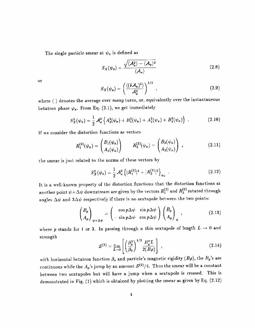
The single particle smear at & is defined as

(2.8)

(2.9) where ( ) denotes the average over many turns, or, equivalently over the instantaneous

betatron phase (P=. From Eq. (2.1), we get immediately

si(+z) = ; d: { Ai(+=) + %($k) + A:(&) + B:&)}

If me consider the distortion functions as vectors

the smear is just related to the norms of these vectors by

s;(h) = ; A: { lRy)12 + IR~)/*}$=

(2.10)

(2.12)

It is a well-known property of the distortion functions that the distortion functions at

another point $+A$ downstream are given by the vectors Ry) and Rc) rotated through

angles hli, and 3A$ respectively if there is no sextupole between the two points:

(:),.,+ = (-:;::z: ::::“,::) (::), ’ (2.13)

where p stands for 1 or 3. In passing through a thin sextupole of length L + 0 and

strength

(2.14)

with horizontal betatron function pz and particle’s magnetic rigidity (Bp), the En’s are

continuous while the A,‘s jump by an amount St21/4. Thus the smear will be a constant

between two sextupoles but will have a jump when a sextupole is crossed. This is

demonstrated in Fig. (1) which is obtained by plotting the smear as given by Eq. (2.12)

4

Smear around the machine

8-

7-

I- 6-

- v 19.38 = 5 -1s = 10 Amps

- 10kV

4 I ! I I I I I I I I I I I I I I_ 0 5 10 15

Phase advance / 2n

Figure 1: Smear versus phase advance, around the machine, as predicted from pertur.

bation calculation.

as a function of the phase advance around the Tevatron during the performance of

E778. Sixteen sextupoles clustered in two groups of eight located at phase advances of

approximately 4.5 x 27 and 14.5 x 2x cause these jumps in the smear. In the special

situation of having only one sextupole in the ring, the smear becomes a constant of

motion.

Further insight can be obtained from the expression (2.12) for the smear in terms of

phases and sextupole strengths. The definition of the distortion functions (2.5) implies

or

Similarly,

that

B:(+=) + A:(k) = 64si;z =~ c S!“)$) cos($:, - &,,) , = k,k’

(2.15)

W(4 z )I = 81 sinl~u.1 1~s!2)c’*‘k 1

(2.17)

Therefore, if we want the horizontal smear to vanish at a particular point 4, what we

need is to arrange the sextupoles so that

$-.$)e’“; = 0 and ~S!‘)e+k = 0 (2.18)

If the sextupoles are random errors in dipoles say, then we have

R$@ t Rr)’ = ; .& 2

+ sin2;Tv *) p? i

where (SF)‘) is the variance of the sextupole error at location k. Note that for purely

random errors, the smear is identically the same at every point around the ring. Thus,

these errors cannot be corrected in any way. However, in a machine like the Tevatron,

every dipole has been measured. In other words, all the “random errors” at the dipoles

are actually known. As a result, they can be corrected using correctors. In Chapter

V we present examples of how one can calculate the smear due to random sextupole

errors in realistic cases.

Two-Degree-of-Freedom Calculation

In two degrees of freedom the distortion of the horizontal amplitude R, at phase

advance &, to first order in the sextupole strength, is given by[“]

6A, = dz[(A, sin (p2 - B1 cos vp.) + (As sin 39, - Bs cos 39.)]

-dz(2(Asinvp, - Bcos p2) + (A.sinp+ - B, cos q+)

- (Adsin+ - Bdcosrp-)] (2.20)

The distortion of the vertical amplitude 4 is given by

6% = -2d&[(A, sin p+ - B. cos rp+) f (Ad sin ‘p- - Bd cos p-)] (2.21)

The distortion functions A,, B,, AZ, 83 are given by Eq. (2.5) while B., A., I&, Ad,

B, i? are given by

&(ljt+) = 2si;hv ~ $+ - Tv+) >

A($+)= .l C .$’ --in($>,-ti+-rv+), 2smirv+ k 4

.I$) Bd($- 1 = 2 si;,,- c -

k 4 cos ($‘, - q!- - 7x) ,

$1 Ad(h) = 2siJnv_ c 4 sin (dtk ~ $- - TV-) ,

k

B(h) = 2 si;nv

$’

c 4 cm (a? - dJz - 4 1 = k

41CII) = 2si,l,,

$1

I- 4 sin (dk - $3 - w) , 5 k

(2.22)

where $i = 2$, & 4, and vi = 2v, l u,. Again here r+!& and #,, are the modified

phase advances defined in Eq. (2.6). Th e sextupole strength L?(*) is defined by

(2.23)

In two degrees of freedom one can define three different kinds of smear:

(2.24)

and

Sxu = ((we”)“* )

where ( ) denotes again the average over the instantaneous betatron phases p2 and lpy.

Using Eqs. (2.20) and (2.21) one can express the three smears in terms of the Collins’

distortion functions as follows

S;, = ; ..43A; + B: + A; + Bj)

+ ; $[A: + B,2 + AZ, + Bj + 4(2 + i?)] - 2d;(A,A + L&B) , (2.27)

S&J = 2d;;A; + B,Z $ A; + B,j) (2.28)

S&J = d;(A: + B,Z - A; - Bj) . (2.29)

If we consider the distortion functions as vectors, similarly to the one-degree-of-freedom

case,

&(4+)= Rd($-)= (2.30)

the three smears are expressed in terms of the norms of these vectors as follows

Six = ; A: { lR?+ lRa12}+e t ; $ {IR,~‘+~Rd~‘t41fila}~~-2~(R~,R), (2.31)

and

s$, = 2d: { lR,12 + iRdl’}+= > (2.32)

S;, = d; { IRS!* - lR#}+=

In the above (RI, R) denotes the inner product of the vectors RI and R.

(2.33)

8

From Eq. (2.22) we have

A; + B,2 = (2.34)

OC

lRa’ = 81 sinl?rv+l k /pW:.l .

Similarly

/C $%iKkl )

k

,R, = 8, ,;,‘,,, 1pW.~ I

and

(RI,@ = ’ ~@‘.~)S~?.~)COS(& - $Lkr). 64 sin’ xv= k,k,

Hence (2.27), (2.28) and (2.29) become

and

(2.35)

(2.36)

(2.37)

(2.38)

s+;$ 1

1 c,, Sf)& y + 1 c,. spew 12

sin* 7rvs sin’ 3r;u, I 1 4

+ 5 64d; -i

lCkpe+;kIZ + ICkpey + 4~y-p&qZ

sin’ 7rv, sin’ xv- sin’ 7rv,

AZ, 1 c s!“‘s,y cos ($& - &‘) , 32 sin’ TV, k,ks

(2.39)

.a: SFT = 32

1 Ck @@kh 12

sin’ 7rv+ (2.40)

Jq 1 -&p&q s;, = s4 1

, -yk p,hc* 12 - sin’ XV+ 1 sin’xu- .

(2.41)

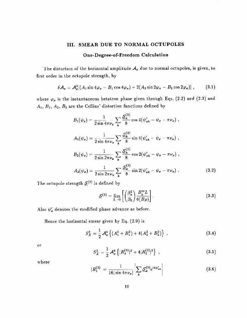
III. SMEAR DUE TO NORMAL OCTUPOLES

One-Degree-of-Freedom Calculation

The distortion of the horizontal amplitude & due to normal octupoles, is given, to

first order in the octupole strength, by

S& = d;? [( A, sin 4~~ - B, cos 440~) + 2( A2 sin 2+9, - Bz cos 21p,)] , (3.1)

where (F= is the instantaneous betatron phase given through Eqs. (2.2) and (2.3) and

A,, BI, AZ, Bz are the Collins’ distortion functions defined by

B1(42) = 2 sin:Tv s(3)

c * cos 4(9$, - $b - 7%) , = L

Al(A) = 2sin;nv g”’

C - = k

8 Sin4(& - A - nvz) ,

BZ(&) = 2sin;Tu 1% cos 2(2c1L - lity - xvz) , = k AZ(A) = 2sin;;rv sy I-

= k 8 sin2($:, - +, - TV=)

The octupole strength SC31 is defined by

‘$3) = 1’ - E[(g)i&

Also $k denotes the modified phase advance as before.

Hence the horizontal smear given by Eq. (2.9) is

S:, = ; d: {(A; + B:) + 4(A; t B;)} ,

or

where

‘i = ;A: { jRj3)/2 + 41Rp)/Z} ,

(3.2)

(3.3)

(3.4)

(3.5)

(3.6)

10

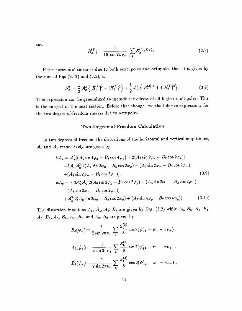
and

lR(23’1 = 16, si:2?ru.l ipW*:*~

If the horizontal smear is due to both sextupoles and octupoles then it is given by

the sum of Eqs (2.12) and (3.5), or

s; = ; -4: { lR(,2)1’ t IRr)(‘} + ; dz { ,Ry)la + 41R(Z3)12}, (3.8)

This expression can be generalized to include the effects of all higher multipoles. This

is the subject of the next section. Before that though, we shall derive expressions for

the two-degree-of-freedom smears due to octupoles.

Two-Degree-of-J?reedom Calculation

In two degrees of freedom the distortions of the horizontal and vertical amplitudes,

& and d,, respectively, are given by

6A, = dz[(A1sin4ip, - B, cos 497,) $2(Az sin 2+9, - Bz cos 2~,)]

-3Adt[2(AS sin 2rp, - BS cos 2~~) + (AZ sin 29+ - B3 cos 250+)

+(A4 sin2ip- - Bq cos2ip-)], (3.9) SR, = -3d$k,,[2(AG sin 2~~ - Bg cos 2rp,) + (AS sin 2$~+ - & cos 2Q+)

-(Ad sin 2~~ - Bq cos 2+)]

+&,[2(A8 sin 2rp, - & cos 2Q,) t (AT sin 4rp, ~ B, cos 4Q,)] (3.10)

The distortion functions A,, &, Al, Bz are given by Eqs. (3.2) while As, &, Al, B4,

As, Es, As, Be, AT, B7, and As, Es are given by

fL($+) = COS2(1c>k - 4+ - rut) 9

&(4+) = ’ SF’

C s sin 2(+& - $J+ ~ TV+) , 2sm2rrv+ k

SW h(k) = 2sin;T1/_ 1 +cos2(L - TL - mm) ,

k

11

A4(2CI-) = 2 sinlZliv- C Sp - sin 2($,‘, - +- - ~TL) ,

A. 8

Bdd4 = 2sin;x” Sf ’

c - cos 2(4-L - ?L - 4 1 2 k

8

AdlC1=) = 2 sininv SF’

c 8 sin 2(& - A - xv=) , = k

w&J = 2sin;Tu Sf ’

c - 8 cm 2(7&k - A - rug) , Y k

Ad&) = 2siniTv Sf)

C s sin2(& - +, - T,) , Y k

ads,) = 2 sin;?;v $4

c 7 cm 4(9&k - 4% - qJ 1 I/ k

AT(&) = 2 &,, $3

c - II k 8 sin4(& - 11, ~ w) ,

w&J = 2sin;T” c $3

Y k 8 cos 2(&k - lil, - ql) i $’

AS(&)= ’ ~~sin2(&-&-~vy). 2sm27rv, k

(3.11)

Here v* = uz zk vy and $+ = $. zk $,,. The octupole strengths S@) and .!?@I are defined

by

s~~‘+i#$$)g$], (3.12)

and

s;(‘yi#$&. (3.13)

Again $I’ denotes the modified phase advance. Then the three different smears given

by (2.24), (2.25) and (2.26) are

s;, = ;d:[(A:tB:) + 4(A;+B;)] + ;d;[4(A;+B,2) t (A;tB;) + (A;+Bf)]

- 12dfd;[AzAstBzBs] , (3.14)

12

S:, = ;d:[4(A:+B;) i (A;tB,2) t (A;tBj)] t ;d;[4(A;tB,2) + (A;+B;)]

- 12d~d;[&AstB&] , (3.15)

and

S;, = ;d;d;[(A;+B;) - (A;+B,Z)]. (3.16)

We define, as before, the vectors RF), Rp), Rp), Rp), Rp) and Rf) such that

Then Six, S& and S’& become

s;, = ; A: { lR(,3)12 t 4lR(23)/‘} + id: {4lR(,3)1* + /Ry)l* + lRy)lZ}

- 12d:d;(Rp), Rp)) , (3.18)

Si,y = id: {41Rf’/’ t IRp)l’ t IRf)l’} + :,4: {4iRf)12 + iRp)I’}

- 12d:d;(Rr), Rr)) (3.19)

and

S;-, = ;d:d; { IRf)12 - lR~)i”} . (3.20)

Using the definition of the distortion functions we arrive at

lR;)/ = (3.21)

IRp)l = (3.22)

JR?‘1 = (3.23)

lRf)l = (3.24)

13

Hence the three smears are given by

1 )Yk &)&* 12 t

41 c,, &‘% 12

sin’ 4Kv= sin’ 27rv,

41 Ck Sye’q~ + / Ck sfwq + / &, Sk P)ei24’i/*

sin’ 2w, sin’ 2w+ sin* 2kv-

and

-12dx 1 c spsp cos 2(&, - ?&,#) 256 sin’ 2xv, k,k,

so, = 9 A;& I& sf)&~. I2 1 Ck sf)eizl/i’l. I2 - 2 256 sin* 2iw+ sin’ 2rv-

IV. HORIZONTAL SMEAR DUE TO ALL MULTIPOLES

(3.25)

(3.26)

(3.27)

(3.28)

(3.29)

In this section, we want to derive a formula for the horizontal smear with the contri-

butions from all higher multipoles without resorting to the use of distortion functions.

The irrotational magnetic flux density inside the beam pipe can be written in general

as

By t iB, = Bo '&b, t &)(a: t iy)" , (4.1) n=1

14

where b,, and a, are the normal and skew multipole coefficients, respectively, of order

2(n + 1). For example, b = 1 an&l n

n!Bo I%:- (4.2)

In above, the vertical bending magnetic flux density B. as well as the field gradients

of the focusing F and D quads have been excluded. Thus, Eq. (4.1) contains the

contributions of all field errors as well as other inserted correction multipoles only. Since

we are concerned with the isolated horizontal phase space only, Eq. (4.1) simplifies to

B, = Bo 5 b,d’ n=l

(4.3)

In terms of action-angle variables I and a, the motion of a beam particle is described

by the Hamiltonian[12~13]

H=vI+AH, (4.4)

where

AH=n$l$+ qL +=+I

n+l’

The derivation is given in the Appendix. The subscript L will be suppressed below for

convenience. In the Hamiltonian, the independent variable is 0 = s/R, where s is the

distance measured along the ideal designed closed orbit and R is the average radius of

that orbit. The normalized horizontal displacement is given by

2: = dcos[Q(B) + a] , (4.6)

where the normalized amplitude is

A = (21&J1” , (4.7)

and the function

is periodic in 8.

Q(e) = N4 - A (4.8)

With the help of the trigonometric identities

CosZm+l+ = L+ m 2mlt1 4 1 cos(2m-2etl)d, k0

15

COPip = & m 2m cos2(m-44

I( 1 f=O e

6,+1 ’ (4.9)

for m = 1, 2, 3, . , Eq. (4.5), the higher multipole dependent part and field error

part of the Hamiltonian, can be rewritten as

(;)m& (2;) cosz(+:)!Q+a)

Ah+’

2y2mt 1) cos(2m-2e+l)(Q+a). (4.10)

The change of I with respect to 6’ is

dI

z= -y = zlz ‘$iym’ ( $md~~~~~e) sin2(m-e)(Q+a)

m+fd2”+1(2m-2~~1)

2292m+1) sin(2m-2etl)(Q+a) . (4.11)

Because we are interested in the first-order deviation from the linear amplitude

6d, or the first-order deviation from the linear action &I, on the right-hand side of

Eq. (4.10), I can be considered o-independent and a can be obtained from the equation

da i3H

zf=al”“’ (4.12)

0*

a(e) = !A t $9 , (4.13)

where ‘p is an initial phase. Then, the integration of Eq. (4.10) can be performed easily.

Noting that Q(8) is periodic in 9, we obtain

16

P x PO (-1

m+~dZm+1(2m-2e+1) 2mfl

22m+'(2mt 1) ( 1 e cos(2m-2etl)(Q+a-?rv). (4.14)

Taking the thin lens approximation and defining the multipole of lengths L + 0 and

strengths as

Sf”-‘) = Ei [ ‘$‘T (L)oL] k for the 4m-th multipole

for the (4mt2)-th multipole , (4.15)

Eq. (4.13) can be rewritten as

(4.16)

where the summation over k is for all the multipoles around the ring and we have used

$$, the modified phase location of the multipole as defined in Eq. (2.6).

We notice from Eq. (4.16) that multipoles of different orders can have the same

cosine dependence and they will be mixed. Thus, it will be better to sum up p = m-e

instead. Then, Eq. (4.15) becomes

6d A

_ _ g-c .g “@“-24?“-‘)fP’) cos2p($;~16+T”+p)

p=l k m=p sin 2pirv

(4.17)

with fizm-l) and fczm) defined as P

for the 4m-th multipoles

fW = 2pSl P 22”+‘(2m+l)

for the (4mt2)-th multipoles (4.18)

17

The ’ in the summation implies that m = 0 is excluded. Finally, an average over the

initial phase ‘p is performed to obtain the smear S defined in Eq. (2.9). We get

s2 = ; 2 c 2 d*m-2~;;~~m-‘~ e izp+; 2

p=l k m=p

2

(4.19)

If the higher multipoles discussed here are all random in nature, the square of the

smear can be simplified to

,+2fj2”-1) ’

sin 2pw 1 (4.20)

where (S, (2m-1) “) and (So”‘“) are the variances of the 4m-th and (4772 + 2).th random

multipole errors respectively.

18

V. APPLICATIONS

1. Beam Dynamics Experiment E778

Experiment E778 performed in the Fermilab Tevatron, studied the nonlinear dynam-

ics of transverse particle oscillations. U41 Nonlinearities were introduced in the Tevatron

by sixteen special sextupoles. A low emittance proton beam was injected into the Teva-

tron. The sextupoles were then ramped up to their final setting. The injection kicker

was used to induce a coherent bet&on oscillation. The centroid beam position was

recorded in each of two adjacent beam position monitors. From this information the

phase space motion could be tracked[“] and the smear could be extracted.

The smear was one of the parameters used to characterize deviation from linear

behavior. Measurements were repeated over a wide range of conditions. Specifically,

measurements were made at various values of the sextupole excitation, the horizontal

tune, the kicker strength and the beam emittance. The sextupole excitation varied from

0 to 50 amperes in steps of 5 amperes. The horizontal tune assumed 5 different values

from 19.38 to 19.42 in steps of Ill while the vertical tune was set to 19.46. The kicker

strength was 5, 8 and 10 kilovolts corresponding to 2.25, 3.8 and 4.5 mm in amplitude.

Finally, measurements were taken at two different ranges of the horizontal emittance.

At the low range the emittance varied from 1.5~ to 3.7x mm-mrad while at the high

range it was between 7.8~ and 10.9r mm-mrad.

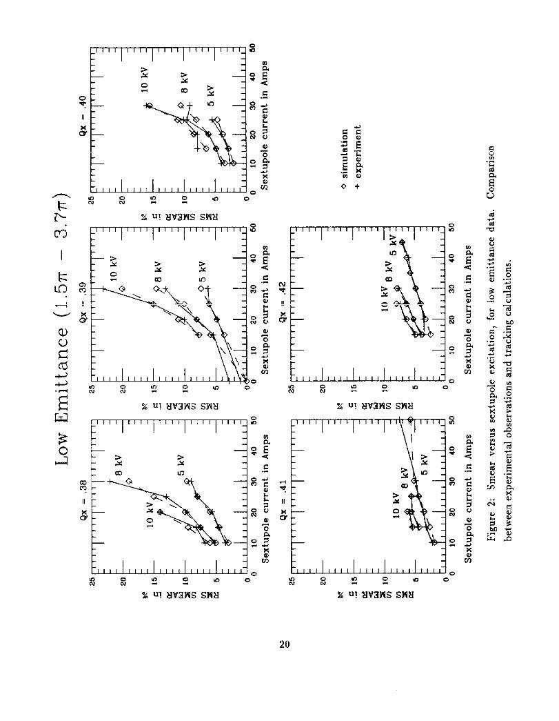
Single and multiparticle tracking calculations were done to simulate the above ex-

perimental conditions and the smear was extracted from these calculations. It was then

compared with the smear extracted from the experimental data. In order to demon-

strate the agreement between experimental and simulated data for the smear we display

Fig. (2). Here the smear is plotted against the sextupole excitation, for five tune values

(19.38 to 19.42). The three curves in each of the five plots correspond to the three dif-

ferent kicker strengths. The dashed lines represent prediction from tracking calculations

while the solid lines correspond to the experimental data.

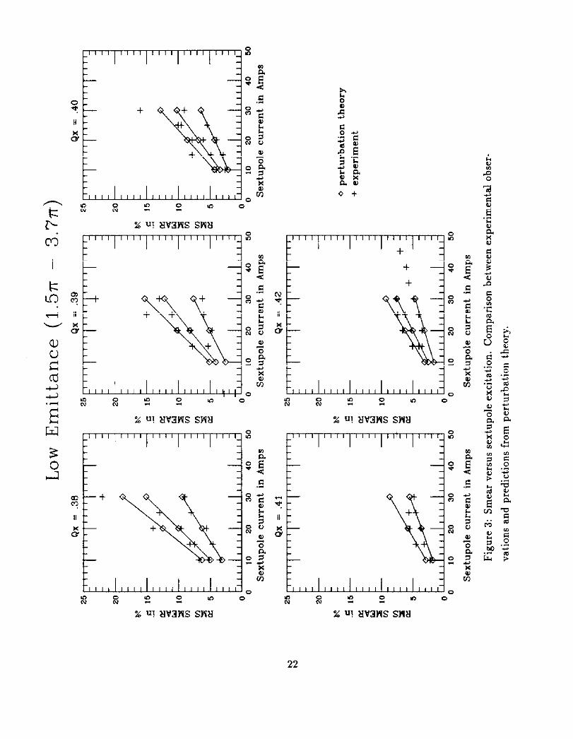
Next the smear due to the sixteen special sextupoles was calculated using Eq. (2.12)

and compared with both single particle tracking calculations and experimental data.

Fig. (3) displays the comparison between the prediction of perturbation theory (solid

19

::

s;

.E wz

2 ,szi

0 z

“3

” aw 10 0 m 0

4 .z 2 i .5 Sk ‘Z 3 0 +

% U! W3RS SAX

c”

L \ 20

20

line) and experimental data for a low emittance beam (crosses). Again the three differ-

ent lines in each of the five plots correspond to 5, 8 and 10 kV of the kicker strength.

The agreement between observation and prediction is very good especially in the low

current - low kicker amplitude regime. The deterioration of the agreement observed at

higher currents and kick amplitudes is due to the fact that nonlinearities are too strong

to be handled perturbatively. Finally, Fig. (4) displays the comparison between per-

turbative calculations and single particle tracking predictions. The previous comments

can presumably explain any disagreement between these two methods of predicting the

smear.

2. Smear Due to Multipole Errors in the Tevatron Dipoles

2a. Random Errors

Each one of the 776 Tevatron dipoles is characterized by a set of harmonic coefficients

(an, b,): the normal and skew multipole coefficients of order 2(n + 1). The mean value

of each multipole component calculated over the number of dipoles constitutes the so-

called syst,ematic error while the rms value constitutes the random error of the particular

multipole. Table I displays the values of both the systematic and random multipole

errors for the Tevatron dipoles, 1161 up to the 14.pole. These values correspond to a

magnetic field of 4000 amperes. The unit,s of b, are 10e4 cm-“, and the values are 1O-4

of the integrated dipole field at 1 cm radius. In the following we shall use Eq. (4.20)

to calculate the smear due to all higher multipoles of the Tevatron dipoles, assuming

they are random in nature. Since the highest multipole with a non-zero coefficient is

the 14.pole (n = 6), Eq. (4.20) becomes

&“-2f(2”-I) ’ 776 =

sin 2prv 1 k=l 1 2 776 (5.1)

where the prime in the first sum implies that the m = 1 term is excluded (since b, is

the normal quadrupole field) Th’l N 1 e in the second sum the prime implies that the m = 0

21

I L 4 5! k u3$ .+ II VX m

Ii-

Q, z 2 -4 .3 2 :: rr

+

A

\

z + +

:: +

0

0 II) 0 Ic) 0

z E <

Fh E <

0 +

::

s

2 w I/ s Ei

D

0 a g 2 5: 0 0

% “! &x3AS SW8 I ,,I I I1 I I I I I ,,#I, ,,,I ::

s

?I a II - 6- ::

k E:

III! ,,,I IIII III, IIll.o kc i-2 z? 0 n 0

x “! tlv3m snll

& 9

E $ -z TJ .c

e 8

2 22 E 2 ; 25 016 z E 5 $2

f; ‘2 .- 5 rt *z ‘g 2

u 0 2

z G 2” s E % 4

E. 22 E < z .o

.c Y 5

-s ; z

5 Ea

5 mv

0 - 9 0) i! 2 z &.+ 2 I% Is

i;; $

rz

22

L’ I I I, I, I I, I I II, I I I ‘AS

2 2

% U! siv3ws SW8 % U! siv3ws SW8 IIII III, /II, ,I,, s IIII III, /II, III, s

2 2 2

ul ul

[\j ;\i

E z-2

Q, ? Q, ? + + .e

-2 ; II ; II EE .3 &J .3 &J

z z 2 ‘y ‘y

2 2 2: 2:

1 1

1, ‘I I I I I I I t I I I I I I I I I ,I

s s aJ aJ - : : III, I,,, I,,, I,,,

-$)gj 2 0 ul -$)gj 2 0 ul o” o”

c: c: % 4 w3ws SAtl % 4 w3ws SAtl

5 I/ + 2

~ x rz

0 E Lo 2 UT 0

III1 III/ /II, III, s !z E

zq .c

5

wi

% I/ + ::I2

2 2 2

0; ‘i; rz

III, III, II,, I,,, 0 E Lo 2 UT 0

% “1 W3AS SW&l % “! FlV3RS SW8

23

mu1t. co&. multipole System. errors Random errors

bl normal quadrupole 0.035 0.189

bz normal sextupo1e 0.1 0.484

bs normal octupole -0.014 0.047

ba normal decapole -0.014 0.032

b5 normal dodecapole - 0.003

bg normal fourteen-pole 0.020 0.002 J Table I: The constants b, are the systematic and random multipole errors in the Teva-

tron dipoles, expressed in units of 1O-4 cm?‘.

term is excluded (normal dipole field). Th e variance of the random multipole errors is

given by

since we chose PO = 8.

(St)‘) = ( ( $$L)k bL}’ (5.2)

For the Tevatron &,=4.4 Tesla, fl,,=lOO m, the dipole length is L = 6.12 m and

the magnetic rigidity Bp=10/3x900 Tesla-meters. The bl’s are given in Table I. This

calculation is done for a betatron amplitude of A=5 mm and for a tune of 19.23. Using

these parameters, the result for the smear in the Tevatron due to random errors in the

dipole magnets is

sTcv/ran = 1.04 %. (5.3)

This result is in agreement with observations done as part of the E778 experiment in

order to demonstrate the linearity of the Tevatron. 1171

24

2b. Systematic Errors

In order to calculate the smear due to the systematic errors in the Tevatron dipoles

we use Eq. (4.19). In the presence of the errors shown in Table I, Eq. (4.19) becomes

776 5 ,A&-2Sfm-‘)f(2m-1) 2

P

sin 2prv e iw;

(5.4)

776 K eiW 2 ’ [d2m-2S~m~‘)f~Zm-‘)] ~’ k-l m=p

$; [dZm-‘S~m)f~2”)] I’, (5.5)

where again the prime in the first and second sum means that m = 1 and m = 0

respectively are excluded.

If we consider a simplified Tevatron lattice which basically consists of a series of

FODO cells with the 776 dipoles equally spaced from each other around the machine

then the k-th dipole is at a location with phase advance

k y!l& = 2x x 19.23 x 776 (5.6)

for a tune of v=19.23. In this case one can easily perform the summations

(5.7)

and

as finite geometric progressions. Indeed

716 116 g @4; = 1 .+rk = ei4pn” - l ,

kl 1 - e-%r (5.9)

25

where 2KV

T=776 (5.10)

Also notice that the multipole strengths Sk are the same for all k and hence Eq. (5.5)

is simplified to

(5.11)

Using the values specified above, the result for the smear in the Tevatron due to sys-

tematic errors in the dipole magnets, is

S TCY,6ylt = o.fK% (5.12)

3. Smear Due to Multipole Errors in the SSC Dipoles Before and After

the Insertion of Correction Elements

The SSC dipoles are expected to have higher order multipole components which are

given in Table II below. The units of the harmonic coefficients b, are again 10e4 cm-“.

Though both random and systematic errors are present, the random errors are the

principal source of the smear. Hence the linear aperture of the SSC is dominated by

the random multipole components of the dipole magnets. Various correction schemes

have been devised to compensate for the random errors anticipated in the SSC. It

appearsi’] that the so-called three lumped correction scheme due to Neuffer [‘I is the

most effective one.

In the following we shall calculate the smear in the SSC due to random and/or

systematic errors in the dipoles using the formalism developed above. Then, we shall

introduce correction elements according to the three lumped correction scheme and

recalculate the smear for various situations. The purpose of this exercise is to demon-

strate that one can predict the smear of a fairly complicated lattice from analytical

methods without resorting to extensive tracking.

26

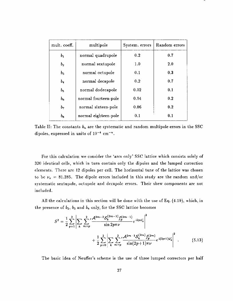
r mu1t. co&. multipole System. errors Random errors

bx normal quadrupole 0.2 0.7

bz normal sextupole 1.0 2.0

b3 normal octupole 0.1 0.3

bq normal decapole 0.2 0.7

bs normal dodecapole 0.02 0.1

bs normal fourteen-pole 0.04 0.2

b7 normal sixteen-pole 0.06 0.2

be normal eighteen-pole 0.1 0.1 J

Table II: The constants b, are the systematic and random multipole errors in the SSC

dipoles, expressed in units of 10m4 cm-“.

For this calculation we consider the ‘arcs only’ SSC lattice which consists solely of

320 identical cells, which in turn contain only the dipoles and the lumped correction

elements. There are 12 dipoles per cell. The horizontal tune of the lattice was chosen

to be v, = 81.285. The dipole errors included in this study are the random and/or

systematic sextupole, octupole and decapole errors. Their skew components are not

included.

All the calculations in this section will be done with the use of Eq. (4.19), which, in

the presence of bz, b3 and b4 only, for the SW lattice becomes

sz = ; & c 2 1 d2m-2S&)J?1’ e iw; ’

&%=I k m=p

(5.13)

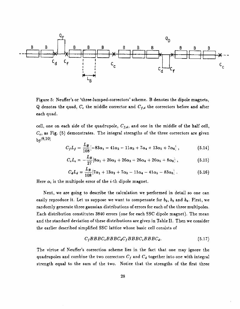
The basic idea of Neuffer’s scheme is the use of three lumped correctors per half

27

QD B B B B B B B B B B B

-- II L ” II II lvl I I II I.1 II I I 1” --

‘d ‘f I I 1 I : 1

Cc cc I I

“

Figure 5: Neuffer’s or ‘three-lumped-correctors’ scheme. B denotes the dipole magnets,

Q denotes the quad, C, the middle corrector and Cf,d the correctors before and after

each quad.

cell, one on each side of the quadrupole, Cf,d, and one in the middle of the half cell,

C,, as Fig. (5) demonstrates. The integral strengths of the three correctors are given by!8,101

CfLj = $[-83% - 41a2 - llas + 7a4 + 13as + 7&s] ,

C,L, = -$[8al+ 20~~ + 26a3+ 26~~ + 20~~ + 8as],

cd.& = ~[7u~t13a, + 7a3 - lhl - 41a5 - 83~1~1.

Here CZ; is the multipole error of the i-th dipole magnet.

(5.14)

(5.15)

(5.16)

Next, we are going to describe the calculation we performed in detail so one can

easily reproduce it. Let us suppose we want to compensate for bz, b3 and bd. First, we

randomly generate three gaussian distributions of errors for each of the three multipoles.

Each distribution constitutes 3840 errors (one for each SSC dipole magnet). The mean

and the standard deviation of these distributions are given in Table II. Then we consider

the earlier described simplified SSC lattice whose basic cell consists of

CfBBBC,BBBCdC,BBBC,BBBCd. (5.17)

The virtue of Neuffer’s correction scheme lies in the fact that one may ignore the

quadrupoles and combine the two correctors Cf and Cd together into one with integral

strength equal to the sum of the two. Notice that the strengths of the first three

28

correctors on the left of (5.17) are evaluated via the errors of the first six dipoles on the

left, while the other three correctors are evaluated via the errors of the six dipoles on

the right.

All these elements are considered as thin lenses. The correctors are located in the

middle of the interval between two successive dipoles. Thus there are four contributions

to the summation over k in Eq. (4.19). Specifically Eq. (5.13) becomes

640 640 640 + c s~~4&2P+')~:, + 1 spe"ww~, + c spe”w)~;,

k=l k=l kl II

2 . (5.18)

The strength of the Z-th multipole of the k-th dipole B, S& is given by

&J&9 p (l+‘w s(l) = ~ - Bk (Bp) p. poL ’ ( ) (5.19)

where a!’ is the error of the k-th dipole magnet. Similarly, the strength of the l-th

multipole of the k-th corrector Cj, is

(5.20)

where the subscript j stands for c, f and d. Also CJ, is given by Eq. (5.15), C,Lf is

given by Eq. (5.14) and CdLd is given by Eq. (5.16).

For the SSC lattice, the numerical values of the quantities defined above are: at

the energy of 20 TeV, B. is 6.6 Tesla. The dipole length Lg is 16.54 meters and

the maximum beta PO is 332.0 meters. In our calculation we assumed ,0 = po. The

amplitude was 5 mm.

29

/I

L ) Correct systematic bz, b3, bq. 0.0009 i O.O(

Systematic b2, bS, bq present. L I

Table III: Summary of the results of the analytic computation of the smear in the SSC,

Smear (%)

No correction. 7.09 i 2.53

bz, bs, b4 random and systematic present

No correction.

Random bz, bz, b4 present.

7.07 * 2.50

No correction.

Systematic b2, b3, b4 present.

0.39 * 0.00

Correct random and systematic b,, b,, b,. 0.43 * 0.22

Random and systematic b,, b,, b4 present.

Correct random b,, b,, bq. 0.43 & 0.22

Random b2, bS, b4 present. --

Correct random b2. 0.71 zt 0.25

Random b2, b3, b4 present.

1

with and without correction elements.

30

The results of our computation are summarized in Table III. The value of the smear

quoted is the average over 100 seeds and the standard deviation of the mean is quoted

as the uncertainty in the smear. It is worth pointing out that the value of the smear

fluctuates by a large amount depending on the seed one uses. It is important that this

fact is taken into account in the design of a real machine. If only the mean value of the

smear is used as a criterion for the determination of the linear aperture (apart from the

tuneshift), the good field region may turn out not to be sufficient for safe operation.

One should allow the smear to vary as much as say two standard deviations away from

the mean value, within the good field region.

The general conclusion is that the three lumped correction scheme is very effective

in compensating for the random errors. Moreover, this particular scheme is also very

effective in correcting for the systematic errors. This is expected, since it was initially

developed to correct for the systematic components, and only later it was shown that

it can be used to correct the random errors as well.

Another observation is that the horizontal smear (in the absence of skew multipoles)

is dominated by the sextupole component b2. The effects of b3 and bq are rather weak.

31

APPENDIX

The horizontal motion of a beam particle is described by the Hamiltonian[12*13]

HI = ; [P: + K&,X’] t ncl f!!& , where X is the horizontal displacement, P, is the canonical momentum, and K, rep-

resents the field gradient of the normal quads. The independent variable s is the

distance measured along some designed closed orbit. In below, the subscript z will be

suppressed. We perform a canonical transformation into the Floquet space using the

generation function 112 t 2

Gl(z,P;s) = - Px +P+- 4th '

where the differentiation in p’ is with respect to S. The Hamiltonian becomes 2 Hz = 4 Pop2 t po + n$, $$ 1 1

L!$L zTn+l

n+l’

(A.4

(A.3)

Here, the independent variable has been changed to B = s/R, where R is the average

radius of the designed closed orbit. Use has been made of the relation

2&Y-fY2 +4KPZ = 4, (A.4)

which defines the beta-function. The horizontal displacement X is related to the trans-

formed displacement z by 112

x (A.5)

The first term of the Hamiltonian is now solved exactly by canonical transformation

to the action-angle variables I and a, while the second term is treated as a perturbation.

The generating function is

&(a,~; 0) = ; POP’ cot[Q(o) + ~1 The canonical variables are transformed to

z = (2Z~,)1'*cos[Q(B)+~ a] ,

Pap = -(21P0)~‘* sin[Q(B) + a] , (A.7)

where Q(e) is given by Eq. (4.8). Th e ransformed Hamiltonian is given by Eq. (4.5). t

32

References

[l] D. Edwards, SSC Central Design Group Report No. SSC-22 (1985).

[2] T.L. Collins, SSC Central Design Group Report No. SSC-26 (1985).

[3] Conceptual Design of the Superconducting Super Collider, Ed. J.D. Jackson, SSC

Central Design Group Report No. SSC-SR-2020 (1986).

[4] A. Chao, et al, SSC Central Design Group Report No. SSC-156 (1988).

[5] S. Peggs, M. Furman, and A. Chao, Central Design Group Report No. SSC-20

(1985).

[6] T. Collins, Fermilab Internal Report 84/114, (1984).

[7] E. Forest, Analytical Computation of the Smear, SSC-95, October 1986.

[8] D. Neuffer, Lumped Correction of Systematic Multipoles in Large Synchrotrons,

SSC-132. June 1987.

[9] Tjet Sun and Richard Talman, Numerical Study of Various Lumped Correction

Schemes for Random Mul,tipole Errors, SSC-N-500, April 1988.

IlO] E. Forest and J. Peterson, Correction of Random Multipole Errors with Lumped

Correctors, SSC-N-383, September 1987.

[ll] K.Y. Ng, Fermilab Report TM-1281 (1984).

[12] K.Y. Ng, KEK Report 87.11 (1987).

[13] N. Merminga and K. Ng, Hamiltonian Approach to Distortion Functions, FN-493,

August 1988.

1141 A. W. Chao et al, Experimental Investigation of Nonlinear Dynamics in the Fer-

milab Textron, Physical Review Letters, p. 2752, December 12, 1988.

[15] N. Merminga, A Study of Nonlinear Dynamics in the Fermilab Tevatron, University

of Michigan, Ph.D. thesis, January 1989 and FN-508.

33

[16] R. Hanft et al, Magnetic Field Properties of Fermilab Energy Saver Dipoles, IEEE

Vol. NS-30, No. 4, August 1983.

[17] A. W. Chao et al, A Progress Report on Fermilab Experiment E778, SSC-156,

FN-471, January 1988.

34