Air Force Institute of Technology Air Force Institute of Technology

AFIT Scholar AFIT Scholar

Theses and Dissertations Student Graduate Works

3-4-2009

A Feasibility Study of a Persistent Monitoring System for the A Feasibility Study of a Persistent Monitoring System for the

Flight Deck of U.S. Navy Aircraft Carriers Flight Deck of U.S. Navy Aircraft Carriers

Jeffrey S. Johnston

Follow this and additional works at: https://scholar.afit.edu/etd

Part of the Aerospace Engineering Commons

Recommended Citation Recommended Citation Johnston, Jeffrey S., "A Feasibility Study of a Persistent Monitoring System for the Flight Deck of U.S. Navy Aircraft Carriers" (2009). Theses and Dissertations. 2400. https://scholar.afit.edu/etd/2400

This Thesis is brought to you for free and open access by the Student Graduate Works at AFIT Scholar. It has been accepted for inclusion in Theses and Dissertations by an authorized administrator of AFIT Scholar. For more information, please contact richard.mansfield@afit.edu.

A Feasibility Study of

a Persistent Monitoring System

for the Flight Deck of

U.S. Navy Aircraft Carriers

THESIS

Jeffrey S. Johnston, Lieutenant, USN

AFIT/GAE/ENY/09-M12

DEPARTMENT OF THE AIR FORCE

AIR UNIVERSITY

AIR FORCE INSTITUTE OF TECHNOLOGY

Wright-Patterson Air Force Base, Ohio

APPROVED FOR PUBLIC RELEASE; DISTRIBUTION UNLIMITED.

The views expressed in this thesis are those of the author and do not reflect the officialpolicy or position of the United States Air Force, United States Navy, Department ofDefense, or the United States Government.

AFIT/GAE/ENY/09-M12

A Feasibility Study of

a Persistent Monitoring System

for the Flight Deck of

U.S. Navy Aircraft Carriers

THESIS

Presented to the Faculty

Department of Aeronautics and Astronautics

Graduate School of Engineering and Management

Air Force Institute of Technology

Air University

Air Education and Training Command

In Partial Fulfillment of the Requirements for the

Degree of Master of Science in Aeronautical Engineering

Jeffrey S. Johnston, B.S.

Lieutenant, USN

March 2009

APPROVED FOR PUBLIC RELEASE; DISTRIBUTION UNLIMITED.

AFIT/GAE/ENY/09-M12

A Feasibility Study of

a Persistent Monitoring System

for the Flight Deck of

U.S. Navy Aircraft Carriers

Jeffrey S. Johnston, B.S.

Lieutenant, USN

Approved:

/signed/ 4 Mar 2009

Lt.Col. E.D. Swenson, PhD (Chairman) date

/signed/ 4 Mar 2009

Lt.Col. F.G. Harmon, PhD (Member) date

/signed/ 4 Mar 2009

J. F. Raquet, PhD (Member) date

AFIT/GAE/ENY/09-M12

Abstract

This research analyzes the use of modern Real Time Locating Systems (RTLS),

such as the Global Positioning System (GPS), to improve the safety of aircraft, equip-

ment, and personnel onboard a United States Navy (USN) aircraft carrier. The results

of a detailed analysis of USN safety records since 1980 show that mishaps which could

potentially be prevented by a persistent monitoring system result in the death of a

sailor nearly every other year and account for at least $92,486,469, or 5.55% of the

total cost of all flight deck and hangar bay related mishaps. A system to continually

monitor flight deck operations is proposed with four successive levels of increasing

capability. A study of past and present work in the area of aircraft carrier flight deck

operations is performed.

This research conducted a study of the movements of USN personnel and an

FA-18C aircraft being towed at NAS Oceana, VA. Using two precision GPS recorders

mounted on the aircraft wingtips, the position and orientation of the aircraft, in

two-dimensions, are calculated and the errors in this solution are explored. The

distance between personnel and the aircraft is calculated in the nearest neighbor

sense. Pseudospectral motion planning techniques are presented to provide route

prediction for aircraft, support equipment, and personnel.

Concepts for system components, such as aircraft and personnel receivers, are

described. Methods to recognize and communicate the presence of hazardous situa-

tions are discussed. The end result of this research is the identification of performance

requirements, limitations, and definition of areas of further research for the develop-

ment of a flight deck persistent monitoring system with the capability to warn of

hazardous situations, ease the incorporation of UAVs, and reduce the risk of death or

injury faced by sailors on the flight deck.

iv

Acknowledgements

I could never have finished this research on my own. The faculty and staff

at AFIT have helped me every step of the way, and I will always be grateful. I

would especially like to thank Dr. John Raquet and the AFIT Advanced Navigation

Technology (ANT) Center staff for providing incredibly expensive GPS recorders to

an unfunded research project.

I hope I did not inconvenience CDR Scott Knapp and the Blue Blasters of

Strike Fighter Squadron Three Four too much. Their support by volunteering aircraft,

personnel, and time for the collection of real data made this research more realistic

than I had hoped. Without their assistance this research would have relied solely on

simulations.

Dr. Pooya Sekhavat and CDR Michael Hurni of the Naval Postgraduate School

have been instrumental in utilizing DIDO for path planning. Without their assistance

these results could not have been achieved.

My family and fiance supported me every step of the way. They read and

commented on numerous drafts. I couldn’t ask for more.

Most of all, I owe a sincere debt of gratitude to my advisor, Lt Col Eric Swenson,

USAF. He spent countless hours discussing the project with me and helped shape the

research into its final state. He even had his father discuss the research with me.

Thank you.

Jeffrey S. Johnston

v

Table of ContentsPage

Abstract . . . . . . . . . . . . . . . . . . . . . . . . . . . . . . . . . . . . . iv

Acknowledgements . . . . . . . . . . . . . . . . . . . . . . . . . . . . . . . v

List of Figures . . . . . . . . . . . . . . . . . . . . . . . . . . . . . . . . . x

List of Tables . . . . . . . . . . . . . . . . . . . . . . . . . . . . . . . . . . xiii

List of Symbols . . . . . . . . . . . . . . . . . . . . . . . . . . . . . . . . . xiv

List of Abbreviations . . . . . . . . . . . . . . . . . . . . . . . . . . . . . . xv

I. Introduction . . . . . . . . . . . . . . . . . . . . . . . . . . . . . 11.1 Hazards . . . . . . . . . . . . . . . . . . . . . . . . . . . 2

1.1.1 Flight Deck . . . . . . . . . . . . . . . . . . . . 3

1.1.2 Hangar Bay . . . . . . . . . . . . . . . . . . . . 4

1.2 Examining the Naval Safety Center Mishap Data . . . . 6

1.2.1 Data Collection Methods . . . . . . . . . . . . . 61.2.2 Classifying Mishaps . . . . . . . . . . . . . . . . 9

1.2.3 Preliminary Analysis . . . . . . . . . . . . . . . 11

1.2.4 Cost of Mishaps . . . . . . . . . . . . . . . . . . 15

1.2.5 Errors in Data . . . . . . . . . . . . . . . . . . . 17

1.2.6 The Human Cost . . . . . . . . . . . . . . . . . 181.2.7 Conclusions From Data Analysis . . . . . . . . . 20

1.3 Persistent Monitoring . . . . . . . . . . . . . . . . . . . 21

1.3.1 Determining Flight Deck State . . . . . . . . . . 21

1.3.2 Benefits . . . . . . . . . . . . . . . . . . . . . . 27

1.4 Research Discussion . . . . . . . . . . . . . . . . . . . . 281.4.1 Research Objectives . . . . . . . . . . . . . . . 29

1.4.2 Assumptions . . . . . . . . . . . . . . . . . . . . 29

1.4.3 Hypothesis . . . . . . . . . . . . . . . . . . . . . 29

1.4.4 Methodology . . . . . . . . . . . . . . . . . . . 29

1.4.5 Document Overview . . . . . . . . . . . . . . . 30

vi

Page

II. Literature Review . . . . . . . . . . . . . . . . . . . . . . . . . . 332.1 Flight Deck Systems . . . . . . . . . . . . . . . . . . . . 33

2.1.1 Early Research . . . . . . . . . . . . . . . . . . 33

2.1.2 Current Developments . . . . . . . . . . . . . . 36

2.1.3 Carrier-based Unmanned Aerial Vehicles . . . . 36

2.2 The Global Positioning System . . . . . . . . . . . . . . 37

2.2.1 Architecture . . . . . . . . . . . . . . . . . . . . 37

2.2.2 Signals . . . . . . . . . . . . . . . . . . . . . . . 39

2.2.3 Solutions . . . . . . . . . . . . . . . . . . . . . . 40

2.2.4 Errors . . . . . . . . . . . . . . . . . . . . . . . 432.2.5 Error Mitigation . . . . . . . . . . . . . . . . . 45

2.2.6 Differential GPS . . . . . . . . . . . . . . . . . 462.2.7 Solution Quality . . . . . . . . . . . . . . . . . 46

2.2.8 Limitations . . . . . . . . . . . . . . . . . . . . 47

2.2.9 Modernization . . . . . . . . . . . . . . . . . . . 492.3 Pseudolite Positioning . . . . . . . . . . . . . . . . . . . 49

2.3.1 Theory . . . . . . . . . . . . . . . . . . . . . . . 49

2.3.2 Benefits . . . . . . . . . . . . . . . . . . . . . . 50

2.3.3 Limitations . . . . . . . . . . . . . . . . . . . . 502.4 Blue Force Tracking . . . . . . . . . . . . . . . . . . . . 51

2.5 Determining Position and Orientation . . . . . . . . . . 52

2.6 Determining Distance - The Nearest Neighbor Problem . 55

2.6.1 Nearest Neighbor Computation Time . . . . . . 55

2.6.2 Nearest Neighbor Algorithms . . . . . . . . . . 58

2.7 Path Planning . . . . . . . . . . . . . . . . . . . . . . . 59

2.7.1 Simple Example . . . . . . . . . . . . . . . . . . 60

2.7.2 Proposed Methods . . . . . . . . . . . . . . . . 62

2.7.3 DIDO . . . . . . . . . . . . . . . . . . . . . . . 63

2.8 Articulated Vehicle Kinematics . . . . . . . . . . . . . . 652.8.1 Single-body . . . . . . . . . . . . . . . . . . . . 65

2.8.2 Multi-body . . . . . . . . . . . . . . . . . . . . 67

2.9 Aircraft Tow Procedures . . . . . . . . . . . . . . . . . . 72

III. Data Collection . . . . . . . . . . . . . . . . . . . . . . . . . . . . 733.1 AFIT Tests . . . . . . . . . . . . . . . . . . . . . . . . . 73

3.1.1 Vehicle Measurements . . . . . . . . . . . . . . 73

3.1.2 Vehicle and Personnel Movement . . . . . . . . 753.2 NAS Oceana Tests . . . . . . . . . . . . . . . . . . . . . 77

3.2.1 Aircraft Towing Observation . . . . . . . . . . . 77

3.2.2 Wingfold Detection . . . . . . . . . . . . . . . . 82

vii

Page

3.2.3 Personnel Tracking Near Aircraft . . . . . . . . 83

3.3 Equipment . . . . . . . . . . . . . . . . . . . . . . . . . 85

3.3.1 Custom GPS Recorders . . . . . . . . . . . . . 853.3.2 Leica GX1210 . . . . . . . . . . . . . . . . . . . 893.3.3 Antennae . . . . . . . . . . . . . . . . . . . . . 91

IV. Results . . . . . . . . . . . . . . . . . . . . . . . . . . . . . . . . 924.1 AFIT Test Results . . . . . . . . . . . . . . . . . . . . . 92

4.1.1 Test Vehicle Antenna Distance . . . . . . . . . . 924.1.2 Test Vehicle Heading . . . . . . . . . . . . . . . 96

4.2 NAS Oceana Test Results . . . . . . . . . . . . . . . . . 984.2.1 Aircraft Wingspan . . . . . . . . . . . . . . . . 98

4.2.2 Aircraft Heading and Heading Rate . . . . . . . 98

4.2.3 Aircraft Position and Velocity . . . . . . . . . . 100

4.2.4 Personnel Position . . . . . . . . . . . . . . . . 1024.2.5 Measurement Quality . . . . . . . . . . . . . . . 113

4.2.6 Aircraft Wingfold . . . . . . . . . . . . . . . . . 113

4.2.7 Path Planning . . . . . . . . . . . . . . . . . . . 114

4.3 Summary . . . . . . . . . . . . . . . . . . . . . . . . . . 117

V. Conclusions . . . . . . . . . . . . . . . . . . . . . . . . . . . . . . 1185.1 Overview . . . . . . . . . . . . . . . . . . . . . . . . . . 1185.2 Preventing Mishaps . . . . . . . . . . . . . . . . . . . . . 119

5.2.1 Spotting Mishaps . . . . . . . . . . . . . . . . . 120

5.2.2 Towing Mishaps . . . . . . . . . . . . . . . . . . 121

5.2.3 Taxiing Mishaps . . . . . . . . . . . . . . . . . . 122

5.2.4 Exhaust Mishaps . . . . . . . . . . . . . . . . . 122

5.2.5 Contact Mishaps . . . . . . . . . . . . . . . . . 124

5.2.6 Engine Mishaps . . . . . . . . . . . . . . . . . . 124

5.2.7 Wingfold Mishaps . . . . . . . . . . . . . . . . . 125

5.2.8 Non-aviation Mishaps . . . . . . . . . . . . . . . 126

5.3 Measurement System Implementation . . . . . . . . . . . 126

5.3.1 Position Measurement . . . . . . . . . . . . . . 1275.3.2 Flight Deck Status . . . . . . . . . . . . . . . . 130

5.3.3 Obstacles to Implementation . . . . . . . . . . . 130

5.4 Monitoring System Implementation . . . . . . . . . . . . 130

5.4.1 Computational Requirements . . . . . . . . . . 131

5.4.2 Human-Computer Interaction . . . . . . . . . . 132

5.4.3 Data Recording . . . . . . . . . . . . . . . . . . 133

5.5 Future Work . . . . . . . . . . . . . . . . . . . . . . . . 1335.6 Final Thoughts . . . . . . . . . . . . . . . . . . . . . . . 134

viii

Page

Appendix A. Interest Mishaps . . . . . . . . . . . . . . . . . . . . . . 135

Appendix B. Source Code Listings . . . . . . . . . . . . . . . . . . . . 151

B.1 MATLABr . . . . . . . . . . . . . . . . . . . . . . . . . . 151B.2 C . . . . . . . . . . . . . . . . . . . . . . . . . . . . . . . 178

Appendix C. Data Disc . . . . . . . . . . . . . . . . . . . . . . . . . . 180

Bibliography . . . . . . . . . . . . . . . . . . . . . . . . . . . . . . . . . . 181

Vita . . . . . . . . . . . . . . . . . . . . . . . . . . . . . . . . . . . . . . . 186

ix

List of Figures

Figure Page

1.1. Diagram of Modern Aircraft Carrier (CV/CVN) Flight Deck . 2

1.2. View of Flight Deck From the Island . . . . . . . . . . . . . . . 3

1.3. View of Hangar Bay, Facing Forward . . . . . . . . . . . . . . . 5

1.4. Number of all Mishaps and Hazard Reports by Year . . . . . . 13

1.5. Number of all Mishaps by Year (Excludes Hazard Reports) . . 14

1.6. Occurrence of Interest Mishaps as Percentage of Total Mishaps 14

1.7. Cost of Mishaps with Narratives . . . . . . . . . . . . . . . . . 15

1.8. Cost of Interest Mishaps . . . . . . . . . . . . . . . . . . . . . 16

1.9. Number of Fatalities/Major Injuries from Interest Mishaps . . 19

1.10. Cost of Fatalities/Major Injuries from Interest Mishaps . . . . 19

1.11. Flight Deck Represented by a “Ouija Board” . . . . . . . . . . 22

1.12. Aircraft Parked Over the Track of Hangar Bay Door One . . . 24

1.13. F-14 Tomcat Preparing for Launch . . . . . . . . . . . . . . . . 26

1.14. Potential Annual Savings of Implementing Observation System 28

1.15. CVN Flight Deck and Hangar Bay Without CVW . . . . . . . 31

1.16. CVN Flight Deck and Hangar Bay With CVW . . . . . . . . . 32

2.1. Proposed Handheld “Flight Deck Data Entry Device”, Circa 1974 34

2.2. Mock ‘Flight Deck Status’ Display, Circa 1975 . . . . . . . . . 35

2.3. Modern Multi-touch, Tabletop Display . . . . . . . . . . . . . . 36

2.4. ADMACS Electronic “Ouija Board” . . . . . . . . . . . . . . . 36

2.5. Illustration of GPS Passive Radio Navigation . . . . . . . . . . 38

2.6. World DOP Assessment . . . . . . . . . . . . . . . . . . . . . . 48

2.7. Determining Position and Orientation . . . . . . . . . . . . . . 53

2.8. The Nearest Neighbor Problem . . . . . . . . . . . . . . . . . . 56

2.9. Time to Calculate Euclidean Norm . . . . . . . . . . . . . . . . 57

x

Figure Page

2.10. Path Planning Example Scenario . . . . . . . . . . . . . . . . . 60

2.11. Path Planning Example Scenario: First Collision . . . . . . . . 61

2.12. Path Planning Example Scenario: Second Collision . . . . . . . 62

2.13. Path Planning Example Scenario: Collisions Avoided . . . . . . 63

2.14. Path Planning Example Scenario: DIDO Sample . . . . . . . . 65

2.15. Moving Aircraft Free Body Diagram . . . . . . . . . . . . . . . 66

2.16. Three-Body Articulated Towed Aircraft System . . . . . . . . . 68

3.1. Notional Setup of AFIT Vehicle Measurements Test . . . . . . 74

3.2. Vehicle and Personnel Simulating Aircraft Movement . . . . . . 75

3.3. Photographs from Simulated Aircraft Move at AFIT . . . . . . 76

3.4. Example Aircraft Tow Plan . . . . . . . . . . . . . . . . . . . . 79

3.5. Photograph of Aircraft Being Towed at NAS Oceana . . . . . . 79

3.6. Nylon Pouch Made for Leica Recorder With Antenna Mount . 81

3.7. GPS Receiver Placement and Desired Motion of Wingfold Test 82

3.8. Tracking Personnel Near an Aircraft . . . . . . . . . . . . . . . 84

3.9. Diagram of Custom GPS Recorder . . . . . . . . . . . . . . . . 86

3.10. NovAtel OEMV-3 . . . . . . . . . . . . . . . . . . . . . . . . . 86

3.11. Onboard Computer, Exploded View . . . . . . . . . . . . . . . 88

3.12. Leica GX1210 With RX1200 Interface . . . . . . . . . . . . . . 90

4.1. Custom GPS Fixed Antenna Distance - SPS . . . . . . . . . . 93

4.2. Custom GPS Fixed Antenna Distance - CDGPS . . . . . . . . 94

4.3. Leica Fixed Antenna Distance - CDGPS . . . . . . . . . . . . . 96

4.4. AFIT Test Vehicle Heading . . . . . . . . . . . . . . . . . . . . 97

4.5. NAS Oceana Aircraft Wingspan Measurements . . . . . . . . . 99

4.6. NAS Oceana Towed Aircraft Heading and Heading Rate . . . . 101

4.7. NAS Oceana Aircraft Tow Route . . . . . . . . . . . . . . . . . 103

4.8. NAS Oceana Aircraft Tow Velocity . . . . . . . . . . . . . . . . 104

4.9. NAS Oceana Personnel Distance . . . . . . . . . . . . . . . . . 106

xi

Figure Page

4.10. Relative Personnel Position - Morning - Setup . . . . . . . . . . 107

4.11. Relative Personnel Position - Morning - First Move . . . . . . . 107

4.12. Relative Personnel Position - Morning - Preparing to Reverse . 108

4.13. Relative Personnel Position - Morning - Reversing . . . . . . . 108

4.14. Relative Personnel Position - Morning - Deliberating . . . . . . 109

4.15. Relative Personnel Position - Morning - Moving Forward . . . . 109

4.16. Relative Personnel Position - Morning - Reverse Parking . . . . 110

4.17. Relative Personnel Position - Evening - Setup . . . . . . . . . . 110

4.18. Relative Personnel Position - Evening - First Move . . . . . . . 111

4.19. Relative Personnel Position - Evening - Deliberating . . . . . . 111

4.20. Relative Personnel Position - Evening - Second Move . . . . . . 112

4.21. Relative Personnel Position - Wing and Tail Safeties . . . . . . 112

4.22. Wingfold Wingspan Measurements . . . . . . . . . . . . . . . . 115

4.23. Path Planning: Desired Path . . . . . . . . . . . . . . . . . . . 116

4.24. Path Planning: Predicted Path . . . . . . . . . . . . . . . . . . 117

5.1. Recognizing Spotting Mishaps . . . . . . . . . . . . . . . . . . 120

5.2. Recognizing Exhaust Mishaps . . . . . . . . . . . . . . . . . . . 123

5.3. Recognizing Engine Mishaps . . . . . . . . . . . . . . . . . . . 125

xii

List of Tables

Table Page

1.1. Data Elements Provided by Naval Safety Center . . . . . . . . 6

1.2. Classification Criteria for Aviation Mishaps . . . . . . . . . . . 8

1.3. Occurrence and Average Cost of Mishap Categories . . . . . . 11

1.4. Examples of Mishap Narratives and their Classifications . . . . 12

1.5. Aircraft Purchase Costs . . . . . . . . . . . . . . . . . . . . . . 16

1.6. Interest Mishaps With No Reported Cost . . . . . . . . . . . . 17

1.7. Mandated Injury and Fatality Costs . . . . . . . . . . . . . . . 18

1.8. Elements to Describe Flight Deck State . . . . . . . . . . . . . 23

1.9. Mishap Cost by Category and Minimum Observation Level . . 27

2.1. Orbital Parameters in GPS Ephemeris Message . . . . . . . . . 40

2.2. Effect of Differential GPS on Measurement Errors . . . . . . . 46

3.1. NovAtel ASCII Message Header Format . . . . . . . . . . . . . 87

4.1. AFIT Antenna Distance Measurement Statistics . . . . . . . . 95

4.2. AFIT Antenna Distance Satellite Statistics . . . . . . . . . . . 95

4.3. NAS Oceana Aircraft Wingspan Measurement Statistics . . . . 100

4.4. NAS Oceana Aircraft Motion Statistics . . . . . . . . . . . . . 102

4.5. NAS Oceana Personnel Roles . . . . . . . . . . . . . . . . . . . 102

4.6. NAS Oceana Personnel Distance Statistics . . . . . . . . . . . . 105

4.7. NAS Oceana Measurement Quality Statistics . . . . . . . . . . 114

4.8. Wingfold Measurement Quality Statistics . . . . . . . . . . . . 114

xiii

List of Symbols

Symbol Page

b Aircraft Wingspan . . . . . . . . . . . . . . . . . . . . . . 52

(xa, ya) Aircraft Center Location . . . . . . . . . . . . . . . . . . . 54

ψ Aircraft Heading . . . . . . . . . . . . . . . . . . . . . . . 54

φ Aircraft Steering Angle . . . . . . . . . . . . . . . . . . . 66

la Aircraft Wheel Base Length . . . . . . . . . . . . . . . . . 66

va Aircraft Velocity . . . . . . . . . . . . . . . . . . . . . . . 66

(xw, yw) Aircraft Nose Wheel Location . . . . . . . . . . . . . . . . 66

vw Aircraft Nose Wheel Velocity . . . . . . . . . . . . . . . . 67

vc Tow Tractor Velocity . . . . . . . . . . . . . . . . . . . . . 69

α Tow Tractor Steering Angle . . . . . . . . . . . . . . . . . 69

(xc, yc) Tow Tractor Location . . . . . . . . . . . . . . . . . . . . 69

β Tow Tractor Heading . . . . . . . . . . . . . . . . . . . . . 69

lc Tow Tractor Wheel Base Length . . . . . . . . . . . . . . 69

ζ Tow Bar Steering Angle . . . . . . . . . . . . . . . . . . . 69

θ Tow Bar Heading . . . . . . . . . . . . . . . . . . . . . . . 70

lb Tow Bar Length . . . . . . . . . . . . . . . . . . . . . . . 70

D Dilution of Precision . . . . . . . . . . . . . . . . . . . . . 93

xiv

List of Abbreviations

Abbreviation Page

CV Aircraft Carrier, Fixed Wing . . . . . . . . . . . . . . . . 1

CVN Aircraft Carrier, Fixed Wing, Nuclear . . . . . . . . . . . 1

CVW Carrier Air Wing . . . . . . . . . . . . . . . . . . . . . . . 1

UAV Unmanned Aerial Vehicle . . . . . . . . . . . . . . . . . . 2

RTLS Real Time Locating System . . . . . . . . . . . . . . . . . 2

AIMD Aviation Intermediate Maintenance Department . . . . . . 4

SE Support Equipment . . . . . . . . . . . . . . . . . . . . . 4

HAZREP Hazard Report . . . . . . . . . . . . . . . . . . . . . . . . 6

MDR Mishap Data Report . . . . . . . . . . . . . . . . . . . . . 6

DoD Department of Defense . . . . . . . . . . . . . . . . . . . . 7

GPS Global Positioning System . . . . . . . . . . . . . . . . . . 29

AFIT Air Force Institute of Technology . . . . . . . . . . . . . . 29

NAS Naval Air Station . . . . . . . . . . . . . . . . . . . . . . . 29

CADOCS Carrier Aircraft Deck Operation Control System . . . . . 33

UCAS-D Unmanned Combat Aircraft System - Carrier Demonstration 37

PRN Pseudorandom Noise . . . . . . . . . . . . . . . . . . . . . 38

CDGPS Carrier-Phase Differential GPS . . . . . . . . . . . . . . . 46

DOP Dilution of Precision . . . . . . . . . . . . . . . . . . . . . 47

BFT Blue Force Tracking . . . . . . . . . . . . . . . . . . . . . 51

ANT Advanced Navigation Technology . . . . . . . . . . . . . . 74

MMC MultiMediaCard . . . . . . . . . . . . . . . . . . . . . . . 88

SPS Single Point Solution . . . . . . . . . . . . . . . . . . . . . 92

xv

A Feasibility Study of

a Persistent Monitoring System

for the Flight Deck of

U.S. Navy Aircraft Carriers

I. Introduction

The flight deck of a U.S. Navy Aircraft Carrier (CV/CVN), depicted in Fig-

ure 1.1, is an inherently dangerous place to work. An embarked Carrier Air

Wing (CVW), usually composed of around 64 aircraft, must perform all of its flight

deck operations using only 4.5 acres of flight deck space. These close quarters com-

bined with the rapid pace of flight deck operations and the dangers faced by any

ocean-going vessel create conditions that are among the most dangerous in the world.

The official U.S. Navy records of flight deck mishaps [8] include many serious injuries

and fatalities, as well as numerous instances of damage to or loss of aircraft.

After examining 29 years of recorded flight deck related mishap records provided

by the Naval Safety Center, a new mishap classification system was developed. Rather

than classifying mishaps by cost, a new system is proposed to group mishaps by cause.

New methods and systems to mitigate the risks which contribute to these mishaps

are proposed. This research will focus exclusively on the CV/CVN class of aircraft

carrier although many aspects may be applicable to the smaller amphibious assault

vessels.

The safety of sailors and aviation assets is of the utmost importance to all levels

of leadership. There is continual effort to improve safety in carrier operations. Despite

a focus on safety, it is very common for a sailor involved in Naval Aviation to have

been personally involved in a mishap where someone was injured or significant damage

was incurred by an aircraft.

1

Figure 1.1: Diagram of Modern Aircraft Carrier (CV/CVN) Flight Deck [35]: JBDdenotes the location of a jet blast deflector, EL denotes the location of one of fourelevators, and a circled number ( 1©) over a long black line provides the location andidentification of each catapult.

Through constant training and vigilant supervision, the safety record of Naval

Aviation has been kept at acceptably high levels. With new technologies, especially

Unmanned Aerial Vehicles (UAV), being examined for introduction to the fleet, the

procedures presently used to keep equipment and personnel safe will be insufficient.

The use of modern Real Time Locating Systems (RTLS) will be explored to determine

their ability to improve the level of safety.

1.1 Hazards

This section will describe many of the hazards faced by aircraft, equipment,

and personnel involved in Naval Aviation. Figure 1.1 depicts the layout of a modern

aircraft carrier showing the locations of the catapults, elevators, jet blast deflectors,

and island. A full description of the operations onboard an aircraft carrier is beyond

the scope of this document. A brief introduction to flight deck operations is provided

in the Naval Safety Center’s Flight Deck Awareness Guide [35]. A complete layout of

the flight deck and hangar bay, both with and without an embarked CVW, is provided

(See Figure 1.15, page 31 and Figure 1.16, page 32).

While this section treats the flight deck and hangar bay hazards separately, the

term flight deck will be used throughout this research to refer to both.

2

Figure 1.2: View of Flight Deck From the Island: Depicts numerous hazards com-mon to flight deck operations. Taken in 2004 by the author onboard USS John F.Kennedy (CV-67).

1.1.1 Flight Deck. Figure 1.2 is a photographic view of the landing area as

well as catapults three and four on a modern aircraft carrier. The picture is taken

facing to port from the island. In this picture, an FA-18C aircraft (top left) is taxiing

to catapult four and the port engine of a propeller-driven E-2C aircraft (bottom right)

is being started in preparation for launch. It is important to note that in a typical

launch cycle there may be 10-12 other aircraft elsewhere on the flight deck preparing

for launch. This image is presented as an example of many of the hazards of flight

deck operations. The nose of the FA-18C is over the edge of the deck, and the pilot

cannot see the location of the nose wheel. The pilot is being directed by a sailor

wearing a yellow shirt to the right. With improper direction, the pilot can easily

taxi the aircraft over the edge of the ship. There are several instances of this type

of mishap in the data provided by the Naval Safety Center (Mishap Event 19749 -

Fiscal Year 1987, Appendix A).

3

Propeller driven aircraft, such as the E-2C Hawkeye and C-2 Greyhound, present

a significant hazard to personnel on the flight deck. When turning, the propeller blades

are virtually invisible. Also, with the extra hearing protection that sailors must wear

because of the high noise levels, the sound generated by the propeller blades can be

below a sailor’s hearing threshold. Within the E-2C community, there is significant

emphasis on preventing contact between a sailor and rotating propeller blades.

It is also important to understand the challenges faced by the flight deck crews

(ship’s company) as they typically work the entire duration of a long flight schedule.

If the first launch is at 0600 and the final recovery is at 2300, the flight deck crew will

be on the flight deck for virtually all of that time. Fatigue, due to these long schedules,

can lead to numerous mistakes being made, not necessarily after just one day, but

after days or weeks with such a long schedule. With Figure 1.2 representing a typical

day of operations on the flight deck, the pilot of the FA-18C must be aware that the

taxi director who is telling them when to turn may be impaired by a significant lack of

sleep. The human factors present in flight deck operations can have a greater impact

on safety and performance than equipment failures.

1.1.2 Hangar Bay. Any aircraft not airborne or on the flight deck will be

located in the hangar bay which is located approximately 40 feet below the surface

of the flight deck. Typically, aircraft in a maintenance cycle will be parked in the

hangar bay since they are unable to participate in the flight schedule. The hangar

bay is divided into three sections by two sliding doors running the width of the bay.

Aircraft are transferred between the flight deck and hangar bay by one of four aircraft

elevators. There are also doors in the hangar bay’s deck which open to reveal ordnance

elevators.

Much of the hangar bay is used for purposes besides storing aircraft. The

Aviation Intermediate Maintenance Department (AIMD) is located forward of the

hangar bay. AIMD is responsible for aviation support equipment (SE) such as tow

tractors, fire trucks, and hydraulic generator carts, which take up much of the forward

4

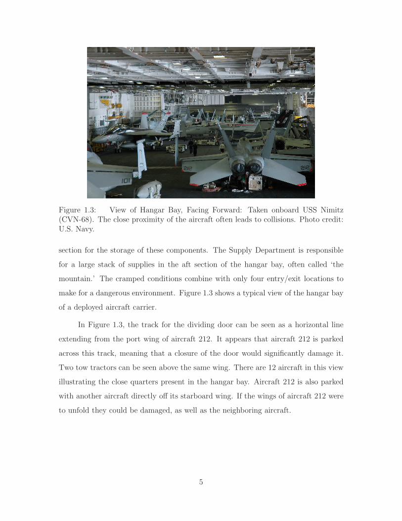
Figure 1.3: View of Hangar Bay, Facing Forward: Taken onboard USS Nimitz(CVN-68). The close proximity of the aircraft often leads to collisions. Photo credit:U.S. Navy.

section for the storage of these components. The Supply Department is responsible

for a large stack of supplies in the aft section of the hangar bay, often called ‘the

mountain.’ The cramped conditions combine with only four entry/exit locations to

make for a dangerous environment. Figure 1.3 shows a typical view of the hangar bay

of a deployed aircraft carrier.

In Figure 1.3, the track for the dividing door can be seen as a horizontal line

extending from the port wing of aircraft 212. It appears that aircraft 212 is parked

across this track, meaning that a closure of the door would significantly damage it.

Two tow tractors can be seen above the same wing. There are 12 aircraft in this view

illustrating the close quarters present in the hangar bay. Aircraft 212 is also parked

with another aircraft directly off its starboard wing. If the wings of aircraft 212 were

to unfold they could be damaged, as well as the neighboring aircraft.

5

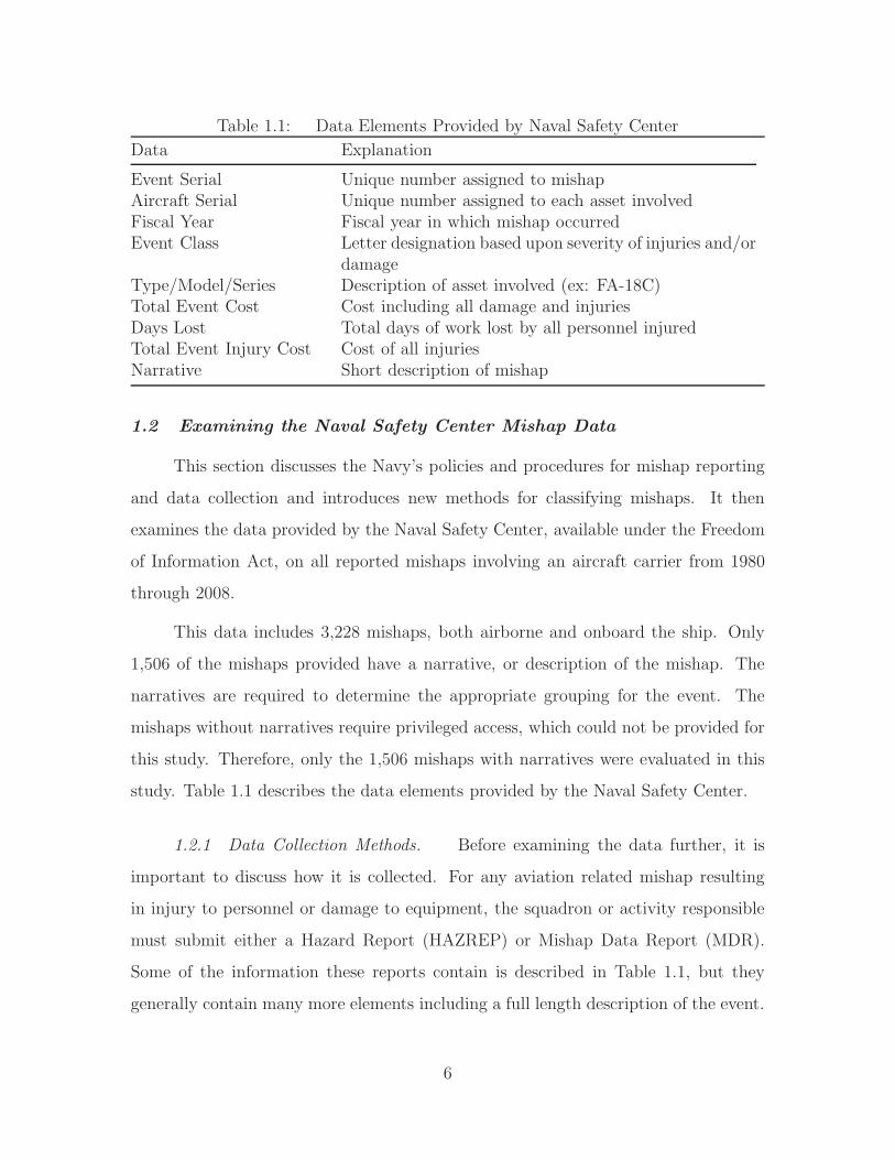
Table 1.1: Data Elements Provided by Naval Safety Center

Data Explanation

Event Serial Unique number assigned to mishapAircraft Serial Unique number assigned to each asset involvedFiscal Year Fiscal year in which mishap occurredEvent Class Letter designation based upon severity of injuries and/or

damageType/Model/Series Description of asset involved (ex: FA-18C)Total Event Cost Cost including all damage and injuriesDays Lost Total days of work lost by all personnel injuredTotal Event Injury Cost Cost of all injuriesNarrative Short description of mishap

1.2 Examining the Naval Safety Center Mishap Data

This section discusses the Navy’s policies and procedures for mishap reporting

and data collection and introduces new methods for classifying mishaps. It then

examines the data provided by the Naval Safety Center, available under the Freedom

of Information Act, on all reported mishaps involving an aircraft carrier from 1980

through 2008.

This data includes 3,228 mishaps, both airborne and onboard the ship. Only

1,506 of the mishaps provided have a narrative, or description of the mishap. The

narratives are required to determine the appropriate grouping for the event. The

mishaps without narratives require privileged access, which could not be provided for

this study. Therefore, only the 1,506 mishaps with narratives were evaluated in this

study. Table 1.1 describes the data elements provided by the Naval Safety Center.

1.2.1 Data Collection Methods. Before examining the data further, it is

important to discuss how it is collected. For any aviation related mishap resulting

in injury to personnel or damage to equipment, the squadron or activity responsible

must submit either a Hazard Report (HAZREP) or Mishap Data Report (MDR).

Some of the information these reports contain is described in Table 1.1, but they

generally contain many more elements including a full length description of the event.

6

These reports are all collected by the Naval Safety Center and stored in a computer

database, AVIATION DATABASE NSIRS.

The purpose of the HAZREP or MDR is to record objective data for analysis

by the Naval Safety Center, but there are numerous reasons why the data contained

in the report may not reflect the totality of reality. Due to the natural desire to

downplay the significance of a mishap and the amount of damage as well as the

inherent difficulty in capturing the true total cost of a mishap, the estimated cost is

typically much lower than one would expect.

The Naval Aviation Safety Program [9] classifies mishaps based upon the number

of workdays lost due to injury or the financial severity of damage to equipment.

Mishaps are also categorized as Flight, Flight-Related, or Aviation Ground Mishaps,

but for the purposes of this research these distinctions are not sufficient. According to

the instructions for this program, a mishap is categorized as Flight or Flight-Related

if the intent for flight existed, not simply if it occurs in the air. A collision between

a sailor or parked aircraft and an aircraft launching from a catapult is reported as

a Flight mishap, but it is still of interest to this research because it is potentially

preventable. On the other hand, a mishap caused by system failure on the aircraft

during launch, also reported as a Flight mishap, is outside the scope of this research.

The severity of the mishap is classified by assigning a letter designator, based

upon cost, as outlined in Table 1.2 [9]. The process of determining the cost of a

mishap is detailed in Section 314 of the Naval Aviation Safety Program [9]. The

reporting activity is directed to “Compute the cost of damage to DoD property using

the best known cost of repair or replacement. Base these cost estimates on the price of

materials and man-hours necessary to repair the damage.” This does little to account

for the cost of lost sorties or lost productivity due to mishap investigation. It is

unclear how to estimate the cost of an extreme case like a sailor being lost overboard.

In the 2008 PBS Documentary Carrier, there was a sailor lost overboard and the

Carrier Strike Group spent three days searching with multiple surface ships as well

7

Table 1.2: Classification Criteria for Aviation Mishaps

Class Damage Requirements Injury Requirements

A > $1, 000, 000 or Aircraft Destroyed Fatal Injury and/or PermanentTotal Disability

B > $200, 000 Permanent Partial Disabilityand/or Three or More PersonnelHospitalized

C > $20, 000 Five Lost Workdays

HAZREP < $20, 000 Beyond First Aid But Less ThanFive Lost Workdays

as U.S. and allied aircraft. The cost of the search effort and loss of life must have

been staggering, considering the cost of operating a CVN is typically thought of as

over $1M per day. It is unclear how the full cost of such an event would be accurately

determined. One must not only account for the fuel consumed by the searching surface

vessels and aircraft but also the cost of tasking those assets with duties other than

the mission of the Strike Group.

It is a common perception in the fleet that there will be negative repercussions

when reporting a mishap, so efforts are often made to minimize the reported value of

damage that occurred. This is usually characterized by extra effort on the part of the

maintainers to repair a component instead of ordering a costly replacement. The dollar

amounts reported for these mishaps may not always represent the actual cost to the

Navy. Even listing the pre-determined cost of a replacement part doesn’t necessarily

capture the full logistics costs associated with its procurement and shipment. These

statements are not intended as a criticism of the Naval Aviation Safety Program but

to make the reader aware that the costs presented in Section 1.2.4 do not completely

capture the total cost.

Even more important than the cost associated with a mishap is the impact it

has on the CVW’s mission. The collision of two aircraft on the flight deck can lead

8

to the loss of scheduled sorties, delays in the scheduled maintenance of other aircraft,

and increased strain on the logistics train. The effect of one mishap is typically felt

for days or weeks as schedules are adjusted with the result being a reduction in the

ability to provide striking power from the sea.

The goal of this research is to evaluate technological improvements which could

be implemented to prevent injury, save lives, and reduce expenses. However, the

incalculable or unrecorded factors in the total cost of a mishap make it difficult to

estimate the true cost benefit of a system designed to prevent mishaps.

1.2.2 Classifying Mishaps. Because the focus of this research is to evaluate

methods to reduce or prevent mishaps, it is necessary to group mishaps into cate-

gories based upon causes, not costs, so that the causes can be targeted for mitigation.

The next step is to evaluate the causes of the mishaps in each category and research

technological improvements that could be leveraged in an attempt to reduce their oc-

currence. A set of categories was created which describes all of the flight deck related

mishaps which could potentially be prevented by applying modern RTLS technolo-

gies. If a narrative described a mishap which the author thought was potentially

preventable, it was marked an Interest Mishap.

In the first step of this research, the narratives of 1,506 mishaps were reviewed

to determine these new classifications. After reading through all available mishap

narratives, the mishaps were either classified into the primary and secondary cate-

gories described below or excluded from further evaluation. These mishap categories

are not exclusive, as some mishaps may fall into multiple categories (primarily when

there is both injury and equipment damage). There were 261 mishaps that fell into

one or more of these categories, which is 8.1% of the total and 14.3% of those with

narratives. It is reasonable to assume that a similar percentage of those mishaps

without narratives would also fall into these categories, since no significant changes

have been made over the period of the recorded data which would have decreased the

rate of occurrence of such mishaps. The primary categories are listed in descending

9

order of total cost of all mishaps falling into that category as reported in the data

provided by Naval Safety Center. The occurrence and mean cost 1 of these categories

is presented in Table 1.3.

Primary Interest Mishap Categories:

1. Spotting: Aircraft is stationary when another object in its normal operation

impacts it or aircraft begins uncontrolled movement due to ship’s motion. (Note:

If an aircraft is towed into another aircraft, it is considered a towing mishap

regardless of the position of the stationary aircraft.)

2. Towing: While under tow, aircraft or tow tractor collides with (non-human)

object. This classification also covers aircraft being pushed into a parking posi-

tion.

3. Taxiing: With pilot in command, aircraft collides with (non-human) object.

4. Exhaust: Aircraft is damaged or sailor is injured by engine exhaust.

5. Contact: A sailor is injured or killed by contact with a moving aircraft (excludes

engine/exhaust contact).

6. Engine: Aircraft is damaged or sailor is injured by contact with turning engine

(usually propeller).

7. Wingfold: The spreading (or folding) of an aircraft’s wings impacts another

object (usually another aircraft).

8. Non-aviation: Aircraft damaged during non-aviation related event, such as an

underway replenishment.

Secondary Categories:

1. Miscellaneous: Any flight deck or hangar bay mishap that does not fall into the

above categories but may still be potentially preventable.

1Cost data used in this research is unchanged from the data provided. As an example, adjustmentsfor inflation are not made.

10

Table 1.3: Occurrence and Average Cost of Mishap Categories: Occurrence givenas percent of total mishaps with narratives (excluding HAZREPS).

Category Occurrence (%) Mean Reported Cost ($)

Spotting 5.19 1,251,800Towing 10.71 335,800Taxiing 8.93 319,100Exhaust 5.03 181,000Contact 4.06 83,800Engine 1.46 60,600Wingfold 0.32 10,900Non-aviation 0.16 1,200

Miscellaneous 2.44 39,800Unknown 1.79 906,100

2. Unknown: Some mishap that could potentially be prevented occurred on the

flight deck or hangar bay but the exact circumstances cannot be determined

from the available information.

Mishaps that have narratives and were identified as belonging to one of these

categories are termed Interest Mishaps for the purposes of this research. To further

illustrate the method by which mishaps were classified based upon their narrative,

an example for each of the primary categories is provided in Table 1.4. The Interest

Mishaps will be examined further to evaluate methods of mishap detection or preven-

tion. The complete list of Interest Mishaps is provided in Appendix A on page 135.

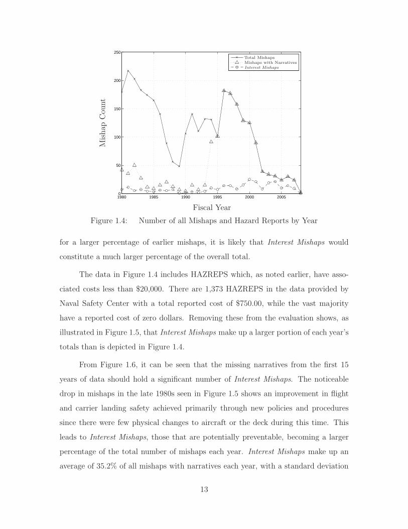
1.2.3 Preliminary Analysis. Figure 1.4 illustrates the trends in mishap

occurrence during the period of time covered by the available data. Total mishaps in-

clude every mishap within the available data2, including airborne mishaps and Hazard

Reports. It is interesting to observe that in more recent years the Interest Mishaps

make up a larger percentage of the total. The primary reason for this is that the more

recent data has a larger percentage with narratives. If narrative data were available

2Few mishaps are listed for fiscal year 2008 as the data was provided early in the fall of 2007.They are included in this analysis for the sake of thoroughness.

11

Table 1.4: Examples of Mishap Narratives and their Classifications: Narratives arepresented exactly as recorded by Naval Safety Center.

Event Serial Fiscal Year Narrative Classification

22273 1986 PARKED ACFT SUSTAINED DAM-AGE WHEN BARRICADE STAN-CHION STRCK HORIZ STAB

Spotting

40688 1994 ACFT UNDER TOW IN HANGARDECK BAY COLLIDED WITHPARKED ACFT.

Towing

47673 1998 ACFT RADOME IMPACTED BYAILERON OF SECOND ACFTWHICH WAS TAXIING ON DK

Taxiing

53357 2001 FLIGHT SURGEON BLOWN OVER-BOARD DURING CQ OPERA-TIONS.

Exhaust

35370 1992 BLUE SHIRT RUN OVER BY ACFTMAIN MOUNT.

Contact

47642 1998 PLANE CAPTAIN STRUCK BYTURNING PROPELLER.

Engine

50548 2000 UNCOMMANDED WING SPREADCAUSED WINGS TO STRIKE ACFTIN CLOSE PROXIMITY

Wingfold

69377 2006 ACFT PARKED ON FLT DECKSTRUCK BY FORK LIFT TRAC-TOR DUR REPLENISHMENT.

Non-aviation

12

1980 1985 1990 1995 2000 20050

50

100

150

200

250

Fiscal Year

Mishap

Cou

nt

Total Mishaps

Mishaps with NarrativesInterest Mishaps

Figure 1.4: Number of all Mishaps and Hazard Reports by Year

for a larger percentage of earlier mishaps, it is likely that Interest Mishaps would

constitute a much larger percentage of the overall total.

The data in Figure 1.4 includes HAZREPS which, as noted earlier, have asso-

ciated costs less than $20,000. There are 1,373 HAZREPS in the data provided by

Naval Safety Center with a total reported cost of $750.00, while the vast majority

have a reported cost of zero dollars. Removing these from the evaluation shows, as

illustrated in Figure 1.5, that Interest Mishaps make up a larger portion of each year’s

totals than is depicted in Figure 1.4.

From Figure 1.6, it can be seen that the missing narratives from the first 15

years of data should hold a significant number of Interest Mishaps. The noticeable

drop in mishaps in the late 1980s seen in Figure 1.5 shows an improvement in flight

and carrier landing safety achieved primarily through new policies and procedures

since there were few physical changes to aircraft or the deck during this time. This

leads to Interest Mishaps, those that are potentially preventable, becoming a larger

percentage of the total number of mishaps each year. Interest Mishaps make up an

average of 35.2% of all mishaps with narratives each year, with a standard deviation

13

1980 1985 1990 1995 2000 20050

50

100

150

200

250

Fiscal Year

Mishap

Cou

nt

Total Mishaps

Mishaps with NarrativesInterest Mishaps

Figure 1.5: Number of all Mishaps by Year (Excludes Hazard Reports)

1980 1985 1990 1995 2000 20050

10

20

30

40

50

60

70

80

90

100

Fiscal Year

Inte

rest

Mis

hap

Per

centa

ge

Percentage of All Mishaps

Percentage of Mishaps with Narratives

Figure 1.6: Occurrence of Interest Mishaps as Percentage of Total Mishaps

14

1980 1985 1990 1995 2000 20050

50

100

150

Fiscal Year

Cos

t(M

illion

sof

Dol

lars

)

Total Mishap Cost

Interest Mishap Cost

Figure 1.7: Cost of Mishaps with Narratives

of 15.93%. Since improved policies and procedures have been unable to significantly

reduce the number of Interest Mishaps over the period of recorded data, improvements

to flight deck safety must be achieved by other means.

1.2.4 Cost of Mishaps. With an understanding of the limitations on the

collection of mishap cost data as described in Section 1.2.1, the cost of mishaps over

the time period available can be evaluated as illustrated in Figure 1.7. Due to the

great difference between Total and Interest Mishap costs, the Interest Mishap costs

are reproduced in Figure 1.8.

A single flight mishap resulting in the loss of an aircraft (or multiple aircraft),

can incur a cost higher than all of the Interest Mishaps over an entire year. With the

aircraft purchase costs in Table 1.5, it is easy to see why. But, the total cost of Interest

Mishaps since 1980 is $92,486,469, 5.55% of the cost of all recorded mishaps in this

data (including those lacking narratives). This should provide significant motivation

to explore means of reducing the occurrence of Interest Mishaps.

15

1980 1985 1990 1995 2000 20050

5

10

15

20

25

30

Fiscal Year

Cos

t(M

illion

sof

Dol

lars

)

Figure 1.8: Cost of Interest Mishaps

Table 1.5: Aircraft Purchase Costs [23]

Aircraft Cost (Millions of $)

FA-18(A-D) 25FA-18(E-F) 43.6EA-6B 55.7E-2C 70

16

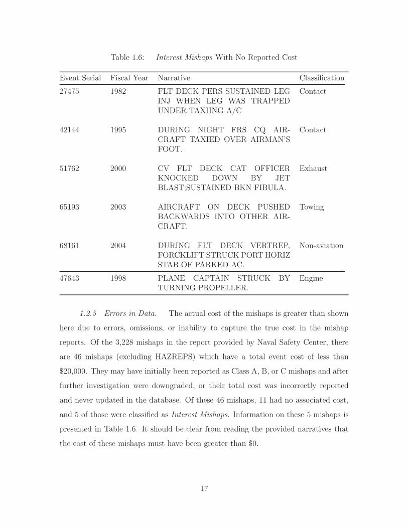
Table 1.6: Interest Mishaps With No Reported Cost

Event Serial Fiscal Year Narrative Classification

27475 1982 FLT DECK PERS SUSTAINED LEGINJ WHEN LEG WAS TRAPPEDUNDER TAXIING A/C

Contact

42144 1995 DURING NIGHT FRS CQ AIR-CRAFT TAXIED OVER AIRMAN’SFOOT.

Contact

51762 2000 CV FLT DECK CAT OFFICERKNOCKED DOWN BY JETBLAST;SUSTAINED BKN FIBULA.

Exhaust

65193 2003 AIRCRAFT ON DECK PUSHEDBACKWARDS INTO OTHER AIR-CRAFT.

Towing

68161 2004 DURING FLT DECK VERTREP,FORCKLIFT STRUCK PORT HORIZSTAB OF PARKED AC.

Non-aviation

47643 1998 PLANE CAPTAIN STRUCK BYTURNING PROPELLER.

Engine

1.2.5 Errors in Data. The actual cost of the mishaps is greater than shown

here due to errors, omissions, or inability to capture the true cost in the mishap

reports. Of the 3,228 mishaps in the report provided by Naval Safety Center, there

are 46 mishaps (excluding HAZREPS) which have a total event cost of less than

$20,000. They may have initially been reported as Class A, B, or C mishaps and after

further investigation were downgraded, or their total cost was incorrectly reported

and never updated in the database. Of these 46 mishaps, 11 had no associated cost,

and 5 of those were classified as Interest Mishaps. Information on these 5 mishaps is

presented in Table 1.6. It should be clear from reading the provided narratives that

the cost of these mishaps must have been greater than $0.

17

Table 1.7: Mandated Injury and Fatality Costs [8]

Personnel Partial Disability ($) Total Disability ($) Fatality ($)

Flying Officer 210,000 1,300,000 1,100,000Other Officers 145,000 845,000 395,000Enlisted 115,000 500,000 125,000

Also shown in Table 1.6 is Event 47643 which was listed as a Hazard Report.

When a person is struck by a turning propeller there is little chance of survival, much

less avoiding significant injury. In fact, this is the only mishap of this type in the data

without an associated fatality or major injury. Without further information, such as

a complete description of the scenario, a detailed analysis of this mishap cannot be

performed. It is presented to illustrate why the true cost of mishaps cannot be easily

determined. One can only hope that since it was reported as a Hazard Report the

sailor survived. There are other mishaps in the data which, based upon the available

data, appear to have discrepancies, but they will be left out of further evaluation.

1.2.6 The Human Cost. The injury-related mishaps in Table 1.6 are sig-

nificant and should be compared to the mandated cost values for similar injuries in

Table 1.7. Interestingly, the mandated costs presented here were last updated in 1988

“so that analysts can make generalized comparisons against historical data” [8].

From the 261 Interest Mishaps, there are 13 fatalities and 34 major injuries. The

major injuries counted here involved sailors being run over by an aircraft, ingested

into a turning engine, or being blown overboard. These numbers were generated from

reading the brief narratives which do not always expressly state the severity of the

injury. A fatality was only recorded if the narrative expressly said the sailor was

killed. Figures 1.9 and 1.10 show the number and recorded costs of fatalities and

major injuries.

Interestingly, the mean cost of both the fatalities and major injuries is below

what would be expected from the mandated costs from Table 1.7 [8]. The mean

18

1980 1985 1990 1995 2000 2005

1

2

3

4

Fiscal Year

Cou

nt

FatalitiesMajor Injuries

Figure 1.9: Number of Fatalities/Major Injuries from Interest Mishaps

1980 1985 1990 1995 2000 20050

1

2

3

4

5

6

Fiscal Year

Cos

t(H

undre

ds

ofT

hou

sands

ofD

olla

rs)

FatalitiesMajor Injuries

Figure 1.10: Cost of Fatalities/Major Injuries from Interest Mishaps

19

fatality cost is $51,462, less than half the mandated amount. This is due to the fact

that through the 1980s the cost associated with the death of an enlisted servicemember

was only $37,000. The mean major injury cost is $82,611. It is not possible to

determine the severity of every injury based upon the available data, but this is still

less than the mandated cost of a partial disability for an enlisted sailor. There are

seven mishaps with associated major injuries that have a cost of zero for injuries. The

narrative for the first of these is “FLT DECK PERS SUSTAINED LEG INJ WHEN

LEG WAS TRAPPED UNDER TAXIING A/C”, which certainly had unreported

associated medical costs.

Beyond the direct medical, life insurance, or disability costs the government

must pay for a mishap involving a fatality or major injury there are other losses that

cannot be calculated with any certainty. A killed or injured sailor affects the perfor-

mance, morale, and retention of those they serve with. Leadership and experience

are lost with a senior member, and their potential with a junior. The effects of these

factors may be difficult or impossible to calculate, but it should be clear that they

are not taken into account when determining the cost of a mishap.

1.2.7 Conclusions From Data Analysis. With the improvements in flight

safety over the last decade, mishaps occurring on the flight deck of an aircraft carrier

are taking an increasing share of each year’s total mishap cost. The annual cost of

Interest Mishaps is consistently in the $2-4 million range, as seen in Figure 1.8, except

for three years where an aircraft was destroyed and the cost was much higher. With

an average of 0.448 sailors killed every year by an Interest Mishap, it is important to

make every effort to prevent them.

By closely examining the data reported to the Naval Safety Center, and an

analysis of its limitations, it has been shown that potentially preventable mishaps,

and their cost, make up a significant percentage of the total each year. This mishap

cost analysis was performed to show that there is still a significant cost every year

to the U.S. Navy for mishaps which have been identified as potentially preventable.

20

This cost analysis is presented as a baseline for the cost benefit of a system that could

predict and potentially prevent mishaps.

1.3 Persistent Monitoring

To prevent mishaps from occurring, it is necessary to provide key personnel with

more accurate and timely data describing the state of all aircraft, equipment, and

personnel on the flight deck and in the hangar bay. To do this, a system must first be

developed to more accurately estimate the aircraft position, orientation, and velocity

than is currently done by the Taxi Director or Handling Officer. Such a system would

be persistent, in that it would continually monitor activities on the flight deck and

hangar bay. This section will explore how modern RTLS technology can be leveraged

to provide a more accurate depiction of state and reduce the occurrence of mishaps

both on the flight deck and in the hangar bay.

1.3.1 Determining Flight Deck State. Since the creation of carrier-based

aviation, the management of the carrier flight deck has been an extremely challenging

task requiring hundreds of personnel each having years of experience. The current

system has changed very little since the 1950s. Personnel on the flight deck use hand

signals to communicate with each other and direct the pilot to make aircraft control

system inputs. The position and orientation of each aircraft are loosely monitored in

Flight Deck Control with objects representing aircraft on a table commonly referred

to as the “Ouija Board” depicted in Figure 1.11. When towing an aircraft personnel

are assigned as Wing and Tail Safeties to ensure the towed aircraft does not impact

another, while the Tow Tractor Driver ensures the route is clear of obstructions.

Currently, the state of each aircraft (position, orientation, and translational/rotational

velocities) is estimated only by a human observer’s judgement.

It is this human-based estimation of state approach which creates a capacity

for mishaps. With a very large quantity of aircraft, SE, and personnel as well as

flight deck surfaces such as jet blast deflectors, elevators, and catapults, the flight

21

Figure 1.11: Flight Deck Represented by a “Ouija Board”: Photo credit: U.S.Navy.

deck naturally lends itself to a computer-based tracking system. Table 1.8 illustrates

many of the elements required for a useful depiction of flight deck state. To reduce

the occurrence of mishaps, it is possible to improve the accuracy of the flight deck

state through the use of modern RTLS. For the purposes of this research, the fidelity

with which such a system can determine the state will be divided into four levels

based upon the capabilities the system would provide, increased expected difficulty,

and cost of implementation. Each successive level would include the capabilities of all

previous levels. Further research beyond this effort would be required to determine

the optimal means of achieving these levels as well as their performance requirements.

1.3.1.1 Level One: Aircraft. The purpose of a Level One observa-

tion system is to reduce or eliminate Spotting and Taxiing mishaps as listed in Sec-

tion 1.2.2. As previously stated, the position, orientation, and translational/rotational

velocities of aircraft on the flight deck are currently determined only by a visual es-

timation. To improve this, a new computer-based system can be developed which

provides measurements of aircraft state in near real-time to Flight Deck Control or

other systems and personnel concerned. Level One would also need to determine the

22

Table 1.8: Elements to Describe Flight Deck State

Element Variable Measurement

Elevator Status [el1, el2, el3, el4] Up/Down/In TransitJBD Status [j1, j2, j3, j4] Up/Down/In TransitCatapult Location [c1, c2, c3, c4]pos Distance of catapult from

launch positionCatapult Status [c1, c2, c3, c4]T Applied TensionBarricade StanchionStatus

[b1, b2] Up/Down/In Transit

Hangar Bay Door Sta-tus

[hbd1, hbd2] Open/Closed/In Transit

Wind Speed vwind Free-stream wind velocityDeck Roll/Pitch [Θ, φ]deck Roll/pitch angle

Aircraft Position [x, y, z,Θ, φ, ψ]ACiLocation and orientationrelative to ship

Aircraft Velocity[

x, y, z, Θ, φ, ψ]

ACi

Translational and rotationalvelocities relative to ship

SE Position [x, y, z, ψ]SEjLocation and yaw relativeto ship

SE Velocity[

x, y, z, ψ]

SEj

Translational and yaw ve-locities relative to ship

Personnel Position [x, y, z]perskLocation relative to ship

Personnel Velocity [x, y, z]perskVelocity relative to ship

23

EL 1EL 2

Figure 1.12: Aircraft Parked Over the Track of Hangar Bay Door One [37]

status of flight deck surfaces, such as the elevation angle of a jet blast deflector or the

location of an elevator. Many different types of RTLS could be leveraged to acquire

this data including radio locating systems and optical scanning.

A computer system provided with the state measurements in the top two sec-

tions of Table 1.8 could be programmed to recognize many potential hazards and

either prevent them or warn of their pending occurrence. For example, given an

aircraft parked in the Hangar Bay across the tracks of Hangar Bay Door One as in

Figure 1.12, the system could prevent the closing of Door One but allow the closing

of Door Two if requested (assuming it is unobstructed). This principle can similarly

be applied to Jet Blast Deflectors, Elevators, and Barricade Stanchions.

Such a system would also be able to track taxiing aircraft and warn of impending

mishaps. Recalling the example of an aircraft turning near the edge of the Flight Deck

in Section 1.1.1, the pilot would have two sources of information to ensure the nose

tire does not go over the edge. If the system uses wingtip location measurements to

calculate aircraft state, it may even be possible to determine the wingfold status of

the aircraft by measuring the distance between wingtips. This could allow a Level

One system to warn of impending Wingfold mishaps.

24

1.3.1.2 Level Two: Support Equipment. A Level Two system adds

the ability to reduce or eliminate Towing mishaps and to further reduce Spotting

mishaps. Many mishaps with collision damage to aircraft involve SE, whether it is a

tow tractor, fire truck, power generator, or forklift. With a system that can determine

the instantaneous position, orientation, and translational/rotational velocities of SE

it would be possible to reduce the occurrence of many Spotting, Towing, and Non-

aviation mishaps. For much of the larger SE, this could be achieved with a system

similar to that used for Level One, but many smaller items of support equipment,

such as weapon carts, may require different treatment.

By adding the state of SE to the system described in Section 1.3.1.1, warnings

could be provided for pending mishaps involving the collision between SE and air-

craft. Reports of unsafe operation of self-propelled SE, such as excessive speed or

unnecessary proximity to aircraft, could be provided to personnel concerned. The

location of smaller SE, such as ordnance carts, could be tracked to warn taxiing pilots

of unsafe areas.

1.3.1.3 Level Three: Personnel. To improve the safety of flight deck

operations for individual sailors, it would be beneficial to determine their instanta-

neous position and velocity relative to hazards caused by aircraft, SE, elevators, jet

blast deflectors, and exhaust plumes. With the rapid, relatively erratic motion of per-

sonnel on deck as well as the requirement for close proximity to aircraft to perform

many critical tasks, the detection of a potential mishap involving personnel could

be the most difficult to determine. Such a system could serve to mitigate Contact

mishaps and reduce the number of flight deck casualties.

If the system described in Section 1.3.1.2 is further enhanced to measure the

point velocity and position of each sailor on the flight deck and hangar bay, many

of the worst mishaps could potentially be prevented. Warnings to the sailor and

leadership could be provided if any sailor gets within a specified perimeter of an

aircraft with engines turning, especially for unauthorized personnel. If a sailor were

25

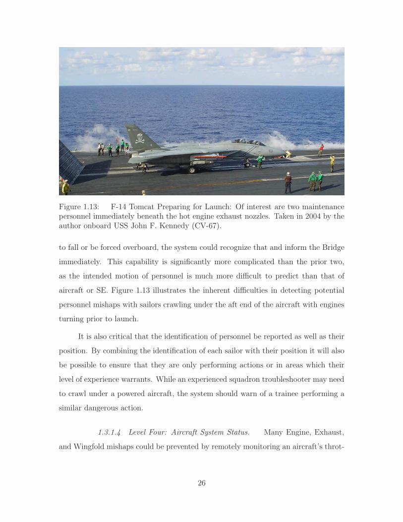
Figure 1.13: F-14 Tomcat Preparing for Launch: Of interest are two maintenancepersonnel immediately beneath the hot engine exhaust nozzles. Taken in 2004 by theauthor onboard USS John F. Kennedy (CV-67).

to fall or be forced overboard, the system could recognize that and inform the Bridge

immediately. This capability is significantly more complicated than the prior two,

as the intended motion of personnel is much more difficult to predict than that of

aircraft or SE. Figure 1.13 illustrates the inherent difficulties in detecting potential

personnel mishaps with sailors crawling under the aft end of the aircraft with engines

turning prior to launch.

It is also critical that the identification of personnel be reported as well as their

position. By combining the identification of each sailor with their position it will also

be possible to ensure that they are only performing actions or in areas which their

level of experience warrants. While an experienced squadron troubleshooter may need

to crawl under a powered aircraft, the system should warn of a trainee performing a

similar dangerous action.

1.3.1.4 Level Four: Aircraft System Status. Many Engine, Exhaust,

and Wingfold mishaps could be prevented by remotely monitoring an aircraft’s throt-

26

Table 1.9: Mishap Cost by Category and Minimum Observation Level

Category Total Reported Cost ($) Mean Annual Cost ($) Mitigating Level

Spotting 36,301,190 1,251,800 1Towing 9,739,576 335,800 2Taxiing 9,225,025 318,100 1Exhaust 5,248,076 181,000 4Contact 2,430,815 83,800 3Engine 1,756,015 60,600 4Wingfold 316,596 10,900 4Non-aviation 35,883 1,200 2

tle or wingfold status. Utilizing a datalink to report necessary aircraft status informa-

tion to Flight Deck Control could provide this capability. There are current systems

to provide this information when an aircraft is powered, but it could prove beneficial

to transmit this information when unpowered.

1.3.2 Benefits. Using the mishap data from Naval Safety Center, this re-

search aims to estimate the cost benefit of implementing such a system. Table 1.9

provides the cost of the different mishap categories and the lowest observation level

which could reduce their occurrence. From the mean annual cost of each category

and the observation level needed to reduce that category, the potential savings of em-

ploying a particular level can be determined as depicted in Figure 1.14. Recalling the

issues with mishap cost data discussed in Section 1.2.4, the dollar amounts described

represent the absolute lowest estimate of potential cost benefits.

Beyond the potential reduction in mishaps there are many additional, significant

benefits to a persistent monitoring system. Such a system could ease the integration

of UAVs into the Carrier Air Wing. The persistent monitoring system would track all

vehicles, manned and unmanned, and could provide a flight deck “map” to unmanned

systems. This could allow UAVs to plan a path to their designated position around

obstacles such as other aircraft and personnel.

27

1 2 3 40

0.5

1

1.5

2

2.5

Observation Level of System Implemented

Million

sof

Dol

lars

Spotting

TowingTaxiing

ExhaustContact

EngineWingfold

Non-aviation

Figure 1.14: Potential Annual Savings of Implementing Observation System

A persistent monitoring system could provide all levels of Naval leadership

with accurate recordings of all flight deck activity. The current reporting system for

mishaps does not document “near mishaps”, or those which were narrowly averted.

Recording and reporting “near mishaps” could become the primary mechanism in

reducing potential mishaps. “Close calls” occur frequently, and if recorded and re-

ported, they could contribute to preventing mishaps through changes in policy, train-

ing, and modifications to the hazard identification algorithms. A complete recording

of flight deck activity would provide the Naval Safety Center with significantly im-

proved documentation on the hazards of flight deck operations, especially for forensic

analysis. It would also provide commanders with detailed records of personnel actions

which can be used to document training and experience, as well as justify manpower

requirements.

1.4 Research Discussion

This section discusses the objectives and assumptions of this research as well as

the methodology used. An overview of this document is presented.

28

1.4.1 Research Objectives. This research intends to be a feasibility study in

which the minimum requirements of a persistent monitoring system for parameters

such as position and orientation measurement precision, translational and rotational

velocity measurement precision, update rate, and computational power are examined

to provide the capability of predicting and warning of potentially hazardous situations.

These requirements are described in more detail in Chapters II and IV.

1.4.2 Assumptions. While this research is concerned with preventing mishaps

aboard aircraft carriers, the tests to gather data were all performed ashore. It is as-

sumed that the differences in aircraft tow procedures afloat and ashore are minimal.

It is also assumed that the tow procedures performed at NAS Oceana, discussed in

Chapter III, are representative of those used across the fleet.

1.4.3 Hypothesis. Mishaps onboard an aircraft carrier present a significant

cost to the Navy and pose a significant risk to personnel. The implementation of a

persistent monitoring system, able to measure the state of the flight deck, has the

potential to recognize and prevent mishaps.

1.4.4 Methodology. Beyond evaluating and establishing the performance

requirements, this research investigates methods by which the different Levels can be

achieved using modern positioning, sensing, and communication technologies, but is

primarily focused on the Global Positioning System (GPS). As an example, an analysis

of the capabilities, limitations, and requirements to achieve a Level One system using

one or more types of modern RTLS such as GPS and pseudo-GPS is performed. These

systems could be combined with video or LIDAR data using sensor fusion to provide

visual confirmation of reported positions. Chapter II describes the capabilities and

limitations of such systems.

To demonstrate the ability of modern RTLS to measure the state of aircraft

and personnel, a series of tests were devised for data collection at both the Air Force

Institute of Technology (AFIT) and Naval Air Station (NAS) Oceana. Described

29

in detail in Chapter III, these tests used highly accurate civilian survey-grade GPS

receivers to measure the position and orientation of an FA-18C Hornet being towed on

the flight line by personnel with flight deck experience. The data collected provides

an accurate depiction of USN aircraft movement procedures as well as the ability to

develop software algorithms which can monitor for and warn of impending hazardous

situations. The analysis of this data, described in Chapter IV, allows a determination

of whether the positioning accuracy and noise levels of the receivers used are sufficient

to predict paths for aircraft and personnel.

GPS was selected as the measurement source for this research as the survey-

grade receivers used are considered to provide “truth data” for the purposes of survey-

ing property. The persistent monitoring system envisioned by this research should be

measurement source agnostic, such that any sufficiently accurate measurement source

can be utilized.

1.4.5 Document Overview. This chapter presented an analysis of safety

records showing the high risk associated with flight deck operations. A persistent

monitoring system was proposed to potentially reduce the occurrence of mishaps.

Chapter II provides a detailed overview of past and present research in fields related

to the development of a persistent monitoring system. The tests conducted and

equipment used are described in detail in Chapter III. The results of these tests are

presented in Chapter IV with conclusions discussed in Chapter V.

30

(a) Flight Deck (b) Hangar Bay

Figure 1.15: CVN Flight Deck and Hangar Bay Without CVW [37]

31

(a) Flight Deck (b) Hangar Bay

Figure 1.16: CVN Flight Deck and Hangar Bay With CVW (notional) [37]

32

II. Literature Review

This chapter presents a study of topics relevant to this research. Proposed

computer-based systems to improve flight deck operations are discussed. Back-

ground information on RTLS such as the Global Positioning System (GPS) and similar

pseudolite systems, as well as methods to determine the position and orientation of an

aircraft based on known GPS receiver location are presented. Algorithms to provide

warnings of hazardous situations are also discussed.

2.1 Flight Deck Systems

Little information is available in open literature on historical and current efforts

to improve flight deck operations with computer-based systems. One possibility for

this is the fact that the U.S. Navy is deeply rooted in tradition. The “Ouija Board”

system of flight deck management described in Section 1.3.1 performs adequately

and is well understood by the personnel involved. Another is that only recently, with

significant advances in RTLS and computers, has a computer-based system to improve

flight deck operations become practicable. This section discusses previous research

into computer-based flight deck management systems, as well as current efforts to

modernize flight deck operations.

2.1.1 Early Research. With a sensing system in place that is able to mea-

sure the flight deck state to one of the four levels discussed in Section 1.3, a means

must be developed to use the state measurement to its greatest potential. Studies of

methods to improve the communication of flight deck state to Flight Deck Control

and other personnel concerned for ‘man-in-the-loop’ control were performed at the

Naval Postgraduate School from 1974-1975 [13,24], the only open literature found on

the subject. These studies did not incorporate RTLS as precise positioning technology

was just being developed.

In 1966, a report was published entitled An Exploratory Study of an Automated

Carrier Aircraft Deck Operation Control System (CADOCS) [43]. This is the first de-

33

Figure 2.1: Proposed Handheld “Flight Deck Data Entry Device”, Circa 1974: byGiardina [13, pg. 54] (from microfiche).

scription of an attempt at using computer systems to improve flight deck operations.

It argued that since many flight deck management operations are repetitive in nature,

they can be performed by a computer. It recognized that the quality of a solution

provided by the computer is dependent upon the quality of the data it is provided.

A variety of stationary and handheld devices used by flight deck personnel were rec-

ommended for data entry. An example of a proposed handheld device is depicted in

Figure 2.1 [13, pgs. 9-10].

The CADOCS concept was further refined in 1967 by the report: Systems Def-

inition Study of Carrier Aircraft Deck Operations Control System [25]. A system

actually capable of generating the aircraft spotting plan for the entire flight deck

based upon maintenance status and flight schedule requirements was proposed. Two

of the unfavorable aspects of CADOCS described by Giardina in 1974 are: inaccu-

racy of position data and performance of existing computers [13, pgs. 10-13]. The

CADOCS system was further refined in two additional reports [42, 44]1.

1The reports on CADOCS ( [25, 42–44]) remain authorized for distribution only to governmentagencies. No information present in this research comes from them directly.

34

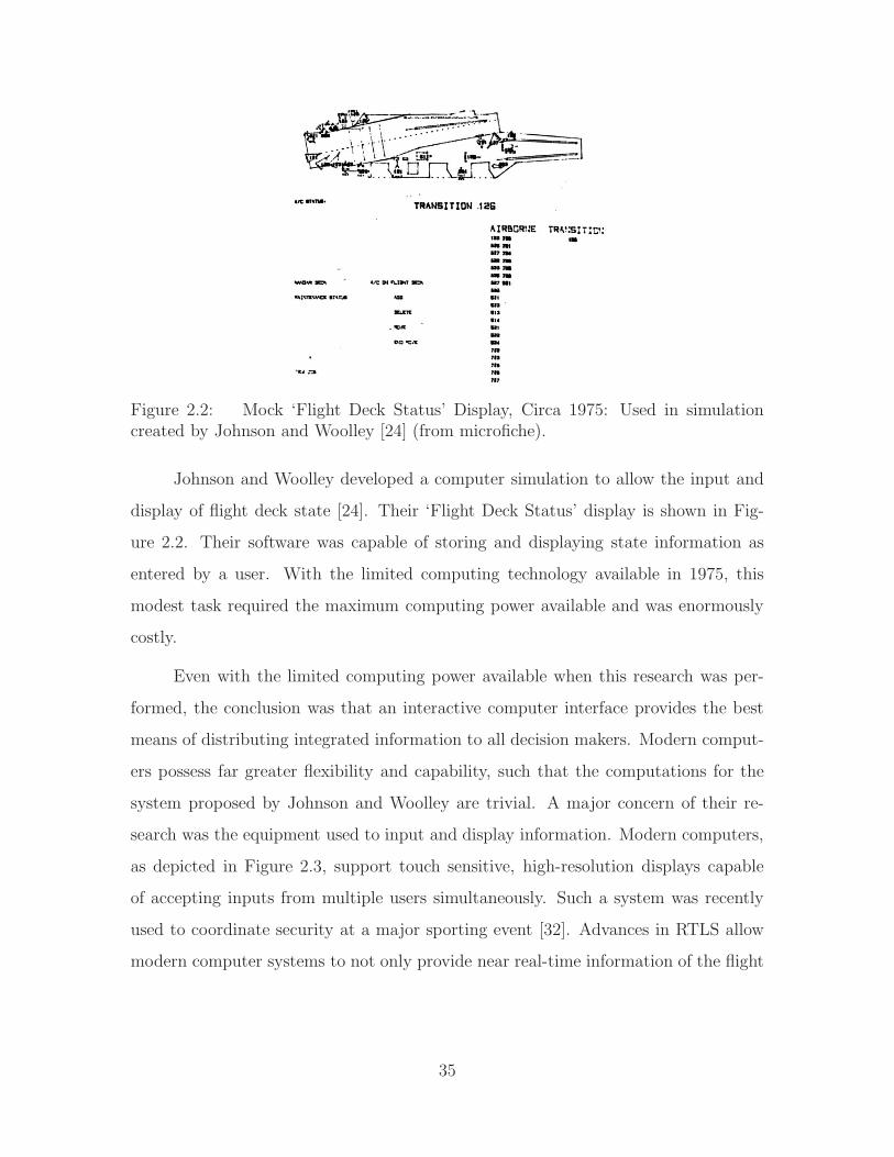
Figure 2.2: Mock ‘Flight Deck Status’ Display, Circa 1975: Used in simulationcreated by Johnson and Woolley [24] (from microfiche).

Johnson and Woolley developed a computer simulation to allow the input and

display of flight deck state [24]. Their ‘Flight Deck Status’ display is shown in Fig-

ure 2.2. Their software was capable of storing and displaying state information as

entered by a user. With the limited computing technology available in 1975, this

modest task required the maximum computing power available and was enormously

costly.

Even with the limited computing power available when this research was per-

formed, the conclusion was that an interactive computer interface provides the best

means of distributing integrated information to all decision makers. Modern comput-

ers possess far greater flexibility and capability, such that the computations for the

system proposed by Johnson and Woolley are trivial. A major concern of their re-

search was the equipment used to input and display information. Modern computers,

as depicted in Figure 2.3, support touch sensitive, high-resolution displays capable

of accepting inputs from multiple users simultaneously. Such a system was recently

used to coordinate security at a major sporting event [32]. Advances in RTLS allow

modern computer systems to not only provide near real-time information of the flight

35

Figure 2.3: Modern Multi-touch, Tabletop Display

Figure 2.4: ADMACS Electronic “Ouija Board” [31]

deck state but also predict and warn personnel of potential hazards based upon the

measured trajectories of aircraft, equipment, and personnel.

2.1.2 Current Developments. A system currently installed on CVNs, Avia-

tion Data Management and Control System (ADMACS), currently provides systems

to track the flight schedule as well as visual records of launch and recovery operations.

The Block 3 upgrade, scheduled for installation on USS Abraham Lincoln (CVN-72)

in fiscal year 2010, will provide an automated, digital “Ouija Board”. Measurements

of aircraft position and orientation will be made by video analysis software. Expected

accuracies of aircraft position measurements are approximately 0.3 m [31].

2.1.3 Carrier-based Unmanned Aerial Vehicles. The problem of UAV in-

corporation on the flight deck is currently being actively pursued by many programs.

36

The Unmanned Combat Aircraft System - Carrier Demonstration (UCAS-D) is a

UAV prototype to demonstrate aircraft carrier launch and recovery capabilities. The

contract was awarded in August, 2007 with a carrier landing attempt planned for

2012 [7, pg. 74]. The method of providing positive control during flight deck opera-

tions is left to the vendor [34, pg. 36].

Venetsky, et al. performed an extensive study on the use of gesture recognition

to enable UAVs to follow the directions of Taxi Directors, as pilots are trained to do.

Each UAV would have a visual sensor mounted on it to watch its assigned director.

There are significant obstacles such as low light, light source blooming, sun glare,

steam, occlusion, and clutter. The results of the study are that such a system is

feasible if visibility of taxi directors is augmented, sensors are placed high on the

aircraft, and Taxi Director practices are more standardized [54].

2.2 The Global Positioning System

This section will provide a brief overview of GPS. It will focus on the basic

system architecture, signals transmitted, methods of determining position, and errors

in the solution. The risks inherent in a system that relies on GPS will be explored as

well as the modernization efforts to mitigate these risks. Comparable foreign systems,

such as the Russian GLONASS and Europe’s Galileo, will not be discussed.

It is assumed that the reader is familiar with the terminology used to describe

the orbit of a satellite. A comprehensive discussion of satellite orbits is provided by

Vallado [53], while a more thorough description of GPS is provided by Misra and

Enge [33].

2.2.1 Architecture. GPS is a passive radio navigation system based upon

measuring the receiver’s position from known radio transmitters, a method called

trilateration, as depicted in Figure 2.5. Provided by the U.S. DoD, GPS allows users

to accurately calculate position, velocity, and time. GPS was originally intended for

U.S. military forces, but as of this writing, civilians are the primary user and it has

37

Signal Broadcast Radius

Receiver Position

Satellite 1

Satellite 2Satellite 3

Satellite 4

ρ1

ρ2ρ3

ρ4

Figure 2.5: Illustration of GPS Passive Radio Navigation: Tracing an arc of equallength from each satellite, the position of the receiver is the only point where everyarc intersects.

become an integral component of the global economy [33, p. 32]. The system is

divided into three segments: space, control, and user.

2.2.1.1 Space Segment. A constellation of 24 satellites (nominal)

transmit pre-defined code sequences, termed Pseudorandom Noise (PRN) code, which

can be acquired and tracked by a GPS receiver. The satellites are in a near-circular

orbit with a radius of 26,560 km. There are six orbital planes, each with at least four

satellites. The orbital planes have an inclination of 55 from the equator. [33, p. 33]

The GPS satellite constellation was designed so that at least four satellites would

be visible from any point on Earth at any time. It is more common that a user sees

38

six to eight satellites at any given time. Built with a design life of 7.5 years, most

GPS satellites have doubled their expected functional lifespan. [33, pp. 33-34]

2.2.1.2 Control Segment. The GPS control segment serves to accu-

rately monitor and predict the orbits of the satellites. Multiple tracking stations are

deployed around the world to measure the satellite orbits. Without the services of the

control segment, the accuracy of a GPS solution would be severely degraded [33, pp.

34-35].

Headquartered at Schriever Air Force Base, the Master Control Station is re-

sponsible for maintaining the currency and accuracy of information transmitted by the

GPS constellation. Updates are normally transmitted to the satellites once daily [33,

pg. 35].

2.2.1.3 User Segment. Anyone with a GPS receiver is part of the user

segment. While originally designed to primarily support military users, the vast ma-

jority of users now are civilians. Aside from automobile and aircraft navigation, GPS

is used in a wide variety of fields such as farming [16], geology [47], and atmospheric

study [18].

The construction of receivers is the domain of corporations and businesses. Ma-

jor manufacturers design and build their own hardware from the specifications pro-

vided by the GPS Interface Control Document (ICD-GPS-200C) [15].

2.2.2 Signals. Each GPS satellite transmits a pre-defined code on one of two

radio frequencies termed L1 (1575.42 MHz) and L2 (1227.60 MHz) [33, p. 37]. The

L2 frequency transmission, termed P(Y) code, is currently encrypted and intended for

military use only. Some civilian receivers, such as those used in this research, are able

to utilize L2 measurements via proprietary methods. The coarse/acquisition (C/A)

code transmitted on L1 is used for the vast majority of GPS position solutions.

39

Table 2.1: Orbital Parameters in GPS Ephemeris Message

Parameter Explanation

M0 Mean anomaly at reference time∆n Mean motion difference from computed valuee Eccentricity

A12 Square root of semi-major axis

Ω0 Longitude of ascending node at weekly epochi0 Inclination angle at reference timeω Argument of perigee

Ω Rate of right ascension

i Rate of inclination anglet0e Reference time ephemeris

The power of the signals transmitted by GPS satellites is extremely low, only

10−16 W of received power on the surface of the earth [33, pg. 42]. Receiving this

signal is roughly equivalent to attempting to see a flashlight shined by an astronaut

in orbit. The only way a receiver can pick the GPS signal out of the background noise

levels is by knowing what signals to look for. Therefore, the Pseudorandom Noise

(PRN) codes transmitted by the satellites are specified in the GPS Interface Control

Document [15].

Each satellite also transmits an ephemeris message containing its orbital pa-

rameters and an almanac message containing the approximate orbital parameters of

other satellites as well as the status of the GPS constellation [33, p. 126]. A section

of the contents of the ephemeris message are contained in Table 2.1 [15, pg. 94].

This information is transmitted in a 50 bps stream, and the ephemeris for a single

satellite can be transmitted in 30 seconds. The complete navigation message contains

both almanac and ephemeris information. Split into 25 frames, each frame containing

1,500 bits, the complete navigation message takes 12.5 minutes to transmit [33, pp.

127-128].

2.2.3 Solutions. There are three primary methods to utilize the signals

transmitted by GPS.

40

2.2.3.1 Code Phase. The primary measurement intended for GPS is

the transit time of a signal from the satellite to a receiver. This is the measurement

used by the vast majority of commercial GPS receivers and requires the use of only

one frequency.

Each satellite transmits a different, pre-defined sequence of 1023 bits, referred

to as chips, and repeats it indefinitely for the C/A-code. A receiver generates the

same sequence of chips and uses it to correlate with the broadcast signal. This allows

the receiver to calculate the transit time of the signal [33, pp. 38-39].

Using the position of each satellite calculated from the ephemeris data [xk, yk, zk],

the transit time of the signal tk, and the speed of light c, it is possible to calculate

the range to the satellite. Due to clock bias in the receiver, each calculated range

is too long or short by an equal amount. Therefore the calculated ranges are called

pseudoranges [33, p. 23]. The pseudorange ρ to the kth satellite can be calculated by

ρk = c · (tk + ∆tcorrections) . (2.1)

The Newton-Raphson method can be used to solve the resulting system of equations

for the receiver’s position [xrcvr, yrcvr, zrcvr] by solving

ρk =

√

(xk − xrcvr)2 + (yk − yrcvr)

2 + (zk − zrcvr)2 + b+ ǫk (2.2)

where b is the receiver clock bias and ǫk represents unknown errors [33, p. 48].

Experiments have shown that the pseudorange solution is capable of three-

dimensional position accuracy on the order of 4 m [33, p. 216]. While very effective,

higher levels of accuracy are required for this research.

2.2.3.2 Doppler Shift. While it is possible to differentiate a time

history of GPS position estimates to calculate a velocity profile, it is often desired to

41

determine an instantaneous velocity. This is possible using the principle of Doppler

shift.

Satellites in the GPS constellation travel in their orbits at approximately 4

km/s. This motion provides a consistent doppler shift in the transmission frequency

when a receiver is stationary. A receiver in motion can measure a difference from this

nominal frequency. The receiver velocity vrcvr can be calculated by

˙ρ = G

vrcvr

b

+ ǫφ (2.3)

where ˙ρ is a vector containing the rate of change of each pseudorange calculated,

b is the rate of change in the receiver clock (m/s), and ǫφ represents errors in the

pseudorange rate calculation. G is a matrix containing estimated line-of-sight unit

vectors from the receiver to each satellite, given by

G =

−11 1

−12 1...

−1k 1

(2.4)

and

1k =[xk − xrcvr, yk − yrcvr, zk − zrcvr]

|xk − xrcvr|. (2.5)

The rate of change of each pseudorange can then be used to calculate local

frame velocities just as pseudoranges are used to calculate local frame coordinates in

Equation (2.2) [33, pgs. 203, 204, 218-219].

2.2.3.3 Carrier Phase. While code phase measurements use the chips

contained in the unique signal of each satellite, carrier phase measurements use the

difference in phase between the receiver generated signal and the signal received from

42

the satellite. Each chip of the C/A code is 293 m along the length of the broadcast

signal, but a single cycle of the L1 frequency is only 19 cm [4, pg. 21]. This allows

for a much more accurate measurement of the signal’s transit time, leading to a more

accurate position solution.

For a carrier phase measurement, the receiver must measure the initial fractional

phase difference between the signals and track all changes to this measurement. This

way the phase of a received signal can be related to the phase at time of transmission.

The phase offset as a function of time φ(t) is computed from

φ(t) = f · τ +N (2.6)

where f if the carrier frequency and τ is the transit time of the signal, and N is the

integer cycle ambiguity [33, pg. 153].

Carrier phase measurements are ambiguous, leading to the integer ambiguity

term N in Equation 2.6. The integer ambiguity represents the number of whole

cycles of the carrier signal, and based upon the calculated transit time τ it could be a

large number of cycles. Resolving this integer ambiguity usually requires a stationary

receiver in a known location which collects accurate data on the motion of available

satellites [4, pg. 6]. The details behind carrier phase ambiguity resolution are beyond

the scope of this document, but are given by Misra and Enge [33]. When using

carrier phase a receiver is able to provide a position solution with centimeter level

accuracy [33, pg. 234].

2.2.4 Errors. This section discusses the major errors in the GPS solution

and methods to mitigate them. These errors must factor significantly into any per-

sistent monitoring system implemented for the flight deck if it used GPS or another

radio navigation system. Errors in the GPS solution generally fall into one of three

groups [33, pg. 155]:

1. Broadcast message errors,

43

2. Signal propagation uncertainty, and

3. Measurement errors.

Broadcast message errors typically are associated with incorrect parameters in

the ephemeris message [33, pg. 156]. The prediction of satellite orbits is very accurate

for the two-body problem, where only the Earth and a satellite are considered. How-

ever, each satellite is affected by the gravity of every celestial body. Corrections for

many of these factors are contained within the broadcast ephemeris message, such as

the effect of lunar and solar gravity which can account for 25 m of orbital perturbation

after only one hour [33, pg. 124-125]. Currently, the broadcast ephemeris can provide

2 m accuracy in pseudorange measurements [33, pg. 127].

Signal propagation uncertainty errors are caused by the Earth’s atmosphere’s

ability to change the velocity of radio signals, and the pseudorange method described

in Section 2.2.3 requires a constant signal velocity. The upper layer of the atmosphere,

from 40-100 km, is known as the ionosphere and contains free electrons which can

slow the speed of a radio wave. The lower region of the atmosphere, or troposphere,

is much denser and contains relatively large amounts of water which can refract a

radio signal. The effects of both the ionosphere and troposphere vary with time and

location on the Earth [33, pg. 157-158].

There are two primary measurement errors which affect a receiver: noise and

multipath. Receiver noise is the reception of unrelated signals in the frequency band

of interest. The receiver can only see the sum of the signal of interest and the noise

received with it. If the noise is strong enough, the receiver could lose lock on the signal,

or if their signal strength is of the same order, the signal could be misinterpreted.

Signals from satellites low on the horizon are received with less power than those

with higher elevation angles and are more prone to noise [33, pg. 175].

Multipath is the greatest error source in GPS, after applying correction factors,

as of this writing. It is caused by the reflection of a GPS signal so that it reaches

a receiver on multiple paths. Receiving the same signal at multiple times, such as

44

receiving the line of sight signal and one reflected from the ground, adds the additional

reflected distance to the pseudorange measurement. In highly reflective environments,

such as the flight deck of an aircraft carrier, the error in pseudorange measurements

can be as great as 5 m while carrier phase measurement errors can be as high as 5

cm [33, pg. 175-177].

2.2.5 Error Mitigation. Each of the error sources listed in Section 2.2.4

can be corrected for or mitigated through a variety of techniques. This section will

provide a background on GPS error mitigation techniques.

The correction of broadcast message errors is the domain of the Control Seg-

ment, and improvements in satellite tracking will provide improved measurements to

all users, without the need for a receiver upgrade. As an example, when six monitoring

stations operated by the National Geospatial-Intelligence Agency (NGA) were added

in 2005 the quality of predicted orbits was improved [33, pg. 126]. Another method to

improve the estimate of satellite locations is to use precise ephemerides, produced by

the NGA and the Naval Surface Warfare Center. These are post-processed satellite

position measurements, which after only three hours for calculation and dissemina-

tion, can provide satellite position errors of less than 5 cm [33, pg 127].

The errors caused by the troposphere and ionosphere can be mitigated, with

varying success, by applying modeled error corrections. The Klobuchar model can

be used to model ionospheric errors using parameters contained in the broadcast

navigation message. This model is able to reduce the pseudorange measurement error

by nearly 50%, but this can be 10 m on a normal day [33, pgs. 168-169]. Tropospheric

errors can also be mitigated by a model or mapping function, yielding a residual error

of 5-10 cm.

If a receiver is capable of acquiring both GPS frequencies, then the ionospheric

error can be effectively eliminated. Each frequency is affected differently by the

ionosphere, so the signal delay can be calculated [33, pg. 166]. This actually allows for

45

Table 2.2: Effect of Differential GPS on Measurement Errors

Source Potential Size (m) Residual Error (m)

Ephemeris 2 0.1Ionosphere 2-10 0.2Troposphere 2.5 0.2

precise, continual tracking of ionospheric activity, as well as improving the position

solution [18].

2.2.6 Differential GPS. Given a GPS receiver in a known position, referred

to as a base station, it is possible to estimate the errors discussed in Section 2.2.4

that are present in the solution [33]. For a near real-time differential GPS correction,

it is necessary to have a datalink between the base station and the mobile receivers

to which the corrections are to be applied. Many commercial survey-grade receivers,

including those used in the tests described in Chapter III are capable of applying

differential corrections in near real-time. It is also possible to apply the corrections

to recorded data in post-processing. This can be done by software such as NovAtel

Waypoint GrafNavTM [40] or GPStk [51].

The use of differential GPS corrections significantly decreases the amount of

error in the position solution, as shown in Table 2.2. The errors estimated by the

base station are only valid for measurements made near the base station, but in

the case of an aircraft carrier flight deck all measurements would be made near the

base station. The use of differential GPS also provides measurements needed for

carrier phase integer ambiguity resolution, as discussed in Section 2.2.3.3. When

they are combined the solution is often referred to as Carrier-Phase Differential GPS

(CDGPS) [4, pg. 6].

2.2.7 Solution Quality. The geometry of the GPS satellites used by a re-

ceiver for its solution has a significant impact on its precision. GPS satellite geometry

refers to the configuration of the visible constellation, such as satellite elevation rel-

46

ative to the horizon, angular separation, and total number of visible satellites. A

“good” satellite geometry would have 6 − 8 satellites all above 15 − 18 elevation,

and with at least 5 − 10 of angular separation between satellites. As discussed in

Section 2.2.4, measurements made using signals from satellites low on the horizon are

more susceptible to tropospheric error. The satellite geometry can be quantified by

the matrix H [33, pg. 207], calculated by

H =(

GTG)

−1(2.7)

where G is given by Equation 2.4. The geometry quality measurement, or Dilution of

Precision2 (DOP) can be calculated from the elements of H by

D =√

H11 +H22 +H33. (2.8)

DOP is useful as a simple, scalar measure of the satellite geometry used in the

solution. A lower DOP implies a better satellite geometry. The GPS Control Segment

provides maps showing nationwide and worldwide maximum DOP. An example is

given in Figure 2.6.

2.2.8 Limitations. There are many limitations to the use of GPS. Due to

the weak signal strength a receiver generally requires a clear, unobstructed view of the

sky. This generally prevents GPS from being used for indoor positioning. Another

limitation is the requirement for continual updating of GPS ephemeris data by the

Control Segment. The Control Segment has continuously updated ephemeris data for

over twenty years, but it is presented as a limitation because it is a single point of

failure.

A limitation which is the subject of much discussion by military users is the

jamming of GPS signals, especially intentional jamming by enemy forces. Simply

2For this research, the term DOP is synonymous with Position DOP, or PDOP.

47

Figure 2.6: World DOP Assessment [52]

48

broadcasting a high power signal on the L1 frequency can prevent the acquisiton of

GPS signals by all users in range.

2.2.9 Modernization. Efforts to modernize GPS, first announced in 1998,

have the potential to significantly improve its performance for all users, military

and civilian. For civilian users, an unencrypted signal will be broadcast on the L2

frequency, called L2C. The first satellite capable of broadcasting L2C was launched in

2005. This will allow for civilian receivers to eliminate ionospheric error in a manner

similar to military receivers. In addition, a new signal, L5 will be broadcast on 1176.45

MHz. It it a wider bandwidth signal, allowing for better carrier phase positioning,

and will be broadcast with more power than L1 or L2 signals [33, pgs. 73-77].

These improvements, when completed, will enable the mass production of re-

ceivers that have the capability of advanced military or civilian surveying systems.

Given the worldwide demand for precise positioning, it is likely that receivers with

dramatically increased position accuracy will be available in extremely small form

factors.

2.3 Pseudolite Positioning

As discussed in Section 2.2, precise positioning with GPS (e ≤ 1 cm) requires a

carrier-phase solution and a differential correction. Pseudolites provide a method of

achieving precise positioning that does not depend exclusively on the GPS constella-

tion. This section will provide a brief description of the theory behind pseudolites,

their benefits, and limitations. A more thorough overview of pseudolites is provided

by Cobb [4].

2.3.1 Theory. Pseudolite is a term used to describe a radio broadcasting

system, not in orbit, which transmits signals capable of being used by a RTLS (gen-

erally GPS) receiver. Pseudolites operate on the same principle as GPS: trilateration.

When GPS was being developed pseudolites were used in place of unlaunched satel-

49

lites [4, pg. 13]. Given sufficient pseudolites in known locations a code or carrier phase

solution can be computed using the same algorithms described in Sections 2.2.3.1 and

2.2.3.3, and differential corrections can be provided. A pseudolite can generate its

own PRN code, or simply rebroadcast a replica of a received signal [4, pg. 28]. Using

a pseudolite system with rebroadcasting, navigation is possible with three pseudolites

and only one GPS satellite [4, pg. 34].

2.3.2 Benefits. The primary advantage of pseudolites is that they don’t need

to be launched into orbit. Satellite launches cost millions of dollars, but a pseudolite

can be made operational for roughly $1,000 [4, pg. 9]. Furthermore, pseudolites are

not governed by orbital dynamics and can be placed in any configuration desirable, as

long as there is sufficient structure to support them. Pseudolites are able to provide

positioning indoors where GPS satellite signals cannot be received, and are even used

in subterranean mining operations [4, pg. 125].

Pseudolites do not have to transmit GPS compatible signals. Position solution

accuracy could be improved by increasing the chipping rate for code phase measure-

ments or the carrier frequency for carrier phase solutions. Increasing the frequency by

a factor of ten would allow for carrier phase accuracy at the sub-millimeter level [4, pg.

130].

2.3.3 Limitations. Recalling from Section 2.2.2 that GPS signals are re-

ceived with extremely low power levels, having a pseudolite nearby can overwhelm a

receiver with broadcast power. Cobb’s Near/Far Problem describes a scenario where

a receiver far away from the pseudolite cannot track its signals, but a receiver near

the pseudolite cannot receive signals broadcast by GPS satellites [4, pg. 50]. Be-

tween these near and far boundaries both GPS satellite and pseudolite signals can

be received. Most consumer GPS receivers, designed for the low power of GPS satel-

lites, do not possess the dynamic range needed to receive GPS and pseudolite signals

simultaneously [4, pg. 53].

50

There are numerous methods to mitigate the Near/Far Problem. Pseudolite

signals can be transmitted outside of the L1 or L2 frequency bands, or simply offset [4,

pg. 58]. The pseudolite transmission frequency can also hop between different regions

of the L1 or L2 bands. The mitigation technique which can virtually eliminate the

constraints of the Near/Far Problem is to use pulsed pseudolite signals [4, pg. 6]. For

this method, the pseudolite is simply designed to transmit a certain percentage of the

time. According to Cobb, most existing receivers would track both GPS satellite and

pseudolite signals given the proper percentage [4, pg. 62].

One other limitation of pseudolites is geometry. While tropospheric errors aren’t

a concern due to the relatively short distances involved, the need for signals from high

above the horizon is still present. Using exclusively ground based pseudolites, altitude

could not be determined, and an altitude would need to be assumed to determine the

two-dimensional position.

Pseudolite receivers are also susceptible to multipath error. In reflective envi-

ronments, such as the flight deck of an aircraft carrier, the effect of multipath error

on the position solution may be increased, depending on the transmission power and

frequency used.

2.4 Blue Force Tracking

The persistent monitoring system proposed by this research shares many fea-

tures of the U.S. Army’s Blue Force Tracking (BFT) system. BFT uses GPS and

satellite communications to relay the positions of U.S. and coalition forces to each

other as well as command headquarters [45]. Similarly, the persistent monitoring sys-

tem proposed here would provide Flight Deck Control with an accurate measurement

of the state of the flight deck. There are significant differences in scale, communication

range, and accuracy required.

The Army planned to field 40,000 tracking systems by 2008 [45]. Each of these

systems communicate via L-band communication satellites to provide near real-time

51

information to commanders anywhere in the world [50]. This presents a significant

use of the military’s available satellite communications capacity. To meet the goals

of BFT, precise GPS measurements are not required; the accuracy provided by pseu-

dorange measurements is sufficient. Additionally, since not all combat operations

take place outdoors, BFT units utilize an inertial measurement system when GPS is

unavailable.

One significant issue with BFT has been the lack of interoperability [45]. Sys-

tems used by ground vehicles and rotary-wing aircraft often can’t communicate [50].

An entirely different project, the Movement Tracking System (MTS), locates sup-

ply and maintenance vehicles and was not compatible with most BFT systems. The

United States Marine Corp (USMC) used the Mobile Data Automated Communica-

tions system and had to install BFT systems during Operation Iraqi Freedom so they

would be visible to coalition command centers [45].

The principle of BFT is “that if you could display your location, your buddies’

locations and, with intelligence, enemy locations, commanders and soldiers could

achieve a level of communication and information integration that would let you fo-

cus on your real jobs - commanding and warfighting.” [49]. Users of the system, from

the Army, USMC, and United Kingdom claim it saved lives and simplified coordina-

tion [45].

2.5 Determining Position and Orientation

The position and orientation of an aircraft relative to a fixed location on the

deck can be determined using two GPS receivers mounted on the wingtips. Since the

aircraft is not flying, its roll and pitch can be ignored and the problem can be treated

as two-dimensional. In Figure 2.7, the position of each receiver on the wingtips is

denoted by (x1, y1) and (x2, y2). The length of the wingspan b applies a constraint to

the receiver positions given by

52

x

y

O

r1

r2

rc

bb2

ψ

(x1, y1)

(x2, y2)

Figure 2.7: Determining Position and Orientation: Applicable to an aircraft withwingtip mounted receivers.

53

b2 = (x2 − x1)2 + (y2 − y1)

2. (2.9)

Using vector addition, the following relationships can be derived from Figure 2.7

(x1, y1) = (xa, ya) −b

2(cosψ, sinψ) (2.10)

and

(x2, y2) = (xa, ya) +b

2(cosψ, sinψ) (2.11)

where (xa, ya) is the location of the aircraft’s center and ψ is the aircraft’s heading

measured from the x-axis. Subtracting Equation 2.10 from Equation 2.11 yields

(x2 − x1, y2 − y1) = (b cosψ, b sinψ) . (2.12)

Rearranging Equation 2.12 provides

b sinψ

b cosψn

= tanψ =y2 − y1

x2 − x1(2.13)

and

ψ = arctan

(

y2 − y1

x2 − x1

)

. (2.14)

With ψ calculated by Equation 2.14 the center position (xa, ya) can be calculated

by rearranging Equation 2.10 which yields

(xa, ya) = (x1, y1) +b

2(cosψ, sinψ) . (2.15)

54

2.6 Determining Distance - The Nearest Neighbor Problem

Given coordinate sets (x1, y1, z1) and (x2, y2, z2) describing the location of two

points in three-dimensional Euclidean space relative to some reference frame, the

distance between the points can be calculated by the Euclidean- or two-norm from

r =

√

(x2 − x1)2 + (y2 − y1)

2 + (z2 − z1)2. (2.16)

When determining the distance between two three-dimensional objects, one must first

determine which point(s) describing the object should be used. For objects whose size

is much smaller than the distance between them, it may be desirable to use the center

of mass. For the case where personnel are moving in close proximity to an aircraft,

using the aircraft’s center of mass does not provide a useful solution. A more useful

calculation of distance between personnel and the aircraft requires the determination

of the closest point on the aircraft to the personnel. This is a common problem in

algorithms known as the Nearest Neighbor or Post Office Problem [1]. Figure 2.8

illustrates the concept of the Nearest Neighbor Problem in two dimensions.

To issue warnings to personnel in hazardous situations, it is necessary to know

when personnel are dangerously close to hazardous regions around an aircraft, such as

exhaust plumes, engine intakes, etc. Determining which point describing the outline

of an aircraft to use for the distance measurement creates a challenging problem. A

simple first approach at a solution, best described as a “brute force” approach, is to

calculate the distance to every point using Equation 2.16 and then use the smallest

resulting value as the distance between the personnel and aircraft. This is usable

for aircraft outlines with relatively few points, but as the resolution of the outline

increases, the computing power required for this solution will grow with it.

2.6.1 Nearest Neighbor Computation Time. According to Arya, et al. [1]

the amount of computation time required for the “brute force” approach is on the

order of O(dn) where d is the dimension of the vector representing each point, n is

55

Personnel

Personnel

rsafe

r1 r2

r3

r4

r5

Figure 2.8: The Nearest Neighbor Problem: How to find which point on the aircraftto use for distance calculation.

56

0 50 100 150 200 250 300 350 400 450 5007

7.5

8

8.5

9

9.5

10

10.5

Vector Dimension d

CP

UT

imeO

(µs)

Mean TimesBest Fit: O(d)

Figure 2.9: Time to Calculate Euclidean Norm

the number of points to be evaluated, and O(d) is the time required to compute the

distance between two points. To determine O(d) for the MATLABr norm function, a

series of 500 norms were computed for vectors of increasing dimension and the time

to calculate measured and stored. This process was repeated 1,000 times, and the

mean calculation time for each size vector was computed. The results are presented in

Figure 2.93. Listing B.1 on page 151 provides the MATLABr source for this operation.

Fitting a polynomial to the collected data in a least-squares sense provides the

equation for O(d) plotted in Figure 2.9. The nonlinear coefficients of O(d) are ex-

tremely small, so the mean computation time required for a single distance calculation

measured in µs can be approximated by a linear function, given by

O(d) ≃ 0.0047 · d+ 7.5063. (2.17)

This research is primarily concerned with planar and spatial positioning, so only

the two- and three-dimensional nearest neighbor solutions are to be evaluated. From

3Calculations performed on 1.6 GHz Intel Core 2 Duo with 2 GB SDRAM

57

Equation 2.17, the mean computation times for the two- and three-dimensional cases

are 7.5157 and 7.5204 µs, respectively. The three-dimensional case represents a 0.06%

increase in computation time. This is a trivial increase, so the use of three-dimensional

models does not incur a significant performance decrease over two-dimensional models.

The number of points used to describe the aircraft can have a significant impact

on the calculation time. For an aircraft model with n points, the time required for the

“brute force” approach is described by O(dn), and while the linear approximation of

Equation 2.17 holds for dn ≤ 500, for two- and three-dimensional models that is only

250 and 166 points, respectively. Given a higher resolution three-dimensional model,

where n = 100, 000, the mean computation time would be significant. Clearly, when

the motion of approximately 100 personnel around 65 aircraft is considered, this may

require extensive computational power.

2.6.2 Nearest Neighbor Algorithms. The Nearest Neighbor problem has

been discussed in computer science literature for decades, with much of the early

work being done by Friedman, et al. in 1975 [12]. Before discussing algorithms in

detail, it is important to describe the terms used and their relation to this research.

Prototypes are the set of points from which the nearest is desired, or in this research

the set of points describing the geometry of an aircraft or hazard. The test point

is the point from which the nearest neighbor distance is to be calculated, or in this

research the personnel on the flight deck.

The work of Friedman, et al. [12] provides an algorithm which projects each

point along one coordinate axis. Each prototype is examined based on its projected

distance, along the sorted coordinate, from the test point. If the distance of a proto-

type from the test point along this axis is greater than the full-dimensional distance

of previously analyzed prototypes, then no more prototypes need be considered.

As an example, consider the two-dimensional case with a test point at the origin

(x, y)tp = (0, 0). The prototypes described by projected points (x, y)p = (−3, 3),

(−1, 0), (0.5, 0.5), (2, 3), and (3, 2) are sorted in order of their x-values. It is possible

58

to start the algorithm with any point, but for this example the second point will be

selected. Computing the distance of the second prototype from the test point using

the Euclidean norm of Equation 2.16 yields a distance of 1. Now any prototypes

for which abs(x) > 1 can be eliminated. This leaves only one other prototype to

consider, (0.5, 0.5). Compute the distance of all remaining prototypes from the test

point and the prototype with the smallest distance value is the nearest neighbor.

Clearly (0.5, 0.5) is the nearest neighbor as its Euclidean distance from the origin is√

12. The efficiency of this algorithm comes from eliminating, in this example, three

of the five prototypes after only one distance calculation.

The result of tests performed by Friedman, et al. show that in a two-dimensional

case only 20% of the CPU time needed for a “brute force” search is required for 100

prototypes and 4.5% for 1000 prototypes. In the three dimensional case the percent-

ages of the “brute force” times required are 30% and 10%, respectively. Clearly, this

provides significant savings as the resolution of aircraft model geometry increases.

Current research on the Nearest Neighbor problem focuses on high-dimension

searching. Friedman, et al. showed in 1977 that computation times of O(logn) are

achievable, but only for lower dimensions. [1]. Since higher dimensions are not relevant

to this research, well established algorithms for lower dimension nearest neighbor

analysis can be used without sacrificing computational efficiency.

2.7 Path Planning

Path planning refers to the process of using a computer to calculate a path

from one state to another while following specified rules. For a persistent monitoring

system to warn of pending hazards, it would need to be able to predict the path

of aircraft taxiing or being towed on the deck. Path planning is usually presented

in literature as a two-dimensional translational motion problem. As an example, a

vehicle lies on a plane, such as a car in a parking lot, and starts at point (0, 0). It

is desired for the vehicle to go to point (100, 100). The obvious solution is a straight

line, but it is not always possible as there may be obstacles or boundaries the straight

59

0 10 20 30 40 50 60 70 80 90 100

0

10

20

30

40

50

60

70

80

90

100

x

y

Start

End

Figure 2.10: Path Planning Example Scenario

line crosses. For this example, there exists a circular obstacle of radius 10 with its

center at point (50, 50). This scenario is depicted by Figure 2.10.

This section will present an overview of path planning algorithms. A simple

example will be provided and its limitations will be discussed. A more robust and

powerful method, developed by Ross, et al. [29] will also be discussed.

2.7.1 Simple Example. Given the scenario depicted by Figure 2.10, it is

possible to plan a simple path which avoids the obstacle and attains the desired state

(x, y)f = (100, 100). The method presented here is described by Fox, et al. [11]. This

example will illustrate many of the basic principles of path planning as well as the

limitations of linear approaches.

The first step is to generate an initial path. This is simply a line from the start

point to the end point, described by y = mx+ b where m is the slope of the line and

b the y intercept. It is clear that in this simple example m = 1 and b = 0.

Next, the initial path must be checked for collisions with any obstacles. A series

of test points are chosen along the initial path. Starting with the test point nearest

60

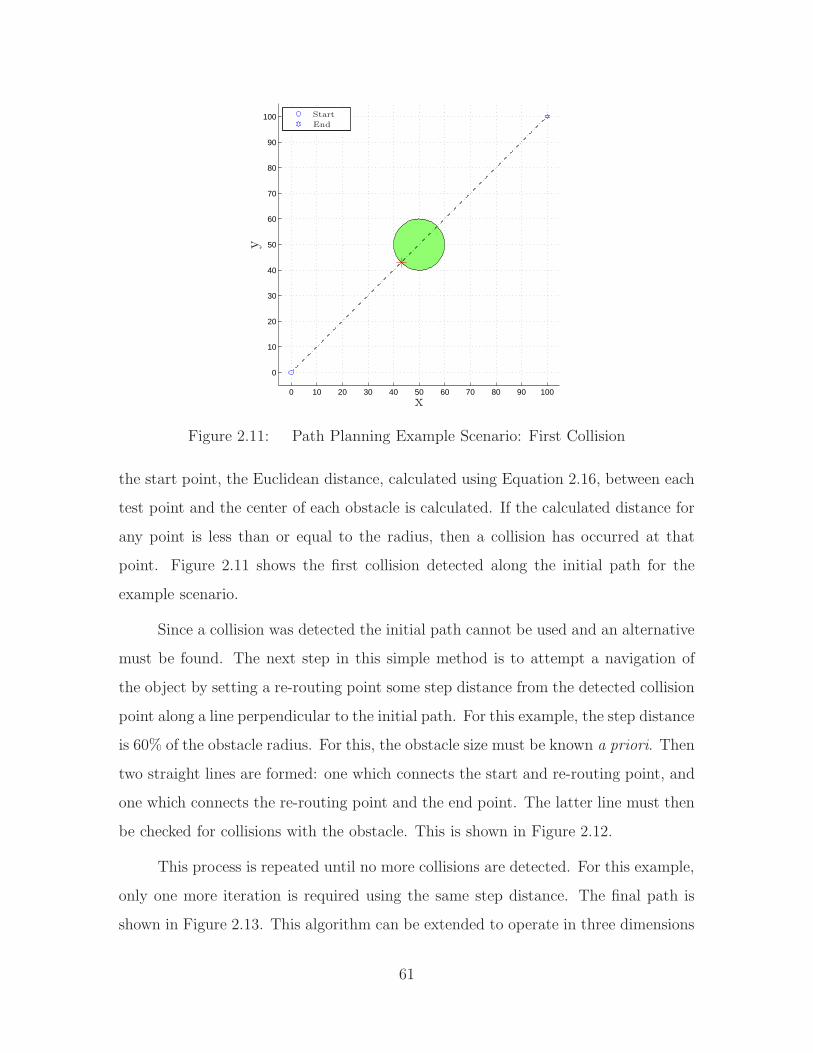
0 10 20 30 40 50 60 70 80 90 100

0

10

20

30

40

50

60

70

80

90

100

x

y

Start

End

Figure 2.11: Path Planning Example Scenario: First Collision

the start point, the Euclidean distance, calculated using Equation 2.16, between each

test point and the center of each obstacle is calculated. If the calculated distance for

any point is less than or equal to the radius, then a collision has occurred at that

point. Figure 2.11 shows the first collision detected along the initial path for the

example scenario.

Since a collision was detected the initial path cannot be used and an alternative

must be found. The next step in this simple method is to attempt a navigation of

the object by setting a re-routing point some step distance from the detected collision

point along a line perpendicular to the initial path. For this example, the step distance

is 60% of the obstacle radius. For this, the obstacle size must be known a priori. Then

two straight lines are formed: one which connects the start and re-routing point, and

one which connects the re-routing point and the end point. The latter line must then

be checked for collisions with the obstacle. This is shown in Figure 2.12.

This process is repeated until no more collisions are detected. For this example,

only one more iteration is required using the same step distance. The final path is

shown in Figure 2.13. This algorithm can be extended to operate in three dimensions

61

0 10 20 30 40 50 60 70 80 90 100

0

10

20

30

40

50

60

70

80

90

100

x

y

Start

End

Figure 2.12: Path Planning Example Scenario: Second Collision

and with obstacles other than circles. It will find a path for a sufficiently simple

arrangement of obstacles.

This simple algorithm has many disadvantages and limitations. It requires com-

plete knowledge of the environment, and the environment must be stationary, and yet

this knowledge is not used to its full extent. It also makes no consideration for vehi-

cle dynamics. The step distance can be arbitrarily large or small, and may have no

basis in the capabilities of the vehicle for which the path is being planned. Addition-

ally, the inability of this simple algorithm to find a path which avoids all obstacles is

insufficient to prove a path does not exist.

2.7.2 Proposed Methods. The focus of much path planning research is in the

area of robotics. Areas of focus include wheeled mobile robots [28] and UAVs [56]. The

algorithm illustrated in Section 2.7.1 is used in the Strategic-Tactical-Execution Soft-

ware Control Architecture (STESCA) created by Fox, et al. [11]. Other approaches

utilize probabilistic knowledge of hazardous areas [10] or pick control inputs at ran-

62

0 10 20 30 40 50 60 70 80 90 100

0

10

20

30

40

50

60

70

80

90

100

x

y

Start

End

Figure 2.13: Path Planning Example Scenario: Collisions Avoided

dom [19]. Extensive research has been conducted to determine the optimal, or near-

optimal, path for vehicular travel [26, 56].

One of the best known path planning algorithms, introduced by Stentz in Op-

timal and Efficient Path Planning for Partially-Known Environments [48], is known

as D*. The path generated by D* will have the minimum cost associated with its tra-

verse. This cost can be defined in virtually any manner; travel time, fuel consumption,

and route distance are all valid components of cost.

2.7.3 DIDO. A similar approach to the path planning problem, solving

for the optimal path and the associated controls based upon vehicle dynamics, is

proposed by Ross, et al. [14, 29]. This method allows obstacles to be of arbitrary

size, number, and shape. It approaches the path planning problem as a constrained

nonlinear optimal control problem and solves it using pseudospectral computational

methods [29]. Ross, et al. have developed a MATLABr toolbox, called DIDO, to

determine the optimal path for a given scenario.4

4DIDO is available from http:\\www.elissar.biz.

63

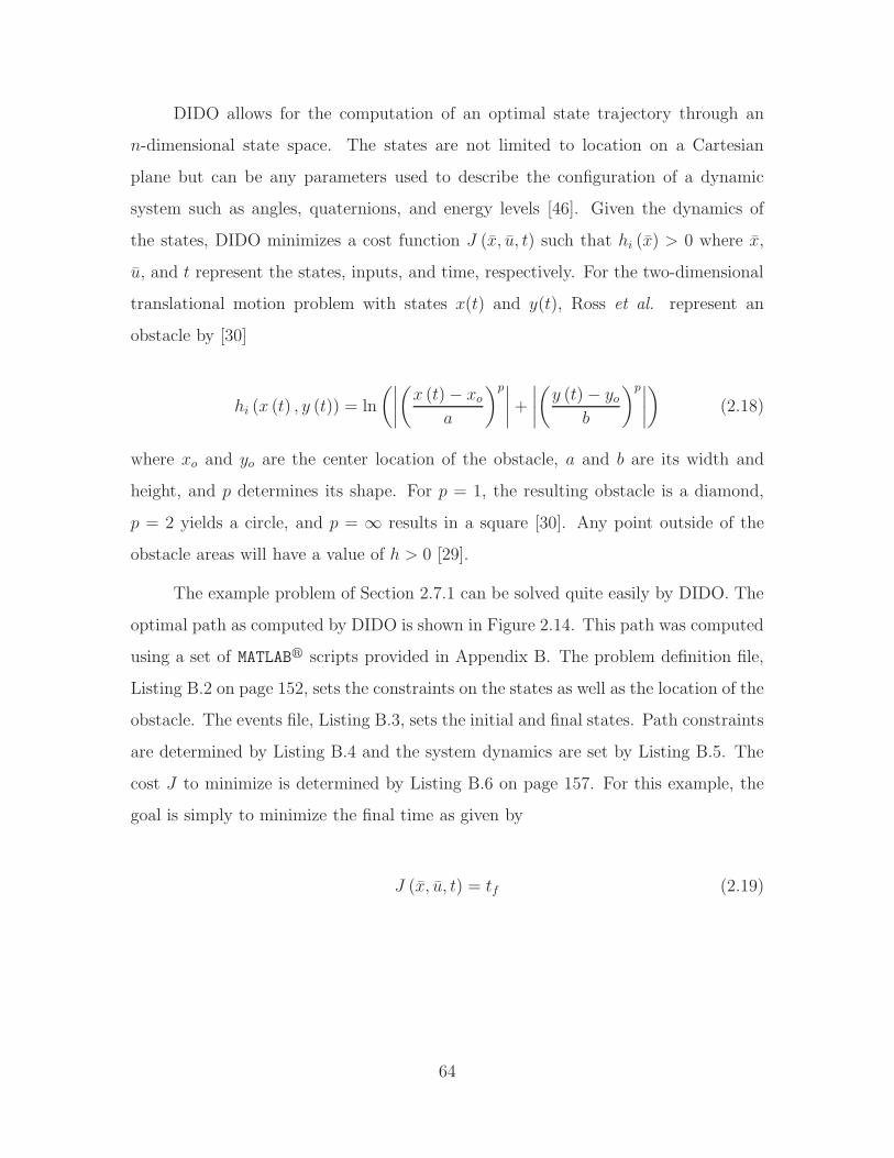
DIDO allows for the computation of an optimal state trajectory through an

n-dimensional state space. The states are not limited to location on a Cartesian

plane but can be any parameters used to describe the configuration of a dynamic

system such as angles, quaternions, and energy levels [46]. Given the dynamics of

the states, DIDO minimizes a cost function J (x, u, t) such that hi (x) > 0 where x,

u, and t represent the states, inputs, and time, respectively. For the two-dimensional

translational motion problem with states x(t) and y(t), Ross et al. represent an

obstacle by [30]

hi (x (t) , y (t)) = ln

(∣

∣

∣

∣

(

x (t) − xo

a

)p∣∣

∣

∣

+

∣

∣

∣

∣

(

y (t) − yo

b

)p∣∣

∣

∣

)

(2.18)

where xo and yo are the center location of the obstacle, a and b are its width and

height, and p determines its shape. For p = 1, the resulting obstacle is a diamond,

p = 2 yields a circle, and p = ∞ results in a square [30]. Any point outside of the

obstacle areas will have a value of h > 0 [29].

The example problem of Section 2.7.1 can be solved quite easily by DIDO. The

optimal path as computed by DIDO is shown in Figure 2.14. This path was computed

using a set of MATLABr scripts provided in Appendix B. The problem definition file,

Listing B.2 on page 152, sets the constraints on the states as well as the location of the

obstacle. The events file, Listing B.3, sets the initial and final states. Path constraints

are determined by Listing B.4 and the system dynamics are set by Listing B.5. The

cost J to minimize is determined by Listing B.6 on page 157. For this example, the

goal is simply to minimize the final time as given by

J (x, u, t) = tf (2.19)

64

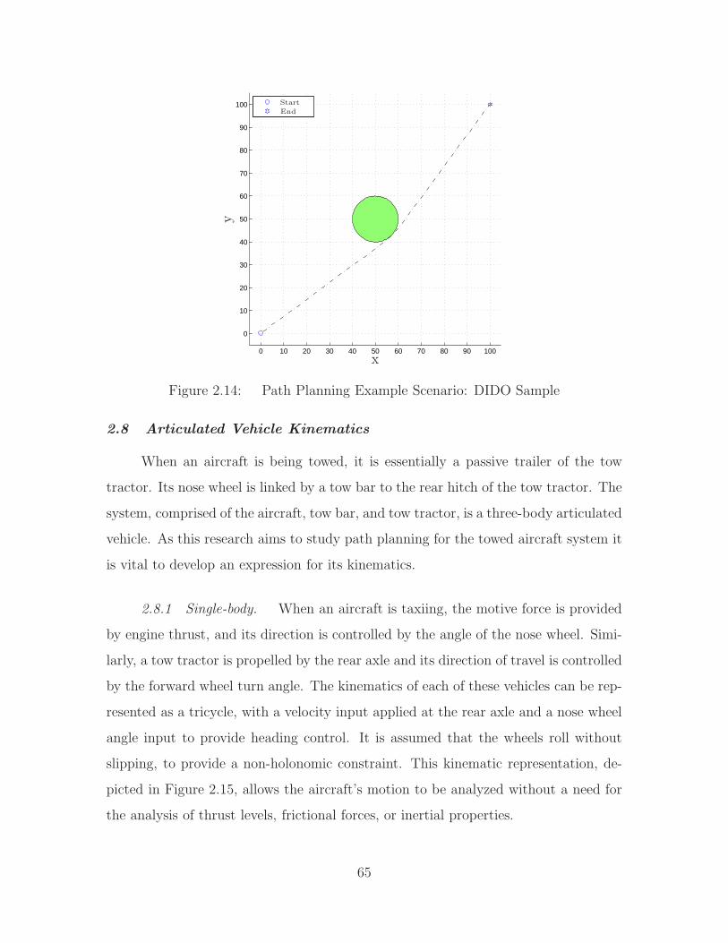
0 10 20 30 40 50 60 70 80 90 100

0

10

20

30

40

50

60

70

80

90

100

x

y

Start

End

Figure 2.14: Path Planning Example Scenario: DIDO Sample

2.8 Articulated Vehicle Kinematics

When an aircraft is being towed, it is essentially a passive trailer of the tow

tractor. Its nose wheel is linked by a tow bar to the rear hitch of the tow tractor. The

system, comprised of the aircraft, tow bar, and tow tractor, is a three-body articulated

vehicle. As this research aims to study path planning for the towed aircraft system it

is vital to develop an expression for its kinematics.

2.8.1 Single-body. When an aircraft is taxiing, the motive force is provided

by engine thrust, and its direction is controlled by the angle of the nose wheel. Simi-

larly, a tow tractor is propelled by the rear axle and its direction of travel is controlled

by the forward wheel turn angle. The kinematics of each of these vehicles can be rep-

resented as a tricycle, with a velocity input applied at the rear axle and a nose wheel

angle input to provide heading control. It is assumed that the wheels roll without

slipping, to provide a non-holonomic constraint. This kinematic representation, de-

picted in Figure 2.15, allows the aircraft’s motion to be analyzed without a need for

the analysis of thrust levels, frictional forces, or inertial properties.

65

ψ

xa

ya

φ

la

va

Figure 2.15: Moving Aircraft Free Body Diagram

The aircraft’s ground kinematics can be represented by the set of first order,

nonlinear differential equations

xa = va cosψ

ya = va sinψ (2.20)

ψ =va

latanφ

where φ is the steering angle of the nose wheel relative to the heading angle ψ, la is

the aircraft wheel base length, and va is the velocity of the aircraft.

When an aircraft is being towed, the input force is not being applied to the

aircraft’s center, but is instead applied at the nose wheel. This makes the aircraft the

trailing member of an articulated vehicle, much like a trailer being pulled by a truck.

The location of the nose wheel (xw, yw) is calculated by

(xw, yw) = (xa + la cosψ, ya + la sinψ) (2.21)

66

and if a velocity vw is applied at the nose wheel, then the resulting aircraft velocity

can be found by

va = vw cosφ. (2.22)

The aircraft kinematics given an input velocity at the nose wheel are given by

xa = va cosψ

ya = va sinψ (2.23)

ψ =vw

lasin φ.

2.8.2 Multi-body. The study of the control of articulated vehicles requires

an understanding of their kinematics. There are numerous areas of research utilizing

articulated vehicle kinematics. Ng et al. propose a vehicle following system utilizing a

virtual trailer link [36]. Bolzern et al. have performed extensive studies of articulated

vehicles with off-axle hitching [3] and n-body articulated vehicles [2] where the inde-

pendent variable is distance traveled. Larsson et al. propose a nonlinear state space

representation of a two-body system (a tractor and one trailer) [27]. The two-body

system is insufficient to represent the towed aircraft system ashore, as a tow bar is

used. Onboard an aircraft carrier, towing is often performed by a tow tractor which

attaches directly to the nose wheel creating a two-body system.

Park et al. propose a kinematic representation of an n-body articulated vehicle

with time as the independent variable [41]. Utilizing and adapting this representation

allows for the development of kinematics to represent the three-body articulated towed

aircraft system as shown in Figure 2.16.

The kinematics of the three-body articulated towed aircraft system can be devel-

oped by combining the single-body kinematics of each component. Given the forward

67

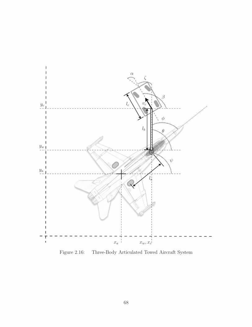
ψ

xa

ya

φ

la

vc

θlb

xw, xc

yw

yc

β

ζ

lc

α

Figure 2.16: Three-Body Articulated Towed Aircraft System

68

velocity of the tow tractor vc5 applied at its rear axle and the steering angle of the

front wheels α as the system inputs, the tow tractor’s motion can be described by

xc = vc cos β

yc = vc sin β (2.24)

β =vc

lctanα

where (xc, yc) gives the location of the tow tractor, β is the heading of the tow tractor

measured from the x-axis, and lc is the length of the tow tractor’s wheel base.

The tow bar, attached to the tow tractor’s rear hitch, is the first passive vehicle

in the three-body articulated towed aircraft system. As this research is concerned with

only simulating the towed aircraft system, for simplification it is assumed that the

tow tractor’s rear hitch is at the center of the rear axle. To attempt dynamic control

of a towed aircraft system, it should be modeled with off-axle hitching which is fairly

straightforward to accomplish [3]. With the tow bar hitched to the tow tractor’s rear

axle, the tow bar’s input velocity vc, and the tow bar steering angle ζ the velocity at

the nose wheel vw is given by

vw = vc cos ζ (2.25)

where vw is aligned with the direction angle of the tow bar θ and the nose wheels are

assumed to rotate or translate without slipping. The tow bar’s kinematics are then

described by

xw = vw cos θ

yw = vw sin θ (2.26)

θ =vc

lbsin ζ.

5The subscript c is utilized to denote cart.

69

where θ is the heading of the tow bar measured from the x-axis and lb is the length

of the tow bar. Combining the towed aircraft kinematics of Equation 2.23, the tow

bar kinematics of Equation 2.26, and the tow tractor kinematics of Equation 2.24 it

is straightforward to describe the motion of the three-body articulated towed aircraft

system by

x =

xc

yc

β

xw

yw

θ

xa

ya

ψ

,d

dtx =

d

dt

xc

yc

β

xw

yw

θ

xa

ya

ψ

=

vc cos β

vc sin β

vc

lctanα

vw cos θ

vw sin θ

vc

lbsin ζ

va cosψ

va sinψ

vw

lasinφ

, and u =

vc

α

(2.27)

where x is the state vector, u is the input vector, and

ζ = β − θ

φ = θ − ψ. (2.28)

It is also desired to implement some physical constraints of the towed aircraft

system. The tow bar can only rotate about the tow tractor’s hitch so far before it

collides with the tow tractor’s structure. Similarly, the structure of the aircraft’s

nose wheel places a constraint on its maximum rotation angle. DIDO is capable of

enforcing bounds on parameters, but it requires that they be represented as states.

The heading of each element of the towed aircraft system should also be able to make

70

as many complete revolutions, in either direction, as the path requires. Representing

the headings simply as angles will force DIDO to “unwind” the headings if they are

a full rotation from the goal. To enable this, the headings can be represented by two

states containing the sin and cos of the angle. The nonlinear kinematics are then

given by

d

dtx =

d

dt

xc

yc

sin β

cos β

xw

yw

sin θ

cos θ

ζ

xa

ya

sinψ

cosψ

φ

=

vc cos β

vc sin β

cos (β) β

− sin (β) β

vw cos θ

vw sin θ

cos (θ) θ

− sin (θ) θ

β − θ

va cosψ

va sinψ

cos (ψ) ψ

− sin (ψ) ψ

θ − ψ

=

vc cos β

vc sin β

cos (β) vc tan αlc

− sin (β) vc tan αlc

vc cos ζ cos θ

vc cos ζ sin θ

cos (θ) vc sin ζ

lb

− sin (θ) vc sin ζ

lb

β − θ

vc cos ζ cosφ cosψ

vc cos ζ cos φ sinψ

cos (ψ) vc cos ζ sinφ

la

− sin (ψ) vc cos ζ sin φ

la

θ − ψ

, and u =

vc

α

.

(2.29)

These equations could enable a persistent monitoring system to propagate the

motion of a towed aircraft forward in time based upon the measured locations and

orientations of the vehicles involved. They can also be used with DIDO, providing the

dynamics upon which to plan the optimal path to the desired position on the flight

deck.

71

2.9 Aircraft Tow Procedures

Towing aircraft on the flight deck or hangar bay of an aircraft carrier is a care-

fully planned procedure with standardized practices outlined by the CV NATOPS

Instruction (00-80t-120) [6]. This instruction calls for the following minimum person-

nel when towing an aircraft:

1. Director

2. Tractor Driver

3. Plane Captain

4. Two Plane Handlers

5. Two Wing Safeties (when required)

6. Tail Safety (when required)

For a fixed-wing aircraft, such as an FA-18C Hornet, this means that nine

personnel are required to move the aircraft. The Director is responsible for the entire

procedure. The Plane Captain provides braking control for the aircraft. The Plane

Handlers insert the chocks whenever the aircraft is at rest6. The Wing and Tail

Safeties walk in a fixed position relative to the wingtip or tail to ensure that no

collisions occur in that area [6].

The Director is required to maintain visual contact with the Plane Captain at

all times and all personnel are equipped with whistles, which they must hold in their

mouths, to signal each other [6].

6The Plane Handler and Wing Safety roles are typically fulfilled by the same personnel whenashore.

72

III. Data Collection

This chapter describes a series of tests conducted at the Air Force Institute of

Technology (AFIT) and Naval Air Station (NAS) Oceana designed to determine

if position and velocity measurements provided by the Global Positioning System

(GPS) are capable of supporting a system to monitor the position, orientation, and

velocity of aircraft, equipment, and personnel on the flight deck of a U.S. Navy aircraft

carrier. The equipment used in these tests is also described.

3.1 AFIT Tests

This section describes the tests conducted at AFIT. These tests were performed

to gain experience using the hardware, analyzing the collected data prior to testing

with aircraft, and to provide the data necessary to create and evaluate simulations.

Conducting these tests at AFIT allowed for an estimate of the requirements and risks

associated with the tests, prior to performing them with actual aircraft.

3.1.1 Vehicle Measurements. The first test was designed to determine the

position and orientation of a small vehicle using two GPS receivers. From the recorded

GPS data, the geometry of the vehicle, and the location of each receiver on the vehicle,

the position of the vehicle and its orientation can be calculated.

The goal of this test was to determine the level of precision that can be achieved

in the position and orientation calculations and to observe the effect of measurement

noise of the resulting calculations. Additionally, the software written to analyze the

recorded data can be used again with data recorded at NAS Oceana. Figure 3.1

illustrates the notional setup of this test.

3.1.1.1 Requirements. The following equipment was required for this

test:

1. Golf cart

2. Mobile GPS recorders (quantity: 2)

73

GPS Recorder

GPS Recorder

Vehicle

x

y

ψ

Figure 3.1: Notional Setup of AFIT Vehicle Measurements Test

3. Dual-frequency GPS antenna (quantity: 2)

4. Stationary GPS recorder

The GPS recorders were attached to right and left side of the golf cart with

the antennae supported away from the body of the golf cart. The stationary GPS

recorder measured the position of the AFIT Advanced Navigation Technology (ANT)

center roof antenna for differential corrections.

3.1.1.2 Procedure. This test was conducted in two phases. The first

phase, static measurements, tests the accuracy and precision of the recorders’ mea-

surements while at rest. The second phase, dynamic measurements, tests the recorders

while in motion.

For static measurements, the vehicle was kept in a parked position for at least

five minutes. The dynamic phase involved driving the vehicle around the field behind

AFIT at a walking pace in straight lines or smooth curves. The recorded data can

74

Personnel

GPS Recorder

Vehicle

Simulated Aircraft

Figure 3.2: Vehicle and Personnel Simulating Aircraft Movement

be used to analyze the noise in the measurement signal and the ability of software to

predict the path of the vehicle.

3.1.1.3 Expected Results. This test provides results for the accuracy

of the position (eg: ±2 cm) and orientation (eg: ±2 degrees) of the GPS data as well

as its precision (eg: ±1 cm 97% of time). Additionally, it should allow observation of

the effect of multipath error on measurements.

3.1.2 Vehicle and Personnel Movement. This test recorded the movements

of both the vehicle used in Section 3.1.1 and personnel simultaneously. It was de-

signed to simulate the towing of an aircraft with its required personnel, allowing the

development of analysis software prior to conducting the test in Section 3.2.1. Fig-

ure 3.2 illustrates the configuration for this test. Images recorded from the test are

provided in Figure 3.3.

75

Figure 3.3: Photographs from Simulated Aircraft Move at AFIT

3.1.2.1 Requirements. The following equipment was required for this

test:

1. Golf cart

2. Helmet (quantity: 4)

3. Backpack (quantity: 4)

4. Mobile GPS recorder (quantity: 6)

5. Stationary GPS recorder

6. Dual-frequency GPS antenna (quantity: 6)

The golf cart was configured with two mobile GPS recorders as in Section 3.1.1.1.

The backpacks, helmets, and remaining mobile GPS recorders were carried by per-

sonnel wearing the helmets with dual-frequency antenna attached. This test required

four personnel to walk with the vehicle, all volunteers were AFIT students or faculty.

76

3.1.2.2 Procedure. For this test the golf cart was driven slowly along a

path behind AFIT. The personnel walked with the cart in an imitation of an aircraft

movement crew, as depicted in Figure 3.2.

3.1.2.3 Expected Results. From the data collected in this simulation,

software was developed which will be used to analyze the data collected at NAS

Oceana, described in Section 3.2.1.

3.2 NAS Oceana Tests

The tests to be performed at NAS Oceana build upon those described in Sec-

tion 3.1. The purpose is to observe the movement of U.S. Naval aircraft and sailors as

they perform tasks similar to those performed on the flight deck of an aircraft carrier.

By observing these tasks, a better understanding of the motion of aircraft, equip-

ment, and personnel on the flight deck can be gained. These tests were conducted

at a shore installation, but the differences in aircraft handling between sea and shore

are minimal.

Collecting data with aircraft presents a greater risk than the simpler tests con-

ducted at AFIT. Even without power being applied to the aircraft, it is vital that

proper flight line procedures be observed for the safety of both the aircraft, SE, and

personnel involved.

The Naval Aviation Maintenance Program (NAMP) [5] requires that tools used

on aircraft be accounted for at all times. This is done to prevent Foreign Object

Damage (FOD) from occurring to aircraft or personnel. During these tests, AFIT

property was placed temporarily on and around Naval aircraft and personnel. All

equipment used for this test was therefore inspected before and after each test to

ensure that no parts, such as nuts or bolts, were lost during testing.

3.2.1 Aircraft Towing Observation. This test recorded the position, orienta-

tion, and velocity of an aircraft as it was towed from one spot to another on the NAS

77

Oceana flight line as well as the position and velocity of the personnel required for the

towing. This procedure is virtually identical to that performed onboard an aircraft

carrier. Figure 3.4 illustrates the towing procedure to be observed. A photograph of

the test being conducted is presented in Figure 3.5 depicting the antennae mounted

on USN cranials1 and wingtip mounted GPS recorders.

The purpose of this test was to gather data which fully describes the motion of

an aircraft being towed and the personnel around it. This data can then be analyzed

for a better understanding of flight deck operations and used in simulations for hazard

prediction and UAV incorporation.

3.2.1.1 Requirements. The following equipment was required for this

test:

1. Cranial (quantity: 6)

2. Backpack (quantity: 6)

3. Nylon GPS recorder pouch (quantity: 2)

4. Mobile GPS recorders (quantity: 8)

5. Stationary GPS recorder

6. Dual-frequency GPS antenna (quantity: 9)

7. Video camera (quantity: 2)

8. Aircraft (quantity: 1)

9. Tow Tractor and bar

10. Elevated support platform (B-1 stand)

11. Laptop computer

1Cranial is the term used to describe the helmet used in Naval Aviation which contains hearingand vision protection.

78

Personnel

End Point

Start Point

GPS Recorders

Tow Tractor

Figure 3.4: Example Aircraft Tow Plan

Figure 3.5: Photograph of Aircraft Being Towed at NAS Oceana

79

Two mobile GPS recorders were affixed on the wingtips of the aircraft using the

nylon pouches made by squadron personnel, depicted in Figure 3.6. This mounting

was designed to be completely non-permanent involving no modification to the aircraft

or metal on metal contact.

The remaining mobile GPS recorders were provided to the tow personnel to

record their movements with cranial mounted antennae and backpacks. The Plane

Captain in the cockpit was not provided with a GPS recorder as their position was

fixed relative to the aircraft during the entire procedure. The Tow Tractor and bar

was used to move the aircraft. A video record of the test was made with a video

camera placed atop the elevated support platform and another was used at ground

level.

The stationary GPS recorder was used to record data for differential correction

in post-processing. It was placed near the flight line atop the elevated support plat-

form. The laptop computer was used to store the recorded data after each portion of

the test.

A sufficient number of trained USN personnel were needed to perform the towing

procedure. NAS Oceana instructions require a minimum of six trained personnel to

tow an aircraft. The squadron’s maintenance department provided a sufficient number

of qualified volunteers to perform the tow procedure.

3.2.1.2 Procedure. After mounting the GPS recorders as described in

Section 3.2.1.1, the aircraft was towed from one spot to another on the flight line,

similar to the tow plan depicted in Figure 3.4. The tow personnel were directed to

park the aircraft multiple times, with both forward and reverse motion. This test

was conducted with two different groups of personnel: one group during the day, the

other at night.

3.2.1.3 Expected Results. The data provided by this test allows a

more thorough understanding of the movement of aircraft, equipment, and personnel

80

Figure 3.6: Nylon Pouch Made for Leica Recorder With Antenna Mount: Nylonwebbing with velcro bands was used to lash the recorder to aircraft wingtip pylons.Pouches were made and provided by sailors of Strike Fighter Squadron Three Four -The Blue Blasters.

81

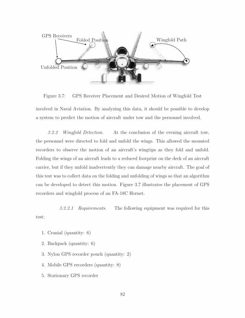
GPS Receivers

Unfolded Position

Folded Position Wingfold Path

Figure 3.7: GPS Receiver Placement and Desired Motion of Wingfold Test

involved in Naval Aviation. By analyzing this data, it should be possible to develop

a system to predict the motion of aircraft under tow and the personnel involved.

3.2.2 Wingfold Detection. At the conclusion of the evening aircraft tow,

the personnel were directed to fold and unfold the wings. This allowed the mounted

recorders to observe the motion of an aircraft’s wingtips as they fold and unfold.

Folding the wings of an aircraft leads to a reduced footprint on the deck of an aircraft

carrier, but if they unfold inadvertently they can damage nearby aircraft. The goal of

this test was to collect data on the folding and unfolding of wings so that an algorithm

can be developed to detect this motion. Figure 3.7 illustrates the placement of GPS

recorders and wingfold process of an FA-18C Hornet.

3.2.2.1 Requirements. The following equipment was required for this

test:

1. Cranial (quantity: 6)

2. Backpack (quantity: 6)

3. Nylon GPS recorder pouch (quantity: 2)

4. Mobile GPS recorders (quantity: 8)

5. Stationary GPS recorder

82

6. Dual-frequency GPS antenna (quantity: 9)

7. Video camera

8. Aircraft (quantity: 1)

9. Speed Handles (quantity: 2)

10. Laptop computer

Two mobile GPS recorders were affixed to the wingtip of an aircraft in the

same manner described in Section 3.2.1.1. The stationary GPS recorder was used for

differential correction. The laptop computer was used to record the data from the

receivers. A visual record of the test was made with the video camera. Speed handles

were used to manually fold and unfold the wings.

3.2.2.2 Procedure. This test was started with the wings in the unfolded

position at the conclusion of the evening aircraft tow procedure. Personnel on either

side of the aircraft were directed to use the speed handles to fold and then unfold the

wings. Following the test, the GPS recorders were removed from the wingtips, and

the aircraft was returned to its normal parking configuration.

3.2.2.3 Expected Results. Analysis of the data collected in this test

helps in the development of an algorithm to detect a change in the wingfold status of

an aircraft.

3.2.3 Personnel Tracking Near Aircraft. During flight operations on an

aircraft carrier, it is routine for authorized personnel to approach a powered aircraft

quickly and remain in close proximity. This test explores the ability of GPS position

data to monitor such motion of personnel. The motion of personnel near an aircraft

and the hazardous areas near it is depicted by Figure 3.8. The preparations made to

tow an aircraft provide many opportunities to record the motion of personnel near

the aircraft.

83

Path

Personnel

Simulated “Hazard” Area

Figure 3.8: Tracking Personnel Near an Aircraft

3.2.3.1 Requirements. The following equipment was required for this

test:

1. Cranial (quantity: 6)

2. Backpack (quantity: 6)

3. Nylon GPS recorder pouch (quantity: 2)

4. Mobile GPS recorders (quantity: 8)

5. Stationary GPS recorder

6. Dual-frequency GPS antenna (quantity: 9)

7. Video camera (quantity: 2)

8. Aircraft (quantity: 1)

9. Tow cart and bar

10. Elevated support platform (B-1 stand)

11. Laptop computer

Six mobile GPS recorders were carried by personnel, as in Section 3.1.2, who

were involved in the aircraft tow procedure. Two mobile GPS recorders were affixed

to the aircraft wingtips. A stationary GPS recorder was used to collect data for

84

differential correction. The video camera was used to create a visual record of the

test. The computer was used to collect data from the GPS receivers.

3.2.3.2 Procedure. Throughout the test described in Section 3.2.1,

it was often necessary for the personnel involved to approach the aircraft closely.

The recorded data in these situations allows the simulation of maintenance personnel

approaching hazard areas, such as the engine intake and exhaust.

3.2.3.3 Expected Results. As maintenance personnel often get very

near aircraft, even crawl underneath them, during pre-launch procedures it is expected

that the accuracy of the GPS solution will degrade significantly due to the effect of

multipath and other factors. At times, the GPS receivers may even lose lock and be

unable to compute a solution.

The final result of this test demonstrates the ability of small GPS receivers to

track the motion of personnel near aircraft on the flight deck of an aircraft carrier.

The algorithms developed from data collected in the test described by Section 3.1

should be able to determine if personnel enter the simulated engine “hazard” areas.

3.3 Equipment

This section describes the GPS equipment used during the tests of Sections 3.1

and 3.2.

3.3.1 Custom GPS Recorders. Two of the GPS recorders provided by the

ANT center, referred to as the Custom GPS Recorders, are comprised of a NovAtel

OEMV-3 card, a Gumstix computer, and a 12V lithium-polymer battery. They are

contained within an aluminum enclosure with power switch, status indicator light,

Ethernet port, and antenna jack as depicted in Figure 3.9.

The system is wired so that the NovAtel OEMV-3 and Gumstix computer are

both started when the switch is turned to the on position. The OEMV-3 takes

85

Figure 3.9: Diagram of Custom GPS Recorder

Figure 3.10: NovAtel OEMV-3

approximately five seconds to begin transmitting messages, while the computer takes

approximately 30 seconds to boot and run the logging software.

3.3.1.1 NovAtel OEMV-3. The NovAtel OEMV-3, depicted in Fig-

ure 3.10 [39, pg. 28] is a triple frequency GPS receiver capable of computing code and

carrier phase solutions as well as processing differential GPS error corrections. It can

utilize GPS signals broadcast on L1, L2, and the upcoming L5 as well as the Russian

GLONASS L1 and L2 signals. For these tests, it was configured to track only GPS

L1 and L2. It is capable of tracking 14 GPS satellites simultaneously. [39, p. 27].

For this research, the NovAtel OEMV-3 is configured to transmit satellite rang-

ing (RANGECMPA) and ephemeris (RAWEPHEMA) data as well as its best position

86

Table 3.1: NovAtel ASCII Message Header Format

Field Name Description

1 Sync “#” symbol starts every message.2 Message Type of message. For this

research only RANGECMPA,RAWEPHEMA, or BESTPOSA.

3 Port Communications port transmit-ted on. For this research onlyCOM2.

4 Sequence Number Used for multiple related logs.Normally 0.

5 Percent Idle Time Minimum percent of time proces-sor is idle between successive logs.

6 GPS Time Status Indicates the quality of GPS timesolution.

7 Week GPS Week Number.8 Seconds Seconds since start of GPS week.9 Receiver Status Eight digit hexadecimal number

reporting status of hardware/-software components.

10 Reserved Not described by NovAtel.11 Version Receiver software build number.12 ; Semi-colon describes end of mes-

sage header.

solution (BESTPOSA) to its second serial communications port (COM2). This infor-

mation is transmitted in an ASCII message, and is therefore directly human readable.

Each of the messages is transmitted with a header using the format described in Ta-

ble 3.1 [38, pg. 22].

Following the message header, the RANGECMPA, RAWEPHEMA, and BEST-

POSA message each contain different information. RANGECMPA contains hexadec-

imal information on the calculated range to each satellite, on each frequency the

receiver has acquired. RAWEPHEMA is an ephemeris message for each satellite the

receiver has acquired. BESTPOSA is the best possible position the receiver can cal-

87

Figure 3.11: Onboard Computer, Exploded View

culate from available data. RANGECMPA is transmitted at 5 Hz, BESTPOSA at 1

Hz, while RAWEPHEMA is transmitted every five minutes.

A description of the contents of each navigation message is provided by the

OEMV Family Firmware Reference Manual [38, pgs. 250, 401, 408].

3.3.1.2 Onboard Computer. The onboard computer runs an embed-

ded version of the Linux operating system. It executes the program provided in

Listing B.14 on page 178 to record the data transmitted by the NovAtel receiver on

COM2 to a file located on a removable MultiMediaCard (MMC) flash chip.

The motherboard is a Gumstix “Connex” series with a Marvellr PXA-255 400

MHz processor, 64 MB of RAM, and onboard Flash storage of 16 MB for the operating

system. It is configured with two daughterboards: a “breakout-gs” for serial commu-

nications and a “netMMC” for Ethernet and MMC connections. Figure 3.11 provides

an exploded view of the Gumstix computer and its daughterboard with Ethernet and

MMC connections [17].

It is possible to communicate with the onboard computer over its serial port

or its Ethernet port. When connecting over Ethernet, the computer is configured to

88

announce which remote connection services are running using the Network Zerconf

Protocol2 software. Conveniently, this means a computer connected to it can tell if its

remote connection processes are running. The Secure Shell3 allows for both a remote

terminal connection and copying of files over the network.

The computer is configured to boot the Linuxr OpenEmbedded operating sys-

tem from its onboard Flash storage. The startup scripts of the operating system have

been configured to execute the logging program of Listing B.14 at the conclusion of

the boot sequence.

The logging program runs from and only manipulates files on the MMC storage.

It first determines which run number it is on to create sequential file names for the

recorded data. It reads this data from run file.txt, and each receiver is configured to

start at a different number (1000, 2000).

3.3.2 Leica GX1210. The ANT center also provided six Leica GX1210 GPS

receivers. The default GX1210 is only capable of single frequency (L1) measurements,

but the six units owned by the AFIT ANT center have been upgraded to support dual

frequency (L1 and L2) measurements. They have 14 channels for each frequency.

There are two RX1200 controllers which attach to the GX1210 and provide a

touch-screen graphical user interface. Figure 3.12 shows a GX1210 with an attached

RX1200.

Measurements are stored to an internal 2 GB CompactFlash card. Technical

specifications claim 20 mm accuracy when differential corrections are applied in post-

processing. They are powered by up to two rechargeable Lithium Ion batteries (4.2

Ah / 7.4 V). One battery powers the receiver for approximately 30 hours.

2http://avahi.org3http://openssh.com

89

Figure 3.12: Leica GX1210 With RX1200 Interface

90

3.3.3 Antennae. Three different models of antenna were used during test-

ing at AFIT and NAS Oceana. Every antenna used was capable of dual-frequency

reception. During the NAS Oceana tests personnel were equipped with one of two

antennae: the ANT-A72GA-TW-N or the ANT-35C2GA-NW, both distributed by

NovAtel and manufactured by Antcom. The primary difference is the connector: the

former using a TNC connector and the latter a N-connector. The Leica recorders

mounted on the aircraft wingtips were equipped with a Leica AX1202 GG antenna,

also using a TNC connector.

91

IV. Results

This chapter describes the results of the tests conducted in Chapter III. The

AFIT tests were designed to demonstrate the capacity of mobile GPS recorders

mounted at fixed distances to allow the position and heading of a moving vehicle

to be calculated. Algorithms used to calculate the results are also explained in this

chapter. The NAS Oceana tests provide highly accurate measurements of procedures

very similar to those performed aboard U.S. Navy aircraft carriers. Results from the

tests at NAS Oceana include aircraft tow velocities (translational and rotational) as

well as the distance personnel maintain from the aircraft.

4.1 AFIT Test Results

This section provides the results of preliminary testing conducted at AFIT. The

performance differences between the Custom and Leica GPS recorders are discussed.

4.1.1 Test Vehicle Antenna Distance. With two GPS antennae mounted on

a rigid aluminum bar on the test vehicle, as described in Section 3.1.1 on page 73,

the first data collected was analyzed to determine the accuracy and precision of the

measurements. As an initial test, the two Custom GPS recorders were attached to

the test vehicle antennae. Figure 4.1 shows the distance between the antennae, made

using the BESTPOSA solution, for both static and kinematic regimes, provided by

the Custom GPS Recorders, described in Section 3.3.1 on page 85. The BESTPOSA

solution, referred to as a Single Point Solution (SPS), is calculated solely by the

receiver and does not include any differential corrections, so ephemeris and tropo-

spheric errors should be present. Additionally, without a base station present only

code phase measurements can be computed. The measured distance (using a tape

measure) between the antennae phase centers was 0.464 m.

When a third receiver was made available, the same two receivers were mounted

to the test vehicle but a stationary receiver was used to collect data for differential

correction. From this point forward the data collected in all tests has differential

92

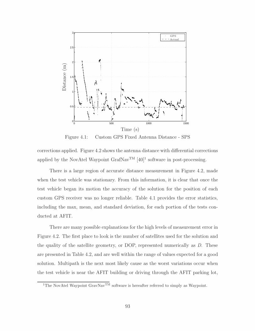
0 500 1000 15000

0.5

1

1.5

2

2.5

3

Time (s)

Dista

nce

(m)

GPS

Actual

Figure 4.1: Custom GPS Fixed Antenna Distance - SPS

corrections applied. Figure 4.2 shows the antenna distance with differential corrections

applied by the NovAtel Waypoint GrafNavTM [40]1 software in post-processing.

There is a large region of accurate distance measurement in Figure 4.2, made

when the test vehicle was stationary. From this information, it is clear that once the

test vehicle began its motion the accuracy of the solution for the position of each

custom GPS receiver was no longer reliable. Table 4.1 provides the error statistics,

including the max, mean, and standard deviation, for each portion of the tests con-

ducted at AFIT.

There are many possible explanations for the high levels of measurement error in

Figure 4.2. The first place to look is the number of satellites used for the solution and

the quality of the satellite geometry, or DOP, represented numerically as D. These

are presented in Table 4.2, and are well within the range of values expected for a good

solution. Multipath is the next most likely cause as the worst variations occur when

the test vehicle is near the AFIT building or driving through the AFIT parking lot,

1The NovAtel Waypoint GravNavTM software is hereafter referred to simply as Waypoint.

93

0 500 1000 1500 2000 2500 30000.446

0.448

0.45

0.452

0.454

0.456

0.458

0.46

0.462

0.464

0.466

Time (s)

Dista

nce

(m)

GPSActual

(a) Static Regime

2700 2800 2900 3000 3100 3200 3300 3400 3500 36000

2

4

6

8

10

12

14

Time (s)

Dista

nce

(m)

GPSActual

(b) Kinematic Regime

Figure 4.2: Custom GPS Fixed Antenna Distance - CDGPS

both being highly reflective areas. This is an unlikely cause as multipath error should

be fairly random, and in a video playback of the recorded data the measurement

errors are consistently in the direction of motion. Another possibility considered was

that the NovAtel OEMV receivers were changing which satellites were used in the

solution during the kinematic phase, a common practice for receivers with a small

number of channels. This possibility was discarded as the OEMV has 14 channels

on each frequency which is more than sufficient for the number of available satellites.

Additionally, the determination of which satellites to use in the solution is performed

by Waypoint during post-processing, which should eliminate discontinuities.

Another possibility, inherent to the receiver construction and not the calcula-

tion of the solution, is a constraint in available bandwidth in the system bus linking

the MMC card and the serial port. While the serial port was capable of handling

RANGECMPA message at 5 Hz, BESTPOSA messages at 1 Hz, the bursting of

RAWEPHEMA every five minutes may have overloaded the bus and caused ephemeris

messages to be lost. This does not appear to be the case, as valid solutions are ob-

tained with multiple satellites as depicted in Table 4.2, but it should be left open as

a possibility.

94

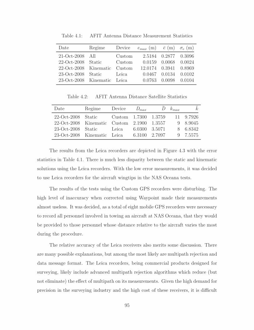
Table 4.1: AFIT Antenna Distance Measurement Statistics

Date Regime Device emax (m) e (m) σe (m)

21-Oct-2008 All Custom 2.5184 0.2877 0.309622-Oct-2008 Static Custom 0.0159 0.0068 0.002422-Oct-2008 Kinematic Custom 12.0174 0.3941 0.896923-Oct-2008 Static Leica 0.0467 0.0134 0.010223-Oct-2008 Kinematic Leica 0.0763 0.0098 0.0104

Table 4.2: AFIT Antenna Distance Satellite Statistics

Date Regime Device Dmax D kmax k

22-Oct-2008 Static Custom 1.7300 1.3759 11 9.792622-Oct-2008 Kinematic Custom 2.1900 1.3557 9 8.904523-Oct-2008 Static Leica 6.0300 3.5071 8 6.834223-Oct-2008 Kinematic Leica 6.3100 2.7097 9 7.5575

The results from the Leica recorders are depicted in Figure 4.3 with the error

statistics in Table 4.1. There is much less disparity between the static and kinematic

solutions using the Leica recorders. With the low error measurements, it was decided

to use Leica recorders for the aircraft wingtips in the NAS Oceana tests.

The results of the tests using the Custom GPS recorders were disturbing. The

high level of inaccuracy when corrected using Waypoint made their measurements

almost useless. It was decided, as a total of eight mobile GPS recorders were necessary

to record all personnel involved in towing an aircraft at NAS Oceana, that they would

be provided to those personnel whose distance relative to the aircraft varies the most

during the procedure.

The relative accuracy of the Leica receivers also merits some discussion. There

are many possible explanations, but among the most likely are multipath rejection and

data message format. The Leica recorders, being commercial products designed for

surveying, likely include advanced multipath rejection algorithms which reduce (but

not eliminate) the effect of multipath on its measurements. Given the high demand for

precision in the surveying industry and the high cost of these receivers, it is difficult

95

0 200 400 600 800 1000 1200 1400 1600 1800 20000.43

0.44

0.45

0.46

0.47

0.48

0.49

0.5

0.51

0.52

Time (s)

Dista

nce

(m)

GPSActual

(a) Static Regime

1900 2000 2100 2200 2300 2400 2500 26000.38

0.4

0.42

0.44

0.46

0.48

0.5

0.52

Time (s)

Dista

nce

(m)

GPSActual

(b) Kinematic Regime

Figure 4.3: Leica Fixed Antenna Distance - CDGPS

to imagine multipath rejection is not incorporated. Another possible explanation is

the use of a binary message format, alleviating the bandwidth concerns. The ASCII

message used by the NovAtel receivers is a relatively inefficient method of transmitting

the measurement data.

4.1.2 Test Vehicle Heading. The heading of the test vehicle is calculated

using the equations derived in Section 2.5 on page 52. The MATLABr script created to

perform this calculation is provided as Listing B.7 in Appendix B on page 158. The

MATLABr command atan2 is used to provide quadrant resolution when determining

the heading.

Considering the inaccuracy of the position measurements from the Custom GPS

recorders, it was expected that the heading calculation would contain significant levels

of noise, making it unusable for proper attitude determination. As seen in Figure 4.4,

the actual heading is virtually impossible to determine at any given time due to

the rapid fluctuations. When the same calculations are performed using the Leica

recorders the results contain significantly less noise. This allows the heading at any

given moment to be accurately measured. In fact, using the Leica recorders allows

the turns taken by the test vehicle to be clearly identified.

96

0 500 1000 1500 2000 2500 3000−97.2

−97

−96.8

−96.6

−96.4

−96.2

−96

−95.8

Time (s)

Hea

din

g(d

eg)

(a) Static Regime - Custom GPS Recorder

2700 2800 2900 3000 3100 3200 3300 3400 3500 3600−200

−150

−100

−50

0

50

100

150

200

Time (s)

Hea

din

g(d

eg)

(b) Kinematic Regime - Custom GPS Recorder

0 200 400 600 800 1000 1200 1400 1600 1800 200076

78

80

82

84

86

88

Time (s)

Hea

din

g(d

eg)

(c) Static Regime - Leica Recorder

1900 2000 2100 2200 2300 2400 2500 2600−200

−150

−100

−50

0

50

100

150

200

Time (s)

Hea

din

g(d

eg)

(d) Kinematic Regime - Leica Recorder

Figure 4.4: AFIT Test Vehicle Heading

97

4.2 NAS Oceana Test Results

This section describes the results of the tests conducted at NAS Oceana, VA.

Topics include the measurement of aircraft wingspan b, calculation of position (xa, ya)

and heading ψ, and the path along which the aircraft was towed.

4.2.1 Aircraft Wingspan. The two Leica recorders mounted on the wingtips

provide an excellent indicator of the accuracy and precision of the GPS solution.

The recorders were strapped to the inboard side of the wingtip missile pylons using

the nylon pouches made by squadron personnel depicted in Figure 3.6 on page 81.

The distance between these pylons is fixed when the wings are spread, so the only

variation should result from the placement of the recorders along the length of the

pylon. According to Jane’s All the World’s Aircraft, the wingspan of an FA-18C

Hornet is b = 11.43 m [23].

Figure 4.5 shows the wingspan measurements taken during the morning and

evening tow procedures. Of note is the increased noise level in the latter phase of the

evening test. In this portion, the wingspan measurement varies about the actual, but

does approach it. The difference in distance measurements may also be attributable

to the location of the phase center of the antennae.

The morning and evening wingspan error statistics are provided in Table 4.3.

There are many factors which may explain the increased error during the evening

portion, but the most likely explanation is increased multipath due to the increased

number of aircraft on the flight line. During the day portion, there were approximately

four total aircraft on the area of flight line used. Twice that number were present

during the evening portion.

4.2.2 Aircraft Heading and Heading Rate. The heading of the aircraft ψ

is determined by the same algorithm as the AFIT test vehicle, with the MATLABr

script provided in Listing B.7 on page 158. To determine the heading rate, it was

necessary to numerically differentiate the calculated heading data, a process which

98

0 200 400 600 800 1000 1200 1400 1600 1800

11.4

11.45

11.5

11.55

11.6

11.65

11.7

Time (s)

Win

gspan

b(m

)

GPS

Actual

(a) Morning

0 200 400 600 800 1000 120010.4

10.6

10.8

11

11.2

11.4

11.6

11.8

12

Time (s)

Win

gspan

b(m

)

GPS

Actual

(b) Evening

Figure 4.5: NAS Oceana Aircraft Wingspan Measurements

99

Table 4.3: NAS Oceana Aircraft Wingspan Measurement Statistics

Time emax (m) e (m) σe (m)

Morning 0.1842 0.0535 0.0140Evening 0.9808 0.1333 0.1727

often introduces noise into measurements. The diff command, included with MATLABr

was used for the heading rate calculation and the resulting array was padded with

a leading zero to maintain array length. Since the aircraft was initially at rest this

leading zero does not affect the results.

One potentially useful element of information that can be derived from the

observation of an aircraft tow procedure is the maximum turn rate used. This can

be used to provide a motion planning algorithm with more realistic estimates of the

vehicle capabilities. The maximum turn rate is a function of the nose wheel angle

and the maximum tow cart velocity. While the maximum turn rate used in these

tests ashore may not be the maximum capable, it should be on the same order of

magnitude. The heading and heading rate of the tow procedure conducted at NAS

Oceana are provided in Figure 4.6.

By calculating the heading rate of an aircraft, it would be possible to predict

the change of hazard areas with time. As an example, the motion of the area behind

a taxiing aircraft containing hazardous exhaust can be predicted. If the hazard area

will intersect a sailor within a short time horizon, a warning could be issued to the

sailor and pilot.

4.2.3 Aircraft Position and Velocity. Analyzing the route taken with the

towed aircraft allows for analysis of safe distances between aircraft (ashore) and route

preferences. Figure 4.7 shows the path taken for both morning and evening tow

procedures. It is clear from this data that there are set routes between the rows of

aircraft parking spaces, and that during this test two of them were used. There were

in fact painted taxiway markings on the flight line which were used between rows of

100

0 200 400 600 800 1000 1200 1400 1600 1800−200

−100

0

100

200

0 200 400 600 800 1000 1200 1400 1600 1800−10

−5

0

5

10

Time (s)

Hea

din

gψ

(deg

)H

eadin

gR

ateψ

(deg

/s)

(a) Morning

0 200 400 600 800 1000 1200−150

−100

−50

0

50

100

150

0 200 400 600 800 1000 1200−30

−20

−10

0

10

20

Time (s)

Hea

din

gψ

(deg

)H

eadin

gR

ateψ

(deg

/s)

(b) Evening

Figure 4.6: NAS Oceana Towed Aircraft Heading and Heading Rate

101

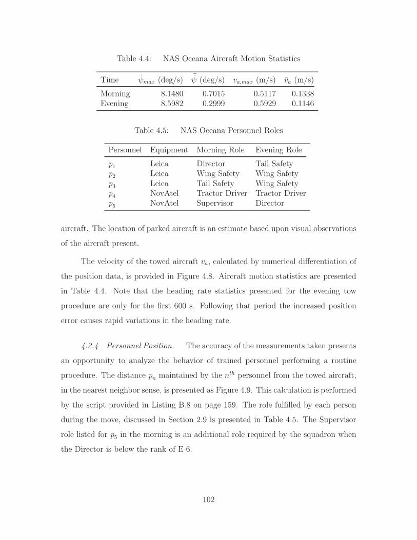
Table 4.4: NAS Oceana Aircraft Motion Statistics

Time ψmax (deg/s) ¯ψ (deg/s) va,max (m/s) va (m/s)

Morning 8.1480 0.7015 0.5117 0.1338Evening 8.5982 0.2999 0.5929 0.1146

Table 4.5: NAS Oceana Personnel Roles

Personnel Equipment Morning Role Evening Role

p1 Leica Director Tail Safetyp2 Leica Wing Safety Wing Safetyp3 Leica Tail Safety Wing Safetyp4 NovAtel Tractor Driver Tractor Driverp5 NovAtel Supervisor Director

aircraft. The location of parked aircraft is an estimate based upon visual observations

of the aircraft present.

The velocity of the towed aircraft va, calculated by numerical differentiation of

the position data, is provided in Figure 4.8. Aircraft motion statistics are presented

in Table 4.4. Note that the heading rate statistics presented for the evening tow

procedure are only for the first 600 s. Following that period the increased position

error causes rapid variations in the heading rate.

4.2.4 Personnel Position. The accuracy of the measurements taken presents

an opportunity to analyze the behavior of trained personnel performing a routine

procedure. The distance pn maintained by the nth personnel from the towed aircraft,

in the nearest neighbor sense, is presented as Figure 4.9. This calculation is performed

by the script provided in Listing B.8 on page 159. The role fulfilled by each person

during the move, discussed in Section 2.9 is presented in Table 4.5. The Supervisor

role listed for p5 in the morning is an additional role required by the squadron when

the Director is below the rank of E-6.

102

0 20 40 60 80 100 120 140 160 180−20

0

20

40

60

80

100

120

140

Easting (m)

Nor

thin

g(m

)Initial Position

Final Position

Parked AircraftParked Aircraft

(a) Morning

0 20 40 60 80 100 120 140 160 180−20

0

20

40

60

80

100

120

140

Easting (m)

Nor

thin

g(m

)

Initial/Final PositionMidpoint Position

Parked AircraftParked Aircraft

(b) Evening

Figure 4.7: NAS Oceana Aircraft Tow Route: Locations of parked aircraft areestimates.

103

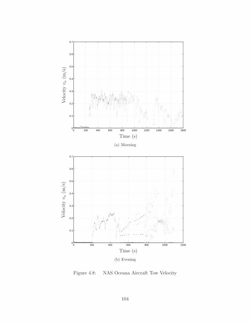
0 200 400 600 800 1000 1200 1400 1600 18000

0.1

0.2

0.3

0.4

0.5

0.6

0.7

Time (s)

Vel

oci

tyv

a(m

/s)

(a) Morning

0 200 400 600 800 1000 12000

0.1

0.2

0.3

0.4

0.5

0.6

0.7

Time (s)

Vel

oci

tyv

a(m

/s)

(b) Evening

Figure 4.8: NAS Oceana Aircraft Tow Velocity

104

Table 4.6: NAS Oceana Personnel Distance Statistics

Time Type p1 (m) p2 (m) p3 (m) p4 (m) p5 (m)

Morning Max 27.0057 4.5079 8.2550 26.5641 16.9151Mean 7.3512 2.3953 4.2892 2.8061 7.2944

Evening Max 5.9548 3.7441 4.0742 7.9871 30.4477Mean 3.8124 1.8905 2.5317 2.3566 6.4603

While six personnel were equipped with receivers during both the morning and

evening tow procedures, one of the Leica recorders failed to record its measurements.

This recorder had been provided to the starboard wing safety for the morning pro-

cedure, so there are no measurements available for this position. This failure was

noticed following the morning procedure and the device was reconfigured in hopes

of providing functionality for the evening procedure. In anticipation of a repeated

failure, the malfunctioning recorder was provided to a trainee acting as a secondary

in the wing safety role. The reconfiguration was unsuccessful and no evening data

was recorded by the malfunctioning device either.

It is also useful to observe the position of personnel involved relative to the

aircraft. Many of the mishaps discussed in Chapter I involve personnel being injured

by contact with aircraft landing gear or standing in a jet exhaust area. Figures 4.10

through 4.16 show the relative position for each phase of the morning tow procedure.

During this procedure, there were three phases where no motion of the aircraft oc-

curred. Figure 4.10 shows the motions of personnel preparing the aircraft to be towed

while Figures 4.12 and 4.14 show periods where the Director was consulting with the

Supervisor on the best course to take. The relative positions for the evening tow

procedure are provided in Figures 4.17 through 4.20.

105

0 200 400 600 800 1000 1200 1400 1600 18000

20

40

0 200 400 600 800 1000 1200 1400 1600 18000

5

0 200 400 600 800 1000 1200 1400 1600 18000

5

10

0 200 400 600 800 1000 1200 1400 1600 18000

20

40

0 200 400 600 800 1000 1200 1400 1600 18000

10

20

Time (s)

p1

(m)

p2

(m)

p3

(m)

p4

(m)

p5

(m)

(a) Morning

0 200 400 600 800 1000 12000

5

10

0 200 400 600 800 1000 12000

2

4

0 200 400 600 800 1000 12000

5

0 200 400 600 800 1000 12000

5

10

0 200 400 600 800 1000 12000

20

40

Time (s)

p1

(m)

p2

(m)

p3

(m)

p4

(m)

p5

(m)

(b) Evening

Figure 4.9: NAS Oceana Personnel Distance

106

−25 −20 −15 −10 −5 0 5 10 15 20−15

−10

−5

0

5

10

15

20

25

30

Lateral Location (m)

Lon

gitu

din

alLoca

tion

(m)

p1

p2

p3

p4

Figure 4.10: Relative Personnel Position - Morning - Setup

−25 −20 −15 −10 −5 0 5 10 15 20−15

−10

−5

0

5

10

15

20

25

30

Lateral Location (m)

Lon

gitu

din

alLoca

tion

(m)

p1

p2

p3

p4

Figure 4.11: Relative Personnel Position - Morning - First Move

107

−25 −20 −15 −10 −5 0 5 10 15 20−15

−10

−5

0

5

10

15

20

25

30

Lateral Location (m)

Lon

gitu

din

alLoca

tion

(m)

p1

p2

p3

p4

Figure 4.12: Relative Personnel Position - Morning - Preparing to Reverse

−25 −20 −15 −10 −5 0 5 10 15 20−15

−10

−5

0

5

10

15

20

25

30

Lateral Location (m)

Lon

gitu

din

alLoca

tion

(m)

p1

p2

p3

p4

Figure 4.13: Relative Personnel Position - Morning - Reversing

108

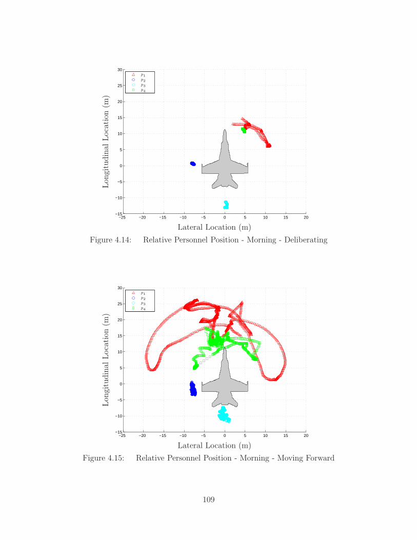
−25 −20 −15 −10 −5 0 5 10 15 20−15

−10

−5

0

5

10

15

20

25

30

Lateral Location (m)

Lon

gitu

din

alLoca

tion

(m)

p1

p2

p3

p4

Figure 4.14: Relative Personnel Position - Morning - Deliberating

−25 −20 −15 −10 −5 0 5 10 15 20−15

−10

−5

0

5

10

15

20

25

30

Lateral Location (m)

Lon

gitu

din

alLoca

tion

(m)

p1

p2

p3

p4

Figure 4.15: Relative Personnel Position - Morning - Moving Forward

109

−25 −20 −15 −10 −5 0 5 10 15 20−15

−10

−5

0

5

10

15

20

25

30

Lateral Location (m)

Lon

gitu

din

alLoca

tion

(m)

p1

p2

p3

p4

Figure 4.16: Relative Personnel Position - Morning - Reverse Parking

−25 −20 −15 −10 −5 0 5 10 15 20−15

−10

−5

0

5

10

15

20

25

30

Lateral Location (m)

Lon

gitu

din

alLoca

tion

(m)

p1

p2

p3

p4

p5

Figure 4.17: Relative Personnel Position - Evening - Setup

110

−25 −20 −15 −10 −5 0 5 10 15 20−15

−10

−5

0

5

10

15

20

25

30

Lateral Location (m)

Lon

gitu

din

alLoca

tion

(m)

p1

p2

p3

p4

p5

Figure 4.18: Relative Personnel Position - Evening - First Move

−25 −20 −15 −10 −5 0 5 10 15 20−15

−10

−5

0

5

10

15

20

25

30

Lateral Location (m)

Lon

gitu

din

alLoca

tion

(m)

p1

p2

p3

p4

p5

Figure 4.19: Relative Personnel Position - Evening - Deliberating

111

−25 −20 −15 −10 −5 0 5 10 15 20−15

−10

−5

0

5

10

15

20

25

30

Lateral Location (m)

Lon

gitu

din

alLoca

tion

(m)

p1

p2

p3

p4

p5

Figure 4.20: Relative Personnel Position - Evening - Second Move

−15 −10 −5 0 5 10 15−15

−10

−5

0

5

10

15

Lateral Location (m)

Lon

gitu

din

alLoca

tion

(m)

Figure 4.21: Relative Personnel Position - Wing and Tail Safeties

112

It is also possible to examine the relative position of both the Wing and Tail

Safeties throughout all the movement phases. The position of the Tractor Driver is

excluded as, during motion, they never leave the cart and the relative inaccuracy

present in the NovAtel measurements would cause too many errors in a similar anal-

ysis. The Director is excluded as only one individual fulfilling that role was measured

with a Leica recorder and as seen in Figures 4.10 through 4.20 their position can vary

greatly. The Supervisor is excluded as the position is not required onboard a U.S.

Navy aircraft carrier.

Figure 4.21 provides the relative location of the Wing and Tail Safeties through-

out all movement phases, both morning and evening. The data shows the aggregate

positions of five personnel, three as Wing Safety and two as Tail Safety. Using this

data it was straightforward to create bounding boxes as shown. With further study,

these bounding boxes could be treated as required positions for personnel towing an

aircraft. Bounding boxes for the Director and Tractor Driver could be created with

more data on their positions during an aircraft tow procedure. If a sailor leaves the

bounding box while the aircraft is in motion, the Director could be alerted.

4.2.5 Measurement Quality. The measurement quality statistics for both

the morning and evening phases are presented as Table 4.7. The mean DOP D is

fairly consistent across the devices during each phase. This is to be expected as

the satellite geometry shouldn’t have changed dramatically during each phase, but

may have between the phases. The high maximum DOP Dmax seen for some devices

corresponds to the personnel traveling underneath the aircraft’s wings.

4.2.6 Aircraft Wingfold. Following the conclusion of the evening tow proce-

dure, the personnel involved manually folded the wings of the aircraft. The wingspan

calculated from the recorder positions during this period are presented in Figure 4.22.

It is difficult, due to the noise in this data, to pick out the exact moment when the

wingfold procedure started. While it is possible to get a better approximation of the

113

Table 4.7: NAS Oceana Measurement Quality Statistics

Device Time Dmin Dmax D σD kmin kmax k σk

Left Morning 1.72 2.90 2.33 0.37 6 7 6.54 0.50Right Morning 1.72 2.90 2.35 0.37 6 7 6.52 0.50p1 Morning 1.77 7.28 2.45 0.54 4 7 6.48 0.56p2 Morning 1.43 2.90 2.22 0.32 6 8 6.74 0.45p3 Morning 1.30 8.06 2.45 0.78 4 8 6.49 0.57p4 Morning 1.77 10.95 2.79 0.92 4 7 6.44 0.60p5 Morning 1.77 7.17 2.86 0.66 6 7 6.51 0.50Left Evening 1.78 6.07 3.64 1.46 5 8 6.47 0.79Right Evening 1.47 3.81 2.81 0.93 5 8 6.24 0.95p1 Evening 1.46 13.08 2.95 1.61 4 9 6.24 1.29p2 Evening 1.62 9.82 3.02 1.44 4 9 6.47 1.05p3 Evening 1.46 10.98 3.03 1.38 4 9 6.53 1.09p4 Evening 1.40 9.69 3.55 1.51 4 9 6.31 1.02p5 Evening 1.40 9.98 3.93 1.78 4 9 6.04 0.96

Table 4.8: Wingfold Measurement Quality Statistics

Location Dmin Dmax D σD kmin kmin k σk

Left 4.11 11.99 5.46 1.27 4 6 5.37 0.56Right 3.70 13.32 4.42 0.89 4 7 5.22 0.70

time from personnel positions, this is of little use as the wingfolds this research is

concerned with are not performed manually.

Table 4.8 provides the measurement quality statistics for the wingfold proce-

dure. The mean DOP D is significantly higher during this procedure than during the

movement phases. This is likely due to the antenna direction as the wings are folded.

With the wings fully folded, the antennae pointed towards the center of the aircraft

rather than towards the sky.

4.2.7 Path Planning. In order for a persistent monitoring system to provide

early warnings of hazardous situations, it must be capable of predicting the path of

objects on the flight deck. If DIDO, the path planning software discussed in Sec-

114

1100 1150 1200 1250 1300 1350 1400 1450 15000

2

4

6

8

10

12

14

16

Time (s)

Win

gspan

b(m

)

Figure 4.22: Wingfold Wingspan Measurements

tion 2.7.3 on page 63, is provided a cost function J (x, u, t) which, when minimized,

simulates the objectives of the personnel involved in the towing procedure, then DIDO

should predict a path similar to the one taken. In the simulation, only forward motion

of the aircraft was allowed for simplification, however, this constraint could easily be

removed. The desired path, taken from the first portion of the evening phase, is shown

in Figure 4.23 and contains only forward motion. It is the first half of the movement

shown in Figure 4.7 but with the coordinate axes rotated so that the rows of parked

aircraft are aligned with the figure’s x-axis.

The procedures for towing aircraft are designed to minimize the risk to aircraft

and personnel. The decisions made by the personnel performing the tow procedure

should also be to minimize risk. From the path shown in Figure 4.23, it was observed

that straight paths are desired over long curves. This is likely due to greater risk of

collision with other aircraft or personnel during turns. The motion of the aircraft, two

articulated linkages behind the trailer, is more difficult for the Director and Tractor

Driver to predict while the system is turning. It is also more challenging for the Wing

and Tail Safeties to walk in a curve, rather than a straight line. So the tow tractor

115

60 80 100 120 140 160 180 200

−80

−60

−40

−20

0

20

40

x (m)

y(m

)

Figure 4.23: Path Planning: Desired Path

steering angle as a function of time α(t) should be minimized. A cost function which

simulates this desire for straight paths is given by

J (x, u, t) =

∫

|α(t)| dt. (4.1)

Other parameters could be used in the cost function as well. Minimizing ζ and φ

may provide even closer results. Using DIDO to find a path and minimizing this cost

provides the path shown in Figure 4.24. This path was generated by the MATLABr

scripts provided as Listings B.9 through B.13 on pages 160-177. The scripts used

for this problem were based on work by Hurni, et al. [20–22]. Over 30 minutes of

computation time was required to solve for the optimal path. While the paths do

not match exactly, this system can be used to warn personnel of potential mishaps

outside their field of view.

116

60 80 100 120 140 160 180 200

−80

−60

−40

−20

0

20

40

x (m)

y(m

)

Figure 4.24: Path Planning: Predicted Path

4.3 Summary

The ability of a radio-navigation based positioning system to measure the state

of the flight deck has been demonstrated using precision GPS recorders. The errors

observed in the measurements taken at NAS Oceana are consistent with expected GPS

errors. The position errors on the wingtips observed in the evening portion caused

measurement noise in the heading of the vehicle. Having observed the consistency

of personnel positions relative to the aircraft it is straightforward to envision how a

persistent monitoring system could recognize a potential mishap involving personnel.

The optimal path planning results, which closely match the actual path taken, could

enable a persistent monitoring system to recognize mishaps further ahead in time

than distance measurements alone.

117

V. Conclusions

The subject of this research was the feasibility of a persistent monitoring system

originally discussed in Section 1.3. Such a system would continually monitor

the position and orientation of all aircraft and support equipment, the position of

all personnel on the flight deck, and the state of critical flight deck systems such

as the up/down status of the jet blast deflectors. Such a system would provide this

information in a format easily understandable by decision makers, such as the Aircraft

Handling Officer, so that they can improve the safety and overall efficiency of flight

deck operations. The system should also autonomously notify personnel if they are

approaching a hazardous area or situation. The goal of such a system is a more

efficient flight deck which can

1. reduce the occurrence of flight deck mishaps and

2. provide accurate recordings of flight deck operations for analysis.

This chapter presents an overview of the research performed, how the knowledge

gained can be applied to the development of a persistent monitoring system, and

recommendations for future work in this area.

5.1 Overview

Chapter I provided a detailed analysis of the aviation mishap records provided

by the Naval Safety Center. This study showed that Interest Mishaps, those which are

potentially preventable by a persistent monitoring system, account for $92,486,469, or

5.55% of the cost of all recorded mishaps in the data provided. These Interest Mishaps

were categorized by cause and four successive levels of monitoring were proposed to

help mitigate their occurrence.

Prior research towards improving flight deck operations was explored in Chap-

ter II as well as related topics such as GPS, pseudolite positioning, and Blue Force

Tracking. Algorithms necessary to implement a persistent monitoring system were dis-

cussed including position and orientation determination as well as the nearest neighbor

118

problem. Multiple path planning methods were presented with the goal of predicting

the trajectory of a towed or taxiing aircraft.

The data collected for this research, discussed in Chapter III, involved mea-

suring the position and orientation of a towed aircraft as well as the position of the

personnel required for the procedure. Preliminary tests were conducted at AFIT to

ensure the proper operation of the GPS recorders and their ability to provide precision

measurements.

An analysis of the data collected, presented in Chapter IV, demonstrated the

ability of precision GPS recorders to measure the position and orientation of an air-

craft, both stationary and in motion, as well as the positions of personnel around it.

Significant error was observed in the evening tests, most likely caused by multipath.

The path planning software DIDO was used to find an optimal trajectory for the

towed aircraft system based upon the measured data.

From the results of this research, some overall conclusions can be made about

the feasibility of a persistent monitoring system:

1. Due to a number of factors, such as the high multipath error observed, the

high cost of dual frequency GPS receivers, the need for indoor functionality,

and the risks involved in relying on satellite transmissions, the measurement

system should not exclusively rely on GPS for the highly accurate measurements

required.

2. Substantial computing power is required to predict the path of a towed aircraft

and process state information from potentially hundreds of positioning devices.

The ability to closely match the actual path could significantly improve the

system’s ability to recognize potential mishaps.

5.2 Preventing Mishaps

With the knowledge and experience gained from the tests at NAS Oceana de-

scribed in Chapter III, it is possible to discuss how a persistent monitoring system

119

Barricade Stanchion

(a) Precise Measurement: The barricade stan-chion will impact the aircraft when raised.

Barricade Stanchion

(b) Imprecise Measurement: It is unknown ifthe barricade stanchion will impact the aircraftwhen raised.

Figure 5.1: Recognizing Spotting Mishaps

could be designed in order to prevent mishaps. Recalling the primary mishap classifi-

cations of Section 1.2.2, this section provides an example for each classification. Each

example is taken from the narratives of Table 1.4 on page 12.

5.2.1 Spotting Mishaps. An extremely common spotting mishap is a parked

aircraft being struck by a Jet Blast Deflector (JBD) or Barricade Stanchion. Fig-

ure 5.1 illustrates an aircraft parked such that the raising of a Barricade Stanchion

will impact the aircraft. A Level One system, one which measures aircraft position

and orientation, could potentially prevent such a mishap if the measurements are

sufficiently accurate.

A distance measurement between the aircraft and the barricade stanchion could

be used to recognize a potential mishap. If the distance between an aircraft’s center

and the barricade stanchion is below a certain threshold, then a nearest neighbor

search should be conducted to determine if any point on the aircraft is near zero

distance, in two-dimensions, from any point on the stanchion. If this is true, then a

persistent monitoring system could be set to handle the situation in different ways.

120

Having determined there is potential for a spotting mishap, the system could

warn the Taxi or Tow Director that the aircraft is parked in an undesirable location.

Alternately, the system could warn Flight Deck Control that the aircraft was parked

in a hazardous location, leaving it to the Handling Officer to determine whether it

should be moved. If the decision is made to park the aircraft in a potentially hazardous

position, for whatever reason, then the system could alert Flight Deck Control of this

hazard again if the Barricade Stanchions are set to be raised.

Considering the prevention of this type of mishap also allows an analysis of the

level of accuracy required for both position and orientation measurements. Figure 5.1

shows the effect of just 5 of heading angle measurement error. With this error a

monitoring system could not determine whether the stanchion would collide with the

aircraft.

The results of the heading calculations, presented in Figure 4.6 on page 101,

demonstrate the ability of precision GPS to provide accurate and low-noise headings.

Any radio navigation system with centimeter-level accuracy should be able to provide

similar results.

5.2.2 Towing Mishaps. Potential towing mishaps, such as a collision with a

parked aircraft in the hangar bay, could be recognized by a Level One system. A path

planning system, such as one that uses DIDO, discussed in Section 2.7.3 on page 63,

could continuously compute a reasonably close prediction of the path of the towed

aircraft system. If a Level Two system is implemented, it could monitor both aircraft

and support equipment.

Many towing mishaps listed in Appendix A involve a towed aircraft being parked

in close proximity to a stationary aircraft. Figure 1.16 on page 32 provides a visual-

ization of this close proximity. In this case, the persistent monitoring system could

continuously calculate the nearest neighbor distance to surrounding aircraft, equip-

ment, and personnel. If this distance is less than a pre-determined threshold, the

system could alert all personnel involved to the risk of collision.

121

Recognizing towing mishaps will be dependent upon the position measurement

accuracy of the system. As increased multipath errors were seen in the measurements

during the evening phase of the tests at NAS Oceana, described in Sections 4.2.1

and 4.2.2, this type of mishap may also dictate the requirements for maximum allow-

able multipath error. Figure 4.7 on page 103 shows that GPS can accurately measure

the location of the aircraft while Figure 4.9 on page 106 and Figure 4.21 on page 112

demonstrate the ability of GPS measurements to be utilized for personnel position

and nearest neighbor determination.

5.2.3 Taxiing Mishaps. A Level One system, measuring the position and

orientation of all aircraft on the flight deck, should be able to recognize a poten-

tial taxiing mishap. Typically, this type of mishap involves a collision between two

aircraft. While it could be possible to warn of such a potential mishap simply by

calculating the distance between the aircraft and their relative velocity, the use of

a path planning system, such as one that uses DIDO, discussed in Section 2.7.3 on

page 63, could significantly increase the time that personnel would be given to react

to the warning and reduce the occurrence of false warnings.

If a potential mishap is detected, the pilot of one aircraft could be directed to

stop while the other moves beyond the collision event horizon. In the case of a path

becoming obstructed, the Taxi Director and pilot could be provided with a new path

to follow.

5.2.4 Exhaust Mishaps. With the heading rate and personnel position mea-

surements from Sections 4.2.2 and 4.2.4 it is possible for a Level Three system to

recognize a potential exhaust mishap. In a typical scenario, the system could watch

for a taxiing aircraft performing a turn on deck with a sailor standing still in a location

the exhaust will pass through. Such a scenario is depicted in Figure 5.2.

To prevent injury or damage from resulting from this type of mishap, the sys-

tem could utilize not only the position and orientation measurements, but a desired

122

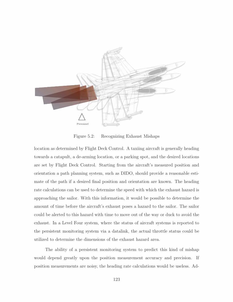
Personnel

Figure 5.2: Recognizing Exhaust Mishaps

location as determined by Flight Deck Control. A taxiing aircraft is generally heading

towards a catapult, a de-arming location, or a parking spot, and the desired locations

are set by Flight Deck Control. Starting from the aircraft’s measured position and

orientation a path planning system, such as DIDO, should provide a reasonable esti-

mate of the path if a desired final position and orientation are known. The heading

rate calculations can be used to determine the speed with which the exhaust hazard is

approaching the sailor. With this information, it would be possible to determine the

amount of time before the aircraft’s exhaust poses a hazard to the sailor. The sailor

could be alerted to this hazard with time to move out of the way or duck to avoid the

exhaust. In a Level Four system, where the status of aircraft systems is reported to

the persistent monitoring system via a datalink, the actual throttle status could be

utilized to determine the dimensions of the exhaust hazard area.

The ability of a persistent monitoring system to predict this kind of mishap

would depend greatly upon the position measurement accuracy and precision. If

position measurements are noisy, the heading rate calculations would be useless. Ad-

123

ditionally, the rapid pace of events on the flight deck could require the system to have

a particular measurement update rate to be fully effective.

5.2.5 Contact Mishaps. The contact mishap presented in Table 1.4 on

page 12 describes a Plane Handler, identified by the color of jersey worn, being run

over by the main mount of an aircraft. If a Level Three persistent monitoring system

is implemented it could issue warnings of such a situation. One potential prevention

method is to use the personnel bounding boxes shown in Figure 4.21 on page 112.

These bounding boxes are areas surrounding the aircraft where the personnel involved

are expected to remain throughout the procedure. The system could inform the

Director, Tractor Driver, and Plane Captain when all personnel are positioned within

the bounding boxes, and only then would they start moving the aircraft. If the pilot

is operating the aircraft, then the pilot could be given permission to move once all

personnel are positioned within their respective bounding boxes.

Preventing this type of mishap imposes requirements on the accuracy of both

aircraft and personnel position measurements. As personnel often travel underneath

the wing or fuselage of an aircraft during flight deck operations, it also presents

requirements for signal re-acquisition time for radio measurements or drift rate for

inertial measurements.

5.2.6 Engine Mishaps. As previously discussed, it is easy for a sailor to

walk directly into a turning propeller. With a Level Three system monitoring the

movements of personnel, the distance between a person and the propellor could be

measured and a warning issued if the distance is below a certain threshold. It would

also be possible to create a hazard zone directly in front of the propeller. If a person

enters the zone then the system would alert them to leave it immediately. Figure 5.3

illustrates notional hazard zones around the propellers of an E-2C Hawkeye.

The propeller hazard zones only exist when the propellers are turning. Mainte-

nance must be performed on the propellers, so the persistent monitoring system must

124

Personnel

Figure 5.3: Recognizing Engine Mishaps

somehow be aware of this status. An aircraft scheduled for a flight within a speci-

fied time, for instance, could automatically be checked for engine hazard violations.

Alternately, a supervisor on the flight deck could be required to inform Flight Deck

Control to disable the engine hazard violation warnings for maintenance purposes. If

a Level Four system is in place, then the engine status reported by the aircraft could

be utilized to determine hazard zone status.

5.2.7 Wingfold Mishaps. One method to potentially prevent wingfold

mishaps is a Level Four system, where the aircraft have been modified to report

their wingfold switch status to the persistent monitoring system. If the measured

position and orientation of the aircraft would force its unfolding wings to impact an-

other object, then the system would not allow the wings to unfold. This modification

could be prohibitively expensive, but future aircraft could have it included earlier in

the acquisition process at a reduced cost.

125

Another method to detect a potential wingfold mishap is to measure the distance

between wingtip mounted receivers as part of a Level One system. The rate at which

the wings were folded at NAS Oceana, presented in Section 4.2.6, was slow because the

fold was performed manually. When an FA-18C is powered, the wingfold process is

significantly faster. The magnitude of the wingspan measurement slope in Figure 4.22

on page 115 would be greater for a powered wingfold, and therefore easier to detect.

A persistent monitoring system’s performance specifications such as accuracy

and update rate will greatly affect its ability to recognize this type of mishap. Using

wingtip mounted receivers to detect the wingfold motion may also impose constraints

on the physical design of the receiver. Significant multipath was observed when the

wings were folded and the antennae were pointed towards the aircraft.

5.2.8 Non-aviation Mishaps. A non-aviation mishap, such as an aircraft

being struck by a forklift during an underway replenishment, is very similar to a

towing mishap. The same processes to recognize a potential mishap, path prediction

and distance calculation, should be applicable.

The challenge inherent to non-aviation mishaps is that they don’t exclusively

involve aviation assets or personnel. The forklifts and pallet jacks used by the supply

department would need to be monitored, and the personnel operating them would

have to be trained to respond to hazard warnings. Attempting to prevent this type

of mishap leads to considerations on the pervasiveness and simplicity of a persistent

monitoring system, as non-aviation personnel would only occasionally be required to

use it.

5.3 Measurement System Implementation

This section discusses the requirements for implementing methods to measure

the position and orientation of objects on the flight deck based upon the research

described in Chapter III. The equipment necessary to measure position and commu-

nicate hazard warnings is discussed.

126

5.3.1 Position Measurement. As discussed in Section 2.1.2 on page 36, the

Navy currently plans to use video analysis to measure the position and orientation of

each aircraft on the flight deck, although with less accuracy than the measurements

made in this research using GPS. To reduce the occurrence of flight deck mishaps,

one of the major goals of a persistent monitoring system, it is vital to not only

have accurate measurements of aircraft position and orientation but to measure the

position and orientation of support equipment as well as the position of personnel.

It may be possible to use additional cameras to measure these positions, but there

are numerous challenges. One challenge is identifying, via video recordings, a person

who may be standing up straight, crawling under an aircraft, or lying injured on

the deck. If this can be achieved, it is likely to require extensive computational

power. Radio navigation provides a simpler alternative and, as shown in Chapter IV,

the accuracy is significantly better than that expected of the planned video analysis

system. This section will focus on the methods of implementing a radio navigation

system to measure the location of aircraft, equipment, and personnel on the flight

deck and hangar bay.

5.3.1.1 Measurement Source. This research focused on using GPS

for position measurements. As discussed in Section 5.1, the exclusive use of GPS

is not desirable for a persistent monitoring system. The functionality of a system

reliant on GPS is at risk of degradation from multiple sources: satellite constellation

issues, atmospheric disturbance, as well as jamming or spoofing by an opposing force.

Furthermore, it is desired for this system to measure locations both on the flight deck

and the hangar bay. Given that the hangar bay is essentially one large Faraday cage,

and external radio transmissions cannot be received inside, it is impossible to use

GPS inside of it.

To achieve centimeter-level accuracy it is required to use a dual frequency GPS

receiver. Dual frequency antennae are expensive (each of the antennae used in this

research cost approximately $1,000), and a dual frequency receiver must either have

127

the classified decryption key for P(Y) code or, like the receivers used in this research,

advanced algorithms to utilize the L2 signal without decrypting P(Y), potentially

costing thousands of dollars per receiver. These costs are currently decreasing and

could potentially be further reduced given the mass production required to equip the

fleet.

Pseudolite positioning provides a promising alternative. With multiple trans-

mitters mounted on the flight deck and in the hangar bay the persistent monitoring

system should have observability of both areas. Pseudolites also provide the ability

to select the frequency and chipping rate of the transmission. With a higher chipping

rate or frequency transmission than GPS, highly accurate measurements could be

made using either code or carrier phase solutions, even on a single frequency. The

system would be organic to the ship enabling these parameters to be reconfigured

as the mission requires as well as eliminating the dependency on satellites. With

sufficient pseudolite transmitters around the perimeter of the flight deck, it could be

possible to avoid most scenarios where a receiver would be prevented from receiving

a signal due to another object’s obstruction.

Both GPS and pseudolite measurements are susceptible to multipath errors, as

observed in the wingspan and heading measurements of Chapter IV. This error will

likely be amplified onboard an aircraft carrier due to the large metal deck, metal su-

perstructure, and prevalence of other aircraft. To mitigate this, it may be necessary to

integrate inertial measurements with the code or carrier phase measurements through

a Kalman filter.

While this research has addressed the measurement accuracy needed for mishap

recognition, the measurement integrity of the system is critical to the proper operation

of a persistent monitoring system. Since the system is intended to enhance the safety

of personnel, it is vital that it be aware of any significant errors in the measurements.

5.3.1.2 Measurement Device. Position measurements are to be made

for three different objects: aircraft, support equipment, and personnel. If orientation

128

measurements are also desired, then the object would require two devices (or at least

two antennae). A common core device could be designed with additional compo-

nents specific to each object. The core device needs to make position measurements

and communicate these to a central computer onboard the ship wirelessly and in

near real-time. It would be possible for the core device to simply make pseudorange

measurements and transmit them via a packetized network protocol (such as IEEE

802.11) which would allow for the use of public/private key authentication to prevent

spoofing and allow identification. A centralized computer could then apply any error

corrections and calculate the actual relative flight deck positions and velocities. The

measurement device used must not add significant complication to flight deck oper-

ations. Battery management is likely to be a major user concern unless addressed

early in the design phase.

Simplifications can be included in the design of the measurement devices be-

cause they will operate primarily onboard the aircraft carrier. When a device can

communicate with the central onboard computer it needs only transmit the range in-

formation: no position computations need to be performed in the device. Offloading

computations would reduce the device’s processing power requirement and power con-

sumption. This centralization will also allow updates to the measurement algorithm,

including error corrections, to be applied centrally.

For aircraft position and orientation, the Navy must decide whether it is more

effective to modify the aircraft and install permanent receivers or to temporarily

mount them while the aircraft is on deck, similar to the method described in Sec-

tion 3.2.1 on page 77. In either case, it is vital that they are capable of transmitting

measurements whether the aircraft is powered or not. Support equipment presents a

unique challenge, as there are dozens of different types. It may be advantageous to

measure position and orientation only for SE over a certain threshold size. Position

measurements may also be needed for smaller SE such as ordnance carts and aircraft

jacks.

129

To enhance the safety of personnel, their device would require the largest num-

ber of features. It must not only collect and transmit range measurements but be

capable of providing warnings to the person using it. The device should not hinder

the movements of personnel any more than current flight deck protective equipment

does. The ideal device would integrate into existing helmets and/or float coats. Aural

warnings could be provided through noise-cancelling headphones, which could even

enable the wearer to be steered away from a hazardous area. The Navy and Air Force

are currently investigating active noise cancelling technology for use in high-noise

aviation environments which could be adapted to support this capability [55].

5.3.2 Flight Deck Status. It would be necessary to measure the elements

of flight deck state presented in Table 1.8 on page 23. Many of these are already

measured but it would be necessary to tie all of the measurements to a centralized

system.

5.3.3 Obstacles to Implementation. The single greatest obstacle to physical

implementation would likely be training personnel to use it properly. If decision

makers are not familiar with its capabilities, they will not use it to the full extent. If

sailors are not aware of its limitations they may rely on it too much for their safety.

Shipboard frequency allocation is a significant obstacle which would need to

be resolved. With multiple frequencies needed for pseudolite and wireless packetized

data transmission, it is vital that the system not interfere with existing systems or

pose a risk to electromagnetically sensitive equipment, such as ordnance.

5.4 Monitoring System Implementation

With a computer capable of collecting the position and state measurements of

objects on the flight deck, it is essential that software be created to fully utilize this

information. Many of the methods and algorithms discussed to recognize mishaps,

such as path planning and nearest neighbor searching, are computationally inten-

130

sive, requiring a high-performance computing infrastructure. The monitoring system

will also need to be highly reliable and survivable, able to withstand malfunctioning

components and damage. The monitoring system must be able to clearly and effec-

tively communicate with personnel in a variety of ways such as accepting inputs for

flight schedules and maintenance requests, displaying the current status and projected

configuration, and alerting personnel concerned to potential hazards.

5.4.1 Computational Requirements. Modern computers are significantly

more advanced than when CADOCS, discussed in Section 2.1.1, was proposed. The

tasks CADOCS was to perform, such as storing flight schedules, displaying a map of

the flight deck, and recording aircraft fuel and maintenance information, pushed the

limits of computational capacity. For a modern computer, these tasks are trivial.

Providing the ability to recognize and potentially prevent mishaps for a large

number of aircraft, equipment, and personnel requires a significant amount of com-

puting power. The central computer must calculate positions and orientations from

the ranges reported by each measurement device, perform hundreds of nearest neigh-

bor searches, and update path predictions at a rate which enables these calculations

to be useful. The measurements data for this research was collected at 5 Hz, which

is a reasonable requirement for the onboard computer system. As discussed in Sec-

tion 2.6.1, the nearest neighbor calculation time is dependent upon the number of

points composing the model, so the system developers will have to trade model reso-

lution, calculation rate, and computational power.

The path planning algorithm is orders of magnitude more computationally in-

tensive than the other algorithms discussed. Using DIDO in MATLABr to calculate

the results presented in Section 4.2.7 required over 30 minutes on a computer with a

dual-core processor. Implementing this for a real-time operational system will require

rewriting an optimal solver in a lower-level language, such as C or C++, utilizing

multiple computers in a massive parallel system, or both. While this is the most com-

131

putationally intensive portion of the hazard recognition process, it has the potential

to provide the greatest benefit.

Another consideration that should be taken into account in the development of a

persistent monitoring system is the need for redundancy, reliability, and maintainabil-

ity. If the central computer ceases to function, for whatever reason, the entire system

would cease to function. Parallel computing provides a straightforward solution to

this problem. Multiple spaces, spread throughout the ship, could be utilized to house

the computers for this system. This has the added advantage of making the system

highly maintainable as a single faulty computer could be replaced without disabling

the system.

5.4.2 Human-Computer Interaction. No matter how well the system is

able to recognize and potentially prevent mishaps, it won’t be used if the personnel

concerned can’t fully interact with it. The input method for providing schedules,

requests, and orders must be intuitive. A user should be able to immediately recognize

and understand the information provided by a display. Warnings need to be effective

without hindering flight deck operations.

A touch-sensitive table computer, depicted in Figure 2.3 on page 36, seems to

be the perfect method for human-computer interaction within flight deck control.

Movement orders can be provided simply by touching, dragging, and rotating the

icon for an aircraft. Multiple users can even use the system simultaneously. Critical

information, such as fuel state, maintenance status, and next scheduled flight could

be accessed with the touch of a finger.

Maintenance personnel throughout the ship could be provided with flight deck

and hangar bay information through a web browser based system. This could allow

maintenance requests to be communicated effectively to flight deck control and aircraft

movement schedules to be accessed directly by the personnel directed to perform

maintenance. The web browser based interface would allow access without any special

software and updates to be applied only to a central computer.

132

5.4.3 Data Recording. Part of preventing mishaps is studying the exact

events that occurred. The monitoring system could record all of its information for

later access in the case of a mishap, much as an aircraft records data to the “black

box.” This data could be archived with organizations concerned, such as the Naval

Safety Center and Naval Air Systems Command, for thorough study to improve not

just safety, but the performance of flight deck operations.

In the event of a mishap, the ship or squadron would be able to review the

events in detail with the personnel involved. This provides an objective recording of

mistakes from which to learn. Simply reviewing the data collected could potentially

be of greater value than the real-time monitoring provided by the system.

5.5 Future Work

The persistent monitoring system proposed by this research is complex, and

no off-the-shelf product can provide its capabilities. Since the proposed system is

modular, with independent subsystems for measurement and monitoring, future work

in this area can explore each simultaneously.

The development of the measurement system requires more study of radio posi-

tioning in an environment similar to the flight deck. Further research into integrating

inertial and radio navigation measurements for multipath error mitigation should be

performed. The use of pseudolites, near ground level, to provide two-dimensional

positioning on a moving platform also requires significant research.

Further research in using path planning to match the movements of aircraft on

the flight deck is critical to the monitoring system. Determining the correct param-

eters to calculate the cost function could significantly improve the accuracy of the

predicted path. Other research should focus on the best methods of interacting with

personnel, and what functionality experienced personnel would find useful.

133

5.6 Final Thoughts

This research set out to determine the feasibility of utilizing a persistent mon-

itoring system to potentially prevent mishaps onboard a U.S. Navy aircraft carrier.

From the data collected it is clear that radio navigation can provide the accuracy to

collect the information necessary to recognize a hazardous situation. Actually im-

plementing a system to provide this functionality is a complex and challenging task.

Arguments have been provided that significant cost savings could be achieved by im-

plementing such a system. It is up to Naval leadership to determine if the operational

and safety benefits outweigh the costs.

134

Appendix A. Interest Mishaps

The records provided by the Naval Safety Center contained information on 3,228

mishaps. Those that were identified by the author as potentially preventable,

here labelled Interest Mishaps, are those in which a persistent monitoring system for

the flight deck could have provided some warning.

Many of the data elements provided, described in Table 1.1 on page 6, are

provided here. If multiple aircraft were involved in the mishap, only the first is listed

under Type/Model/Series. The Fatalities and Major Injuries columns were generated

by reading the narratives. A tally was made only when the narrative specifically

stated a sailor was injured or killed. The category column represents the mishap

classification as described in Section 1.2.2 on page 9.

Narratives are presented exactly as contained in the data provided by the Naval

Safety Center. Some commonly used abbreviations not previously explained which

may be unclear to readers without Naval experience are:

1. P/C or PC: Plane Captain

2. GSE: General Support Equipment

3. STBD: Starboard

4. MLG: Main Landing Gear

5. SQN: Squadron

6. ABH-2: Aviation Boatswain’s Mate (Handling) Second Class

7. CQ: Carrier Qualifications

8. LEF: Leading Edge Flap

135

Interest Mishaps.

Event

Serial

Fiscal

Year

Event Class Type Model

Series

Total Event

Cost ($)

Fatalities Major Injuries Narrative Category

31164 1980 A GROUND F004N 2,679,830 0 0 ACFT ROLLED OFF FLT DECK AND SANK WHILE SHIP

WAS PERFORMING PORT TURN.

Spotting

31266 1980 B GROUND F014A 34,000 0 1 CHOCK WALKER SUSTAINED MAJ INJURY WHEN FOOT

WAS RUN OVER BY TOWED ACFT

Contact

31656 1980 B GROUND E002B 34,000 0 1 P/C SUSTAINED MAJOR INJURIES WHEN HE WALKED

INTO ARC OF TURNING PROP.

Engine

31708 1980 B FLIGHT A007E 273,102 0 0 CHOCK CART AND CHOCKS BLOWN INTO TURNING

PROPS BY JET BLAST.

Exhaust

31720 1980 B FLIGHT A007E 151,789 0 0 A/C TAXIING ON CV STRUCK SECOND A/C AND 2 FLT

DK PERSONNEL CAUSING INJ

Taxi

31739 1980 B GROUND S003A 120,064 0 0 ACFT BACKED INTO PARKED ACFT WING BUTT DUR-

ING DECK RESPOT.

Towing

31740 1980 B GROUND S003A 128,636 0 0 ACFT BACKED INTO WING BUTT OF PARKED ACFT

DURING DECK RESPOT.

Towing

29567 1981 A FLIGHT S003A 106,937 1 0 ACFT JET ENG INGESTED MAINT TROUBLESHOOTER

DURING TURN-UP ON CV. FATAL

Engine

29757 1981 C GROUND F014A 22,760 0 0 ACFT SUSTAINED DAMAGE TO A/B SUPPORT DURING

DECK RESPOT.

Spotting

29763 1981 C FLTREL A007E 285 0 0 GSE OPERATOR INJURED WHEN BLOWN OFF POWER

CART BY JET BLAST.

Exhaust

30143 1981 A FLTREL A006E 151,000 0 1 JET BLAST STRUCK FINAL CHECKER ON FLT DECK

RESULTING IN MAJOR INJURIES

Exhaust

30222 1981 B FLIGHT HH046A 337,050 0 0 ACFT ROLLED ONTO SIDE AFTER STBD MLG BECAME

FOULED IN CV ELEV COMBING.

Towing

30345 1981 B FLIGHT TE002A 107,171 0 0 PROP STRUCK BY JBD PANEL AS ACFT TAXIIED INTO

POSITION FOR CAT LAUNCH

Taxi

30422 1981 A FLTREL A007E 37,000 1 0 LINE DIV DAY SUPER BLOWN OVER THE SIDE BY JET

BLAST. FATALLY INJURED.

Exhaust

31798 1981 A GROUND RF008G 500,000 0 0 AIRCRAFT UNDER TOW STRUCK WING OF PARKED

AIRCRAFT ON FLIGHT DECK.

Towing

31865 1981 A GROUND F014A 13,997,000 0 0 ACFT SPOTTING DOLLY LOST OVERBOARD DURING

ACFT SPOTTING OP AT SEA.

Spotting

31915 1981 A GROUND F014A 724,000 0 0 PARKED ACFT SUSTAINED ALPHA DAMAGE WHEN

STRUCK BY CLOSING HGR BAY DOOR

Spotting

Continued on next page

136

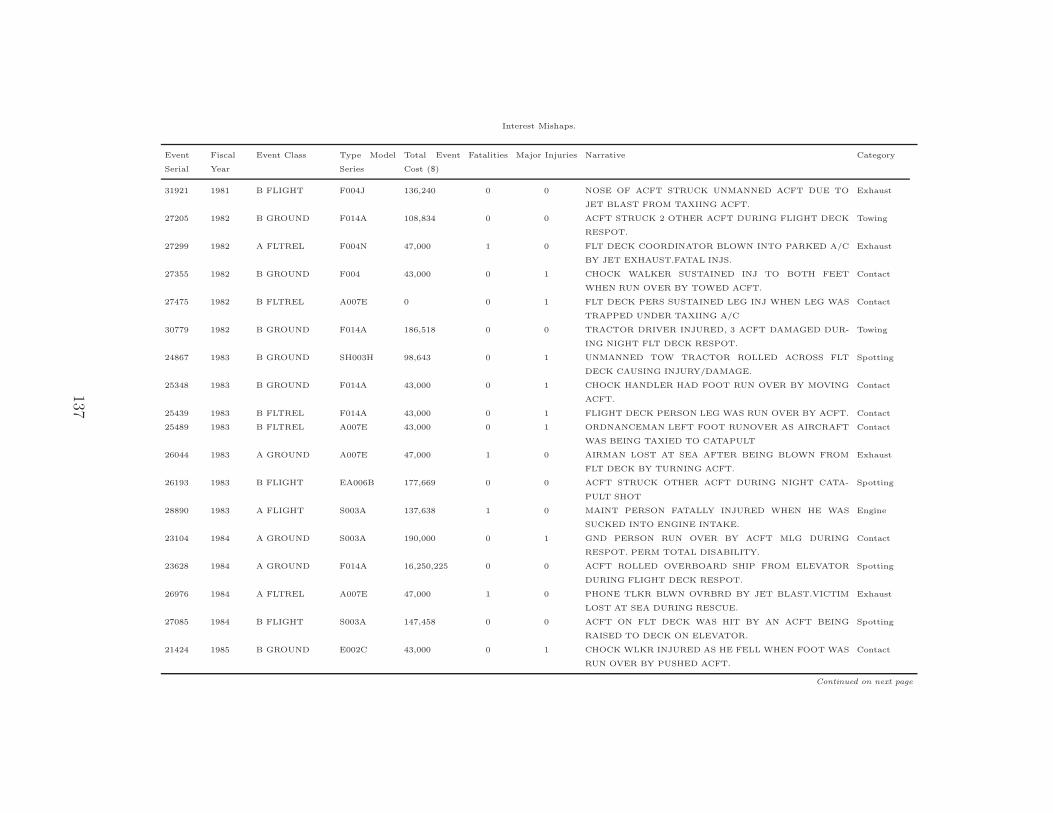
Interest Mishaps.

Event

Serial

Fiscal

Year

Event Class Type Model

Series

Total Event

Cost ($)

Fatalities Major Injuries Narrative Category

31921 1981 B FLIGHT F004J 136,240 0 0 NOSE OF ACFT STRUCK UNMANNED ACFT DUE TO

JET BLAST FROM TAXIING ACFT.

Exhaust

27205 1982 B GROUND F014A 108,834 0 0 ACFT STRUCK 2 OTHER ACFT DURING FLIGHT DECK

RESPOT.

Towing

27299 1982 A FLTREL F004N 47,000 1 0 FLT DECK COORDINATOR BLOWN INTO PARKED A/C

BY JET EXHAUST.FATAL INJS.

Exhaust

27355 1982 B GROUND F004 43,000 0 1 CHOCK WALKER SUSTAINED INJ TO BOTH FEET

WHEN RUN OVER BY TOWED ACFT.

Contact

27475 1982 B FLTREL A007E 0 0 1 FLT DECK PERS SUSTAINED LEG INJ WHEN LEG WAS

TRAPPED UNDER TAXIING A/C

Contact

30779 1982 B GROUND F014A 186,518 0 0 TRACTOR DRIVER INJURED, 3 ACFT DAMAGED DUR-

ING NIGHT FLT DECK RESPOT.

Towing

24867 1983 B GROUND SH003H 98,643 0 1 UNMANNED TOW TRACTOR ROLLED ACROSS FLT

DECK CAUSING INJURY/DAMAGE.

Spotting

25348 1983 B GROUND F014A 43,000 0 1 CHOCK HANDLER HAD FOOT RUN OVER BY MOVING

ACFT.

Contact

25439 1983 B FLTREL F014A 43,000 0 1 FLIGHT DECK PERSON LEG WAS RUN OVER BY ACFT. Contact

25489 1983 B FLTREL A007E 43,000 0 1 ORDNANCEMAN LEFT FOOT RUNOVER AS AIRCRAFT

WAS BEING TAXIED TO CATAPULT

Contact

26044 1983 A GROUND A007E 47,000 1 0 AIRMAN LOST AT SEA AFTER BEING BLOWN FROM

FLT DECK BY TURNING ACFT.

Exhaust

26193 1983 B FLIGHT EA006B 177,669 0 0 ACFT STRUCK OTHER ACFT DURING NIGHT CATA-

PULT SHOT

Spotting

28890 1983 A FLIGHT S003A 137,638 1 0 MAINT PERSON FATALLY INJURED WHEN HE WAS

SUCKED INTO ENGINE INTAKE.

Engine

23104 1984 A GROUND S003A 190,000 0 1 GND PERSON RUN OVER BY ACFT MLG DURING

RESPOT. PERM TOTAL DISABILITY.

Contact

23628 1984 A GROUND F014A 16,250,225 0 0 ACFT ROLLED OVERBOARD SHIP FROM ELEVATOR

DURING FLIGHT DECK RESPOT.

Spotting

26976 1984 A FLTREL A007E 47,000 1 0 PHONE TLKR BLWN OVRBRD BY JET BLAST.VICTIM

LOST AT SEA DURING RESCUE.

Exhaust

27085 1984 B FLIGHT S003A 147,458 0 0 ACFT ON FLT DECK WAS HIT BY AN ACFT BEING

RAISED TO DECK ON ELEVATOR.

Spotting

21424 1985 B GROUND E002C 43,000 0 1 CHOCK WLKR INJURED AS HE FELL WHEN FOOT WAS

RUN OVER BY PUSHED ACFT.

Contact

Continued on next page

137

Interest Mishaps.

Event

Serial

Fiscal

Year

Event Class Type Model

Series

Total Event

Cost ($)

Fatalities Major Injuries Narrative Category

24264 1985 B GROUND F014A 257,102 0 0 ACFT STRUCK PARKED ACFT DURING RESPOT EVO-

LUTION.

Taxi

24447 1985 A GROUND KA006D 47,000 1 0 GND PERSON RECEIVED FATAL INJ WHEN BLOWN

OVERBD DURING NIGHT LAUNCH.

Exhaust

17534 1986 A FLTREL A007E 47,000 1 0 FLT DECK PERS BLOWN OVERBOARD BY JET BLAST

DUR LAUNCH W/FATAL INJURY.

Exhaust

18846 1986 A FLIGHT S003A 209,954 1 0 ACFT HIT GROUND PERSON DURING NIGHT CATA-

PULT LAUNCH WITH FATAL INJURY.

Contact

18952 1986 B GROUND A006E 43,000 0 1 ACFT UNDER TOW ROLLED OVER ORDNANCEMAN’S L

LEG DURING DECK RESPOT.

Contact

19051 1986 C FLIGHT F018A 89,142 0 0 ACFT UNDER TOW RUNS OVER ACFT HANDLER’S LEG. Contact

22273 1986 B GROUND SH003H 129,932 0 0 PARKED ACFT SUSTAINED DAMAGE WHEN BARRI-

CADE STANCHION STRCK HORIZ STAB

Spotting

22622 1986 B GROUND F018A 43,000 0 1 CHOCK WALKER HAD FOOT RUN OVER BY ACFT DUR-

ING SPOTTING OPERATION.

Contact

14396 1987 B FLIGHT E002C 328,404 0 0 ACFT DAMAGE/PERS INJURIES RESULT FROM DECK

RAMP BLOWN BY JET EXHAUST

Exhaust

15008 1987 B FLTREL A007E 43,000 0 1 ACFT TAXIED OVER FINAL CHECKER’S LEGS. Contact

15258 1987 B GROUND KA003B 43,000 0 1 ACFT HANDLING CREWMAN’S LEG WAS RUN OVER

DURING ACFT RESPOT ON CV.

Contact

15881 1987 A GROUND F014A 553,839 0 0 ACFT HIT MULTIPLE ACFT WHILE BEING PUSHED TO

RESPOT POSITION.

Towing

19749 1987 A FLIGHT A007E 2,839,435 0 0 ACFT WENT OVER PORT SIDE OF SHIP DURING TAXI.

ACRW EJECTED.

Taxi

7671 1988 A GROUND A007E 2,877,000 1 0 DUR RESPOT SLID OFF FLT DECK WHILE UNDER TOW.

P/C MISSING.

Towing

8158 1988 A FLIGHT C002A 78,204 1 0 SQN PLANE CAPTAIN WALKED INTO ACFT PROP FOL-

LOWING NORMAL RECOVERY.

Engine

8368 1988 B FLIGHT F014A 105,761 0 0 INADVERTENT WINGSWEEP ON DECK. WING STRUCK

ANOTHER ACFT.

Wingfold

8739 1988 B FLTREL EA006B 45,700 0 1 MAIN MOUNT STRUCK SHUTTLE, TIRE EXPLODED IN-

JURING YELLOW SHIRT.

Misc

16200 1988 B GROUND A006E 43,000 0 1 ACFT RAN OVER PLANE CAPT TRAINEE’S LEG DUR-

ING NIGHT FLT DECK RESPOT.

Contact

16384 1988 A FLIGHT E002C 77,199 1 0 DURING PREP FOR LAUNCH, GROUND PERSON

WALKED INTO TURNING PROPELLER.

Engine

Continued on next page

138

Interest Mishaps.

Event

Serial

Fiscal

Year

Event Class Type Model

Series

Total Event

Cost ($)

Fatalities Major Injuries Narrative Category

16519 1988 B FLIGHT E002C 116,404 0 0 ACFT UNDER DIRECTOR CONTROL TAXIIED INTO

TURNING PROP. NO INJURIES.

Taxi, engine

1408 1989 B GROUND E002C 344,390 0 0 ACFT TAXIIED INTO TURNING PROP OF ANOTHER

ACFT.

Taxi, engine

5630 1990 A GROUND EA006B 1,310,570 0 0 ECM POD INADVERTENTLY FIRED DUE TO EXHAUST

EXPOSURE.

Exhaust

32216 1991 B GROUND F014B 320,962 0 0 TAXIING ACFT STRUCK TWO OTHER ACFT ON CAR-

RIER FLIGHT DECK.

Taxi

33679 1991 B GROUND S003B 294,597 0 0 PARKED ACFT SLID INTO CATWALK DURING SHIPS

TURN.

Spotting

40078 1991 C GROUND F018C 98,524 0 0 ACFT HORIZ STAB, DOORS WERE BURNT BY EXHAUST

OF ANOTHER ACFT

Exhaust

35370 1992 A GROUND F014A 500,000 0 1 BLUE SHIRT RUN OVER BY ACFT MAIN MOUNT. Contact

35480 1992 B GROUND EA006B 115,000 0 0 DUR ACFT TAXI JET BLAST BLEW ABH-2 FROM FLT

DECK TO LOWERED ELEVATOR.

Exhaust

37767 1993 B GROUND F014A 115,000 0 1 FLIGHT DECK PERSON PULLED INTO ACFT INTAKE. Engine

37867 1993 C GROUND SH060F 31,338 0 0 ACFT WING SPREAD INTO HELO ON HANGAR BAY. Wingfold

38669 1993 A GROUND A006E 270,000 0 1 MAINT PERS BLOWN OVERBD BY JET EXHAUST

WORKING ON FLT DECK.

Exhaust

38778 1993 C GROUND EA006B 57,809 0 0 CATAPULT 2 JBD STRUCK ACFT LEFT WING TIPE DUR-

ING ACFT TAXI.

Taxi

39865 1994 C GROUND A006E 13,048 0 1 ACFT TAXIED ONTO FINAL CHECKER’S ANKLE DUR-

ING ACFT SPOT ON CATAPULT.

Contact

40106 1994 C GROUND EA006B 63,166 0 0 PARKED AIRCRAFT STRUCK BY TOW TRACTOR ON

FLIGHT DECK.

Spotting

40139 1994 C GROUND F018C 50,438 0 0 DEPLOY OPS/UNDER FLT DECK DIR/NIGHT POST RE-

COVERY, ACFT HIT PARKD ACFT

Taxi

40155 1994 C GROUND F018C 15,828 0 0 PARKED ACFT WAS STRUCK BY ACFT UNDER TOW

DURING FLT DECK RESPOT.

Towing

40431 1994 C GROUND SH003H 155,979 0 0 DURING NIGHT FLT DECK RESPOT ACFT UNDER TOW

HIT HELO PARKED ON SPOT 5.

Towing

40688 1994 C GROUND F014D 50,336 0 0 ACFT UNDER TOW IN HANGAR DECK BAY COLLIDED

WITH PARKED ACFT.

Towing

40775 1994 GRND HZ: GEN-

ERAL

A006E 0 0 0 ACFT PORT OUTBOARD WING TIP WAS HIT BY JET

BLAST DEFLECTOR.

Unknown

Continued on next page

139

Interest Mishaps.

Event

Serial

Fiscal

Year

Event Class Type Model

Series

Total Event

Cost ($)

Fatalities Major Injuries Narrative Category

40832 1994 GRND HZ: GEN-

ERAL

E002C+ 0 0 0 HYD JENNY ROLLED INTO HAWKEYE DAMAGING

FUSELAGE.

Spotting

40910 1994 C GROUND F018C 15,852 0 0 ACFT UNDER TOW AND CONTROL OF FLT DECK DI-

RECTORS HIT ANOTHER ACFT.

Towing

41057 1994 GRND HZ: GEN-

ERAL

F018C 0 0 0 ACFT WITH CAPTIVE TRNG ORD CONTACTED GSE ON

CV FLT DECK ON CQ OPS

Unknown

40888 1995 B GROUND F018C 115,000 0 1 ACFT UNDER TOW RAN OVER AIRMAN ON FLIGHT

DECK.

Contact

40990 1995 B GROUND EA006B 115,000 0 1 ORDNANCEMAN SUFFERED CRUSHED FOOT FROM

TAXIING ACFT ON FLIGHT DECK.

Contact

41428 1995 B GROUND F014A 456,386 0 0 ACFT BLOWN INTO CATWALK BEHIND CAT 4; AIR-

CREW EJECTED SAFELY.

Exhaust

41451 1995 C GROUND C002A 16,569 0 1 ENG NAC PANELS LOST OVRBD & MAINT MAN BLOWN

DOWN BY JET BLAST ON DECK.

Exhaust

41501 1995 C GROUND F018C 40,000 0 0 ACFT RADOME DAMAGED AFTER COLLISION WITH

ANOTHER ACFT ON FLT DECK.

Unknown

42144 1995 C GROUND EA006B 0 0 1 DURING NIGHT FRS CQ AIRCRAFT TAXIED OVER AIR-

MAN’S FOOT.

Contact

42699 1995 C GROUND F018C 13,177 0 0 ACFT RADOME STRUCK RIGHT HORIZ STAB OF AN-

OTHER ACFT DURING TAXI.

Taxi

42963 1996 C GROUND ES003A 31,904 0 0 GSE HIT ACFT PORT SIDE CAUSING DAMAGE TO ENG

INLET COWL & ARS RAT

Spotting

43036 1996 C GROUND S003B 21,300 0 0 ACFT RUDDER HIT CVN ISLAND, PLAT PLATFORM,

WHILE BEING TAXIED ON DECK.

Taxi

43137 1996 FLT HZ: GEN-

ERAL

EA006B 0 0 0 FLT DECK HATCH ON UPPER STAGE WEAPONS ELEV

2 OPENED DAMAGING ALQ-99.

Spotting

43424 1996 C GROUND F018C 94,029 0 0 CAT 2 JBD WAS RAISED INTO LEFT WING OF ACFT IN

DEARMING AREA.

Spotting

43473 1996 C GROUND F018A 48,966 0 0 DURING NIGHT FLIGHT DECK OPERATIONS, ACFT

TAXIED INTO PARKED ACFT.

Taxi

43581 1996 C GROUND F018C 26,930 0 0 AIRCRAFT UNDER TOW ON FLIGHT DECK IMPACTED

LSO PLATFORM WINDSCREEN.

Towing

43641 1996 C GROUND F018C 29,417 0 0 FORKLIFT OPERATOR STRUCK HORIZ STAB OF

PARKED ACFT DURING VERTREP.

Misc

43970 1996 B GROUND F018C 245,252 0 0 CRANE OPERATOR INADVERTENTLY LIFTED ACFT

WHILE STILL CHAINED DOWN.

Misc

Continued on next page

140

Interest Mishaps.

Event

Serial

Fiscal

Year

Event Class Type Model

Series

Total Event

Cost ($)

Fatalities Major Injuries Narrative Category

44056 1996 C GROUND EA006B 1,875 0 0 TAILHOOK LOWERED ONTO FUEL HANDLER MAN-

NING REFUELING STA IN CATWALK.

Contact

44099 1996 GRND HZ: GEN-

ERAL

EA006B 0 0 0 TOW TRACTOR COLLIDED WITHALQ-99 POD

RADOME.

Towing

44447 1996 GRND HZ: GEN-

ERAL

S003B 0 0 0 ACFT CARRIER JET BLAST DEFECTOR RAISED INTO

TAXIING ACFT.

Taxi

44458 1996 GRND HZ: GEN-

ERAL

E002C+ 0 0 0 UHF SATCOM ANTENNA DAMAGED WHILE TOWING

ACFT IN HANGAR BAY

Towing

44473 1996 A GROUND F014A 500,000 0 1 GROUND HANDLER RUN OVER BY ACFT UNDER TOW.

PERM TOTAL DISABILITY.

Contact

45407 1996 GRND HZ: GEN-

ERAL

EA006B 0 0 0 ACFT TAXIED INTO NOSE RADOME OF ANOTHER

ACFT. FOD INGESTED BY STBD ENG

Taxi

45035 1997 GRND HZ: GEN-

ERAL

F018C 0 0 0 WINGS WERE INADVERTENTLY SPREAD DURING

START UP, DAMAGING CATM9 MISSIL

Wingfold

45403 1997 GRND HZ: GEN-

ERAL

F018C 0 0 0 WINGS WERE INADVERTENTLY SPREAD DURING FLT

DECK MAINT, DAMAGING AIM9.

Wingfold

45554 1997 GRND HZ: GEN-

ERAL

S003B 0 0 0 ACFT STRUCK TOW TRACTOR DURING RESPOT ON

SLIPPERY DECK & HIGH SEAS.

Towing

45584 1997 C GROUND S003B 58,504 0 0 TOW TRACTOR STRUCK ACFT DURING FLIGHT DECK

RESPOT.

Towing

45629 1997 C GROUND F018 25,940 0 0 DURING TAXI, ACFT HIT PARKED ACFT ON FLIGHT

DECK.

Taxi

45766 1997 GRND HZ: GEN-

ERAL

E002C 0 0 0 MAINT PERSONNEL BLOW INTO FANTAIL SAFETY NET

DURING ACFT MAINT TURN.

Exhaust

46014 1997 GRND HZ: GEN-

ERAL

E002C 0 0 1 FINAL CHECKER TRAINEE BLOWN OVER JBD DURING

AIRCRAFT RUN-UP ON CAT.

Exhaust

46047 1997 C GROUND F014A 13,110 0 0 DURING HANGAR BAY RESPOT, ACFT COLLIDED

WITH ADJACENT CHANIED ACFT.

Towing

46119 1997 C GROUND F018A 44,528 0 0 ACFT SUSTAINED DAMAGE TO RADOME DURING

HANGAR DECK RESPOT.

Towing

46203 1997 GRND HZ: GEN-

ERAL

F018C 0 0 0 ACFT AT HIGH POWER DURING TAXI BLEW PRE-

FLIGHTING AIRCREW INTO CATWALK

Exhaust

46269 1997 C GROUND F018C 54,417 0 0 ACFT SUSTAINED DMG TO LEADING EDGE FLAP

WHEN JBD WAS RAISED INTO IT.

Spotting

46536 1997 C GROUND F018C 199,522 0 0 ACFT RADOME STRUCK BY WING BUTT OF TAXIING

ACFT ON FLIGHT DECK.

Taxi

Continued on next page

141

Interest Mishaps.

Event

Serial

Fiscal

Year

Event Class Type Model

Series

Total Event

Cost ($)

Fatalities Major Injuries Narrative Category

46704 1997 GRND HZ: GEN-

ERAL

S003B 0 0 0 TOW TRACTOR HIT AERIAL REFUELING STORE ON

FLT DECK.

Towing

46852 1997 C GROUND E002C+ 61,073 0 0 ACFT 01 TAXIED INTO TURNING ACFT 02 PROP DAM-

AGING BOTH ACFT.

Taxi, engine

47263 1998 C GROUND F018C 25,940 0 0 ACFT UNDER TOW STRUCK LSO PLATFORM DURING

NIGHT FLIGHT DECK RESPOT.

Towing

47376 1998 C GROUND EA006B 18,965 0 0 TOW TRACTOR COLLIDED WITH ACFT AND INJURED

TROUBLESHOOTER

Towing

47618 1998 C GROUND F018C 66,670 0 0 AIRCRAFT TOWED INTO PARKED AIRCRAFT. Towing

47643 1998 GRND HZ: GEN-

ERAL

E002C+ 0 0 1 PLANE CAPTAIN STRUCK BY TURNING PROPELLER. Engine

47673 1998 GRND HZ: GEN-

ERAL

F018C 0 0 0 ACFT RADOME IMPACTED BY AILERON OF SECOND

ACFT WHICH WAS TAXIING ON DK

Taxi

47772 1998 GRND HZ: GEN-

ERAL

EA006B 0 0 0 CAT CREW RETRACTED SHUTTLE INTO ACFT PORT

MAIN TIRE;INADEQ COORDINATIO

Spotting

47870 1998 C GROUND F018C 45,676 0 0 STARBOARD HORIZONTAL STABILIZER DMGD WHEN

STRUCK BY FORKLIFT.

Misc

47904 1998 GRND HZ: GEN-

ERAL

F018C 0 0 0 RIGHT HORIZONTAL STAB STRUCK ANOTHER ACFTS

LEF DUR FLT CNTRL CAS CKS.

Spotting

48805 1999 C FLIGHT S003B 22,406 0 0 FLIGHT DECK PERSONNEL DROVE TOW TRACTOR

INTO BUDDY STORE OF AIRCRAFT.

Towing

48838 1999 C GROUND E002C 33,739 0 0 WING TIP OF TAXIING ACFT STRUCK PROP OF

PARKED ACFT ON FLIGHT DECK.

Taxi, engine

49159 1999 C GROUND C002A 23,256 0 0 TAILSKID HIT SCUPPER, BREAKING ACTUATOR FIT-

TING.

Unknown

49612 1999 C GROUND F018C 16,241 0 0 DUR LOW PWR TURN, INADVERTENT WINGSWEEP

CAUSED STBD WING TO HIT AILERO

Wingfold

49753 1999 GRND HZ: GEN-

ERAL

C002A 0 0 0 STBD WING TIP HIT TOP OF COMBAT HATCH DURING

WINGSPREAD EVOLUTION.

Wingfold

49776 1999 C GROUND HH060H 22,900 0 0 TAIL ROTOR BLADE OF PARKED AIRCRAFT DAMAGED

BY CRASH CRANE.

Misc

49853 1999 GRND HZ: GEN-

ERAL

F018C 0 0 0 MISPOSITIONED WINGFOLD HANDLE RESULTED IN IN-

ADVERT WINGSPREAD ON START

Wingfold

49899 1999 C GROUND F014D 177,287 0 0 AIRCRAFT STRUCK BY JET BLAST DEFLECTOR

WHILE TAXIING TO CATAPULT.

Taxi

Continued on next page

142

Interest Mishaps.

Event

Serial

Fiscal

Year

Event Class Type Model

Series

Total Event

Cost ($)

Fatalities Major Injuries Narrative Category

50089 1999 B FLIGHT F018C 318,479 0 0 LAUNCHED W/CAT TRACK BUTTON IN PLACE. ENG

FODDED. NIGHT BARRICADE.

Misc

50092 1999 C GROUND MH053E 140,400 0 0 DUR ONBOARD CARGO DELIVERY FORKLIFT LIFTED

CAGE & STRUCK ACFT CARGO DR

Misc

50097 1999 A GROUND F018C 1,202,804 0 0 EXHAUST FM ACFT ON CAT 4 BLEW A TURNING ACFT

INTO A PARKED ACFT.

Exhaust

50477 1999 C GROUND F018C 21,299 0 0 ACFT TAXIING OUT OF LDG AREA STRUCK JET

STARTING UNIT.

Taxi

50538 1999 C GROUND F018C 64,150 0 0 NOSE RADOME DAMAGED WHEN ACFT TAXIED INTO

FLIGHT DECK FIRE TRUCK

Taxi

50609 1999 GRND HZ: GEN-

ERAL

E002C 0 0 0 MISSILE CARARD ATTACHED TO HORNET HIT PORT

PROP WHILE HORNET WAS TOWED

Towing

50631 1999 C GROUND F018C 64,150 0 0 AIRCRAFT RADOME WAS STRUCK BY P-25 MOBILE

FIRE FIGHTING VEHICLE.

Misc

50548 2000 FLT HZ: GEN-

ERAL

F018C 0 0 0 UNCOMMANDED WING SPREAD CAUSED WINGS TO

STRIKE ACFT IN CLOSE PROXIMITY

Wingfold

50566 2000 C GROUND C002A 57,116 0 0 DURING CV QUALS, #1 JBD HIT ACFT STBD VERTICAL

STABILIZER. NO INJURIES

Spotting

50865 2000 C GROUND F018C 44,150 0 0 ACFT PORT HORIZ STAB STRUCK LSO WINDSCREEN

DURING FLIGHT DECK RESPOT.

Towing

50919 2000 C GROUND T045C 1,875 0 1 ACFT SAFETY OBSERVER BROKE LEFT ARM WHILE

SPOTTING ACFT ON CAT 2 OF CV

Unknown

51020 2000 GRND HZ: GEN-

ERAL

UNK 0 0 0 INADVERTENT WING SPREAD CAUSED AIM-9 CONT

FIN TO STRIKE ADJACENT ACFT

Wingfold

51046 2000 C GROUND F014A 40,031 0 0 TWO AIRCRAFT SUSTAINED DAMAGE DURING FLIGHT

DECK RESPOT EVOLUTION

Towing

51063 2000 C GROUND F018C 41,265 0 0 UNINTENTIONAL WING SPREAD/WINGTIP LAU7

STRUCK/DAMAGED ADJACENT AC CPY

Wingfold

51070 2000 C GROUND F014B 18,105 0 0 AIRCRAFT TAXIING ON FLIGHT DECK COLLIDED

WITH PARKED, UNMANNED ACFT.

Taxi

51127 2000 C GROUND F018C 55,960 0 0 ACFT LEFT LEADING EDGE FLAP STRUCK BELKNAP

POLE WHILE TAXIING ON DECK.

Taxi

51154 2000 C GROUND F014B 16,704 0 0 TOWED AIRCRAFT STRUCK PARKED AIRCRAFT DUR-

ING CARRIER FLT DECK RE-SPOT.

Towing

51243 2000 A GROUND E002C 156,338 1 0 FLIGHT DECK CREWMAN FATALLY INJURED WHEN

STRUCK BY ACFT’S TURNING PROP

Engine

Continued on next page

143

Interest Mishaps.

Event

Serial

Fiscal

Year

Event Class Type Model

Series

Total Event

Cost ($)

Fatalities Major Injuries Narrative Category

51352 2000 C GROUND F018C 46,004 0 0 PORT LE FLAP HIT STBD HORIZ STAB OF PARKED

ACFT DUR TAXI ON FLT DECK.

Taxi

51369 2000 FLT HZ: GEN-

ERAL

E002C 0 0 0 TECHNICIAN CROSSED FOUL LINE WITH APPROACH-

ING AIRCRAFT OVER THE RAMP.

Misc

51477 2000 C GROUND F018C 56,858 0 0 AIRCRAFT SLID WHILE TAXIING AND COLLIDED WITH

PARKED AIRCRAFT.

Taxi

51539 2000 B GROUND SH060F 310,607 0 0 UNMANNED ACFT ROLLED ACROSS FLIGHT DECK

COLLIDING WITH PARKED ACFT.

Spotting

51572 2000 C GROUND E002C 18,318 0 0 PORT STAB OF TOWED ACFT HIT NOSE CAP OF

PARKED ACFT ON FLIGHT DECK.

Towing

51673 2000 C GROUND F018C 38,232 0 0 PORT HORIZONTAL STABILIZER DAMAGED WHEN HIT

BY FORKLIFT.

Misc

51676 2000 C GROUND F018C 34,015 0 0 ACFT 02 CANOPY DAMAGED WHEN ACFT 01’S WINGS

WERE SPREAD DURING MAINT.

Wingfold

51691 2000 C GROUND F018C 73,171 0 0 TAXIING ACFT’S WINGTIM CATM-9 STRUCK & DAM-

AGED PARKED ACFT’S RADOME.

Taxi

51741 2000 GRND HZ: GEN-

ERAL

EA006B 0 0 0 HOT EXHAUST FROM TURNING ACFT CAUSED DAM-

AGE TO ACFT TAXIING FROM LDG.

Exhaust

51762 2000 C GROUND F014 0 0 1 CV FLT DECK CAT OFFICER KNOCKED DOWN BY JET

BLAST;SUSTAINED BKN FIBULA

Exhaust

51888 2000 GRND HZ: GEN-

ERAL

F018B 0 0 0 JBD CONTROL BOX TOGGLE SWITCH INADVER-

TANTLY ACTUATED.

Spotting

52346 2000 FLT HZ: GEN-

ERAL

E002C 0 0 0 DURING THREE EVENTS FLGHT DECK PERSONNEL

APPROACHED TURNING PROPS.

Warning

52348 2000 FLT HZ: GEN-

ERAL

E002C+ 0 0 0 EMBARKED CHOCKING PROCEDURES HAZARDOUS TO

CHOCK WALKERS DUR TOW OPS.

Warning

53111 2000 GRND HZ: GEN-

ERAL

C002A 0 0 0 TOWED ACFT TAILSKID DAMAGED WHEN ACFT SLID

INTO ELEVATOR COMBING.

Towing

51729 2001 C GROUND S003B 97,030 0 0 RIGHT HORIZ STAB OF TOWED ACFT COLLIDED

W/LEFT AILERON OF PARKED ACFT.

Towing

51778 2001 C GROUND F018C 151,710 0 0 NAVY ACFT TAXIED INTO PARKED NAVY ACFT ON FLT

DECK.

Taxi

51788 2001 C GROUND S003B 22,694 0 0 TAXIING ACFT SLID AND COLIDED WITH A PARKED

ACFT.

Taxi

51789 2001 C GROUND F018C 81,036 0 0 ACFT SUSTAINED STAB DAMAGE WHEN STRUCK BY

ACFT UNDER TOW. 1 INJURY

Towing

Continued on next page

144

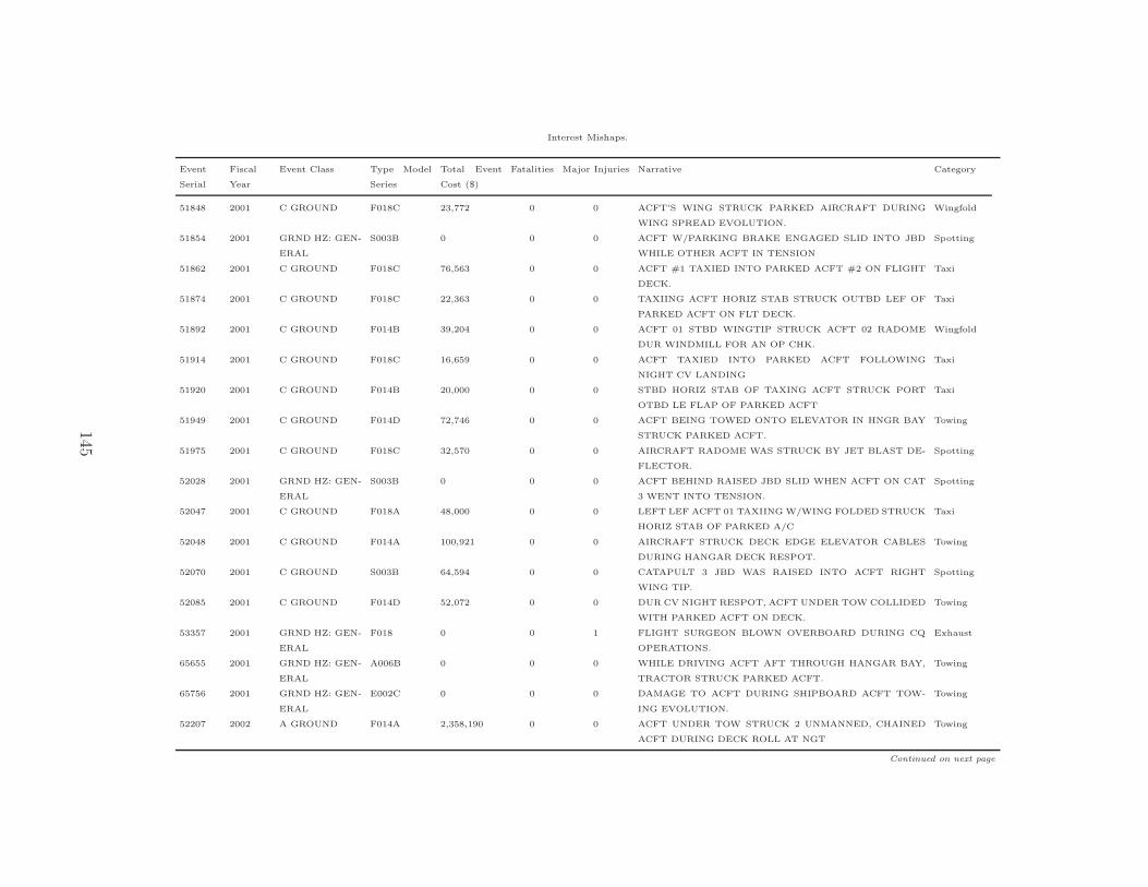
Interest Mishaps.

Event

Serial

Fiscal

Year

Event Class Type Model

Series

Total Event

Cost ($)

Fatalities Major Injuries Narrative Category

51848 2001 C GROUND F018C 23,772 0 0 ACFT’S WING STRUCK PARKED AIRCRAFT DURING

WING SPREAD EVOLUTION.

Wingfold

51854 2001 GRND HZ: GEN-

ERAL

S003B 0 0 0 ACFT W/PARKING BRAKE ENGAGED SLID INTO JBD

WHILE OTHER ACFT IN TENSION

Spotting

51862 2001 C GROUND F018C 76,563 0 0 ACFT #1 TAXIED INTO PARKED ACFT #2 ON FLIGHT

DECK.

Taxi

51874 2001 C GROUND F018C 22,363 0 0 TAXIING ACFT HORIZ STAB STRUCK OUTBD LEF OF

PARKED ACFT ON FLT DECK.

Taxi

51892 2001 C GROUND F014B 39,204 0 0 ACFT 01 STBD WINGTIP STRUCK ACFT 02 RADOME

DUR WINDMILL FOR AN OP CHK.

Wingfold

51914 2001 C GROUND F018C 16,659 0 0 ACFT TAXIED INTO PARKED ACFT FOLLOWING

NIGHT CV LANDING

Taxi

51920 2001 C GROUND F014B 20,000 0 0 STBD HORIZ STAB OF TAXING ACFT STRUCK PORT

OTBD LE FLAP OF PARKED ACFT

Taxi

51949 2001 C GROUND F014D 72,746 0 0 ACFT BEING TOWED ONTO ELEVATOR IN HNGR BAY

STRUCK PARKED ACFT.

Towing

51975 2001 C GROUND F018C 32,570 0 0 AIRCRAFT RADOME WAS STRUCK BY JET BLAST DE-

FLECTOR.

Spotting

52028 2001 GRND HZ: GEN-

ERAL

S003B 0 0 0 ACFT BEHIND RAISED JBD SLID WHEN ACFT ON CAT

3 WENT INTO TENSION.

Spotting

52047 2001 C GROUND F018A 48,000 0 0 LEFT LEF ACFT 01 TAXIING W/WING FOLDED STRUCK

HORIZ STAB OF PARKED A/C

Taxi

52048 2001 C GROUND F014A 100,921 0 0 AIRCRAFT STRUCK DECK EDGE ELEVATOR CABLES

DURING HANGAR DECK RESPOT.

Towing

52070 2001 C GROUND S003B 64,594 0 0 CATAPULT 3 JBD WAS RAISED INTO ACFT RIGHT

WING TIP.

Spotting

52085 2001 C GROUND F014D 52,072 0 0 DUR CV NIGHT RESPOT, ACFT UNDER TOW COLLIDED

WITH PARKED ACFT ON DECK.

Towing

53357 2001 GRND HZ: GEN-

ERAL

F018 0 0 1 FLIGHT SURGEON BLOWN OVERBOARD DURING CQ

OPERATIONS.

Exhaust

65655 2001 GRND HZ: GEN-

ERAL

A006B 0 0 0 WHILE DRIVING ACFT AFT THROUGH HANGAR BAY,

TRACTOR STRUCK PARKED ACFT.

Towing

65756 2001 GRND HZ: GEN-

ERAL

E002C 0 0 0 DAMAGE TO ACFT DURING SHIPBOARD ACFT TOW-

ING EVOLUTION.

Towing

52207 2002 A GROUND F014A 2,358,190 0 0 ACFT UNDER TOW STRUCK 2 UNMANNED, CHAINED

ACFT DURING DECK ROLL AT NGT

Towing

Continued on next page

145

Interest Mishaps.

Event

Serial

Fiscal

Year

Event Class Type Model

Series

Total Event

Cost ($)

Fatalities Major Injuries Narrative Category

52228 2002 C GROUND S003B 20,000 0 0 HANGAR BAY AMMUNITION ELEVATOR HATCH

OPENED AND STRUCK ACFT RADOME.

Spotting

52251 2002 C GROUND F018C 27,510 0 0 DURING ACFT TIEDOWN, OUTBD WING PYLON HIT

ADJACENT ACFT HORIZ STAB.

Towing

52361 2002 C GROUND F018E 125,318 0 0 ACFT1 STBD AILERON STRUCK ACFT2 STBD HORIZ

STAB DUR FLT DECK ACFT MOVE

Towing

52710 2002 C GROUND S003B 23,865 0 1 FLIGHT DECK TROUBLESHOOTER BLOWN DOWN ON

FLIGHT DECK BY ACFT EXHAUST.

Exhaust

52868 2002 C GROUND F014B 55,950 0 0 TOW TRACTOR IMPACTED STBD DROP TANK DURING

RESPOT EVOLUTION.

Towing

52953 2002 C GROUND F014B 20,000 0 0 ACFT UNDER TOW DURING FLIGHT DECK RESPOT

STRUCK BY NR 3 JBD.

Towing

52956 2002 C GROUND F018E 28,860 0 0 PORT HORIZ STAB DAMAGED BY ENGINE EXHAUST OF

LIKE ACFT DUR ENG START.

Exhaust

53356 2003 C GROUND F018C 22,940 0 0 AIRCRAFT SLID INTO ANOTHER AIRCRAFT DURING

CHOCKING & CHAINING.

Spotting

53395 2003 C GROUND SH060F 37,419 0 0 WHILE MOVING ACFT CRANE FOR FLT DECK DRILLS,

SLING HIT MRB AND TRB’S.

Misc

53403 2003 C GROUND F018E 179,580 0 0 AIRCRAFT #1 TAXIED INTO PARKED AIRCRAFT #2. Taxi

53447 2003 C GROUND F018E 90,268 0 0 STBD HORIZ STAB DAMAGED BY LANTERN POD ON

SKID BEING MOVED ON FLT DECK

Misc

53482 2003 C GROUND F018C 47,010 0 0 TOWED AIRCRAFT #1 BACKED INTO RADOME OF AIR-

CRAFT #2.

Towing

53692 2003 C GROUND F018C 134,760 0 0 WINDSHIELD DAMAGED AFTER EXPOSURE TO ACFT

ENG EXHAUST DUR LAUNCH CYCLE

Exhaust

53695 2003 B GROUND E002C+ 505,760 0 0 ACFT SLID INTO PARKED ACFT DAMAGING BOTH

ACFT & DEBRIS HIT 3RD ACFT.

Spotting

64733 2003 C GROUND EA006B 22,856 0 0 TOW TRACTOR IMPACTED BAND RADOME ON ACFT

STA WHILE TRYING TO TRANSIT.

Towing

64749 2003 C GROUND F018C 79,215 0 0 ACFT #1 TAXIED INTO ACFT #2 ON FLIGHT DECK. Taxi

64794 2003 B GROUND C002A 286,298 0 0 2 ACFT PARKED ON SHIP’S ELEVATOR DAMAGED DUR

ELEVATOR DOWNWARD TRAVEL.

Spotting

64851 2003 C FLIGHT F018A 22,021 0 0 AIRCRAFT #1 DAMAGED ON FLIGHT DECK WHEN IT

WAS TOWED INTO AIRCRAFT #2.

Towing

64852 2003 C GROUND F018C 64,610 0 0 ACFT #1 TAXIED INTO ACFT #2 ON FLIGHT DECK UN-

DER YELLOW SHIRT CONTROL.

Taxi

Continued on next page

146

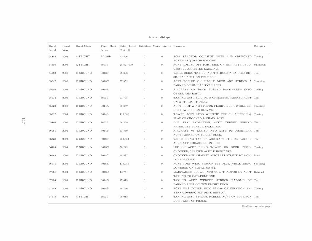
Interest Mishaps.

Event

Serial

Fiscal

Year

Event Class Type Model

Series

Total Event

Cost ($)

Fatalities Major Injuries Narrative Category

64855 2003 C FLIGHT EA006B 22,856 0 0 TOW TRACTOR COLLIDED WITH AND CRUNCHED

ACFT’S ALQ-99 POD RADOME.

Towing

64898 2003 A FLIGHT S003B 25,877,600 0 0 ACFT ROLLED OFF PORT SIDE OF SHIP AFTER SUC-

CESSFUL ARRESTED LANDING.

Unknown

64939 2003 C GROUND F018F 35,696 0 0 WHILE BEING TAXIED, ACFT STRUCK A PARKED DIS-

SIMILAR ACFT ON FLT DECK.

Taxi

65047 2003 C GROUND F018C 57,952 0 0 ACFT ROLLED ON FLIGHT DECK AND STRUCK A

PARKED DISSIMILAR TYPE ACFT.

Spotting

65193 2003 C GROUND F018A 0 0 0 AIRCRAFT ON DECK PUSHED BACKWARDS INTO

OTHER AIRCRAFT.

Towing

65614 2003 C GROUND S003B 21,755 0 0 TAXIING ACFT SLID INTO UNMANNED PARKED ACFT

ON WET FLIGHT DECK.

Taxi

65620 2003 C GROUND F014A 39,667 0 0 ACFT PORT WING STRUCK FLIGHT DECK WHILE BE-

ING LOWERED ON ELEVATOR.

Spotting

65717 2004 C GROUND F014A 113,682 0 0 TOWED ACFT STBD WINGTIP STRUCK AILERON &

FLAP OF CHOCKED & CHAIN ACFT.

Towing

65866 2004 C GROUND S003B 56,259 0 0 DUR TAXI EVOLUTION, ACFT TURNED BEHIND

RAISED JET BLAST DEFLECTOR.

Taxi

66061 2004 C GROUND F014B 73,350 0 0 AIRCRAFT #1 TAXIED INTO ACFT #2 DISSIMILAR

ACFT PARKED ON FLIGHT DECK.

Taxi

66328 2004 C GROUND F018F 263,551 0 0 WHILE BEING TAXIED, AIRCRAFT STRUCK PARKED

AIRCRAFT EMBARKED ON SHIP.

Taxi

66409 2004 C GROUND F018C 50,222 0 0 LEF OF ACFT BEING TOWED ON DECK STRUK

CHOCKED/CHAINED ACFT P HORIZ STB

Towing

66568 2004 C GROUND F018C 49,537 0 0 CHOCKED AND CHAINED AIRCRAFT STRUCK BY MOV-

ING FORKLIFT.

Misc

66975 2004 C GROUND F018E 138,056 0 0 ACFT PORT WING STRUCK FLT DECK WHILE BEING

LOWERED ON ELEVATOR #2.

Spotting

67061 2004 C GROUND F018C 1,875 0 0 MAINTAINER BLOWN INTO TOW TRACTOR BY ACFT

TAXIING TO CATAPULT ONE.

Exhaust

67103 2004 C GROUND F014B 27,673 0 0 TAXIING ACFT WINGTIP STRUCK RADOME OF

PARKED ACFT ON CVN FLIGHT DECK.

Taxi

67149 2004 C GROUND F014B 48,156 0 0 ACFT WAS TOWED INTO SPN-46 CALIBRATION AN-

TENNA DURING FLT DECK RESPOT.

Towing

67178 2004 C FLIGHT S003B 96,012 0 0 TAXIING ACFT STRUCK PARKED ACFT ON FLT DECK

DUR START-UP PHASE.

Taxi

Continued on next page

147

Interest Mishaps.

Event

Serial

Fiscal

Year

Event Class Type Model

Series

Total Event

Cost ($)

Fatalities Major Injuries Narrative Category

67255 2004 C GROUND F014B 27,673 0 0 ACFT RADOME DMG WHEN A PALLET JACK CARRY-

ING ISOPODS PULLED INTO RADOME

Misc

67423 2004 C GROUND F014B 47,673 0 0 TOWED AIRCRAFT WING STRUCK RADOME OF

PARKED ACFT ON SHIP FLIGHT DECK.

Towing

67595 2004 C GROUND E002C+ 25,944 0 0 PARKED HELO TAIL RTR STRUCK BY TAXIING FIXED

WING ACFT W/WING FOLDED.

Taxi

67604 2004 C GROUND F018F 63,632 0 0 ACFT BACKED INTO VERTICAL LIGHT FIXTURE DUR-

ING ACFT FLT DECK MOVE.

Towing

67605 2004 C GROUND T045C 351,008 0 0 JET BLAST DEFLECTOR STRUCK ACFT WHILE BEING

DIRECTED FOR CVN LAUNCH.

Taxi

68030 2004 C GROUND F018F 43,695 0 0 ACFT #1 WING PANEL IMPACTED ACFT #2 STABI-

LIZER DURING TAXI ONBOARD CVN

Taxi

68057 2004 C GROUND EA006B 23,464 0 0 ALQ-99 TACT JAMMING POD STRUCK BY TOW TRAC-

TOR ON CVN FLIGHT DECK.

Towing

68091 2004 C GROUND F018E 83,031 0 0 DUR TOW, ACFT’S PORT WING STRUCK STBD HORIZ

STABILATOR OF PARKED ACFT.

Towing

68160 2004 C GROUND E002C+ 182,189 0 0 AFT’S RUDDER TRIM TAB STRUCK STATIC P PROP OF

PARKED ACFT ON FLT DECK

Unknown

68161 2004 C GROUND F018E 0 0 0 DURING FLT DECK VERTREP, FORCKLIFT STRUCK

PORT HORIZ STAB OF PARKED AC

Misc

68369 2005 C FLTREL F018F 2,796 0 0 AS ACFT CAT LAUNCHED, IT’S CATM-9 FINS STRUCK

CATAPULT CREWMAN’S HEAD.

Contact

68370 2005 B GROUND F018C 115,000 0 1 SQN ACFT UNDER TOW DIRECTION OF YELLOW SHIRT

RAN OVR SHIP’S BLUE SHIRT

Contact

68480 2005 C FLIGHT MH053E 176,372 0 0 LDG ACFT’S DWNWASH BLEW PARKED ACFT’S RTR

BLADES INTO FLT DECK.

Exhaust

68506 2005 C GROUND F018E 51,760 0 0 ACFT AND TOW TRACTOR DAMAGED DUR ACFT

MOVE ON FLIGHT DECK. NO INJURIES

Towing

68707 2005 C FLTREL EA006B 25,630 0 0 ACFT’S TJS POD RADOME DAMAGED IN CVN HANGAR

BAY.

Unknown

69023 2005 C GROUND F018F 169,752 0 0 ACFT UNDER FLT DECK TAXI DIR CTRL STRUCK A

LIKE ACFT ON ELEVATOR FOUR.

Taxi

69123 2005 C GROUND HH060H 35,208 0 0 TOW TRACTOR STRUCK HELO TAIL PYLON PARKED

CHOCKED/CHAINED IN HELO HOLE

Towing

69133 2005 C GROUND F018C 35,699 0 0 AIRCRAFT UNDER TOW PUSHED BACK IN TO

NAVPOLE.

Towing

Continued on next page

148

Interest Mishaps.

Event

Serial

Fiscal

Year

Event Class Type Model

Series

Total Event

Cost ($)

Fatalities Major Injuries Narrative Category

69140 2005 C GROUND F018F 65,394 0 0 ACFT #1 STAB STRUCK PARKED ACFT #2 STBD

AILERON DUR TAXI FOR CV LAUNCH

Taxi

69153 2005 C GROUND F018F 63,500 0 0 STBD HORIZ STAB DAMAGED FM CONTACT WITH HYD

GEN DUR TOW TRACTOR MOVE.

Towing

69200 2006 C GROUND F018E 25,000 0 0 ACFT’S WING SPREAD INTO OTHER ACFT DAMAGING

RIGHT AILERON.

Wingfold

69202 2006 A GROUND T045C 1,050,699 0 0 AIRCRAFT ENGINE FOD BY INGESTION OF FLIGHT

DECK CREWMAN’S CRANIAL.

Engine

69213 2006 B GROUND F018C 115,000 0 1 ACFT RAN OVER AIRMAN’S RIGHT LEG DURING TAXI

ON FLIGHT DECK.

Contact

69270 2006 C GROUND F018F 38,767 0 0 EXT FUEL TANK DAMAGED FROM COLLISION WITH

TOW TRACTOR DURING ACFT TOW.

Towing

69279 2006 C GROUND F018E 46,400 0 0 ACFT TAXIED LEFT STABILATOR INTO STATIONARY

ACFT’S LEADING EDGE FLAP.

Taxi

69291 2006 C GROUND EA006B 95,058 0 0 ACFT UNDER FLT DECK TAXI DIR CONTROL TAXIED

INTO PARKED ACFT ON DECK.

Taxi

69310 2006 B GROUND F018F 368,328 0 0 RT WING OF ACFT #1 STRUCK THE L WING OF A

PARKED ACFT #2 DURING TAXI.

Taxi

69332 2006 C GROUND F018E 175,042 0 0 ACFT PARKED ON CV DECK DAMAGED BY ANOTHER

SQN’S LIKE ACFT JET EXHAUST.

Exhaust

69348 2006 C GROUND F018C 76,418 0 0 AIRCRAFT CANOPY DAMAGED BY ANOTHER AIR-

CRAFT’S EXHAUST.

Exhaust

69377 2006 C GROUND F018F 35,883 0 0 ACFT PARKED ON FLT DECK STRUCK BY FORK LIFT

TRACTOR DUR REPLENISHMENT.

Supply

69378 2006 C GROUND F018E 47,498 0 0 ACFT#1 TAXIED INTO ACFT#2 WHILE ACFT #2 WAS

STOPPED ON THE FLT DECK.

Taxi

69382 2006 C GROUND F018F 49,887 0 0 PARKED ACFT’S STBD HORIZ STAB DAMADED BY

TAXIING ACFT ON FLIGHT DECK.

Taxi

69385 2006 C GROUND F018F 122,406 0 0 TWO LIKE ACFT STRUCK EACH OTHER’S HORIZ STA-

BILIZER DUR FLT DECK TOWING

Towing

69415 2006 A GROUND S003 1,544,320 0 0 PORT STAB OF ACFT TAXIING STRUCK STBD TURN-

ING PROP OF PARKED ACFT.

Taxi, engine

69481 2007 C GROUND F018C 46,437 0 0 ACFT # 1 RIGHT STABILATOR WAS STRUCK BY ACFT

#2 LEFT STABILATOR.

Unknown

69504 2007 C GROUND F018E 61,203 0 0 GROUND SUPPORT EQUIPMENT STRUCK PORT HORI-

ZONTAL STABILATOR.

Unknown

Continued on next page

149

Interest Mishaps.

Event

Serial

Fiscal

Year

Event Class Type Model

Series

Total Event

Cost ($)

Fatalities Major Injuries Narrative Category

69517 2007 C GROUND F018E 23,996 0 0 A/C UNDER TOW DUR NIGHT RESPOT STBD STABILA-

TOR IMPACTED TOW TRACTOR.

Towing

69553 2007 C GROUND F018F 90,983 0 0 PORT AILERON OF ACFT UNDER TOW STRUCK PORT

HORZL STAB OF STA ACFT.

Towing

69566 2007 C GROUND EA006B 20,000 0 0 ALQ-99 POD RADOME DAMAGED ON FLT DECK. ACFT

RETURNED TO FLIGHT STATUS

Unknown

69590 2007 C GROUND F018F 74,096 0 0 PORT HORZL STABILATOR DAMGED ON ELEVATOR 4

STANCHION WHILE BEING TOWED

Towing

69602 2007 C GROUND F018F 23,936 0 0 ACFT SUSTAINED DAMAGE TO THE LEFT HRZL STAB

AFTER BEING TOWED.

Towing

69604 2007 C GROUND F018C 46,437 0 0 ACFT UNDER TOW ONBOARD SHIP STRUCK THE LDG

SIGNAL OFCR PLATFORM.

Towing

69607 2007 C GROUND F018F 151,220 0 0 JBD 3 WAS RAISED AND IMPACTED NG-111 WHILE UN-

DER TOW.

Towing

150

Appendix B. Source Code Listings

This appendix contains MATLABr and C source code used throughout this re-

search. It is provided as an example for future work.

B.1 MATLABr

Listing B.1: Determining time to calculate two-norms for different dimensions.1 %% LT Jeff Johnston

%

% 30 OCT 2008

% Determining time to calculate two -norms for different dimensions

6 clear all; close all; clc;

%% Generate times

max_dimension = 500;

11 max_runs = 1000;

times = zeros(max_dimension , max_runs);

for run_ctr = 1:1: max_runs

for ctr = 1:1: max_dimension

x = 1:1:ctr;

16 tic;

d = norm(x, 2);

times(ctr , run_ctr) = toc;

end

end

21

%% Get mean time of each operation

mean_times = zeros(size(times ,1) ,1);

for ctr = 1:1:size(times ,1)

26 mean_times(ctr) = mean(times(ctr ,:))*1E6;

end

%% Find a best -fit polynomial

31 p = polyfit(x’, mean_times , 3);

151

Listing B.2: DIDO Sample: Problem Definition.%% Example Script File for DIDO Path Planning Demonstration

% LT Jeff Johnston

% AFIT ENY

4 % 13JAN09

clear all; close all; clc;

%% Define OBSTACLES Variable (Structure)

9 global OBSTACLES;

% Each element of OBSTACLES structure is a nx1 column vector where...

n is the

% number of obstacles.

OBSTACLES.xo = [50]; % center location on x-axis

14 OBSTACLES.yo = [50]; % center location on y-axis

OBSTACLES.a = [10]; % width

OBSTACLES.b = [10]; % height

OBSTACLES.p = [2]; % norm: 1-diamond , 2-circle, 100-square, etc...

...

OBSTACLES.c = [1];

19

%% Define state and control parameter boundaries

xL = 0; xU = 100;

yL = 0; yU = 100;

psiL = -3*pi; psiU = 3*pi;

24

vL = 0; vU = 0.8;

phiL = -pi/2; phiU = pi/2;

bounds.lower.states = [xL; yL; psiL];

29 bounds.upper.states = [xU; yU; psiU];

bounds.lower.controls = [vL; phiL];

bounds.upper.controls = [vU; phiU];

34 t0 = 0;

tfMax = 500;

bounds.lower.time = [t0; t0];

bounds.upper.time = [t0; tfMax];

39

%% Define desired initial and final states

x0 = 0;

y0 = 0;

psi0 = -45*pi/180;

44

xf = 100;

yf = 100;

psif = -45*pi/180;

49 bounds.lower.events = [x0; y0; psi0; xf; yf; psif];

152

bounds.upper.events = [x0; y0; psi0; xf; yf; psif];

bounds.lower.path = zeros(size(OBSTACLES.xo))+0;

bounds.upper.path = zeros(size(OBSTACLES.xo))+1000;

54

%% Assign necessary variables to structure

Project.cost = ’SampleCost’;

Project.dynamics = ’SampleDynamics’;

Project.events = ’SampleEvents’;

59 Project.path = ’SamplePath’;

Project.bounds = bounds;

%% Set DIDO Options

64

algorithm.mode = ’spectral’;

algorithm.nodes = [40];

%% Call DIDO

69 tStart= cputime;

[cost , primal, dual] = dido(Project , algorithm);

runTime = cputime -tStart

%% Create output variables from DIDO solution structures

74

x = primal.states (1,:);

y = primal.states (2,:);

psi = primal.states (3,:);

79 t = primal.nodes;

%% Plot the resultant path

figure;

hold;

84 plot(x, y, ’:o’);

for ctr = 1:1:length(OBSTACLES.xo)

ezplot(strcat(’((x-’,num2str(OBSTACLES.xo(ctr)) ,...

’)/’,num2str(OBSTACLES.a(ctr)) ,...

’)^’,num2str(OBSTACLES.p(ctr)) ,...

89 ’+ ((y-’, num2str(OBSTACLES.yo(ctr)) ,...

’)/’,num2str(OBSTACLES.b(ctr)) ,...

’)^’,num2str(OBSTACLES.p(ctr)) ,...

’-’, num2str(OBSTACLES.c(ctr))) ,...

[xL , xU , yL, yU]);

94 end

axis([xL , xU , yL, yU]);

grid on;

xlabel(’x’);

ylabel(’y’);

99 title(’’);

153

Listing B.3: DIDO Sample: Events.1 function endpointFunction = ProjectEvents(primal)

% Event function for DIDO Path Planning Demonstration

% LT Jeff Johnston

% AFIT ENY

% 13JAN09

6

x0 = primal.states (1,1); xf = primal.states(1,end);

y0 = primal.states (2,1); yf = primal.states(2,end);

psi0 = primal.states (3,1); psif = primal.states (3,end);

11

endpointFunction = zeros(6,1);

endpointFunction(1) = x0;

endpointFunction(2) = y0;

endpointFunction(3) = psi0;

16 endpointFunction(4) = xf;

endpointFunction(5) = yf;

endpointFunction(6) = psif;

154

Listing B.4: DIDO Sample: Path.function pathFunction = ProjectPath(primal)

2 % Path constraint function for DIDO Path Planning Demonstration

% LT Jeff Johnston

% AFIT ENY

% 13JAN09

7 global OBSTACLES;

x = primal.states (1,:);

y = primal.states (2,:);

12 % Allow a border around the obstacle

border = 0.5; % m

xo = OBSTACLES.xo;

yo = OBSTACLES.yo;

17 a = OBSTACLES.a + border;

b = OBSTACLES.b + border;

p = OBSTACLES.p;

for ctr = 1:1:length(xo)

22 pathFunction(ctr ,:) = log(((x-xo(ctr))./(a(ctr))).^p(ctr) +...

((y-yo(ctr))./(b(ctr))).^p(ctr));

end

155

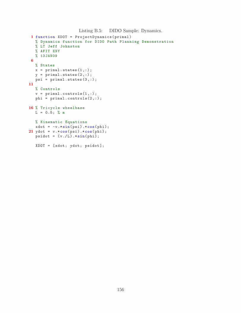
Listing B.5: DIDO Sample: Dynamics.1 function XDOT = ProjectDynamics(primal)

% Dynamics function for DIDO Path Planning Demonstration

% LT Jeff Johnston

% AFIT ENY

% 13JAN09

6

% States

x = primal.states (1,:);

y = primal.states (2,:);

psi = primal.states (3,:);

11

% Controls

v = primal.controls(1,:);

phi = primal.controls(2,:);

16 % Tricycle wheelbase

L = 0.5; % m

% Kinematic Equations

xdot = -v.*sin(psi).*cos(phi);

21 ydot = v.*cos(psi).*cos(phi);

psidot = (v./L).*sin(phi);

XDOT = [xdot; ydot; psidot ];

156

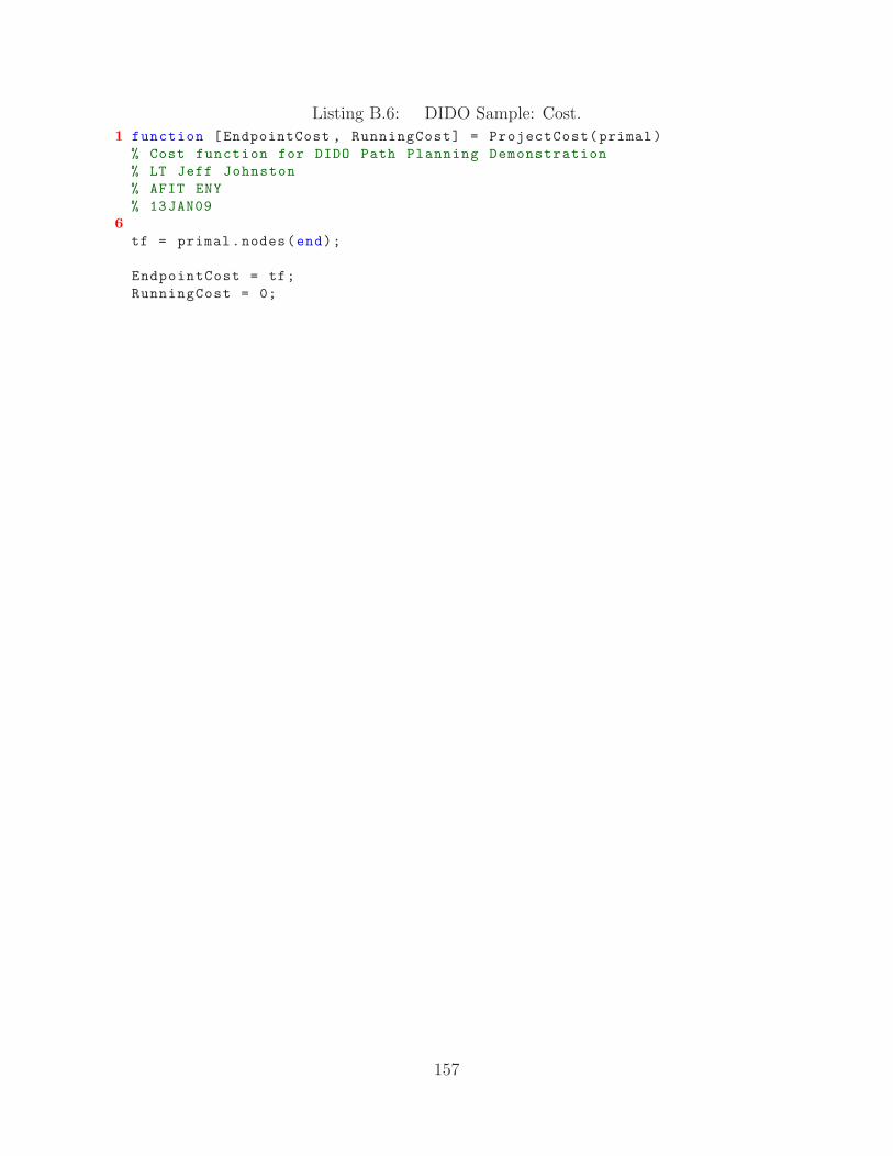
Listing B.6: DIDO Sample: Cost.1 function [EndpointCost , RunningCost] = ProjectCost(primal)

% Cost function for DIDO Path Planning Demonstration

% LT Jeff Johnston

% AFIT ENY

% 13JAN09

6

tf = primal.nodes(end);

EndpointCost = tf;

RunningCost = 0;

157

Listing B.7: Determine vehicle position and orientation from measured antennalocations.

function [ rc, heading ] = det_pos_heading( r1, r2 )

%DET_POS_HEADING Returns center position and heading from wingtip

%coordinates

%

5 % LT Jeff Johnston

% AFIT/ENY

% 21OCT2008

%

%Usage: [rc, heading] = det_pos_heading( r1 , r2 )

10 %

% r1: 1x2 vector containing coordinates of port receiver [x_1 , ...

y_1]

% r2: 1x2 vector containing coordinates of stbd receiver [x_2 , ...

y_2]

%

% rc: Returns 1x2 vector containing coordinates of center [x_c , ...

y_c]

15 % heading: Returns angle from north in degrees

r3 = r2 - r1;

L = norm(r3);

20 heading = atan2(r3(2), r3(1));

rc = r1+(L/2)*[cos(heading), sin(heading)];

heading = heading*180/ pi;

158

Listing B.8: Calculate nearest neighbor distance.function [ dist ] = dist_from_object( loc , rc , heading , threshold ,...

wingspan , object )

%[ dist ] = DIST_FROM_OBJECT ( loc , rc , heading)

3 %Calculates the distance of a point from an object described by a ...

patch

%

% LT Jeff Johnston

% AFIT/ENY

% 29OCT2008

8 %

% loc: 1x2 vector containing coordinates of point [x, y]

% rc: 1x2 vector containing coordinates of object center point [...

x_c , y_c]

% heading: object angle from heading north (in degrees)

% threshold: minimum safe distance from center of object

13 % wingspan: length of wingspan tip -to -tip

% object: string containing file name of object outline

% First let ’s just try calculating the distance to the center ...

point

dist = norm(rc -loc);

18

% If the distance to the center is less than the threshold given , ...

use the

% nearest neighbor method

if dist < threshold

% Load object outline and apply coordinate transformations

23 load(object);

heading_rad = -heading*pi/180;

scaling = wingspan / ( 2 * max(outline(:,1)));

object_outline = outline*[cos(heading_rad) ,...

-sin(heading_rad); sin(heading_rad) cos( heading_rad)];

28 shifting_points = zeros(size(object_outline));

for ctr = 1:1:size(shifting_points ,1)

shifting_points(ctr ,:) = rc;

end

33 object_outline = object_outline*scaling + shifting_points;

% BRUTE FORCE NEAREST NEIGHBOR

temp_dist = zeros(size(object_outline , 1) ,1);

for ctr = 1:1:size(object_outline , 1)

38 temp_dist(ctr) = norm(loc -object_outline(ctr ,:));

end

dist = min(temp_dist);

end

159

Listing B.9: DIDO Aircraft Towing Problem: Problem Definition.%% Problem file for the Aircraft Towing Problem

% LT Jeff Johnston , USN

3 % Lt. Col. Eric Swenson , USAF

% AFIT ENY

% 15JAN09

%

% Adapted from files provided by CDR Michael Hurni , USN , NPS

8

clear all; close all; clc;

path(path ,’../scripts’);

%% Define Global Variables

13

global LC LB LA OBSTACLES X;

% Global Scaling Factor

% Location states need scaling to be closer to order of magnitude ...

of other

18 % states

X = 50;

% Articulated Vehicle Dimensions

% Dimensions in meters, scaled by X

23 LC = 3/X; % Tow Tractor Wheel Base Length

LB = 5/X; % Tow Bar Length

LA = 8/X; % Aircraft Wheel Base Length

% Measured Data Plotting Switch

28 % When plot_meas_data==1 the measured data recorded at NAS Oceana ...

will be

% plotted with the planned path.

plot_meas_data = 1;

% Measured Data Guess Switch

33 % When guess_meas_data==1 the measured data recorded at NAS Oceana...

will be

% used to provide an initial guess for the DIDO solution.

guess_meas_data = 1;

guess_start_end = 0;

38

% Measured Data Guess Plotting Switch

% When plot_guess_meas_data ==1 the guess generated from the ...

measured data

% recorded at NAS Oceana will be plotted to all for verification

plot_guess_meas_data = 1;

43

% Animate Optimal Solution

% When animate_soln==1 the resultant path will be animated

animate_soln = 0;

160

48 % Rotate Axes

T = [ cosd(48) -sind(48) ;sind(48) cosd(48)];

% Obstacle Locations and Configurations

OBSTACLES.xo = [ 81.0362; 140.2932; 103.8932; 116.8932; 90.8932; ...

77.8932; 64.8932; 51.8932; 50; 20]/X;

53 OBSTACLES.yo = [109.2882; 100.8977; 64.4977; 77.4977; 51.4977; ...

38.4977; 25.4977; 12.4977; 100; 100]/X;

rotated_OBSTACLES = [OBSTACLES.xo OBSTACLES.yo]*T;

OBSTACLES.xo = rotated_OBSTACLES(:,1);

OBSTACLES.yo = rotated_OBSTACLES(:,2);

OBSTACLES.a = [ 14; 14; 14; 14; 14; ...

14; 10; 10; 15; 10]/X; % width

58 OBSTACLES.b = [ 22; 22; 22; 22; 22; ...

22; 10; 10; 15; 10]/X; % height

OBSTACLES.p = [ 4; 4; 4; 4; 4; ...

4; 2; 2; 2; 2];

OBSTACLES.c = [ 1; 1; 1; 1; 1; ...

1; 1; 1; 1; 1];

OBSTACLES.border = 0.5/X;

OBSTACLES.d_des = 20/X;

63 OBSTACLES.idx = [1 2 3 4 5];

% Obstacle On/Off Switch

% When OBSTACLES.switch ==1 the obstacles will be present in the ...

path

% planning scenario

68 OBSTACLES.switch = 1;

%% Bound State and Control Variables

%

% The states for this problem are as follows (14):

73 % xc: Tow Tractor Horizontal Location (c stands for cart)

% yc: Tow Tractor Vertical Location

% beta_s

% beta_c: SIN and COS of Tow Tractor Heading Relative to ...

Horizontal

% xw: Nose Wheel Horizontal Location (w stands for wheel)

78 % yw: Nose Wheel Vertical Location

% theta_s

% theta_c: SIN and COS of Tow Bar Heading Relative to ...

Horizontal

% zeta: Tow Bar Turn Angle , beta -theta

% xa: Aircraft Horizontal Location (a stands for aircraft)

83 % ya: Aircraft Vertical Location

% psi_s

% psi_c: SIN and COS of Aircraft Heading Relative to ...

Horizontal

% phi: Aircraft Turn Angle , theta -psi

%

88 % The controls for this problem are as follow (2):

% vc: Tow Tractor Velocity

161

% alpha: Tow Tractor Turn Angle

%

% All angles in radians

93 % All distances in meters scaled by X

% All velocities in meters/second scaled by X

% Lower and Upper Bounds for Locations

xmin = 50/X; xmax = 200/X; ymin = -200/X; ymax = 59/X;

98 xcL = xmin; xcU = xmax; xwL = xmin; xwU = xmax; xaL = xmin; xaU = ...

xmax;

ycL = ymin; ycU = ymax; ywL = ymin; ywU = ymax; yaL = ymin; yaU = ...

ymax;

% Lower and Upper Bounds for Headings

% -1 <= SIN(*), COS(*) <= 1, for all *

103 beta_sL = -1; beta_sU = 1;

beta_cL = -1; beta_cU = 1;

theta_sL = -1; theta_sU = 1;

theta_cL = -1; theta_cU = 1;

psi_sL = -1; psi_sU = 1;

108 psi_cL = -1; psi_cU = 1;

% Lower and Upper Bounds for Turn Angles

turn_angle_max = 4*pi/8;

zetaL = -turn_angle_max; zetaU = turn_angle_max;

113 phiL = -turn_angle_max; phiU = turn_angle_max;

% Lower and Upper Bounds for Inputs

vcL = 0/X; vcU = 0.5/X;

alphaL = -pi/2; alphaU = pi/2;

118

bounds.lower.states = [xcL; ycL; beta_sL; beta_cL; xwL; ywL; ...

theta_sL; theta_cL; zetaL; xaL; yaL; psi_sL; psi_cL; phiL];

bounds.upper.states = [xcU; ycU; beta_sU; beta_cU; xwU; ywU; ...

theta_sU; theta_cU; zetaU; xaU; yaU; psi_sU; psi_cU; phiU];

bounds.lower.controls = [vcL; alphaL ];

123 bounds.upper.controls = [vcU; alphaU ];

%% Bound the Initial and Final Times

t0 = 0;

128 tfMax = 600;

bounds.lower.time = [t0; t0];

bounds.upper.time = [t0; tfMax];

133 %% Set the Initial and Final Conditions

% Measured Start Location of Aircraft

xa0 = 129.2289/X;

ya0 = 89.8569/X;

162

138 rotated_xy0 = [xa0 ya0]*T;

xa0 = rotated_xy0(1);

ya0 = rotated_xy0(2);

psi0 = ( -130.6658+90 -48)*pi/180;

% xa0 = 0;

143 % ya0 = 50/X;

% psi0 = 0;

psi_s0 = sin(psi0);

psi_c0 = cos(psi0);

148

% Calculated Start Location of Nose Wheel (and Tow Bar)

xw0 = xa0+LA*cos(psi0);

yw0 = ya0+LA*sin(psi0);

theta0 = psi0;

153 theta_s0 = sin(theta0);

theta_c0 = cos(theta0);

phi0 = theta0-psi0;

% Calculated Start Location of Tow Tractor

158 xc0 = xw0+LB*cos(theta0);

yc0 = yw0+LB*sin(theta0);

beta0 = psi0;

beta_s0 = sin(beta0);

beta_c0 = cos(beta0);

163 zeta0 = beta0 -theta0;

% Measured Final Location of Aircraft

xaf = 29.0362/X;

yaf = 57.2882/X;

168 rotated_xyf = [xaf yaf]*T;

xaf = rotated_xyf(1);

yaf = rotated_xyf(2);

psif = (49.2842+90-48)*pi/180;

% xaf = 100/X;

173 % yaf = 150/X;

% psif = 0;

psi_sf = sin(psif);

psi_cf = cos(psif);

178

% Calculated Final Location of Nose Wheel (and Tow Bar)

xwf = xaf+LA*cos(psif);

ywf = yaf+LA*sin(psif);

thetaf = psif;

183 theta_sf = sin(thetaf);

theta_cf = cos(thetaf);

phif = thetaf -psif;

% Calculated Final Location of Tow Tractor

188 xcf = xwf+LB*cos(thetaf);

ycf = ywf+LB*sin(thetaf);

163

betaf = psif;

beta_sf = sin(betaf);

beta_cf = cos(betaf);

193 zetaf = betaf -thetaf;

% Upper and Lower Boundaries for Initial and Final States

%

% Force aircraft to attain its exact final state but allows cart ...

and tow bar

198 % to be at an offset. DIDO requires [2*n x 1] column vector where...

n is the

% number of states.

%

% Define maximum allowable offsets

x_off = 5/X;

203 y_off = 5/X;

a_off = pi/8;

sc_off = 0.4;

%

% Create bounds vector

208 bounds.lower.events = [xc0; yc0; beta_s0; beta_c0; xw0; yw0; ...

theta_s0; theta_c0; zeta0; xa0; ya0; psi_s0; psi_c0; phi0; xcf -...

x_off; ycf -x_off; beta_sf -sc_off; beta_cf -sc_off; xwf; ywf; ...

theta_sf -sc_off; theta_cf -sc_off; zetaf -a_off; xaf; yaf; psi_sf...

; psi_cf; phif -a_off];

bounds.upper.events = [xc0; yc0; beta_s0; beta_c0; xw0; yw0; ...

theta_s0; theta_c0; zeta0; xa0; ya0; psi_s0; psi_c0; phi0; xcf+...

y_off; ycf+y_off; beta_sf+sc_off; beta_cf+sc_off; xwf; ywf; ...

theta_sf+sc_off; theta_cf+sc_off; zetaf+a_off; xaf; yaf; psi_sf...

; psi_cf; phif+a_off];

% bounds.lower.events = [xc0; yc0; beta_s0; beta_c0; xw0; yw0; ...

theta_s0; theta_c0; zeta0; xa0; ya0; psi_s0; psi_c0; phi0; xcf;...

ycf; beta_sf; beta_cf; xwf; ywf; theta_sf; theta_cf; zetaf; ...

xaf; yaf; psi_sf; psi_cf; phif];

% bounds.upper.events = [xc0; yc0; beta_s0; beta_c0; xw0; yw0; ...

theta_s0; theta_c0; zeta0; xa0; ya0; psi_s0; psi_c0; phi0; xcf;...

ycf; beta_sf; beta_cf; xwf; ywf; theta_sf; theta_cf; zetaf; ...

xaf; yaf; psi_sf; psi_cf; phif];

213

bounds.lower.path = zeros(length(OBSTACLES.idx), 1)+0;

bounds.upper.path = zeros(length(OBSTACLES.idx), 1)+100;

%% Plot the Initial/Final Conditions

218 draw_switch = 1;

if draw_switch == 1;

figure;

hold on;

223 draw_aircraft([xa0*X, ya0*X], (psi0 -pi/2)*180/pi , 11.43 , ’...

fa18c’, ’g’);

164

draw_aircraft([xc0*X, yc0*X], (beta0 -pi/2)*180/pi , 4, ’cart’, ...

’w’);

plot([xw0*X xc0*X],[yw0*X yc0*X],’r’);

draw_aircraft([xaf*X, yaf*X], (psif -pi/2)*180/pi , 11.43 , ’...

fa18c’, ’g’);

228 draw_aircraft([xcf*X, ycf*X], (betaf -pi/2)*180/pi , 4, ’cart’, ...

’w’);

plot([xwf*X xcf*X],[ywf*X ycf*X],’r’);

meas_xy_rot = meas_xy*T;

233 if plot_meas_data == 1

plot(meas_xy_rot(1:3000 ,1), meas_xy_rot(1:3000 ,2), ’m-.’);

end

if OBSTACLES.switch == 1

238 for ctr = 1:1: length(OBSTACLES.idx)

ezplot(strcat(’((x-’,num2str(OBSTACLES.xo(OBSTACLES....

idx(ctr))*X) ,...

’)/’,num2str(OBSTACLES.a(OBSTACLES.idx(ctr))*X)...

,...

’)^’,num2str(OBSTACLES.p(OBSTACLES.idx(ctr))) ,...

’+ ((y-’, num2str(OBSTACLES.yo(OBSTACLES.idx(ctr))...

*X) ,...

243 ’)/’,num2str(OBSTACLES.b(OBSTACLES.idx(ctr))*X)...

,...

’)^’,num2str(OBSTACLES.p(OBSTACLES.idx(ctr))) ,...

’-’, num2str(OBSTACLES.c(OBSTACLES.idx(ctr)))) ,...

[ -200 ,200 , -200 ,200]);

end

248 end

title(’’);

xlabel(’x’);

ylabel(’y’);

253 axis([55 205 -95 55]);

grid on;

end

%% Define DIDO Constraints

258

Project.cost = ’ProjectCost’;

Project.dynamics = ’ProjectDynamics’;

Project.events = ’ProjectEvents’;

Project.path = ’ProjectPath’;

263

Project.bounds = bounds;

%% Provide a Trajectory Guess

268 if guess_meas_data==1

165

load meas_data.mat;

meas_xy = meas_xy*T;

meas_hdg = meas_hdg+90 -48;

273

% Indices of measured data to use for guess generation

idx_use = [1; 1320; 1520; 1620; 1920; 2120; 2220; 3000];

idx_start = 800;

guess.controls = zeros(2,length(idx_use));

278 guess.states = zeros (14, length(idx_use));

guess.time = zeros(1,length(idx_use));

for ctr = 1:1:length(idx_use)

guess.controls(:,ctr) = [vcU; 0];

guess.states (10,ctr) = meas_xy(idx_use(ctr), 1)/X;

283 guess.states (11,ctr) = meas_xy(idx_use(ctr), 2)/X;

guess.states (12,ctr) = sin((meas_hdg(idx_use(ctr)))*pi...

/180);

guess.states (13,ctr) = cos((meas_hdg(idx_use(ctr)))*pi...

/180);

guess.states (14,ctr) = 0;

guess.states(5, ctr) = guess.states (10,ctr)+LA*guess....

states (13,ctr);

288 guess.states(6, ctr) = guess.states (11,ctr)+LA*guess....

states (12,ctr);

guess.states(7, ctr) = guess.states (12,ctr);

guess.states(8, ctr) = guess.states (13,ctr);

guess.states(9, ctr) = guess.states (14,ctr);

guess.states(1, ctr) = guess.states (5, ctr)+LB*guess....

states (8, ctr);

293 guess.states(2, ctr) = guess.states (6, ctr)+LB*guess....

states (7, ctr);

guess.states(3, ctr) = guess.states (7, ctr);

guess.states(4, ctr) = guess.states (8, ctr);

guess.time(ctr) = (ctr -1)*500/ length(idx_use);

end

298 algorithm.guess = guess;

if plot_guess_meas_data ==1

hold on;

for ctr = 1:1: length(idx_use)

303 draw_aircraft([guess.states (10,ctr)*X, guess.states...

(11,ctr)*X], (meas_hdg(idx_use(ctr)) -90), 11.43 , ’...

fa18c’, ’g’);

draw_aircraft([guess.states (1, ctr)*X, guess.states(2,...

ctr)*X], (meas_hdg(idx_use(ctr)) -90), 4, ’cart’, ’...

w’);

plot([guess.states(5, ctr)*X guess.states(1, ctr)*X],[...

guess.states (6, ctr)*X guess.states (2, ctr)*X],’r’)...

;

plot(meas_xy(1:3000 ,1), meas_xy(1:3000 ,2), ’m-.’);

166

text(guess.states (1, ctr)*X,guess.states (2, ctr)*X,...

strcat(’t=’,num2str(guess.time(ctr))),’FontSize’...

,10,’FontName’,’Arial’);

308 text(guess.states (1, ctr)*X,guess.states (2, ctr)*X-5,...

strcat(’hdg=’,num2str(meas_hdg(idx_use(ctr)))),’...

FontSize’,10,’FontName’,’Arial’);

end

title(’Measured Data and Generated Guesses’);

xlabel(’x’);

ylabel(’y’);

313 end

end

if guess_start_end == 1

guess.controls = [vcU vcU; 0 0];

318 guess.states (:,1) = [xc0; yc0; beta_s0; beta_c0; xw0; yw0; ...

theta_s0; theta_c0; zeta0; xa0; ya0; psi_s0; psi_c0; phi0];

guess.states (:,2) = [xcf; ycf; beta_sf; beta_cf; xwf; ywf; ...

theta_sf; theta_cf; zetaf; xaf; yaf; psi_sf; psi_cf; phif];

guess.time = [0 tfMax];

algorithm.guess = guess;

end

323

%% Set DIDO Run Options

algorithm.mode = ’spectral’;

328 % Number of Nodes

algorithm.nodes = 50;

%% Execute DIDO

333 tStart= cputime; % start CPU clock

[cost , primal, dual] = dido(Project , algorithm);

runTime = cputime -tStart;

disp(strcat(’Run Time is: ’, num2str(runTime)));

338 %% Store Trajectory Results

% Define the States for Readability

xc = primal.states (1,:)*X;

yc = primal.states (2,:)*X;

343 beta_s = primal.states (3,:);

beta_c = primal.states (4,:);

xw = primal.states (5,:)*X;

yw = primal.states (6,:)*X;

theta_s = primal.states (7,:);

348 theta_c = primal.states (8,:);

zeta = primal.states (9,:);

xa = primal.states (10 ,:)*X;

ya = primal.states (11 ,:)*X;

psi_s = primal.states (12 ,:);

167

353 psi_c = primal.states (13 ,:);

phi = primal.states (14 ,:);

% Define the Controls for Readability

vc = primal.controls(1,:)*X;

358 alpha = primal.controls(2,:);

% Resolve Angles Stored as SIN and COS

beta = atan2(beta_s, beta_c);

theta = atan2(theta_s , theta_c);

363 psi = atan2(psi_s , psi_c);

% Define the Time Vector

t = primal.nodes;

368 save kinematics.mat;

%% Plot Resultant Path

figure;

373 hold on;

draw_aircraft([xa0*X, ya0*X], (psi0 -pi/2)*180/pi , 11.43 , ’fa18c’, ...

’g’);

draw_aircraft([xaf*X, yaf*X], (psif -pi/2)*180/pi , 11.43 , ’fa18c’, ...

’g’);

378

if OBSTACLES.switch == 1

for ctr = 1:1:length(OBSTACLES.idx)

ezplot(strcat(’((x-’,num2str(OBSTACLES.xo(OBSTACLES.idx(...

ctr))*X) ,...

’)/’,num2str(OBSTACLES.a(OBSTACLES.idx(ctr))*X) ,...

383 ’)^’,num2str(OBSTACLES.p(OBSTACLES.idx(ctr))) ,...

’+ ((y-’, num2str(OBSTACLES.yo(OBSTACLES.idx(ctr))*X)...

,...

’)/’,num2str(OBSTACLES.b(OBSTACLES.idx(ctr))*X) ,...

’)^’,num2str(OBSTACLES.p(OBSTACLES.idx(ctr))) ,...

’-’, num2str(OBSTACLES.c(OBSTACLES.idx(ctr)))) ,...

388 [ -200 ,200 , -200 ,200]);

if OBSTACLES.idx(ctr) == 1

draw_aircraft([ OBSTACLES.xo(OBSTACLES.idx(ctr))*X, ...

OBSTACLES.yo(OBSTACLES.idx(ctr))*X], (psif -pi/2)...

*180/pi , 11.43 , ’fa18c’, ’w’);

else

draw_aircraft([ OBSTACLES.xo(OBSTACLES.idx(ctr))*X, ...

OBSTACLES.yo(OBSTACLES.idx(ctr))*X], (psi0 -pi/2)...

*180/pi , 11.43 , ’fa18c’, ’w’);

393 end

end

end

168

if plot_meas_data == 1

398 plot( meas_xy_rot(1:3000 ,1), meas_xy_rot(1:3000 ,2), ’m-.’);

end

axis([55 205 -95 55]);

xlabel(’x’);

403 ylabel(’y’);

title(’’);

grid on;

print -depsc -r300 ’~/ Documents/workspace/AFIT Thesis/src/Chapter4...

/img/mlplot_naso_path_planning_1.eps’;

408 for ctr = 1:1:length(xa)

draw_aircraft([xa(ctr), ya(ctr)], (psi(ctr)-pi/2)*180/pi, ...

11.43 , ’fa18c’, ’g’);

draw_aircraft([xc(ctr), yc(ctr)], (beta(ctr)-pi/2)*180/pi , 4, ...

’cart’, ’w’);

plot([xw(ctr) xc(ctr)],[yw(ctr) yc(ctr)],’r’);

end

413

plot(xa, ya ,’-o’);

plot(xw, yw ,’b*’);

plot(xc, yc ,’rx’);

print -depsc -r300 ’~/ Documents/workspace/AFIT Thesis/src/Chapter4...

/img/mlplot_naso_path_planning_3.eps’;

418

xlabel(’X-axis (m)’);

ylabel(’Y-axis (m)’);

title(’Vehicle Trajectory’);

423 %% Plot the states vs. time

%Plot the states and controls vs time

figure;

subplot(2,1,1); plot(t, xa, ’-o’, t, ya, ’-x’);

428 title(’Aircraft Postion’);

xlabel(’time (s)’);

ylabel(’x-y position’);

legend(’x (m)’, ’y (m)’);

grid;

433 subplot(2,1,2); plot(t, psi*180/pi, ’-ro’);

title(’Aircraft Angle From Global Y-Axis’);

xlabel(’time (s)’);

ylabel(’states ’);

legend(’\psi (deg)’);

438 grid;

%

%Plot the hamiltonian vs time

figure;

plot(t, dual.Hamiltonian , ’-o’);

443 title(’Hamiltonian Evolution’);

xlabel(’time (s)’);

169

ylabel(’Hamiltonian Value’);

grid;

448 %Plot the costates

figure;

plot(t, dual.dynamics(1,:), ’-o’ ,...

t, dual.dynamics(2,:), ’-x’ ,...

t, dual.dynamics(3,:), ’-.’ ,...

453 t, dual.dynamics(4,:), ’-+’ ,...

t, dual.dynamics(5,:), ’-x’ ,...

t, dual.dynamics(6,:), ’-.’ ,...

t, dual.dynamics(7,:), ’-+’ ,...

t, dual.dynamics(8,:), ’-x’ ,...

458 t, dual.dynamics(9,:), ’-.’ ,...

t, dual.dynamics(10 ,:), ’-+’ ,...

t, dual.dynamics(11 ,:), ’-x’ ,...

t, dual.dynamics(12 ,:), ’-.’ ,...

t, dual.dynamics(13 ,:), ’-+’ ,...

463 t, dual.dynamics(14 ,:), ’-*’);

title(’Costates’);

xlabel(’time (s)’);

ylabel(’costates’);

legend(’\lambda_x’, ’\lambda_y’, ’\lambda_\theta’, ’\lambda_v_r’, ...

’\lambda_v_l’);

468 grid;

%Plot the state covectors

figure;

plot(t, dual.states (1,:), ’-o’ ,...

473 t, dual.states (2,:), ’-x’ ,...

t, dual.states (3,:), ’-.’ ,...

t, dual.states (4,:), ’-+’ ,...

t, dual.states (5,:), ’-x’ ,...

t, dual.states (6,:), ’-.’ ,...

478 t, dual.states (7,:), ’-+’ ,...

t, dual.states (8,:), ’-x’ ,...

t, dual.states (9,:), ’-.’ ,...

t, dual.states (10 ,:), ’-+’ ,...

t, dual.states (11 ,:), ’-x’ ,...

483 t, dual.states (12 ,:), ’-.’ ,...

t, dual.states (13 ,:), ’-+’ ,...

t, dual.states (14 ,:), ’-*’);

title(’State covectors’);

xlabel(’time (s)’);

488 ylabel(’state covectors’);

legend(’\mu_x’, ’\mu_y’, ’\mu_\theta’, ’\mu_v_r ’, ’\mu_v_l ’);

grid;

%Plot the control covectors

493 figure;

plot(t, dual.controls(1,:)./4, ’-o’, t, dual.controls(2,:)./4, ’-x...

’);

170

title(’Control Covectors’);

xlabel(’time (s)’);

ylabel(’control covectors’);

498 legend(’\mu_a_r ’, ’\mu_a_l ’);

grid;

%Plot the Path covectors

figure;

503 plot(t, dual.path(1,:), ’-o’);

title(’Path Covectors’);

xlabel(’time (s)’);

ylabel(’path covectors’);

legend(’\mu_h_1 ’);

508

%Plot the Controls vs time

figure;

subplot(2,1,1); plot(t, vc, ’-o’);

%legend(’v (m/s) ’);

513 title(’Controls - Velocity of Cart’);

xlabel(’time (s)’);

ylabel(’v (m/s)’);

subplot(2,1,2); plot(t, alpha *180/pi , ’-x’);

title(’Controls - Steering angle \alpha’);

518 xlabel(’time (s)’);

ylabel(’alpha (deg)’);

grid;

%% Animate the Solution

523

if animate_soln==1

draw_DIDO_soln;

end

171

Listing B.10: DIDO Aircraft Towing Problem: Events.function endpointFunction = ProjectEvents(primal)

% Event file for the Aircraft Towing Problem

% LT Jeff Johnston , USN

4 % Lt. Col. Eric Swenson , USAF

% AFIT ENY

% 15JAN09

%

% Adapted from files provided by CDR Michael Hurni , USN , NPS

9

% Designate the Initial and Final States

xc0 = primal.states (1,1); xcf = primal.states(1,end);

yc0 = primal.states (2,1); ycf = primal.states(2,end);

beta_s0 = primal.states (3,1); beta_sf = primal.states(3, end);

14 beta_c0 = primal.states (4,1); beta_cf = primal.states(4, end);

xw0 = primal.states (5,1); xwf = primal.states(5,end);

yw0 = primal.states (6,1); ywf = primal.states(6,end);

theta_s0 = primal.states (7,1); theta_sf = primal.states(7,end);

theta_c0 = primal.states (8,1); theta_cf = primal.states(8,end);

19 zeta0 = primal.states (9,1); zetaf = primal.states(9,end);

xa0 = primal.states (10 ,1); xaf = primal.states (10,end);

ya0 = primal.states (11 ,1); yaf = primal.states (11,end);

psi_s0 = primal.states (12 ,1); psi_sf = primal.states (12,end);

psi_c0 = primal.states (13 ,1); psi_cf = primal.states (13,end);

24 phi0 = primal.states (14 ,1); phif = primal.states (14,end);

% Put the Initial and Final States in endpointFunction

% Pre -allocate endpointFunction

29 endpointFunction = zeros (28 ,1);

% Initial Conditions

endpointFunction(1) = xc0;

endpointFunction(2) = yc0;

34 endpointFunction(3) = beta_s0;

endpointFunction(4) = beta_c0;

endpointFunction(5) = xw0;

endpointFunction(6) = yw0;

endpointFunction(7) = theta_s0;

39 endpointFunction(8) = theta_c0;

endpointFunction(9) = zeta0;

endpointFunction(10) = xa0;

endpointFunction(11) = ya0;

endpointFunction(12) = psi_s0;

44 endpointFunction(13) = psi_c0;

endpointFunction(14) = phi0;

% Final Conditions

endpointFunction(15) = xcf;

49 endpointFunction(16) = ycf;

endpointFunction(17) = beta_sf;

endpointFunction(18) = beta_cf;

172

endpointFunction(19) = xwf;

endpointFunction(20) = ywf;

54 endpointFunction(21) = theta_sf;

endpointFunction(22) = theta_cf;

endpointFunction(23) = zetaf;

endpointFunction(24) = xaf;

endpointFunction(25) = yaf;

59 endpointFunction(26) = psi_sf;

endpointFunction(27) = psi_cf;

endpointFunction(28) = phif;

173

Listing B.11: DIDO Aircraft Towing Problem: Path.function pathFunction = ProjectPath(primal)

% Path file for the Aircraft Towing Problem

% LT Jeff Johnston , USN

4 % Lt. Col. Eric Swenson , USAF

% AFIT ENY

% 15JAN09

%

% Adapted from files provided by CDR Michael Hurni , USN , NPS

9

% Load Global Variables

global OBSTACLES;

if OBSTACLES.switch == 1;

14

% Define State Variables For Use in Constraint

xc = primal.states( 1,:);

yc = primal.states( 2,:);

xw = primal.states( 5,:);

19 yw = primal.states( 6,:);

xa = primal.states (10 ,:);

ya = primal.states (11 ,:);

% Define a Border Around Each Obstacle

24 border = OBSTACLES.border;

% Define Obstacle Parameters

xo = OBSTACLES.xo;

yo = OBSTACLES.yo;

29 a = OBSTACLES.a + border;

b = OBSTACLES.b + border;

p = OBSTACLES.p;

c = OBSTACLES.c;

34 % Pre -allocate pathFunction

pathFunction=zeros(length(OBSTACLES.idx),length(xa));

for ctr = 1:length(OBSTACLES.idx)

pathFunction(ctr ,:) = log(((xa -xo(OBSTACLES.idx(ctr)))./(a...

(OBSTACLES.idx(ctr)))).^p(OBSTACLES.idx(ctr)) +...

39 ((ya -yo(OBSTACLES.idx(ctr)))./(b(OBSTACLES.idx(ctr))))...

.^p(OBSTACLES.idx(ctr)));

end

else

pathFunction = 0;

end

174

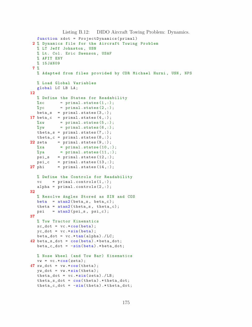
Listing B.12: DIDO Aircraft Towing Problem: Dynamics.function xdot = ProjectDynamics(primal)

2 % Dynamics file for the Aircraft Towing Problem

% LT Jeff Johnston , USN

% Lt. Col. Eric Swenson , USAF

% AFIT ENY

% 15JAN09

7 %

% Adapted from files provided by CDR Michael Hurni , USN , NPS

% Load Global Variables

global LC LB LA;

12

% Define the States for Readability

%xc = primal.states (1,:);

%yc = primal.states (2,:);

beta_s = primal.states (3,:);

17 beta_c = primal.states (4,:);

%xw = primal.states (5,:);

%yw = primal.states (6,:);

theta_s = primal.states (7,:);

theta_c = primal.states (8,:);

22 zeta = primal.states (9,:);

%xa = primal.statse (10 ,:);

%ya = primal.states (11 ,:);

psi_s = primal.states (12 ,:);

psi_c = primal.states (13 ,:);

27 phi = primal.states (14 ,:);

% Define the Controls for Readability

vc = primal.controls(1,:);

alpha = primal.controls(2,:);

32

% Resolve Angles Stored as SIN and COS

beta = atan2(beta_s, beta_c);

theta = atan2(theta_s , theta_c);

psi = atan2(psi_s , psi_c);

37

% Tow Tractor Kinematics

xc_dot = vc.*cos(beta);

yc_dot = vc.*sin(beta);

beta_dot = vc.*tan(alpha)./LC;

42 beta_s_dot = cos(beta).* beta_dot;

beta_c_dot = -sin(beta).*beta_dot;

% Nose Wheel (and Tow Bar) Kinematics

vw = vc.*cos(zeta);

47 xw_dot = vw.*cos(theta);

yw_dot = vw.*sin(theta);

theta_dot = vc.*sin(zeta)./LB;

theta_s_dot = cos(theta).* theta_dot;

theta_c_dot = -sin(theta).* theta_dot;

175

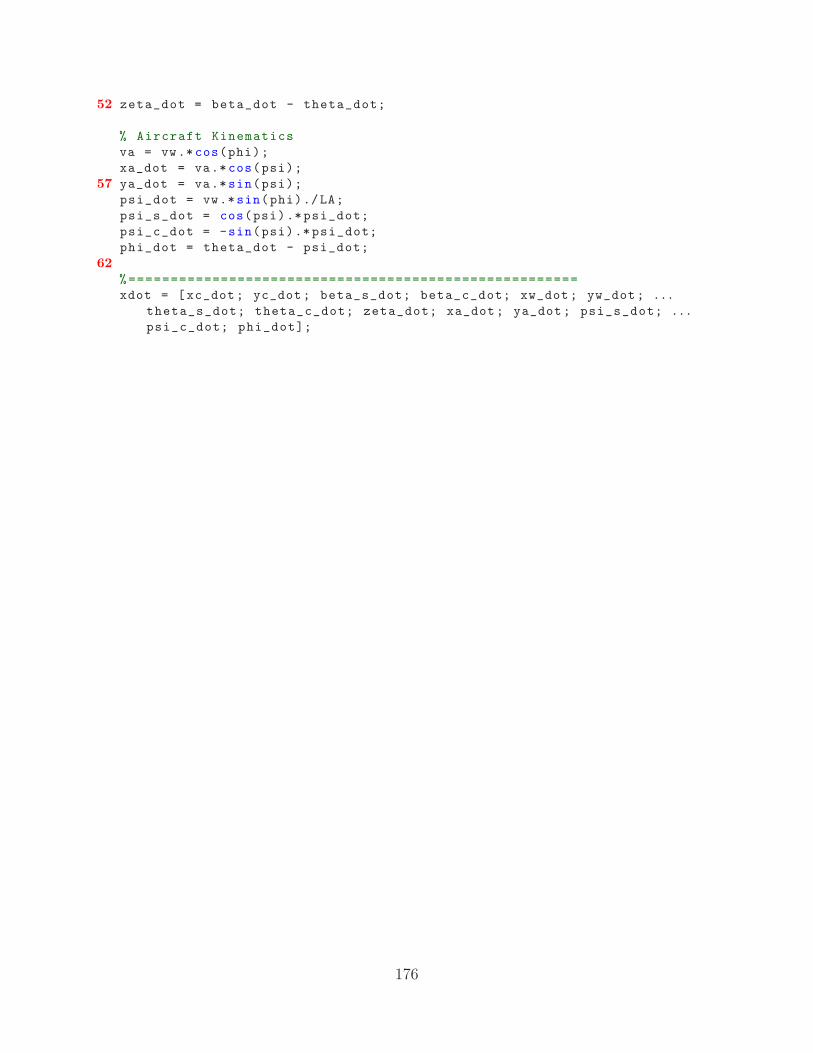
52 zeta_dot = beta_dot - theta_dot;

% Aircraft Kinematics

va = vw.*cos(phi);

xa_dot = va.*cos(psi);

57 ya_dot = va.*sin(psi);

psi_dot = vw.*sin(phi)./LA;

psi_s_dot = cos(psi).*psi_dot;

psi_c_dot = -sin(psi).* psi_dot;

phi_dot = theta_dot - psi_dot;

62

% ======================================================

xdot = [xc_dot; yc_dot; beta_s_dot; beta_c_dot; xw_dot; yw_dot; ...

theta_s_dot; theta_c_dot; zeta_dot; xa_dot; ya_dot; psi_s_dot; ...

psi_c_dot; phi_dot];

176

Listing B.13: DIDO Aircraft Towing Problem: Cost.1 function [EndpointCost , RunningCost] = ProjectCost(primal)

% Cost file for the Aircraft Towing Problem

% LT Jeff Johnston , USN

% Lt. Col. Eric Swenson , USAF

% AFIT ENY

6 % 15JAN09

%

% Adapted from files provided by CDR Michael Hurni , USN , NPS

% Define Cost Parameters

11 %tf = primal.nodes(end);

alpha = primal.controls(2,:);

% Calculate Cost

%min_steer = 1./(4*(alpha -pi/4)).^2;

16 min_steer = abs(alpha);

%EndpointCost = tf;

EndpointCost = 0;

RunningCost = min_steer;

177

B.2 C

Listing B.14: Source code of GPS logging software used for custom GPS recorders.

// Modified 08OCT08 by LT Jeff Johnston

// Originally written by Don Smith , AFIT Ctr , ANT Center

//

// Modified to write filenames in sequential order of creation

5

#include <stdio.h>

#include <stdlib.h>

//#include <conio.h>

#include <time.h>

10

int main(int argc , char** argv)

FILE* SerialDevice = NULL;

FILE* LogFile = NULL;

15 FILE* run_file;

char Buffer [2000];

char logfilename[256];

char date[20];

char command_exec[1024];

20 short int run = 0;

// Mark run file to continuously count # of times run

//NEED to add "run_file.txt" file to same directory as ...

main program

//WILL SEGFAULT IF YOU DON’T!!!

25 run_file = fopen("run_file.txt","r");

fscanf(run_file ,"%d",&run);

run=run+1;

fclose(run_file);

run_file = fopen("run_file.txt","w");

30 fprintf(run_file ,"%d",run);

fclose(run_file);

/* Open the serial device on COM2 readonly*/

SerialDevice = fopen("/dev/ttyS2", "r");

35 if (! SerialDevice)

fprintf(stderr, "Unable to open /dev/ttyS2 for ...

reading\n");

return -1;

40 /* Create and open the log file */

// sprintf(logfilename ,"/mnt/mmc/test21/data%d",date); //...

Old command uses random number

sprintf(logfilename ,"/mnt/mmc/gps_data/data%d",run); //...

Write file name with run number appended to end

LogFile = fopen(logfilename , "w"); //Opens file for ...

writing in ascii mode , use wb for binary

if (! LogFile)

178

45 fprintf(stderr, "Unable to create and open /mnt/...

mmc/gps_data/data%d for writing\n");

return -2;

/* In an infinite loop: read from serial device, write to ...

log file */

50 while (1)

//Use fread/fwrite if data is binary

//fread(Buffer, 1, 100, SerialDevice); //Read 100 ...

bin elements of size 1

//fwrite(Buffer, 1, 100, LogFile); //Write 100 bin...

elements of size 1

55

//Use fets/fputs if data is ASCII

if (fgets(Buffer , 2000, SerialDevice) == NULL)

fprintf(stderr , "Error or end of file ...

detected\n");

return -3;

60

if (fputs(Buffer , LogFile) == EOF)

fprintf(stderr , "Error writing data to /...

mnt/mmc/gps_data/data\n");

return -4;

65

/* Execution never reaches here but it makes the compiler ...

happy */

fclose(LogFile);

return 0;

70

179

Appendix C. Data Disc

A disc containing the data collected in the tests described in Chapter III was

created for distribution with this thesis document. The files and folders it

contains are described here.

The folder gps data contains a dated folder for each section of the test with re-

sults presented in Chapter IV. The folders 21OCT08, 22OCT08, and 23OCT08 con-

tain data collected at AFIT, while 20NOV08 contains data collected at NAS Oceana.

Each folder contains a subfolder exports which holds the carrier-phase differential so-

lutions generated by NovAtel Waypoint GrafNavTM. Each solution file is named with

the measurement device used and contains a description of the contents. They are

ASCII encoded with DOS end of line characters. Each dated folder also contains a

compressed binary file with the raw measurement data from each device stored as

raw data.tar.gz. These gzipped tarballs can be extracted using the GNU tar 1 and

gzip2 utilities, available for virtually any operating system. The 20NOV08 folder also

contains MATLABr script files used to generate the results of the data collection.

The path planning folder provides the DIDO Aircraft Towing Problem files used

to compute the path presented in Figure 4.24 on page 117 as well as the script

draw DIDO soln.m to create an animation of the resulting motion.

The final folder, scripts, contains MATLABr functions and data objects used to

generate both the results of data collection and the path planning plots.

1http://www.gnu.org/software/tar/2http://www.gzip.org/

180

Bibliography

1. Arya, Sunil, David M. Mount, Nathan S. Netanyahu, Ruth Silverman, andAngela Y. Wu. “An Optimal Algorithm for Approximate Nearest NeighborSearching in Fixed Dimensions”. J.ACM, 45(6):891–923, 1998. URL http:

//doi.acm.org/10.1145/293347.293348.

2. Bolzern, P., R. M. DeSantis, and A. Locatelli. “An Input-Output LinearizationApproach to the Control of an n-Body Articulated Vehicle”. Journal of DynamicSystems, Measurement, and Control, 123(3):309–316, 2001. URL http://link.

aip.org/link/?JDS/123/309/1;10.1115/1.1387010.

3. Bolzern, P., R. M. DeSantis, A. Locatelli, and D. Masciocchi. “Path-tracking forArticulated Vehicles with Off-axle Hitching”. Control Systems Technology, IEEETransactions on, 6(4):515–523, 1998.

4. Cobb, H. Stewart. GPS Pseudolites: Theory, Design, and Applications. Ph.D.thesis, Stanford University, 1997. URL http://waas.stanford.edu/~wwu/

papers/gps/PDF/Thesis/StewartCobbThesis97.pdf.

5. Commander, Naval Air Forces (CNAF). “The Naval Aviation Maintenance Pro-gram (NAMP)”, 30 Jun 2008. COMNAVAIRFORINST 4790.2A.

6. Commander, Naval Air Systems Command. “CV Flight/Hangar Deck NATOPSManual”, 2005. NAVAIR 00-80T-120.

7. Department of Defense (DoD). “Unmanned Systems Roadmap 2007-2032”, 2007.

8. Department of Defense (DoD). “Accident Investigation, Reporting, and RecordKeeping”, 2008. DODI 6055.07.

9. Department of the Navy (DON). “Naval Aviation Safety Program”, 2007. OP-NAVINST 3750.6R.

10. Dogan, A. “Probabilistic Approach in Path Planning for UAVs”. IntelligentControl. 2003 IEEE International Symposium on, 608–613, 2003.

11. Fox, Richard and Michael L. Nelson. “A Generic Path Planning Strategy for Au-tonomous Vehicles”. URL http://citeseerx.ist.psu.edu/viewdoc/summary?

doi=10.1.1.38.250. Unpublished.

12. Friedman, J. H., F. Baskett, and L. J. Shustek. “An Algorithm for Finding NearestNeighbors”. Computers, IEEE Transactions on, C-24(10):1000–1006, Oct. 1975.

13. Giardina, Thomas J. An Interactive Graphics Approach to the Flight Deck Han-dling Problem. Master’s thesis, Naval Postgraduate School, 1974.

14. Gong, Qi, Wei Kang, and I. M. Ross. “A Pseudospectral Method for the Opti-mal Control of Constrained Feedback Linearizable Systems”. Automatic Control,IEEE Transactions on, 51(7):1115–1129, 2006.

181

15. GPS NAVSTAR JPO. NAVSTAR GPS Space Segment / Navigation User Inter-faces. Technical report, 1999.

16. Grisso, Robert, Richard Oderwald, Mark Alley, and Conrad Heatwole. “Preci-sion Farming Tools: Global Positioning System (GPS)”. Virginia CooperativeExtension, 442(503), 2003. URL http://www.ext.vt.edu/pubs/bse/442-503/

442-503.pdf.

17. gumstix. “gumstix.com - way small computing”, 2008.

18. Ho, C. M., A. T. Mannucci, U. J. Lindqwister, and X. Q. Pi. “Global IonosphericPerturbations Monitored by the Worldwide GPS Network”, 1996. URL http:

//trs-new.jpl.nasa.gov/dspace/handle/2014/25455.

19. Hsu, David, Robert Kindel, Jean-Claude Latombe, and Stephen Rock. “Random-ized Kinodynamic Motion Planning with Moving Obstacles”. The InternationalJournal of Robotics Research, 21(3):233–255, 2002.

20. Hurni, Michael A., Pooya Sekhavat, and I. Michael Ross. “Autonomous Trajec-tory Planning Using Real-Time Information Updates”. AIAA Guidance, Nav-igation and Control Conference and Exhibit. Honolulu, HI, 18-21 August 2008.AIAA 2008-6305.

21. Hurni, Michael A., Pooya Sekhavat, and I. Michael Ross. “An Algorithm forAutonomous Optimal Control Trajectory Planning in Real-Time”. Proceedingsof the 19th AAS/AIAA Space Flight Mechanics Meeting. Savannah, GA, 9-12February 2009.

22. Hurni, Michael A., Pooya Sekhavat, and I. Michael Ross. “An Info-Centric Tra-jectory Planner for Unmanned Ground Vehicles”. International Conference onthe Dynamics of Information Systems. Gainesville, FL, 28-30 January 2009.

23. Jackson, Paul. Jane’s All the World’s Aircraft, volume 2001-2002. Sampson LowMarston and Co. London, 2001. ISBN 0 7106 2307 0. URL http://online.

janes.com/.

24. Johnson, Alan K. and Kriston P. Woolley. A Simulation of a Computer Graphics-Aided Aircraft Handling System. Master’s thesis, Naval Postgraduate School,1975.

25. King, R. S. Systems Definition Study of Carrier Aircraft Deck Operations ControlSystem (CADOCS). Technical Report NAEL-ENG-7453, Naval Air EngineeringCenter, 21 Apr 1967. AD877803.

26. Krozel, J. and D. Andrisani II. “Intelligent Epsilon-Optimal Path Predictionfor Vehicular Travel”. Systems, Man and Cybernetics, IEEE Transactions on,25(2):345–353, Feb 1995.

27. Larsson, U., C. Zell, K. Hyyppa, and A. Wernersson. “Navigating an ArticulatedVehicle and Reversing with a Trailer”. Robotics and Automation, 1994. Proceed-

182

ings., 1994 IEEE International Conference on, (on robust state estimation):2398–2404 vol.3, 1994.

28. Lee, T. H., H. K. Lam, F. H. F. Leung, and P. K. S. Tam. “A Fast Path Planning-and-Tracking Control for Wheeled Mobile Robots”. Robotics and Automation,2001.Proceedings 2001 ICRA.IEEE International Conference on, 2:1736–1741,2001.

29. Lewis, L. R., I. M. Ross, and Qi Gong. “Pseudospectral Motion Planning Tech-niques for Autonomous Obstacle Avoidance”. Decision and Control, 2007 46thIEEE Conference on, 5997–6002, 2007.

30. Lewis, Laird-Philip Ryan. Rapid Motion Planning and Autonomous ObstacleAvoidance for Unmanned Vehicles. Master’s thesis, Naval Postgraduate School,2006.

31. Mahr, Randolph, Bruce Chiodi, and Mike Jones. “Aviation Data Managementand Control Systems (ADMACS)”, 2008. Presentation, Naval Air Systems Com-mand.

32. Microsoft. “Tampa Authorities deploy latest technology for Super Bowl Secu-rity”, 2009. URL http://www.microsoft.com/industry/government/news/e_

sponder_super_bowl.mspx.

33. Misra, Pratap and Per Enge. Global Position System: Signals, Measurements, andPerformance. Ganga-Jamuna Press, Lincoln, MA, 2006. ISBN 0-9709544-1-7.

34. Naval Air Systems Command (NAVAIR). Unmanned Combat Air System CVDemonstration (UCAS-D) Performance Specification. Technical Report NA-4150-UCAS-1003, 2007.

35. Naval Safety Center. “Flight Deck Awareness Guide”, 2003. URL http://www.

safetycenter.navy.mil/aviation/downloads/index.asp.

36. Ng, Teck Chew, J. I. Guzman, and M. D. Adams. “Autonomous Vehicle-followingSystems : A Virtual Trailer Link Model”. Intelligent Robots and Systems, 2005.(IROS 2005). 2005 IEEE/RSJ International Conference on, 3057–3062, 2005.

37. Northrop Grumman Corporation, Newport News. “ACOMS Spot Sheet Lite”,2003.

38. Novatel Inc. “OEMV Family Firmware Reference Manual”, 2008.

39. Novatel Inc. “OEMV Family Installation and Operation User Manual”, 2008.

40. NovAtel Waypoint Products Group. “Waypoint GrafNav/GrafNet”, 2007. URLhttp://www.novatel.com/products/waypoint_grafnav.htm.

41. Park, Myoungkuk, Woojin Chung, Munsang Kim, and Jaebok Song. “Controlof a Mobile Robot with Passive Multiple Trailers”. Robotics and Automation,2004. Proceedings. ICRA ’04. 2004 IEEE International Conference on, 5:4369–4374 Vol.5, 2004.

183

42. Rainwater, C. W. CADOCS Subsystems; Parameter Definition. Technical ReportNAEC-ENG-7536, Naval Air Engineering Center, 24 Mar 1967. AD852865.

43. Rainwater, C. W. Exploratory Study of an Automated Carrier Aircraft DeckOperations Control System. Technical Report NAEL-ENG-7375, Naval Air Engi-neering Center, 21 Oct 1966. AD819612.

44. Rainwater, C. W. and G. R. Ruddick. CADOCS Subsystem Requirements Studies.Technical Report NAEC-ENG-7466, Naval Air Engineering Center, 26 Jan 1968.AD905456.

45. Rider, Timothy L. “Blue Force Tracking to Expand Across Force”. Army Acqui-sition, Logistics, and Technology, (September-October):2, 2004.

46. Ross, I. M. User’s Manual for DIDO: A MATLAB Application Package forSolving Optimal Control Problems. Elissar, Monterey, CA, 2007. Document TR705.

47. Segall, Paul and James Davis. “GPS APPLICATIONS FOR GEODYNAMICSAND EARTHQUAKE STUDIES”. Annual Review of Earth and Planetary Sci-ences, 25:301, 1997.

48. Stentz, A. “Optimal and Efficient Path Planning for Partially-known Environ-ments”. Robotics and Automation, 1994. Proceedings., 1994 IEEE InternationalConference on, 3310–3317 vol.4, 1994.

49. Tiboni, Frank and Matthew French. “Blue Force Tracking Gains Ground”. FederalComputer Week, 2008(12/15), 2004. URL http://www.fcw.com/print/10_7/

news/82385-1.html.

50. Tiron, Roxana. “Army’s Blue-Force Tracking Technology Was a Tough Sell”.National Defense, (December), 2003.

51. Tolman, Brian, R. Benjamin Harris, Tom Gaussiran, David Munton, Jon Lit-tle, Richard Mach, Scot Nelsen, and Brent Renfro. “The GPS Toolkit: OpenSource GPS Software”. Proceedings of the 16th International Technical Meetingof the Satellite Division of the Institute of Navigation. Long Beach, California,September 2004.

52. United States Coast Guard. “CONUS GPS PDOP Chart - USCG NavigationCenter”, 2009. URL http://www.navcen.uscg.gov/gps/pdop.htm.

53. Vallado, David A. Fundamentals of Astrodynamics and Applications. KluwerAcademic Publishers, Dordrecht, Boston, London, 2001. ISBN 1-881883-12-4.

54. Venetsky, Larry, Mark Husni, and Mark Yager. Gesture Recognition for UCAV-N Flight Deck Operations. Technical Report ADA422629, Naval Air SystemsCommand, 23 Jan 2003.

55. Wilt, Jim and Valerie Bjorn. “Noise and Advanced Hearing Protection”,2006. URL http://www-nehc.med.navy.mil/downloads/occmed/hctoolbox/

Toolbox_files/NAVAIR%20Advanced%20Hearing%20Protection.ppt.

184

56. Yang, Guang and V. Kapila. “Optimal Path Planning for Unmanned Air Ve-hicles with Kinematic and Tactical Constraints”. Decision and Control, 2002,Proceedings of the 41st IEEE Conference on, 2:1301–1306 vol.2, 2002.

185

Vita

Lieutenant Jeffrey S. Johnston graduated from Boonsboro High School in Boons-

boro, Maryland. He entered undergraduate studies at the University of Maryland in

College Park, Maryland where he graduated with a Bachelor of Science degree in

Aerospace Engineering in May 2003. In October 2001 he enlisted in the United

States Navy through the Baccalaureate Degree Completion Program and received his

commission through Officer Candidate School, NAS Pensacola, Florida in 2004.

Following Aviation Maintenance Duty Officer training he was assigned to Strike

Fighter Squadron THREE FOUR, the Blue Blasters, an FA-18C Hornet squadron

stationed at NAS Oceana, Virginia Beach, VA where he served as Material Control

Officer, Aircraft Division Officer, and Assistant Maintenance Officer. From June to

December 2004 he was deployed with his squadron onboard USS John F. Kennedy

(CV 67) and participated in Operation Iraqi Freedom. He deployed with his squadron

again from March to August 2006 onboard USS Abraham Lincoln (CVN 72) to the

Western Pacific.

In August 2007 he entered the Graduate School of Engineering and Management

at the Air Force Institute of Technology. Upon graduation he will be assigned to Space

and Naval Warfare Systems Command (SPAWAR), Space Field Activity, Chantilly,

VA.

Permanent address: 2950 Hobson WayAir Force Institute of TechnologyWright-Patterson AFB, OH 45433

186

NONPRINT FORM

1. Type of Product:

2. Operating System/Version:

3. New Product or Replacement:

4. Type of File:

5. Language/Utility Program: 6. # of Files/# of Products:

7. Character Set:

8. Disk Capacity:

9. Compatibility:

10. Disk Size:

11. Title: 12. Performing Organization:

13. Performing Report #:

14. Contract #:

15. Program Element #:

16. Sponsor/Monitor:

17. Sponsor/Monitor # Acronym:

19. Project #:

18. Sponsor/Monitor #:

20. Task #:

21. Work Unit #:

22. Date:

23. Classification of Product:

24. Security Classification Authority:

25. Declassification/Downgrade Schedule:

26. Distribution/Availability: DTIC FORM 530 JUN 94 Security Classification of this Page:

NONPRINT FORM

27. Abstract: 28. Classification of Abstract:

29. Limitation of Abstract:

30. Subject Terms:

30a. Classification of Subject Terms:

31. Required Peripherals: 32. # of Physical Records:

33. # of Logical Records:

34. # of Tracks:

35. Record Type:

36. Color:

37. Recording System:

38. Recording Density:

39. Parity:

40. Playtime:

41. Playback Speed:

42. Video:

43. Text:

44. Still Photos:

45. Audio:

46. Other: 47. Documentation/Supplemental Information: 48. Point of Contact and Telephone Number: DTIC FORM 530 JUN 94 Security Classification of this Page:

REPORT DOCUMENTATION PAGE Form Approved OMB No. 0704–0188

The public reporting burden for this collection of information is estimated to average 1 hour per response, including the time for reviewing instructions, searching existing data sources, gathering and maintaining the data needed, and completing and reviewing the collection of information. Send comments regarding this burden estimate or any other aspect of this collection of information, including suggestions for reducing this burden to Department of Defense, Washington Headquarters Services, Directorate for Information Operations and Reports (0704–0188), 1215 Jefferson Davis Highway, Suite 1204, Arlington, VA 22202–4302. Respondents should be aware that notwithstanding any other provision of law, no person shall be subject to any penalty for failing to comply with a collection of information if it does not display a currently valid OMB control number. PLEASE DO NOT RETURN YOUR FORM TO THE ABOVE ADDRESS. 1. REPORT DATE (DD–MM–YYYY) 26-03-2009

2. REPORT TYPE Master’s Thesis

3. DATES COVERED (From — To) September 2007 – March 2009

4. TITLE AND SUBTITLE A Feasibility Study of A Persistent MonitoringSystem For The Flight Deck of U.S. NavyAircraft Carriers.

5a. CONTRACT NUMBER

5b. GRANT NUMBER

5c. PROGRAM ELEMENT NUMBER

6. AUTHOR(S) LT Jeffrey S. Johnston, USN

5d. PROJECT NUMBER 5e. TASK NUMBER

5f. WORK UNIT NUMBER

7. PERFORMING ORGANIZATION NAME(S) AND ADDRESS(ES) Air Force Institute of Technology Graduate School of Engineering and Management (AFIT/ENY) 2950 Hobson Way WPAFB OH 45433-7765

8. PERFORMING ORGANIZATION REPORT NUMBER AFIT/GAE/ENY/09-M12

9. SPONSORING / MONITORING AGENCY NAME(S) AND ADDRESS(ES) Intentionally left blank

10. SPONSOR/MONITOR’S ACRONYM(S)

11. SPONSOR/MONITOR’S REPORT NUMBER(S)

12. DISTRIBUTION / AVAILABILITY STATEMENT APPROVED FOR PUBLIC RELEASE; DISTRIBUTION UNLIMITED

13. SUPPLEMENTARY NOTES

14. ABSTRACT This research analyzes the use of modern Real Time Locating Systems (RTLS), such as the Global Positioning System (GPS), to improve the safety of aircraft, equipment, and personnel onboard a United States Navy (USN) aircraft carrier. The results of a detailed analysis of USN safety records since 1980 show that mishaps which could potentially be prevented by a persistent monitoring system result in the death of a sailor nearly every other year and account for at least $92,486,469, or 5.55% of the total cost of all flight deck and hangar bay related mishaps. A system to continually monitor flight deck operations is proposed with four successive levels of increasing capability. A study of past and present work in the area of aircraft carrier flight deck operations is performed. This research conducted a study of the movements of USN personnel and an FA-18C aircraft being towed at NAS Oceana, VA. Using two precision GPS recorders mounted on the aircraft wingtips, the position and orientation of the aircraft, in two-dimensions, are calculated and the errors in this solution are explored. The distance between personnel and the aircraft is calculated in the nearest neighbor sense. Pseudospectral motion planning techniques are presented to provide route prediction for aircraft, support equipment, and personnel. Concepts for system components, such as aircraft and personnel receivers, are described. Methods to recognize and communicate the presence of hazardous situations are discussed. The end result of this research is the identification of performance requirements, limitations, and definition of areas of further research for the development of a flight deck persistent monitoring system with the capability to warn of hazardous situations, ease the incorporation of UAVs, and reduce the risk of death or injury faced by sailors on the flight deck. 15. SUBJECT TERMS AIRCRAFT CARRIERS, GLOBAL POSITIONING SYSTEM, MOTION, FLIGHT DECKS, KINEMATICS, PATH PLANNING, AVIATION SAFETY 16. SECURITY CLASSIFICATION OF: 17. LIMITATION

OF ABSTRACT UU

18. NUMBER OF PAGES 205

19a. NAME OF RESPONSIBLE PERSON Lt Col Eric D. Swenson

a. REPORT U

b. ABSTRACT U

c. THIS PAGE U

19b. TELEPHONE NUMBER (Include Area Code) (937) 785-3636 x7479 eric.swenson@afit.edu

Standard Form 298 (Rev. 8–98) Prescribed by ANSI Std. Z39.18