A Fast Branch-and-Prune Algorithm

for the Position Analysis of

Spherical Mechanisms

Arya Shabani, Soheil Sarabandi, Josep M. Porta, and Federico Thomas

Institut de Robotica i Informatica industrial, CSIC-UPC,Llorens Artigas 4-6, 080028 Barcelona, Spain,

{ashabani, ssarabandi, porta, fthomas}@iri.upc.edu.

Abstract. Different branch-and-prune schemes can be found in the lit-erature for numerically solving the position analysis of spherical mecha-nisms. For the prune operation, they all rely on the propagation of motionintervals. They differ in the way the problem is algebraically formulated.This paper exploits the fact that spherical kinematic loop equations canbe formulated as sets of 3 multi-affine polynomials. Multi-affinity has animportant impact on how the propagation of motion intervals can beperformed because a multi-affine polynomial is uniquely determined byits values at the vertices of a closed hyperbox defined in its domain.

Keywords: multi-affine polynomials, parallel spherical robots, forwardkinematics, position analysis, branch-and-prune algorithms

1 Introduction

Solving systems of geometric constraints is a fundamental topic in Computa-tional Kinematics, Computer Graphics, and Computational Chemistry. In Com-putational Kinematics, it is commonly referenced to as position analysis or dis-placement analysis which includes the inverse (forward) kinematics of serial (par-allel) robots.

The solution to position analysis problems is usually preferred to be in closed-form. That is, the solution is given as the roots of a closure polynomial of the low-est possible degree in a single variable (sometime called characteristic equation

of the mechanism). The most straightforward approach to obtain these polyno-mials consists in applying a series of variable eliminations to a set of independentkinematic loop equations. Nevertheless, to make this process practical, it is usu-ally needed to simplify the formulation by exploiting the particularities of eachproblem instance. As a result, obtaining the 16-degree closure polynomial of ageneral 6R robot [1] is quite different from obtaining the 40-degree closure poly-nomial of a general Gough-Stewart parallel platform [2]. Automating the processto obtain these polynomials for any case in a reasonable amount of time seemsimpossible at the moment. Nevertheless, if instead of a set of kinematic loopequations, a distance-based formulation is used, a higher lever of generality and

2 A. Shabani et al.

uniformity has recently been obtained thus opening an avenue for an automaticanalysis without ad hoc considerations (see [3] for a step in this direction).

Alternatively to obtain a closure polynomial, it is possible to directly computethe solutions of the system of loop equations by using numerical approaches suchas those based on numerical continuation or interval methods (see, for example,[4] and [5], respectively). These numerical approaches are the only alternative tolarge problems like those arising in mechanism synthesis.

The closed-form position analysis of spherical mechanisms (mechanisms con-structed by connecting links with hinged joints such that the axes of each hingepasses through the same point) has received the attention of different authors.For example, the methods presented by Wampler in [6] and by Bai et al. in [7]can be applied to obtain closure polynomials for spherical mechanisms with upto three and to two independent kinematic loops, respectively. Numerical ap-proaches has also been tested. Bombın et al. reformulated the kinematic loopequations in terms of Bernstein polynomials [8, 9]. This permited to formulatethe problem in terms of control points, which could be recalculated for arbi-trary ranges using a simple subdivision procedure. Celaya presented an inge-nious method to exactly propagate intervals of motion in a spherical kinematicloop [10]. The iterative application of this method to all the kinematic loopsdescribing the problem at hand permitted to converge to all the solutions.

The work of Bombın introduced an important concept in position analysis:that of control points. Specifying curves and surfaces in terms of control points isone of the major techniques used in geometric design [11]. The idea is simple: thevalues of a polynomial function in a given domain (usually an othotope) lie insidethe region determined by the convex hull of a set of control points whose numberdepend on the degree of the polynomial. Obtaining these control points requiresexpressing the polynomials in Bernstein base. Nevertheless, if the polynomialsare multi-linear or even multi-affine, this operation is trivial because the controlpoints are obtained by simply evaluating the polynomial at the corners of theorthotope defining the domain.

Although any polynomial can be easily transformed into a system of multi-affine polynomials by introducing new variables and more equations (as it isdone, for example, in [12]), increasing the number of equations is not, in general,a good idea. Fortunately, we will show in this paper how the proper formulationof kinematic loop equations in spherical mechanisms directly leads to a minimalset of multi-affine polynomials. As a consequence, a simple and yet very effectivebranch-and-prune algorithm is derived to obtain the roots of these systems ofequations.

This paper is organized as follow. The next section describes how to obtainan multi-affine formulation for the kinematic loop equations in spherical mecha-nisms using quaternions. Section 3 deals with the numerical problem introducedby the Weierstrass substitution, implicit in the proposed formulation, and how toavoid it. The branch-and-prune algorithm is described in Section 4. The behaviorof this algorithm is analyzed in Section 5 for three problems of increasing com-plexity. Finally, Section 6 summarizes the points and gives some prospects for

A Fast Branch-and-Prune Algorithm 3

feature research such as the generalization of the presented approach to spatialmechanisms.

2 Kinematic loop equations in spherical mechanisms

An spherical kinematic loop equation can always be formulated in terms ofproducts of unit quaternions

q1 · q2 . . . qr = 1, (1)

where each quaternion has the form

qi =1

√

t2i + 1[1 + ti(pixi+ piyj + pizk)] , (2)

where pi = (pix piy piz) is a unit vector representing the rotation axis and ti =

tan(

φi

2

)

, φi being the rotated angle about it. The angle φi can be constant or

variable.The expansion of equation (1) leads, after clearing denominators, to the fol-

lowing four scalar equations

f0(t1, . . . , tn) =√

(t21 + 1) · · · (t2n + 1),

fj(t1, . . . , tn) = 0, j = 1, 2, 3,

where in the parentheses only appear the variable ti, i = 1, . . . , n which have beenrenumbered, that is, n ≤ r. These four equations are not independent becausethey correspond to the components of a unit quaternion. While fj , j = 1, 2, 3,are affine polynomials in each variable, f0, after clearing the radical, leads to aquadratic polynomial. For obvious simplicity reasons, in what follows, we willtake fj , j = 1, 2, 3, as the set of three independent equations. Therefore, if ourproblem can be described in terms of n independent loop equations, we will havea set of 3n multi-affine polynomial equations.

A word of caution should be added here. Sometimes, in an abuse of language,a system of equations like the one given by fj , j = 1, 2, 3, is called multi-linear.Strictly speaking, it is multi-affine. Indeed, fj can be expressed as a function ofti as fj = ajti + bj which is not linear in ti, but affine.

Multi-affine polynomials have two interesting properties which are very usefulfor our purposes. If we have an affine polynomial function whose domain is anorthotope, then

– the value of the function in any point inside the domain defined by theorthotope is inside the convex hull of the points resulting from evaluatingthe function at the corners of the orthotope [13].

– the polynomial function is completely determined by the values of the func-tion at the corners of the orthotope. The value of the function in any otherpoint can be obtained by a simple interpolation procedure [14].

These two properties are exploited in Section 4.

4 A. Shabani et al.

3 Numerical issues derived from the Weierstrass

substitution

t = 0

t = 0.5

t = 1

t = 2

t = 3

t = −1

∞

Fig. 1. The Weierstrass substitutionmaps the interval [−π, π] onto the in-terval [−1, 1]. Numerical problems ariseas we approach π because it is mappedonto ∞.

In above formulation, the variable ti isrelated to the angle variable φi thought

the relationship ti = tan(

φi

2

)

, that is,

the tangent half-angle substitution (alsoknown as the Weierstrass substitution).From the geometric point of view, thissubstitution can be seen as the stereo-graphic projection of the unit circle, fromx = −1, to the line y = 0 (see Fig. 1).Thus, if φi = π, ti is infinity. Then, if amechanism has a solution near π, numer-ical problems occur. Moreover, if we wantto apply a branch-and-prune method toobtain the solutions of our system of equa-tions, it is not a good decision to startwith a domain ranging from −∞ to +∞in all variables. One possible solution tothis situation is to split the problem intwo: one for φi ∈ [−π/2, π/2], and an-other one for φ′

i ∈ [−π/2, π/2], whereφ′

i = φi + π. The second problem justconsists in shifting the origin of the ro-tation about pi π radians. This can beaccomplished by including a constant ro-tation prior to the variable rotation aboutthe same axis. For example, if in the loopequation q1 · q2 . . . qr = 1, we want toshift the origin of the rotation about pi,

1 ≤ i ≤ r, π radians, we just have to substitute qi by (ipx + jpy + kpz)qi.This operation has to be done for all variables. In other words, if our problemhas r variables, we will decompose it into 2r equivalent problems in the do-main [−1, 1]1 × [−1, 1]2 × . . . [−1, 1]r. Having this domain for all problems hasan important extra advantage: if the values of the functions are obtained by in-terpolation from the values of the function at the corners of the initial domain,this is simplified because all coordinates are −1 or 1.

4 Solving multi-affine polynomial systems

Let us define the equationF(x) = 0, (3)

where F = (f1(x), . . . , fm(x)), and each function fi is a multi-affine polynomialin the unknowns x1, . . . , xn.

A Fast Branch-and-Prune Algorithm 5

Next, we describe an algorithm able to isolate all solutions of (3) that liein the orthotope B ∈ R

n defined as the Cartesian product B = [xl1, x

u1 ] × · · · ×

[xln, x

un].

4.1 A branch-and-prune scheme

Generally speaking, the algorithm isolates the solutions by iterating two oper-ations, box reduction and box bisection, using the following branch-and-prunescheme. Using box reduction, portions of B containing no solution are cut offby narrowing some of its defining intervals. This process is iterated until either(1) the box is reduced to an empty set, in which case it contains no solution,or (2) the box is “sufficiently” small, in which case it is considered a solutionbox, or (3) the box cannot be “significantly” reduced, in which case it is splitinto two sub-boxes via box bisection. If the latter occurs, the whole process isrepeated for the newly created sub-boxes, and for the sub-boxes recursively cre-ated thereafter, until one ends up with a collection of boxes whose size is undera specified size threshold, as explained in detail below.

If there is only a finite number of solution points in B, this algorithm returnsa collection of small boxes containing them all. If, contrarily, the solution space isan algebraic variety of dimension one or higher, the algorithm returns a collectionof small boxes discretizing the portions of this variety contained in B. In all cases,the algorithm is complete, in the sense that every solution point will be containedin one of the returned boxes.

Let us now follow the box reduction and bisection operations in detail, tolater see how they fit into the algorithm.

4.2 Box reduction and box bisection

The box reduction operation is based on the following lemma, which is a directconsequence of Theorem 1.1 in [13]:

The point (x, f(x)) ∈ Rn+1, where f is a scalar multi-affine function

and x = (x1, . . . , xn) is a point lying in B = [xl1, x

u1 ] × · · · × [xl

n, xun], is

contained in the convex hull of the 2n points {(x, f(x)) | x ∈ {xl1, x

u1} ×

. . .× {xln, x

un}}.

In other words, the graph of f(x) corresponding to a box B necessarily lies insidethe convex hull of the 2n points of the form (x, f(x)), where x is a corner of B.

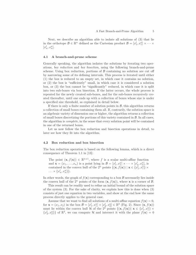
This result can be readily used to refine an initial bound of the solution spaceof the system (3). For the sake of clarity, we explain how this is done when (3)consists of just one equation in two variables, and show at the end how the sameprocess directly applies to the general case.

Assume that we want to find all solutions of a multi-affine equation f(x) = 0,for x = (x1, x2) in the box B = [xl

1, xu1 ]× [xl

2, xu2 ] ∈ R

2 (Fig. 2). Since (x, f(x))must lie within the convex hull H of the 22 points {(x, f(x))| x ∈ {xl

1, xu1} ×

{xl2, x

u2}} of R3, we can compute H and intersect it with the plane f(x) = 0

6 A. Shabani et al.

f(x1, x2) f(x1, x2)

f(x1, x2)

x2

x2x1

x1

xl

2xu

2xl

1xu

1

xl

2

xu

2 xu

1

xl

1

Fig. 2. If f(x1, x2) is multi-affine, due to the convex hull property, the image of thepoints in the domain [xl

1, xu

1 ]× [xl

2, xu

2 ] (shown in red) necessarily lies inside the showntetrahedron. The vertices of this tetrahedron (shown in green) are obtained by evalu-ating f in the corners of the domain. Then, from the projections of this tetrahedrononto the coordinate planes (shown in blue), the initial ranges for the variables can bereduced to the regions where these projections intersect the coordinate axes.

to obtain a polygon whose smallest enclosing box gives a better bound for thesolutions. Since the explicit computation of H and its intersection with f(x) = 0are inefficient operations when f depends on a high number of variables, we willadopt the following variation of this technique: we simply project the hull Honto each coordinate plane, as depicted in Fig. 2 (top), and intersect each ofthe resulting trapezoids with the f(x) = 0 line, as shown in Fig. 2 (bottom).Clearly, from the initial range of a variable we can prune those points for whichthe trapezoid does not intersect the f(x) = 0 line. Thus, these segment-trapezoidclippings usually reduce the ranges of some variables giving a smaller box thatstill bounds the root locations (see the black rectangle in Fig. 2). The experimentsshow that, although this strategy produces less pruning than the convex hull-plane clipping, it results advantageous due to the lower cost of its operations.

A Fast Branch-and-Prune Algorithm 7

x y

z

θ1

θ2

θ3

P4

P5

P6

P7

P8

P9

P1

P2

P3

Oα1

α2

α3

1

P1P1

P2P3

P4

P5

P6

P7

P8

P9

P10

P12

Fig. 3. The three test cases used to validate the branch-and-prune algorithm presentedin this paper. Left: A spherical wrist. Center: 3-RRR parallel spherical manipulator.Right: A four loop spherical mechanism.

Note that exactly the same pruning strategy can be applied to a multi-affineequation in n variables, with n > 2, because the convex hull of the (then) involved2n points will also yield a trapezoidal polygon when projected to a plane definedby the xi and f(x) axes, for i = 1, . . . , n. Finally, if we have more than oneequation in the system, the process can be clearly iterated for all equations byapplying the pruning process of each equation onto the box produced by thepruning process of the preceding one.

The previous box reduction procedure is repeatedly applied on a same boxuntil one of the following conditions is met:

– The box gets empty. This happens when we are treating an equation f(x) = 0and a trapezoid does not intersect the corresponding coordinate axis. In anycase, we can stop the exploration in the current box.

– The reduction of the box volume between two consecutive iterations is belowa given threshold ρ. At this point, as the box cannot be significantly reduced,it is split into two sub-boxes via box bisection. This operation simply dividesthe longest variable range of the box into two halves. Box reduction andbisection are then recursively applied to the newly created sub-boxes.

– The longest side of the box is under a specified threshold σ. Here, the boxis considered a “solution box” since, if σ is sufficiently small, either this boxcontains a solution or is very close to one. Hence, it is added to the final listof boxes to be returned by the algorithm.

5 Examples

The described branch-and-prune algorithm has been implemented in C and eval-uated on three mechanisms of increasing complexity (see Fig. 3). The first oneis a simple spherical wrist whose inverse kinematics consists in solving a singlekinematic loop. The second is a 3-RRR [15] orienting robot whose forward kine-matics consists in solving two independent kinematic loops. The third one is aspherical mechanism with four independent kinematic loops [16].

8 A. Shabani et al.

Table 1. Summary of the results in the tree test cases. See the text for details.

l r p b be bs s t[ms]

1 3 8 1 0 1 1 32 6 64 241 107 14 2 54 12 2048 563 276 6 2 9

The inverse kinematics of the spherical wrist in Fig. 3(left) consists in obtain-

ing the values of ti = tan(

φi

2

)

, i = 1, 2, 3, which satisfy the following equation:

1√

(t21 + 1)(t22 + 1)(t23 + 1)(1 + t1k)(1 + t2i)(1 + t3k)q

−1o = 1, (4)

where q0 is the desired orientation for the end-effector. If we set q−10 = e0+e1i+

e2j+ e3k, we derive a set of three multi-affine equations which can be expressedin matrix form as:

e1 −e2 e0 −e2 e3 −e1 −e3 e0e2 e1 −e3 e1 e0 −e2 −e0 −e3e3 e0 e2 e0 −e1 −e3 e1 e2

1t1t2t3t1t2t1t3t2t3t1t2t3

= 0 (5)

The problem of solving the forward kinematics of the 3-RRR spherical par-allel manipulator shown in Fig. 3(center) consist in locating the triangle P7P8P9

with respect to the base P1P2P3 as a function of the motor angles θ1, θ2, and θ3.This mechanism has two independent kinematic loops, which, when formulatedin terms of quaternions as described in Section 2, give six multi-affine equationsin six unknowns.

Finally, the four-loop mechanism in Fig. 3(rigth) can be formulated, oncerepresented using quaternions, in terms of 12 multi-affine equations in 12 un-knowns.

Table 1 summarizes the performance of the algorithm described in Section 3with ρ = 0.99 and σ = 10−4. For each case, the table gives the number of loops(l), the number of variables (r), the number of initial boxes with all the variablesin the range [−1, 1] that can be defined (p = 2r), the number of processed boxesfor one of those initial search boxes (b), the number of empty boxes (be), thenumber of solution boxes (bs), the number of roots of the system (s), and theexecution time in milliseconds (t). The program is executed on a PC with anIntel Core 7 processor running at 4.2 GHz.

A Fast Branch-and-Prune Algorithm 9

6 Conclusion

We have presented an easy-to-implement branch-and-prune algorithm for solv-ing position analysis problems of spherical mechanisms. The simplicity of theproposed algorithm comes with two main disadvantages; namely:

– The use of one equation at a time leads to the so-called cluster problem,that is, each solution is obtained as a cluster of boxes instead of a singlebox containing it [17]. This is clear in Table 1 where, for the two-loop andfour-loop problems, the algorithm returns more solution boxes (bs) than theactual number of roots (s). All the solution boxes, though, are close to theactual solutions and the error (i.e., the norm of the residue of the equations)evaluated at the center of the solution boxes is below 10−3 in all cases. Thus,the clusters for each solution can be readily identified.

– The use of a single variable at a time makes the convergence to the roots belinear while other standard interval-based algorithms exhibit quadratic con-vergence [18]. Although our algorithm compares unfavorably in this respect,it should be beared in mind that we are actually facing a trade-off betweencost of each iteration and convergence rate.

Despite these drawbacks, the presented algorithm is remarkable for its sim-plicity, efficiency, and easy parallelization.

Finally, it is worth to mention that its extension to spatial mechanisms isperfectly feasible by approximating, for example, dual quaternions by doublequaternions ??. This point is currently concentrating our efforts.

References

1. M. Raghavan and B. Roth, “Inverse kinematics of the general 6R manipulator andrelated linkages,” ASME Journal of Mechanical Design, Vol. 115, pp. 502-508, 1993.

2. M.L.Husty, “An algorithm for solving the direct kinematics of general Stewart-Gough platforms,”’ Mechanism and Machine Theory, Vol. 31, No. 4, pp. 365-379,1996.

3. J.M. Porta and F. Thomas, “Yet another approach to the Gough-Stewart platformforward kinematics,” Proc. of the IEEE International Conference in Robotics and

Automation, Brisbane, Australia, 2018.4. C. Wampler, A. Morgan, and A. Sommese, “Numerical continuation methods for

solving polynomial systems arising in kinematics,” ASME Journal Mechanical De-

sign, Vol. 112, pp. 59-68, 1990.5. A. Castellet and F. Thomas, “An algorithm for the solution of inverse kinematics

problems based on an interval method,” Advances in Robot Kinematics, M. Hustyand J. Lenarcic (Eds.), pp. 393-403, Kluwer, 1998.

6. C.W. Wampler, “Displacement analysis of spherical mechanisms having three orfewer loops,” ASME Journal of Mechanical Design, Vol. 126, No. 1, pp. 93-100,2004.

7. S. Bai, M. R.Hansen, and J. Angeles, “A robust forward-displacement analysis ofspherical parallel robots,” Mechanism and Machine Theory, Vol. 44, No. 12, pp.2204-2216, 2009.

10 A. Shabani et al.

8. C. Bombın, L. Ros, and F. Thomas, “A concise Bezier clipping technique for solvinginverse kinematics problems,” Advances in Robot Kinematics, J. Lenarcic and M.Stanisic (Eds.), pp.53-61, Kluwer, 2000.

9. C. Bombın, L. Ros, and F. Thomas, “On the computation of the direct kinematics ofparallel spherical mechanisms using Bernstein polynomials,” Proc. IEEE Int. Conf.

on Robotics and Automation, Seoul, Korea, 2001.10. E. Celaya, “Interval propagation for solving parallel spherical mechanisms,” Ad-

vances in Robot Kinematics, J. Lenarcic and F. Thomas (Eds.), pp. 415-422,Springer, 2002.

11. J. Gallier, Curves and Surfaces in Geometric Modeling: Theory And Algorithms,Morgan Kaufmann, 1999.

12. J.M. Porta, L. Ros, F. Thomas, and C. Torras, “A branch-and-prune solver fordistance constraints,” IEEE Transactions on Robotics, Vol. 21, No. 2, pp. 176-187,2005.

13. A. Rikun, A convex envelope formula for multilinear functions, Journal of Global

Optimization, Vol. 10, No. 4, pp.425-437, 1970.14. R. Wagner, “Multi-linear interpolation,” Web document available at:

http://rjwagner49.com/Mathematics/Interpolation.pdf, 2004.15. X. Kong and C.M. Gosselin, “Type synthesis of 3-DOF spherical parallel manipu-

lators based on Screw Theory,” ASME Journal Mechanical Design, Vol. 126, No. 1,pp. 101-108, 2004.

16. J. Borras, R. Di Gregorio, “Direct position analysis of a large family of sphericaland planar parallel manipulators with four loops,” Second International Workshop

on Fundamental Issues and Future Research Directions for Parallel Mechanisms and

Manipulators, pp. 19-29, 2008.17. A. Morgan and V. Shapiro, “Box-bisection for solving second-degree systems and

the problem of clustering,” ACM Transactions on Mathematical Software, Vol. 13,No. 2, pp. 152-167, 1987.

18. E. Sherbrooke and N. Patrikalakis, “Computation of the solutions of nonlinearpolynomial systems,” Computer Aided Geometric Design, Vol. 10, No. 5, pp. 379-405, 1993.

19. F. Thomas, “Approaching dual quaternions from matrix algebra,” IEEE Transac-

tions on Robotics, Vol. 30, No. 5, pp. 1037-1048, 2014.