A exible hyperspectral simulation tool for complex ...cnspci/references/goodenough2006.pdf · Adam...

A flexible hyperspectral simulation tool for complex littoralenvironments

Adam Goodenougha, Rolando Raquenoa, Michael Bellandia, Scott Browna, and John Schotta

aDigital Imaging and Remote Sensing Laboratory, Rochester Institute of Technology, 1 LombMemorial Drive, Rochester, NY, USA 14623

ABSTRACT

This work describes a visualization tool and sensor testbed that can be used for assessing the performance of bothinstruments and human observers in support of port and harbor security. Simulation and modeling of littoralenvironments must take into account the complex interplay of incident light distributions, spatially correlatedboundary interfaces, bottom-type variation, and the three-dimensional structure of objects in and out of thewater. A general methodology for a two-pass Monte Carlo solution called Photon Mapping has been adoptedand developed in the context of littoral hydrologic optics. The resulting tool is an end-to-end technique forsimulating spectral radiative transfer in natural waters. A modular design allows arbitrary distributions of opticalproperties, geometries, and incident radiance to be modeled effectively. This tool has been integrated as part ofthe Digital Imaging and Remote Sensing Image Generation (DIRSIG) model. DIRSIG has an established historyin multi and hyperspectral scene simulation of terrain targets ranging from the visible to the thermal infrared(0.380 - 20.0 microns). This tool extends its capabilities to the domain of hydrologic optics and can be usedto simulate and develop active/passive sensors that could be deployed on either aerial or underwater platforms.Applications of this model as a visualization tool for underwater sensors or divers are also demonstrated.

Keywords: Hyperspectral remote sensing, simulation and modeling, hydrologic optics, Monte Carlo, photonmapping

1. INTRODUCTION

We introduce a tool for generating synthetic images of complex littoral scenes for port and harbor securityapplications integrated with an established hyperspectral remote sensing modeling platform called DIRSIG.1 Incontrast to prior work in this field,2 we do not make any assumptions about the sensor location and orientation,the type and form of photon sources, or the spatial distribution of photon accumulation. This results in a muchhigher degree of computation complexity which is mitigated, in part, by the adaption and further developmentof an optimized Monte Carlo technique called photon mapping.3 With this tool it is possible to simulatea hyperspectral sensor on an aerial platform over a coastal scene, a radiometric instrument measurement offthe side of a boat, a diver under water, or any number of potential collection scenarios – all using the samemethodology, scene and, under invariant lighting conditions, the same photon map. This type of multi-scale,flexible approach has many possible applications in the realm of port and harbor security, ranging from sensordesign and sensitivity studies to algorithm development.

Send correspondence to: [email protected], www.cis.rit.edu

Photonics for Port and Harbor Security II, edited by Michael James DeWeert, Theodore T. Saito, Harry L. Guthmuller,Proc. of SPIE Vol. 6204, 62040F, (2006) · 0277-786X/06/$15 · doi: 10.1117/12.665827

Proc. of SPIE Vol. 6204 62040F-1

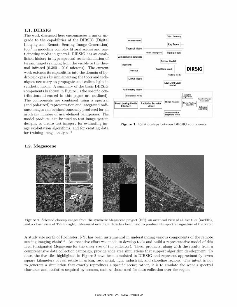
1.1. DIRSIGThe work discussed here encompasses a major up-grade to the capabilities of the DIRSIG (DigitalImaging and Remote Sensing Image Generation)tool1 in modeling complex littoral scenes and par-ticipating media in general. DIRSIG has an estab-lished history in hyperspectral scene simulation ofterrain targets ranging from the visible to the ther-mal infrared (0.380 - 20.0 microns). The currentwork extends its capabilities into the domain of hy-drologic optics by implementing the tools and tech-niques necessary to propagate and collect light insynthetic media. A summary of the basic DIRSIGcomponents is shown in Figure 1 (the specific con-tributions discussed in this paper are outlined).The components are combined using a spectral(and polarized) representation and integrated radi-ance images can be simultaneously produced for anarbitrary number of user-defined bandpasses. Themodel products can be used to test image systemdesigns, to create test imagery for evaluating im-age exploitation algorithms, and for creating datafor training image analysts.4

Figure 1. Relationships between DIRSIG components

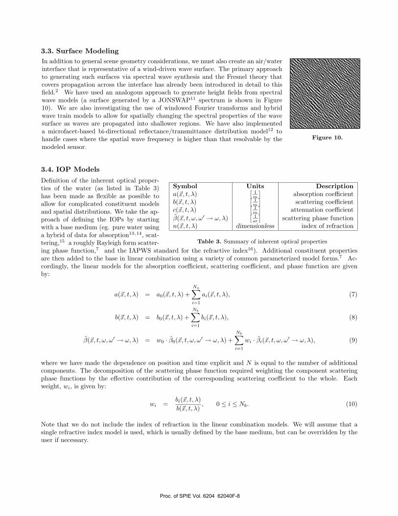
1.2. Megascene

Figure 2. Selected closeup images from the synthetic Megascene project (left), an overhead view of all five tiles (middle),and a closer view of Tile 5 (right). Measured overflight data has been used to produce the spectral signature of the water

.

A study site north of Rochester, NY, has been instrumental in understanding various components of the remotesensing imaging chain5,6. An extensive effort was made to develop tools and build a representative model of thisarea (designated Megascene for the sheer size of the endeavor). These products, along with the results from acomprehensive data collection campaign, provide wide area simulations that support algorithm development. Todate, the five tiles highlighted in Figure 2 have been simulated in DIRSIG and represent approximately sevensquare kilometers of real estate in urban, residential, light industrial, and shoreline regions. The intent is notto generate a simulation that exactly reproduces a specific scene; rather, it is to emulate the scene’s spectralcharacter and statistics acquired by sensors, such as those used for data collection over the region.


I

Figure 3. Tile 5 Topobathymetry

The physics simulating the spectral imaging phenomenology for theterrestrial regions yielded reasonable fidelity.5 Implementation of thetechniques described in this paper enables us to approach the samelevel of simulation fidelity for the coastal region (the so-called Tile5). This area is being being modeled with measured topobathymetry(as shown in Figure 3) and characteristic optical properties. Theresulting simulations will be compared to collected overflight data.

2. BACKGROUND

2.1. Spectral RTE

We use a standard form7 of the spectral radia- i Loss Elastic scattering out of the beamii Loss Inelastic scattering out of the beamiii Loss True absorptioniv Gain Elastic scattering into the beamv Gain Inelastic scattering into the beamvi Gain True Emission into the beam

Table 1. Sources of radiance loss and gain along a beam

tive transfer equation (RTE) incorporating gains andlosses due to the six factors listed in Table 1 and basedon the directed differential radiance at point, x, time,t, and direction, ω. The notation, (ω · ∇)Lλ(x,t,ω,λ)

n(x,t)2 ,is used to represent this derivative, where ∇ is thegradient operator and we have explicitly shown thedependence on the refractive index. Using symbolsfor the inherent optical properties listed in Table 3,we can write the individual contributions as shown in Table 2. The superscript e, i, and s stand for elastic,inelastic, and source (emitted), respectively. Solving for the integrated radiance with all six components andreducing the notation to the single dimension, r, along the ray yields the (simplified) equation,

L∗(rb) =∫ rb

ra

(Le∗(r) + Li

∗(r) + Ls∗(r)

)e−

rbr

c(r′)dr′dr + L∗(ra)e−

rbra

c(r)dr, (1)

where “∗” represents implicit refractive index dependence and the integral is along ray section ra → rb.

This work is primarily concerned with efficiently calculating the elastic scattering corresponding to componentiv (emphasized in Equation 1). The problem of computing inelastic scattering contributions, (component v),can be solved with similar methods, but the added complexity is beyond the scope of this paper.

i (ω · ∇)Lλ(x,t,ω)n(x,t)2 = - be(x, t, λ)Lλ(x,t,ω)

n(x,t)2

ii (ω · ∇)Lλ(x,t,ω)n(x,t)2 = - ai

∗(x, t, λ)Lλ(x,t,ω)n(x,t)2

iii (ω · ∇)Lλ(x,t,ω)n(x,t)2 = - ae(x, t, λ)Lλ(x,t,ω)

n(x,t)2

iv (ω · ∇)Lλ(x,t,ω)n(x,t)2 = + be(x, t, λ)

∫Ωβe(x, t, ω′ → ω, λ)Lλ(x, t, ω′)dω′

v (ω · ∇)Lλ(x,t,ω)n(x,t)2 = + bi(x, t, λ′ → λ)

∫Ω

∫Λβi(x, t, ω′ → ω, λ′ → λ)Lλ′(x, t, ω′)dλ′dω′)

vi (ω · ∇)Lλ(x,t,ω)n(x,t)2 = + So(x, t, ω′)βs(x, t, ω, λ)

Table 2. Contributions to the directional derivative of radiance for the RTE.


2.2. Photon MappingEquation 1 introduced a form of the RTE

Figure 4. Stepwise integration along a ray from ra to rb

that can only be solved numerically exceptin special, and not particularly useful,cases. Stepwise numerical integrationtakes the form of “ray marching”; thatis, the ray along which we are integratingis broken into segments within which weassume that the local optical propertiesand light field influences are invariable.These segments can be of arbitrary lengthand have a center point, rc, which will be the “sample” point from which measurements are made (asdemonstrated in the accompanying figure). In practice, we use an adaptive algorithm to choose segmentsbased on changes in the local volume properties and choose a sample point close to the center point, but witha random offset in order to avoid sampling artifacts. Integration in a highly complex and variable mediumrequires many ray segments and computations, while relatively homogeneous volumes can be traversed ratherquickly.

The integrated form of the in-scattered radiance from a segment centered at point rc and of length ∆rc can bewritten as

Lλ

(rc +

∆rc2, ω

)=

(b (rc, λ)

∫Ω

β (rc, ω′ → ω, λ)Lλ (rc, ω′) dω′)

∆rc, (2)

where we have assumed that the index of refraction does not change significantly within the segment. Given thatthe inherent optical properties are known at point rc (see Section 3.4) at each wavelength λ, the only unknown inthe equation is the radiance coming from all directions ω′. Conceptually, the easiest way to calculate Lλ (rc, ω′)would be to use the same backwards ray tracing process that has been used thus far to compute the contributionfrom the ray. That is, for every direction, ω′, a new ray could be sent out and the radiance contribution couldbe calculated. Since there are an infinite number of directions in Ω, the integral would either have to be solvedusing standard numerical techniques or using a Monte Carlo approach. Within a volume, every new ray thatwould be produced to calculate the integral would also need to do a ray marching integration along its own path.

Diminishing returns eventually limits the effectiveness of sending out numerous new rays and the contributionsof subsequent generations could be approximated or neglected. Nonetheless, the number of operations growsapproximately exponentially as each new generation of rays attempts to calculate the in-scattered radiance. Evenwith a moderate number of samples, a limited number of scattering generations, and large integration step sizes,the calculation is infeasible for any practical application – and we have not even discussed the problem of makingsure that rays eventually “find” the important sources in a scene.

It is therefore impractical to do purely forward (rays from sources) or purely backwards (rays from the detector)calculations for multiple scattering situations. Instead, we adapt a hybrid approach called photon mapping thatcomputes the integral along the ray using a two-pass technique. The photon mapping approach was developedand popularized by Henrik Wan Jensen3 and integrates existing Monte Carlo techniques, an efficient searchalgorithm, and the concept of geometry independent photon storage. It has been used to efficiently producesynthetic, ray-traced images for computer graphics applications. The primary contribution of this work is toadapt this method in order to generate spectral (rather than three band) synthetic imagery driven by bio-opticalmodels of water properties and integrate it into the active and passive sensor testbed already described.

The “photon map” is a collection of discrete bundles of energy (the “photons”) that are organized in a way thatconveniently expresses the spatial relationships between energy bundles (the “map”). Within a particular scene,the photon map is a static entity which contains information about energy in the volume. When ray-tracing ascene, scattering contributions are measured using local density estimates obtained by querying the photon map.These calculations are very efficient, especially compared to Monte Carlo sampling techniques for evaluatingin-scattered radiance.


The first pass of the photon mapping technique consists of generating photons at sources and propagatingthem through the scene. The propagation process is exactly equivalent to established forward Monte Carlotechniques27. As each photon interacts with the volume (through scattering or absorption), a record of thephoton is stored in the map (its position, direction, flux, and wavelength – note that the wavelength cannot bederived from the flux since these are not true photons, only bundles of energy). The photons are stored in ak-d tree,8 independent from any geometry or abstract concept of layers or voxels. The k-d tree is essentiallya binary tree for higher-dimensional data and allows for efficient searching in the next pass. Since the photonmap is only dependent on sources and scene geometry, it is possible to re-use the same photon map for differentsensor locations and orientations.

The second pass consists of backward ray tracing from the detector where the contribution from a ray in a volumeis calculated using the ray marching technique discussed previously. Rather than attempting to calculate thein-scattered radiance directly, we now use the photon map to estimate the in-scattered radiance. Given that weknow the direction, ωi of each photon in the map when it was stored, we can apply the local scattering phasefunction to estimate the amount of flux that is scattering in the direction of the integral. Thus, we transformEquation 2 into,3

Lλ

(rc +

∆rc2, ω

)≈

(1

Vsearch

kλ∑i=1

Φiβ (rc, ωi → ω, λ)

)∆rc, (3)

where kλ is the number of photons found, Vsearch is the volume of the search, and the scattering coefficient hasbeen incorporated into the density estimate. The search volume is usually a sphere that encompasses all of thephotons that were found by a search by radius or number. We will modify this method somewhat in Section 3.5in order to minimize the errors inherent in practical density estimation.

3. APPROACH

3.1. Sampling Algorithms

Any Monte Carlo technique can only be successful if the code that drives it produces samples that are represen-tative of the underlying probability density functions in the model. We divide the process of generating uniformsamples into two steps. During the first step we generate pseudo-random samples from a uniform distributionusing a hybrid approach that combines stratified and Latin hypercube sampling9 in order to guarantee a highlevel of uniformity for any number of samples (see Figure 5).

(a) (b) (c) (d)

Figure 5. Example histograms of two-dimensional samples in the unit square generated from (a) random (by a standardlinear congruential method), (b) stratified, (c) Latin hypercube, and (d) hybrid sampling. Note that while no significantimprovement over stratified sampling can be seen, the hybrid approach gains beneficial uniformity properties from theinclusion of Latin hypercube constraints that are not apparent in these histograms.

Using a uniform sampling of the unit square as a basis, we now project the samples onto a 2-manifold using anarea preserving algorithm that correctly distributes the samples onto the new surface. The projection operatorsare derived using a process compiled from the literature on the subject10 that consists of finding a parametrizationof the manifold, linking the parametrization to the surface area and applying an optional weighting function,


defining and inverting cumulative distribution functions, and forming a new parametrization that takes the unitsquare samples as input. The result is a set of samples on the manifold that have the same uniform distributionproperties as the original samples.

In practice, we use a wide variety of projections to sample anything from arbitrary constructed geometry (usingtriangular facet projections) to hemispheres that are weighted by a bi-directional reflectance distribution function(BRDF). In the next two sections we state, without derivation, two of the simpler sampling projection algorithmsthat are relevant to atmospheric photon generation.

3.1.1. Sphere section sampler projection

-1

-0.5

0

0.5

1

-1 -0.5 0 0.5 1

Figure 6.

A sphere section projection is used to sample a sky dome quadrant by generatinga vector that points to a location within that quadrant for a sphere centered at[0, 0, 0]. Angles θ1, θ2, φ1, and φ2 define the range of zenith and azimuth angles inthe quadrant, respectively (in the equation, µ = cos(θ)). The projected sampledare computed from the two-dimensional uniform random deviates (ξ1,ξ2) as

ψ(ξ1, ξ2) =

⎡⎣ sin(cos−1 (µ1(1 − ξ1) + µ2ξ1)

)cos((φ2 − φ1) · ξ2 + φ1)

sin(cos−1 (µ1(1 − ξ1) + µ2ξ1)

)sin((φ2 − φ1) · ξ2 + φ1)

µ1(1 − ξ1) + µ2ξ1

⎤⎦ (4)

3.1.2. Disk sampler projection

-1

-0.5

0

0.5

1

-1 -0.5 0 0.5 1

Figure 7.

A disk projection is used to sample a solar or lunar disk with radius, ρ. It is simplerto derive the projection on the x-y plane for a uniform disk and then transform thesamples to the proper position defined by the solor/lunar vector and solid angle asretrieved from appropriate ephemeris data for the scene. The projected samples arecomputed as

ψ1(ξ1, ξ2) = ρ√ξ1 · cos(2πξ2),

ψ2(ξ1, ξ2) = ρ√ξ1 · sin(2πξ2) (5)

3.1.3. One-dimensional importance sampling

In addition to two-dimensional projections, we often need a method to ran-domly select a particular element from a set when each element has a weight.Given an arbitrary number of elements, ei, with associated weights, W (ei),the weights are converted to probabilities, P (ei), by dividing by the sum ofall of the weights ( and ),

P (ei) =W (ei)∑iW (ei)

. (6)

The probability elements are ordered so that the largest probability comesfirst in the probability vector (), which helps optimize the next step whenthe probabilities vary. In step , a uniformly distributed random numberr ∈ [0, 1] is pulled from a generator and the value is iteratively compared –this is why we put the larger probabilities first – to the cumulative probabilityof the vector elements. The sampled element is the one corresponding to thelocation of the random number in the vector (element E in the example). Figure 8.


3.2. Photon Generation

For the purposes of this discussion, the source of photons entering the scene is the sky (both the sky dome andthe sun/moon). Nonetheless, the same sampling techniques could be applied to any type of source and used forlow-light level or active sensor modeling.The sky dome (which is a source of down-welled radiance)

Figure 9. Sampling of atmospheric illumination

is broken into quads, each of which is assumed to be ho-mogeneous (i.e. the radiance coming from any point withina quad is the same as any other point in the same quad).Quads are implemented via a sphere section sampler and theweight is equal to the integrated flux coming from the quad(using the area of the current section). All of the quads haveequal area and, therefore, define equal solid angles. The sunand moon disks are constructed using a disk sampler andoriented according to ephemeris tables for the current dateand time. The weight of the solar/lunar disk(s) is the totalintegrated flux coming from the solid angle defined by thedisk. Figure 9 demonstrates how the atmosphere is divided.The zenith, θ, and azimuth, φ, angles are shown.

The entire process of generating photons is summarized inthe list below.

Atmospheric Photon Generation

Initialize a count of “shot photons” to zero

Initialize the photon map with the pre-determined number of photons to be stored Thenumber of photons defined in the preceding twosteps are independent from each other

For each photon, until the photon map is filled,perform the following steps:

Uniformly sample spatially within a pre-determined horizontal extent of the scenethat defines the PropagationArea

Record the sampled point, HorizontalSample Use one-dimensional importance sampling

to select an element of the atmosphere (asky quad or a solar/lunar disk)Weighting is based on the amount of fluxproduced by each element

Sample spatially within the element us-ing a sphere section or disk sampler(see Sections 3.1.1 and 3.1.2, respec-tively) and record the sample position(AtmosphereSample)

Calculate the initial direction of the pho-ton from point to point,PhotonDirection = AtmosphereSample→ HorizontalSample

Use one-dimensional importance samplingto select the wavelength of the photon.Weighting is based on the amount of fluxcontributed by each bandpass for the fluxassociated with the atmosphere element

Propagate the photon through the sceneand store it in the photon map as it is ei-ther absorbed or scattered

Increment the count of shot photons Thephoton count must be incremented regard-less of whether the photon is stored

Calculate the flux associated with each pho-ton by dividing the total flux passing throughthe PropagationArea by the number of pho-tons that were “shot” This is not the numberof photons stored in the map(s)


3.3. Surface ModelingIn addition to general scene geometry considerations, we must also create an air/waterinterface that is representative of a wind-driven wave surface. The primary approachto generating such surfaces via spectral wave synthesis and the Fresnel theory thatcovers propagation across the interface has already been introduced in detail to thisfield.2 We have used an analogous approach to generate height fields from spectralwave models (a surface generated by a JONSWAP11 spectrum is shown in Figure10). We are also investigating the use of windowed Fourier transforms and hybridwave train models to allow for spatially changing the spectral properties of the wavesurface as waves are propagated into shallower regions. We have also implementeda microfacet-based bi-directional reflectance/transmittance distribution model12 tohandle cases where the spatial wave frequency is higher than that resolvable by themodeled sensor.

Figure 10.

3.4. IOP Models

Definition of the inherent optical proper-Symbol Units Descriptiona(x, t, λ)

[1m

]absorption coefficient

b(x, t, λ)[

1m

]scattering coefficient

c(x, t, λ)[

1m

]attenuation coefficient

β(x, t, ω, ω′ → ω, λ)[

1sr

]scattering phase function

n(x, t, λ) dimensionless index of refraction

Table 3. Summary of inherent optical properties

ties of the water (as listed in Table 3)has been made as flexible as possible toallow for complicated constituent modelsand spatial distributions. We take the ap-proach of defining the IOPs by startingwith a base medium (eg. pure water usinga hybrid of data for absorption13,14, scat-tering,15 a roughly Rayleigh form scatter-ing phase function,7 and the IAPWS standard for the refractive index16). Additional constituent propertiesare then added to the base in linear combination using a variety of common parameterized model forms.7 Ac-cordingly, the linear models for the absorption coefficient, scattering coefficient, and phase function are givenby:

a(x, t, λ) = a0(x, t, λ) +Na∑i=1

ai(x, t, λ), (7)

b(x, t, λ) = b0(x, t, λ) +Nb∑i=1

bi(x, t, λ), (8)

β(x, t, ω, ω′ → ω, λ) = w0 · β0(x, t, ω, ω′ → ω, λ) +Nb∑i=1

wi · βi(x, t, ω, ω′ → ω, λ), (9)

where we have made the dependence on position and time explicit and N is equal to the number of additionalcomponents. The decomposition of the scattering phase function required weighting the component scatteringphase functions by the effective contribution of the corresponding scattering coefficient to the whole. Eachweight, wi, is given by:

wi =bi(x, t, λ)b(x, t, λ)

, 0 ≤ i ≤ Nb. (10)

Note that we do not include the index of refraction in the linear combination models. We will assume that asingle refractive index model is used, which is usually defined by the base medium, but can be overridden by theuser if necessary.


3.5. Collection Algorithms

As the number of photons being searched for (or equivalently, the search radius) is increased, we increase therisk of finding photons uncharacteristic of the local light field. We want to grow the search so we can drive downthe variance inherent in the photon map due to the random, sampled nature of construction (despite using veryuniform sampling strategies). The objective of the collection algorithms that follow is to find an efficient meansof extending the search volume (to reduce noise) while maintaining the assumption of locality. There are manyplausible and potentially more accurate approaches to compensating for the two sources of error presented here(boundary and spectral). Our goal in developing these methods is to make the process as efficient as possiblewhile still compensating for the bulk of the error.

3.5.1. Boundary collection algorithm (Boundary map)

By far, the largest errors are likely to occur near boundaries of the volume where the search radius can extendbeyond the bounds of the volume. This is also the region where, at least for turbid media, the most scatteringwill occur. Since the photon map has no internal concept of boundaries, it will treat anything beyond a boundaryas part of the local volume. In most cases, this ends up causing the density estimate to be biased lower thanit should be due to the effective inclusion of a photon “void” in the density estimate. To compensate for thiserror, we construct a “boundary map” (analogous to a photon map) composed of nodes containing the distanceto the boundaries of the volume at that particular point. These nodes are computed and stored during thefirst pass of the algorithm. The boundary map is constructed using a sparsely populated k-d tree which can besearched to estimate the location of boundaries from the local boundary nodes. Once these distances are known,an effective volume can be calculated. Within a complex scene it is possible for boundaries to be arbitrarilyoriented, however, we assume that it is sufficient to know the boundary distances in the six axial directions andto be conservative in our estimates of the constraints.

We will consider the volume of a sphere that has been constrained in any combination

Figure 11.

of six specified directions. These six directions correspond to the positive and negativeorthogonal axial directions centered at the sphere origin (the search site). The axeswould presumably be aligned with the global coordinate system though this is notnecessary. If the original search sphere does not hit a boundary in a particulardirection then the constraint is zero and the search sphere was able to expand to itsfull radius in that direction (whether or not it found nodes at that distance). Eachconstraint is also less than the search radius, R, since the search site must be withinthe boundary. This gives each constraint a possible range of [0, R).

In order to calculate the effective search volume, the volumes outside of the bound-aries (the occluded volumes) must be removed from the volume of the unconstrainedsphere. In the simplified case of a single constraint, the effective volume can be foundby removing a spherical cap corresponding to the constraint. When there is more than one constraint and thespherical caps intersect we need to account for removing the intersected volumes (a conceptual rendering of sixintersecting constraints is shown). Given the level of symmetry in the types of intersections possible we canpre-compute the intersecting volumes at selected intervals in order to optimize the volume calculation.

3.5.2. Spectral collection algorithm

Accounting for spectral photons for multi/hyperspectral modeling introduces an effective bias error incurred bysearching for enough photons in each spectral band to drive down the spectral noise. Under ideal conditions, weexpect that the total variance in the estimate is linearly related to the number of photons that are used to formthe estimate. Accordingly, under optimal circumstances where the photons are uniformly distributed across allof the spectral bands, we expect that the spectral variance will increase by a factor of s, where s is the numberof spectral bands. In other words, to maintain the same level of variance as we would have without consideringspectral photons, we need to search for s · N rather than N . This makes us more susceptible to errors as weviolate the locality assumption. The approach we take to compensate for this source of error is to perform atwo-step search.


The first step is to perform a local core search by radius across all spectral bands. The radius is set so thatthe assumption of a local volume is reasonably met. The density that results from this search is used to set themean density of the final spectral density (no spectral shape exists at the moment). Thus, we ensure that thefinal integrated density will be consistent with the local light field intensity.

The second step performs an expanded spectral search within each spectral band. The number of spectralphotons to find is set such that we ensure a certain level of fidelity. We also calculate the relative weight of eachspectral density and apply this weight to the core density calculated in the previous step (a variety of methodscan be used here). The spectral density that results is our final estimate.

4. VALIDATION

For any model of this size and complexity it is necessary to consider both the theoretical and procedural validityof the model. We have adopted, and are currently carrying out, an intensive validation process for the modelconsisting of five phases of increasing complexity. The validation process is summarized in Table 4.

Phase Type Description

I Code Extensive numerical algorithm testing, step-by-step ray tracing,and optimization

II Intuitive Design and rendering of a series of simple test scenes which can bejudged based on visual inspection

III IOP⇔AOP Examines apparent optical properties for which an approximaterelationship to IOPs is known17,18

IV Peer-to-peer Comparison against Hydrolight for fully modeled illumination,IOP, and surface models19

V Sub-space Examines the correspondence between synthetic invariant targetsub-spaces20 and measured targets in the Megascene Tile 5 region

Table 4. Validation phases

5. APPLICATIONS

The potential applications of this tool are multiple and varied and include:

• Passive broadband/multispectral/hyperspectral sensor design and sensitivity studies

• Radiometric instrument design and testing

• Evaluation of existing sensors under various environmental conditions to determine operational limits andoptimum conditions for data acquisition

• Studies of sensor design tradeoffs with respect to cost per sensor, coverage, and data quality

• Thermal modeling (using DIRSIG’s built-in thermal model and weather histories)

• Surface, partially submerged, and fully submerged target detection algorithm design and evaluation

• Spatially variant bio-luminescence studies

• LIDAR simulation (using DIRSIG’s built-in LIDAR model along with photon mapping capabilities)

• Low-light level simulation using above-water or submerged illumination sources

• Geometric obscuration studies coupled with temporal illumination study

• Studies on the impact of adjacency effects on target detection


• Multi-scale collection scenario design and mission planning

• As a sensor fusion testbed where a simulated host of sensors across the EM spectrum provide a baseline ofimage data sets to best present unique imaging phenomenologies to a user or algorithm

• Background signature characterization

• Invariant sub-space construction for target detection algorithms20

6. SUMMARY

The photon-mapping technique and its extension into the hyperspectral domain shows great potential in ad-dressing basic hydrologic optical phenomenology in the littoral region including embedded targets and plat-form/instrument obscuration of the scene. Prior to this implementation, approaches that could simulate littoralscenes relied on assumptions that limited the model’s capabilities and usability. The stochastic nature of a MonteCarlo solution coupled with the extreme scales between scene and sensor renders classic techniques prohibitivelycomputationally demanding when considering scattering media. Photon mapping optimizes the computation ofin-scattered radiance through an efficient photon searching and radiance estimation and brings such simulationtools closer to operational viability for flexible, multi-scale usage.

The integration of these techniques into the DIRSIG environment makes it possible to address many issues inport and harbor security by using an extensive collection of sensor, environmental, geometric, and radiativetransfer models and tools. Extensive validation of both overhead, surface, and underwater simulations againstboth modeled and measured data will be used to verify subjective phenomenology as well as radiometric accuracyand fidelity. Finally, simulation of the the Megascene Tile 5 littoral zone will provide a large scale project forwhich expansive ground truth data has been collected.

ACKNOWLEDGMENTS

Support for this work has been provided by the Department of Defense Office of Naval Research under a Multidis-ciplinary University Research Initiative (MURI) (N00014-01-1-0867): Model-based Hyperspectral ExploitationAlgorithm Development.

REFERENCES1. E. Ientilucci and S. Brown, “Advances in wide area hyperspectral image simulation,” in Proceedings of the

SPIE conference on Targets and Backgrounds IX: Characterization and Representation, 5075, pp. 110–121,(Orlando, FL), April 2003.

2. C. R. Bostater, “Hyperspectral simulation and recovery of submerged targets in turbid waters,” in Proceed-ings of the SPIE, 5780.

3. H. W. Jensen, Realistic Image Synthesis Using Photon Mapping, A K Peters, 2001.4. Digital Imaging and Remote Sensing Laboratory, DIRSIG User’s Manual, February 2006.5. N. G. Raqueno, L. E. Smith, D. W. Messinger, C. Salvaggio, R. V. Raqueno, and J. R. Schott, “Megacollect

2004: Hyperspectral collection experiment of terre strial targets and backgrounds of the RIT Megasceneand surrounding area (Rochester, New York),” in Proceedings of the SPIE conference on Algorithms andTechnologies for Multispectral, Hyperspectral, and Ultraspectral Imagery XI, (Orlando, FL), March 2005.

6. R. Raqueno, N. Raqueno, A. Vodacek, J. Schott, A. Weidemann, S. Effler, M. Perkins, W. Philpot, andM. Kim, “Megacollect 2004: Hyperspectral collection experiment over the waters of the rochester embay-ment,” in Proceedings of the SPIE conference on Algorithms and Technologies for Multispectral, Hyperspec-tral, and Ultraspectral Imagery XI, (Orlando, FL), March 2005.

7. C. Mobley, Light and Water: Radiative Transfer in Natural Waters, Academic Press, Boston, MA, 1994.8. J. L. Bentley, “Multidimensional search trees used for associative searching,” Communications of the

ACM 18, pp. 509–517, September 1975.9. Chiu, Shirley, and Wang, Multi-jittered Sampling. Graphics Gems IV, Academic Press, 1993.


10. J. Arvo, “Stratified sampling of 2-manifolds,” Monte Carlo Ray Tracing, SIGGRAPH 2003 Course Notes ,pp. 39–61, 2003.

11. D. E. Hasselmann, M. Dunckel, and J. A. Ewing, “Directional wave spectra observed during JONSWAP1973,” Journal of Physical Oceanography , pp. 1264–1280, 1980.

12. M. Ashikhmin, S. Premoze, and P. Shirley, “A microfacet-based BRDF generator,” in Siggraph 2000, Com-puter Graphics Proceedings, K. Akeley, ed., pp. 65–74, ACM Press / ACM SIGGRAPH / Addison WesleyLongman, 2000.

13. R. M. Pope and E. S. Fry, “Absorption spectrum (380-700 nm) of pure water. ii. integrating cavity mea-surements,” Appl. Opt. 36, pp. 8710–8723, 1997.

14. R. C. Smith and K. Baker, “Optical properties of the clearest natural waters,” Applied Optics 20(2),pp. 177–184, 1981.

15. H. Buiteveld, J. M. H. Hakvoort, and M. Donze, “The optical properties of pure water,” SPIE Proceedingson Ocean Optics XII 2258, pp. 174–183, 1994.

16. International Association for the Properties of Water and Steam, Release on the Refractive Index of OrdinaryWater Substance as a Function of Wavelength, Temperature and Pressure, September 1997.

17. H. R. Gordon, O. B. Brown, and M. M. Jacobs, “Computed relationships between the inherent and apparentoptical properties of a flat homogeneous ocean,” Applied Optics 14, pp. 417–427, 1975.

18. J. T. O. Kirk, The relationship between inherent and optical properties. Ocean Optics, Oxford UniversityPress, New York, 1994.

19. C. D. Mobley and L. K. Sundman, Hydrolight 4.1 Technical Documentation. Redmond, WA 98052,Aug. 2000.

20. G. Healey and D. Slater, “Models and methods for automated material identification in hyperspectralimagery acquired under unknown illumination and atmospheric conditions,” IEEE Trans. Geosci. RemoteSensing 97(6), pp. 2706–2717, 1999.


A exible hyperspectral simulation tool for complex ...cnspci/references/goodenough2006.pdf · Adam...

Documents

Transcript of A exible hyperspectral simulation tool for complex ...cnspci/references/goodenough2006.pdf · Adam...