A DYNAMIC ROUTING MODEL

Dynamic Routing Model and Solution Methods for Fleet Management with Mobile Technologies

Bernard K.-S. Cheung GERAD and Ecole Polytechnique de Montreal

C.P. 6079, succ Centre-ville Montreal, Quebec, Canada H3C 3A7

Email: [email protected]

K.L. Choy Department of Industrial and Systems Engineering

The Hong Kong Polytechnic University Hung Hom, Kowloon, Hong Kong


Chung-Lun Li*

Revised: 14 August 2007

Department of Logistics



John W.Z. Shi Department of Land Surveying and Geo-Informatics



Jian Tang School of Remote Sensing and Information Engineering

Wuhan University 29 Luoyu Road, Wuhan, Hubei, P.R.China 430079


4 January 2007

* Corresponding author

This is the Pre-Published Version.

Abstract

We develop and analyze a mathematical model for dynamic fleet management that captures

the characteristics of modern vehicle operations. The model takes into consideration dynamic

data such as vehicle locations, travel time, and incoming customer orders. The solution

method includes an effective procedure for solving the static problem and an efficient re-

optimization procedure for updating the route plan as dynamic information arrives.

Computational experiments show that our re-optimization procedure can generate near-

optimal solutions.

Keywords: Dynamic vehicle routing; heuristics; mobile technologies

1

1. INTRODUCTION

With the advances of mobile and information technologies, dynamism has become a key

feature of today’s logistics operations environment. However, a major limitation of many

traditional vehicle management systems is their inability to re-plan transportation operations

satisfactorily when facing dynamic data. Motivated by the characteristics of the new

communication technologies, such as radio frequency identification (RFID), global positioning

systems (GPS), and geographical information systems (GIS), in this paper we develop and

analyze a mathematical model for dynamic fleet management that attempts to capture the

characteristics of modern vehicle operations.

With the use of RFID, data such as identity, volume, and types of stock keeping units of

each customer order can be accurately recorded and tracked. Such technologies can lead to the

real-time update of information of new customer orders, including their expected arrival time

at the pickup locations, their vehicle capacity consumption, their delivery requirements, due

dates, etc. These are translated into dynamic demand data in the vehicle scheduling system.

The use of GPS and GIS can provide real-time data on the vehicle locations, spatial

distribution of roads and related facilities, and road conditions. GIS can further be used for

managing, querying, and analyzing spatial related data for fleet analysis. The real-time data

obtained from the GPS/GIS are translated into dynamic data on the vehicle’s travel time for

each transportation segment, as well as the vehicle’s travel time from its current position to its

next pickup or drop-off point. The tracking feature of an advanced vehicle scheduling system

can also provide dynamic data on the load level of each vehicle. In order to make good use of

these dynamic data, a robust vehicle management system needs to either periodically or

dynamically update the route plan, while the updating process has to be performed with high

efficiency. In this paper, we propose a vehicle routing framework which takes into account the

dynamism of data as well as the efficiency of the route-plan updating process.

Our proposed framework requires us to determine a route plan through solving a static

vehicle routing problem before the start of the daily operation. It also requires us to make

dynamic changes of the routing whenever new information is obtained throughout the day. We

develop a mathematical model for such a dynamic vehicle routing framework. This

mathematical model includes solving a static problem as well as a problem for dynamic change

of the route plan. We propose heuristic solution methods for both the static and dynamic

problems. The heuristic for the static problem emphasizes effectiveness. It includes the

development of an initial feasible solution using the idea of “seed selection” (see Fisher and

Jaikumar 1981), as well as the refinement of the solution via local search techniques and a

2

genetic algorithm. The heuristic for the dynamic problem emphasizes efficiency. The design of

our solution methods is therefore customized for the vehicle routing setting where advanced

mobile technologies are employed.

Real-time vehicle routing has been studied by a number of researchers. Psaraftis (1995),

Gendreau and Potvin (1998), and Ghiani et al. (2003) have conducted recent surveys on this

topic. More recent developments in this area include the following: Yang et al. (2004) and

Chen and Xu (2006) have developed mathematical-programming-based algorithms for

different variants of the dynamic vehicle routing model. Larsen et al. (2002), Attanasio et al.

(2004), Liao (2004), Van Hemert and La Poutre (2004), Du et al. (2005), Montemanni et al.

(2005), Tang and Hu (2005), Fabri and Recht (2006), and Potvin et al. (2006) have developed

various rule-based and local search techniques, such as insertion methods, tabu search, ant

colony optimization, intra-route improvement, inter-route improvement, etc., for dynamic

vehicle routing. Godfrey and Powell (2002a,b), Hu et al. (2003), Bent and Van Hentenryck

(2004), Larsen et al. (2004), and Thomas and White (2004) have used “look-ahead”

approaches to tackling the dynamism of real-time routing problems. They try to incorporate

probabilistic characteristics of future events into decision making, Mitrovic-Minic et al. (2004),

Mitrovic-Minic and Laporte (2004), and Branke et al. (2005) have analyzed waiting strategies

for vehicles that are already under way when they face dynamic customer order arrivals.

Fleischmann et al. (2004) have presented a planning framework for dynamic vehicle routing.

Our research differs from the above-mentioned works in that we focus on the development of a

solution method that takes into consideration both the effectiveness of the static route plan and

the efficiency of the re-planning procedure, and we consider the dynamic data of the vehicle

position, load level of each vehicle, travel time, and the status of the customer orders.

The rest of the paper is organized as follows: In the next section, we describe our

problem in detail. The solution method for the static problem is developed in Section 3. In

Section 4, the dynamic updating routine is presented and computational results are presented.

Some concluding remarks are provided in Section 5.

2. PROBLEM DESCRIPTION

We consider a directed transportation network )},0{( ANG ∪= , where },,2,1{ nN = is the

set of customer locations, 0 is the central depot of vehicles, and A is the set of arcs. For any

arc Aji ∈→ , let ijτ denote the normal (minimum) travel time from node i to node j . The

actual travel time between these two nodes, denoted as ijt , will be updated dynamically over

3

time, where ijijt τ≥ . There are m identical vehicles available, where each of them has a

capacity K . Each customer order is represented by ijd , which is the amount of goods to be

picked up at node i and delivered to node j , where 0=ijd if such an order does not exist. For

simplicity, we assume that every node is either a pickup node of exactly one customer order or

a delivery node of exactly one customer order, but not both. In reality, if there are two or more

pickups/deliveries taking place at the same location i , then we will transform the problem into

our model by duplicating node i into multiple nodes and assigning a node to each

pickup/delivery requirement. Also, if there is a node which is neither a pickup node nor a

delivery node, then we can eliminate it from the network and update the ijt values accordingly.

Hence, at any point in time, if there are q customer orders to be satisfied, then network G

contains 12 += qn nodes (i.e., one pickup node and one delivery node for each order, plus a

node 0 for the central depot). Once a customer order is delivered, the pickup and delivery

nodes of that order will be removed from the network.

For each customer order ijd , there is a given pair of time windows ],[ Pij

Pij sr and ],[ D

ijD

ij sr ,

where parameter Pijr is the earliest pickup time of order ijd at node i , parameter P

ijs is the

latest pickup time of order ijd at node i , parameter Dijr is the earliest delivery time of order ijd

at node j , and parameter Dijs is the latest delivery time of order ijd at node j . We assume that

each customer order has to be picked up and delivered by a single vehicle (i.e., order splitting

is not allowed). The vehicle has to arrive at the pickup location of an order no later than the

latest pickup time. In case it arrives at the pickup location before the earliest pickup time, it can

wait at that location until the goods are ready for pickup. Similarly, the vehicle has to arrive at

the delivery location no later than the latest delivery time of the order. Waiting is allowed in

case it arrives at the delivery location early. All vehicles are initially located at the central

depot, and they have to return to the depot after they finish their pickup and delivery tasks. We

assume that the loading and unloading time of goods is negligible at the pickup and delivery

locations.

In reality, the earliest pickup time Pijr represents the ready time of the order at the pickup

location. For example, the order may be arriving at the pickup location via another

transportation mode. However, with the real-time order-tracking capability of the RFID-based

system, the ready time of this order at its pickup location can be determined well in advance.

The latest pickup time Pijs represents the deadline for the order pickup. If there is no such

deadline, then we set +∞=Pijs . The latest delivery time D

ijs represents the deadline for the

arrival of the goods at the delivery location as specified by the customer. The earliest delivery

time Dijr is the earliest possible time that the customer would like the goods to arrive at the

4

delivery point. If there is no such requirement, then we set 0=Dijr .

Our problem is to determine a set of m vehicle routes such that (i) the total amount of

goods carried by each vehicle is no more than K at any point in time; (ii) the pickup of an

order must precede its delivery; (iii) the time-window constraints of all customer orders are not

violated; and (iv) the total travel time (excluding idle time) of the m vehicles is minimized.

The total vehicle travel time is chosen as our objective as an approximation of the total cost of

operation, which includes fuel cost, driver cost, equipment depreciation, and other intangible

costs. In fact, it is not difficult to modify our solution method to handle other cost-

minimization objectives.

The implementation of our dynamic pickup and delivery routing system is done as

follows: At the beginning of a day, the system determines a route plan based on the normal

travel times and demand data available on hand. This requires the determination of a solution

to the “static” pickup and delivery vehicle routing problem with time windows. The system

may spend a substantial amount of time on determining the route plan. Hence, we develop a

sophisticated heuristic procedure for solving this static problem. The details of the heuristic

procedure are provided in Section 3. Dynamic data arrive throughout the course of the day.

They include the change in traffic conditions captured by the GPS, which results in a change of

travel time ijt , as well as the arrivals of new customer orders. When new travel time data arrive,

the system will update and re-optimize the route plan. When a new customer order arrives, the

system will also attempt to update the route plan immediately to determine if the order should

be accepted (the order will be rejected if no feasible route plan can be identified). Once the

new customer order is accepted, the system will re-optimize the route plan. This kind of re-

optimization must be done quickly with minimal computational time, say within 30 seconds. In

particular, when a new customer order arrives, a “near real-time” response is more desirable.

Therefore, we develop an efficient procedure for the re-optimization. The details of the

procedure are presented in Section 4.

3. SOLUTION METHOD FOR THE STATIC PROBLEM

The heuristic solution procedure for the static problem is divided into two phases. In the first

phase, an initial population of feasible solutions is generated. This is done by constructing a

population of initial feasible solutions via a “seed selection” approach (Section 3.1), followed

by an application of a solution refinement procedure (Section 3.2) to improve each initial

feasible solution. In the second phase, the solution population is improved by a genetic search

5

routine, and a final solution is selected (Section 3.3).

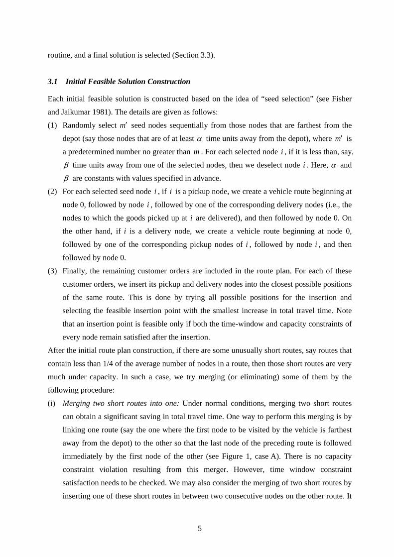
3.1 Initial Feasible Solution Construction

Each initial feasible solution is constructed based on the idea of “seed selection” (see Fisher

and Jaikumar 1981). The details are given as follows:

(1) Randomly select m′ seed nodes sequentially from those nodes that are farthest from the

depot (say those nodes that are of at least α time units away from the depot), where m′ is

a predetermined number no greater than m . For each selected node i , if it is less than, say,

β time units away from one of the selected nodes, then we deselect node i . Here, α and

β are constants with values specified in advance.

(2) For each selected seed node i , if i is a pickup node, we create a vehicle route beginning at

node 0, followed by node i , followed by one of the corresponding delivery nodes (i.e., the

nodes to which the goods picked up at i are delivered), and then followed by node 0. On

the other hand, if i is a delivery node, we create a vehicle route beginning at node 0,

followed by one of the corresponding pickup nodes of i , followed by node i , and then

followed by node 0.

(3) Finally, the remaining customer orders are included in the route plan. For each of these

customer orders, we insert its pickup and delivery nodes into the closest possible positions

of the same route. This is done by trying all possible positions for the insertion and

selecting the feasible insertion point with the smallest increase in total travel time. Note

that an insertion point is feasible only if both the time-window and capacity constraints of

every node remain satisfied after the insertion.

After the initial route plan construction, if there are some unusually short routes, say routes that

contain less than 1/4 of the average number of nodes in a route, then those short routes are very

much under capacity. In such a case, we try merging (or eliminating) some of them by the

following procedure:

(i) Merging two short routes into one: Under normal conditions, merging two short routes

can obtain a significant saving in total travel time. One way to perform this merging is by

linking one route (say the one where the first node to be visited by the vehicle is farthest

away from the depot) to the other so that the last node of the preceding route is followed

immediately by the first node of the other (see Figure 1, case A). There is no capacity

constraint violation resulting from this merger. However, time window constraint

satisfaction needs to be checked. We may also consider the merging of two short routes by

inserting one of these short routes in between two consecutive nodes on the other route. It

6

may help to avoid time window constraint violation, but the vehicle may have to be

checked for overloading at the insertion point. We can only be sure of substantial saving if

these two routes to be merged are sufficiently close to each other, or if there is a

considerably wide gap between these two consecutive nodes (see Figure 1, case B).

(ii) Eliminating unusually short routes: If the route plan contains some unusually short routes

(say routes with no more than three pairs of pickup and delivery nodes), we transfer all the

pairs of pickup-delivery nodes to the other routes, provided that all constraints are

satisfied and that the total travel time is reduced after this transfer.

3.2 A Solution Refinement Procedure

The purpose of the refinement procedure is to improve the initial feasible solution generated by

the method described in Section 3.1. The procedure includes two parts. These two parts are

applied alternately and iteratively until a limit on the computational time (say 1 minute for a

network up to 400 nodes) is reached:

(1) Refinement within each route: This is done by transferring a node from its current position

to another position on the vehicle route. The position that this node is being transferred to

is selected in such a way that: (i) if the node is a pickup node, then it must precede the

corresponding delivery node in the new vehicle route; (ii) if the node is a delivery node,

then it must be preceded by the corresponding pickup node in the new vehicle route;

(iii) the new route plan must satisfy all time-window constraints; (iv) the new route plan

must satisfy the vehicle capacity constraint; and (v) the improvement in total travel time is

maximized (among all the feasible choices). Such a refinement technique is known as

“Or-opt” (see Golden and Stewart 1985).

(2) Refinement between two routes: This is done by transferring a customer order (i.e., a pair

of pickup and delivery nodes) from one vehicle route to another. Again, this is done in

such a way that all pickup and delivery precedence constraints, time-window constraints,

and vehicle capacity constraint are not violated, and the selection of the locations for this

pair of pickup and delivery nodes is made in such a way that the improvement in total

travel time is maximized.

3.3 Solution Enhancement by Genetic Search Method

Since the problem size of our model is usually quite large in practice, construction of a limited

number of feasible solutions followed by subsequent refinements may not be sufficient to

attain global optimality, as the total number of possible assignments is almost inexhaustible.

7

Hence, the application of a genetic search method may help in getting a very good solution,

and hopefully close to the true optimum. We now present a Genetic Algorithm (GA), which

takes the population of feasible solutions generated by the first phase as input and iteratively

improves it. The efficiency of the GA is enhanced by some well-proven modifications (see

Cheung et al. 2001 and Cheung 2005). The following is a description of the modified GA:

(1) Encoding method: We represent a chromosome by a list of customer orders along with

their vehicle route assignment. That is, a chromosome is denoted as

}0|),,{( >=∆ ijij dji δ , where kij =δ if customer order ijd is served by the k th vehicle

route. We refer to each element ),,( ijji δ as a “gene” and ijδ as the value of the gene. For

example, consider the problem instance shown in Figure 2(a). The route assignment

corresponding to chromosome A depicted in Figure 2(b) is {(1,2,1), (3,6,2), (4,5,2),

(7,8,1), (9,10,2), (11,12,2)}.

(2) Fitness evaluation: The fitness of a chromosome is determined as follows: We

heuristically construct each vehicle tour. This is done by first selecting the farthest node as

the seed node and then applying steps (2) and (3) of the seed selection algorithm (Section

3.1) to construct a feasible tour. This is followed by step (1) of the solution refinement

procedure (Section 3.2). Then, the fitness of the chromosome is given by the total travel

time of all vehicles in the constructed solution. For example, consider chromosome A as

shown in Figures 2(b) and 2(c). The initial route plan of this chromosome is obtained by

constructing a feasible route plan with three routes choosing nodes 2, 6, and 5 as seeds.

The resulting route plan, which includes routes 087210 →→→→→ and

0121110965430 →→→→→→→→→ , is obtained through merging two shortest

routes. Route 1 has a length of 432 (minutes), and route 2 has a length of 452 (minutes). In

this case, the fitness value of the chromosome is 884.

(3) The uniform crossover operations: The crossover operation involves exchanging gene

values in a subset of randomly selected entries between a pair of chromosomes. This is

done as follows: First, a pair of chromosomes is randomly selected. Second, a positive

integer },,2,1{ qh ∈ is randomly generated and h entries are randomly selected, where

q is the number of customer orders. We swap the gene values between this pair of

chromosomes at all of the selected entries. These two newly produced solutions

(chromosomes) are evaluated and compared with the fitness values of their parents. If the

fitness value of one of these new chromosomes produced are found to be better than both

of its parents, we discard the parents and replace them by their offspring. Otherwise, we

keep the parents. To avoid redundancy and to enhance the effectiveness of the procedure,

8

we will perform this crossover operation only if the corresponding gene values of at least

two of the selected entries are distinct. For example, suppose that the pair of chromosomes

selected are chromosome A = {(1,2,1), (3,6,2), (4,5,2), (7,8,1), (9,10,2), (11,12,2)} and

chromosome B = {(1,2,1), (3,6,2), (4,5,3), (7,8,2), (9,10,1), (11,12,3)} as shown in Figures

2(b) and 2(c). Suppose 2=h and that the fourth and fifth entries are selected. Then, the

offspring are chromosome C = {(1,2,1), (3,6,2), (4,5,2), (7,8,2), (9,10,1), (11,12,2)} and

chromosome D = {(1,2,1), (3,6,2), (4,5,3), (7,8,1), (9,10,2), (11,12,3)}. Since the first

offspring is better than both parents (see Figure 2(c)), we replace both parents by the two

offspring. In our genetic search procedure, we repeat the crossover operation for a pre-

specified number of pairs of chromosome in the population. Here in our example as shown

in Figure 2, the best solution is chromosome C with the fitness value found to be 851.

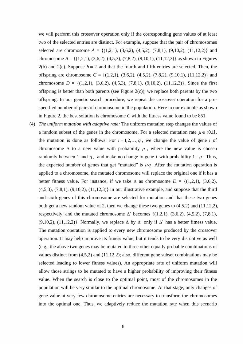
(4) The uniform mutation with adaptive rate: The uniform mutation step changes the values of

a random subset of the genes in the chromosome. For a selected mutation rate ]1,0(∈µ ,

the mutation is done as follows: For qi ,,2,1 = , we change the value of gene i of

chromosome ∆ to a new value with probability µ , where the new value is chosen

randomly between 1 and q , and make no change to gene i with probability µ−1 . Thus,

the expected number of genes that get “mutated” is qµ . After the mutation operation is

applied to a chromosome, the mutated chromosome will replace the original one if it has a

better fitness value. For instance, if we take ∆ as chromosome D = {(1,2,1), (3,6,2),

(4,5,3), (7,8,1), (9,10,2), (11,12,3)} in our illustrative example, and suppose that the third

and sixth genes of this chromosome are selected for mutation and that these two genes

both get a new random value of 2, then we change these two genes to (4,5,2) and (11,12,2),

respectively, and the mutated chromosome ∆′ becomes {(1,2,1), (3,6,2), (4,5,2), (7,8,1),

(9,10,2), (11,12,2)}. Normally, we replace ∆ by ∆′ only if ∆′ has a better fitness value.

The mutation operation is applied to every new chromosome produced by the crossover

operation. It may help improve its fitness value, but it tends to be very disruptive as well

(e.g., the above two genes may be mutated to three other equally probable combinations of

values distinct from (4,5,2) and (11,12,2); also, different gene subset combinations may be

selected leading to lower fitness values). An appropriate rate of uniform mutation will

allow those strings to be mutated to have a higher probability of improving their fitness

value. When the search is close to the optimal point, most of the chromosomes in the

population will be very similar to the optimal chromosome. At that stage, only changes of

gene value at very few chromosome entries are necessary to transform the chromosomes

into the optimal one. Thus, we adaptively reduce the mutation rate when this scenario

9

occurs. Specifically, we gradually reduce the mutation rate, for instance, from 0.2 to 0.1

after each 100 generations.

(5) The selection scheme and termination criteria: The selection of chromosomes for an

improved population after each generation (i.e., after all the crossover and mutation

operations) is made according to the steps described in (3) and (4). It is also important to

update the solution with the best fitness value at each generation. The iteration will stop

after a pre-specified number of generations, while this number can be determined through

some trial runs with examples.

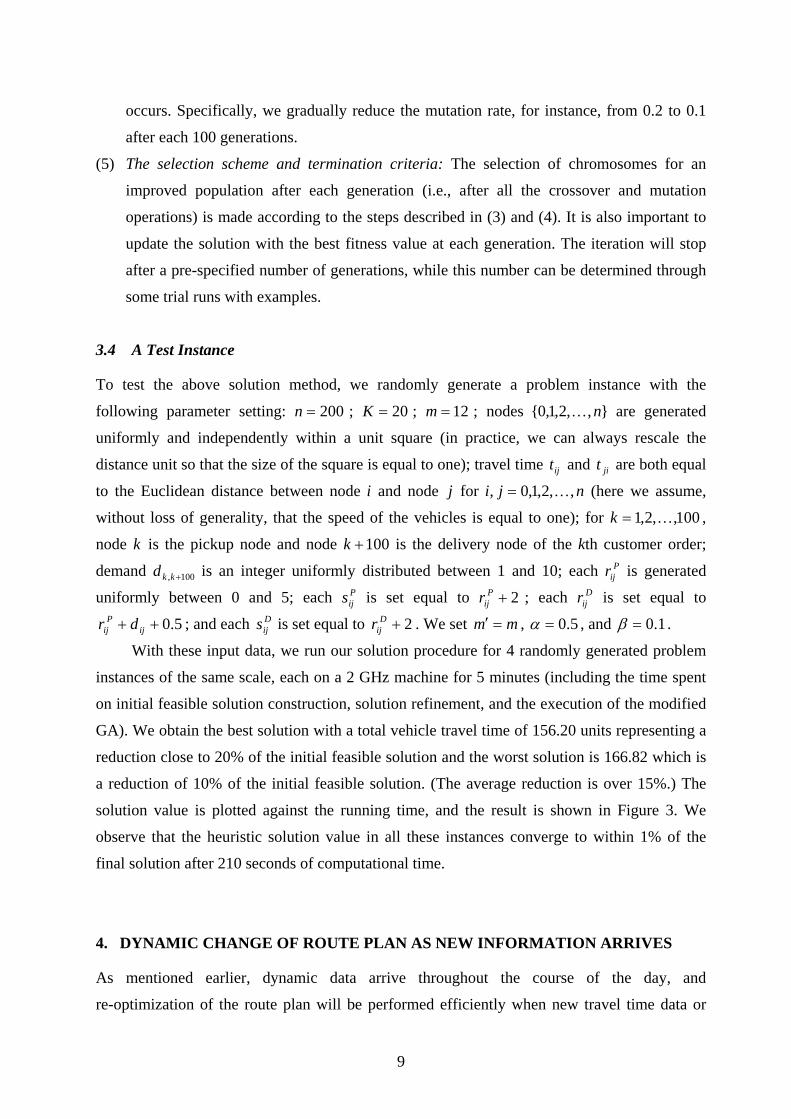
3.4 A Test Instance

To test the above solution method, we randomly generate a problem instance with the

following parameter setting: 200=n ; 20=K ; 12=m ; nodes },,2,1,0{ n are generated

uniformly and independently within a unit square (in practice, we can always rescale the

distance unit so that the size of the square is equal to one); travel time ijt and jit are both equal

to the Euclidean distance between node i and node j for nji ,,2,1,0, = (here we assume,

without loss of generality, that the speed of the vehicles is equal to one); for 100,,2,1 =k ,

node k is the pickup node and node 100+k is the delivery node of the kth customer order;

demand 100, +kkd is an integer uniformly distributed between 1 and 10; each Pijr is generated

uniformly between 0 and 5; each Pijs is set equal to 2+P

ijr ; each Dijr is set equal to

5.0++ ijP

ij dr ; and each Dijs is set equal to 2+D

ijr . We set mm =′ , 5.0=α , and 1.0=β .

With these input data, we run our solution procedure for 4 randomly generated problem

instances of the same scale, each on a 2 GHz machine for 5 minutes (including the time spent

on initial feasible solution construction, solution refinement, and the execution of the modified

GA). We obtain the best solution with a total vehicle travel time of 156.20 units representing a

reduction close to 20% of the initial feasible solution and the worst solution is 166.82 which is

a reduction of 10% of the initial feasible solution. (The average reduction is over 15%.) The

solution value is plotted against the running time, and the result is shown in Figure 3. We

observe that the heuristic solution value in all these instances converge to within 1% of the

final solution after 210 seconds of computational time.

4. DYNAMIC CHANGE OF ROUTE PLAN AS NEW INFORMATION ARRIVES

As mentioned earlier, dynamic data arrive throughout the course of the day, and

re-optimization of the route plan will be performed efficiently when new travel time data or

10

new customer orders arrive. Let t be a time epoch at which new data arrive. The following are

the crucial data required in order to perform the re-optimization:

(i) the position of each vehicle at time t and the vehicle’s travel time to the next node;

(ii) the load level of each vehicle at time t ;

(iii) the status of each customer order at time t ; and

(iv) the travel time of each arc at time t .

We now describe how the re-optimization is performed heuristically. We first consider

the case in which a new customer order has arrived. In this case, we create a new pickup node

i and a new delivery node j for this new order, and the new customer order is denoted as ijd .

We attempt to add this new order to an existing route. We need to determine the best possible

insertion points for i and j . To do that, we search through all existing routes and all possible

pairs of insertion points, check the feasibility of each possible insertion, and evaluate the

impact of the insertion. If the number of vehicle routes in the current solution is less than m ,

then one of the candidates in this search is obtained by creating a new route that serves only

this new customer order. This step is followed by the application of the refinement procedure

described in Section 3.2 to further improve the solution. Next, we consider the case in which

new travel time data have arrived. In this case, if the new travel time does not cause

infeasibility of the current route plan, then we simply apply the refinement procedure described

in Section 3.2 to improve the solution. If the new travel time does cause infeasibility of the

current route plan, then remove those infeasible orders and reinsert them into the route plan

(i.e., treat them as newly arrived orders). When the refinement procedure is applied upon

arrival of new information, a very short computational time limit (say within 30 seconds) is set

so that the system can update the route plan efficiently.

We conduct computational experiments using randomly generated data to test the

effectiveness of the re-optimization procedure for dynamically changing data. For each test

instance I , we first solve the static problem using the method presented in Section 3. We then

generate a set of new customer orders and updated travel times, and we denote this updated

instance as I ′ . We determine the re-optimized route plan for I ′ using the method presented

above. We let )(IZ ′ denote the total travel time of the solution generated by this approach.

Next, we solve instance I ′ directly as a static problem using the method presented in Section 3

and denote the total travel time of the resulting solution as )(IZ ′∗ . We measure the

ineffectiveness of our re-optimization procedure by %100)(/)]()([ ×′′−′= ∗∗ IZIZIZR when

it is applied to problem instance I ′ .

In the computational study, n is set to 50, 100, 200, 400 and K is set to 15, 20, 30. The

11

number of vehicles available, m , is set equal to 12. The size of each time window (denoted as

λ ) is set 2, 4, and 6. Thus, there are a total of 36334 =×× test instances. Similar to the test

instance presented in Section 3.4, nodes },,2,1,0{ n are generated uniformly and

independently within a unit square. Travel time ijt and jit are both equal to the Euclidean

distance between node i and node j ( nji ,,2,1,0, = ). For 100,,2,1 =k , node k is the

pickup node and node 100+k is the delivery node of the kth customer order. Demand 100, +kkd

is an integer uniformly distributed between 1 and 10. Each Pijr is generated uniformly between

0 and 5. Each Pijs is set equal to λ+P

ijr ; each Dijr is set equal to 5.0++ ij

Pij dr ; and each D

ijs is

set equal to λ+Dijr . We set mm 8.0=′ , 75.0=α , and 25.0=β . The initial route plan is

obtained by solving the static problem with a 5-minute computational time limit.

Table 1 summarizes the results of the computational experiments. For example, consider

the case with 50=n and 15=K . In our experiments, there are 4 new customer orders to be

inserted into the existing route plan. When the re-optimization procedure is applied, the total

travel time of the solution increases from 48.25 to 59.04. However, if we solve the problem

with the new customer orders directly as a static problem, the total travel time of the solution

becomes 56.50. Hence, the ineffectiveness of the re-optimization procedure in this case is

4.49%.

The ineffectiveness of the re-optimization procedure is normally below 10% for instances

with 200<n , and below 5% for instances with 200≥n . For the smaller networks, scenarios

with the lowest ineffectiveness appear in those cases where the vehicles have the smallest

capacity ( 15=K ), while for the larger networks, scenarios with the lowest ineffectiveness

appear in those cases with medium capacity vehicles ( 20=K ). This can be explained as

follows: Recall that the number of available vehicles and average demand are fixed for all the

test cases. In those test instances with smaller networks, the vehicles are under-loaded most of

the time, and the pre-merging and GA enhancement routines that help to improve the initial

solution are not available in the dynamic updating process. Thus, the re-optimization procedure

is less effective for smaller networks, particularly for those cases with large vehicle capacities.

We also observe that the effectiveness of the dynamic re-optimization procedure tends to

increase as the sizes of the time windows increase. This is because larger time windows allow

more flexibility for inserting new customer orders into the existing route plan. In fact, we have

also tested our solution method on problem instances with smaller time windows (i.e., 2<λ ).

However, when the time windows are too tight, the solution procedure frequently rejects newly

arrived orders, which makes it difficult to compare the solutions generated by the two

approaches.

12

Overall, the effectiveness of our dynamic re-optimization procedure is quite high, which

demonstrates that our proposed framework can handle the dynamic data and update the route

plan efficiently without significantly giving up on the effectiveness of the solution.

5. CONCLUSIONS

We have proposed a framework for dynamic vehicle routing with time windows, pickups, and

deliveries. This framework is suitable for today’s fleet management systems with data

collected and updated via advanced mobile technologies. It includes a GA-based procedure for

solving the static vehicle routing problem, which enables the managers to develop their daily

route plans, and a quick heuristic procedure for dynamic updates of the vehicle routes as new

data arrive. The procedure for the static problem includes some simple but effective procedures

including pre-merging of routes, insertions, and refinement routines, and is followed by a

modified genetic search scheme. The careful design of this scheme allows us to obtain very

good solutions within minutes, as verified by our test-runs on randomly generated instances.

This is also crucial for practical applications in daily third party logistics operations where the

dispatching of vehicles has to be done shortly after the work hour begins. There are well-

known Integer Programming approaches that give an almost exact solution to such a model,

but they may require much longer computational time for large-size problem instances. For the

dynamic-update module, the quick heuristic procedure can generate good updated solutions in

seconds, and the effectiveness of the heuristic is also demonstrated computationally.

One interesting future research topic is to improve the current dynamic route change

procedure so as to increase its effectiveness for problems with tight time windows. Another

possible future research direction is to extend the current solution method to solve more

general dynamic routing problems, such as problems with loading and unloading time of goods,

problems with order splitting allowed, problems involving the transfer of goods between

delivery vehicles, and problems involving the coordination between warehousing and vehicle

dispatching.

ACKNOWLEDGMENTS

The authors would like to thank two anonymous referees for their helpful comments on an

earlier version of this paper. This research was supported in part by The Hong Kong

Polytechnic University under grant numbers G-YE13 and G-YE58.

13

REFERENCES

Attanasio, A., J.-F. Cordeau, G. Ghiani and G. Laporte (2004). Parallel tabu search heuristics

for the dynamic multi-vehicle dial-a-ride problem. Parallel Computing 30, 377-387.

Bent, R.W. and P. Van Hentenryck (2004). Scenario-based planning for partially dynamic

vehicle routing with stochastic customers. Operations Research 52, 977-987.

Branke, J., M. Middendorf, G. Noeth and M. Dessouky (2005). Waiting strategies for dynamic

vehicle routing. Transportation Science 39, 298-312.

Chen, Z.-L. and H. Xu (2006). Dynamic column generation for dynamic vehicle routing with

time windows. Transportation Science 40, 74-88.

Cheung, B.K-S. (2005). Genetic algorithm and other meta-heuristics: Essential tools for

solving modern supply chain management problems. In C.-K. Chan and W.H.J. Lee (eds.),

Successful Strategies in Supply Chain Management, Idea Group Publishing, Hershey, PA,

pp. 144-173.

Cheung, B.K-S., A. Langevin and B. Villeneuve (2001). High performing evolutionary

techniques for solving complex location problems in industrial system design. Journal of

Intelligent Manufacturing 12, 455-466.

Du, T.C., E.Y. Li and D. Chou (2005). Dynamic vehicle routing for online B2C delivery.

Omega 33, 33-45.

Fabri, A. and P. Recht (2006). On dynamic pickup and delivery vehicle routing with several

time windows and waiting times. Transportation Research Part B 40, 335-350.

Fisher, M.L. and R. Jaikumar (1981). A generalized assignment heuristic for vehicle routing.

Networks 11, 109-124.

Fleischmann, B., S. Gnutzmann and E. Sandvoss (2004). Dynamic vehicle routing based on

online traffic information. Transportation Science 38, 420-433.

Gendreau, M. and J.-Y. Potvin (1998). Dynamic vehicle routing and dispatching. In

T.G. Crainic and G. Laporte (eds.), Fleet Management and Logistics, Kluwer, Boston,

pp. 115-126.

Ghiani, G., F. Guerriero, G. Laporte and R. Musmanno (2003). Real-time vehicle routing:

Solution concepts, algorithms and parallel computing strategies. European Journal of

Operational Research 151, 1-11.

Godfrey, G. and W.B. Powell (2002a). An adaptive dynamic programming algorithm for

dynamic fleet management, I: Single period travel times. Transportation Science 36, 21-39.

Godfrey, G. and W.B. Powell (2002b). An adaptive dynamic programming algorithm for

dynamic fleet management, II: Multiperiod travel times. Transportation Science 36, 40-54.

14

Golden, B.L. and W.R. Stewart (1985). Empirical analysis of heuristics. In E.L. Lawler,

J.K. Lenstra, A.H.G. Rinnooy Kan and D.B. Shmoys (eds.), The Traveling Salesman

Problem: A Guided Tour of Combinatorial Optimization, John Wiley & Sons, Chichester,

pp. 207-249.

Hu, T.Y., T.-Y. Liao and Y.-C. Lu (2003). Study of solution approach for dynamic vehicle

routing problems with real-time information. Transportation Research Record 1857, 102-

108.

Larsen, A., O. Madsen and M. Solomon (2002). Partially dynamic vehicle routing—models

and algorithms. Journal of the Operational Research Society 53, 637-646.

Larsen, A., O.B.G. Madsen and M.M. Solomon (2004). The a priori dynamic traveling

salesman problem with time windows. Transportation Science 38, 459-572.

Liao, T.-Y. (2004). Tabu search algorithm for dynamic vehicle routing problems under real-

time information. Transportation Research Record 1882, 140-149.

Mitrovic-Minic, S., R. Krishnamurti and G. Laporte (2004). Double-horizon based heuristics

for the dynamic pickup and delivery problem with time windows. Transportation Research

Part B 38, 669-685.

Mitrovic-Minic, S. and G. Laporte (2004). Waiting strategies for the dynamic pickup and

delivery problem with time windows. Transportation Research Part B 38, 635-655.

Montemanni, R., L.M. Gambardella, A.E. Rizzoli and A.V. Donati (2005). Ant colony system

for a dynamic vehicle routing problem. Journal of Combinatorial Optimization 10, 327-343.

Potvin, J.-Y., Y. Xu and I. Benyahia (2006). Vehicle routing and scheduling with dynamic

travel times. Computers and Operations Research 33, 1129-1137.

Psaraftis, H.N. (1995). Dynamic vehicle routing: Status and prospects. Annals of Operations

Research 61, 143-164.

Tang, H. and M. Hu (2005). Dynamic vehicle routing problem with multiple objectives:

Solution framework and computational experiments. Transportation Research Record 1923,

199-207.

Thomas, B.W. and C.C. White III (2004). Anticipatory route selection. Transportation Science

38, 473-487.

Van Hemert, J.I. and J.A. La Poutre (2004). Dynamic routing problems with fruitful regions:

Models and evolutionary computation. Lecture Notes in Computer Science 3242, 692-701.

Yang, J., P. Jaillet and H. Mahmassani (2004). Real-time multivehicle truckload pickup and

delivery problems. Transportation Science 38, 135-148.

15

Figure 1: Merging and eliminating short routes

link removed

link inserted

Case B Case A

depot depot

16

tij j

0 1 2 3 4 5 6 7 8 9 10 11 12

i

0 130 182 40 74 148 167 151 93 135 107 89 40 1 130 99 2 182 99 50 50 3 40 35 143 4 74 35 80 5 148 80 60 114 6 167 143 60 50 70 7 151 50 50 60 8 93 60 10 9 135 50 70 40

10 107 40 37 11 89 114 10 37 50 12 40 50

dij

j 0 1 2 3 4 5 6 7 8 9 10 11 12

i

0 1 5 2 3 3 4 2 5 6 7 4 8 9 5

10 11 5 12

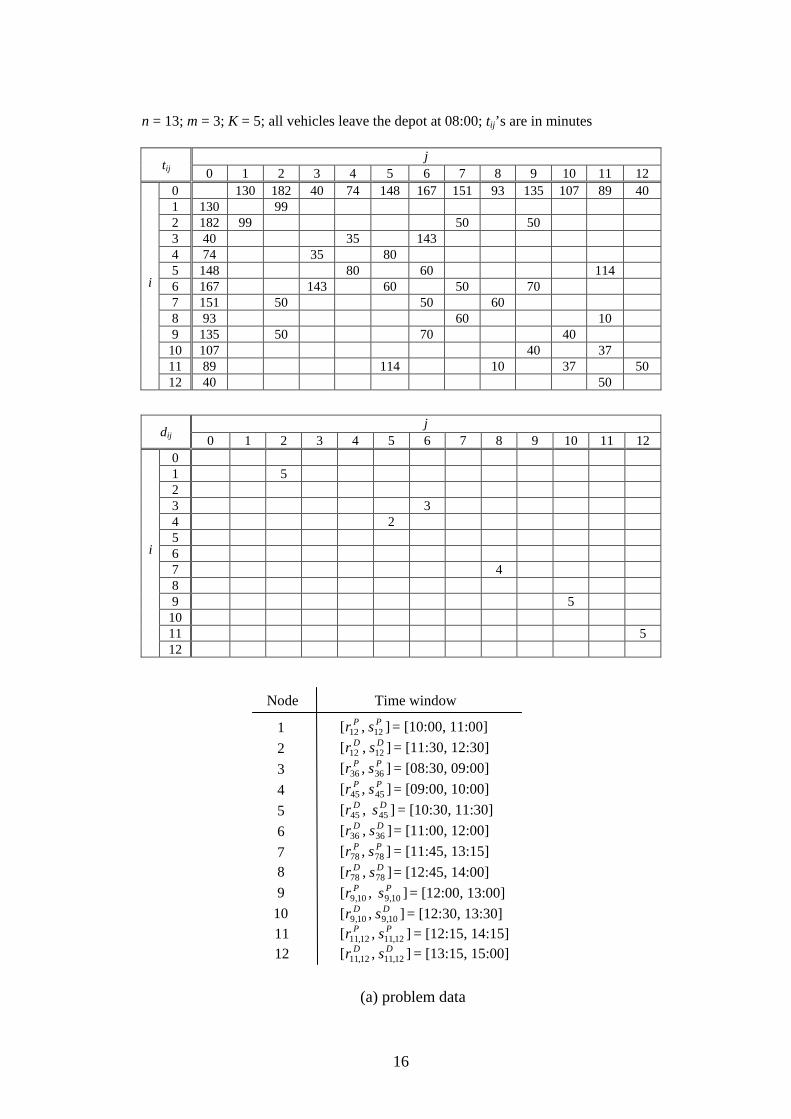
(a) problem data

n = 13; m = 3; K = 5; all vehicles leave the depot at 08:00; tij’s are in minutes

Node Time window

1 2 3 4 5 6 7 8 9

10

],[ 1212PP sr = [10:00, 11:00]

],[ 1212DD sr = [11:30, 12:30]

],[ 3636PP sr = [08:30, 09:00]

],[ 4545PP sr = [09:00, 10:00]

],[ 4545DD sr = [10:30, 11:30] ],[ 3636

DD sr = [11:00, 12:00] ],[ 7878

PP sr = [11:45, 13:15] ],[ 7878

DD sr = [12:45, 14:00] ],[ 10,910,9

PP sr = [12:00, 13:00] ],[ 10,910,9

DD sr = [12:30, 13:30] 11 12

],[ 12,1112,11PP sr = [12:15, 14:15]

],[ 12,1112,11DD sr = [13:15, 15:00]

17

(b) crossover operations

(c) corresponding chromosomes and fitness values

Figure 2: A numerical example

Parents:

Offspring:

C: )}2,12,11(),1,10,9(),2,8,7(),2,5,4(),2,6,3(),1,2,1{(

D: )}3,12,11(),2,10,9(),1,8,7(),3,5,4(),2,6,3(),1,2,1{(

A: )}2,12,11(),2,10,9(),1,8,7(),2,5,4(),2,6,3(),1,2,1{(

B: )}3,12,11(),1,10,9(),2,8,7(),3,5,4(),2,6,3(),1,2,1{(

4th entry 5th entry

route 1: 0 1 2 9 10 0 route 2: 0 3 4 5 6 7 8 11 12 0 fitness value = 426 + 425 = 851 route 1: 0 1 2 7 8 0 route 2: 0 3 6 9 10 0 route 3: 0 4 5 11 12 0 fitness value = 432 + 400 + 358 = 1190

route 1: 0 1 2 7 8 0 route 2: 0 3 4 5 6 9 10 11 12 0 fitness value = 432 + 452 = 884 route 1: 0 1 2 9 10 0 route 2: 0 3 6 7 8 0 route 3: 0 4 5 11 12 0 fitness value = 426 + 386 + 358 = 1170

4th entry 5th entry

18

Figure 3. Convergence of heuristic solutions

150

160

170

180

190

0 30 60 90 120 150 180 210 240

Running time (seconds)

Tota

l tra

vel t

ime

19

Table 1. Computational results 2=λ 4=λ 6=λ

50=n , 15=K R = 4.49% R = 1.30% R = 0.57% 50=n , 20=K R =10.08% R =11.00% R = 2.00% 50=n , 30=K R =12.90% R =11.80% R = 6.10% 100=n , 15=K R = 5.85% R = 5.15% R = 3.28% 100=n , 20=K R =11.00% R = 9.20% R = 1.97% 100=n , 30=K R = 5.99% R = 1.79% R = 3.45% 200=n , 15=K R = 1.75% R = 1.36% R = 3.60% 200=n , 20=K R = 0.50% R = 2.60% R = 1.01% 200=n , 30=K R = 5.38% R = 4.49% R = 0.57% 400=n , 15=K R = 0.64% R = 0.36% R = 0.08% 400=n , 20=K R = 0.05% R = 0.03% R = 0.20% 400=n , 30=K R = 0.62% R = 0.59% R = 2.93%

]45:1315:12[][ PP sr

A DYNAMIC ROUTING MODEL

Documents

Transcript of A DYNAMIC ROUTING MODEL