A Dynamic Optimization Framework with Model Predictive ...
88
A Dynamic Optimization Framework with Model Predictive Control Elements for Long Term Planning of Capacity Investments in a District Energy System Jose L. Mojica A thesis submitted to the faculty of Brigham Young University in partial fulfillment of the requirements for the degree of Master of Science John D. Hedengren, Chair Larry L. Baxter Vincent Wilding Department of Chemical Engineering Brigham Young University December 2013 Copyright © 2013 Jose L. Mojica All Rights Reserved
Transcript of A Dynamic Optimization Framework with Model Predictive ...
A Dynamic Optimization Framework with Model Predictive Control Elements for Long Term
Planning of Capacity Investments in a District Energy System
Jose L. Mojica
A thesis submitted to the faculty ofBrigham Young University
in partial fulfillment of the requirements for the degree of
Master of Science
John D. Hedengren, ChairLarry L. BaxterVincent Wilding
Department of Chemical Engineering
Brigham Young University
December 2013
Copyright © 2013 Jose L. Mojica
All Rights Reserved

ABSTRACT
A Dynamic Optimization Framework with Model Predictive Control Elements for Long TermPlanning of Capacity Investments in a District Energy System
Jose L. MojicaDepartment of Chemical Engineering, BYU
Master of Science
The capacity expansion of a district heating system is studied with the objective of evalu-ating the investment decision timing and type of capacity expansion. District energy is an energygeneration systems that provides energy, such as heat and electricity, generated at central locationsand distributed to the surrounding area. The study develops an optimization framework to findthe optimal investment schedule over a 30 year horizon with the options of investing in traditionalheating sources (boilers) or a next-generation combined heat and power (CHP) plant that can pro-vide heat and electricity. In district energy systems, the investment decision on the capacity andtype of system is dependent on demand-side requirements, energy prices, and environmental costs.The main contribution of this work is to formulate the capacity planning over a time horizon asa dynamic optimal control problem. In this way, an initial system configuration can be modifiedby a "controller" that optimally applies control actions that drive the system from an initial stateto an optimal state. The optimal control is a model predictive control (MPC) formulation that notonly provides the timing and size of the capacity investment, but also guidance on the mode ofoperation that meets optimal economic objectives with the given capacity.
Keywords: heating, network, capacity, expansion, boilers, energy, controller, optimal, timing, for-mulation, economic, dependent

ACKNOWLEDGMENTS
I would like to thank all the people involved who helped me with this project, especially
my advisor Dr. John D. Hedengren. Without his encouragement and support, I would not have
been able to grow and reach the capacity I have thus far. I am very grateful for the opportunities
he has given me to present and attend conferences as well as mentoring opportunities with other
group members and fellow students. These experiences enabled me to communicate and further
learn and develop my work. The original motivation for this project came from the work of Kody
Powell Ph.D. from the University of Texas at Austin. He has been a great collaborator and men-
tor throughout the project. In addition, the University of Texas Utility and Energy Management
contributed without hesitation with data resources. Reza Asgharzadeh has been a great help in the
development of this project. His forward thinking and collaborative attitude have been invaluable
many times to move this project forward, but most importantly his kind, supportive friendship. Da-
mon Petersen and Michelle Chen have both been great contributors, especially in preparing quality
data and modeling. I also want to recognize the incredible help from Abinash Paudel in assisting
with the formatting and final production of this document. Lastly, a special thanks to Brigham
Young University Physical Facilities and heating plant for their invaluable contributions to data
resources and knowledge.

TABLE OF CONTENTS
LIST OF TABLES . . . . . . . . . . . . . . . . . . . . . . . . . . . . . . . . . . . . . . . vi
LIST OF FIGURES . . . . . . . . . . . . . . . . . . . . . . . . . . . . . . . . . . . . . . vii
Chapter 1 Introduction . . . . . . . . . . . . . . . . . . . . . . . . . . . . . . . . . . . 1
Chapter 2 Background . . . . . . . . . . . . . . . . . . . . . . . . . . . . . . . . . . . 3
2.1 District Energy Systems and Combined Heat and Power . . . . . . . . . . . . . . . 3
2.1.1 Energy Systems Optimization Under Uncertainty . . . . . . . . . . . . . . 6
2.1.2 Dynamic Optimization and Model Predictive Control for Capacity Planning 9
2.1.3 Multi-objective Optimization in MINLP Framework . . . . . . . . . . . . 11
Chapter 3 Modeling District Heating system and CHP . . . . . . . . . . . . . . . . . 13
3.1 Modeling for Optimization . . . . . . . . . . . . . . . . . . . . . . . . . . . . . . 13
3.2 Modeling Boilers and CHP Elements . . . . . . . . . . . . . . . . . . . . . . . . . 14
3.3 From District Heating to CHP System . . . . . . . . . . . . . . . . . . . . . . . . 15
3.4 Traditional Capacity Expansion Models . . . . . . . . . . . . . . . . . . . . . . . 17
3.5 Simplified Demand Profiles . . . . . . . . . . . . . . . . . . . . . . . . . . . . . . 19
3.6 Discrete Linear Energy System Model . . . . . . . . . . . . . . . . . . . . . . . . 21
3.7 Dynamic Energy System . . . . . . . . . . . . . . . . . . . . . . . . . . . . . . . 22
3.7.1 Generating a Dynamic Energy Demand Horizon . . . . . . . . . . . . . . 22
3.7.2 Economic Horizon and Environmental Costs . . . . . . . . . . . . . . . . 25
3.7.3 Financial Indicators to Guide Capital Investment . . . . . . . . . . . . . . 27
3.7.4 Capital Investment Costs . . . . . . . . . . . . . . . . . . . . . . . . . . . 28
3.8 Dynamic and MPC Optimization Framework . . . . . . . . . . . . . . . . . . . . 28
3.8.1 Non-linear Dynamic Modeling . . . . . . . . . . . . . . . . . . . . . . . . 29
3.8.2 Numerical Solution of DAE Systems . . . . . . . . . . . . . . . . . . . . 29
3.8.3 MPC Formulation . . . . . . . . . . . . . . . . . . . . . . . . . . . . . . 30
3.9 Dynamic Model of CHP System . . . . . . . . . . . . . . . . . . . . . . . . . . . 32
iv

3.10 Uncertainty in Natural Gas and Electricity Prices . . . . . . . . . . . . . . . . . . 41
Chapter 4 Optimization Results and Discussion . . . . . . . . . . . . . . . . . . . . . 45
4.1 MPC Formulations Results . . . . . . . . . . . . . . . . . . . . . . . . . . . . . . 45
4.2 Utilization of Capacity . . . . . . . . . . . . . . . . . . . . . . . . . . . . . . . . 48
4.3 Optimization Under Different Economic Scenarios . . . . . . . . . . . . . . . . . 53
4.3.1 Economic Scenarios Relaxed Problem Results . . . . . . . . . . . . . . . 53
4.3.2 Economic Scenarios MINLP Results . . . . . . . . . . . . . . . . . . . . 55
Chapter 5 Conclusion and Future Considerations . . . . . . . . . . . . . . . . . . . . 58
REFERENCES . . . . . . . . . . . . . . . . . . . . . . . . . . . . . . . . . . . . . . . . . 61
Appendix A Dynamic Boiler Model . . . . . . . . . . . . . . . . . . . . . . . . . . . . . 65
Appendix B Energy System Dynamic Model . . . . . . . . . . . . . . . . . . . . . . . . 70
Appendix C CHP Correlations . . . . . . . . . . . . . . . . . . . . . . . . . . . . . . . 78
v

LIST OF TABLES
4.1 Results for three different MPC formulations for the expected energy prices eco-nomic case. . . . . . . . . . . . . . . . . . . . . . . . . . . . . . . . . . . . . . . 47
vi

LIST OF FIGURES
2.1 Generalized Schematic of District Energy System of an university campus. (cour-tesy Kody Powell Ph.D., UT Austin). . . . . . . . . . . . . . . . . . . . . . . . . . 4
2.2 Typical Combined Heat and Power System with HRSG [11]. . . . . . . . . . . . . 5
2.3 CHP versus Separate Heat and Power Production [9]. . . . . . . . . . . . . . . . . 5
2.4 MPC approach. ySP is the target set point of the system (i.e. energy demandtarget or emissions target). Tnt number of prediction horizon intervals, and Tnu isthe number of control horizon intervals. yi are the values of the output controlledvariables obtained by applying input manipulated variables ui [25]. . . . . . . . . . 10
3.1 Schematic of district heating system with boiler for heating only. . . . . . . . . . 16
3.2 Schematic of district energy system with CHP and backup boiler. . . . . . . . . . 17
3.3 Sample heating and electric load profiles for a particular summer 24 hour periodshowing the mismatch in heating and electric load peaks. . . . . . . . . . . . . . . 18
3.4 Schematic A show the discretization of actual demand profile represented by thesolid curve. B shows the rearangement to make a cumulative load curve. C showsthe reduction to base and peak load period. . . . . . . . . . . . . . . . . . . . . . 20
3.5 Sample electricity load profiles for a representative year (top) and week (bottom). . 24
3.6 Generated electricity and heating demand profiles for dynamic optimization. Eachcycle (trough to trough) represents an average day. There are 15 cycles becauseeach represents two years of constant demand for an average winter and summerday. . . . . . . . . . . . . . . . . . . . . . . . . . . . . . . . . . . . . . . . . . . 25
3.7 28 U.S. EIA commercial natural gas and electricity price forecasts [37]. . . . . . . 26
3.8 Probability distributions for natural gas prices. Each PDF curve denotes a differentprice distribution for a particular year in the time horizon. The distributions areused to calculate the CDF and then the expected natural gas prices at each point ofthe horizon through Equation 3.31. The same approach is used to find the expectedelectricity prices. . . . . . . . . . . . . . . . . . . . . . . . . . . . . . . . . . . . 44
4.1 CHP and boiler capacity investment plan from MPC formulation based on threedifferent control objectives for the expected energy prices economic case. . . . . . 49
4.2 Surplus heat profiles for the different MPC cases. MPC Case 3 has the lowestexcess heat for both winter and summer. For winter profile it goes to zero for MPCCase 3. . . . . . . . . . . . . . . . . . . . . . . . . . . . . . . . . . . . . . . . . 50
4.3 Heating supply profiles for MPC case 1 . . . . . . . . . . . . . . . . . . . . . . . 52
4.4 CHP capacity schedule based on different economic cases for relaxed problemformulation. . . . . . . . . . . . . . . . . . . . . . . . . . . . . . . . . . . . . . 54
vii

4.5 Boiler capacity schedule based on different economic cases for relaxed problemformulation. . . . . . . . . . . . . . . . . . . . . . . . . . . . . . . . . . . . . . . 55
4.6 CHP and boiler maximum capacities by economic scenario. . . . . . . . . . . . . 56
4.7 CHP capacity histogram (top) and boiler total capacity histogram (bottom). . . . . 57
C.1 Data and polynomial from [11] for CHP heat supply Equation 3.13. . . . . . . . . 78
C.2 Data and polynomial from [11] for CHP natural gas consumption Equation 3.19. . 78
C.3 Data and polynomial from [9] for CHP capital cost Equation 3.24 . . . . . . . . . 79
C.4 Data and polynomial from [52] for boiler capital cost Equation 3.25. . . . . . . . . 79
viii

Jose L. Mojica
December 13, 2013
CHAPTER 1. INTRODUCTION
Private and public utilities are confronted with a number of investment options to supply
their growing energy demands; investment in new energy systems must compete with other op-
portunities to improve the financial bottom line of the overall business or institution’s goals [1] .
Stakeholders want the answers to four fundamental questions for the success of the investment:
How much will be earned and when, and how much to spend and when? In the power generation
sector, uncertainty on type, timing and stringency of potential air emission regulations coupled
with uncertainties on fuel prices, future costs, and energy demand inhibit stakeholders from mak-
ing robust investment decision early on [2, 3]. Power producers also face the task of balancing
the opposite objectives of economic viability, security of supply, and environmental regulations.
These uncertainties and conflicting objectives that stakeholders face may cause them to make sub-
optimal decisions that delay investments. These suboptimal investments are are usually done in
small increments that in the long term can cost more than if a less uncertain investment option is
taken early on. In like manner, end users of energy like commercial and institutional facilities that
have a large energy demand from buildings also face similar challenges as they try to fulfill their
growing energy needs and simultaneously comply with pressures to reduce their carbon footprint.
One example of those regulations come from EPA Title V of the Clean Air Act, an air operating
permitting program that applies to major emitters of air pollution and some other non-major source
producers [4]. Title V regulations can affect non industrial institutions like hospitals, universities,
or research campuses that produce their own energy for mainly space heating and cooling such
as on-site heating plants. In large building campuses, energy demand is usually supplied through
a combination of heating plants and electricity from the grid. To face those conflicting objec-
tives, a growing number of institutions are turning to more energy efficient combined heat and
power (CHP) plants to meet energy demands. When an on-site CHP system is properly planned,
1
designed, constructed, and operated, it offers a proven method to lower overall facility energy
consumption and costs, and reduces total overall utility system fuel consumption [5].
Incorporating a CHP system may be a good alternative in leveraging the uncertainties from
the economic and environmental forces to the growing energy demands of the institution. But
in considering such investment, the institution must decide on numerous options like whether to
continue expanding traditional combustion units for heating plants, installing pollution abatement
equipment, reconfiguring the entire space heating/cooling system to an electricity only system,
adding energy storage capabilities, or rather to build a new CHP unit that may reduce the costs
associated with future CO2 emissions [3]. With so many options and an uncertain outlook on fuel
costs, demand, and regulations; there is a motivation to optimize the investment and operations
decisions for these types of problems to ensure reasonable return on the investment [6]. An op-
timization approach to solve such problems has been attempted in the past decades that mainly
focuses on characterizing uncertainty in model parameters and key inputs under a linear model
framework. A holistic optimization approach that takes into account multi-objective issues under
uncertainty, system dynamics, and intrinsic non-linear constraints is yet to be fully developed for
capacity expansion and investment planning problems. This work introduces a dynamic multi-
objective optimization approach based on a Model Predictive Control (MPC) framework to find
an optimal long-term planning horizon decision outlook for the capacity of a future CHP plant
to answer the pressing questions timing and capacity of investment. The optimization framework
is applied to an university campus energy system, but the goal of this work is to provide the
optimization methods and modeling knowledge to other energy systems with dynamics, system
uncertainties, and nonlinear constraints that affect the capacity planning over a time horizon.
2

CHAPTER 2. BACKGROUND
2.1 District Energy Systems and Combined Heat and Power
District energy systems are energy generation systems that provide any combination of
electrical distribution, heating, and cooling, where heating and cooling are generated at central
locations and distributed to the surrounding area. District energy systems take advantage of
economies of scale to efficiently and cost-effectively provide heating, cooling, or electricity for
an immediate surrounding area. Buildings can be supplied by large centrally-located generation
equipment, rather than smaller individual units for each building [7]. District energy systems can
be composed of various energy conversion technologies such as traditional gas or coal boilers,
reciprocating engines, combustion turbines, or industrial processes that generate excess heat. In
addition to the energy conversion technology available, the district energy system may include ther-
mal energy storage to offset demand constraints when thermal energy is not sufficiently available
or shift production to times of the day when it is more cost effective to produce energy. Regardless
of the components that constitute the district energy system, the overall effectiveness of the energy
systems heavily relies on how the components of the energy systems interact with each other [8].
The interaction of the system components will depend on the energy demand, system constraints,
and system dynamics.
One of the most efficient district energy system arrangements is that of a combined heat
and power (CHP) plant, also known as a cogeneration plant. A CHP plant simultaneously produces
heat and generates power from a single fuel source [5]. CHP systems can consist of a number of
individual components like the prime mover, generator, heat recovery, and electrical interconnec-
tion. The prime mover is the type of equipment that drives the overall system and it will typically
identify the CHP system. Prime movers for CHP systems include reciprocating engines, combus-
tion or gas turbines, steam turbines, microturbines, and fuel cells. These prime movers are capable
3

Figure 2.1: Generalized Schematic of District Energy System of an university campus. (courtesyKody Powell Ph.D., UT Austin).
of burning a variety of fuels, including natural gas, coal, oil, and alternative fuels to produce shaft
power or mechanical energy [9].
In building campuses where electric loads are larger than 1 MW, combustion turbine gen-
erators (CTG) are popular prime movers for CHP considerations. A combustion turbine system
mainly consists of compressor, combustor, and turbine. CTG are commercially available in many
capacities varying from small 1 MW to 100 MW utility scale generators [5]. Martens et al. in
a survey of CHP efficiencies reports that small gas turbines (<10 MWe) have electric efficiencies
lower than 30%, whereas gas turbine based CHP systems between 10 and 40 MW reach electric
efficiencies of 30 to 40%. Gas turbines larger than 40 MW have electric efficiencies of about
35% [10]. The remaining energy from the combustion is discarded in the exhaust where it is then
recovered by a heat recovery boiler. A heat recovery boiler is similar to a typical fuel fired boiler
but instead of using the heat from a separate combustion reaction, the exhaust from the turbine is
the source of heat to make hot water or steam depending on the need of the overall district energy
system [5]. When the heat recovery boiler produces steam, it is called a heat recovery steam gen-
erator (HRSG). If the energy from the exhaust gas from the turbine is not enough to supply the
heating needs of the system, supplemental burners and or extra boilers in parallel maybe needed
4

Figure 2.2: Typical Combined Heat and Power System with HRSG [11].
Figure 2.3: CHP versus Separate Heat and Power Production [9].
to supplement the heat recovery boiler. The heat recovery part of the system will have efficien-
cies of traditional boilers of around 80%. Although operating conditions and capacity size have
significant effects on the overall efficiency of a CHP system, the combined processes of power
generation and subsequent heat recovery as illustrated in Figure 2.2 have expected efficiencies of
around 75 percent [10]. Conventional generation to provide electric power and heat separately will
have expected efficiencies of less than 50 percent as illustrated in Figure 2.3 where it compares
conventional generation and a CHP option using a natural gas combustion turbine [9].
5

District energy systems also extend the opportunities for optimization beyond electrical
generation and distribution, creating the opportunity for a smart and diverse energy network which
provides energy for electrical, heating, and cooling demands [7]. While there is more opportunity
for optimization in these systems, the optimization problems themselves are more complex and
require models of a diverse range of systems. They also have additional constraints which must
be adhered to, including simultaneously meeting other (non-electrical) loads, such as heating and
cooling [7]. While optimization methods have been used to exploit savings in energy and reduc-
tion of operating costs in operating district CHP systems, the same considerations have not been
extended to planning of capacity of district energy systems.
2.1.1 Energy Systems Optimization Under Uncertainty
Decision making in many industries inherently involves consideration of multiple objec-
tives and uncertain outcomes; and in many situations, we must make decisions at different times
and at different levels. Those types of problems are generally referred as multi-objective decision
processes under uncertainty [12].
Investment and planning decisions in power generation systems fit the above description.
As power generation systems become larger and more complex, the number of possible system
configurations and technologies that could possibly meet the designer’s objectives in an optimal
manner increases greatly [13]. The added level of complexity in energy systems usually comes
in the form of more efficient and novel equipment because of motivations to conserve energy
resources due to economic and geo-political justifications and greater efforts in reducing green
house gasses that are increasingly tied to rising global temperatures. In addition, the system may
need to be developed taking into account both the dynamic, economic, and environmental effects
on system performance. Thus, the difficulty of developing the entire system via the formulation
of a single optimization problem is great due to the complexities involved. These complexities are
further heightened with the introduction of uncertainty analysis into the problem, transforming the
problem from a purely deterministic one into a probabilistic one [13].
Subramanyan et al. [14] describes that in the design of a power system there are three basic
types of uncertainties that must be taken into account:
6

1.) Uncertainty with respect to the model parameters: These parameters are a part of the
deterministic model and not actually subject to randomness. Theoretically their value is an exact
number. The uncertainty results from the impossibility of exactly modeling the physical behavior
of the system.
2.) Uncertainty in the input variables: This kind of uncertainty originates from the random
nature and unpredictability of certain process inputs.
3.) Uncertainty in the initial conditions: These types of uncertainties result due to the
complications in predicting the initial conditions of the operation.
In a capacity expansion or investment planning optimization problem, such as the one pre-
sented here, it may only be necessary to focus on the uncertainty with respect to the model param-
eters and that of the input variables and disturbances. It can be assumed there is little uncertainty
in initial conditions because the status quo of the system is known.
In the past decades the majority of the methods dealing with uncertainties for power gen-
eration systems are related to stochastic mathematical programming [15]. More specifically, op-
erations researchers have developed two main types of solution methods: multi-stage stochastic
programming (MSSP), and stochastic optimal control (SOC). A notable number of studies that ap-
proach the problem of power generation system capacity expansion and investment planning under
uncertainty have been developed as MSSP problems [2, 13, 16]. SOC solution approaches are also
found for similar problems but in much less frequency [17].
MSSP more specifically deals with problems that involve a sequence of decisions reacting
to outcomes that evolve over time. At each stage a decision is made based on currently available
information [12]. In many problems where random variables follow multi-dimensional continuous
distributions it becomes very difficult to numerically solve those problem because it requires mul-
tivariate integration. To avoid this problem, sampling or discrete approximation of the distributions
is done to represent the probable space. Those scenarios are many times modeled as a scenario
tree that represent discrete scenarios to satisfy specified statistical properties [12]. When a scenario
tree is specified, the stochastic program becomes a deterministic equivalent program that is easier
to solve [18]. Although this approach makes the problems much more tractable, it stills begs the
question of how well the scenario tree actually describes the uncertainty in the variables. Defin-
7

ing a suitable scenario tree is a challenge by itself and still special numerical techniques based on
decomposition, aggregation and parallelization are required to solve large-scale problems [12].
SOC can also be referred as Markov decision process, in which the algorithm searches for
optimal actions to take at generally discrete points in time in the state being occupied [18]. The
actions are taken based on predefined decision rules or policies which are influenced by random
outcomes at each specific state and stage [12, 18]. In this fashion, the solution approach is to
form a backward recursion that results in an optimal decision associated with each state and each
stage [18]. Both MSSP and SOC suffer from the “curse of dimensionality,” but in different ways: in
MSSP because of the large sample space, and in SOC because of the immense state space [12,19].
There are certain criteria that are useful in explaining whether a MSSP approach or a SOC
approach should be employed. MSSP approaches are reported to be more suitable for solving long-
term strategic planning problems, such as capacity planning that have relatively small number
of periods and scenarios [12]. SOC problems are reported to work better in problems such as
production and inventory control where there are relatively many periods and scenarios but a state
space of modest size [12]. This explains the greater use in the literature of MSSP versus SOC for
energy systems infrastructure planning under uncertainty. Although the approach to the solution by
the two methods is different, Cheng et al. demonstrated that the two methodologies are equivalent
in that the decision policy prescribed by SOC is the same as the corresponding optimal decision
found by MSSP [12].
In a similar problem of investment and planning for power generation systems under un-
certainty Fuss et al. used a real options valuation approach to find a solution [19]. They reported
that a MSSP or SOC approach would have resulted in the same outcomes as those obtained in a
real options approach. Their work also reports that the main reason for not using stochastic meth-
ods was the increased computational intensity due to the dimensionality explosion when there are
many periods and scenarios, as well as a modest state space [19].
Other less common, but reported methods in the literature to account for uncertainty in
power generation systems expansion and investment planning problems include fuzzy logic [20]
and Monte Carlo simulations [21]. Others have used a combination of methods to account for
uncertainty. For example, joint probabilistic programming and fuzzy possibility programming was
used by Lou et al. in an optimization approach for power generation planning under uncertainty
8

in a mixed integer linear programming (MILP) framework [15]. Another combined method to
account for uncertainty was recently reported by Y.F. Li et al. in which a MSSP and fuzzy linear
programming is introduced into a MILP framework [22]. Li et al. report that the benefits of
such formulations lies in that their approach can tackle uncertainties described in terms of interval
values, fuzzy sets, and probability distributions [22]. In energy system planning under uncertainty,
the combined method approach can reflect dynamic decisions for facility-capacity expansions and
energy supply over a multistage context [22].
2.1.2 Dynamic Optimization and Model Predictive Control for Capacity Planning
Dynamic Optimization constitutes a methodology to optimize systems represented by dy-
namic models in the form of differential and algebraic equations (DEA). The optimization algo-
rithms for dynamic optimization may handle nonlinear objective functions and constraints with
continuous or integer variables. Dynamic optimization is an integral part of some advanced con-
trol algorithms such as Model Predictive Control (MPC). MPC is an important advanced control
technique that utilizes explicit process models to predict future response of a plant or system [23].
The process models used in MPC are in many cases dynamic and non-linear and capture the dy-
namic and static interactions between inputs, outputs, and disturbances affecting the system [24].
In control applications of complex chemical and energy processes, MPC technology is extremely
beneficial because the algorithms attempt to optimize not only the present optimal control moves,
but also optimize future system behavior by computing a sequence of future decision variables ad-
justments [23]. MPC’s ability to predict future variable moves through optimization has similarities
to the objectives of capacity planning over a future horizon where economic, environmental, and
operational targets must be achieved while the capacity of the system must be optimally planned
out under the constraints and uncertainty of the system.
Ricardez-Sandoval et al. [26] reviewed different approaches to simultaneously design and
control large systems under process parameter uncertainty. Large systems such as chemical plants
are usually designed based on steady state economic calculations, while the control aspects are
studied independently. The sequential fashion of the approach from design and control give rise to
unforeseen constraints and limitations that can greatly hinder the economic operation of the system
once online. The simultaneous optimization of dynamic control variables and design variables
9

Figure 2.4: MPC approach. ySP is the target set point of the system (i.e. energy demand targetor emissions target). Tnt number of prediction horizon intervals, and Tnu is the number of controlhorizon intervals. yi are the values of the output controlled variables obtained by applying inputmanipulated variables ui [25].
can thus greatly reduce the effect of under sizing or over sizing the capacity of the system and
improved profitable operation under different market conditions [26]. From an uncertainty point
of view, the dynamic behavior of system parameters and variables is a factor that must addressed in
power systems optimization [14], thus the explicit inclusion of system dynamics in the optimization
problem as proposed in this work should have a measurable reduction of uncertainty on the optimal
size of the system.
From the previous section on stochastic optimization approaches, there is a lack of literature
that reports on optimization frameworks that use system dynamics for capacity planning of energy
systems. One reason can be attributed to the curse of dimensionality limits found in stochastic pro-
gramming approaches. System dynamics in the formulation of the problem adds complexity and
enlarges the problem, making it even more difficult to solve with current optimization technology.
Another reason could be attributed to the recursive features of stochastic programming which do
not lend itself to a dynamic model form. The motivation to include system dynamics to optimize
capacity planning of energy systems comes from practical experience reported in already planned
and constructed plants in which owners find that the planned capacity is not being fully utilized,
10

not enough, or no longer cost effective given changing economic conditions and the load following
requirements of the system [27].
2.1.3 Multi-objective Optimization in MINLP Framework
Although the MSSP and SOC approaches historically have been able to provide solutions to
planning and scheduling problems under uncertainty, computational expense is one serious draw-
back. When multi-objective options are incorporated in the MSSP problems, solution times even
in the order of days are not uncommon for relatively modest size problems [12]. Science and en-
gineering problems normally feature several and contradictory design and or operation objectives
that can be benefited from using new and integrated ways of solving such problems [28]. One
innovation is solving these types of problems as a multi-objective, mixed integer programming
formulation.
Antunes et al. [29] reports on a multiple objective mixed integer linear programming (MOMILP)
model for power generation expansion planning. One important contribution is the consideration
of modular expansion capacity values. This approach avoids the need to discretize results in a post-
processing phase. In addition their MOMILP approach also focuses on an interactive algorithm
that provides decision support in the selection of satisfactory compromise designs (Pareto front
designs) [29]. This is an important matter to consider because it can help identify in a systematic
way the potential compromised solutions that otherwise can be ignored.
Whether the method to account for uncertainty is a stochastic, fuzzy, Monte-Carlo, or a
combination of more than one, the most common optimization framework reported in the litera-
ture is the MILP approach. The disadvantage in a MILP approach lies in cases where the sys-
tem contains non-linear and non-convex constraints in which suboptimal solutions can arise when
solved with methods that assume convexity [6]. The application of a mixed integer non-linear
programming (MINLP) approach has the potential of providing better results when encountering
non-linearity and non-convexity as it is presented in this research.
Gupta and Grossmann in a recent conference proceeding [6] demonstrated the use of
MINLP for optimal development planning of offshore oil and gas fields with complex fiscal rules
and under nonlinear and non-convex features. Although their approach falls short of a multi-
11

objective application, Gutierrez-Limon et al. expand the application of MINLP alongside a multi-
objective optimization approach for scheduling and control for a class of chemical reactors [30].
Historically multi-objective problems in MINLP frameworks have been solved by using a
single objective function that is subject to different weights. Those weights are subjective and can
give misleading or suboptimal results [25]. On the other hand, multi-objective optimization gives
rise to the Pareto front which enables the designer to assess the advantage/disadvantage of a given
optimal solution [28]. An advantage from this approach is that the results from the Pareto front
allow us to pick up an optimal point containing target behavior [28].
Multi-objective mixed integer non-linear programming (MO MINLP) approaches are the
latest advances in optimization techniques for problems suitable for this type of formulation. MO
MINLP is starting to be applied to scheduling and control problems in highly nonlinear chemical
processes [28]. The possibility exists of online applications in the form of MO MINLP model
predictive control as long as the computational times can be feasible for the online process [25].
But as demonstrated by Gupta and Grossman [6], MINLP can be applied to investment and infras-
tructure planning and a MO MINLP that simultaneously takes into account process uncertainty is
the technological frontier that must be further developed.
12

CHAPTER 3. MODELING DISTRICT HEATING SYSTEM AND CHP
3.1 Modeling for Optimization
A model is a mathematical description of a physical system. One class of mathematical
models is referred to as optimization models. Optimization algorithms search for a feasible design
according to specified criteria [31]. If the aim is to minimize cost and plan for optimum capacity of
a district energy system, the model must be able to calculate cost and represent the capacity with
mathematical equations that represent the energy output of the system. The economic and math-
ematical representation of the dynamics and physical system can be done through first principles
or empirical models. Modeling the system through first principles is usually more accurate and
intuitively descriptive because the equations will account for thermodynamic, mechanical, chem-
ical, transport phenomena, and any other pertinent fundamental science, but it takes the largest
amount of effort and system knowledge to accurately represent all aspects of the system with these
fundamentals. On the other hand, pure empirical models are easier to generate but require data
from the system being modeled which in many cases might be difficult to obtain at the range of
operating conditions desired. A combination of first principles and empirical modeling may be the
best option to leverage first principles system knowledge and available data. Parts of the system
may be too complex to mathematically represent and require an empirical model. In this work,
the mixed approach of first principles and empirical models was used to represent the CHP energy
system. This is necessary because the purpose of the optimization program is to find capacity and
timing of investment while at the same time responding to diurnal power and heat energy loads of
the system. Those goals do not require detailed operating conditions of the CHP system, but do
require dynamic response to energy load changes.
13

3.2 Modeling Boilers and CHP Elements
The motivation in planning for capacity improvements of a district energy system comes
from the fact that many district energy systems are district heating systems with an aging fleet of
coal and natural gas burning boilers. A district heating system only provides thermal heat from
local generation, while power is imported from the grid. The coal or gas boiler based district
heating system can be modified to next generation CHP systems that may include a gas turbine
and heat recovery boiler elements in the model.
Boiler Modeling
In preparation for this work, considerable efforts were made to understand the system dy-
namics of the boilers which provide the main heating source for a building campus district energy
system. The first step was to generate a model that could represent the cycling time and tempera-
ture changes of a coal-fired furnace. The model was created using first principles based on material
and energy balances. The energy balance was built around the boiler, with appropriate heat-transfer
terms for exchange between the bed, tubes, and high temperature water. A heat transfer term was
incorporated into the model to represent the time delay of heating up and cooling down. The heat
transfer was based on irradiative heating, as this is the dominant form of heating certain types of
coal-fired boilers (Basu, Kefa, Jestin, 2000).
A second step in making the boiler model more representative of an operating system was
the inclusion of nonlinear dynamic equations that represent the dynamics of the steam drum in
a boiler. In operating district energy systems where steam is generated to provide heating and
or power for turbines, the main operating goal is to control the steam drum pressure. Since the
steam turbines and steam network for heating operate at target pressures, dramatic load changes or
sudden upsets in the steam network can upset the pressure and water level of the steam drum with
dangerous consequences such as drying or over flowing the drum. Poor drum water level control
has been reported to cause up to 30 % of emergency shut downs in utility scale boilers [32].
From the extensive and widely cited work of Alstöm et. al. in modeling boiler dynamics
[32], model drum pressure equations were used to simulate boiler load following. Although this
dynamic boiler model is not used in the capacity planning problem, the initial effort to model and
14

simulate control of boilers provides fundamental understanding of the interaction and limitations
a district energy system has in meeting energy demands. See Appendix A for full dynamic boiler
model.
Gas Turbine
The models for the gas turbine generators can be developed using steady-state or dynamic
first principles models. The power generated by the gas turbine is a function of the air flow, the fuel
flow, the inlet temperature, the temperature at the exit of the compressor, the firing temperature,
and the exhaust temperature [7]. Although these factors are extremely important in optimizing
online control and interaction of the gas turbine to predict fast dynamics, in a capacity planning
problem only the relationship of fuel consumption and power generation are important to establish
capacity requirements. To establish a simulated dynamic response to power generation, a first-
order differential empirical equation may suffice along with other algebraic relationships for fuel
consumption fitted from manufacturer’s data.
3.3 From District Heating to CHP System
Figure 3.1 illustrates a typical university campus district energy system. In such arrange-
ment, the buildings and cooling system represent the heating and cooling loads. The heat is pro-
vided solely by coal-fired or gas-fired boilers while the electric power supply only comes from the
city’s electrical grid. The heat produced from the boilers is directly used to provide all the energy
for space heating during the winter months as well as any auxiliary uses such as kitchens, showers,
laboratories, etc. During the summer months, the boilers continue to operate to provide heat for
absorption chillers and auxiliary uses.
A conversion of the current district energy system to one that includes a CHP arrangement
is illustrated in Figure 3.2. The new arrangement adds a few important components:
• gas turbine with generator for electricity
• heat recovery boiler
• back-up boiler capacity
15

Figure 3.1: Schematic of district heating system with boiler for heating only.
The distribution of heat and electricity to the district energy system remains the same, thus making
it only necessary to upgrade the energy generation units and interconnections to the heating and
electrical network. This work seeks to answer how large the the CHP plant must be, in terms of
capacity, and when it should be installed. The CHP in this analysis will reference a gas turbine and
heat recovery boiler combination, while the boiler will refer to a stand-alone combustion chamber
that only provides heat.
One of the most important factors in the effectiveness of a CHP plant is how the system can
respond to diurnal energy loads. District energy systems can have heating and power loads that
match their diurnal and seasonal cycles, but in many cases they don’t. In a campus building system
during the winter months, heating loads usually peak in the morning times as buildings warm up
from the cooling effect of the night, and power peaks in the afternoon when building occupancy is
at a maximum and lighting, electronics, etc. are at peak use. During the summer months, heating
has a more leveled load, but the electrical load will be much larger. The mismatch between heating
and electric load profiles creates tradeoffs that facility owners evaluate and optimize in terms of
16

Figure 3.2: Schematic of district energy system with CHP and backup boiler.
the type of energy system that will match energy needs. Figure 3.3 shows energy profiles for the
system being studied for a particular summer 24 hour period.
3.4 Traditional Capacity Expansion Models
The design capacity of a power plant is the maximum amount of energy per unit time that it
can produce [33]. Typical values in the US are measured in MMBTU/hr (1 million BTU per hour)
for heat generating systems and in megawatts for medium-size electric power generation systems.
Most systems are oversized for typical load scenarios or may include multiple units that can be
staged on or off as demand changes.
Because of growing energy demands and regulations on existing energy production fleets,
new investments in design capacity must be considered to meet increases in energy demand and
compliance with regulations. At the same time, energy demand is uncertain because of weather
and economic factors. Capacity expansions projects are mostly considered irreversible investments
because of high capital cost and the plants remain available for an extended period of time. This
17

Figure 3.3: Sample heating and electric load profiles for a particular summer 24 hour period show-ing the mismatch in heating and electric load peaks.
makes the design capacity investment decision a nontrivial one. When the design capacity exceeds
demand, the overall capital cost is likely to be too high. Alternatively, when the capacity is insuf-
ficient, the plants can be expected to operate at peak capacity and extra supply must be imported
from an external grid. Both these events are generally costly in terms of either excess capital cost
or higher priced power from external sources.
As previously stated at the beginning of this chapter, the modeling approach of a system
will dictate the quality of information obtained from an optimization program. The level of com-
plexity such as the use of linear versus non linear equations, differential versus algebraic only,
etc. will also dictate the optimization method and algorithms available to solve those types of
problems. To name a few, these include linear programming (LP), quadratic programming (QP),
nonlinear programming (NLP), mixed integer linear programming (MILP), mixed integer nonlin-
ear programming (MINLP). Detailed explanations about these optimization methods can be found
in many references [31,34]. The field of operations research continually seeks to improve solution
methods to solve ever more complex and larger problems. From a historical perspective, linear
methods have been widely used because of their relatively simple modeling complexity and ease
18

of solving with available computer power. Newer non-linear methods that can now solve larger
models with larger amounts of data are the new frontier in optimization technology.
In the next two sections, the traditional modeling formulation approach based on linear
steady state model and LP optimization method is introduced with an effort to contrast the differ-
ences with the proposed dynamic non-linear optimization approach with differential and algebraic
equations (DEAs) to solve capacity planning problems. An innovation of this research is the direct
application of DEAs to simultaneously optimize operating strategy and long-term planning.
3.5 Simplified Demand Profiles
Electricity demand varies over days, weeks, seasons, and years. Rather than model demand
over extended periods of time, traditional power expansion studies only consider a representative
single time period of one day. This choice simplifies the model, but still allows for demand sce-
narios that typify demand throughout a planning horizon of years [33].
Further simplifications of the one day time period is usually done by first discretizing the
one day profile into 24 separate periods. Although some dynamic fidelity is lost, it roughly follows
the demand curve. Next the 24 separate periods are rearranged to create a cumulative load curve.
From the cumulative load curve peak and base load periods can be extracted to approximate the
maximum capacity and base capacity needed to supply the demand. Although this approach pro-
vides a good approximation of demand, the dynamic interaction between heat and electricity in a
CHP system is lost. In Figure 3.4 the energy load profile reduction process is illustrated.
19

Figure 3.4: Schematic A show the discretization of actual demand profile represented by the solidcurve. B shows the rearangement to make a cumulative load curve. C shows the reduction to baseand peak load period.
The simplification of the demand profiles to two periods, base and peak, greatly reduces
problem size when optimizing over a long term time horizon.
20

3.6 Discrete Linear Energy System Model
To contrast the novel contributions of this work, first a traditional linear power plant ca-
pacity planning problem from [33] was modified to a campus energy system to optimize capacity
planning with CHP and boiler options. This model does not have differential equations or higher
than first order algebraic equations. The traditional linear capacity expansion models depend on
discretization of time steps and indexation of equations to approximate demand load changes and
utilization of the capacity, but cannot model dynamic behavior of the system.
Indices :
p plant type {chp, boiler}
k demand category {base load, peak load}
s season {summer, winter}
i energy type {electric, thermal}
Parameters :
ep existing capacity of plant type p [MW ]
ccp daily fraction of capital cost of plant p [MW ]
ocp daily operating cost of plant p [USD/MWh].
ick,s electricity import cost [USD/MWh]
dk,s,i instantaneous energy demand [MW ]
duk,s,i duration of demand [hours]
rk,s,i required energy [MWh]
fhrg recovered heat factor [unitless]
where the parameter rk,s,i is defined as rk,s,i = (dk,s,i−dk−1,s,i) ·duk,s,i
Variables :
xp new design capacity of plant type p [MW ]
yp,k,s allocation of capacity to demand [MW ]
zk,s import of electricity [MW/h]
Minimize :
∑p
ccp(ep + xp)+∑k
∑s
ick,s · zk,s +∑k
∑s
∑i
duk,s,i ·
(∑p
ocp · yp,k,s
)(3.1)
21

Subject to :
ep + xp ≥∑k
∑s
yp,k,s f or all p (3.2)
rk,s,electric = zk,s +duk,s,electric ·
(∑p
ychp,k,s
)f or all k,s (3.3)
rk,s,thermal ≤ duk,s,electric ·
(∑p
yboiler,k,s + ychp,k,s · fhrg
)f or all k,s (3.4)
xp ≥ 0, yp,k,s ≥ 0, zk,s ≥ 0 (3.5)
The above linear model in general typifies the traditional optimization approaches for ca-
pacity planning expansion. The capacities denoted by xp are lumped variables that quantify capac-
ity without a realistic physical or dynamic representation of it. Linear models are also the basis
for stochastic programming formulations. The stochastic formulations explicitly take into account
probabilistic factors as discussed in the background section of this work, but they lack the intrinsic
dynamic features. Yet perhaps the greatest deficiency is the inability for the formulation to handle
differential and algebraic equations in continuous space to explicitly handle the differential and
algebraic relationships.
The next sections illustrate the novel approach of this work in formulating and solving ca-
pacity expansion planning problems. This novel approach considers the long-term capacity plan-
ning problem with seasonal and dynamic energy demand horizon while subsequent sections treat
costs associated with environmental, operational, and capital equipment expansions.
3.7 Dynamic Energy System
3.7.1 Generating a Dynamic Energy Demand Horizon
The diurnal energy profiles, as those illustrated in Figure 3.3, characterize the net energy
usage of the system. Over long periods of time the demand profile curves reflect the overall effects
weather, building occupancy, and growth have on energy consumption. Energy generation systems
22

must be able to handle these uncertainties and projected growth. Due to increasing energy demand
and tougher environmental standards, new capacity must be added or completely new systems
installed. Those options must be evaluated against a realistic projected energy demand over the
lifetime of the proposed system. From historical data, energy system owners can obtain seasonal
and diurnal energy demand data over many years to analyze the cyclical aspects of the demand,
and then make year over year growth projections. In institutions such as university campuses,
long-term energy consumption growth typically has a well defined projected target due to finite
student enrollment goals and building plans. Figure 3.5 shows the campus demand data over an
entire year which shows cyclical daily profiles, as well as weekly and seasonal patterns exhibited
by the system.
In this work, the entire energy profile of two years is analyzed and broken into two parts,
summer and winter. Separately for summer and winter parts, the individual 24 hour periods are
isolated and averaged over each hour. This process in return gives an average 24 hour energy
demand profile for winter and summer periods. With this approach the extreme demand cases that
the system encounters in any one year are lost in the averaging. To counter that deficiency, the most
extreme 24 hour episodes for each season are isolated and then averaged with the seasonal daily
demand average. This creates a representative 24 hour demand profile that represent most energy
demand cases. These procedures are repeated for both heating and electrical energy demands.
Upon finding the average demand curves, these are propagated over a 30 year horizon
with a stochastic linear growth of 2.5% to simulate year over year energy demand increase of
an university campus. Each 24 hour cycle represents a seasonal average day for that year. At
the end, the demand curves for every two years are averaged thus assuming that energy demand
stays constant every two years. Although these assumptions are far from actual conditions, it is a
method to reduce the number of time points the optimization must consider while at the same time
providing the diurnal demand profile that the energy system must adapt to. This method contains
more information and dynamic features than the lumped peak and base load periods of traditional
modeling methods.
Although diurnal and seasonal energy cycles as well as energy growth projections are un-
certain, the level of uncertainty is greatly diminished from the analysis of historical demand data
because better projections can be made for the future horizon. This enables stakeholders to fo-
23

Figu
re3.
5:Sa
mpl
eel
ectr
icity
load
profi
les
fora
repr
esen
tativ
eye
ar(t
op)a
ndw
eek
(bot
tom
).
24

Figure 3.6: Generated electricity and heating demand profiles for dynamic optimization. Eachcycle (trough to trough) represents an average day. There are 15 cycles because each representstwo years of constant demand for an average winter and summer day.
cus on other uncertain economic forces that have a greater effect on the profitability of energy
generation systems such as electricity and natural gas prices and environmental regulation costs.
3.7.2 Economic Horizon and Environmental Costs
Fossil fuel prices and increasing environmental and health-impact concerns have forced
decision makers to contemplate and propose comprehensive studies to evaluate energy systems
management [22]. A recent report from the European Union indicates that high investment costs,
long payback periods of irreversible investments in new power plants, commodity price variability
in deregulated power markets, and regulatory uncertainty bear significant risks for the investing
stakeholders [35]. Those concerns have already postponed or even canceled planned investments
in new fossil power plants [35]. In the United States, similar cost due to environmental based
regulations are hampering the growth in coal-based power production. For CHP systems which
still depend on fossil fuels, mainly natural gas, the outlook is more favorable due to the efficiency
increases and lower carbon footprint. The main driver in the recent economy for natural gas con-
suming processes comes from falling natural gas prices because of abundant natural gas resources
25
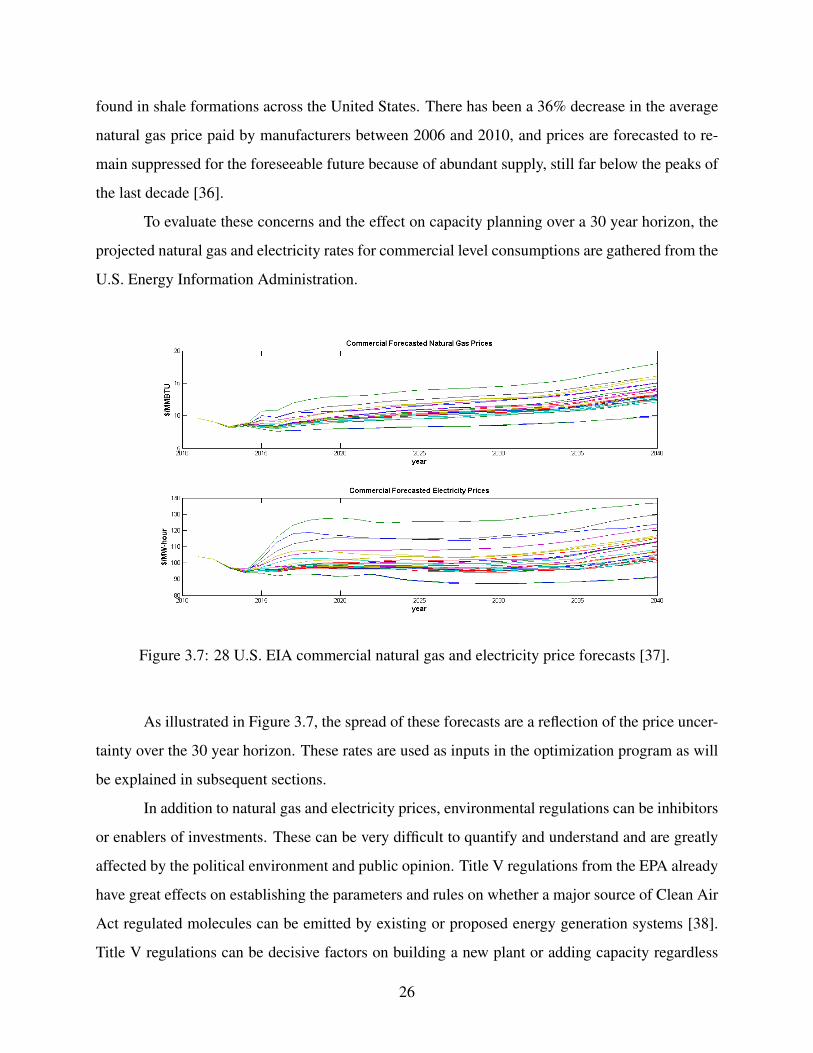
found in shale formations across the United States. There has been a 36% decrease in the average
natural gas price paid by manufacturers between 2006 and 2010, and prices are forecasted to re-
main suppressed for the foreseeable future because of abundant supply, still far below the peaks of
the last decade [36].
To evaluate these concerns and the effect on capacity planning over a 30 year horizon, the
projected natural gas and electricity rates for commercial level consumptions are gathered from the
U.S. Energy Information Administration.
Figure 3.7: 28 U.S. EIA commercial natural gas and electricity price forecasts [37].
As illustrated in Figure 3.7, the spread of these forecasts are a reflection of the price uncer-
tainty over the 30 year horizon. These rates are used as inputs in the optimization program as will
be explained in subsequent sections.
In addition to natural gas and electricity prices, environmental regulations can be inhibitors
or enablers of investments. These can be very difficult to quantify and understand and are greatly
affected by the political environment and public opinion. Title V regulations from the EPA already
have great effects on establishing the parameters and rules on whether a major source of Clean Air
Act regulated molecules can be emitted by existing or proposed energy generation systems [38].
Title V regulations can be decisive factors on building a new plant or adding capacity regardless
26

of fuel and electricity prices. The assumption for this work is that necessary Title V permitting is
available and does not influence capital cost of a potential CHP system. This assumption reduces
the uncertainty with potential monetary penalties for non-compliance.
The greatest long-term environmental uncertainty in the U.S. comes from whether CO2
emissions will be regulated or taxed. To reflect that, some economic EIA forecasts for natural gas
and electricity prices already take into account a CO2 monetary cost starting at $5/ton, $15/ton,
and $25/ton and growing 5% each year for the next three decades.
3.7.3 Financial Indicators to Guide Capital Investment
To make valid evaluations of projects that start and end at different times, the time value
of money must be considered [1]. This is especially true in capacity planning because the time
horizon is typically several decades. To compare different economic cases against each other, the
net cash flows that occur in the future are discounted to return to a present value.
The discount rate is used in discounted cash flow analysis to determine the present value
of future cash flows. The discount rate takes into account the time value of money and the risk or
uncertainty of the anticipated future cash flows [39]. The discount factor (DF) is defined by the
following equation
DF = (1+ r)−yr (3.6)
where r is the discount rate and yr is the number of years from present at which the discount factor
is being considered.
The discount rate r is based on the weighted average cost of capital (WACC) which is
specific to the industry and financial health of the institution or sector. Financial algorithms are
available to calculate WACC, but those are beyond the scope of this work. It suffices to state that
tables are published with representative discount rates of industrial and commercial sectors. The
discount rate for power generation capital projects is around 6% based on a recently published
survey [40].
Capital investment costs, if based on current data, must also be modified based on the rate
of inflation for investments in a future year. Because the rate of inflation is typically positive,
27

capital investment costs increase in apparent value over time. The rate of inflation will depend on
many macroeconomic factors, but in resent history in the US the inflation rate hovers between 3
and 4 percent [41]. It is important to note that the discount rate and inflation rate are not usually
the same value and represent different economic indicators. In summary, for this work the discount
rate and inflation rate are chosen to be 6% and 3% respectively. Those two important economic
values are needed to calculate a representative present cost (PC) which is the sum of the discounted
costs generated over the project time horizon [1].
3.7.4 Capital Investment Costs
Capital costs are those associated with construction of the CHP system including equip-
ment and installation costs [5]. Installation costs have shown large fluctuations in the recent past in
non-monotonic patterns because of fluctuating prices in construction materials [42]. These are un-
certainties that influence total capital cost, but are difficult to quantify by continuous mathematical
expressions. This work uses gradient based optimization algorithms that require continuous func-
tions to evaluate model variables; therefore, polynomial fits from data for CHP and boiler costs
are employed to construct costing functions for capital costs [9]. The capital cost functions are ex-
plained along with the dynamic model in subsequent sections. This work assumes that associated
uncertainties from construction material cost fluctuations are minimal, although this is something
that should be further explored in future work.
3.8 Dynamic and MPC Optimization Framework
The underlying enabler for a dynamic optimization approach to capacity planning comes
from novel optimization technologies that allow for the explicit use of differential and non-linear
equations that can be solved simultaneously over a time horizon. This work uses APMonitor, a
gradient based optimization software for mixed-integer and differential algebraic equations. It is
coupled with large-scale solvers for linear, quadratic, nonlinear, and mixed integer programming
[43].
28

A detailed over view of dynamic optimization is given by [44], but this work outlines the
important aspects that contribute to solving a capacity planning problem as a dynamic optimization
problem.
3.8.1 Non-linear Dynamic Modeling
A general model form for non-linear dynamic problem can be formulated as follows
min J (x,y, p,d,u) (3.7a)
0 = f(
∂x∂ t
,x,y, p,d,u)
(3.7b)
0 = g(x,y, p,d,u) (3.7c)
0≤ h(x,y, p,d,u) (3.7d)
These equations represent a model that may include differential, algebraic continuous, bi-
nary, and integer variables. The solution to the equations can be given by the initial state xo, param-
eters p, trajectory of disturbances d = (d0,d1, . . . ,dn−1), and control moves u = (u0,u1, . . . ,un−1)
[44]. The solutions for variables x and y are solved for each step n of the time horizon from the dif-
ferential or algebraic equations in the model respectively. The formulation outlined in Equation 3.7
is especially suitable to handle the complexities of an energy system capacity planning problem.
The differential and algebraic equation can model dynamic and nonlinear physical features, while
the explicit handling of disturbances as trajectories mimics the dynamic energy demands over the
time horizon. The solution method for a DAE model is summarized in the following section.
3.8.2 Numerical Solution of DAE Systems
Usually the time horizon of an energy capacity planning problem is in the order of decades
because of the magnitude of the investment associated with capacity increases. Even after simplifi-
29

cation of model and reduction of energy demand data, a representative model requires the solution
of DAEs over a significant number of time steps. The problem can become very large as the time
horizon increases. The problem presented in this work has over 700 degrees of freedom. Degrees
of freedom in optimization can be considered as the number of available decision variables the
optimizer adjusts to find an optimal solution.
To solve dynamic optimization problems researchers and practitioners have used simulta-
neous and sequential solution methods [45]. More detail about each approach can be found in the
literature [45,46], but the important aspect of simultaneous method is the computational advantage
for problems with many decision variables and a moderate number of of state variables [44] as
is the case with dynamic capacity planning problems over a large horizon. State variables can be
seen as a set of variables used to describe the mathematical state of a dynamic system to determine
the future behavior of the system [47].
Simultaneous methods solve the DAE model by converting it to algebraic equations only in
a method known as direct transcription [48]. This changes the problem to a nonlinear programming
problem that can then be solved by large-scale optimization solvers [44].
3.8.3 MPC Formulation
As discussed in the background section of this work, dynamic DAE models are used in
some nonlinear predictive control applications. In a control environment multiple objectives may
be desired within a single control application. These objectives can have different priorities or rates
at which they must be achieved. Similar multi-objective tradeoffs can exist in capacity planning
because although cost minimization is the ultimate goal, certain environmental and operational
objectives are also desired over the lifetime of the plant. The additional objective considerations
have a significant effect on the capacity of the system. One approach to handle the multi-objective
challenge is the use of the l1− norm formulation for non-linear dynamic optimization. The l1−
norm formulation simultaneously optimizes the multiple objectives by selectively manipulating
the degrees of freedom that have the highest sensitivity on the most important objective, and then
meeting the lower ranking objectives with the remaining degrees of freedom [44]. Priorities are
30

assigned by giving higher weighting to the most important objectives. The dynamic optimization
l1−norm objective formulation is as follows.
minx,ym,u
Φ = wThi (ehi)+wT
lo (elo)+(ym)T cy +(u)T cu +(∆u)T c∆u (3.8a)
s.t. 0 = f (x,x,u, p,d) (3.8b)
0 = g(yx,x,u,d) (3.8c)
a≥ h(x,u,d)≥ b (3.8d)
τc∂yt,hi
∂ t+ yt,hi = sphi (3.8e)
τc∂yt,lo
∂ t+ yt,lo = splo (3.8f)
ehi ≥(ym− yt,hi
)(3.8g)
elo ≥(yt,lo− ym
)(3.8h)
31

Nomenclature for Equation 3.8
Φ objective function
ym model values (ym,0, . . . ,ym,n)T
yt, yt,hi, yt,lo desired trajectory dead-band
whi, wlo penalty outside trajectory dead-band
cy,cu,c∆u cost of y, u,and4u, respectively
u, x, d inputs (u), states (x), and parameters or disturbances (d)
f , g, h equation residuals ( f ), output function (g),
and inequality constraints (h)
a, b lower and upper limits
τc time constant of desired controlled variable response
elo, ehi slack variable below or above the trajectory dead-band
sp, splo, sphi target, lower, and upper bounds to final
set-point dead-band
The objective function for the l1−norm formulation, Equation 3.8a, is drastically different
from a dynamic only optimization as noted earlier by Equation 3.7a. The most important dis-
tinction beneficial to a capacity planning problem is the ability to include other objectives such as
trajectory targets or dead-bands that can be met at different response rates and levels of importance.
Based on the l1− norm formulation, the capacity planning problem can be framed as one
step of an MPC problem. Manipulated variables such as CHP or boiler set points are moved by
the optimizer to meet operating targets like minimizing the error between energy production and
demand over the entire planning horizon. At the same time the capital and operating cost are
minimized as part of the highest ranking objective function.
3.9 Dynamic Model of CHP System
Formulating the correct problem is perhaps the most important step in optimization [34].
In this work, the objective function represents the sum of operating and capital cost over a 30
year horizon period as functions of key variables and parameters of the system . The rest of the
problem is the system model and constraints that describe the interrelationships of key physical
32

and economic variables [34]. To simplify the model, this work utilizes data from Solar Turbines,
a Caterpillar company, to construct empirical relationships through first-order and second-order
polynomials for the important physical relationships. The data from Solar Turbines is for small-
size to medium-size industrial combustion turbines in the range of the capacity requirements for
the district energy system considered in this study. The data and polynomial fits are found in
Appendix C.
The objective and the equations that make up the deterministic energy system expansion
model are first summarized in the following qualitative model formulation.
• Minimize: present value of capital and operating costs
• Subject to:
– Utilized power production capacity and import supply if needed must be greater than
or equal to electricity demand.
– Utilized heat production capacity must be greater than or equal to heat demand.
– Utilized CHP and supplemental boiler capacity cannot exceed the maximum capacity
of their respective systems.
– Capacity allocations are irreversible.
– Other physical and logic constrains that make the model feasible.
– CO2 calculations for environmental and cost constraints.
It is important to note that for this proposed optimization framework, there is no need to index
or discretize the system by time and allocation of capacity. In the following model, the use of
indexes is only used to abbreviate equations and simplify notation. The subscript s is used to
denote the season (summer or winter) in which the system operates, but the entire model is solved
simultaneously.
The following symbols are used:
33

Indices :
p plant types (CHP, boiler)
s season (summer, winter)
Parameters :
cn CO2 content per MMBTU of natural gas [ lbo f CO2MMBTU o f natural gas ]
dr discount rate
eds electric demand [MW ]
ee electricity price [ $MWhr ]
hds heat demand [MMBTUhour ]
ir inflation rate
n number of years being averaged
ng natural gas price [ $MMBTU ]
ηb boiler efficiency assumed constant at 80%
4t time step
yr year in time horizon
34

Variables :
bs boiler thermal energy production [MMBTUhour ]
CCp capital costs [$]
cep CO2emissions from CHP or boiler [ short tonsCO2hour ]
cts Total CO2cost in [$]
f b fuel consumption boiler [MMBTU o f natural gashour ]
f c fuel consumption CHP [MMBTU o f natural gashour ]
hes excess heat production [MMBTUhour ]
hss total heat supply [MMBTUhour ]
l fs load fraction of CHP
mcp maximum capacity of CHP and boiler [MW or MMBTUhour ]
nps net power [MW ]
ηc CHP fuel efficiency
OCs operating costs [$]
us empirical turbine set point
vs empirical boiler set point
xs electricity production from CHP [MW ]
ys CHP heat output from heat recovery [MMBTUhour ]
The mathematical description of the dynamic model is stated as follows.
Minimize :
The total operating and capital costs is the objective function given by:
∑s
OCs +∑p
CCp (3.9)
The operating cost (OCs) for each season “s” is summed for all steps in the time horizon
as well as the capital costs (CCp) of capacity increases for system type “p” at any step in the time
horizon. The operating and capital cost functions are explained later in this section.
Subject to Equations :
Dynamic equations from empirical first order differentials:
τchp ·∂xs
∂ t+ xs = us (3.10)
35

τboiler ·∂bs
∂ t+bs = vs (3.11)
What differentiates this modeling approach versus traditional linear approaches discussed
earlier is the inclusion of DAEs for capacity planning problems. This work uses a first order differ-
ential equation model to fit turbine (Equation 3.10) and boiler (Equation 3.11) dynamic responses
to power and heat generation respectively. The Greek letter τ or time constant in each equation
is a parameter that will manipulate the dynamic response of the system. The differences in the
magnitude of τ for CHP and boiler depend from the relative response time each system has when
its input variable is changed and the output variable reaches 63.2 of the prescribed change.
The relationship for recoverable heat from the gas turbine is give by
ys =−0.0817 · x2s +5.6547 · xs (3.12)
Equation 3.12 is a non-linear interaction that describes the recoverable heat y in a heat
recovery boiler as a function of power production x from the gas turbine. First principles models
of turbines are available to detail the heat versus power response [7]. A polynomial fit is sufficient
in this work because heat recovery performance data for different turbine capacities operating at
typical operating conditions is available from CHP manufacturers (see Appendix C for data and
polynomial fit). The polynomial fit for this data if extrapolated beyond the available data range
gives unrealistic properties because of the negative value coefficient; nevertheless, the optimization
program is constrained to search only within the acceptable range. Exponential fits of the data give
better fits than the polynomial fits especially at smaller turbine capacities, but those are more
difficult to solve by optimization solvers. When exponential or logarithmic equations are coupled
with other non-linear equations in relatively large optimization problems, optimization solvers may
not be able to find a solution.
The total available heat supply to the district system is given by Equation 3.13 which sums
the boiler and CHP heat generation.
hss = ys +bs (3.13)
36

Equation 3.14 indicates the excess heat generation which is the difference between total
heat production and heat demand. Because heat production can only come from the on-site system,
the energy system is constrained to have a difference equal or grater than zero as indicated by
Equation 3.15.
hes = hss−hds (3.14)
hes ≥ 0 (3.15)
Usable heat production from a CHP system is limited by turbine capacity utilization, which
means that at maximum load the maximum amount of heat is generated. Excessive heat produc-
tion beyond the heat demand is discarded to the atmosphere through the flue combustion gases
at higher temperatures. Although usually there are design and regulatory limitations on the flue
gas temperatures, generally if too much excess heat is being discarded to the atmosphere, then
heat integration and efficiency goals of a CHP system are not being achieved. In the results and
discussion section, optimization formulations to minimize excess heat hes are explored.
The net power relationship is given by
nps = xs− eds (3.16)
Many CHP systems have the convenience of interconnection with the city power grid.
Interconnection with the city grid provides backup power, or if the CHP capacity is designed
to partially fulfill the electric load, then the city grid can meet the remaining load. In certain
markets net metering measures the difference between the electricity from the utility used by the
customer and the electricity generated and provided back to the utility [49]. Depending on the
market where the CHP is located, net metering rates and incentives may make the CHP investment
more financially attractive even after fuel and efficiency savings. Equation 3.16 defines the net
power usage of the system to simulate the net metering options of certain markets. When the CHP
power production xs is greater than the electric demand eds then the excess electricity is sold back
to the grid. On the other hand, if electric demand is greater than the current CHP power production,
the resulting negative nps denotes that power is being imported from the external electrical grid.
37

This flexibility makes for even greater optimization trade offs that can affect capacity planning of
CHP systems. In this work, both net metering and electricity import only options are explored in
different optimization cases. For simplicity when net metering is allowed, the same electric rates
were considered for either import or export of electricity. Although this is a simplification of more
complicated net metering rules, it provides a good basis to explore the realistic effects of such trade
offs in energy system capacity planning.
Turbine load fraction and efficiency are given by:
l fs =xs
mcchp(3.17)
ηcs = 0.9044 · l fs +0.0956 (3.18)
The natural gas consumption for CHP and boiler are given by:
f cs =−0.1361 · x2
s +13.347 · xs
ηcs(3.19)
f bs =bs
ηb(3.20)
When less than full power is required from a gas turbine, the output is reduced by low-
ering the turbine inlet temperature which in addition to reducing power this change also reduces
efficiency [9]. The load fraction l fs is the ratio of instantaneous CHP output and CHP capacity.
When the turbine is operating at it’s maximum capacity load fraction is 1. Although actual turbine
efficiency generally reaches a maximum around 30%, in this work the turbine load versus effi-
ciency relationship is normalized to 1 (100%) for its maximum efficiency and a linear relationship
is approximated by Equation 3.18. This is done because fuel consumption from manufacturer data
for different turbine capacities is rated at the maximum load, most efficient state. The CHP fuel
consumption Equation 3.19 is also represented by a polynomial fit from manufacturer data for gas
turbines running at their optimal full capacity. Operation below the turbine’s rated capacity will
consume more fuel, thus the polynomial for fuel consumption is divided by the normalized CHP
efficiency ηcs to estimate the effects of part load operation on fuel consumption. When the nor-
malized CHP efficiency is less than one, fuel consumption increases thus quantifying the effects of
38

operating the gas turbine at less than full capacity. Fuel consumption by the gas boiler (Equation
3.20) is estimated by directly dividing the boiler energy output by the expected boiler efficiency of
80%.
Carbon dioxide calculations are given by:
cechp,s = cn/2000 (3.21)
ceboiler,s = cn/2000 (3.22)
The CO2 emissions rate from fuel consumption estimated by Equations 3.21 and 3.22 based
on a stoicheometric relationship of natural gas combustion.
When there is a cost on CO2 emissions, the cost is calculated by:
cts = (cechp,s + ceboiler,s) · cp · (907.185/1000) (3.23)
The capital and operating cost functions are given by:
CCchp = (−0.0069 · (4mcchp)2 +1.3351 · (4mcchp)) · (106) · (1+ ir)yr · (1+dr)−yr (3.24)
CCboiler = 2 · (−39.504 · (4mcboiler)2 +29900 · (4mcboiler)) · (1+ ir)yr · (1+dr)−yr (3.25)
Correlating the capital costs is important for an accurate objective function. Polynomial
approximation of manufacturer data on capital costs for a range of CHP capacities is used for
the CHP capital cost function. The data comes from a survey of estimated total capital costs for
typical gas turbine-based CHP systems (see Appendix C). One of the innovations of this work
is in using differential equations that explicitly consider system changes with respect to time for
capacity planning problems. Over the entire time horizon the energy generation capacities may
increase when the energy demands requires expansion, but those changes are also limited by the
39

economic objective of minimizing costs. In Equations 3.24 and 3.25,4mcp denotes the change in
maximum capacity of system p. To describe this in the optimization program, the multiplication
operation 4t ·∂mcp
∂ tyields an approximation to 4mcp, the magnitude of the maximum capacity
change at a particular time period. The differential time change ∂ t is approximately equal to the
time discretization 4t interval used in the model. The optimization software used in this work
explicitly handles differential equations, which allows for the calculation of capital cost at any
time period of the horizon when the optimizer finds optimal to have a change in capacity in the
energy system. The capital cost equations are multiplied by (1+ ir)yr to account for inflation and
and by (1+dr)−yr to account for the time value of money. The capital costs are summed together
and included as minimization terms in the objective function Equation 3.9.
The operating cost is evaluated by:
OCs = (ng · f cs +ng · f bs− ee ·nps + cts) · (0.5 ·365) · (1+dr)−yr (3.26)
The operating expenses CHP fuel, boiler fuel, net electric power , and CO2 emissions are
summed and multiplied by (0.5 · 365 · n) to approximate the number of days (half a year) in each
season S. The letter n is the number of years each demand cycle represents, and is used to reduce
the number of individual cycles the optimization program must solve. The operating cost equation
also contains the term ee · nps which quantifies the cost of electricity. This term has a negative
sign because net power (nps) is positive when excess electricity is produced. Excess electricity
production reduces operating cost because it is sold to the grid. When electricity is imported nps is
negative which makes the−ee ·nps term positive and the operating cost increases. Operating costs
are also discounted to the present value by (1+ dr)−yr. There is no inflation factor in Equation
3.26 because the price data already considers inflation. It is important to note that CO2emissions
cost (cts) is only considered in economic scenarios that give CO2 a cost associated per ton emitted.
The baseline scenario in this work does not consider CO2 emission cost.
To specify the irreversible nature of change in capacity, the differential terms are directly
constrained by:
∂mcchp
∂ t≥ 0 (3.27)
40

∂mcboiler
∂ t≥ 0 (3.28)
Directly constraining differential terms is a feature that few optimization software packages
have, but is extensively exploited in this work. Limiting∂mcp
∂ tto be ≥ 0 allows for the change in
maximum capacity of system p to remain positive meaning there is no decrease in capacity once a
decision is made.
The maximum capacity always remains greater than or equal to the instantaneous genera-
tion rates of the CHP and boiler system respectively through the following constraints:
mcchp ≥ xs (3.29)
mcboiler ≥ bs (3.30)
In summary, the dynamic model includes all the potential energy generation systems to
fulfill the heating and electric demands. The optimizer decides which arrangement, and capacity is
needed. The optimizer can either decide to have a CHP only system, a boiler only, or a combination
of the two along with the choice of import capacity from the grid for electricity. The optimizer uses
the model to find timing and potential overall capacity in a 30 year horizon by minimizing total
present value costs as stated in the objective function Equation 3.9.
3.10 Uncertainty in Natural Gas and Electricity Prices
With uncertainty in natural gas and electricity prices, there is motivation to optimize the
problem to the expected value of the total capital and operating cost over the time horizon. Natural
gas and electricity prices are stochastic inputs to the model represented by the spread of prices
over the optimization horizon as illustrated earlier in Figure 3.7. Based on the likelihood of each
economic model, there is a specific probability associated with each value of natural gas and elec-
tricity price. At any particular point in the time horizon the probability of all the possible values of
a random variable can be summarized by a probability mass function (PMF) if the random variable
is discrete [50]. It is often desirable to summarize the probability information in a single repre-
41

sentative number. That is accomplished by the expected value, also called the expectation or the
mean, of a random variable, which is a weighted average of the possible values of the random
variable [50].
The expectation of a random variable X is mathematically defined as
E[X ] = ∑x
x · pX(x) (3.31)
where pX(x) is the probability associated with each variable x. For linear function of ran-
dom variables it can be verified that the expected value of a function of the form a ·X + b ·Y + c
is given by a ·E[X ]+b ·E[Y ]+ c where X and Y are random variables and a, b, and c are scalars.
This property is extended to find the expected value of the total cost. If the total present cost (PC)
function is of the form
PC = f1
(∂x∂ t ,x,y, p,d,u
)·A+ f2
(∂x∂ t ,x,y, p,d,u
)·A (3.32)
+ f3
(∂x∂ t ,x,y, p,d,u
)·B+ f4
(∂x∂ t ,x,y, p,d,u
)with non-linear functions for CHP fuel consumption ( f1), boiler fuel consumption ( f2),
net power production ( f3), and capital costs ( f4) respectively. The parameters A and B are the
stochastic natural gas price and electricity price respectively. Although the PC is the result of a
highly non-linear system, each function f does not depend on the stochastic A and B parameters.
Because this dynamic optimization simultaneously solves each time step and does not depend on
feedback from previous solutions, the expected value of the PC at each time step reduces to
E[PC] = f1
(∂x∂ t ,x,y, p,d,u
)·E[A]+ f2
(∂x∂ t ,x,y, p,d,u
)·E[A] (3.33)
+ f3
(∂x∂ t ,x,y, p,d,u
)·E[B]+ f4
(∂x∂ t ,x,y, p,d,u
)Equation 3.33 shows that the uncertainty associated with natural gas and electricity prices
on the PC at each time step is captured only by the expected value of each random variable as
defined in equation 3.31. This is true after the assumptions established earlier that the energy
42

demand is considered a deterministic input and there is negligible uncertainty on model parameters
and initial conditions. Otherwise all functions f would be random functions whose PMFs would
be very difficult to obtain because of the non-linear nature.
To find the expected natural gas and electricity price, the probabilities of each price data
point must be known. Statistical analysis using MatLab statistical toolbox constructs PDFs and
cumulative density functions (CDFs) of the price data for each year in the horizon to estimate
the probability of each data point. Matlab statistical toolbox uses a kernel distribution to estimate
PDFs. A kernel distribution is a nonparametric representation of the PDF of a random variable.
This method is employed when a parametric distribution cannot describe the data or to avoid mak-
ing assumptions about the distribution of the data [51]. Equation 3.31 is invoked to find the ex-
pected value of natural gas price and electricity price. If each economic model is assumed to have
equal probability, the expected value of natural gas and electricity prices at each year is the arith-
metic mean, a very simple computation. The calculated expected values for both natural gas and
electricity prices at each year are used as the price inputs in Equation 3.26 to calculate the operating
cost. This makes the objective function Equation 3.9 like Equation 3.33, the expected value of the
total net present value costs. The stochastic information is encapsulated in the expected natural gas
and electricity prices and incorporated in the optimization directly through the objective function.
43

Figure 3.8: Probability distributions for natural gas prices. Each PDF curve denotes a differentprice distribution for a particular year in the time horizon. The distributions are used to calculatethe CDF and then the expected natural gas prices at each point of the horizon through Equation3.31. The same approach is used to find the expected electricity prices.
44

CHAPTER 4. OPTIMIZATION RESULTS AND DISCUSSION
The following is a list of the main results and observations further explained in this section:
• MPC formulation enables simultaneous control with multiple objectives in addition to an
economic objective while finding optimum capacity.
• Capacity and timing of investment are coupled without the need of discretization, and multi-
scaling of short term dynamics with long term planning horizon which are possible because
of the explicit use of time derivative terms in the model.
• In addition to capacity and timing, optimization reveals utilization of capacity based on
economic and dynamic demand profiles.
The observations listed above are important contributions of this optimization framework; and
highlights the ability to give stake holders another tool to evaluate and observe the combined effects
of system dynamics and economic scenarios on capacity planning. It is also important to note that
the results are not a product of an exhaustive economic evaluation, but rather an optimization
formulation that can be further refined with more comprehensive economic metrics and detailed
system models.
4.1 MPC Formulations Results
Results for three different MPC formulations of the problem are summarized in Table 4.1.
The capital cost and operating cost associated with each case is outlined in its respective column in
millions of dollars. All three cases assume the expected energy prices economic case. Evaluators
may quickly point out that the lowest overall cost is the best option for the capacity expansion plan,
but the dynamic optimization formulation of this problem provides additional information that is
important to consider beyond the purely economic results. All three MPC cases have the objective
of minimizing capital and operating costs over the entire horizon. MPC Case 1 however has the
45
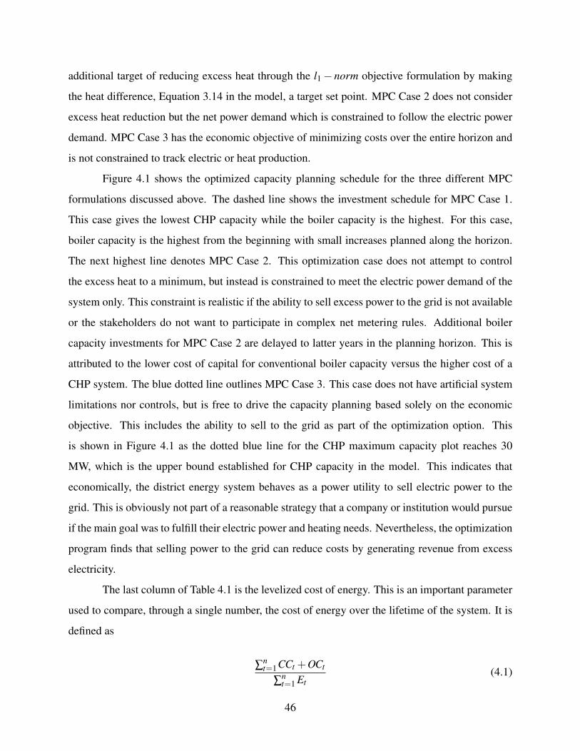
additional target of reducing excess heat through the l1− norm objective formulation by making
the heat difference, Equation 3.14 in the model, a target set point. MPC Case 2 does not consider
excess heat reduction but the net power demand which is constrained to follow the electric power
demand. MPC Case 3 has the economic objective of minimizing costs over the entire horizon and
is not constrained to track electric or heat production.
Figure 4.1 shows the optimized capacity planning schedule for the three different MPC
formulations discussed above. The dashed line shows the investment schedule for MPC Case 1.
This case gives the lowest CHP capacity while the boiler capacity is the highest. For this case,
boiler capacity is the highest from the beginning with small increases planned along the horizon.
The next highest line denotes MPC Case 2. This optimization case does not attempt to control
the excess heat to a minimum, but instead is constrained to meet the electric power demand of the
system only. This constraint is realistic if the ability to sell excess power to the grid is not available
or the stakeholders do not want to participate in complex net metering rules. Additional boiler
capacity investments for MPC Case 2 are delayed to latter years in the planning horizon. This is
attributed to the lower cost of capital for conventional boiler capacity versus the higher cost of a
CHP system. The blue dotted line outlines MPC Case 3. This case does not have artificial system
limitations nor controls, but is free to drive the capacity planning based solely on the economic
objective. This includes the ability to sell to the grid as part of the optimization option. This
is shown in Figure 4.1 as the dotted blue line for the CHP maximum capacity plot reaches 30
MW, which is the upper bound established for CHP capacity in the model. This indicates that
economically, the district energy system behaves as a power utility to sell electric power to the
grid. This is obviously not part of a reasonable strategy that a company or institution would pursue
if the main goal was to fulfill their electric power and heating needs. Nevertheless, the optimization
program finds that selling power to the grid can reduce costs by generating revenue from excess
electricity.
The last column of Table 4.1 is the levelized cost of energy. This is an important parameter
used to compare, through a single number, the cost of energy over the lifetime of the system. It is
defined as
∑nt=1CCt +OCt
∑nt=1 Et
(4.1)
46

MPC
Cas
eE
cono
mic
Obj
ectiv
eE
lect
rici
tyTa
rget
Hea
tTa
rget
Max
CH
PC
apac
ity
Max
Boi
ler
Cap
acity
Cap
ital
Cos
tO
pera
ting
Cos
t
Lev
eliz
edC
osto
fU
sabl
eE
nerg
y
13
73
9M
W70
MM
B-
TU
/hr
$14.
8MM
$290
.5M
M$2
9.90
/MW
h
23
37
13M
W20
MM
B-
TU
/hr
$16.
1MM
$230
.8M
M$2
6.20
/MW
h
33
77
30M
W5
MM
B-
TU
/hr
$32.
2MM
$323
.8M
M$3
0.10
/MW
h
Tabl
e4.
1:R
esul
tsfo
rthr
eedi
ffer
entM
PCfo
rmul
atio
nsfo
rthe
expe
cted
ener
gypr
ices
econ
omic
case
.
47

WhereCCt is the discounted capital cost at time t
OCt is the discounted operating cost at time t
Et is the usable energy generation at time t
n is the life of the systemThe sum of usable energy (Et) is the sum of both electric and usable thermal energy in
megawatt-hours, but does not account for thermal energy that is wasted through the flue gas. The
levelized cost of energy is a useful tool to evaluate which generation system option produces energy
in the most cost effective way. For the different MPC optimization cases, MPC Case 2 produces
the lowest cost in dollars per megawatt-hour of usable energy generated.
Figure 4.2 shows the effects of the MPC cases on surplus heat. It is important to note
that excess heat production from a district heating system is discarded to the atmosphere, and
electricity is exported to the grid if generation is above the system needs. Production of thermal
energy beyond the heat demand of the district energy system reduces the efficiency gains of heat
and power integration, one of the main goals of a CHP system. The l1−norm formulation of MPC
Case 1 has the lowest excess heat release because the excess heat term of the model is a variable
targeted for minimization. The control objective is effective in that it fully utilizes all available
heat in the winter season. MPC Case 2 does not reduce the excess heat generation as aggressively
as MPC Case 1, but gradually diminishes the excess heat over the 30 year horizon for both summer
and winter. MPC Case 3, as discussed earlier, has only the economic objective and thus produces
both excess electricity and likewise excess heat.
MPC formulations offer a direct way of expressing operational strategies into a capacity
planning problem and observe the effect on size and timing of capacity investment.
4.2 Utilization of Capacity
The results in the previous section reveal that although the economic objective is the main
driver for the optimization, operational objectives can be formulated into the problem. Providing
the lowest capital and operational cost also depends on how the capacity is utilized given the ad-
ditional operating objectives such as reducing excess heat production. Reducing excess heat has
a direct effect on CO2 emissions which in the long term can become an important operational ob-
48

Figu
re4.
1:C
HP
and
boile
rcap
acity
inve
stm
entp
lan
from
MPC
form
ulat
ion
base
don
thre
edi
ffer
entc
ontr
olob
ject
ives
fort
heex
pect
eden
ergy
pric
esec
onom
icca
se.
49

Figu
re4.
2:Su
rplu
she
atpr
ofile
sfo
rthe
diff
eren
tMPC
case
s.M
PCC
ase
3ha
sth
elo
wes
texc
ess
heat
forb
oth
win
tera
ndsu
mm
er.
For
win
terp
rofil
eit
goes
toze
rofo
rMPC
Cas
e3.
50

jective if carbon cutting regulations are implemented. Capacity planning has a multi-decade time
scale while operational strategy has an hourly time scale. This work merges the differences in
time scales by directly using representative diurnal load profiles for heat and electricity of winter
and summer seasons and projecting them over a 30 year horizon as illustrated earlier in Figure
3.4. The differential terms in the model directly respond to the short term dynamics for energy
generation while the differential of maximum capacity (∂mcp
∂ t) takes effect only when extra ca-
pacity is needed. The multi-scale features provide additional flexibility to the optimizer to move
manipulated variables that affect short scale economic and control objectives while simultaneously
scheduling capacity investments over the long term horizon. Figure 4.2 shows the heating profiles
for both summer and winter seasons along with the utilization of heat supply for MPC Case 1. As
mentioned earlier, MPC Case 1, has the control objective of reducing excess heat. The optimizer
achieves this by using the extra boiler capacity during the winter season to follow the heat load
with only a small fraction supplied by the heat recovery boiler. The total heat supply denoted by
the “x” marker is a perfect match with the heat demand of the winter profile. For the summer
heating profile, the heat is provided by the heat recovered from the CHP while the extra boiler
capacity set point is set at zero (boiler off) denoted by the diamond marker. The CHP system does
not follow the heat load but rather stays atop the peak demands throughout the summer horizon.
This happens because the heat generated from the turbine to meet the higher summer electric load
is enough to meet the heat demand. This strategy is found by the optimizer in order to reduce the
excess heat control variable.
In summary, the excess heat minimization objective in MPC Case 1 is achieved by changing
the capacity utilization of both winter and summer seasons. During the summer, CHP heat output
is maximized and in the winter boiler load following is recommended. This is a good strategy in
places where air quality issues are more sensitive during the winter months, and reducing excess
heat production to minimum limits is desirable to reduce combustion emissions. Traditional op-
timization and modeling approaches for capacity planning problems cannot give short-term guid-
ance on utilization of capacity because the models do not detail dynamic response of the system as
this work presents.
51

Figu
re4.
3:H
eatin
gsu
pply
profi
les
forM
PCca
se1
52

4.3 Optimization Under Different Economic Scenarios
This section contains optimization results based on different economic scenarios. The re-
sults directly reflect the effect of input economic data and not the MPC formulation. The MPC
formulation is kept constant and is based on MPC Case 2 formulation above. MPC Case 2 is
chosen because computation times are slightly lower than the other cases. As discussed in the
previous section, MPC Case 2 formulation maintains the economic objective and restricts electric
power production to meet system load. MPC Case 2 does not allow the transfer of power to the
grid.
4.3.1 Economic Scenarios Relaxed Problem Results
Optimizing capacity planning under different economic scenarios beyond the expected nat-
ural gas and electricity prices generate results that give insights on the sensitivity of the capacity
and timing of investment on energy prices. Figure 4.4 shows the CHP capacity plan for seven
different economic scenarios. The CHP capacity is lower for all cases where there is monetary
cost per short ton of CO2 emission. The higher the cost per ton, the lower the CHP capacity is
calculated to be optimal while the low economic growth case which contains the lowest energy
prices and no CO2 cost has the highest capacity. The reference case, the high economic growth,
and no greenhouse gas (GHG) concern cases converge to the same capacity. For this reason only
the plot for high economic growth case appears, the other two are hidden behind the same line.
Regardless of the economic case and magnitude of capacity, the optimizer indicates that CHP in-
vestment should be made from the beginning of the planning horizon. These results are from a
relaxed problem formulation on the CHP capacity variable (mcchp). In optimization, a relaxed
formulation means that there is no requirement for integer solution of designated variables, but
instead the entire continuous feasible space is available. Integer formulations are computationally
harder to solve, but give more realistic results. For example, turbine capacities are usually rated by
integer number (e.g. 10 MW) instead of a mixed number (e.g. 10.14 MW).
In conjunction with the CHP capacity, the boiler capacity investment schedule is give by
Figure 4.5 which shows different timings for additional boiler capacity depending on the economic
case. Additional boiler capacity is delayed for those cases that have the lowest energy prices while
53

Figure 4.4: CHP capacity schedule based on different economic cases for relaxed problem formu-lation.
those that consider CO2 emission costs request additional boiler capacity earlier in the horizon.
The optimizer finds a better objective by reducing CHP capacity and increasing investment on
the lower cost boiler capacity to fulfill the energy demands when operating costs are higher. The
reference case, high economic growth, and no GHG concern cases over lap with the same timing
and capacity plotted by the blue and cyan line in Figure 4.5.
54

Figure 4.5: Boiler capacity schedule based on different economic cases for relaxed problem for-mulation.
4.3.2 Economic Scenarios MINLP Results
Results for the mixed integer problem (MINLP) formulation are summarized in Figure 4.6
for a larger set of economic scenarios. Optimization of a wider range of economic scenarios gives
further insights about the feasibility of a CHP system. In 15 out of 20 different economic cases that
account for natural gas and electricity price fluctuations over the 30 year horizon, the optimization
results find feasible to invest in a CHP system, while only five cases suggest to make no CHP
investment and keep a boiler only system.
A histogram with the frequency of the integer solutions for CHP and boiler capacities is
given in Figure 4.7. For most of the economic scenarios, the CHP maximum capacity recommen-
dations are closely aggregated between 9 MW and 13 MW capacity, a difference of just 4 MW
in capacity. Although a 4 MW spread translates to differences in several million dollars in capital
investment, the optimization solution provides less uncertain capacity options because more infor-
mation about the system is encapsulated and solved simultaneously. It is important to mention that
for all cases where CHP capacity is cost effective, the capacity investment starts from the begin-
ning of the horizon, mirroring the relaxed problem results of Figure 4.4. Figure 4.7 also shows the
55

Figure 4.6: CHP and boiler maximum capacities by economic scenario.
frequencies of the maximum boiler capacities. Similar to the relaxed problem solution of Figure
4.5, the boiler capacity increases are distributed at different points of the horizon.
There are five cases where the optimization finds a lower objective function without CHP
investment. These results are less intuitive to understand, but underscore the benefits of large scale
dynamic optimization formulations that utilize large sets of data and solve the problem simultane-
ously for the entire horizon. The economic evaluations are performed at every step of the horizon,
thus the hidden trade offs from the economic data inputs at different time points are exploited to
find an overall lower cost objective. Discrete, steady state evaluations would never be able to com-
pare the dynamic interactions of price and demand fluctuations to differentiate the capacity size
decision over a large time horizon.
56

Figure 4.7: CHP capacity histogram (top) and boiler total capacity histogram (bottom).
57

CHAPTER 5. CONCLUSION AND FUTURE CONSIDERATIONS
This work presents a dynamic optimization framework with MPC elements for capacity
planning of an energy district system. Key conclusions from this work are summarized next.
Non-linear terms are essential to capture cost effects such as economies of scale as the op-
timizer simultaneously captures the economic and physical relationships that describe the system.
For example, although the optimal CHP capacity size varies depending on the economic scenario,
the optimizer finds that a sizable CHP capacity from the beginning of the horizon has a steeper
reduction in overall costs than a delayed CHP investment regardless of how the capacity may be
utilized.
The modeling of the district energy system along with the formulation to find the capacity
investment over a thirty year horizon is facilitated by the novel use of differential and algebraic
equations. The differential elements explicitly account for changes in capacity over time with-
out the need to explicitly discretize the model to account for time as is done in traditional linear
programming formulations. For this application, the differential terms tie together energy demand
dynamics with response time constraints, and relate the production of energy in the short time scale
to the longer term maximum capacity. This cannot be done in models that do not treat time as a
continuous, explicit variable.
This work also shows that within the dynamic optimization framework, a model predictive
control formulation of the objective function can add other control objectives beside the economic
objective. The MPC formulation inserts operational control objectives to the optimization formu-
lation to observe the effects on long term capacity planning. Different economic cases also affect
capacity and timing of the investment. This optimization framework is a tool to guide timing of
capacity investments that reflects operational strategies and multiple objectives.
For a building campus district energy system, proposing a CHP investment to meet energy
needs is a major change. From the results of this optimization study, the question of whether to
58

invest in a CHP system is answered by the optimization recommendations to make some type of
CHP investment for most economic cases from the beginning of the horizon. The other half of the
question is in regards to the size of the capacity investment. The size of the capacity investment
will depend closely on the financial incentive that the optimizer finds based on the uncertain fuel
cost and electricity price data. In contrast, without a simultaneous optimization with uncertain
parameters, CHP builders have recommend capacity options that are over fifty percent larger than
the largest optimized CHP capacity result for a system of similar size. Oversized CHP capacity
options not only increase already expensive capital expenditures, but also CHP utilization will be
more expensive because there is a greater opportunity for the gas turbine to operate at lower, less
efficient loads over the lifetime of the system.
Difficulty in solving large and highly non-linear dynamic optimization problems is some-
thing that is still problematic and subject of continuous research. This limitation is visible in this
work in using second degree polynomials instead of better fitting exponential functions for capac-
ity vs. cost relationship. The optimizer in certain cases recommends smaller increases in boiler
capacity throughout the horizon, which may be an artifact of the slightly non-linear polynomial
functions. Close to the origin, the polynomial fits are almost linear; therefore, smaller capacities
give smaller cost and potentially an artificially lower objective. Limitations also exist in this work
when formulating the problem to explicitly account for uncertainty by introducing larger amounts
of data into the problem. The optimizer handles 20,463 state variables, 18,309 total equations, and
2,872 slack variables, with over 700 degrees of freedom when considering a single economic case.
When different economic cases are simultaneously solved, the optimization solver is unable to
solve the problem. Future work should explore improving optimization solver start up procedures
as well as consideration of alternative large scale optimization solvers to diminish both the highly
non-linear and large problem limitations. Consideration of other large scale solvers will require
formulating this problem in different mathematical modeling languages like GAMS or AMPL.
To further understand and differentiate the effects of important economic parameters, fu-
ture work should explore global optimization techniques to verify global optimality from given
economic inputs. So far, this work does not include comprehensive study on the global optimality
of the solutions, but mainly focuses on a gradient based dynamic optimization strategy for energy
system capacity expansion problems.
59

This work does not attempt to show an exhaustive capacity investment schedule for a dis-
trict energy system, but rather demonstrate that a dynamic optimization framework with MPC
elements is a feasible approach to guide capacity planning of energy systems. This approach can
be expanded to larger systems such as smart grid applications where a number of interactive energy
systems with unique dynamics such as coal power plants, wind and solar renewable power sources,
energy storage, and carbon capturing systems interact to meet demands. The intrinsic dynamics,
economic, and operational targets affect capacity and timing of investments of system components.
This optimization framework brings a holistic approach to handle multiple targets and system data
within a single optimization formulation.
60
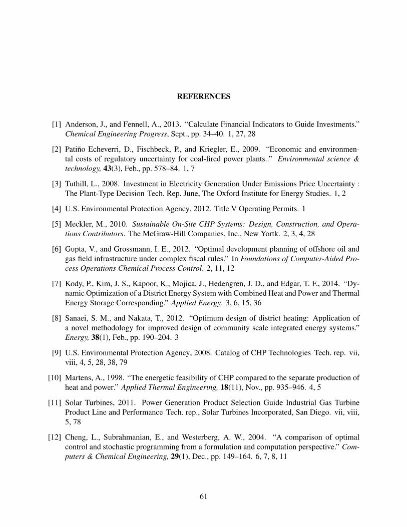
REFERENCES
[1] Anderson, J., and Fennell, A., 2013. “Calculate Financial Indicators to Guide Investments.”Chemical Engineering Progress, Sept., pp. 34–40. 1, 27, 28
[2] Patiño Echeverri, D., Fischbeck, P., and Kriegler, E., 2009. “Economic and environmen-tal costs of regulatory uncertainty for coal-fired power plants..” Environmental science &technology, 43(3), Feb., pp. 578–84. 1, 7
[3] Tuthill, L., 2008. Investment in Electricity Generation Under Emissions Price Uncertainty :The Plant-Type Decision Tech. Rep. June, The Oxford Institute for Energy Studies. 1, 2
[4] U.S. Environmental Protection Agency, 2012. Title V Operating Permits. 1
[5] Meckler, M., 2010. Sustainable On-Site CHP Systems: Design, Construction, and Opera-tions Contributors. The McGraw-Hill Companies, Inc., New Yortk. 2, 3, 4, 28
[6] Gupta, V., and Grossmann, I. E., 2012. “Optimal development planning of offshore oil andgas field infrastructure under complex fiscal rules.” In Foundations of Computer-Aided Pro-cess Operations Chemical Process Control. 2, 11, 12
[7] Kody, P., Kim, J. S., Kapoor, K., Mojica, J., Hedengren, J. D., and Edgar, T. F., 2014. “Dy-namic Optimization of a District Energy System with Combined Heat and Power and ThermalEnergy Storage Corresponding.” Applied Energy. 3, 6, 15, 36
[8] Sanaei, S. M., and Nakata, T., 2012. “Optimum design of district heating: Application ofa novel methodology for improved design of community scale integrated energy systems.”Energy, 38(1), Feb., pp. 190–204. 3
[9] U.S. Environmental Protection Agency, 2008. Catalog of CHP Technologies Tech. rep. vii,viii, 4, 5, 28, 38, 79
[10] Martens, A., 1998. “The energetic feasibility of CHP compared to the separate production ofheat and power.” Applied Thermal Engineering, 18(11), Nov., pp. 935–946. 4, 5
[11] Solar Turbines, 2011. Power Generation Product Selection Guide Industrial Gas TurbineProduct Line and Performance Tech. rep., Solar Turbines Incorporated, San Diego. vii, viii,5, 78
[12] Cheng, L., Subrahmanian, E., and Westerberg, A. W., 2004. “A comparison of optimalcontrol and stochastic programming from a formulation and computation perspective.” Com-puters & Chemical Engineering, 29(1), Dec., pp. 149–164. 6, 7, 8, 11
61

[13] Tan, L., and Chen, Y., 2009. “A general framework for solving multi-objective optimizationunder uncertainty.” 2009 IEEE 6th International Power Electronics and Motion ControlConference, 3, May, pp. 2432–2437. 6, 7
[14] Subramanyan, K., Diwekar, U. M., and Goyal, A., 2004. “Multi-objective optimization forhybrid fuel cells power system under uncertainty.” Journal of Power Sources, 132(1-2), May,pp. 99–112. 6, 10
[15] Liu, Z. F., Huang, G. H., and Li, N., 2008. “A Dynamic Optimization Approach for PowerGeneration Planning under Uncertainty.” Energy Sources, Part A: Recovery, Utilization, andEnvironmental Effects, 30(14-15), June, pp. 1413–1431. 7, 9
[16] Nagl, S., Lindenberger, D., Paper, E. W. I. W., and Economics, E., 2012. “Optimization ofpower plant investments under uncertain renewable energy development paths-A multistagestochastic programming approach.”. 7
[17] Reinelt, P. S., and Keith, D. W., 2007. “Carbon Capture Retrofits and the Cost of RegulatoryUncertainty.” Energy Journal, 28(4), pp. 101–128. 7
[18] Birge, J. R., and Louveaux, F., 1997. Introduction to Stochastic Programming. SpringerSeries in Operations Research, New York. 7, 8
[19] Fuss, S., Szolgayova, J., Obersteiner, M., and Gusti, M., 2008. “Investment under market andclimate policy uncertainty.” Applied Energy, 85(8), Aug., pp. 708–721. 8
[20] Borges, A. R., and Antunes, C. H., 2003. “A fuzzy multiple objective decision support modelfor energy-economy planning.” European Journal of Operational Research, 145, pp. 304–316. 8
[21] Tekiner, H., Coit, D. W., and Felder, F. a., 2010. “Multi-period multi-objective electricity gen-eration expansion planning problem with Monte-Carlo simulation.” Electric Power SystemsResearch, 80(12), Dec., pp. 1394–1405. 8
[22] Li, Y., Li, Y., Huang, G., and Chen, X., 2010. “Energy and environmental systems plan-ning under uncertainty-An inexact fuzzy-stochastic programming approach.” Applied Energy,87(10), Oct., pp. 3189–3211. 9, 25
[23] Qin, S., and Badgwell, T. a., 2003. “A survey of industrial model predictive control technol-ogy.” Control Engineering Practice, 11(7), July, pp. 733–764. 9
[24] Seborg, D. E., Edgar, T. F., and Mellichamp, D. A., 2004. Process Dynamics and Control.John Wiley & Sons, Hoboken. 9
[25] Flores-Tlacuahuac, A., Morales, P., and Rivera-Toledo, M., 2012. “Multiobjective Nonlin-ear Model Predictive Control of a Class of Chemical Reactors.” Industrial & EngineeringChemistry Research, 51(17), May, pp. 5891–5899. vii, 10, 12
[26] Ricardez-Sandoval, L., Budman, H., and Douglas, P., 2009. “Integration of design and controlfor chemical processes: A review of the literature and some recent results.” Annual Reviewsin Control, 33(2), Dec., pp. 158–171. 9, 10
62

[27] U.S. Department of Energy Intermountain Clean Energy Application Center, 2011. CHPProject Profiles Tech. rep. 11
[28] Gutierrez-Limon, M. A., Flores-tlacuahuac, A., and Grossmann, I., 2012. “Scheduling andcontrol using multiobjective optimization approach.” In Foundations of Computer-Aided Pro-cess Operations Chemical Process Controls. 11, 12
[29] Antunes, C., Martins, A., and Brito, I. S., 2004. “A multiple objective mixed integer linearprogramming model for power generation expansion planning.” Energy, 29(4), Mar., pp. 613–627. 11
[30] Guti, M. A., Flores-tlacuahuac, A., and Grossmann, I. E., 2012. “A Multiobjective Opti-mization Approach for the Simultaneous Single Line Scheduling and Control of CSTRs.”pp. 5881–5890. 12
[31] Parkinson, A., 2012. Optimization-Based Design. Provo. 13, 18
[32] Astrom, K. J., and Bell, R. D., 2000. “Drum-boiler dynamics.” Automatica, 36. 14
[33] Bisschop, J., 2012. AIMMS Optimization Modeling Tech. rep., Paragon Decision Technol-ogy, Bellevue. 17, 19, 21
[34] Edgar, T. F., Himmelblau, D. M., and Lasdon, L. S., 2001. Optimization of Chemical Pro-cesses., second ed. McGraw-Hill, Boston. 18, 32, 33
[35] Westner, G., and Madlener, R., 2010. Investment in New Power Generation under Uncertainty: Benefits of CHP vs Condensing Plants in a Copula-Based Analysis Tech. Rep. 12, Institutefor Future Energy Consumer Needs and Behavior, Munich. 25
[36] U.S. Energy Information Administration, 2013. Cost of Natural Gas Used in ManufacturingSector Has Fallen Tech. rep. 26
[37] U.S. Energy Information Administration, 2013. Annual Energy Outlook 2013 Tech. rep.,U.S. Energy Information Administration. vii, 26
[38] Lion Technology, 2013. Environmental Regulations Desk Reference Tech. rep., Lion Tech-nology Inc., Lafayette. 26
[39] Investopedia, 2013. Definition of Discount Rate. 27
[40] Damodaran, A., 2013. Cost of Capital by Sector Tech. rep., New York University, New York.27
[41] Trading Economics, 2013. United States Inflation Rate. 28
[42] Nagashima, M., Tsuchiya, M., and Asada, M., 2011. “Reducing the Economic Risk of LNGTank Construction under Conditions of Fluctuating Resource Prices.” Journal of Construc-tion Engineering and Management(May), pp. 382–391. 28
[43] Hedengren, J. D., 2013. APMonitor Optimization Suite. 28
63

[44] Hedengren, J. D., Shishavan, R. A., Powell, K. M., and Edgar, T. F., 2013. Nonlinear Model-ing , Estimation and Predictive Control in APMonitor. 29, 30
[45] Binder, T., Blank, L., Bock, H. G., and Bulirsch, R., 2001. “Introduction to model basedoptimization of chemical processes on moving horizons.” In Online Optimization of LargeScale Systems. pp. 295–339. 30
[46] Biegler, L. T., 2007. “An overview of simultaneous strategies for dynamic optimization.”Chemical Engineering and Processing: Process Intensification, 46(11), pp. 1043 – 1053<ce:title>Special Issue on Process Optimization and Control in Chemical Engineering andProcessing</ce:title>. 30
[47] Palm, W. J., 2010. System Dynamics., 2nd editio ed. 30
[48] Findeisen, R., Allgower, F., and Biegler, L., 2007. Assessment and future directions of non-linear model predictive control. Springer-Verlag, Berlin. 30
[49] Chittum, A., and Kaufman, N., 2011. Challenges Facing Combined Heat and Power Today:A State-by-State Assessment Tech. rep., American Council for an Energy-Efficient Economy,Washington D.C. 37
[50] Bertsekas, D. P., and Tsitsiklis, J. N., 2008. Introduction to Probability., second edi ed.Athena Scientific, Nashua. 41, 42
[51] The Mathworks, 2013. Kernel Distribution. 43
[52] Peters, M. S., Timmerhaus, K. D., and West, R. E., 2003. Plant Design and Economics forChemical Engineers., fifth ed. New York. viii, 79
64

APPENDIX A. DYNAMIC BOILER MODEL
\ b e g i n { l s t l i s t i n g } [ l a n g u a g e = ma t l a b ]
Model
P a r a m e t e r s
% b o i l e r p h y s i c a l P a r a m e t e r s
mt = 300000 % ( kg ) t o t a l m e t a l mass o f b o i l e r
C p _ b o i l e r = 0 . 4 9 % ( kJ / kg*K) h e a t c a p a c i t y o f
m e t a l
Vt = 88 %(m^3) t o t a l volume of
t h e drum , downcomer , and r i s e r s
gashhv = 3 9 . 5 % (MJ / m3) n a t u r a l gas h igh
h e a t i n g v a l u e
% steam / w a t e r p h y s i c a l P a r a m e t e r s
MW_water = 18 % M o l e c u l a r w e i gh t o f w a t e r ( kg / kmol )
t r e f f = 273 .15 % deg K,
r e f e r e n c e t e m p e r a t u r e f o r e n t h a l p h y c a l c u l a t i o n s
t c r i t = 647 .096 % ( deg K) c r i t i c a l
t e m p e r a t u r e o f w a t e r
% n e x t a r e t h e e m p i r i c a l c o n s t a n t s f o r t h e f o r m u l a s from
steam t a b l e d a t a
%t e m p s a t c o n s t a n t s
A t s a t = 6E−11
B t s a t = −2E−6
65
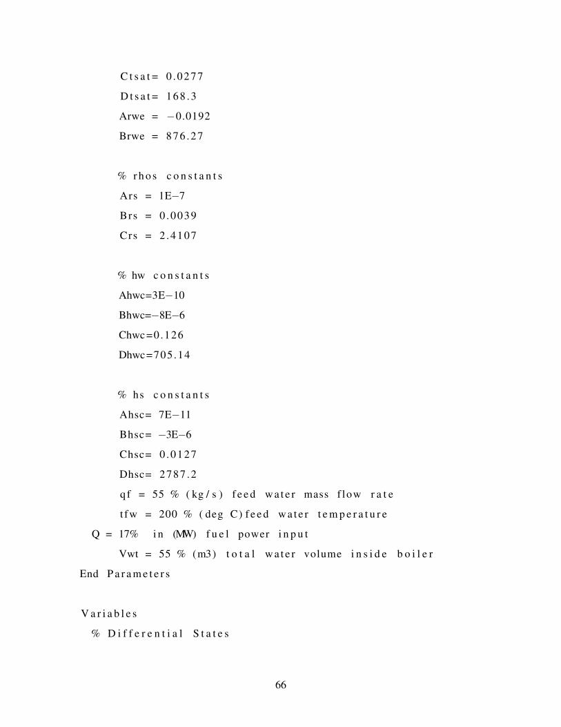
C t s a t = 0 .0277
D t s a t = 168 .3
Arwe = −0.0192
Brwe = 876 .27
% r h o s c o n s t a n t s
Ars = 1E−7
Brs = 0 .0039
Crs = 2 .4107
% hw c o n s t a n t s
Ahwc=3E−10
Bhwc=−8E−6
Chwc =0.126
Dhwc=705.14
% hs c o n s t a n t s
Ahsc= 7E−11
Bhsc= −3E−6
Chsc= 0 .0127
Dhsc= 2787 .2
q f = 55 % ( kg / s ) f e e d w a t e r mass f low r a t e
t fw = 200 % ( deg C) f e e d w a t e r t e m p e r a t u r e
Q = 17% i n (MW) f u e l power i n p u t
Vwt = 55 % (m3) t o t a l w a t e r volume i n s i d e b o i l e r
End P a r a m e t e r s
V a r i a b l e s
% D i f f e r e n t i a l S t a t e s
66

qs = 55 % ( kg / s ) s team mass f low r a t e
p = 8000 % ( kPa ) drum p r e s s u r e
t e m p _ s a t
g a s _ f l o w
V _ s t e a m _ i n s i d e
V_water
End V a r i a b l e s
I n t e r m e d i a t e s
t e m p s a t = 35 .6784* p ^ ( 0 . 2 3 5 0 )
t f = t fw +273.15 % ( deg K) f e e d w a t e r t e m p e r a t u r e
rhow = ( 3 . 3 6 5 9 E−8*p + 0 . 0 0 1 1 1 7 ) ^(−1) % i n kg /m^3
r h o s = ( 2 1 1 . 0 7 5 / p −0.00294) ^(−1) % i n kg /m^3
Vst = Vt − Vwt % t o t a l s team volume i n s i d e b o i l e r
hw = 103 .749* p ^0 .28302 % i n kJ / kg
hs = 2802 .4 − 1 .6038E−5*(p−3124.9) ^1 .73808 % i n kJ / kg
hf = ( 2 . 7 6 3 E5 *( t f − t r e f f ) −2.0901E3 *( t f ^2− t r e f f ^2 ) / 2 +
8 . 1 2 5 * ( t f ^3 − t r e f f ^3 ) / 3 −1.14116E−2*( t f ^4− t r e f f ^4 ) / 4
67

+ 9 .3701E−6*( t f ^5− t r e f f ^5 ) / 5 ) * 1 / ( MW_water *1000) % ( kJ /
kg )
% DERIVATIVE PARTS
drhow = −3.3659E−8 / (3 .3659E−8*p +0 .001117) ^2 % i n ( ( kg / m3)
/ kPa )
d r h o s = 2 1 1 . 0 7 5 / ( ( p ^2 ) * ( 2 1 1 . 0 7 5 / p − 0 . 0 0 2 9 4 ) ^2 ) %i n ( ( kg /
m3) / kPa )
dhw = 2 9 . 3 6 3 0 4 1 9 8 / p ^0.71698% i n ( kJ / kg ) / ( kPa )
dhs = −0.00002787532704*( p−3124.9) ^0 .73808 % i n ( kJ / kg ) / (
kPa )
d t s = 8 . 3 8 4 4 2 4 / p ^ 0 . 7 6 5 % ( deg C) / ( kPa )
g a s f l o w = Q/ gashhv + ( 0 . 3 / 0 . 7 ) * (Q/ gashhv ) % (m3 / s ) t o t a l
n a t u r a l gas f low r a t e ,
%assuming t h a t 70% of t h e h e a t i n g v a l u e goes t o p roduce
s team
%t h i s has t o be c a l c u l a t e d more c l o s e l y t o c a r e f u l l y
q u a n t i f y t h e gas usage , which u l t i m a t e l y i s what we
want .
e11 = rhow − r h o s
e12 = Vwt*drhow + Vst * d r h o s
e21 = rhow*hw − r h o s * hs
68

e22 = Vwt *(hw*drhow + rhow*dhw ) + Vst * ( hs * d r h o s + r h o s *
dhs ) − Vt + mt* C p _ b o i l e r * d t s
% f o r p a r a m e t e r r e p o r t i n g and compar i son t o Astrom ’ s
v a l u e s
p a r a m e t e r 1 = ( hs−hw ) * Vst * d r h o s
p a r a m e t e r 2 = r h o s * Vst * dhs
p a r a m e t e r 3 = rhow*Vwt*dhw
p a r a m e t e r 4 = mt* C p _ b o i l e r * d t s
End I n t e r m e d i a t e s
E q u a t i o n s
t e m p _ s a t = t e m p s a t
g a s _ f l o w = g a s f l o w
V _ s t e a m _ i n s i d e = Vst
V_water = Vwt
% o v e r a l l mass b a l a n c e
e11 *$Vwt+e12 *$p = qf − qs
% e ne rg y b a l a n c e
e21 *$Vwt + e22 *$p = Q*(1 E3 ) + qf * h f − qs * hs
End E q u a t i o n s
End Model
\ end { l s t l i s t i n g }
69

APPENDIX B. ENERGY SYSTEM DYNAMIC MODEL
\ b e g i n { l s t l i s t i n g } [ l a n g u a g e = ma t l a b ]
model
c o n s t a n t s
I = 1
c h p _ c a s e s = 1 % i f g r e a t e r t h a n 1 , more t h a n one economic
c a s e i s s i m u l t a n e o u s l y b e i n g s o l v e d
end c o n s t a n t s
p a r a m e t e r s
t a u 1 = . 0 0 1
t a u 2 = . 0 0 1
e l e c p r i c e [ 1 : I ] = 0 % $ /MWhr
n g p r i c e [ 1 : I ] = 0 % $ /MMBTU/ hr
demand1 = 10
demand2 = 10
h e a t 1 = 10
h e a t 2 = 10
i t i m e = 0
n a v e r a g e = 2 % t h i s i s t h e number o f y e a r s b e i n g
a v e r a g e d f o r model r e d u c t i o n ,
%i f = 1 , t h e n t h e f u l l model i s b e i n g s o l v e d
c o 2 p r i c e [ 1 : I ] = 0 %$ / m e t r i c t o n
t i m e s t e p = 0 .041667
i n f l a t i o n = 0 . 0 3
70

d i s c o u n t = 0 . 0 6
b o i l e r e f f = 0 . 8
c a p d i f f = 0 . 2
co2ng = 124 .8 %l b CO2 /MMBTU
b o i l e r _ m i n _ c a p = 5 % MMBTU/ hr
end p a r a m e t e r s
v a r i a b l e s
% f o r a l l v a r i a b l e names i n model : 1 i s f o r summer , 2 i s f o r
w i n t e r
% i f v a r i a b l e name s t a r t s w i th " i n t , " t h e n i t i s an i n t e g e r
v a r i a b l e
x_s [ 1 : I ] = 0 , >= 0 , <=30 %
x i s chp e l e c t r i c i t y p r o d u c t i o n i n MW
x_w [ 1 : I ] = 0 , >= 0 , <=30 %
x i s chp e l e c t r i c i t y p r o d u c t i o n i n MW
y_s [ 1 : I ] = 20 , >=0 % y i s
t h e chp h e a t o u t p u t a s s team or h o t w a t e r
y_w [ 1 : I ] = 20 , >=0 % y i s
t h e chp h e a t o u t p u t a s s team or h o t w a t e r
b_s [ 1 : I ] = 1 , >=0 , <=100
b_w [ 1 : I ] = 1 , >=0 , <=100
u_s [ 1 : I ] = 1 , >=0 , <=100
% u i s t h e s e t p o i n t f o r t u r b i n e
u_w [ 1 : I ] = 1 , >=0 , <=100
% u i s t h e s e t p o i n t f o r t u r b i n e
v_s [ 1 : I ] = 1 , >=0 , <=100
% v i s t h e s e t p o i n t f o r b o i l e r
71
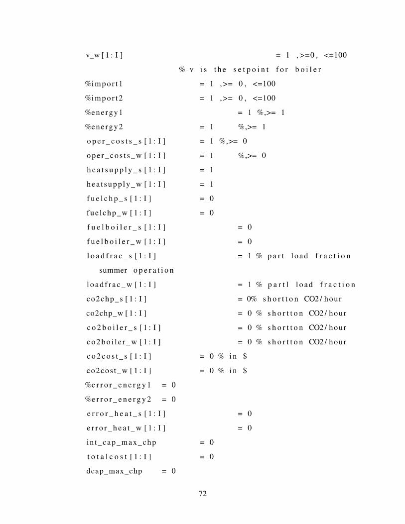
v_w [ 1 : I ] = 1 , >=0 , <=100
% v i s t h e s e t p o i n t f o r b o i l e r
%i m p o r t 1 = 1 , >= 0 , <=100
%i m p o r t 2 = 1 , >= 0 , <=100
%energy1 = 1 %,>= 1
%energy2 = 1 %,>= 1
o p e r _ c o s t s _ s [ 1 : I ] = 1 %,>= 0
o p e r _ c o s t s _ w [ 1 : I ] = 1 %,>= 0
h e a t s u p p l y _ s [ 1 : I ] = 1
h e a t s u p p l y _ w [ 1 : I ] = 1
f u e l c h p _ s [ 1 : I ] = 0
fue lchp_w [ 1 : I ] = 0
f u e l b o i l e r _ s [ 1 : I ] = 0
f u e l b o i l e r _ w [ 1 : I ] = 0
l o a d f r a c _ s [ 1 : I ] = 1 % p a r t l o a d f r a c t i o n
summer o p e r a t i o n
l o a d f r a c _ w [ 1 : I ] = 1 % p a r t l l o a d f r a c t i o n
co2chp_s [ 1 : I ] = 0% s h o r t t o n CO2 / hour
co2chp_w [ 1 : I ] = 0 % s h o r t t o n CO2 / hour
c o 2 b o i l e r _ s [ 1 : I ] = 0 % s h o r t t o n CO2 / hour
c o 2 b o i l e r _ w [ 1 : I ] = 0 % s h o r t t o n CO2 / hour
c o 2 c o s t _ s [ 1 : I ] = 0 % i n $
co2cos t_w [ 1 : I ] = 0 % i n $
%e r r o r _ e n e r g y 1 = 0
%e r r o r _ e n e r g y 2 = 0
e r r o r _ h e a t _ s [ 1 : I ] = 0
e r r o r _ h e a t _ w [ 1 : I ] = 0
in t_cap_max_chp = 0
t o t a l c o s t [ 1 : I ] = 0
dcap_max_chp = 0
72

i c o s t s _ c a p _ c h p = 0
cap_npv = 0
c a p i t a l _ c o s t s = 0
%excess_power1 = 0
%excess_power2 = 0
n e t p o w e r _ s [ 1 : I ] = 0 , <= 0 % add t h e <= 0
c o n s t r a i n t i f you want t o remove a b i l i t y
%t o s e l l e l e c t r i c i t y t o g r i d ( No n e t p o s i t i v e
power p r o d u c t i o n )
netpower_w [ 1 : I ] = 0 , <= 0 % add t h e <= 0
c o n s t r a i n t i f you want t o remove a b i l i t y
%t o s e l l e l e c t r i c i t y t o g r i d ( No n e t p o s i t i v e
power p r o d u c t i o n )
f u e l e f f _ s [ 1 : I ] = 1
f u e l e f f _ w [ 1 : I ] = 1
i n t _ b o i l e r _ s t e p = 0
cap_max_b = 0
dcap_max_b = 0
i c o s t s _ c a p _ b = 0
ne tpower_co2 = 0
end v a r i a b l e s
e q u a t i o n s
%**************** DEMAND PROFILES ************
%e r r o r _ e n e r g y 1 = ene rgy1 − demand1
%e r r o r _ e n e r g y 2 = ene rgy2 − demand2
e r r o r _ h e a t _ s [ 1 : I ] = h e a t s u p p l y _ s [ 1 : I ] −
h e a t 1
e r r o r _ h e a t _ w [ 1 : I ] = h e a t s u p p l y _ w [ 1 : I ] −
h e a t 2
73

%e r r o r _ e n e r g y 1 >= 0
%e r r o r _ e n e r g y 2 >= 0
e r r o r _ h e a t _ s [ 1 : I ] >= 0
e r r o r _ h e a t _ w [ 1 : I ] >= 0
%**************** DYNAMIC SYSTEM ************
t a u 1 * $x_s [ 1 : I ] + x_s [ 1 : I ] = u_s [ 1 : I ] % dynamic e q u a t i o n
f o r chp summer
t a u 2 *$x_w [ 1 : I ] + x_w [ 1 : I ] = u_w [ 1 : I ] % dynamic e q u a t i o n
f o r chp w i n t e r
t a u 1 * $b_s [ 1 : I ] + b_s [ 1 : I ] = v_s [ 1 : I ] % dynamic e q u a t i o n
f o r b o i l e r summer
t a u 2 *$b_w [ 1 : I ] + b_w [ 1 : I ] = v_w [ 1 : I ] % dynamic e q u a t i o n
f o r b o i l e r w i n t e r
y_s [ 1 : I ] = −0.0817* x_s [ 1 : I ] ^2+5 .6547* x_s [ 1 : I ] % h e a t
o u t p u t i n MMBTU/ hr a s s team or h o t w a t e r from HRSG
y_w [ 1 : I ] = −0.0817*x_w [ 1 : I ] ^2+5 .6547* x_w [ 1 : I ] % h e a t
o u t p u t i n MMBTU/ hr a s s team or h o t w a t e r from HRSG
h e a t s u p p l y _ s [ 1 : I ] = y_s [ 1 : I ] + b_s [ 1 : I ] %t o t a l h e a t
s u p p l y i n MMBTU/ hr summer
h e a t s u p p l y _ w [ 1 : I ] = y_w [ 1 : I ] + b_w [ 1 : I ] %t o t a l h e a t
s u p p l y i n MMBTU/ hr w i n t e r
n e t p o w e r _ s [ 1 : I ] = x_s [ 1 : I ] − demand1 % i f p o s i t i v e , t h e n
e x p o r t i n g power , n e g a t i v e i s i m p o r t i n g power
netpower_w [ 1 : I ] = x_w [ 1 : I ] − demand2
in t_cap_max_chp >= x_s [ 1 : I ]
in t_cap_max_chp >= x_w [ 1 : I ]
$ in t_cap_max_chp >= 0
dcap_max_chp = $in t_cap_max_chp
74

cap_max_b = b o i l e r _ m i n _ c a p * i n t _ b o i l e r _ s t e p
cap_max_b >= b_s [ 1 : I ]
cap_max_b >= b_w [ 1 : I ]
$cap_max_b >= 0
dcap_max_b = $cap_max_b
%**************** FUEL CONSUMPTIONS EVALUATIONS ************
l o a d f r a c _ s [ 1 : I ] = x_s [ 1 : I ] / ( in t_cap_max_chp + 10^(−6) ) %
p a r t l o a d f r a c t i o n summer o p e r a t i o n
l o a d f r a c _ w [ 1 : I ] = x_w [ 1 : I ] / ( in t_cap_max_chp + 10^(−6) ) %
p a r t l o a d f r a c t i o n w i n t e r o p e r a t i o n
f u e l e f f _ s [ 1 : I ] = 0 .9044* l o a d f r a c _ s [ 1 : I ] +
0 .0956 % s i m p l i f i e d e q u a t i o n
f u e l e f f _ w [ 1 : I ] = 0 .9044* l o a d f r a c _ w [ 1 : I ] +
0 .0956
f u e l c h p _ s [ 1 : I ] = (−0.1361* x_s [ 1 : I ] ^2 + 13 .347*
x_s [ 1 : I ] ) / f u e l e f f _ s [ 1 : I ] % summer f u e l c o n s u m p t i o n s o f
gas t u r b i n e i n MMBTU/ hr
fue lchp_w [ 1 : I ] = (−0.1361*x_w [ 1 : I ] ^2 + 13 .347*
x_w [ 1 : I ] ) / f u e l e f f _ w [ 1 : I ] % w i n t e r f u e l c o n s u m p t i o n s o f
gas t u r b i n e i n MMBTU/ hr
f u e l b o i l e r _ s [ 1 : I ] = b_s [ 1 : I ] / b o i l e r e f f % f u e l
c o n s u m p t i o n s o f b o i l e r i n MMBTU/ hr
f u e l b o i l e r _ w [ 1 : I ] = b_w [ 1 : I ] / b o i l e r e f f % f u e l
c o n s u m p t i o n s o f b o i l e r i n MMBTU/ hr
%**************** CO2 EVALUATIONS ***********************
co2chp_s [ 1 : I ] = ( ( f u e l c h p _ s [ 1 : I ]* co2ng )
/ 2 0 0 0 ) % s h o r t t o n CO2 / hour
co2chp_w [ 1 : I ] = ( ( fue lchp_w [ 1 : I ]* co2ng )
/ 2 0 0 0 ) % s h o r t t o n CO2 / hour
75

c o 2 b o i l e r _ s [ 1 : I ] = ( ( f u e l b o i l e r _ s [ 1 : I ]*
co2ng ) / 2 0 0 0 ) % s h o r t t o n CO2 / hour
c o 2 b o i l e r _ w [ 1 : I ] = ( ( f u e l b o i l e r _ w [ 1 : I ]*
co2ng ) / 2 0 0 0 ) % s h o r t t o n CO2 / hour
ne tpower_co2 = ( co2chp_s [ 1 : I ] +
co2chp_w [ 1 : I ] + c o 2 b o i l e r _ s [ 1 : I ] + c o 2 b o i l e r _ s [ 1 : I ] +
c o 2 b o i l e r _ w [ 1 : I ] ) * ( 0 . 5 * 3 6 5 * n a v e r a g e )
%**************** COST EVALUATIONS **********************
i c o s t s _ c a p _ c h p = (−0.0069*( t i m e s t e p * dcap_max_chp ) ^2 +
1 . 3 3 5 1 * ( t i m e s t e p * dcap_max_chp ) ) * ( 1 0 ^ 6 ) *(1 + i n f l a t i o n )
^ i t i m e % f u n c t i o n t o c a l c u l a t e i n v e s t m e n t c o s t i n $
i c o s t s _ c a p _ b = 2*(−39.504*( t i m e s t e p * dcap_max_b ) ^2 +
29900*( t i m e s t e p * dcap_max_b ) ) * (1 + i n f l a t i o n ) ^ i t i m e %%
f u n c t i o n t o c a l c u l a t e i n v e s t m e n t c o s t i n $
cap_npv = i c o s t s _ c a p _ c h p / ( ( 1 + d i s c o u n t ) ^
i t i m e ) + i c o s t s _ c a p _ b / ( ( 1 + d i s c o u n t ) ^ i t i m e ) % NPV of
c a p i t a l i n v e s t m e n t i n $
c o 2 c o s t _ s [ 1 : I ] = ( co2chp_s [ 1 : I ] + c o 2 b o i l e r _ s [ 1 :
I ] ) * c o 2 p r i c e [ 1 : I ] * ( 9 0 7 . 1 8 5 / 1 0 0 0 ) % i n $ ,
( 9 0 7 . 1 8 5 / 1 0 0 0 ) i s t h e c o n v e r s i o n f a c t o r from s h o r t t o n
t o m e t r i c t o n
co2cos t_w [ 1 : I ] = ( co2chp_w [ 1 : I ] + c o 2 b o i l e r _ w [ 1 :
I ] ) * c o 2 p r i c e [ 1 : I ] * ( 9 0 7 . 1 8 5 / 1 0 0 0 ) % i n $ ,
( 9 0 7 . 1 8 5 / 1 0 0 0 ) i s t h e c o n v e r s i o n f a c t o r from s h o r t t o n
t o m e t r i c t o n
o p e r _ c o s t s _ s [ 1 : I ] = ( ( n g p r i c e [ 1 : I ]* f u e l c h p _ s [ 1 : I ] +
n g p r i c e [ 1 : I ]* f u e l b o i l e r _ s [ 1 : I ] − ( 1 ) * e l e c p r i c e [ 1 : I ]*
n e t p o w e r _ s [ 1 : I ] + c o 2 c o s t _ s [ 1 : I ] ) * 0 . 5 * 3 6 5 ) / ( ( 1 +
d i s c o u n t ) ^ i t i m e ) * n a v e r a g e % i n $ ( summer )
76

o p e r _ c o s t s _ w [ 1 : I ] = ( ( n g p r i c e [ 1 : I ]* fue lchp_w [ 1 : I ] +
n g p r i c e [ 1 : I ]* f u e l b o i l e r _ w [ 1 : I ] − ( 1 ) * e l e c p r i c e [ 1 : I ]*
netpower_w [ 1 : I ] + co2cos t_w [ 1 : I ] ) * 0 . 5 * 3 6 5 ) / ( ( 1 +
d i s c o u n t ) ^ i t i m e ) * n a v e r a g e % i n $ ( w i n t e r )
c a p i t a l _ c o s t s = cap_npv % i n $
t o t a l c o s t [ 1 : I ] = o p e r _ c o s t s _ s [ 1 : I ] + o p e r _ c o s t s _ w [ 1 : I ]
% i n $
%**************** o b j e c t i v e F u n c t i o n
**********************
min imize t o t a l c o s t [ 1 : I ]
min imize c a p i t a l _ c o s t s * c h p _ c a s e s
end e q u a t i o n s
end model
\ end { l s t l i s t i n g }
77

APPENDIX C. CHP CORRELATIONS
Figure C.1: Data and polynomial from [11] for CHP heat supply Equation 3.13.
Figure C.2: Data and polynomial from [11] for CHP natural gas consumption Equation 3.19.
78

Figure C.3: Data and polynomial from [9] for CHP capital cost Equation 3.24
Figure C.4: Data and polynomial from [52] for boiler capital cost Equation 3.25.
79