A dynamic model using monitoring data and watershed characteristics to project fish tissue mercury...

A Dynamic Model Using Monitoring Data and WatershedCharacteristics to Project Fish Tissue Mercury Concentrationsin Stream SystemsCaroline Chan,*y John F Heinbokel,z John A Myers,§ and Robert R JacobsyyEnvironmental and Occupational Health Sciences, School of Public Health and Information Sciences, University of Louisville,485 E. Gray Street, Louisville, Kentucky 40202, USAzHealth Management and System Sciences, School of Public Health and Information Sciences, University of Louisville and Center forInterdisciplinary Excellence in System Dynamics, Barboursville, Virginia, USA§Bioinformatics and Biostatistics, School of Public Health and Information Sciences, University of Louisville, Louisville, Kentucky, USA

(Submitted 2 November 2011; Returned for Revision 9 December 2011; Accepted 14 February 2012)

ABSTRACTA complex interplay of factors determines the degree of bioaccumulation of Hg in fish in any particular basin. Although

certain watershed characteristics have been associated with higher or lower bioaccumulation rates, the relationships between

these characteristics are poorly understood. To add to this understanding, a dynamic model was built to examine these

relationships in stream systems. The model follows Hg from the water column, through microbial conversion and subsequent

concentration, through the foodweb topiscivorous fish. Themodelwas calibrated to7basins in Kentucky and further evaluated

by comparing output to 7 sites in, or proximal to, the Ohio River Valley, an underrepresented region in the bioaccumulation

literature.Water quality andbasin characteristicswere inputs into themodel,with tissue concentrations ofHgofgeneric trophic

level 3, 3.5, and4fish theoutput. Regulatory andmonitoringdatawereused to calibrate andevaluate themodel.Mean average

prediction error for Kentucky siteswas 26%,whereasmean error for evaluation siteswas 51%. Variabilitywithin natural systems

can be substantial andwas quantified for fish tissue by analysis of theUSGeological Survey National FishDatabase. This analysis

pointed to theneed formore systematic samplingoffish tissue.Analysis ofmodel output indicated thatparameters that had the

greatest impact on bioaccumulation influenced the system at several points. These parameters included forested andwetlands

coverageandnutrient levels. Factors thatwere less sensitivemodified the systematonly1point and included theunfiltered total

Hg input and the portion of the basin that is developed. Integr Environ Assess Manag � 2012 SETAC

Keywords: Fish tissue Hg Bioaccumulation Stream systems Dynamic modeling Watershed characteristics

INTRODUCTIONMercury (Hg) is a potent neurotoxin with the developing

fetus at greatest risk for adverse outcomes. In the 1999–2002National Health and Nutrition Examination Study, 6% ofwomen of childbearing age were found to have blood Hglevels at or above the US Environmental Protection Agency(USEPA) level of safety (CDC 2004). The largest source ofexposure to Hg is from fish consumption (USEPA 2009). Asof 2010, Hg contamination is responsible for fish consump-tion advisories on over 1.2 million miles (1.9 million km) ofthe nation’s rivers (USEPA 2011). The problem is bothnational and global in perspective and without a clearunderstanding of the relationship between the environmentaland physiological disposition of Hg, effective strategies toreduce contamination have not been forthcoming.

The source of Hg contamination in most stream systems isfrom atmospheric deposition, both from global and morelocal or regional sources. Atmospheric Hg makes its way intoaquatic systems through wet and dry deposition eitherdirectly to the waterway or through terrestrial compartments.Organic matter in soil often sequesters Hg, releasing it slowlyover time. A whole ecosystem study of changes in loading of

Hg to a lake system found an initial rapid response. However,the rapid change came from the Hg that was depositeddirectly to the lake surface and a much slower response wasnoted in the loading of Hg from the watershed (Harris et al.2007). For stream systems, which receive almost all Hgloading from the watershed, reductions in local and regionalemissions of Hg may not result in substantial reductions infish tissue levels for some time. Fish tissue Hg levels can varywidely between basins, and understanding the differentcharacteristics of these basins may help regulators determinewhich stream systems are most likely to have elevated Hglevels and also envisage the impact proposed changes in awatershed will have on fish tissue levels.

The dynamics of Hg transport and transformation in streamsystems have received increased research attention but arestill not well understood. The degree of bioaccumulation in asystem is dependent on the interaction of multiple variables,and such complex systems often react to changes inunexpected ways. Although the dynamics are complex,several factors have been found to be associated with higherfish tissue Hg concentrations in stream systems. Ward,Nislow, and Folt (2010b) have designated this collectionof watershed characteristics ‘‘bioaccumulation syndrome.’’Characteristics associated with increased bioaccumulation ofmethylmercury (MeHg) include connectivity to wetlands,low pH, and factors that contribute to lower levels ofproductivity such as low nutrient levels and light limitation.Every stream system has a unique set of characteristics thatinteract to either increase or decrease bioaccumulation.

Integrated Environmental Assessment and Management� 2012 SETAC 1

All Supplemental Data may be found in the online version of this article.

* To whom correspondence may be addressed: [email protected]

Published online 21 February 2012 in Wiley Online Library

(wileyonlinelibrary.com).

DOI: 10.1002/ieam.1302

Enviro

nmenta

lManagement

Amass balance, mechanistic model was built that examinesthe movement of Hg in stream systems from water column tofish tissue. The model is controlled by a series of simulatedmechanisms or processes that control the movement of Hgthrough the system. The model is dynamic in the sense that,even at steady state, the dynamics of Hg can be quantified as itmoves through the various stock and flow components. Themodel was also constructed to be dynamic in the sense ofbeing responsive to changes in Hg loading as a result ofpotential policy scenarios. If the relevant components andrelationships of the system are properly accounted for, themodel can be used to credibly project outcomes of ‘‘what if?’’scenarios.

Basins used to calibrate and evaluate the model wereprimarily from the Ohio River Valley, a region that has notbeen well represented in the literature examining Hgbioaccumulation. These sites exhibit considerable variationin land use and land cover and span several physiographicregions, from mountainous, heavily forested basins in theAppalachian Highlands to basins in the Interior Plains that arehighly cultivated. Although increased bioaccumulation hasbeen associated with wetlands coverage and has been a focusof research (Scudder et al. 2009; Warner et al. 2005),wetlands coverage is minimal in the Ohio River Valley(Emery and Spaeth 2011; White et al. 2005). This regionoffers the unique opportunity to examine the relationshipsbetween other drivers of Hg bioaccumulation.

The purpose of this project was to create a tool to assistregulatory decision makers in the process of determiningwhere and how resources can be used to protect populationsfrom adverse Hg exposures. Because the intended users areregulators, existing data from readily available regulatorysources were used as inputs. The objective was to gain insightinto how the unique characteristics of basins in this regioninteract to impact the bioaccumulation process. This insightcan then be used to determine which basins are likely to haveelevated fish tissue levels or shed light on the impact ofproposed changes in land cover or other watershed character-istics, or the responsiveness of a basin to reductions in Hgloading.

This study describes the second step in the development ofan overall model that will simulate Hg movement fromatmospheric sources to biomarkers of exposure of susceptiblehuman populations. The scope of this bioaccumulation modelis to predict fish tissue Hg levels in generic trophic level (TL)3, 3.5, and 4 fish given watershed characteristics and watercolumn Hg levels. The model focuses on the processing of Hgin the water column and its movement through the food web.The modeled fish tissue Hg concentration will be used as aninput into the model developed previously to projectbiomarkers of exposure for specified populations, describedin Chan et al. (2011). This article describes the development,calibration and evaluation, strengths, and limitations of thebioaccumulation model and discusses the interactions of thefactors that impact bioaccumulation in the modeled basins.

MODEL DEVELOPMENTLand cover and water chemistry data were inputs into the

model and were assumed to be at steady state. Fish tissueMeHg was the output. Model output was compared to actualfish tissue data to determine model accuracy.

The model was built with STELLA, version 9.0.3 (iseesystems, Lebanon, NH), a dynamic modeling program that

uses stocks and flows to simulate the storage and movementor changes of the components in a system. The system beingmodeled is a stream, and the variable that moves or changesin that system is Hg. The basic structure of the model isdescribed below and shown in Figure 1. A more detailedrepresentation of the model and documentation of allmodel equations are given in Supplemental Data (availableonline).

Basic structure

Hg enters the system through the flow ‘‘IHg Inflow.’’Inorganic mercury (IHg) moves into the INORGANIC Hg INWATER stock. From this stock, the Hg can move out of thesystem by flowing downstream or be deposited throughsedimentation to the streambed, represented by the IHg INSTREAMBED stock. This stock also represents any IHg thatmay be moved to the floodplain or retained by woody debrisor held within the system by any other means. Basins withextensive wetlands have been associated with high MeHgconcentrations. However, the location of microbial conver-sion of IHg to MeHg is less certain for basins with little or nowetlands. The literature suggests that this conversion occursin the biofilm associated with algal communities (Bell and

Figure 1. The STELLA model showing the transformation and movement of

Hg from water column through bioaccumulation in fish.

2 Integr Environ Assess Manag xxx, 2012—C Chan et al.

Scudder 2007; Desrosiers et al. 2006; Tsui et al. 2009, 2010).Because of this association, the model depicts the movementof the IHg in the streambed, after microbial conversion toMeHg, as moving directly into the TROPHIC LVL 1 stock.The TROPHIC LVL 1 stock represents the MeHg containedwithin the periphyton as defined in the broad sense asincluding the community of algae, bacteria, fungi, andexudates. The MeHg can follow 1 of 3 pathways out of theTROPHIC LVL 1 stock. It can diffuse into the water columnand be lost downstream; it can be contained within thedeclining periphyton and subsequently enter the detritalpathway, or it can be consumed by TL2 organisms. Livingorganisms with their associated MeHg are assumed to remainwithin the stream system. Loss of Hg to the system is throughmovement to detritus and then loss downstream.

The bioaccumulation process is represented by movementof MeHg from 1 TL to the next, with a ‘‘Death’’ flowremoving a portion of the MeHg at each TL. All MeHg inTL4 eventually moves into the ‘‘Death’’ flow for that level.The ‘‘Death’’ flows move MeHg to the MeHg IN DETRITUSstock. From there, the MeHg can exit the system by being lostdownstream or be recycled into the bioaccumulation processby consumption from TL2 organisms.

The bioaccumulation of MeHg through the food web isrepresented by a series of stocks labeled as TLs. The mass ofMeHg needed in each is calculated by determining thebiomass of each TL and determining the concentration ofMeHg based on the previous TL. The determination of thebiomass of TL1 is discussed below. The concentration ofMeHg in each TL is then a function of the mass of MeHg inthat TL and the corresponding biomass.

To determine the mass of MeHg that flows to subsequentTLs, trophic transfer factors (TTFs) are used. The TTF is theratio of MeHg concentrations of TLn to TLn�1. A suggestedmean value from several studies is given in the Mercury StudyReport to Congress Volume III, Appendix D (USEPA 1997).For a given amount of MeHg, the eutrophic system, with alarger crop of algae, will distribute the MeHg through a largernumber of algal cells resulting in a dilution effect at the baseof the food web (Chen and Folt 2005). This effect, calledbloom dilution, affects all subsequent levels of the food chain.In addition, the algae in high-nutrient systems produce morebiomass per unit ingested by consumers than in nutrient-poorsystems, an effect called somatic growth dilution (Karimiet al. 2007). Bloom dilution and somatic growth dilution maylead to eutrophic systems having lower trophic transferfactors than oligotrophic systems (Karimi et al. 2007;Pickhardt et al. 2002). These effects were combined in afunction called ‘‘bloom growth dilution’’ and used to adjustthe TTFs. The output of the graphical function is dependenton the mean productivity index, described below. Theadjusted TTF is used to determine a target MeHg concen-tration and the corresponding mass of MeHg needed toachieve that concentration. The mass already resident in thestock is then subtracted from the amount needed to achievethe ideal concentration and that mass of MeHg is moved tothe next TL.

The death flows for each TL move MeHg into the MeHgIN DETRITUS stock. For primary producers, the death flowis controlled by the seasonal pattern of periphyton loss, withhighest loss in fall. When moving to subsequent TLs, lifespantends to increase. For TL2, the assumption is made thatorganisms live for 1 year. The flow is controlled by removing

1/12 of the mass each month. For TL3, the mortality rate forbluegill, 0.56/year, was used to determine loss of MeHgthrough death. TL4 used the mean mortality rate forpredatory fish found in Kentucky, 0.36/year (Froese andPauly 2011).

MeHg IN DETRITUS represents the MeHg found innonliving organic matter in the system. Some of this matter islost downstream based on retention whereas the remainder istaken up by detritivores, accounted for in TL2 for this model.

Subroutines

Model subroutines simulate the interaction of factors thatimpact the basic structure of the model at key points.Subroutines are shown in Figure 2.

Inorganic mercury input. The Hg Input sector determines theamount of Hg that enters the system. For stream systems withatmospheric deposition and low wetlands coverage, theportion of total mercury (THg) that is organic is typicallyless than 6% (Krabbenhoft et al. 1999). Because the amountof MeHg is minimal, the assumption is made that 100% ofunfiltered THg input is inorganic. The mass of unfiltered THginput is calculated by multiplying the mean monthlyunfiltered THg concentration by the mean monthly flow.Particulate-bound Hg is not available for conversion to MeHg,and, in the short term, is not available for bioaccumulation.Brigham et al. (2009) studied 8 streams representing a diverserange of land cover and climate characteristics. Althoughindividual samples varied more widely, the median dissolvedHg for the 7 of 8 sites was in the neighborhood of 1 ng/L orless. The exception, with a median of 4.92 ng/L, was a riverwith an exceptionally large fraction of its basin with wetlandscoverage. Balogh et al. (1997) found that the concentration ofdissolved Hg remained relatively constant whereas unfilteredTHg varied widely in association with suspended solids. In thestudy by Balogh et al. (1997), the range of dissolved Hg was0.2–0.7 ng/L. Several additional sites on the upper MississippiRiver showed little variation and had a maximum ofapproximately 1 ng/L. Additional studies found ranges ofdissolved IHg that were as high as 2–3 ng/L (Balogh et al.2008; Dittman et al. 2009; Shanley et al. 2008; Tsui andFinlay 2011). These higher values were associated with higherconcentrations of dissolved organic carbon (DOC), a relation-ship well established in the literature (Brigham et al. 2009).Dissolved organic carbon data were not available for theKentucky sites.

In this model, only the dissolved Hg enters the modeledstream system, and the particulate-bound Hg is ignored. Themodel reflects the stable dissolved IHg concentration by usingthe minimum function in STELLA. This function returns theminimum of either the mean THg concentration or 1 ng/L asthe Hg input into the model. Because a lower pH andconnectivity to wetlands are associated with an increasedavailability of IHg for methylation, adjustments are made tothe minimum value for wetlands coverage and pH. Anincreasing portion of the unfiltered THg is designated asdissolved as wetlands coverage increases and the pH becomesmore acidic.

Retention. IHg input into the model is determined by themeasured mean concentration and monthly discharge, whichis the assumed throughput of water in the system for the

Dynamic Model of Fish Tissue Hg in Streams— Integr Environ Assess Manag xxx, 2012 3

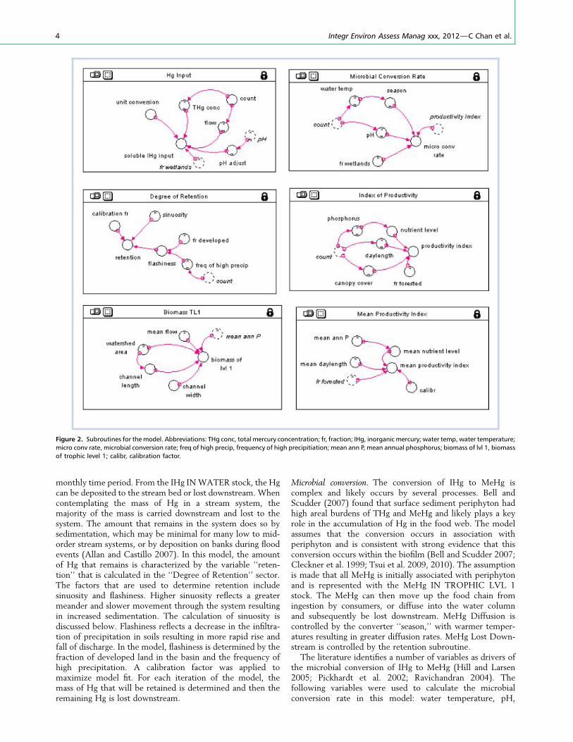
monthly time period. From the IHg INWATER stock, the Hgcan be deposited to the stream bed or lost downstream. Whencontemplating the mass of Hg in a stream system, themajority of the mass is carried downstream and lost to thesystem. The amount that remains in the system does so bysedimentation, which may be minimal for many low to mid-order stream systems, or by deposition on banks during floodevents (Allan and Castillo 2007). In this model, the amountof Hg that remains is characterized by the variable ‘‘reten-tion’’ that is calculated in the ‘‘Degree of Retention’’ sector.The factors that are used to determine retention includesinuosity and flashiness. Higher sinuosity reflects a greatermeander and slower movement through the system resultingin increased sedimentation. The calculation of sinuosity isdiscussed below. Flashiness reflects a decrease in the infiltra-tion of precipitation in soils resulting in more rapid rise andfall of discharge. In the model, flashiness is determined by thefraction of developed land in the basin and the frequency ofhigh precipitation. A calibration factor was applied tomaximize model fit. For each iteration of the model, themass of Hg that will be retained is determined and then theremaining Hg is lost downstream.

Microbial conversion. The conversion of IHg to MeHg iscomplex and likely occurs by several processes. Bell andScudder (2007) found that surface sediment periphyton hadhigh areal burdens of THg and MeHg and likely plays a keyrole in the accumulation of Hg in the food web. The modelassumes that the conversion occurs in association withperiphyton and is consistent with strong evidence that thisconversion occurs within the biofilm (Bell and Scudder 2007;Cleckner et al. 1999; Tsui et al. 2009, 2010). The assumptionis made that all MeHg is initially associated with periphytonand is represented with the MeHg IN TROPHIC LVL 1stock. The MeHg can then move up the food chain fromingestion by consumers, or diffuse into the water columnand subsequently be lost downstream. MeHg Diffusion iscontrolled by the converter ‘‘season,’’ with warmer temper-atures resulting in greater diffusion rates. MeHg Lost Down-stream is controlled by the retention subroutine.

The literature identifies a number of variables as drivers ofthe microbial conversion of IHg to MeHg (Hill and Larsen2005; Pickhardt et al. 2002; Ravichandran 2004). Thefollowing variables were used to calculate the microbialconversion rate in this model: water temperature, pH,

Figure 2. Subroutines for themodel. Abbreviations: THg conc, total mercury concentration; fr, fraction; IHg, inorganic mercury; water temp, water temperature;

micro conv rate, microbial conversion rate; freq of high precip, frequency of high precipitiation; mean ann P, mean annual phosphorus; biomass of lvl 1, biomass

of trophic level 1; calibr, calibration factor.


fraction wetlands, fraction forested, productivity index, andday length. Determination of this rate occurs in the ‘‘Micro-bial Conversion Rate’’ sector. Each of these variables wasscaled to a 0–1 range and then weighted so that the fullweights of the variables added to 1. This value is thenmultiplied by 0.36, the range of microbial conversion ratesfound in Warner et al. (2005) giving an estimate of themicrobial conversion rate found in stream systems. The meanmonthly water temperature is converted to a graphicalfunction called ‘‘season’’ that reflects the increase in primaryproducer growth during warmer weather.

Productivity index. An index is produced for the effect ofproductivity on the microbial conversion rate. Periphytonmats are thought to contribute to increased methylation rates.As mats grow and become denser, small anoxic microzoneswithin the mat may develop. The large surface area within themat favors microbial growth. The bacterial community, alongwith the oxic and anoxic borders, promotes conversion of IHgto MeHg (Mauro et al. 2002; Tsui et al. 2010; Ward et al.2010b). This effect is accounted for in the ‘‘Index ofProductivity’’ sector. Phosphorus was assumed to be thelimiting nutrient for all sites and was used as a surrogate forpotential productivity. In stream systems, light often limitsproductivity. Light limitation was introduced to the index ofproductivity by including the fraction forested, canopy cover,and monthly length of daylight hours. ‘‘Canopy cover’’ is agraphical function that relates the effects of season to thefraction of the watershed that is forested. Stream productivityis often greatest in forested basins before spring leaf out. Thegraphical function limits the effect of shading to months withcanopy coverage.

Biomass TL1. Although the biomass of primary producersvaries greatly with the seasons, this pattern diminishes forsubsequent TLs. The biomass of TL1 is used to estimate thebiomass of all subsequent TLs. To minimize this seasonalpattern in higher TLs, the mean annual biomass of TL1 isestimated in the ‘‘Biomass TL1’’ sector. This variable iscalculated by using the multiple regression equation deter-mined by Lamberti and Steinman (1997). They found thatwatershed area, soluble reactive P, and mean annual flowexplained 70% of the variation in biomass of stream systems.The equation predicts areal gross primary production. Tocalculate total biomass, channel length and width are multi-plied by the areal gross primary production. Channel length iscalculated according to Leopold (1994, p 222). A meanchannel width of 5m was estimated to be the productive areaof the stream. After TL1, the biomass of subsequent TLs isestimated to be 10% of the prior TL based on transferefficiencies in the literature (Pauly and Christensen 1995).

Although mean annual biomass is constant for each TL,monthly means were used to determine the movement of Hgthrough the system. This resulted in a slight sinusoidalwobble for predicted fish tissue levels.

Mean Productivity Index. This index is determined in the‘‘Mean Productivity Index’’ sector, and its determination issimilar to the ‘‘productivity index’’ variable. The differencesbetween the 2 are that mean annual P is used instead of themean monthly value, canopy cover is not accounted for, and acalibration factor is applied.

Data sources

The model used existing data from regulatory sources.Sources of data for all sites can be found in the SupplementalData.

Water quality. Sites were chosen based on the availability andcolocation of both fish tissue and water quality data. Forcalibration sites, water quality variables were obtained for theyears 1999 through 2007 and included unfiltered THg,phosphate-P as P, pH, and water temperature. In general,the sampling strategy for each site was measurements takenbimonthly with monthly sampling every 5 years. This resultedin 2 to 9 samples for each month. Means were calculated, andfor months with n< 4, the means of the prior and subsequentmonths were included to diminish the effect of low samplenumbers. Unfiltered THg measurements were used as inputsfor the model. Before 2002, the limit of quantification (LOQ)was 50 ng/L. Methods changed in 2002 and the subsequentLOQ was 0.5 ng/L (R Payne, KDOW, personal communica-tion). Because almost all samples tested before 2002 werebelow the higher quantification limit, only data collected afterthe change in methods were used to calculate monthly meansfor unfiltered THg. Although each site varied slightly in thetotal number of samples, the samples collected before 2002represented approximately one-third of all Hg samples foreach site.

Water quality data for evaluation sites were limited. Often,colocated fish tissue and water quality data were not availableand the closest monitoring station to the fish sampling sitewas used. When water quality data were sparse, data from 1or more of the nearest monitoring sites were mergedto determine a mean. Several evaluation sites had nounfiltered THg data available. The default for these siteswas set at 1 ng/L.

Fish tissue. Fish tissue data were limited for calibration sites,with 4 sites having only 1 sample. The Mud River site had thelargest sample size with 14 samples. Most samples werecomposites of the same species and similar size. Species,length, weight, and Hg concentration were available. Skin-onfillets were used to determine Hg concentrations in scaledfish, whereas skin-off fillets were used for scaleless fish (EEisiminger, KDOW, personal communication). Data avail-ability varied between the evaluation sites. Georgia had themost fish tissue samples, 9 and 16 samples for Spring Creekand Talking Rock Creek, respectively. The remaining siteshad 3 or more samples. Details of the available samples,including species, size, and Hg tissue concentrations, can befound in the Supplemental Data.

Species sampled varied considerably. To strengthen theevaluation of the model, fish were grouped into TLs, withpanfish assigned to TL3, piscivorous fish to TL4, and all otherfish defined as TL3.5. Because fish tissue concentrationsincrease with size, a standard size fish was selected formodel prediction. Willis et al. (1993) delineated lengthcategories for the most commonly caught and consumed fishspecies. As an estimate of the most commonly consumedsize fish, ‘‘quality’’ length was chosen. Samples that werebetween 0.75 and 1.25 times the quality length were includedin the analyses. Tygarts Creek had only 1 fish tissue sampleand it was outside the bounds stipulated for length.Consequently, this site was not included in error analysis


but was instructional in evaluating the effects of land cover onbioaccumulation as discussed below. Several samples were ofspecies without length categories. A boxplot of error ratesby TL was used to identify any outliers from the sampleswithout length categories. One outlier was identified and wasexcluded from further analyses. In addition, 2 striped bassfrom Talking Rock Creek in Georgia were excluded. TheseTL4 samples had a mean tissue concentration that was one-third of the TL3.5 samples from the same site. Possiblereasons for lower than expected Hg concentrations were smallsample size or that the fish were thermally stressed and hadmigrated into the creek from the downstream reservoir(J Hakala, Georgia Department of Natural Resources,personal communication). Final sample sizes for TL3,TL3.5, and TL4 were 7, 12, and 3 respectively for calibrationsites and 16, 27, and 2 for evaluation sites.

Geophysical parameters. Using GIS methods, the contributingwatershed for each site was delineated and the watermonitoring and fish tissue sampling station marked. Datasources are listed in the Supplemental Data. If thewater monitoring station did not fall neatly at the down-stream end of a subbasin, the watershed boundary wasredrawn to more accurately represent the contributingwatershed. The smaller basins were dissolved to form thecontributing watershed for the sample site, and the watershedarea was calculated.

Land use was determined through the National Land Cover2001 Dataset (Homer et al. 2004). The land use data wereclipped by the contributing watershed. The 3 forested,2 wetlands, and 4 developed categories were condensed intosingle categories and the fractions of the basin that wereforested, wetlands, and developed were determined.

Sinuosity was calculated using the following equation(Allan and Castillo 2007)

Sinuosity ¼ Channel distance

straightline downvalley distance:

For each watershed, GIS methods were used to measurechannel distance and straight line distance for 2 headwaterreaches, 2 midstream reaches, and 2 reaches near the samplesite. Sinuosity was calculated and the mean of the 6calculations was used.

US Geological Survey (USGS) data were used for meanmonthly flow values. For sites that had a USGS station at thewater monitoring station, the mean flow was taken from theUSGS web site. For other sites, the ratio approach describedin Rashleigh et al. (2004) was used. Frequency of highprecipitation was determined from daily precipitation data forthe NOAA station closest to each sample site (NCDC 2010).More than 50 years of data were available for all stations.Frequency of high precipitation was defined as the mean ofthe number of days with precipitation over half an inch(1.3 cm) for each month.

Variables are input into the model using a linked Excel file.For monthly means, these variables are frequency of highprecipitation (freq of high precip), unfiltered THg concen-tration (THg conc), water temperature (water temp), pH, P,day length, and flow. Variable constants are mean annual P(mean ann P), mean daylength, mean flow, watershed area,sinuosity, fraction forested (fr forested), fraction wetlands(fr wetlands), and fraction developed (fr developed).

Output and options

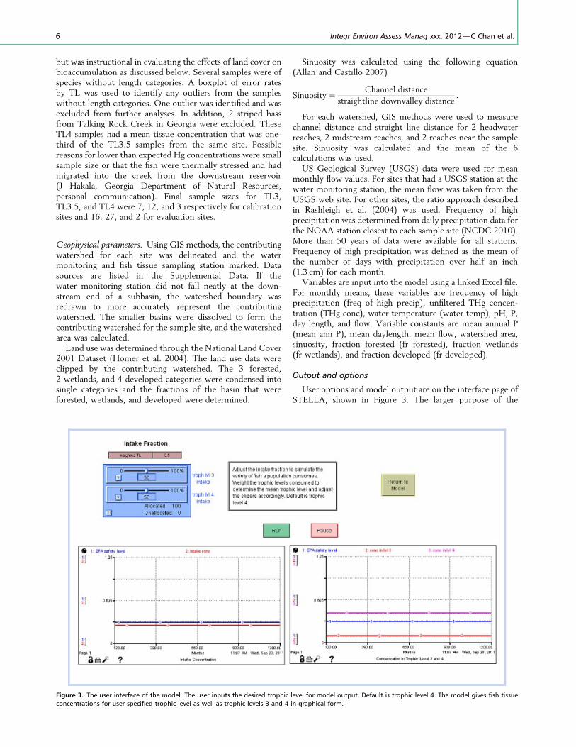
User options and model output are on the interface page ofSTELLA, shown in Figure 3. The larger purpose of the

Figure 3. The user interface of the model. The user inputs the desired trophic level for model output. Default is trophic level 4. The model gives fish tissue

concentrations for user specified trophic level as well as trophic levels 3 and 4 in graphical form.


project is to inform regulatory decision makers on aspects ofthe system that may impact susceptible human populations.Because different populations may consume substantiallydifferent types of fish, the interface contains sliders that theuser sets to simulate the intake TL of the population ofinterest. A numeric display shows this mean TL after theprogram is run. For example, sports fishers are primarilyinterested in piscivorous fish. For that population, the intakeconcentration desired would most likely be TL4. The sliderswould be weighted 100% for TL4. A subsistence fisherpopulation may rely primarily on panfish and catfish. Noslider represents TL3.5, so if 60% of the intake were catfish,weighting would be 30% TL4 and 30% TL3, for catfish. Theremaining 40% of consumption was panfish represented byTL3. Adding this 40%, the final breakdown would be 70%TL3 and 30% TL4. The mean TL consumed would bedisplayed as 3.3.

Output is given in graphical form. TL3 and TL4 are shownon 1 graph and the user designated TL in a separate graph.Because of the complexity of the system, a number of monthsare required for the model to adjust to a steady state conditionbased on individual site factors. To minimize confusion from

this equilibration process, the graphical display begins after asteady state is achieved at 120 months and continues to1200 months for the 100 year run.

CALIBRATION AND EVALUATIONSeven watersheds in Kentucky were chosen to calibrate the

model. Seven basins from outside of Kentucky were chosen toevaluate the model and to determine the limits of modelapplication. All basins were selected based on the availabilityof fish tissue and water quality data. Evaluation basins werefurther limited to sites with similarities to calibration sites inbasin area and wetlands coverage. Locations of calibration andevaluation watersheds are shown in Figure 4, with general sitecharacteristics given in Table 1. More detailed maps showingland cover for calibration and evaluation basins can be foundin the Supplemental Data. The Floyds Fork basin, at 70 km2,was substantially smaller than the other calibration water-sheds, which had areas between 399 and 930 km2. Evalua-tions basins similarly had 1 smaller basin, Spring Creek inGeorgia with an area of 98 km2. The range of the remainingbasins was 220 to 1440 km2.

Figure 4. Locations of calibration and evaluation watersheds. Blue basins were used for model calibration, while those in pink were used to evaluate the model.

See Table 1 for abbreviations of site names.


Natural variability in environmental systems is consider-able. Examination of fish tissue data showed considerablevariability with samples of the same species from the samesite. To compare model output to TL means that, for aparticular site, an understanding of the natural variabilityinherent within a stream system was necessary. The NationalFish Database contains over 100 000 records of Hg in fishtissue from various sources compiled by the USGS (USGSand NIEHS 2006). This database was analyzed to quantify thenatural variability found between fish of the same species ofsimilar size from the same site and collection year. Many ofthese samples were composites of similarly sized fish of thesame species. The data set was analyzed by selecting for themost commonly sampled species that fit within the range of0.75 and 1.25 times the quality length for that species.Selections were further grouped and limited to samples thathad 6 or more of the same species from the same site andcollected the same year. This resulted in 1010 groups. Thestandard deviation was determined for each of these groups,and the mean of these standard deviations was found to be0.116. This mean was used to calculate a 95% confidenceinterval (CI) around the fish tissue means for calibration andevaluation sites. If the calculated lower bound of theconfidence interval was negative, this lower bound was setto 0.

Fit was evaluated by 2 methods; by calculating predictionerror and comparing model output to the 95% CI. Samplemeans, the bounds of the 95% CI, and prediction error areshown in Table 2. Mean error for calibration sites was 26%and 51% for evaluation sites. The model prediction fell withinthe 95% CI for all but 1 of the 20 TL-site combinations. The

site that was outside of these bounds was the MuscatatuckRiver in Indiana. The model prediction was much lower thanthe sample mean. Error for the 2 Indiana sites and TL3 of theLittle Kanawha River in West Virginia was more than twicethat of other evaluation sites. The model prediction was muchlower than the actual samples for all 4 TL-site combinationsin Indiana, but higher for TL3 of the Little Kanawha River.Without these 3 sites, the mean error for the remainingevaluation sites was 26%. Mean error was lowest for TL4 andhighest for TL3 (Table 3).

Land cover varied significantly between basins. Forestedcoverage varied widely whereas wetlands coverage wasminimal to nonexistent for all but 2 basins. Most basins werein rural areas with little development with 1 exception.Regression analyses of land cover fractions compared to errorwere undertaken to evaluate if the model performed moreaccurately based on land cover attributes. No difference wasfound for model accuracy based on land cover (data notshown).

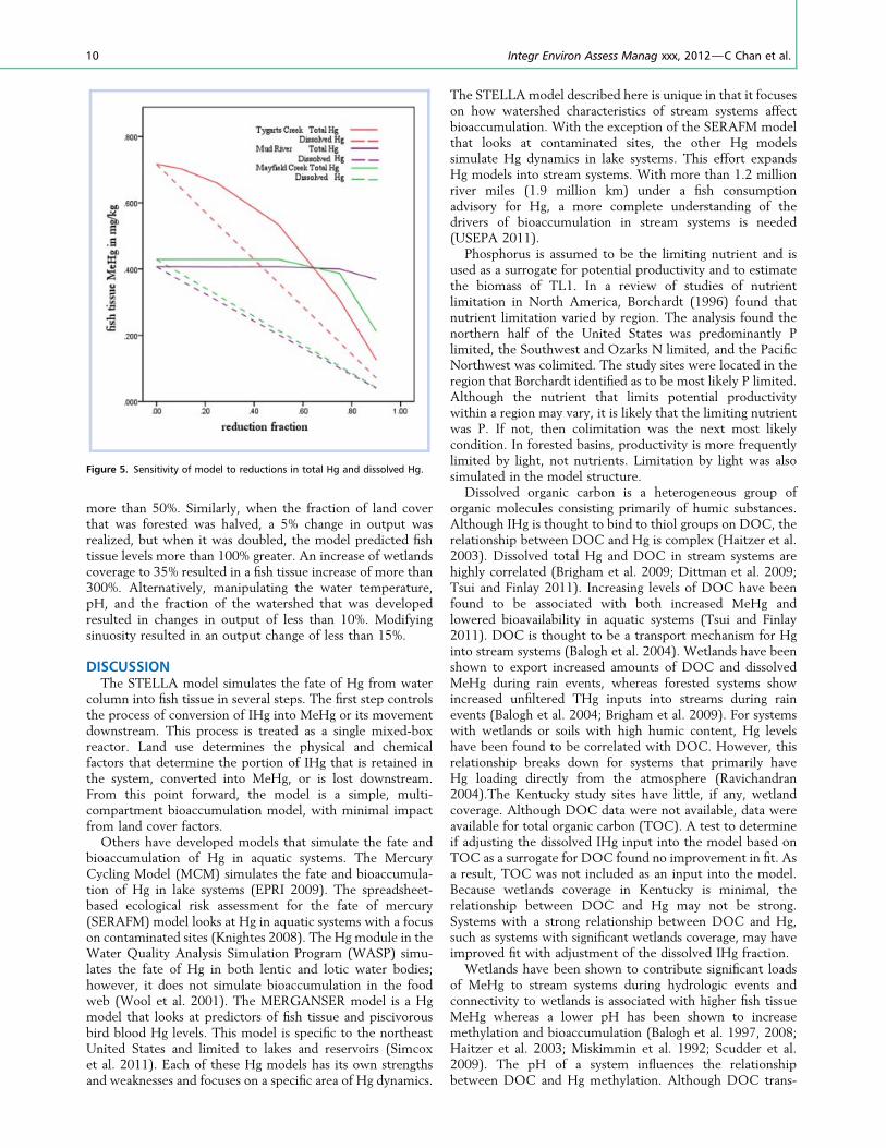
To test the robustness of our model a sensitivity analysiswas carried out. For sensitivity to Hg loading, both unfilteredtotal and dissolved Hg were manipulated for 3 systems with arange of land cover uses. Figure 5 shows the response of fishtissue to percent reductions in both unfiltered total anddissolved Hg for Tygarts Creek, the Mud River, and MayfieldCreek. Reductions in unfiltered THg showed a thresholdeffect in fish tissue levels, whereas reductions in dissolved Hgwere linear.

The sensitivity of the model to other input variables wastested by assessing the impact of manipulating these variables1 at a time within a plausible natural range for 1 of the

Table 1. Site characteristics

SiteSiteabbr

Areakm2

Mean annualQ m3/s

MeanpH

MeanP mg/L

Fractionforested

Fractiondeveloped

Fractionwetlands Sinuosity

Calibration sitesa

Floyds Fork FF 70 1.0 7.79 0.1920 0.359 0.375 0.006 1.81

Mayfield Creek MF 759 12.2 6.96 0.1972 0.234 0.064 0.042 1.00

Mud River MD 689 11.1 7.37 0.0607 0.497 0.059 0.007 2.00

Nolin NL 930 14.1 7.46 0.2139 0.246 0.093 0.000 1.59

Salt River ST 451 7.2 8.03 0.2889 0.244 0.088 0.000 2.13

Slate Creek SE 399 5.7 7.85 0.1005 0.343 0.027 0.000 1.44

Tygarts Creek TG 720 8.8 7.63 0.0193 0.688 0.078 0.000 1.60

Evaluation sites

Big Creek, IN BC 220 2.1 8.06 0.0704 0.099 0.092 0.000 1.48

Little Kanawha River, WV LK 1448 17.0 7.32 0.2085 0.857 0.051 0.000 1.40

Middle Island Creek, WV MI 1282 16.1 7.36 0.2085 0.877 0.046 0.000 1.25

Muscatatuck River, IN MS 733 8.0 8.05 0.1506 0.471 0.050 0.000 1.19

North Fork Forked Deer River, TN FD 448 5.2 6.85 0.2141 0.162 0.077 0.095 1.06

Spring Creek, GA SC 98 1.4 8.07 0.0796 0.477 0.072 0.005 1.21

Talking Rock Creek, GA TR 738 8.1 7.83 0.0441 0.796 0.064 0.003 1.25

aAll calibration sites are in Kentucky. abbr¼ abbreviations; P¼phosphorus; Q¼discharge.


modeled systems. The Mud River site was chosen for thesensitivity analysis because of ample water quality and fishtissue data and land cover and water quality parameters thatwere average compared to the other systems. Parameters thatwere manipulated included the nutrient level, pH, sinuosity,water temperature, and the fractions of land cover that wereforested, wetlands, or developed. Model output in response tothese changes is shown in the Supplemental Data. When Plevels were increased by 300%, model output decreased by10%, but when levels were halved, model output increased by

Table 2. Fish tissue Hg (mg/kg) of sample mean with 95% CI compared to model output and calculated prediction error

Sitea TL Sample

Error calculation

95% CI

Model ErrorLower Upper

Calibration sites

FF 3.5 0.179 0.018 0.340 0.177 0.01

FF 3 0.138 0.000 0.365 0.068 0.51

MD 4 0.366 0.139 0.593 0.430 0.17

MD 3.5 0.176 0.062 0.290 0.260 0.48

MD 3 0.085 0.000 0.186 0.096 0.13

MF 3.5 0.247 0.020 0.474 0.248 0.00

ST 3.5 0.179 0.048 0.310 0.114 0.36

ST 3 0.073 0.000 0.300 0.045 0.38

NL 3.5 0.170 0.000 0.397 0.106 0.38

SE 4 0.190 0.000 0.417 0.217 0.14

Mean 0.26

Evaluation sites

SC 3.5 0.262 0.160 0.364 0.191 0.27

SC 3 0.123 0.009 0.237 0.071 0.42

TR 3.5 0.271 0.195 0.347 0.268 0.01

TR 3 0.065 0.000 0.158 0.076 0.17

BC 3.5 0.260 0.033 0.487 0.057 0.78

BC 3 0.120 0.000 0.281 0.022 0.82

MS 3.5 0.330 0.103 0.557 0.033 0.90

MS 3 0.097 0.000 0.228 0.012 0.88

FD 4 0.426 0.265 0.587 0.355 0.17

FD 3.5 0.162 0.001 0.323 0.217 0.34

LK 3.5 0.174 0.081 0.267 0.096 0.45

LK 3 0.018 0.000 0.245 0.035 0.94

MI 3.5 0.179 0.048 0.310 0.103 0.42

Mean 0.51

aSee Table 1 for site abbreviation information. CI¼ confidence interval; TL¼ trophic level.

Table 3. Prediction error by TL

Sites

TL

3 3.5 4

Calibration 0.34 0.25 0.16

Evaluation 0.65 0.38 0.17

TL¼ trophic level.


more than 50%. Similarly, when the fraction of land coverthat was forested was halved, a 5% change in output wasrealized, but when it was doubled, the model predicted fishtissue levels more than 100% greater. An increase of wetlandscoverage to 35% resulted in a fish tissue increase of more than300%. Alternatively, manipulating the water temperature,pH, and the fraction of the watershed that was developedresulted in changes in output of less than 10%. Modifyingsinuosity resulted in an output change of less than 15%.

DISCUSSIONThe STELLA model simulates the fate of Hg from water

column into fish tissue in several steps. The first step controlsthe process of conversion of IHg into MeHg or its movementdownstream. This process is treated as a single mixed-boxreactor. Land use determines the physical and chemicalfactors that determine the portion of IHg that is retained inthe system, converted into MeHg, or is lost downstream.From this point forward, the model is a simple, multi-compartment bioaccumulation model, with minimal impactfrom land cover factors.

Others have developed models that simulate the fate andbioaccumulation of Hg in aquatic systems. The MercuryCycling Model (MCM) simulates the fate and bioaccumula-tion of Hg in lake systems (EPRI 2009). The spreadsheet-based ecological risk assessment for the fate of mercury(SERAFM) model looks at Hg in aquatic systems with a focuson contaminated sites (Knightes 2008). The Hg module in theWater Quality Analysis Simulation Program (WASP) simu-lates the fate of Hg in both lentic and lotic water bodies;however, it does not simulate bioaccumulation in the foodweb (Wool et al. 2001). The MERGANSER model is a Hgmodel that looks at predictors of fish tissue and piscivorousbird blood Hg levels. This model is specific to the northeastUnited States and limited to lakes and reservoirs (Simcoxet al. 2011). Each of these Hg models has its own strengthsand weaknesses and focuses on a specific area of Hg dynamics.

The STELLA model described here is unique in that it focuseson how watershed characteristics of stream systems affectbioaccumulation. With the exception of the SERAFM modelthat looks at contaminated sites, the other Hg modelssimulate Hg dynamics in lake systems. This effort expandsHg models into stream systems. With more than 1.2 millionriver miles (1.9 million km) under a fish consumptionadvisory for Hg, a more complete understanding of thedrivers of bioaccumulation in stream systems is needed(USEPA 2011).

Phosphorus is assumed to be the limiting nutrient and isused as a surrogate for potential productivity and to estimatethe biomass of TL1. In a review of studies of nutrientlimitation in North America, Borchardt (1996) found thatnutrient limitation varied by region. The analysis found thenorthern half of the United States was predominantly Plimited, the Southwest and Ozarks N limited, and the PacificNorthwest was colimited. The study sites were located in theregion that Borchardt identified as to be most likely P limited.Although the nutrient that limits potential productivitywithin a region may vary, it is likely that the limiting nutrientwas P. If not, then colimitation was the next most likelycondition. In forested basins, productivity is more frequentlylimited by light, not nutrients. Limitation by light was alsosimulated in the model structure.

Dissolved organic carbon is a heterogeneous group oforganic molecules consisting primarily of humic substances.Although IHg is thought to bind to thiol groups on DOC, therelationship between DOC and Hg is complex (Haitzer et al.2003). Dissolved total Hg and DOC in stream systems arehighly correlated (Brigham et al. 2009; Dittman et al. 2009;Tsui and Finlay 2011). Increasing levels of DOC have beenfound to be associated with both increased MeHg andlowered bioavailability in aquatic systems (Tsui and Finlay2011). DOC is thought to be a transport mechanism for Hginto stream systems (Balogh et al. 2004). Wetlands have beenshown to export increased amounts of DOC and dissolvedMeHg during rain events, whereas forested systems showincreased unfiltered THg inputs into streams during rainevents (Balogh et al. 2004; Brigham et al. 2009). For systemswith wetlands or soils with high humic content, Hg levelshave been found to be correlated with DOC. However, thisrelationship breaks down for systems that primarily haveHg loading directly from the atmosphere (Ravichandran2004).The Kentucky study sites have little, if any, wetlandcoverage. Although DOC data were not available, data wereavailable for total organic carbon (TOC). A test to determineif adjusting the dissolved IHg input into the model based onTOC as a surrogate for DOC found no improvement in fit. Asa result, TOC was not included as an input into the model.Because wetlands coverage in Kentucky is minimal, therelationship between DOC and Hg may not be strong.Systems with a strong relationship between DOC and Hg,such as systems with significant wetlands coverage, may haveimproved fit with adjustment of the dissolved IHg fraction.

Wetlands have been shown to contribute significant loadsof MeHg to stream systems during hydrologic events andconnectivity to wetlands is associated with higher fish tissueMeHg whereas a lower pH has been shown to increasemethylation and bioaccumulation (Balogh et al. 1997, 2008;Haitzer et al. 2003; Miskimmin et al. 1992; Scudder et al.2009). The pH of a system influences the relationshipbetween DOC and Hg methylation. Although DOC trans-

Figure 5. Sensitivity of model to reductions in total Hg and dissolved Hg.


ports increased amounts of Hg into stream systems, theavailability of that Hg is dependent on pH. In more acidicsystems, the competition for binding sites from H ionincreases and results in more availability of Hg for methyl-ation (Haitzer et al. 2003). The dissolved IHg input wasadjusted by taking into account the pH of the system,although this adjustment did not improve overall meanprediction error. Calibration sites went from 28% to 26% andevaluation sites from 50% to 51%. However, improvementwas substantial for higher TLs at those few sites with higherwetlands coverage and lower pH. Error for Mayfield Creekdecreased from 36% to 0% for TL3.5. For N. Fork ForkedDeer River, prediction error for TL4 dropped from 46% to17%. Error increased, however, for TL3.5 from 13% to 34% atthat Tennessee site. Because improvement for the systemswith lower pH and higher wetlands coverage was substantial,this adjustment was included in the model as it improvedmodel fit for systems that were not well represented in thisstudy but are likely to be closely looked at by regulators andits inclusion extended the applicability of the model to abroader array of systems.

The minimal variation in wetlands coverage and the smallrange of pHs between the modeled basins are certainlylimitations in the evaluation of the model. Only 2 sites hadwetlands coverage greater than 1% and a mean pH below 7.0.Although the 2 systems with higher wetlands coverage andlower pH had minimal error, more testing is needed to buildconfidence that the model adequately represents the impactof wetlands coverage and pH on bioaccumulation.

Unlike lentic systems, nutrient levels may not be thelimiting factor in primary productivity in stream systems.Light is often limiting for smaller streams. Canopy cover inconjunction with stream width may limit productivity in thestream and consequently be a primary driver for bioaccumu-lation within the biota (Lamberti and Steinman 1997;Vannote et al. 1980). In lower order streams, the canopymay shade the entire stream, and productivity may beminimal after leaf out. As stream order increases, the widthof the stream increases and the canopy opens up resulting inhigher levels of productivity for intermediate sized streams.Larger rivers are deeper and tend to carry more suspendedsolids, both of which reduce light penetration to periphyton-bearing substrates, lowering productivity. Watersheds thatare largely forested have reduced productivity compared tostream systems with abundant light. A reduction in thebiomass of primary producers leads to a higher concentrationof MeHg at the base of the food web. This effect magnifiesthrough the food web, leading to higher fish tissue concen-trations in more pristine settings. The modeled basins weresmall to intermediate in size. Tygarts Creek in particular is asmaller, heavily forested basin. The model predicted thisbasin to have the highest fish tissue concentrations, which wasconfirmed by the collected sample. Although the sample wasbeyond the upper bound of the length range and therefore notincluded in the error analysis, the model predicted thissample, a sauger, to have the highest fish tissue concentrationat 0.708mg/kg. The actual sample was 1.140mg/kg. Qualitylength for sauger is 300mm, and this sample was 432mm.The model does not adjust for length, but the modelprediction supported the expectation that this system wouldhave elevated bioaccumulation.

In the sensitivity analysis, the response to changes in Hgloading differed for total and dissolved Hg. Changes in

unfiltered THg input had little effect on reductions in fishtissue for Mayfield Creek and the Mud River until the amountwas reduced to levels below the 1 ng/L dissolved Hg default.Tygarts Creek, however, showed greater responsiveness tounfiltered THg reductions. Compared to the other 2 systems,Tygarts Creek is more forested, has substantially lessagricultural coverage, and has the lowest mean unfilteredTHg concentrations. Despite having lower unfiltered THgloading, fish tissue levels are highest in this system. In all 3systems, dissolved Hg showed a linear relationship with fishtissue Hg. Balogh et al. (2007) found that in areas with highsuspended solids, unfiltered THg does not correlate to Hg thatis available for microbial conversion (Balogh et al. 1997). Theresponses to reductions in loading of both unfiltered THg anddissolved Hg for these 3 systems support the concept thatmeasures of unfiltered THg do not necessarily correlate withHg available for methylation and that dissolved Hg is a betterpredictor of methylation potential. Although Hg must beavailable for bioaccumulation to occur, basin characteristicsdrive the availability and efficiency with which Hg enters thefood web and bioaccumulates. The sensitivity analysis of Hgloading shows the model accurately simulates the differencesthat basin characteristics impose on Hg availability andbioaccumulation efficiency.

The sensitivity analysis showed that manipulation of pH,and the fraction of land cover that was developed resulted inminimal changes in output. Changes in the nutrient level orthe forested or wetlands coverage, however, had a nontrivialimpact on fish tissue concentrations. Although a lower pHdoes make inorganic Hg more bioavailable (Haitzer et al.2003), this is only 1 factor in determining the mass of Hg thatenters the food web. Development in a basin increases thespeed of transport of Hg through the system, but does notincrease or decrease methylation rates. Although each ofthese variables had some influence on bioaccumulation, thecombination of nutrient levels, and forested and wetlandscoverage of the basin seem to be the strongest driverswithin the modeled systems. The STELLA model allowsthe examination of the impact on bioaccumulation by thestructure of the stream system and reveals the basis for thegreater impact of the most critical variables. These variablesimpact the structure of the system at multiple points.

Nutrient levels and forested coverage are both related toprimary productivity. The relationship between bioaccumu-lation and productivity is complex. Productivity impacts themodel at several points in the system: the calculation of themicrobial conversion rate, the estimate of biomass in thesystem, and the trophic transfer factors. Increased productiv-ity in the form of extensive periphyton mats increases themethylation of Hg, thereby increasing the mass of MeHg inthe biota. Countering this, increased productivity decreasesbioaccumulation through both bloom dilution and somaticgrowth dilution. Hill and Larsen (2005) found that lightlimitation increased the concentration of MeHg in biofilm inartificial streams. Hg uptake was constant under differentlight regimes, but growth of microalgae was dependent onlight. Ward et al. (2010a) studied somatic growth dilution inAtlantic salmon. Fry raised under the same conditions werestocked in various streams and sampled approximately4 months later. Individual growth rate accounted for 38% ofthe variation in Hg concentration in fish tissue, buildingsupport for somatic growth dilution as being an importantfactor in bioaccumulation in stream systems.


The largest impact on bioaccumulation came from landcover factors that influence the amount of IHg in the streamthat is converted into MeHg. Likewise, Chasar et al. (2009)found that, across wide environmental conditions, the supplyof MeHg at the base of the food web was the largest factor toinfluence bioaccumulation, and that trophic structure andtransfer efficiencies were only important predictors whencomparing streams with similar land cover and Hg loading.Riva-Murray et al. (2011) similarly found that MeHg at thebase of the food web was more important than trophicstructure across larger environmental scales. At a smallerscale, they found significant spatial heterogeneity in Hg inbiota within basins that had heterogeneous in-stream habitat.This heterogeneity may be reflecting the different mix offunctional feeding groups. Without having a thorough surveyof the feeding groups in each stream, the proportions for eachstream will be unknown. The assumption is made that thevariation in the composition of functional feeding groups atthe base of the food web is relatively small across the regiondepicted. Bradley et al. (2011) also observed spatial variationin filtered MeHg concentrations in stream reaches corre-sponding to connectivity to wetlands or floodplains orshallow, open-water areas. Smaller reaches may have atypicalland cover and habitat characteristics compared to thecharacteristics of the larger basin containing that reach.Therefore, when using of the model, the size of the basinshould be considered. The model was developed andcalibrated primarily for midsized streams. Use for smaller orlarger basins has not been tested and is likely beyond thecurrent scope of model performance.

Variation within natural settings is large. Stream flow,sunshine and rain, temperature, nutrient levels, growth rates,and other variables fluctuate daily and from year to year. Fishof the same species and size sampled from the same locationwill vary in tissue Hg concentration. A limitation of thismodel is that input parameters inherently have a high degreeof variability, and the use of data collected for regulatorypurposes further compounds the issue. Variable inputs intothe model are monthly or annual means from several years ofmonitoring. Although flow and meteorological data representmany years, water quality data were typically means from 8 or9 years for calibration sites and fewer for evaluation sites. Theassumption in these simulations is that these means representa steady state system. It is not known whether the means fromthese years are typical for these basins over the long term,whether the samples encompass data that are outliers, orwhether there have been recent changes in water quality,weather, or flow. If the assumption of steady state is incorrect,then model output may be biased.

The natural variation between fish tissue samples from thesame species and site limits confidence in the ability toaccurately predict the concentration of Hg in any particularsample. A mean standard deviation of 0.116 was found whenexamining groups of 6 or more samples from the NationalFish Database. When monitoring for regulatory purposes, thenumber of samples are often limited due to the cost ofanalyzing the samples. The combination of considerablevariability and low sample size, even when these are pooledsamples, results in a wide 95% confidence interval. Becauseconfidence intervals are wide, the accuracy of model output ismore difficult to assess. The ultimate purpose of the overallmodel is to gain insight into the complex problem of Hg inthe environment and to understand the factors that control

bioaccumulation and its impact on local susceptible popula-tions. For populations that regularly consume fish from thesame water body, the natural variation between fish willbe averaged, and a mean intake concentration can beconsidered. Regulatory agencies sample fish tissue to deter-mine which waterways present a risk to populations from fishconsumption. At times, agencies have based consumptionadvisories on as few as 1 sample (E Eisiminger, KDOW,personal communication). More frequent and intensivesampling efforts would ensure that an elevated sample wastruly representative of the Hg concentrations in that system.

This model seeks to predict the fish tissue MeHg con-centration in a generic fish species based on TL and basincharacteristics. Accuracy will vary based on the species andsize of fish to which the model output is compared. Whenexamining prediction error by TL at each site, the mean errorfor predicting fish tissue Hg levels was 26% for sites inKentucky and 51% for sites in nearby states. This compareswell with other models that predict fish tissue concentrations.The National Descriptive Model for Mercury in Fish Tissuedeveloped by the USGS reported a prediction error of 38%(Wente 2004). The model developed by Trudel andRasmussen (2006) was within 25% of actual value for 70%of predictions.

One difficulty in developing this model was defining Hgloading to the stream system. Hg was simulated from watercolumn to fish tissue. The model was developed andcalibrated using data from the Kentucky Division of Water,and monthly means of unfiltered THg in the water columnwere used for the input into the system. Soluble Hg isconsidered a more accurate measure of inorganic Hg that isavailable for conversion to MeHg, but dissolved Hg data werenot available. Soluble Hg levels are not always correlated tounfiltered THg levels, especially in systems with highsuspended solids. Measures of DOC, which are more closelyrelated to dissolved Hg levels in stream systems, were notavailable (Brigham et al. 2009). Actual loading is dependenton a number of variables including the amount of precip-itation and the concentration of Hg in that precipitation,the pH of the soil in the watershed, land use, and more. Usingthe monthly mean for Hg loading introduces uncertainty.Spikes of Hg loading, both particulate and dissolved, mayoccur during precipitation events that may not be reflected inmonthly sampling, particularly in basins that may be down-wind of emission sources. Simulating the processes thatinfluence loading into the stream would increase modelaccuracy.

The model was evaluated by comparing model output tofish tissue data for 7 basins in the surrounding region. Themodel was not as accurate at predicting fish tissue concen-trations for evaluation sites. Surprisingly, sites proximal to thestate of Kentucky had higher prediction errors than otherevaluation sites. In particular, the 2 sites in Indiana hadprediction errors ranging from 78% to 90% for the 4 TL-sitecombinations. These sites are in the southeast portion of thestate downwind from a number of coal-fired power plants. Areport by the USGS on Hg in precipitation in Indiana foundthat portion of the state to consistently have the highestHg wet deposition, suggesting that these 2 watersheds maybe located in a Hg hotspot (Risch and Fowler 2008).Hammerschmidt and Fitzgerald (2006) found a positivecorrelation between wet deposition of Hg and MeHgconcentrations in largemouth bass fillets. Gorski et al.


(2008) found that Hg in precipitation was more bioavailablethan Hg in surface waters. The higher loading of dissolved Hgin precipitation may account for the elevated Hg in fishsamples at the Indiana sites compared to model output.Without the Indiana sites, mean prediction error for theevaluation sites was 35%. Adding wet deposition of Hg to themodel might improve model performance. However, wetdeposition data at a spatial scale that is relevant to modelingbasins in the Ohio River Valley are lacking.

In addition to the elevated error at the Indiana sites, TL3 ofthe Little Kanawha River in West Virginia had the highesterror, 94%. This elevated error is misleading. For lower TLs,the magnitude of predicted and actual values are much lower,so differences between those values may result in highererror even though the difference may not be biologicallyrelevant. For the Little Kanawha River, the sample mean was0.018mg/kg and the predicted value was 0.035mg/kgresulting in an error of 94%. If we look at TL3.5 of SpringCreek, the sample mean was 0.262mg/kg and the predictedoutcome was 0.191mg/kg for an error of 27%. The differenceof 0.017mg/kg found at Little Kanawha is biologically lesssignificant than the difference of 0.071mg/kg found at SpringCreek. The error calculations do not convey the biologicalsignificance or magnitude of the error. This scaling of errorvalues at least partially explains the decreasing error withincreasing TL found in Table 3. Mean prediction error forevaluation sites without the Indiana and Little Kanawha siteswas 26%, the same error found for calibration sites.

The basins used to both calibrate and evaluate the modelrepresent a wide variety of geomorphic land types and landuses. In general, the more forested basins were located inmore mountainous areas. Although there was considerablevariability in prediction error between sites, land cover wasnot associated with error. This diversity of land types and usesbuild confidence in the ability of the model to be generalizedto other basins in humid temperate regions with similar basinsize and wetlands coverage.

CONCLUSIONSAs the understanding of the factors that influence bio-

accumulation increases, regulators can begin to predict whichstream systems are most likely to have fish with elevated Hglevels. This knowledge can inform regulatory agencies as towhich stream systems should be given priority for samplingand becomes more important as state budgets become leanerand cost-effectiveness is demanded in all programs. Anunderstanding of watershed factors can also begin to suggestpossible management strategies to reduce bioaccumulation instreams that are out of compliance.

The dynamic bioaccumulation model effectively predictsfish tissue MeHg levels based on watershed characteristics andunfiltered THg concentrations in the water column. Themodel was calibrated and evaluated using 14 diverse basins inor near the Ohio River Valley, a region of North America thatis not well-represented in the Hg bioaccumulation literature.The physiographic diversity and wide span of land usesconvey confidence that the model will predict with reasonableaccuracy fish tissue Hg levels in other similar basins in thetemperate humid domain. Because natural variability in manyof the variables examined in the stream systems is great, moreconsistent and intensive sampling of water quality and fishtissue would improve confidence in model output. If wetdeposition data were available on the scale of the individual

basin, adding this factor might further improve modelaccuracy. Additional evaluation of the model is needed beforesimulating bioaccumulation in basins with significant wet-lands coverage.

The value of this project is that it increases understandingof the interplay of watershed characteristics that impactbioaccumulation in stream systems, particularly in systemswith little wetlands coverage. Wetlands and forested cover-age, and nutrient levels impact Hg dynamics at several pointsin the defined stream system. These parameters appear to bemajor drivers of bioaccumulation for the modeled systems.The model and the insight gained from analyzing variousscenarios can be used by regulatory decision makers to helpdecide which stream systems to test, and to further informthem of the expected responsiveness of a basin to reductionsin Hg loading or possible watershed management strategiesthat could reduce fish tissue Hg levels.

SUPPLEMENTAL DATAModel details and complete documentation. Tables and

land cover maps.Acknowledgment—We thank Jeff Potash for asking the right

questions. Financial support for this project was provided bythe National Institutes of Health Sciences-funded TrainingProgram in Environmental Health Sciences, grant numberT32-ES011564, and STAR Fellowship Assistance Agreementno. FP-91711701-0 awarded by the USEPA. It has not beenformally reviewed by USEPA. The views expressed in thispublication are solely those of the authors, and USEPA doesnot endorse any products or commercial services mentioned inthis publication.

REFERENCESAllan JD, Castillo MM. 2007. Stream ecology: Structure and function of running

waters. Dordrecht, the Netherlands: Springer. 436 p.

Balogh SJ, Meyer ML, Johnson DK. 1997. Mercury and suspended sediment

loadings in the Lower Minnesota River. Environ Sci Technol 31:198–202.

Balogh SJ, Nollet YH, Swain EB. 2004. Redox chemistry inMinnesota streams during

episodes of increased methylmercury discharge. Environ Sci Technol 38:4921–

4927.

Balogh SJ, Swain EB, Nollet YH. 2008. Characteristics of mercury speciation in

Minnesota rivers and streams. Environ Pollut 154:3–11.

Bell AH, Scudder BC. 2007. Mercury accumulation in periphyton of eight river

ecosystems. J Am Water Resour Assoc 43:958–968.

Borchardt M. 1996. Nutrients. In: Stevenson R, Bothwell M, Lowe R, eds. Algal

ecology: Freshwater benthic ecosystems. San Diego, CA: Academic

Press. p 184–228.

Bradley PM, Burns DA, Riva-Murray K, Brigham M, Button DT, Chasar LC, Marvin-

DiPasquale M, Lowery MA, Journey CA. 2011. Spatial and seasonal variability of

dissolved methylmercury in two stream basins in the eastern United States.

Environ Sci Technol 45:2048–2055.

BrighamM,Wentz DA, Aiken GR, Krabbenhoft DP. 2009. Mercury cycling in stream

ecosystems. 1. Water column chemistry and transport. Environ Sci Technol

43:2720–2725.

[CDC] Centers for Disease Control and Prevention. 2004. Blood mercury levels in

young children and childbearing-aged women—United States, 1999–2002.

MMWR Morb Mortal Wkly Rep 53:1018–1020.

Chan C, Heinbokel JF, Myers JA, Jacobs RR. 2011. Development and evaluation of a

dynamic model that projects population biomarkers of methylmercury

exposure from local fish consumption. Integr Environ Assess Manag 7:624–

635.

Chasar LC, Scudder BC, Stewart AR, Bell AH, Aiken GR. 2009. Mercury cycling in

stream ecosystems. 3. Trophic dynamics and methylmercury bioaccumulation.



Chen CY, Folt CL. 2005. High plankton densities reduce mercury biomagnification.


Cleckner LB, Gilmour CC, Hurley JP, Krabbenhoft DP. 1999. Mercury methylation in

periphyton of the Florida Everglades. Limnol Oceanogr 44:1815–1825.

Desrosiers M, Planas D, Mucci A. 2006. Mercury methylation in the epilithon of

Boreal Shield aquatic ecosystems. Environ Sci Technol 40:1540–1546.

Dittman JA, Shanley JB, Driscoll CT, Aiken GR, Chalmers AT, Towse JE. 2009.

Ultraviolet absorbance as a proxy for total dissolved mercury in streams.

Environ Pollut 157:1953–1956.

Emery EB, Spaeth JP. 2011. Mercury concentrations in water and hybrid striped bass

(Morone saxatilis XM. chrysops) muscle tissue samples collected from the Ohio

River, USA. Arch Environ Contam Toxicol 60:486–495.

[EPRI] Electric Power Research Institute. 2009. Dynamic mercury cycling model for

Windows XP/Vista—Amodel for mercury cycling in lakes. D-MCM Version 3.0.

User’s Guide and Technical Reference: EPRI. Palo Alto, CA.

Froese R, Pauly D. Editors. 2011. Fishbase. [cited 2011 November 15] Available

from: www.fishbase.org

Gorski PR, Armstrong DE, Hurley JP, Krabbenhoft DP. 2008. Influence of natural

dissolved organic carbon on the bioavailability of mercury to a freshwater alga.

Environ Pollut 154:116–123.

Haitzer M, Aiken GR, Ryan JN. 2003. Binding of mercury (II) to aquatic humic

substances: Influence of pH and source of humic substances. Environ Sci

Technol 37:2436–2441.

Hammerschmidt CR, Fitzgerald WF. 2006. Methylmercury in freshwater fish linked

to atmospheric mercury deposition. Environ Sci Technol 40:7764–7770.

Harris RC, Rudd JW, Amyot M, Babiarz CL, Beaty KG, Blanchfield PJ, Bodaly RA,

Branfireun BA, Gilmour CC, Graydon JA, et al. 2007. Whole-ecosystem study

shows rapid fish-mercury response to changes in mercury deposition. Proc Natl

Acad Sci U S A 104:16586–16591.

Hill WR, Larsen IL. 2005. Growth dilution of metals in microalgal biofilms. Environ

Sci Technol 39:1513–1518.

Homer , Huang C, Yang L, Wylie B, Coan M. 2004. Development of a 2001 National

Landcover Database for the United States. Photogramm Eng Rem S 70:829–

840.

Karimi R, Chen CY, Pickhardt PC, Fisher NS, Folt CL. 2007. Stoichiometric controls of

mercury dilution by growth. Proc Natl Acad Sci U S A 104:7477–7482.

Knightes CD. 2008. Development and test application of a screening-level mercury

fate model and tool for evaluating wildlife exposure risk for surface waters with

mercury-contaminated sediments (SERAFM). Environ Model Softw 23:495–

510.

Krabbenhoft DP, Wiener JG, Brumbaugh WG, Olson ML, DeWild JF, Sabin TJ. 1999.

A national pilot study of mercury contamination of aquatic ecosystems along

multiple gradients. USGS Investigations Report. Report 99-4018B.

Lamberti GA, Steinman AD. 1997. A comparison of primary production in stream

ecosystems. J N Am Benthol Soc 16:95–104.

Leopold LB. 1994. A view of the river. Cambridge (MA): Harvard University Press.

298 p.

Mauro J, Guimaraes J, Hintelmann H, Watras C, Haack E, Coelho-Souza S. 2002.

Mercury methylation in macrophytes, periphyton, and water—Comparative

studies with stable and radio-mercury additions. Anal Bioanal Chem 374:983–

989.

Miskimmin BM, Rudd JWM, Kelly CA. 1992. Influence of dissolved organic

carbon, pH, and microbial respiration rates on mercury methylation and

demethylation in lake water. Can J Fish Aquat Sci 49:17–22.

[NCDC] National Climatic Data Center. 2010. Climate-radar data inventories. [cited

2011 March 30]. Available from: http://www.ncdc.noaa.gov/oa/climate/

stationlocator.html

Pauly D, Christensen V. 1995. Primary production required to sustain global

fisheries. Nature 374:255–257.

Pickhardt PC, Folt CL, Chen CY, Klaue B, Blum JD. 2002. Algal blooms reduce the

uptake of toxic methylmercury in freshwater food webs. Proc Natl Acad Sci U

S A 99:4419–4423.

Rashleigh B, Barber MC, Cyterski MJ, Johnston JM, Parmar R, Mohamoud Y. 2004.

Population models for stream fish response to habitat and hydrologic

alteration: The CVI Watershed Tool. Research Triangle Park (NC): USEPA.

EPA/600/R-04/190.

Ravichandran M. 2004. Interactions between mercury and dissolved organic

matter—A review. Chemosphere 55:319–331.

Risch MR, Fowler KK. 2008. Mercury in precipitation in Indiana, January 2004-

December 2005. US Geological Survey Scientific Investigations Report. Report

2008-5148.

Riva-Murray K, Chasar LC, Bradley PM, Burns DA, Brigham M, Smith MJ,

Abrahamsen TA. 2011. Spatial patterns of mercury in macroinvertebrates

and fishes from streams of two contrasting forested landscapes in the

eastern United States. Ecotoxicology 20:1530–1542.

Scudder BC, Chasar LC, Wentz DA, Bauch NJ. 2009. Mercury in fish, bed

sediment, and water from streams across the United States, 1998–2005.

US Geological Survey Scientific Investigations Report. Report 2009-

5109.

Shanley JB, Alisa Mast M, Campbell DH, Aiken GR, Krabbenhoft DP, Hunt RJ, Walker

JF, Schuster PF, Chalmers A, Aulenbach BT, et al. 2008. Comparison of total

mercury and methylmercury cycling at five sites using the small watershed

approach. Environ Pollut 154:143–154.

Simcox A, Nacci J, Shanley JB, Johnston JM, Shields L. 2011. MERGANSER—

Predicting mercury levels in fish and loons in New England lakes. EPA

901-F-1-30. Chelmsford, MA, USEPA.

Trudel M, Rasmussen JB. 2006. Bioenergetics and mercury dynamics in fish: A

modelling perspective. Can J Fish Aquat Sci 63:1890–1902.

Tsui MTK, Finlay JC. 2011. Influence of dissolved organic carbon on methylmercury

bioavailability across Minnesota stream ecosystems. Environ Sci Technol

45:5981–5987.

Tsui MTK, Finlay JC, Nater EA. 2009. Mercury bioaccumulation in a stream network.


Tsui MTK, Finlay JC, Balogh SJ, Nollet YH. 2010. In situ production of methylmercury

within a stream channel in northern California. Environ Sci Technol 44:6998–

7004.

[USGS-NIEHS] US Geological Survey and National Institute of Environmental Health

Sciences. 2006. National fish data. [cited 2011 August 11]. Available from:

http://emmma.usgs.gov/datasets.aspx

[USEPA] US Environmental Protection Agency. 1997. Volume III: Fate and transport

of mercury in the environment. USEPA. EPA-452/R-97-005.

[USEPA] US Environmental Protection Agency. 2009. Mercury: Human exposure.

[Cited 2010 March 17. Available from: http://www.epa.gov/mercury/exposure.

htm

[USEPA] US Environmental Protection Agency. 2011. National listing of fish

advisories: Technical fact sheet 2010. [cited 2011 December 19]. Available

from: http://water.epa.gov/scitech/swguidance/fishshellfish/fishadvisories/

technical_factsheet_2010.cfm#figure4

Vannote RL, Minshall GW, Cummins KW, Sedell JR, Cushing CE. 1980. The river

continuum concept. Can J Fish Aquat Sci 37:130–137.

Ward DM, Nislow KH, Chen CY, Folt CL. 2010a. Rapid, efficient growth reduces

mercury concentrations in stream-dwelling Atlantic salmon. Trans Am Fish Soc

139:1–10.

Ward DM, Nislow KH, Folt CL. 2010b. Bioaccumulation syndrome: Identifying

factors that make some stream food webs prone to elevated mercury

bioaccumulation. Ann NY Acad Sci 1195:62–83.

Warner KA, Bonzongo J-CJ, Roden EE, Ward GM, Green AC, Chaubey I, Lyons WB,

Arrington DA. 2005. Effect of watershed parameters on mercury distribution in

different environmental compartments in the Mobile Alabama River Basin,

USA. Sci Total Environ 347:187–207.

Wente SP. 2004. A statistical model and national data set for partitioning fish-tissue

mercury concentration variation between spatiotemporal and sample

characteristic effects. US Geological Survey Scientific Investigation Report.

Report 2004-5199.

White D, Johnston K, Miller M. 2005. Ohio River Basin. In: Benke AC, Cushing CE,

eds. Rivers of North America. Burlington (MA): Elsevier Academic. p 375–

424.

Willis DW, Murphy BR, Guy CS. 1993. Stock density indices: Development, use, and

limitations. Rev Fish Sci 1:203–222.

Wool T, Ambrose RB, Martin J, Comer E. 2001. Water Quality Analysis Simulation

Program (WASP) Version 6. Draft User’s Manual: US Environmental Protection

Agency, Region 4.


A dynamic model using monitoring data and watershed characteristics to project fish tissue mercury...

Documents

Transcript of A dynamic model using monitoring data and watershed characteristics to project fish tissue mercury...