NBER WORKING PAPER SERIES

A DYNAMIC MODEL OF DEMAND FOR HOUSES AND NEIGHBORHOODS

Patrick BayerRobert McMillan

Alvin MurphyChristopher Timmins

Working Paper 17250http://www.nber.org/papers/w17250

NATIONAL BUREAU OF ECONOMIC RESEARCH1050 Massachusetts Avenue

Cambridge, MA 02138July 2011

We would like to thank Morris Davis, Ed Glaeser, Phil Haile, Aviv Nevo, participants at the EconometricSociety Summer Meetings, NBER Summer Institute, Regional Science Annual Meetings, StanfordInstitute for Theoretical Economics, Duke’s Applied Microeconomics lunch groups, and seminar participantsat the University of Arizona, UBC, Georgetown, Minnesota, NYU, Northwestern, Queen’s, Rochester,St. Louis Federal Reserve, and Yale for many helpful comments. We also thank Elliot Anenberg forexcellent research assistance. This research was conducted with the support of the NSF (award #0721136)and SSHRC. All errors are our own. The views expressed herein are those of the authors and do notnecessarily reflect the views of the National Bureau of Economic Research.

© 2011 by Patrick Bayer, Robert McMillan, Alvin Murphy, and Christopher Timmins. All rights reserved.Short sections of text, not to exceed two paragraphs, may be quoted without explicit permission providedthat full credit, including © notice, is given to the source.

A Dynamic Model of Demand for Houses and NeighborhoodsPatrick Bayer, Robert McMillan, Alvin Murphy, and Christopher TimminsNBER Working Paper No. 17250July 2011JEL No. H0,H23,H41,H7,L85,R0,R14,R21,R31,R51

ABSTRACT

We develop a tractable model of neighborhood choice in a dynamic setting along with a computationallystraightforward estimation approach. This approach uses information about neighborhood choicesand the timing of moves to recover moving costs and preferences for dynamically-evolving housingand neighborhood attributes. The model and estimator are potentially applicable to the study of a widerange of dynamic phenomena in housing markets and cities. We focus here on estimating the marginalwillingness to pay for non-marketed amenities – neighborhood racial composition, air pollution, andviolent crime – using rich dynamic data. Consistent with the time-series properties of each amenity,we find that a static demand model understates willingness to pay to avoid pollution and crime butoverstates willingness to pay to live near neighbors of one’s own race. These findings have importantimplications for the class of static housing demand models typically used to value urban amenities.

Patrick BayerDepartment of EconomicsDuke University213 Social SciencesDurham, NC 27708and NBERpatrick.bayer@duke.edu

Robert McMillanUniversity of TorontoDepartment of Economics150 St. George StreetToronto, ON M5S 3G7CANADAand NBERmcmillan@chass.utoronto.ca

Alvin MurphyOlin Business SchoolWashington University in St. LouisBox 1133, 1 Brookings DriveSt. Louis, MO 63130 murphya@wustl.edu

Christopher TimminsDepartment of EconomicsDuke University209 Social Sciences BuildingP.O. Box 90097Durham, NC 27708-0097and NBERchristopher.timmins@duke.edu

1 Introduction

Models of residential sorting1 and hedonic equilibrium2 have been the focus of long

and active literatures in economics. Many well-known theoretical analyses have com-

bined models of individual location decisions with a market-clearing condition to

characterize equilibrium housing prices, household sorting, and public goods provi-

sion in an urban setting. Empirical analyses of these models have also been used

widely, providing estimates of willingness to pay for a variety of non-marketed local

goods (e.g., education, crime, and environmental amenities), estimates of how such

amenities are capitalized into local house prices, and also to simulate the impact of

policy changes on residential sorting and household welfare.3

Despite making progress in many important dimensions, nearly all the models

estimated to date in these literatures have adopted a static approach. This has raised

a concern – shared by critics and practitioners alike4 – that the empirical findings

from estimating static models might be subject to serious biases due to the inherently

dynamic nature of household location decisions.5

That location decisions are dynamic follows from a number of key features of

the housing market: (i) large transactions costs that make moves relatively rare,

(ii) changing household tastes and needs over the life-cycle, and (iii) evolving local

amenities and housing prices that give neighborhoods a dynamic character. Yet

estimating truly dynamic models of the location decision is di!cult for two primary

1Theoretical contributions to this literature include papers by Ellickson (1971), Epple, Filimon,and Romer (1984), Epple and Romer (1991), Epple and Romano (1998), and Nechyba (1999, 2000).Empirical contributions include Epple and Sieg (1999), Ferreyra (2007), Bayer, Ferreira, and McMil-lan (2007), and Kumino! (2008).

2See Rosen (1974), Epple (1987), Ekeland, Heckman, and Nesheim (2004), Bajari and Kahn(2005), Kumino! and Jarrah (2010), Bishop and Timmins (2010) and the papers discussed therein.

3See, for example, Sieg, Smith, Banzhaf, and Walsh (2004), Epple, Romano, and Sieg (2006),and Walsh (2007).

4The dynamic nature of location decisions is often acknowledged by the literature and has, forinstance, prompted a long-standing debate as to whether all households or just recent movers shouldbe used when estimating preferences for amenities. See the discussion in Kahn (1995), Cragg andKahn (1997), or Bayer, Keohane, and Timmins (2009).

5For example, if households know in a dynamic context that an amenity mean-reverts over time,then a static model is likely to understate household valuations of that amenity, as we discuss below.

2

reasons. First, estimation of sorting models generally requires the matching of a large

sample of households along with their characteristics to the features and location of

their housing choices. Given this need, most papers in the previous literature have

used data from the decennial Census, which provides great detail about large cross-

sections of households but very little information about the dynamics of decision-

making or the evolution of households and neighborhoods.6

The second factor that makes estimating dynamic location choice models di!cult

is the high dimensionality of the state space required in order to characterize the

evolution of a system of neighborhoods or cities. Faced with the resulting curse of di-

mensionality, computing a reasonable dynamic model of residential location decisions

that takes account of the heterogeneous and evolving nature of both households and

neighborhoods has proved very challenging. More recently, however, a series of tech-

nical developments in the literature combined with newly available data have made

dynamic estimation in an urban context increasingly feasible.

In this paper, we propose a new method for estimating a dynamic model of de-

mand for houses and neighborhoods. The starting point for our analysis is a unique

data set linking information about buyers and sellers to the universe of housing trans-

actions in the San Francisco metropolitan area over a period of 11 years. In addition

to precise information about housing structure (e.g., square footage, year built, lot

size, transaction price) and house location, a key feature of these data is that they pro-

vide important demographic and economic information about the buyers and sellers

themselves, permitting us to follow households over time when they move house.7

With this data set in hand, we develop a tractable model of neighborhood choice

in a dynamic setting, along with a corresponding estimation approach that is compu-

6Recent papers by Epple, Romano, and Sieg (2010) and Caetano (2010) have made excitingadvances in the estimation of dynamic models by using the limited dynamic information in theCensus in creative ways. By assuming a stationary environment with respect to neighborhood andpopulation evolutions – assumptions that are very reasonable in the context of the questions theyaddress – these papers take important steps forward in studying issues related to household dynamicsover the lifecycle.

7Details of the data matching procedure we use are discussed in the next section.

3

tationally straightforward. This approach, which combines and extends the insights

of Rust (1987), Berry (1994), and Hotz and Miller (1993), allows both the observed

and unobserved features of each neighborhood to evolve over time in a completely

flexible manner. It makes use of information on neighborhood choices and the tim-

ing of moves to recover: (i) preferences for housing and neighborhood attributes,

(ii) preferences for the performance of housing as a financial asset (e.g., expected

appreciation, volatility), and (iii) moving costs.

The model and estimator that we develop build on a number of recent advances

in the industrial organization literature on dynamic demand for durable and storable

goods.8 First, motivated by the fact that housing constitutes two-thirds of the typical

homeowner’s financial portfolio, we explicitly model housing as an asset and allow

each household’s wealth to evolve endogenously. Households in our model anticipate

selling their homes at some point in the future and thus explicitly consider the ex-

pected evolution of neighborhood amenities and housing prices when deciding where

and when to purchase or sell their house.

Second, we develop a novel approach for identifying the marginal utility of con-

sumption, which has long been a thorny issue in the literature on demand estimation

in applications in both industrial organization and urban economics. The main chal-

lenge faced by researchers stems from the strong correlation between a product’s price

and its unobserved quality, generally requiring instruments that are correlated with

price but uncorrelated with unobservables. It is fair to say that such instruments are

hard to come by. In our application, we exploit the fact that households face a mon-

etary trade-o" both in the standard sense of deciding which product (neighborhood)

to purchase but also in the decision of when to move. Here, we take advantage of the

fact that realtor fees during our sample period were quite uniform (6 percent of house

value) in order to identify the marginal utility of consumption when estimating each

resident’s move-stay decision.

Thirdly, we relax the index su!ciency assumption that has become a common

8See Aguirregabiria and Nevo (2010) for an excellent recent review of this literature.

4

feature of the dynamic demand literature. First proposed by Melnikov (2001) and

Hendel and Nevo (2006), this assumption helps to deal with the computational chal-

lenges posed by the large state space typically arising in models of dynamic demand.

Instead of treating the logit inclusive value as a su!cient statistic for predicting fu-

ture continuation values, we construct the continuation value from the underlying

values associated with each neighborhood in the subsequent period, letting those

neighborhood values depend on the current state space in a flexible manner.

We estimate a version of the model that allows for household preference hetero-

geneity on the basis of race, income, and wealth. We then use the estimated utility

parameters to value marginal changes in non-marketed amenities. In particular, we

estimate the way that neighborhood racial composition, violent crime, and air pollu-

tion a"ect the flow utility derived from a particular residential choice.

The findings from this exercise indicate that the preference estimates derived from

our dynamic approach di"er substantially from estimates derived from a compara-

ble static demand model. For example, the per-year willingness to pay to avoid a

10-percent increase in the number violent crimes per 100,000 population is $586 (in

2000 dollars), which is about seventy percent higher than the $344 recovered from a

comparable static estimation procedure. In the case of air pollution, the correspond-

ing di"erences are even larger ($296 from the dynamic model versus $73 from the

static) though still in the same direction. In contrast, the per-year marginal willing-

ness to pay for race (in particular, the preferences of whites for living in proximity

to other whites) is $1,558 whereas the estimate from a naive static model is substan-

tially higher at $1,973. Given the time-series properties of each of these variables, the

sign of the bias from ignoring dynamic considerations accords, in each case, with the

intuition that the valuations of mean-reverting amenities will be understated while

those of positively-persistent amenities will be overstated by a static model.9

9We develop this reasoning more fully in Section 6 below. In the case of a mean-revertingamenity, for example, a static demand model will incorrectly interpret the justifiable downweightingof a high value of the amenity today by households as a low static valuation, thereby understatingwillingness-to-pay for the amenity.

5

Beyond the current application, the model and estimation method that we propose

provide a foundation for addressing a wide set of dynamic issues in housing markets

and cities. These include, for instance, the analysis of the microdynamics of residential

segregation and gentrification within metropolitan areas.10 It is worth noting that

the estimation approach we develop is computationally light, in addition to which the

kinds of transactions data required to estimate the model have become increasingly

available for cities throughout the country in recent years, making further exploration

of these issues very viable.

The remainder of the paper proceeds as follows: Section 2 describes our data set

and the matching procedure used to construct it. Our model, estimation strategy,

and parameter estimates are presented in Sections 3 through 5, respectively. Section

6 discusses the implications of estimating a static demand model when agents are

actually behaving dynamically; and Section 7 concludes.

2 Data

In this section, we describe a new data set that we have assembled, merging infor-

mation about buyers and sellers with the universe of housing transactions in the San

Francisco metropolitan area. We discuss the source data and also demonstrate that

the merge results in a high-quality and representative data set based on multiple

diagnostic tests.

The data set that we construct is drawn from two main sources. The first comes

from Dataquick Information Services, a national real estate data company, and pro-

vides information about each housing unit sold in the core counties of the Bay Area

(San Francisco, Marin, San Mateo, Alameda, Contra Costa, and Santa Clara) be-

tween 1994 and 2004. The buyers’ and sellers’ names are provided, along with the

transaction price, exact street address, square footage, year built, lot size, number of

10Recent theoretical research on aspects of the dynamic microfoundations of housing markets byOrtalo-Magne and Rady (2002, 2006, 2008) and Bajari, Benkard, and Krainer (2005) raise a numberof additional empirical questions that could be addressed using this framework.

6

rooms, number of bathrooms, number of units in building, and many other character-

istics.11 A key feature of this transactions data set is that it also includes information

about the buyer’s mortgage (including the loan amount and lender’s name for all

loans). It is this mortgage information which allows us to link the transactions data

to information about buyers (and many sellers).

The source of the economic and demographic information about buyers and sellers

is the data set on mortgage applications published in accordance with the Home

Mortgage Disclosure Act (HMDA), which was enacted by Congress in 1975 and is

implemented by the Federal Reserve Board’s Regulation C.12 The HMDA data provide

information on the race, income, and gender of the buyer/applicant, as well as the

mortgage loan amount, mortgage lender’s name, and the census tract where the

property is located.

We merge the two data sets on the basis of the following variables: census tract,

loan amount, date, and lender name. Using this procedure, we obtain a unique match

for approximately 70 percent of sales. Because the original transactions data set

includes the full names of buyers and sellers, we are also able to merge demographic

and economic information about sellers into the data set, provided (i) a seller bought

another house within the metropolitan area and (ii) a unique match with HMDA was

obtained for that house. This procedure allows us to merge in information about

sellers for approximately 35-40 percent of our sample.

To ensure that our HMDA/Dataquick matching procedure is valid, we conduct

several diagnostic tests. Using public-access Census micro data from IPUMS, we first

calculate the distributions of income and race of those who purchased a house in

1999 in each of the six Bay Area counties. We compare these distributions to the

11By comparison, the list of housing characteristics is considerably more detailed than that avail-able in Census microdata, for example.

12The purpose of the act is “to provide public loan data that can be used to determine whetherfinancial institutions are serving the housing needs of their communities and whether public o"cialsare distributing public-sector investments so as to attract private investment to areas where itis needed.” Another purpose is to identify any possible discriminatory lending patterns. (Seehttp://www."ec.gov/hmda for more details.)

7

distributions in our merged data set in Table A.1 in the Appendix. As can be seen,

the numbers match almost perfectly in each of the six counties, strongly suggesting

that the matched buyers are representative of all new buyers. Table A.2 provides a

second diagnostic check, concerning the representativeness of the merged data set in

terms of housing characteristics. We report sample statistics for a subset of the house-

level variables taken from the original data set that includes the complete universe

of transactions, as well as sample statistics for the merged data set.13 A comparison

of the two samples suggests that the set of houses for which we have a unique loan

record from HMDA is representative of the universe of houses. Overall, our diagnostic

checks provide strong evidence supporting the validity of our matching procedure.

In addition to merged data on households and the houses they choose, the esti-

mation routine discussed below also requires that we follow households through time

so that we can determine both when they buy and sell a property. Since the data set

provides a complete census of all house sales with a unique code for every property,

it is straightforward to determine if a household moves. And if an individual buys a

house in a given period, we know that he/she will stay there until we see that house

sell again.14

The unit of geography in the model discussed below is a neighborhood, where we

define neighborhoods by merging nearby census tracts until there are approximately

10,000 housing units in each neighborhood.15 We drop a number of neighborhoods

13We drop outlying observations where reported sales price – reported in 2000 dollars – is abovethe 99th or below the 1st percentile of sales prices. We also drop houses with reported values oflot size, square footage, number of bedrooms, and number of rooms higher (or lower) than theirrespective maximum (or minimum) reported in Table A.1.

14More di"cult is determining where a household moves conditional on moving. The raw data donot provide a unique household identifier; however, they do provide the name of both the purchaserand the seller. We use the name information to create a household identifier by looking for a housepurchase in a window of time around a sale for which the purchaser’s name (in the purchase) matchesthe seller’s name (in the sale). If we cannot find a new purchase within a year on either side of thesale, we assume that the household has either left the Bay Area or moved to a rental unit.

15The merging algorithm starts with the least populated census tract, and merges it together withthe nearest tract such that the combined population does not exceed 25,000. The algorithm iteratesuntil no possible combination of tracts would result in combined populations of less than 25,000. Apopulation of 25,000 roughly corresponds to 10,000 housing units. The population and geographicdata for each census tract come from the 2000 Census.

8

that have less than 6 sales in any year between 1994 and 2004,16 leaving us with 225

neighborhoods in total. The corresponding neighborhood boundaries are shown in

Figure 1, along with the county names.

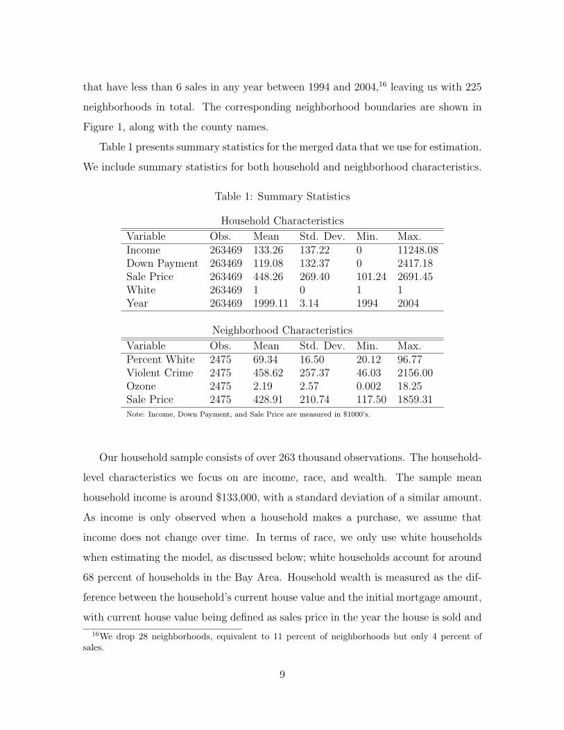
Table 1 presents summary statistics for the merged data that we use for estimation.

We include summary statistics for both household and neighborhood characteristics.

Table 1: Summary Statistics

Household Characteristics

Variable Obs. Mean Std. Dev. Min. Max.Income 263469 133.26 137.22 0 11248.08Down Payment 263469 119.08 132.37 0 2417.18Sale Price 263469 448.26 269.40 101.24 2691.45White 263469 1 0 1 1Year 263469 1999.11 3.14 1994 2004

Neighborhood Characteristics

Variable Obs. Mean Std. Dev. Min. Max.Percent White 2475 69.34 16.50 20.12 96.77Violent Crime 2475 458.62 257.37 46.03 2156.00Ozone 2475 2.19 2.57 0.002 18.25Sale Price 2475 428.91 210.74 117.50 1859.31Note: Income, Down Payment, and Sale Price are measured in $1000’s.

Our household sample consists of over 263 thousand observations. The household-

level characteristics we focus on are income, race, and wealth. The sample mean

household income is around $133,000, with a standard deviation of a similar amount.

As income is only observed when a household makes a purchase, we assume that

income does not change over time. In terms of race, we only use white households

when estimating the model, as discussed below; white households account for around

68 percent of households in the Bay Area. Household wealth is measured as the dif-

ference between the household’s current house value and the initial mortgage amount,

with current house value being defined as sales price in the year the house is sold and

16We drop 28 neighborhoods, equivalent to 11 percent of neighborhoods but only 4 percent ofsales.

9

an imputed price in subsequent years. The imputation uses the original house price

and adjusts this according to an appreciation index generated from a repeat sales

analysis, with the appreciation index calculated separately for each neighborhood.

The neighborhood characteristics we use are mean house price, air quality (ground-

level ozone concentrations), violent crime rates, and the racial composition (per-

centage white) of home owners. We control for changing attributes of the houses

that sold when calculating time variation in each neighborhood’s mean price.17 In

terms of air quality, we use annual data from the California Air Resources Board

(www.arb.ca.gov/adam/) that reports readings from thirty seven monitors in the

Bay Area between 1994-2004. While several di"erent measures of ground-level ozone

pollution are reported in these data, we use information on the number of days each

year that pollution exceeded the one-hour state standard (i.e., 90 parts per billion)

to construct specific measures for each neighborhood centroid. In particular, we use

the latitudes and longitudes of all monitors to construct a distance-weighted average

of the number of ‘exceedances’ for each neighborhood.

Ozone is a convenient environmental disamenity to study in this context. Un-

like many other pollutants, geography and weather are largely responsible for cross-

sectional variation in ground-level ozone pollution. San Francisco, Oakland, and San

Jose all face heavy tra!c congestion. However, wind patterns mitigate much of the

ozone pollution in San Francisco and Oakland, while worsening it in San Jose; and

mountains ringing the southern end of the Bay Area block air flows and contribute to

this e"ect.18 At the same time, fog (which is especially prevalent in San Francisco)

can lower temperatures and block sunlight, preventing the formation of ozone.

In addition to the cross-sectional variation just described, there is also significant

17To generate appreciation trends, we use the same repeat sales analysis used to impute individualhouse values. We regress log price on year and house dummies and create appreciation measuresfrom the coe"cients on the year dummies: the regressions and associated appreciation measures areestimated separately for every neighborhood. This procedure is e!ectively a simplification of themethod described in Case and Shiller (1989). The cross-sectional variation in house prices is drivenby di!erences in prices across neighborhoods averaged over all years.

18The mountains on the eastern side of the Bay are similarly responsible for high levels of pollutionalong the I-680 corridor in eastern Contra Costa and Alameda counties.

10

variation in ozone pollution levels over time, much of which is due to a variety of

programs initiated after California passed its Clean Air Act of 1988. Following several

years of relatively low ozone pollution, the Bay Area experienced its worst year of

air quality for a decade in 1995. In 1996, the vehicle Buyback Program for cars

manufactured in 1975 or before was implemented, and this program contributed to

the summer of 1997 being the cleanest season since the early 1960’s.19 While 1998

saw considerably more ozone pollution, the remaining years of our sample returned to

relatively low levels. There is no reason to expect that any of these programs would

have had special economic consequences for housing prices in any specific part of the

Bay Area, aside from those operating through changing amenity values.

Data on violent crimes are taken from the RAND California data base.20 These

figures represent the number of “crimes against people, including homicide, forcible

rape, robbery, and aggravated assault” per 100,000 residents and are organized by city.

The data describe crime rates for 80 cities in the Bay Area between 1986 and 2008;

and we impute crime rates at the centroid of each neighborhood using a distance-

weighted average of the crime rate in each city. We focus our attention on violent (as

opposed to property) crimes as they are likely to be less subject to reporting error

(see Gibbons (2004)). With that in mind, it is possible that our measure of crime

will, to some extent, proxy for other sorts of crimes as well.

Crime rates in the Bay Area (and in many other parts of the US) fell dramati-

cally over the course of the 1990’s. In the Bay Area, this is particularly evident in

communities starting out with very high rates of violent crime (e.g., East Palo Alto),

whereas low crime areas (e.g., Palo Alto) saw virtually no change in crime rates over

the decade. In general, however, local crime rates have tended to fluctuate in the

short run (annually), and even over longer periods.

The time-series variation in amenities just described may give rise to biases in

static demand estimation, anticipating the application in Section 6. Both ground-level

19Also relevant were the Lawn Mower Buyback and Clean Air Plan of 1997.20http://ca.rand.org/stats/community/crimerate.html

11

ozone and crime vary a great deal from year-to-year and mean-revert over very short

time horizons. Neighborhood racial composition, in contrast, is positively persistent,

with any change in composition today likely to persist into the future. If households

anticipate either the mean reversion or the persistence, their responses will reflect not

only the current change but also those expectations; and as a result, we would expect

a static model to return biased estimates when valuing these amenities. Regressions

exploring the time-series patterns of each (dis)amenity are shown in Table A.3 in the

Appendix.

Figure 1: Appreciation rates by neighborhood

Home Price Appreciation

66% - 75%

76% - 81%

82% - 87%

88% - 92%

93% - 99%

100% - 108%

109% - 121%

122% - 156%

Alameda

Santa Clara

San Mateo

Marin

Contra Costa

San Francisco

The precision of our model depends critically on the fact that rates of change in

amenities and house prices are not uniform across neighborhoods. To illustrate the

variation in the evolution of prices across regions of the Bay Area, Figure 1 shows real

house price appreciation by neighborhood from 1994 to 2004. The estimated price

12

levels are derived separately for each neighborhood using a repeat sales analysis in

which the log of the sales price (in 2000 dollars) is regressed on a set of year fixed

e"ects as well as house fixed e"ects. The figure makes clear the significant di"erences

across neighborhoods in real house price growth over this time period.21

3 A Dynamic Model of Neighborhood Choice

Previous research modeling the process of household sorting across neighborhoods has

generally assumed a static environment.22 In developing a dynamic sorting model, we

introduce the dynamics of the neighborhood choice problem through two channels:

wealth accumulation and moving costs. Households have expectations about the

appreciation of housing prices and may rationally choose a neighborhood that o"ers

lower current period utility in return for the increase in wealth associated with house

price appreciation in that neighborhood. Moving costs are the other component of

the neighborhood choice problem that induce forward-looking behavior. Because

households typically pay six percent of the value of their house in real estate agent

fees, in addition to the non-financial costs of moving, it is prohibitively costly to re-

optimize every period. As a result, households will naturally consider expectations

about future utility streams when deciding where to live, making trade-o"s between

current and future neighborhood attributes and therefore choosing neighborhoods

based in part on demographic or economic trends.

The model we present is one of homeowner behavior.23 Households are treated as

making a sequence of location decisions that maximize the discounted sum of expected

21Omitted neighborhoods in the study area are shaded white, as are the bordering counties.22See Epple and Sieg (1999), Ekeland, Heckman, and Nesheim (2004), Bajari and Kahn (2005),

Ferreyra (2007), and Bayer, McMillan, and Rueben (2011) for several recent examples. Threeexceptions are Kennan and Walker (2011) and Bishop (2007), who analyze interregional migrationin the US in a dynamic context, and Murphy (2007), who examines the role of dynamic behavior inthe supply of new housing.

23We do not explicitly model the decision whether to rent or to own. We do, however, includean outside option that includes moving from home ownership in the Bay Area to either a rentalproperty or a home outside the Bay Area.

13

per-period utilities: formulated in a familiar dynamic programming setup, a Bellman

equation captures the determinants of the optimal choice.

In each period, every household chooses whether or not to move. If a household

moves, it incurs a moving cost and then chooses the neighborhood that yields the

highest expected lifetime utility. The decision variable, di,t, denotes both of the

choices made by household i in period t, namely (i) the decision of whether or not to

move and (ii) the decision of where to move, if the household has decided to move.

If a household decides to move, we denote that decision by di,t = j " {0, 1, . . . , J},

where j indexes neighborhoods, J denotes the total number of neighborhoods in the

Bay Area and 0 denotes the outside option. If a household decides not to move, we

denote this decision by di,t = J + 1.24

The observed state variables at time t are Xj,t, Zi,t, and hi,t. Xj,t is a vector

of characteristics of the di"erent neighborhoods that a"ect the per-period utility a

household may receive from living in neighborhood j " {0, 1, . . . , J}. For example,

Xj,t may include variables such as the price of housing and the quality of local at-

tributes such as air quality, crime, or the neighborhood’s racial composition. Zi,t is a

vector of characteristics of each household that potentially determine the per-period

utility from living in a particular neighborhood, as well as the costs associated with

moving. This vector may include such variables as income, wealth, or race. And

hi,t " {0, 1, . . . , J} denotes the neighborhood chosen in t # 1, including the outside

option.

In addition to the decision variable, di,t, and the observable variables, Xj,t, Zi,t,

and hi,t, there are two unobservable variables, !j,t, and "i,j,t. Of these, !j,t represents

unobserved neighborhood quality,25 and "i,j,t is an idiosyncratic stochastic shock that

24The number of choice options is therefore J+2. For a household who lived in neighborhood j int# 1, we distinguish between the choices of not moving (di,t = J + 1) and of moving to a di!erenthouse within neighborhood j (di,t = j), as there are a small number of observations for whichhouseholds make such within-neighborhood moves. To simplify notation, we do not use a separateindex for neighborhoods and choices. For choices j " {0, 1, . . . , J}, the household is choosing tomove to neighborhood j. For choice j = J + 1, the household is choosing to not move and so toremain in the current neighborhood, which is in {0, 1, . . . , J}.

25We allow households to derive di!erent levels of utility based on their observable demographic

14

determines the utility a household receives from choosing option j " {0, 1, . . . , J +1}

in period t.26 Let si,t denote the states Zi,t, Xt and !t, as well as any other information

set variables, such as lagged characteristics, that help predict future neighborhood or

household characteristics.

The primitives of the model are (u, MC, q, #). Taking these in turn, ui,j,t =

u(Xj,t, !j,t, Zi,t, "i,j,t) is the per-period utility function, excluding any moving costs,

that household i receives from living in neighborhood j. MCi,t = MC(Zi,t, Xhi,t) is

the per-period moving cost function, which is only paid when a household moves. By

assumption, moving costs are not a function of where within the metropolitan area the

household moves to; however, they are assumed to be a function of the characteristics,

Xhi,t , of the neighborhood the household is leaving in order to capture the fact that

realtor fees are proportional to the value of the house one sells. The full flow utility

function is given by uMCi,j,t = ui,j,t # MCi,tI[j !=J+1]. The transition probabilities of

the observables and unobservables are assumed to be Markovian and are given by

q = q(si,t+1, hi,t+1, "i,t+1|si,t, hi,t, "i,t, di,t). Finally, # is the discount factor.

Each household is assumed to behave optimally in the sense that its actions are

taken to maximize lifetime expected utility. That is, the problem of the household is

to make a sequence of residential location decisions, {di,t}, to maximize

E! T"

r=t

#r"t#uMC(Xj,r, !j,r, Zi,r, "i,j,r, Xdi,r!1,r)

$%%si,t, hi,t, "i,t, di,t

&(1)

The optimal decision rule is given by d#, which under the Markov structure of

the problem is only a function of the state variables. That is, di,t = d#i,t(si,t, hi,t, "i,t).

When the sequence of decisions, {di,t}, is determined according to the optimal decision

rule, d#, lifetime expected utility can be represented by the value function. We can

characteristics. In so doing, we di!er from previous work, such as Berry, Levinsohn, and Pakes(1995), that forces all individuals to have the same preferences for the unobserved choice character-istic.

26As the vector of idiosyncratic shocks contains J+2 elements, a household that moves but choosesto reside in the same neighborhood would receive a di!erent draw for ! than if that household chosenot to move.

15

break out the lifetime sum into the flow utility at time t and the expected sum of

flow utilities from time t + 1 onwards. This allows us to use the Bellman equation to

express the value function at time t as the maximum of the sum of flow utility at time

t and the discounted value function at time t+1. We assume that the problem has an

infinite horizon, allowing us to drop the time subscripts on V , the value function:27

V (si,t, hi,t, "i,t) = maxj{uMCi,j,t + #E

!V (si,t+1, hi,t+1, "i,t+1)

%%si,t, hi,t, "i,t, di,t = j&} (2)

Under certain technical assumptions, equation (2) is a contraction mapping in V .

However, the di!culty is that V is a function of both the observed and unobserved

state variables. Therefore, we make a series of assumptions similar to those in Rust

(1987) in order to simplify the model.

Assumption (AS): Additive Separability. We assume that the per-period utility

function, u, is additively separable in the idiosyncratic error term, "i,j,t. Thus we can

express the full flow utility function, uMCi,j,t , as

uMCi,j,t = u(Xj,t, !j,t, Zi,t)#MC(Zi,t, Xhi,t)I[j !=J+1] + "i,j,t (3)

Assumption (CI): Conditional Independence. We make the following assumptions

regarding the transition probabilities of the observed and unobserved states. The

idiosyncratic choice-specific error term, "i,j,t, is distributed i.i.d. Type 1 Extreme

value (with density q!). Additionally, we assume that conditional on si,t and di,t, the

errors "i,j,t have no predictive power regarding future states si,t+1 or hi,t+1. Based on

the structure of the model and the assumption about "i,j,t, it follows that, conditional

on si,t and di,t, the neighborhood chosen in the previous period, hi,t, has no predictive

power regarding any future states and that di,t is su!cient to predict hi,t+1 perfectly.

27Assuming an infinite horizon implies that Vt(si,t, hi,t, !i,t) = V (si,t, hi,t, !i,t) anddt(si,t, hi,t, !i,t) = d(si,t, hi,t, !i,t).

16

We can therefore express the transition density for the Markov process, q, as28

q(si,t+1, hi,t+1, "i,t+1|si,t, hi,t, "i,t, di,t) = qs(si,t+1|si,t, di,t)qh(hi,t+1|di,t)q!("i,t+1) (4)

This allows us to define the choice-specific value function, vMCj (si,t, hi,t), as

vMCj (si,t, hi,t) = ui,j,t#MCi,tI[j !=J+1]+#E

'log

# J+1"

k=0

exp(vMCk (si,t+1, hi,t+1))

$%%%si,t, di,t = j(

(5)

where

log# J+1"

k=1

exp(vMCk (si,t, hi,t))

$= E!

'V (si,t, hi,t, "i,t)

(= E!

'maxk[v

MCk (si,t, hi,t) + "i,k,t]

(

Similarly to per-period utility, we break out the full choice-specific value function

into a component capturing the lifetime expected utility of choosing neighborhood

j ignoring moving costs and another component that involves moving costs. It is

worth noting that the component of lifetime utility that ignores moving costs is not

a function of hi,t, the neighborhood in which the household lives before making the

decision in period t. Thus

vMCj (si,t, hi,t) = vj(si,t)#MC(Zi,t, Xdi,t!1t)I[j !=J+1] (6)

vj(si,t) = ui,j,t + #E'log

# J"

k=0

exp(vMCk (si,t+1, hi,t+1))

$%%%si,t, di,t = j(

(7)

4 Estimation

The estimation of the model primitives proceeds in four stages. In the first stage, we

recover a normalized value of the non-moving cost component of lifetime expected

utility for each neighborhood, time period, and observable household type, where

28In the estimation section, we will outline in detail our assumptions about the transitions of theobservable states.

17

household type is characterized by race, income, and wealth. In the second stage, we

recover moving costs along with an estimate of the marginal value of wealth; the latter

allows us to link the normalized values recovered in the first stage across households

with di"erent wealth levels. We use a novel approach to estimate the marginal value of

wealth in this second stage, utilizing outside information relating to the financial cost

of moving. In the third stage, we recover fully flexible estimates of the per-period

utility. And, with estimates of the per-period utility function in hand, we regress

them on a set of observable attributes in the fourth stage. As will become clear, an

important feature of our estimation strategy is its low computational burden.

4.1 Estimation Stage One – Choice-Specific Value Function

Consider the problem faced by a household that has chosen to move. It will choose a

neighborhood which o"ers the highest lifetime utility by maximizing over the set of

choice-specific value functions vMC . Conditional on moving, the moving cost term,

MC(Zi,t, di,t"1), is assumed to be identical for all neighborhoods. As an additive

constant, it simply drops out and, conditional on moving, each household chooses j

to maximize vj(si,t) + "i,j,t, where vj(si,t) is given in (7).

We have assumed that the idiosyncratic error term, "i,j,t, is distributed i.i.d.,

Type 1 Extreme Value, which allows us to recover vj(si,t) in a number of ways.

Previous methods for estimating dynamic discrete choice models in the presence of

a large choice set are plagued by a curse of dimensionality. We therefore employ a

variant of Hotz and Miller (1993) based on the contraction mapping in Berry (1994),

which avoids this problem. Specifically, based on household characteristics such as

income, wealth, and race, we divide households into distinct types indexed by $ .

Let v"j,t = vj(si,t) when the characteristics (Zi,t) of the household i imply that the

household is of type $ . v"j,t is then a choice-specific value a household of type $

receives from choosing neighborhood j, ignoring any potential moving costs. Letting

u"j,t denote the deterministic component of flow utility for a household of type $ , we

18

can rewrite (7) using lifetime utilities, v"j,t:

v"j,t = u"

j,t + #E'log

) J+1"

k=0

exp(v"t+1

k,t+1 #MC"t+1

j,t+1I[k !=J+1])*%%%si,t, di,t = j

((8)

We assume that agents use the state variables in s and the decision di,t to directly

predict future lifetime utilities, vj,t+1 and future types, $t+1. We discuss exactly how

they forecast in Section 4.3. Household i of type $ chooses choice j if v"j,t + "i,j,t >

v"k,t +"i,k,t, $ k %= j. Conditional upon moving (i.e., for di,t %= J +1), the probability of

any household of type $ choosing neighborhood j in period t when "i,j,t is distributed

i.i.d., Type 1 Extreme Value can therefore be expressed as:

P "j,t(v

"t ) =

ev!j,t

+Jk=0 ev!

k,t(9)

For any given time period, the vector of mean lifetime utilities, v"t , is unique up

to an additive constant, thus requiring some normalization for each $ . Therefore,

instead of recovering v"j,t for every neighborhood and type, we recover v"

j,t, where

v"j,t = v"

j,t#m"t and m"

t is a normalizing constant, a portion of which will be estimated

later in the second step of our estimation procedure. Let P "j,t denote the estimated

probability that households of type $ choose neighborhood j in period t. We can then

easily calculate v"j,t as:

v"j,t = log(P "

j,t)#1

J + 1

J"

k=0

log(P "k,t) (10)

As the number of types, M , grows large relative to the sample size, we may

face some small sample issues with observed shares. Therefore, instead of simply

calculating observed shares as the portion of households of a given type who live in

an area, we use a weighted measure to avoid zero shares. We do this to incorporate

the information from similar types when calculating shares for any particular type.

For example, if we want to calculate the share of households with an income of

19

$50,000 choosing neighborhood j in period t, we would use some information about

the residential decisions of those earning $45,000 or $55,000 in that period. Naturally,

the weights will depend on how far away the other types are in type space. Denoting

the weights by W " (Zi,t), the formula for calculating observed shares (of inside choices)

is given by29

P "j,t =

+Ni=1 I[di,t=j] · W " (Zi,t)+N

i=1 W " (Zi,t)(11)

where the weights are constructed as the product of K kernel weights, where K is

the dimension of Z. Each individual kernel weight is formed using a standard normal

kernel, N , and bandwidth, bk, determined by visual inspection:

W " (Zi,t) =K,

k=1

1

bkN

)Zi,t # Z"

bk

*(12)

We also want to include a lifetime utility term for an outside option. Our data

allow us to follow individuals through time, which means that we can calculate P "0t,

the probability (in each year) that a seller does not buy in the Bay Area. On this

basis, the inside option shares are calculated as the share of those who are buying

(regardless of whether they were previously renting/owning/living in another city)

and who choose neighborhood j. The outside option shares are calculated as the

share of those who were owning in the Bay Area, sell, and then choose to not buy

another house in the Bay Area.30

We use this procedure in combination with the estimated probabilities of choosing

the inside options to obtain a normalized lifetime utility of choosing the outside

options for each type. We denote this lifetime utility as v"0 and include it in the set

of alternatives used in estimating the move/stay decision.

29If W ! (Zi) = I[Zi=Z! ], this results in the simple cells estimator for calculatingshares/probabilities.

30As there are fewer observations for households that we can follow over time, we do not estimatethe outside option shares separately for each year and type. Instead, we include a linear time trendthat is di!erent for each type.

20

4.2 Estimation Stage Two – Moving Costs and the Marginal

Utility of Wealth

In a housing market context, households behave dynamically by taking into account

the e"ect their current decision has on future utility flows. In our model, the current

decision a"ects future utility flows through the two channels mentioned previously

– households are aware that they will incur a transaction cost by re-optimizing in

the future, and in addition, the decision where to live today a"ects wealth in future.

Equation (8) shows how the current decision a"ects both today’s flow utility and

future utility. It also suggests that if v"j,t (or v"

j,t) is known for all $ and j, then

we can estimate moving costs based on households’ decisions to move or stay in a

particular period.

Given that we recover estimates of v"j,t from the first stage, we estimate moving

costs in stage two by considering the move/stay decisions of households in the fol-

lowing way: From the model outlined above, we know that in any given period, a

household will move if the lifetime expected utility of staying in their current neigh-

borhood is less than the lifetime expected utility of the best other alternative when

moving costs are factored in. We assume that moving costs, MC"tj,t, are made up

of two components: financial costs, FMC(hi,t), and psychological costs, PMC(Zi,t).

The financial moving costs are a function of previous location decisions, hi,t, as house-

holds pay financial costs based primarily on the property they sell. The psychological

costs are a function of the observable characteristics, Zi,t, that define type $ .

As the financial moving costs reduce wealth, choosing to move changes a house-

hold’s type. For example, if moving costs are $10,000, then a given household with

$100,000 in wealth chooses where to live based on the utility of staying in their cur-

rent neighborhood with wealth of $100,000 and the highest alternative utility with a

wealth of $90,000. In practice, we treat financial moving costs as observable and set

them equal to 6 percent of the value of housing in the neighborhood that a household

is leaving (i.e., FMC(hi,t) = 0.06 · Pricehi,t).

21

If a household of type $ moves, we denote their new type as $ , the new type

following a move reflecting the reduction in wealth by the amount of FMC. A

household will choose to stay (not move) if:

v"J+1,t + "i,J+1,t > maxk[v

"k,t + "i,k,t]# PMC(Zi,t) (13)

However, from the first stage we only recover the normalized choice-specific value

functions, v"j , where v"

j = v"j #m" . We can then rewrite (13) as:

v"J+1,t + "i,J+1,t > maxk[v

"k,t + "i,k,t]# (m"

t #m"t )# PMC(Zi,t) (14)

The term (m"t #m"

t ) is unobserved but can be estimated as the di"erence between the

value associated with being type $ and the value associated with the reduced wealth

after paying financial moving costs. In principle, we could estimate a separate term

for each combination of $ and FMC; In parctice, we choose to parameterize it as a

function of Zi,t and FMCi,t, so:

m"t #m"

t = FMCi,t%"fmc

where FMCi,t = 0.06 · Pricehi,t and %"fmc = Z $

i,t%fmc. We parameterize the psycho-

logical costs as:

PMCi,t = Z $i,t%pmc

Note that the stochastic terms are maxk !=j[v"k,t + "i,k,t], and "i,J+1,t.31 We estimate

(m"t # m"

t ) and PMCi,t from a likelihood function based on the probability of a

household staying in its current house, where

P "i,t(Stay) =

ev!J+1,t

ev!J+1,t +

+Jk=0 ev!

k,t"FMCi,t#!fmc"Z"

i,t#pmc(15)

31It would be straightforward to also allow for a shock to moving costs, which would e!ectivelyallow all the idiosyncratic errors except !J+1 to be correlated.

22

We then use equation (15) to form a likelihood equation consisting of every house-

hold’s move/stay decision in every period.32 Maximizing this likelihood yields esti-

mates of %fmc and %pmc.

The earlier (first) stage of our estimation approach involved making a normal-

ization for each type of household, where ‘type’ could be defined by personal char-

acteristics such as race, income, and wealth. Once we set the mean choice-specific

utility from having no wealth to zero, we only need to know these baseline di"erences,

m"t # m"

t , in order to recover the unnormalized choice-specific value functions.33 As

we can estimate the baseline di"erences, we simply recover the true choice-specific

value functions as v"j,t = v"

j,t + m"t .

It is important to recover these baseline di"erences because they represent the

additional utility a household would receive from extra wealth, the marginal utility of

wealth being a key output of the estimation. Given that the choice of neighborhood

a"ects future household type, the baseline di"erences in utility across types represent

potential future utility gains from wealth accumulation. In addition, we will also use

the estimate of the marginal value of wealth from this second stage as a novel way to

deal with the endogeneity of house prices in the fourth stage.

4.3 Estimation Stage Three – Per-Period Utility

From stages one and two, we know the distribution of moving costs for each type, the

marginal value of changing type, and the true mean utility terms, v"j . The next step

is to specify and estimate the relevant transition probabilities.

We assume that households use today’s states to directly predict future values of

the lifetime utilities, v, rather than predicting the values of the variables upon which

v depends. As potential future moving costs are a function of the price of housing in

32We assign each household a value, v!j,t, based on which type they are closest to. Alternatively,

we could estimate equation (15) separately for each type using weights similar to those in Stage 1.33We set the mean choice-specific utility from no wealth to zero for each year/income/race com-

bination. However, we are not imposing that these values are identically zero and e!ectively undothis temporary normalization through the use of year*type dummies in Stage 4.

23

the neighborhood chosen in this period, households also need to predict how the price

of the house they currently occupy will transition. Further, as both moving costs and

lifetime utilities are determined by household type, households need to predict how

their types will change. The only determinant of type that changes endogenously

is wealth, so we assume that knowing how house prices transition is su!cient for

knowing how wealth (and therefore type) will transition.34 We therefore only need to

model transition probabilities for v and price.

In theory, we could estimate the transition probabilities for lifetime utility sepa-

rately by type, as we have a time series for each type and neighborhood. However,

to increase the e!ciency of our estimates, we impose some restrictions. Within each

type, we could assume that the neighborhood mean utilities, v"j,t, evolve according to

an auto-regressive process, where some of the coe!cients are common across neigh-

borhoods. In practice, we estimate transition probabilities separately for each type

but pool information over neighborhoods. To account for di"erent means and trends,

we include a separate constant and time trend for each neighborhood’s choice-specific

value function for each type. We model the transition of the choice-specific value

functions, v"j,t, as:

v"j,t = &"

0,j +L"

l=1

&"1,lv

"j,t"l +

L"

l=1

X $j,t"l&

"2,l + &"

3,j t + '"j,t (16)

where the time-varying neighborhood attributes included in Xj,t are price, racial

composition (percentage white), pollution (the number of days that the ozone con-

centration exceeds the California state maximum threshold), and the violent crime

rate.35 Lagged value functions are also included as explanatory variables, implicitly

allowing the transition probabilities be a function of the unobserved neighborhood

attributes.34With access to richer data on other forms of household wealth, the definition of wealth that we

use to define type could be expanded.35For the outside option, we do not observe any attributes and estimate with only lags of the

choice-specific value function. That is, we estimate v!0t = "!

0,0 ++L

l=1 "!1,lv

!0t"l + "!

3,0 t + v!0t.

24

We also need to know how housing wealth transitions in order to specify transition

probabilities for types. We use sales data to construct price indexes for each type-

tract-year combination. Recalling that price is one of the variables in the neighbor-

hood characteristics X, we estimate transition probabilities for price levels according

to:

pricej,t = (0,j +L"

l=1

X $j,t"l(2,l + (3,j t + )"

j,t (17)

Given these transition probabilities, it is straightforward to estimate transition prob-

abilities for wealth and thus type, $ . In both cases, we use two lags of the dependent

variable (v"j,t or price"

j,t) as well as two lags of the other exogenous variables in X.

Knowing v, PMC, and the transition probabilities allows us to calculate mean

flow utilities for each type and neighborhood, u"j,t, according to:

u"j,t = v"

j,t # #E'log

) J+1"

k=0

exp(v"t+1

k,t+1 #MC"t+1

j,t+1I[k !=J+1])*%%%si,t, di,t = j

((18)

where in practice, s includes all the variables on the right hand side of equations (16)

and (17) and # is set equal to 0.95.

For each type, $ , neighborhood, j, and time, t, we now have the necessary in-

formation to simulate the expectation on the right hand side of (18). To do this,

we draw a large number of vt+1’s and pricet+1’s according to their estimated distri-

butions. Specifically, using r to index random draws, each vt+1(r) and pricet+1(r)

are generated by drawing from the empirical distribution of errors obtained when

estimating (16) and (17) and using the observed values of the current states. The

draws on pricet+1 are used to form $t+1 and MC"t+1

j,t+1.36 For each draw, r, we can

then calculate a per-period flow utility u"j,t(r) using (18). The simulated u"

j,t is then

calculated as 1R

+Rr=1 u"

j,t(r).37

36Once we draw a value for pricet+1, we can calculate wealtht+1 for someone living neighborhoodj as wealtht + (pricej,t+1 # pricej,t) and MC!t+1

j,t+1 as 6 percent of pricet+1.37The total number of draws, R, is chosen to be large enough such that the simulated u!

j,t doesnot change as R increases. In practice, setting R equal to 750 is su"cient.

25

4.4 Estimation Stage Four – Decomposing Per-Period Utility

Once we recover the mean per-period flow utilities, we can decompose them into

functions of the observable neighborhood characteristics, Xj,t. We treat !"j,t as an

error term in the following regression:

u"j,t = *"

0 + *"c + *"

t + X $j,t*

"x + !"

j,t (19)

This decomposition of the mean flow utilities is similar to Berry, Levinsohn, and Pakes

(1995) or Bayer, Ferreira, and McMillan (2007), though in these models, the choice-

specific unobservable, !j,t, was treated as a vertical characteristic that a"ected all

households’ utility in the same way. In our application, we allow households who are

di"erent (based on observable demographic characteristics) to view the unobservable

component di"erently, as in Timmins (2007) – hence the $ superscript on !"j,t. The

time-varying characteristics used in our application are the user cost of housing,

ground-level ozone (measured in days exceeding the state standard), violent crime

(measured in incidents per 100,000 residents), and a measure of racial composition

(percentage white). In addition to neighborhood characteristics, we include controls

for type ($), county (c), and year (t).

The user cost of owning a house is typically calculated as a percentage of house

value. Here, we calculate the neighborhood user cost as 5 percent of mean prices in the

neighborhood. User costs are, however, clearly endogenous. The traditional approach

to this problem makes use of instrumental variables. Our approach is di"erent: we

use the marginal value of wealth estimated in Section 4.2 to recover the marginal

disutility of user costs. We assume that the e"ect of a marginal change in wealth on

lifetime utility is the same as the e"ect of a marginal change in income on one period’s

utility. In particular, the marginal utility of income (the negative of which can be

interpreted as the coe!cient on user cost) is given by %"fmc. To decompose mean flow

utilities, we therefore estimate the following regression, where -%"fmc is known from

26

Stage 2 and X denotes the non-user cost components of X:

u"j,t + -%"

fmcusercostj,t = *"0 + *"

c + *"t + X $

j,t*"x + !"

j,t (20)

In principle, we could decompose the flow utilities separately for each type, $ , as

written above. In practice, we constrain some coe!cients to be the same across types

and estimate several di"erent versions of equation (20).

5 Results

We can estimate the model separately for any given time-invariant observable house-

hold characteristic.38 The results we report here are based on estimating the model

for three income types – $40,000, $120,000, and $200,000 – and for whites only.39

In total, we have 75 types: 25 wealth types measured in $10,000 increments – $0 to

$240,000 – interacted with the three income types.

While there are four stages of estimation, the primary results of interest are the

marginal willingness to pay estimates recovered in the final stage. Given our approach

to controlling for the endogeneity of user cost makes use of estimates of the marginal

utility of wealth, we also include a brief discussion of the Stage 2 results.

5.1 Moving Costs and the Marginal Utility of Wealth

We use the binary move/stay decision faced by each household in every period to

identify and estimate the psychological and financial components of moving costs;

using the fact that financial moving costs are 6 percent of the selling price allows us

to recover the marginal value of wealth also. The results of this estimation are given

38As a household’s wealth transitions endogenously, the estimation requires that we include manycategories of wealth.

39The process could be easily replicated for other racial groups, although small-number problemsmay be more of an issue in the first stage for other races. This could be addressed by pooling racialgroups, at least where researchers were not seeking to estimate the value of racial composition byracial group.

27

in Table 2. From the table, it is clear that the psychological costs of moving are large,

they decrease slightly in household income, and are falling over time.40

Table 2: Moving Cost Estimates

Psychological CostsConstant 9.6040

(0.0349)

Income -0.0023(0.00025)

t -0.1092(0.0033)

Financial CostsConstant*6% House Value 0.0323

(0.0012)

Income*6% House Value -0.00009(0.000008)

Note: Income and House Value are measured in $1000’s.

The financial cost estimates are of particular interest, given that they speak to the

marginal value of wealth. These estimates suggest that the marginal value of wealth

is positive but considerably lower for high-income types. The marginal per-period

utility of income coe!cient that we take to the estimation of Stage 4 is given by

0.0323 - 0.00009*income. Our estimate of the marginal per-period utility of income

is decreasing in income, as expected, and is roughly half as small for households with

an income of $200,000 compared to those with an income of $40,000.

40The mean psychological costs are high are they represent the amount a household would pay toavoid moving to a randomly chosen neighborhood in a randomly chosen time period. See Kennanand Walker (2011) for an excellent discussion of the interpretation of moving costs in this class ofmodels.

28

5.2 Marginal Willingness to Pay for Neighborhood Attributes

In the process of decomposing the estimates of flow utilities in the fourth stage, we

control for the endogeneity of user cost by estimating equation (20). We decompose

the flow utilities in two ways. First, we pool the mean utilities for all types and

restrict the preference parameters for percentage white, violent crime, and ozone (as

well as the county and year e"ects) to be same for all households. Later, we relax

these restrictions, estimating willingness to pay separately by income.

The raw coe!cients resulting from this process are di!cult to interpret by them-

selves. Therefore, to better understand the magnitude of the coe!cients, we calculate

per-period willingness to pay for changes in each neighborhood characteristic. Per-

period marginal willingness to pay (in $1000’s) is given by *"x/%

"fmc, which measures

how much a household would be willing to pay annually to receive a small change in

each of the amenities, holding expectations about future amenities constant.

Table 3 reports willingness-to-pay (WTP) measures for a 10-percent change in

each amenity across four di"erent specifications, the WTP figures being given at the

means of percent white (69.34), violent crime rate (458.62), and ozone (2.19). As the

marginal utility of income, %"fmc, varies by income, we report the willingness to pay

measures for a household with income of $120,000, which is close to the mean.

Our preferred specification is reported in column I. In this specification, we exclude

the two highest and two lowest wealth categories and use a Least Absolute Deviations

(LAD) regression to limit the e"ect of outliers. The results show that households with

income of $120,000 are willing to spend $1,558.20 per year to increase percentage

white by ten percent at the mean. The estimates are very precise.41 Analogously,

households with $120,000 in income are willing to pay -$585.56 for a ten-percent

increase in violent crime.42 For ozone, households are willing to pay -$295.60 for

41All the standard errors reported here and elsewhere in the paper were obtained using a bootstrapprocedure with 125 draws.

42This willingness to pay implies a value of a statistical case of violent crime (similar in constructionto the familiar value of a statistical life) of $1.2 million. This amount is consistent with other researchon the costs of crime (Linden and Rocko! (2008)) and is reasonable in magnitude (i.e., approximately

29

a ten-percent increase in the number of days ozone exceeds the threshold.43 To

shed light on the robustness of these WTP estimates, we also estimate the model

using OLS instead of LAD in column II: the results there are quite similar, though

WTP for percent white increases somewhat. In columns III and IV, we estimate

the model without excluding the two highest and two lowest wealth categories using

LAD and OLS regressions, respectively. As can be seen from the table, the results

are reasonably similar to those in column I.

Table 3: Willingness to Pay for a 10-Percent Increase in Amenities

I II III IVPercent White 1558.20 1952.87 1735.40 2270.88

(42.11) (52.78) (46.90) (61.37)

Violent Crime -585.56 -563.69 -603.82 -615.97(15.82) (15.23) (16.32) (16.65)

Ozone -295.60 -329.31 -286.83 -319.76(7.99) (8.90) (7.75) (8.64)

County Dummies Yes Yes Yes YesYear Dummies Yes Yes Yes YesType Dummies Yes Yes Yes YesEstimator LAD OLS LAD OLSWealth Outliers NO NO YES YES

As a supplement to the pooled estimates in Table 3, we also estimate the willingness-

to-pay measures separately for each of the three income types: $40,000, $120,000, and

$200,000. The results are presented in Table 4 and point to significant heterogeneity

in willingness to pay for neighborhood amenities by income. For ease of exposition,

we only show results for our preferred specification – i.e., using median regression and

excluding the extreme wealth types.

The implied income elasticities of demand for neighborhood race are substantial,

16

th the size of a typical VSL estimate).43The corresponding willingness to pay figures for one-unit changes in the three amenities are:

$224.72 per year to increase percentage white by one percentage point, -$12.77 for one additionalviolent crime per 100,000 residents, and -$1,349.77 for one extra day of ozone exceeding the threshold.

30

with a five-fold increase in income raising WTP for percent white almost seven fold.

Similarly for crime, a five-fold increase in income is estimated to increase WTP slightly

more than four fold. In contrast, the implied income elasticities of demand for ozone

are much smaller, with a five fold increase in income only increasing WTP to avoid

ozone by 27 percent.44

Table 4: Willingness to Pay for a 10-Percent Increase in Amenities by Income

$40,000 $120,000 $200,000Percent White 585.35 1342.87 3932.49

(18.36) (36.29) (207.86)

Violent Crime -327.38 -572.33 -1341.25(10.27) (15.47) (70.89)

Ozone -274.62 -292.67 -347.79(8.61) (7.91) (18.38)

6 Dynamic Versus Static Approaches

Equation (8) illustrates the problems associated with estimating a static model when

the true model is dynamic: in essence, specifying a static model creates an omitted

variables problem. In a dynamic setting, current neighborhood characteristics de-

termine the choice-specific value functions in two ways: (i) they a"ect flow utility

directly, and (ii) they help predict future neighborhood utility. Estimating a static

model omits the latter e"ect.

The static model can be conveniently nested within our dynamic framework. The

former e"ectively assumes that the household will always stay in the same location

and that attributes will never change; therefore, the location-specific value function

remains constant over time. As such, one interpretation of the static model is that

44These results are also robust to the alternative specifications shown in Table 3 – available fromthe authors upon request.

31

v"j,t = u"

j,t/(1# #).45 Therefore, the omitted variable can be expressed as:

#E'log

) J+1"

k=0

exp(v"t+1

k,t+1 #MC"t+1

j,t+1I[k !=J+1])*%%%si,t, di,t = j

(# #v"

j,t (21)

The specific way a given current characteristic predicts future utility will determine

whether the static estimator over- or under-predicts the e"ect of that characteristic

on per-period utility. If higher values of a given characteristic predict improvements

in a neighborhood, then the marginal willingness to pay for that attribute will be

biased towards positive infinity, which is the case for all three amenities we consider

(public safety, air quality, and neighborhood percent white).46

To set out the relevant intuition, it is useful to think about the current value of an

attribute predicting future values of that attribute, rather than future utilities. First

consider a disamenity, such as violent crime, that is mean-reverting: as in our data,

a high level of crime today predicts falling crime in future. In this case, we would

expect the static model to understate the disutility of crime. The argument is as

follows: households may be willing to pay quite large amounts to avoid high levels of

crime. However, when they see a neighborhood with high values of this disamenity,

they know that value is likely to fall in the future; and they are therefore willing to

pay much more for a house in that ‘bad’ neighborhood than they would be willing

to pay if the high value of the disamenity were permanent. The upshot is that the

estimated willingness to pay to avoid crime taken from a naive static model will tend

to be biased downward. The same type of argument applies similarly to air pollution

– in our data, ozone levels are also mean-reverting.

There are other neighborhood attributes that are persistent over time, such as

45This interpretation is equivalent to setting # = 0 while making the single-period price equal tothe user cost. The latter is consistent with the literature: no static models of the housing marketassume that the household pays the full sales price for one period’s utility.

46Given that our actual measures are for crime and pollution – disamenities rather than amenities– a positive bias in the relevant coe"cient means that the absolute e!ect of crime and pollutionon utility will be biased downwards – i.e., the static results will suggest households have a weakerdistaste for those disamenities.

32

racial composition. In contrast to ozone and crime, seeing a high percentage of whites

in a neighborhood today signals that the neighborhood is more likely to have an even

higher percentage white in the future. If these are attributes that households value

(and recall that we are only modeling the decisions of white households), they will be

willing to pay more for a house in such a neighborhood than they would if the high

value of the attribute were only temporary – in other words, persistent amenities are

likely to be worth more than fleeting ones. A naive static model ignores this fact and

attributes all of the value to current preferences, thereby overstating the contribution

to flow utility of high percentage white neighborhoods for white households.

To highlight the problems associated with ignoring forward-looking behavior, we

estimate a static version of our model for comparison purposes. Under the assumption

that agents are not forward-looking, a fraction of Stage 1 estimates (i.e., v"j,t(1# #))

can be interpreted as flow utilities. We can then decompose those flow utilities by

running the same Stage 4 procedure used to decompose u"j,t above. In particular,

we estimate equation (20), replacing u"j,t with v"

j,t(1 # #). The marginal utility of

income is recovered in Stage 2 and is still equal to %"fmc. By using the same marginal

utility of income coe!cient as in our dynamic specification, we keep the models as

comparable as possible and limit any bias to the coe!cients on the amenities. Here,

even if the researcher were to incorrectly assume the model to be static, she would

control for the correlation between price and unobserved neighborhood attributes

using an Instrumental Variables approach. Yet if the true model is dynamic, the

chosen instrument will typically not be valid.47

Table 5 reports the marginal willingness to pay for a 10-percent change in each

amenity derived from the static version of the model when we pool all types and

47The problem with the IV strategy is that if the true model is actually dynamic, any staticinstrument will be correlated with expected future utility, which is subsumed in the error term. Inparticular, a condition that any potential instrument must satisfy is that it should be correlated withthe endogenous variable – in this case, price. Now, expected future utility is a function of all currentattributes. Therefore, unless current price has no predictive power with respect to future utility,it will be impossible to find an instrument that is both correlated with price but also uncorrelatedwith expected future utility.

33

evaluate at mean income. The dynamic results from Table 3 are also included for

ease of reference. As before, the marginal willingness to pay figures are reported at

the means of the amenity levels.

Table 5: Willingness to Pay for a 10-Percent Increase in Amenities – Static versusDynamic Estimates

Static DynamicPercent White 1973.79 1558.20

(53.34) (42.11)

Violent Crime -343.63 -585.56(9.29) (15.82)

Ozone -73.25 -295.60(1.98) (7.99)

The comparison of static and dynamic results in the table suggests that incorrectly

estimating a static model in a dynamic context can lead to very biased estimates.

The static model substantially overestimates willingness to pay for living in close

proximity to neighbors of the same race: the static estimate is $1,973.79 whereas

the corresponding dynamic estimate is $1,558.20. The biases for both crime and air

pollution, while also large in absolute terms, run in the opposite direction. The static

estimates for crime are -$343.63 in the static case and -$585.56 in the dynamic case

respectively for a 10-percent increase in violent crime, while for pollution, the static

estimates are -$73.25 versus -$295.60 in the dynamic case, again for a 10-percent

increase in ozone. In each case, the di"erences are substantial and are precisely

estimated.

The signs of these biases are consistent with the discussion above – a high value of

each of the three amenities predicts improvements in the respective neighborhoods.

That is, the partial correlation between the three amenities and the omitted variable,

as defined in equation (21), is positive, meaning that preferences for amenities will be

biased upwards and preferences for disamenities will be biased downwards in absolute

34

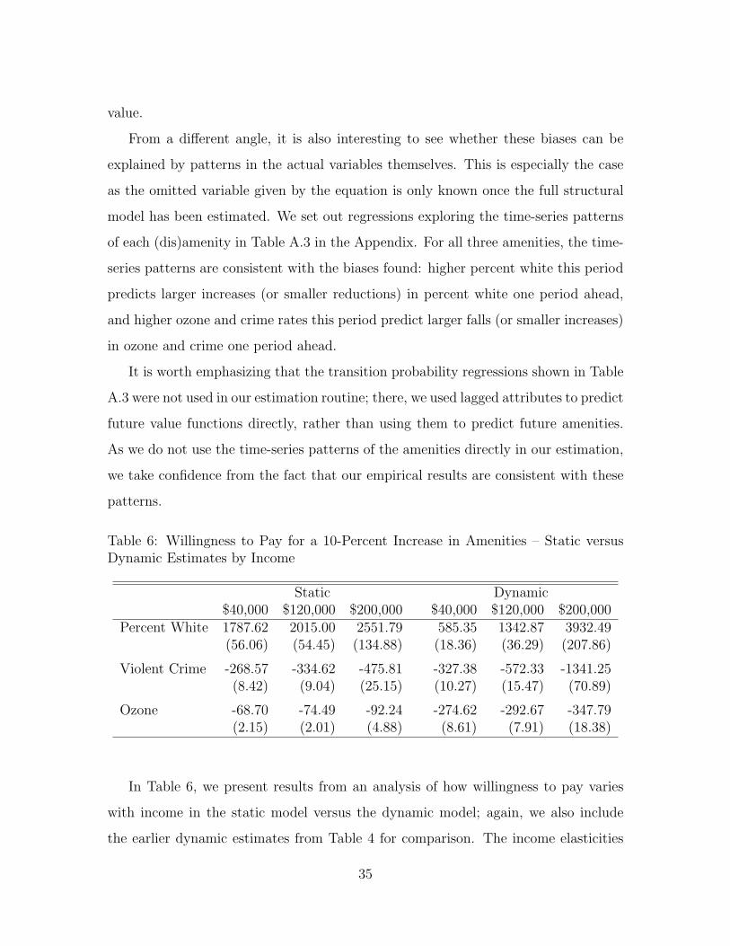
value.

From a di"erent angle, it is also interesting to see whether these biases can be

explained by patterns in the actual variables themselves. This is especially the case

as the omitted variable given by the equation is only known once the full structural

model has been estimated. We set out regressions exploring the time-series patterns

of each (dis)amenity in Table A.3 in the Appendix. For all three amenities, the time-

series patterns are consistent with the biases found: higher percent white this period

predicts larger increases (or smaller reductions) in percent white one period ahead,

and higher ozone and crime rates this period predict larger falls (or smaller increases)

in ozone and crime one period ahead.

It is worth emphasizing that the transition probability regressions shown in Table

A.3 were not used in our estimation routine; there, we used lagged attributes to predict

future value functions directly, rather than using them to predict future amenities.

As we do not use the time-series patterns of the amenities directly in our estimation,

we take confidence from the fact that our empirical results are consistent with these

patterns.

Table 6: Willingness to Pay for a 10-Percent Increase in Amenities – Static versusDynamic Estimates by Income

Static Dynamic$40,000 $120,000 $200,000 $40,000 $120,000 $200,000

Percent White 1787.62 2015.00 2551.79 585.35 1342.87 3932.49(56.06) (54.45) (134.88) (18.36) (36.29) (207.86)

Violent Crime -268.57 -334.62 -475.81 -327.38 -572.33 -1341.25(8.42) (9.04) (25.15) (10.27) (15.47) (70.89)

Ozone -68.70 -74.49 -92.24 -274.62 -292.67 -347.79(2.15) (2.01) (4.88) (8.61) (7.91) (18.38)

In Table 6, we present results from an analysis of how willingness to pay varies

with income in the static model versus the dynamic model; again, we also include

the earlier dynamic estimates from Table 4 for comparison. The income elasticities

35

implied by the static model are substantially smaller for both race and crime relative

to the elasticities from the dynamic model, apparent from the much steeper profiles

in the dynamic case; for ozone, the respective elasticities are fairly similar. The static

model biases are again broadly consistent with the above discussion, with the income

elasticities being considerably larger in the dynamic model, at least for race and crime.

For high-income households, the income elasticity of demand for race is su!ciently

low in the static model that the sign of the bias for high income households changes

direction. All other biases have the same sign in the model where amenity preferences

vary by income type as in the pooled model.48

7 Conclusion

While models of residential sorting and hedonic equilibrium have a long history in

economics, almost all existing empirical studies based on these models have adopted

a static estimation approach. This is with good with reason: computational and

data issues have made the estimation of dynamic models extraordinarily di!cult.

Yet location decisions are inherently dynamic, and this has led to concerns that the

estimates from static models may be seriously biased.

In this paper, we developed a tractable dynamic model of neighborhood choice

that controls for unobserved neighborhood heterogeneity, along with a computation-

ally straightforward semi-parametric estimation approach. Our neighborhood choice

model and estimator adapt dynamic demand models for durable and storable goods

for use in a housing market context, and build on this class of models in several

ways: (i) treating the house as an asset and allowing household wealth to evolve

endogenously, (ii) using stable, uniform realtor fees to estimate the marginal utility

of consumption without the need for a price instrument, and (iii) relaxing the strong

assumption about the evolution of the continuation value that is standard in the

48The patterns described in Tables 5 and 6 are also robust to the alternative specifications shownin Table 3 – available on request.

36

existing literature.

With our model and estimation approach in hand, we merged very rich trans-

actions data with publicly-available mortgage application data to create a data set

that matches the attributes of many buyers and sellers to homes. We then used

this dynamic data set to estimate household preferences in a manner consistent with

forward-looking behavior. In light of the concerns about bias when using static mod-

els, the estimates we obtained indicate that the biases associated with static demand

estimation are significant for three important non-marketed amenities: air quality,

crime, and neighborhood race. Further, the signs of the biases we find are consistent

with what one would expect, based on the time-series properties of each amenity.

Given the importance of accounting for such dynamic considerations when esti-

mating preferences for non-marketed goods, the model, data set, and estimation pro-

cedure presented in this paper have potentially broad applicability to the study of a

range of dynamic phenomena in housing markets and cities. These include examining

the microdynamics of residential segregation and gentrification within metropolitan

areas – applications we intend to pursue in related research using our approach.

37

References

Aguirregabiria, V., and A. Nevo (2010): “Recent Developments in Empiri-

cal Dynamic Models of Demand and Competition in Oligopoly Markets,” mimeo,

University of Toronto.

Bajari, P., C. L. Benkard, and J. Krainer (2005): “House Prices and Con-

sumer Welfare,” Journal of Urban Economics, 58, 474–487.

Bajari, P., and M. Kahn (2005): “Estimating Housing Demand With An Applica-

tion to Explaining Racial Segregation in Cities,” Journal of Business and Economic

Statistics, 23(1), 20–33.

Bayer, P., F. Ferreira, and R. McMillan (2007): “A Unified Framework

for Measuring Preferences for Schools and Neighborhoods,” Journal of Political

Economy, 115(4), 588–638.

Bayer, P., N. Keohane, and C. Timmins (2009): “Migration and Hedonic Val-

uation: The Case of Air Quality,” Journal of Environmental Economics and Man-

agement, 58(1), 1–14.

Bayer, P., R. McMillan, and K. Rueben (2011): “An Equilibrium Model of

Sorting in an Urban Housing Market,” mimeo, Duke University.

Berry, S. (1994): “Estimating Discrete Choice Models of Product Di"eration,”

RAND Journal of Economics, 25, 242–262.

Berry, S., J. Levinsohn, and A. Pakes (1995): “Automobile Prices in Market

Equilibrium,” Econometrica, 63, 841–890.

Bishop, K. (2007): “A Dynamic Model of Location Choice and Hedonic Valuation,”

mimeo, Washington University in St. Louis.

Bishop, K. C., and C. Timmins (2010): “Simple, Consistent Estimation of the

Marginal Willingness to Pay Function: Recovering Rosen’s Second Stage Without

Instrumental Variables,” mimeo, Washington University in St. Louis.

Caetano, G. (2010): “Identification and Estimation of Parental Valuation of School

Quality in the US,” mimeo, University of Rochester.

Case, K., and R. Shiller (1989): “The E!ciency of the Market for Single-Family

Homes,” American Economic Review, 79(1), 125–137.

38

Cragg, M., and M. Kahn (1997): “New Estimates of Climate Demand: Evidence

from Location Choice,” Journal of Urban Economics, 42(2), 261–284.

Ekeland, I., J. J. Heckman, and L. Nesheim (2004): “Identification and Esti-

mation of Hedonic Models,” Journal of Political Economy, 112(1), S60–S109.

Ellickson, B. (1971): “Jurisdictional Fragmentation and Residential Choice,”

American Economic Review, 61(2), 334–339.

Epple, D. (1987): “Hedonic Prices and Implicit Markets: Estimating Demand and

Supply Functions for Di"erentiated Products,” Journal of Political Economy, 95(1),

59–80.

Epple, D., R. Filimon, and T. Romer (1984): “Equilibrium among local juris-

dictions: Toward an integrated treatment of voting and residential choice,” Journal

of Public Economics, 24(3), 281–308.

Epple, D., and R. Romano (1998): “Competition between private and public

schools, vouchers, and peer-group e"ects,” American Economic Review, 88(1), 33–

62.

Epple, D., R. Romano, and H. Sieg (2006): “Admission, Tuition, and Financial

Aid Policies in the Market for Higher Education,” Econometrica, 74(4), 885–928.

(2010): “The Intergenerational Conflict over the Provision of Public Edu-

cation,” mimeo, Carnegie-Mellon University.

Epple, D., and T. Romer (1991): “Mobility and Redistribution,” Journal of Po-

litical Economy, 99(4), 828–858.

Epple, D., and H. Sieg (1999): “Estimating Equilibrium Models of Local Juris-

dictions,” Journal of Political Economy, 107, 645–681.

Ferreyra, M. (2007): “Estimating the E"ects of Private School Vouchers in Multi-

District Economies,” American Economic Review, 97(3), 789–817.

Gibbons, S. (2004): “The Costs of Urban Property Crime,” Economic Journal, 114,

F441–F463.

Hendel, I., and A. Nevo (2006): “Measuring the Implications of Sales and Con-

sumer Inventory Behavior,” Econometrica, 74(6), 1637–1673.

Hotz, V. J., and R. A. Miller (1993): “Conditional Choice Probabilities and the

Estimation of Dynamic Models,” Review of Economic Studies, 60, 497–529.

39

Kahn, M. (1995): “A Revealed Preference Approach to Ranking City Quality of

Life,” Journal of Urban Economics, 38(2), 221–235.

Kennan, J., and J. R. Walker (2011): “The E"ect of Expected Income on Indi-

vidual Migration Decisions,” Econometrica, 79(1), 211–251.

Kuminoff, N. V. (2008): “Recovering Preferences from a Dual-Market Locational

Equilibrium,” mimeo, Arizona State University.

Kuminoff, N. V., and A. S. Jarrah (2010): “A New Approach to Computing

Hedonic Equilibria and Investigating the Properties of Locational Sorting Models,”

Journal of Urban Economics, 67(3), 322–335.

Linden, L., and J. Rockoff (2008): “Estimates of the Impact of Crime Risk on

Property Values from Megan’s Laws,” American Economic Review, 98(3), 1103–

1127.

Melnikov, O. (2001): “Demand for Di"erentiated Durable Products: The Case of

the U.S. Computer Printer Market,” mimeo.

Murphy, A. (2007): “A Dynamic Model of Housing Supply,” mimeo, Washington

University in St. Louis.

Nechyba, T. J. (1999): “School Finance Induced Migration and Stratification Pat-

terns: The Impact of Private School Vouchers,” Journal of Public Economic The-

ory, 1(1), 5–50.

(2000): “Mobility, Targeting, and Private-School Vouchers,” American Eco-

nomic Review, 90(1), 130–146.

Ortalo-Magne, F., and S. Rady (2002): “Tenure Choice and the Riskiness of

Non-Housing Consumption,” Journal of Housing Economics, 11(3), 266–279.

(2006): “Housing Market Dynamics: On the Contribution of Income Shocks

and Credit Constraints,” Review of Economic Studies, 73(2), 459–485.

(2008): “Heterogeneity Within Communities: A Stochastic Model with

Tenure Choice,” Journal of Urban Economics, 64(1), 1–17.

Rosen, S. (1974): “Hedonic Prices and Implicit Markets: Product Di"erentiation in

Pure Competition,” Journal of Political Economy, 82(1), 34–55.

Rust, J. (1987): “Optimal Replacement of GMC Bus Engines: An Empirical Model

of Harold Zurcher,” Econometrica, 55(5), 999–1033.

40

Sieg, H., V. K. Smith, H. S. Banzhaf, and R. Walsh (2004): “Estimating

the General Equilibrium Benefits of Large Changes in Spatially Delineated Public

Goods,” International Economic Review, 45, 1047–1077.

Timmins, C. (2007): “If You Can’t Take the Heat, Get Out of the Cerrado... Recov-

ering the Equilibrium Amenity Cost of Non-Marginal Climate Change in Brazil,”

Journal of Regional Science, 47(1), 1–25.

Walsh, R. (2007): “Endogenous Open Space Amenities in a Locational Equilib-

rium,” Journal of Urban Economics, 61(2), 319–344.

41

Appendix

Table A.1: Comparison of Sample Statistics for Merged Data and IPUMS Data byBay Area County

ALAM C.C. MARIN S.F. S.M. S.C.

HMDA / Transactions DataMedian Income 83000 78000 121000 103000 108000 101000Mean Income 98977 99141 166220 147019 137777 123138Std Dev Income 96319 97928 176660 225646 123762 125138

IPUMSMedian Income 83400 76785 120000 100000 102400 100000Mean Income 104167 99047 162322 137555 140447 124483Std Dev Income 84823 83932 138329 121552 123451 99373

HMDA / Transactions DataPercent White 49.85 68.27 90.65 59.12 60.08 49.07Percent Asian 28.68 10.55 4.68 31.47 26.57 34.21Percent Black 6.45 6.01 0.67 2.08 1.22 1.45Percent Hispanic 11.76 12.38 2.51 5.86 9.90 12.27

IPUMSPercent White 47.64 64.57 87.5 61.92 58.1 50Percent Asian 27.34 11.37 3.3 23.37 25.41 33.51Percent Black 7.77 6.05 2.3 2.8 1.24 1.16Percent Hispanic 14.62 14.2 3.62 8.18 12.5 12.09

42

Table A.2: Comparison of Sample Statistics for Transactions Data and Merged Data

Transactions Data

Variable Obs. Mean Std. Dev. Min. Max.Sale Price 1045920 354915 220886 16500 1521333Lot Size 1045920 6857 11197 0 199940Square Footage 1045920 1647 714 400 10000Number Bedrooms 1045920 2.98 1.10 0 8Number Rooms 1045920 6.73 2.00 1 18

Merged HMDA/Transactions Data

Variable Obs. Mean Std. Dev. Min. Max.Sale Price 804699 372240 212938 16513 1521204Lot Size 804699 6730 10605 0 199940Square Footage 804699 1649 687 400 10000Number Bedrooms 804699 3.01 1.08 0 8Number Rooms 804699 6.77 1.98 1 18

Table A.3: Time-Series Properties of Amenities

# Percent Whitet+1 # Violent Crimet+1 # Ozonet+1

Percent Whitet 0.0162 -0.3736 0.0097(0.0002) (0.0138) (0.0003)

Violent Crimet 0.0010 -0.1605 -0.0010(0.00001) (0.0010) (0.00002)

Ozonet -0.01185 -1.2256 -0.6578(0.0014) (0.1034) (0.0021)

County Dummies Yes Yes YesYear Dummies Yes Yes YesNote: For the dependent variable, !Xt+1 = Xt+1 " Xt.

43