Working Paper Researchby Marina Emiris

November 2016 No 313

A dynamic factor model for forecasting house prices in Belgium

NBB WORKING PAPER No. 313 – NOVEMBER 2016

Editor Jan Smets, Governor of the National Bank of Belgium Statement of purpose:

The purpose of these working papers is to promote the circulation of research results (Research Series) and analytical studies (Documents Series) made within the National Bank of Belgium or presented by external economists in seminars, conferences and conventions organised by the Bank. The aim is therefore to provide a platform for discussion. The opinions expressed are strictly those of the authors and do not necessarily reflect the views of the National Bank of Belgium. Orders

For orders and information on subscriptions and reductions: National Bank of Belgium, Documentation - Publications service, boulevard de Berlaimont 14, 1000 Brussels Tel +32 2 221 20 33 - Fax +32 2 21 30 42 The Working Papers are available on the website of the Bank: http://www.nbb.be © National Bank of Belgium, Brussels All rights reserved. Reproduction for educational and non-commercial purposes is permitted provided that the source is acknowledged. ISSN: 1375-680X (print) ISSN: 1784-2476 (online)

NBB WORKING PAPER No. 313 – NOVEMBER 2016

Abstract The paper forecasts the residential property price index in Belgium with a dynamic factor model

(DFM) estimated with a dataset of macro-economic variables describing the Belgian and euro area

economy. The model is validated with out-of-sample forecasts which are obtained recursively over

an expanding window over the period 2000q1-2012q4. We illustrate how the model reads

information from mortgage loans, interest rates, GDP and inflation to revise the residential property

price forecast as a result of a change in assumptions for the future paths of these variables.

JEL classification: E32, G21, C53

Keywords: dynamic factor model, conditional forecast, house prices Author Marina Emiris, Economics and Research Department, National Bank of Belgium, e-mail:

marina.emiris@nbb.be. Acknowledgements I would like to thank D. Antonio Liedo, R. Wouters, and C. Fuss for their comments and suggestions. The views expressed in this paper are those of the author and do not necessarily reflect the views of the National Bank of Belgium or any other institution to which the author are affiliated. All remaining errors are our own.

NBB WORKING PAPER - No. 313 – NOVEMBER 2016

TABLE OF CONTENTS

1. Introduction ....................................................................................................................... 1 2. Modelling Approach .......................................................................................................... 5

2.1. Model ................................................................................................................................... 5

2.2. Estimation ............................................................................................................................ 8

3. Empirical Results ............................................................................................................. 10 3.1. Data ................................................................................................................................... 11

3.2. Model specification ............................................................................................................. 13

3.3. Forecasting ........................................................................................................................ 14

3.3.1. Model validation – Recursive Out-of-Sample Unconditional and Conditional

Forecasts............................................................................................................... 14

3.4. Accounting for Revisions in the Residential Property Price Forecast in Terms of

Changes in the Conditioning Assumptions .......................................................................... 18

3.4.1. House prices up to 2007 and a summary of the 2007 and 2008 scenarios .............. 19

3.4.2. The residential property price forecast and the impact of the change in the

macroeconomic environment ................................................................................. 21

4. Conclusion ....................................................................................................................... 23

References ................................................................................................................................. 25

Appendix ..................................................................................................................................... 28

Tables.......................................................................................................................................... 31

Figures ........................................................................................................................................ 35

National Bank of Belgium - Working papers series ...................................................................... 47

1 Introduction

The aim of this paper is to compute real house price forecasts that are com-

patible with the evolution of macroeconomic variables in Belgium and the euro

area. This type of forecast is widely used in several contexts in central banks as

the outlook for residential property prices helps assess the state of the macro-

economy and �nancial stability. For example, national central banks in the euro

area are required to send in forecasts to the ECB on the likely path of a national

index of residential property prices over a horizon of 12 quarters as part of the

macroeconomic projection exercises in June and in December each year. The

outlook for house prices is also used as an input for bank stress-testing.

House prices, along with other �nancial indicators, move jointly with fu-

ture economic activity and in�ation. The recent �nancial crisis, as well as its

links with the housing market boom and bust in several countries around the

world, has provided additional evidence that housing variables comove strongly

with the business cycle (Heathcote and Davis (2005), Leamer (2007), Case and

Wachter (2005), Girouard et.al (2006)). House price busts accompanied by

credit contractions have been shown to precede longer and deeper recessions

(Claessens, Cose and Terrones (2008)). Recent research also has focused on

the feedback mechanisms between housing markets and the economy, investi-

gating for example the role of monetary policy in fuelling or preventing a house

price bubble (Luciani (2013), Jarocinski and Smets (2008)), and studying the

"housing cycle" and spillovers from housing to consumption before and after

the �nancial crisis.

This paper acknowledges these complex interactions between the housing

market and the rest of the economy by proposing a joint model for residential

property prices and a large number of indicators that are relevant to charac-

terise the Belgian economy, including its external environment. The paper has

a twofold objective. First, to jointly forecast residential property prices and

the economy in Belgium. Second, to use this framework to impose alternative

scenarios on the path of some variables, such as interest rates, and to deduce

1

the conditional forecasts or the paths for the residential property price index

that are consistent with these scenarios. The modelling approach followed in

this paper borrows from the literature on dynamic factor models. The aim is to

extract the key driving factors from a large information set of macroeconomic

variables in Belgium and the euro area in a parsimonious manner in order to

ensure their usefulness for out-of-sample forecasting.

The dynamic factor model exploits the fact that the residential property price

index, interest rates and other macroeconomic and �nancial variables comove

strongly. In its simplest form, any series is modelled as a sum of two com-

ponents: a "common component", which is driven by an unobserved common

factor (for example "the business cycle") and produces the observed correlation

of the residential property price index with the other series; an "idiosyncratic

component", which is uncorrelated with the common component and is speci�c

to each of the series and uncorrelated from the other idiosyncratic components.

The factors are dynamic, in the sense they are driven by a few common shocks

that propagate across variables and in time through the factors themselves.

By making the assumption that there is only a small number of unobserved

common sources producing the observed comovement of the di¤erent time series,

the dynamic factor model o¤ers a parsimonious representation of each variable

in the dataset. It maps the information from all the variables into a few factors

and implies that the number of parameters to estimate remains small as we add

variables to the dataset (see Stock and Watson (2011)).

This assumption is too restrictive in large datasets. For example, in large

datasets of macroeconomic variables, the idiosyncratic component for series that

are similar in nature ("prices", grouping such variables as a consumer price in-

dex, GDP de�ator, etc. or "real variables" grouping GDP and its components,

consumption, investment etc.) or variables concerning the same geographi-

cal area, are bound to be correlated even after we control for a few common

economy-wide factors. We deal with this problem by incorporating several fac-

tors in each block of variables in such a way that the residual cross-correlation

patterns can be considered idiosyncratic or at least weakly correlated across

2

variables1 .

Although there is a large literature on modelling and explaining house prices,

few papers focus speci�cally on forecasting. The most widely used empirical ap-

proach is based on an inverted demand equation. The supply of housing services

is assumed to be relatively inelastic in the short run and it is mainly changes

in demand that explain variation in house prices. In this context, housing is

treated as a consumption good and its demand is a function of such variables

as household income, interest rates, the mortgage rate, �nancial wealth, demo-

graphic and labour market factors. This approach links the level of house prices

to its short-run and long-run determinants in an error correction model (ECM)

or a vector error correction model (VECM). Changes in house prices are a func-

tion of changes in the explanatory variables and an error-correction term which

re�ects the adjustment of house prices to a disequilibrium. An example of this

approach is given by Gattini and Hiebert (2010) for the euro area.

These models are mainly used to determine any over/undervaluation of house

prices as a deviation from the values implied by a long-run equilibrium. Al-

though VECMs have been used for forecasting, other types of models that allow

for more �exibility in their parameters should outperform the VECM forecasts.

For example, Bayesian vector autoregressions (BVARs) should perform better.

Examples in the literature of BVARs with house prices, residential investment

along with other macroeconomic variables are Jarocinski and Smets (2008), Ia-

coviello and Neri (2010). These papers model the level of house prices along

with other macroeconomic and �nancial determinants. BVARs have been used

in combination with structural theoretical models to impose restrictions on the

BVAR parameters stemming from a theoretical dynamic stochastic general equi-

librium model (DSGE). However, in these papers, the focus is not so much on

1The literature on so-called "approximate" dynamic factor models has shown that even if

the data-generating process has locally, or mildly correlated idiosyncratic components, it is

still possible to estimate the parameters of the above dynamic factor model in a consistent way

(see Forni, Hallin Lippi, and Reichlin (2000); Stock and Watson (2002), Bai and Ng (2002);

Bai (2003); Forni, Hallin, Lippi and Reichlin (2004); Doz, Giannone and Reichlin (2012)).

3

forecasting as it is on explaining the interactions of house prices / the housing

sector and the economy and �nding empirical support for the proposed DSGE

model.

Similarly, models that make it possible to increase the number of vari-

ables included in the dataset such as factor-augmented vector auto-regressions

(FAVARs), as in Eickmeirer and Hofmann (2013), or structural dynamic factor

models, as in Luciani (2013), have modelled house prices and their interactions

with the economy in a structural context, seeking to understand the role of

monetary policy and credit in fuelling the house price bubble in the US during

the period 2000-2006.

The focus of our paper is on forecasting house prices. Therefore, the dynamic

factor model will be estimated in reduced form, without imposing any identifying

restrictions on the parameters, so as to give it as much �exibility as possible

to maximise its forecast performance. The link with a structural model can

be achieved in a subsequent step by identifying the shocks as in the structural

models, even though this task will not be undertaken in this paper.

The model will be written in state space form and estimated by (quasi-)

maximum likelihood following Doz, Giannone and Reichlin (2012). The estima-

tion procedure is based on the expectation-maximisation (EM) algorithm and a

Kalman �lter/smoother which jointly estimates the factors, the factor dynamics

and the loadings of the variables on the factors. The advantage of the state-

space approach is the possibility to recursively obtain forecasts conditional on

assumptions on the evolution of a block of variables of interest.

First, the parameters and the factors are estimated over a given sample.

Then, residential property prices are forecast over di¤erent horizons in two ways.

In the �rst part of the empirical section, we use the �nal data realisations, as

available in 2013q3, thereby ignoring data revisions. We start with an out-of-

sample experiment where unconditional forecasts for house prices are recursively

calculated using a balanced panel. Then, we assess the extent to which those

house price forecasts for a given period would have improved had we made them

conditional on data, up to that period, for a block of variables such as mortgage

4

loans, interest rates, the GDP and in�ation rate. Thus, in this �rst exercise, the

conditioning information refers to actual data. This experiment is designed to

answer the question: "Had the actual data on the macroeconomic environment

been ´revealed ´ to us at the time of the forecast (and before it was actually

published) and had it been exploited by the model, would the forecast have

improved relative to the forecast obtained without this information?". This

particular out-of-sample forecasting exercise is important to understand the

second part of our empirical application, in which the conditioning information

is taken from expectations, published in the NBB Economic Review, regarding

those series over the forecasting horizon.

In the second part of the empirical section of the paper, we apply this fore-

casting methodology to account for the revisions in real house price forecasts

in terms of changes in the conditioning assumptions. We produce forecasts for

the residential property price index at two points in time. The �rst time is in

September 2007 given the assumptions for the December 2007 macroeconomic

projection exercise and then, one year later, given the new assumptions for

the December 2008 macroeconomic projection exercise. When a new scenario

becomes available, the conditional forecast is updated and a new conditional

forecast can be derived. The update is broken down into several components,

each tracing back to the variable whose path changed under the new scenario.

The next section focuses on the modelling approach. In the third section, we

describe the data, estimate and validate the model and forecast the residential

property price index. The �nal section concludes.

2 Modelling Approach

2.1 Model

All variables yit(i = 1:::n) in the dataset are jointly represented by a dynamic

factor model. The idea is that all the variables, both those that describe the

macroeconomic environment in Belgium, and those that describe the housing

5

market and the external environment have common dynamics which are gen-

erated by a few common shocks wt, such as monetary policy, that propagate

to the common factors ft (a common underlying "business cycle" for example)

and to the observable variables.

The dynamic factor model decomposes any stationary observable variable in

the dataset, fyitg ; t = 1:::T;measured in quarters, into a component �0

ift driven

by r shocks ut common to all variables and a component eit that is speci�c to

that particular variable i and uncorrelated from all other ejt; j 6= i and its past

eit�1; :::; eit�p:

The vector yt = [y1t; y2t; :::; ynt]0; t = 1; :::T that groups the variables is a

stationary n�dimensional vector process. Each variable is standardised with

mean 0 and unit variance2 and yt has the following dynamic factor model

representation:

yt = �ft + et; et � N(0; R) (1)

ft = A1ft�1 + :::+Apft�p + ut (2)

ut = Bwt wt � N(0; Ir)

E[etw0

t] = 0

where ft is a r � 1 vector of unobserved stationary common factors and et =

(e1t; :::; ent)0 is the idiosyncratic component. R is assumed to be diagonal. This

implies that the factor model is exact; all the dynamic interactions between the

observable variables can be attributed to the r factors.

The r factors are modelled as a stationary vector autoregressive process of

order p, where A1; :::; Ap are r � r matrices of autoregressive coe¢ cients; the

common shocks ujt , j = 1::r and the idiosyncratic components eit are normally

2Stationarity is obtained by taking log-di¤erences of the non-stationary variables in lev-

els. The variables are standardised before estimation by substracting their sample mean and

dividing by their sample standard deviation. The variables are re-scaled at the end of the

estimation process. More details on the data treatment of the variables in the dataset in

Table 1.

6

distributed and cross-sectionally and serially uncorrelated variables. The n� r

matrix � denotes factor loadings for the variables in yt. The shocks ut are

common shocks that a¤ect all factors ft by Aj . They also a¤ect the series if

the loading in � on a particular factor is non-zero. The matrix Q = BB0is the

variance-covariance matrix of the common shocks and a full matrix.

In large datasets, the assumption of uncorrelated idiosyncratic components

can be too restrictive. Macroeconomic variables that are similar in nature such

as interest rates, or prices and real variables for the euro area and Belgium are

bound to be correlated even after we control for a few economy-wide factors. We

deal with this problem by incorporating several factors, some which are common

to all the variables and some speci�c for a block of variables. As a result, the

residual cross-correlation patterns can be considered as idiosyncratic or at least

as weakly correlated across variables.

Thus, some loadings in � are restricted to zero, as shown in equation (5),

so that the loadings matrix becomes block-triangular. In the application, we

consider a housing-speci�c factor. Variables like residential investment or resi-

dential property prices will load not only on the general "business cycle" factor

but also on this "housing-speci�c" factor (on which the other variables will not

load). Note that the number of factors for each block r and rh , as well as the

lags p and ph can be di¤erent across blocks to allow for common "cycles" with

di¤erent dynamics.

Below, we summarise the state space representation of the dynamic factor

model with block-speci�c factors which is estimated in the empirical section.

Grouping the factors in a vector Ft and re-writing, we obtain the "measurement

equation" (3) and the "transition equation" (4) of the state space representation

of the model:

yt = ��Ft + et; et � N(0; R) (3)

Ft = A�Ft�1 + u�t ; u�t � N(0; Q�); (4)

Or, in expanded form, for yit; i = 1:::n observable variables:

7

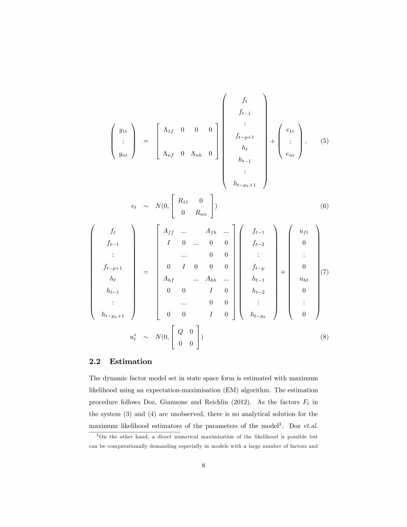
0BBB@y1t

:

ynt

1CCCA =

26664�1f 0 0 0

�nf 0 �nh 0

37775

0BBBBBBBBBBBBBBBBBB@

ft

ft�1

:

ft�p+1

ht

ht�1

:

ht�ph+1

1CCCCCCCCCCCCCCCCCCA

+

0BBB@e1t

:

ent

1CCCA ; (5)

et � N(0;

24 R11 0

0 Rnn

35) (6)

0BBBBBBBBBBBBBBBBBB@

ft

ft�1

:

ft�p+1

ht

ht�1

:

ht�ph+1

1CCCCCCCCCCCCCCCCCCA

=

26666666666666666664

Aff ::: Afh :::

I 0 ::: 0 0

::: 0 0

0 I 0 0 0

Ahf ::: Ahh :::

0 0 I 0

::: 0 0

0 0 I 0

37777777777777777775

0BBBBBBBBBBBBBBBBBB@

ft�1

ft�2

:

ft�p

ht�1

ht�2

:

ht�ph

1CCCCCCCCCCCCCCCCCCA

+

0BBBBBBBBBBBBBBBBBB@

uft

0

:

0

uht

0

:

0

1CCCCCCCCCCCCCCCCCCA

(7)

u�t � N(0;

24 Q 0

0 0

35) (8)

2.2 Estimation

The dynamic factor model set in state space form is estimated with maximum

likelihood using an expectation-maximisation (EM) algorithm. The estimation

procedure follows Doz, Giannone and Reichlin (2012). As the factors Ft in

the system (3) and (4) are unobserved, there is no analytical solution for the

maximum likelihood estimators of the parameters of the model3 . Doz et.al.3On the other hand, a direct numerical maximisation of the likelihood is possible but

can be computationally demanding especially in models with a large number of factors and

8

(2012) show that an alternative and feasible approach in large datasets is to use

the EM algorithm. They also show that the maximum likelihood estimators of

the model�s parameters are consistent estimators of the true parameters even

if the idiosyncratic components are mildly correlated and therefore violate the

normality and diagonal covariance matrix assumption in equation 6. In a large

cross-section, the misspeci�cation error will go to zero and this result will hold

without any constraint on the relative size of the cross-section n and sample

size T .

The EM algorithm is an iterative estimation procedure. More speci�cally,

let bF (k) and b�(k) = n c��(k); bA(k); cQ�(k); bR(k) obe the estimate of the factors and the parameters obtained in the kth iteration.

Then, at the (k + 1)th iteration, (1) in the E-step ("expectation-step") the al-

gorithm uses the Kalman smoother to estimate the common factors bF (k+1)

given b�(k); (2) in the M-step (maximisation-step") an estimate of b�(k+1) givenbF (k+1) is obtained by maximising the expected likelihood. This is achieved

through substitution of the su¢ cient statistics with their expectations, through

a set of multivariate regressions where the unobserved factors are replaced with

their expected values, bFt(k+1) = Eb�(k) (Ftj y1:::yT ) and corrected for estima-tion uncertainty in the common factors. (3) This procedure is repeated until

convergence to a local maximum of the expected likelihood.

As shown in the appendix, an advantage of this state-space approach is the

possibility of recursively obtaining forecasts conditional on assumptions regard-

ing the future evolution of endogenous variables and also of dealing with missing

observations at the beginning of the sample. The state-space approach can also

be applied in the context of BVARs, as done for example in Banbura, Giannone

complex block structure. As an example of an application in nowcasting GDP in Belgium, see

de Antonio Liedo (2015), where the empirical application is executed using the EM algorithm.

Numerical optimisation, the EM algorithm or a combination of the two are used to estimate

dynamic factor models in the nowcasting plugin distributed as part of the software JDemetra+

developed by the National Bank of Belgium (see www.nnb.be/jdemetra).

9

and Lenza (2015).

The unbalanced end-of-sample structure is a natural outcome of our condi-

tional forecasting exercise and the fact that missing values occur at the beginning

of the sample for some of the series that do not have a long history. Technically,

the missing observations are replaced by e¢ cient estimates conditional on the

model parameters and the realisation of all the series over the whole estimation

sample. The idea is used during the estimation process, and is also part of the

procedure that generates the conditional forecasts. All details regarding the use

of the Kalman �lter/smoother in the presence of missing observations can be

found in Durbin and Koopman (2001)4 .

3 Empirical Results

The empirical exercise is focused on the estimation of a forecasting model for

the "Dwellings" residential property price index, which is a weighted average of

re-sale prices for di¤erent types of residential property and geographically covers

all three Regions in Belgium (Brussels, Wallonia and Flanders). All property

price indices are used in real terms: nominal indices are de�ated by the private

consumption de�ator (PCD) for Belgium5 . The dataset and transformations,

the model speci�cation and evaluation of the out-of-sample forecasting ability

of the model are described in detail in the following sub-sections.

4Durbin and Koopman (2001) apply the Kalman �lter to a modi�ed state-space represen-

tation, with yt;�� and R , replaced by yt;�

�and R respectively. The latter are derived from

the former by removing the rows (and, for R the columns too) that correspond to the missing

observations in yobst .5The results are robust to whether the property price indices are taken in nominal or in

real terms. On the other hand, a model in real terms requires us to select a de�ating variable,

which can be arbitrary. We follow the literature and use the PCD (private consumption

de�ator) here. This de�ator is preferred in the literature because it is in general less volatile

than the HICP for example and will therefore dominate the dynamics of the real variables to

a lesser extent.

10

3.1 Data

The quarterly dataset is composed of seven residential property price indices,

and 28 variables describing the Belgian and the euro area economy, including

demand variables (GDP, consumption, investment, exports, imports, residen-

tial investment), price variables (HICP, NCPI and national account de�ators),

unemployment rates, interest rates (a policy rate, a long yield and a mortgage

interest rate for Belgium as well as the two-, �ve- and ten-year German zero-

coupon bond yields) and mortgage loans. The data span the period 1970q1 to

2012q4, except for all the residential property price series which start in 1973q3

and mortgage loans which start in 1980q1. The full list of the variables and

their transformations is given in Table 1.

The property price indices included in the dataset are indices constructed

by the National Bank of Belgium based on the latest releases of data on the

average price and number of transactions published by the FPS Economy. The

data are published with a time lag of two quarters relative to the current quar-

ter. The average price is computed as the average over all re-sale residential

property transactions for which registration fees were paid, as reported to the

Land Registry ("Cadastre, SPF Finances").

The NBB indices are weighted average prices per area and type of housing,

where the weights are the number of transactions. The growth rate of the index

is in�uenced by a change in the average prices of the components rather than

a relative change in the number of transactions. The indices included in the

dataset are the aggregate "Dwellings Country" Index, and the disaggregated

indices, ("Houses Country", "Flats Country ", "Villas Country", "Houses Brus-

sels", "Houses Flanders" and "Houses Wallonia") re�ecting the price trends for

di¤erent types of housing across the Regions. Note that these re-sale property

price indices are not constructed using a repeat sales methodology so they do

not keep track of any improvement in the quality of the house, as is the case with

the S&P/Case-Shiller U.S. National Home Price Index for example. This means

that an increase in the price over time could always re�ect an improvement in

11

house quality rather than an overvaluation.

The longest available property price series starts in 1973q3. A long history

is essential to model accurately the co-movement between residential property

price growth, interest rates and the business cycle, especially in Belgium where

residential property prices (in real terms) exhibited negative growth rates only in

the late 1970s. Since then, the residential property price index has been growing

steadily, rising faster over the period 1986 � 2007 and decelerating since 2008.

During the same period, the Belgian economy went through several recessions

and expansions.

Mortgage loan data are available back to 1980q1. They are computed as the

total mortgage amount divided by the number of loans requested. The data

are published by the Union Professionelle du Crédit (Professional Bankers As-

sociation) and are available on a monthly basis, also during the current forecast

quarter.

The interest rates include a policy rate and a range of interest rates capturing

the yield curve in Belgium and the euro area, and a mortgage interest rate

capturing the interest margin on adjustable-rate mortgages. The policy rate

is the Euribor for the years after the introduction of the euro in 1999 and is

constructed as a weighted average of country rates for the years before.

The o¢ cial MIR mortgage interest rate for Belgium is available back to

2003q1: It is a synthetic rate computed as the weighted average of mortgage

interest rates (MIR) rates up to one year, between one and �ve years and above

ten years initial rate �xation, where the weights are the amounts originated

with the corresponding rate ("new business"). To construct a longer mortgage

interest rate series, the RIR ("retail interest rate") was used for the period

covering 1992q1-2002q4 and an in-house mortgage interest rate was used for the

period 1970q1-1991q4. The long-term bond yield for Belgium is constructed

as the average yield on the secondary (foreign and domestic) market for the

period 1970q1-1991q4. After 1992q1, the long-term bond yield for Belgium

is the 10-year "OLO" rate. For the euro area, the data includes the euro area

synthetic long interest rate, and the two-, �ve- and ten-year zero-coupon German

12

government bond yield.

3.2 Model speci�cation

The dynamic factor model is estimated for the dataset. Five factors (r = 4; rh =

1, see equations 3-4) are included in the factor model. Four of the factors span all

the variables for Belgium and the euro area, as well as the residential property

prices. One factor is "housing-speci�c" and spans only residential property

prices, residential investment and mortgage loans. Three lags (p = 3; ph = 3)

are included in the VAR of the factors. The choice of the number of factors and

the number of lags is based on a comparison of the out-of-sample forecasting

performance of the alternative speci�cations6 .

A dynamic factor with one single factor would imply that all the variables,

real macroeconomic, in�ation, house prices in Belgium and the euro area co-

move perfectly, their dynamics being perfectly synchronised with that of "the

business cycle factor". Intuitively, this is not a realistic representation of the

dataset, given its heterogeneity. Including more factors helps to capture the

common dynamics of interest rates and in�ation apart from the macroeconomic

real variables, while the housing-speci�c factor helps with capturing the fact

that house prices in Belgium have only slowed down once after the beginning of

the 1980s, exhibiting a di¤erent pattern in the dynamics compared to that of

other real variables. Finally, including more factors in the speci�cation may help

improve the in-sample �t of such variables as unemployment, but the improve-

ment in terms of out-of-sample forecasting for the residential property price is

minimal.6These are not shown here but are available upon request.

13

3.3 Forecasting

3.3.1 Model Validation - Recursive Out-of-Sample Unconditional

and Conditional Forecasts

Given the speci�cation described in the previous section, we estimate the dy-

namic factor model and evaluate its forecasting ability in terms of out-of-sample

unconditional and conditional forecasts over an evaluation period. We use an it-

erative procedure to obtain the h-step (h = 1; 4; 8 quarters) ahead out-of-sample

forecasts.

The intuition behind the forecasting approach is the following. Since the

dynamics of all the variables in the model, macroeconomic and house prices, are

driven by the same common factors, information over the forecasting horizon for

the paths of some of the variables in the dataset can be exploited to deduce the

path of the factors over the forecasting horizon. Thus, the methodology works

out the most likely evolution of the factors given the available information over

the forecasting horizon for the conditioning variables. Once the forecast of

the factors has been computed, the forecast of all the variables, the residential

property price index included, can be computed using the previously estimated

parameters. The procedure is illustrated in Figure 1 and is described next.

First, the parameters and the factors are estimated over a given estimation

sample with information on all variables in the dataset. For example, in the

�rst iteration (iter = 1 and t = 1999q4), an initial sample with data on all

the variables spanning the period 1970q1-1999q4 (blue bars in Figure 1) is used

to obtain estimates of � and A and Ft. Then, unconditional and conditional

h-quarter-ahead out-of-sample forecasts are computed. These forecasts are de-

picted with an "x" and a cross "+" on the left- and right-hand panel of Figure

1.

To obtain the unconditional forecast, the same information set as for estima-

tion is used, including all the variables in the dataset up to 1999q4 for the �rst

iteration. No information over the forecasting horizon is used. We call this in-

formation set t. The unconditional forecast is thus computed with information

14

set U � ftg :

To obtain the conditional forecast, information on the paths of �ve con-

ditioning variables (EA policy interest rate, BE OLO 10-year bond yield, BE

PCD, BE GDP and BE mortgage loans de�ated by BE PCD in�ation) over

the forecasting horizon are added to t. We call this information set t+h and

depict it with grey bars in the left-hand panel of Figure 1. The conditional

forecast is thus computed with information set C = ft +t+hg.

The forecast errors are computed as the di¤erence between the actual data

and the forecasts. Then, the sample is increased by one quarter and the process

is repeated over the next iteration (iter = 2 and t = 2000q1). The model is

re-estimated, and h-step-ahead forecasts and the associated forecast errors are

produced. These steps are repeated until all h-step-ahead forecast errors are

computed over the period 2000q1-2012q4.

To summarise, given information U or C and the estimated parametersb� and bA, iterative h-step ahead unconditional or conditional forecasts of thefactors bfUt+h=t , bfCt+h=tand the variables byUt+h=t, byCt+h=t are obtained with theKalman �lter7 . The root mean squared forecast error (root MSFE) is computed

as the average squared error in the evaluation period 8 :

MSFEU;C(h;M) =1

t1 � t0 + 1

t1Xt=t0

1

h

�yobst+h � byU;Ct+h=t (M)

�2(9)

where t1 and t0 denote the start and end of the evaluation period (2000q1 �

2012q4), yobst+h denotes the observation for t + h for the variable, byU;Ct+h=t (M)

denotes the h-step-ahead forecast using model M and the information sets U

or C .

The unconditional forecast of the dynamic factor model is evaluated against

the forecasts obtained from two benchmark models. The �rst is a naive bench-

mark, that is a random walk with drift for the (log -) level of each variable i7More details on the Kalman �lter equations can be found in the Technical Appendix.8The evaluation criterion is univariate as opposed to a multivariate criterion like the log

determinant of the covariance of the forecast errors. This is because the aim here is to evaluate

the speci�c performance of each type of model for property prices and not the overall forecast

performance of the model.

15

in the dataset. The second benchmark model is a vector autoregression (VAR)

which includes six variables: EA policy interest rate, BE OLO 10-year bond

yield, BE PCD, BE GDP, BE residential investment and real residential prop-

erty price index (Dwellings). The variables are transformed in the same way as

for the DFM, so they are taken in log di¤erences. This type of VAR is often used

to obtain empirical estimates of the reaction of house prices to monetary policy,

credit or technology shocks and of the reaction of GDP to shocks to the supply

or demand of housing services (in the framework of dynamic stochastic general

equilibrium models, see for example Iacoviello and Neri (2010), Jarosinksi and

Smets (2008)). Empirical unrestricted VARs allow for more �exibility than tra-

ditional vector error-correction models (VECMs)9 , which link the log level of

house prices to a set of short- and long-run determinants making use of eco-

nomic theory to determine a long-run equilibrium between demand and supply.

If these restrictions do not hold in practice, the forecast obtained from the VAR

will be more accurate.

The DFM forecasts are compared to those obtained with the random walk

and the VAR which uses data available at the time of the forecast. In other words

the same iterative procedure and the information set used for the unconditional

DFM forecast is used for the alternative benchmark model forecasts as well.

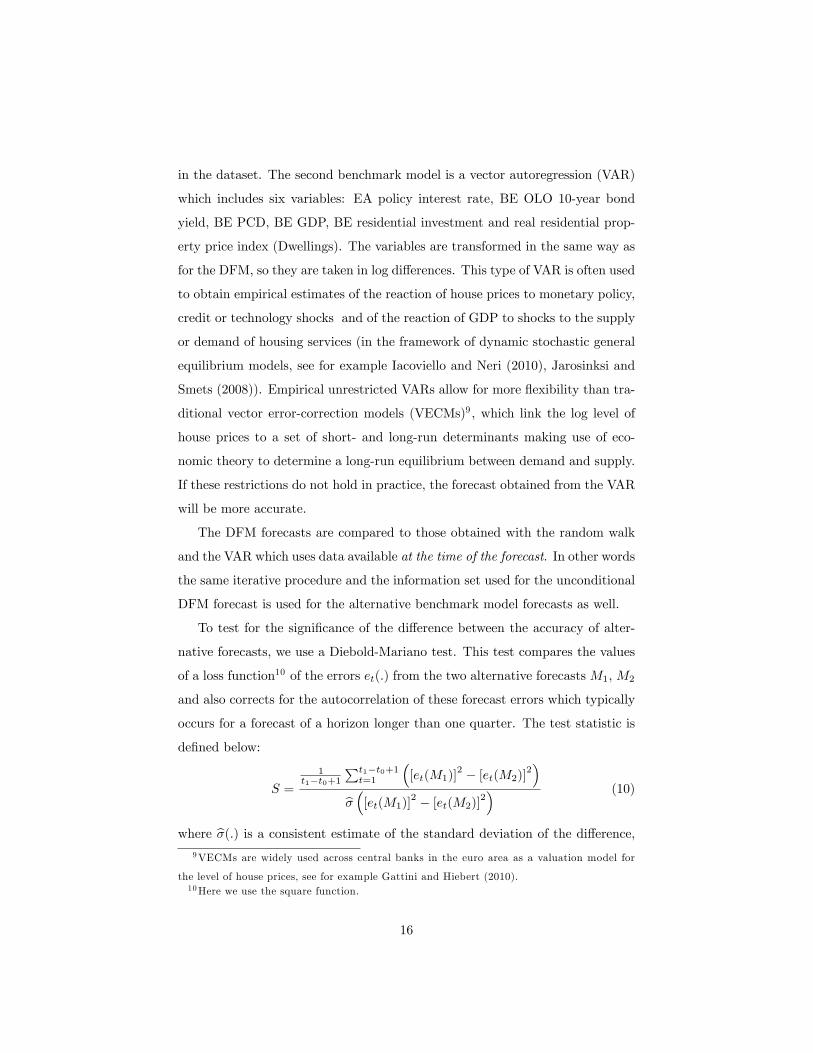
To test for the signi�cance of the di¤erence between the accuracy of alter-

native forecasts, we use a Diebold-Mariano test. This test compares the values

of a loss function10 of the errors et(:) from the two alternative forecasts M1, M2

and also corrects for the autocorrelation of these forecast errors which typically

occurs for a forecast of a horizon longer than one quarter. The test statistic is

de�ned below:

S =

1t1�t0+1

Pt1�t0+1t=1

�[et(M1)]

2 � [et(M2)]2�

b� �[et(M1)]2 � [et(M2)]

2� (10)

where b�(:) is a consistent estimate of the standard deviation of the di¤erence,9VECMs are widely used across central banks in the euro area as a valuation model for

the level of house prices, see for example Gattini and Hiebert (2010).10Here we use the square function.

16

based on the autocovariance generating function with a truncation lag given by

h � 1. Under the null hypothesis of equal forecast accuracy of the two models

the test statistic follows a standard normal distribution.

Table 2 and Table 3 present the results for the unconditional and conditional

forecasts over horizons h = 1; 4; 8 quarters. Table 2 reports the RMSFE ratio of

the DFM and the VAR with respect to a random walk with drift, while Table 3

reports the RMSE ratio of the conditional against the unconditional forecast for

the DFM. In both exercises, the evaluation sample is 2000q1-2012q4. The out-

of-sample 1-quarter and 4-quarters-ahead forecasts and the data are depicted in

Figures 3 to 10.

(Insert Table 2 and Table 3 here)

Table 2 shows that, for h = 1; the DFM forecast for the residential property

price (Dwellings index) outperforms the random walk and the VAR forecast.

However, for h = 4; the unconditional forecast of the VAR outperforms that of

the DFM.

Most of the remaining property price indices are better forecast with the

DFM and the VAR than the random walk over short and longer horizons11 .

At longer horizons, the di¤erence between the two models�performance is not

signi�cant.

In the case of real variables and in�ation, the 1-quarter-ahead unconditional

forecasts of the DFM perform better than the random walk in Belgium and the

euro area. The di¤erence in performance with the random walk disappears for

the 4- and 8-quarter horizon unconditional forecasts. The DFM and the VAR

perform in a similar way. One exception is residential investment, where the

VAR performs slightly better than the DFM.

The results in Table 3 show that conditioning on available information

improves the out-of-sample DFM forecast for the residential property price

(Dwellings) index , especially in the 4-quarter and 8-quarter horizon. The re-

duction in the RMSE of the conditional forecast compared to the unconditional

11The only exception is the Villas index. This is probably due to the idiosyncratic behaviour

of the series.

17

forecast is statistically signi�cant and amounts to 16% (h = 4) and 19% (h = 8).

As expected, most conditional forecasts for the other variables largely im-

prove over the unconditional forecasts. The �ve conditioning variables broadly

capture the evolution of the macroeconomic environment and the reduction in

the RMSE, both at short and long horizons, is large and statistically signi�cant

(see Table 3 ).

3.4 Accounting for Revisions in the Residential Property

Price Forecast in Terms of Changes in the Condition-

ing Assumptions

Next, we illustrate how conditional forecasting can be used to produce forecasts

for house prices which are consistent with given assumptions on the paths of

variables describing the macroeconomic environment in Belgium and the euro

area over a speci�c forecasting horizon. To make the exercise consistent with

the conditioning approach presented in the previous section, the conditioning

variables are those used previously, i.e. EA policy interest rate, BE OLO 10-

year bond yield, BE PCD, BE GDP and BE mortgage loans de�ated by BE

PCD in�ation.

In our example, we focus on the period 2007-2009. In particular, we compute

two conditional forecasts for the "Dwellings" residential property price index

(in real terms) over the period 2007q1-2009q4. For the �rst forecast, which

we assume is performed in September 2007, we show how the model reads the

data and the conditioning information available at that time (left-hand panel

of Figure 2). For the second forecast, which we assume takes place one year

later in September 2008, we show how the house price forecast is revised given

the new data and assumptions available (right-hand panel of Figure 2). We use

expectations on future paths of the conditioning variables as published in the

December 2007 and December 2008 NBB Economic Reviews for each forecast

respectively12 .12The timing of the two forecasts closely resembles that of the Autumn "projection exercise".

18

For the September 2007 forecast, the available residential property price

data only goes up to 2006q4, since the o¢ cial residential property price data

are published with a two-quarter time lag. Thus, the house price forecast will

start in 2007q1 and will use the available data (blue and gray bars in the left-

hand panel of Figure 2) and expectations on the future paths of the conditioning

variables (light grey bars in the left-hand panel of Figure 2).

The second forecast is assumed to be performed in September 2008. Now, the

conditioning information will change as four more quarters of residential prop-

erty price data, covering 2007q1-2007q4 (depicted by a green bar in right-hand

panel of Figure 2) and four more quarters of mortgage loans, GDP, interest rates

and in�ation data, covering the period 2007q4-2008q3 will have been published.

Note that interest rates and mortgage loan data over 2007q1-2007q3 are �nal

(in grey in the right-hand panel of Figure 2) while BE GDP and in�ation over

the same period have been revised (in darker green in right-hand panel of Figure

2). Finally, a new Autumn 2008 scenario over the period 2008q4-2009q413 is

available (in lighter green in right-hand panel of Figure 2).

3.4.1 House prices up to 2007 and a summary of the 2007 and 2008

scenarios

Next we brie�y describe the trends inhouse prices up to 2007 and the December

2007 and December 2008 NBB Economic Review paths for the conditioning

variables.

The year 2006 marked the end of a �ve-year period of upward-trending

residential property price year-on-year growth rates which started in 2000, both

in nominal and real terms. In quarterly growth rate terms, this translated into

an average of 1.7% per quarter growth rate between 2001 and 2006. Growth

rates had already started slowing down during the course of 2006: the average

Therefore expectations for the paths of the conditioning variables, which are published in

December, are already available to the forecaster in September.13Even though the scenarios span over 3 years, only the years relevant to the present fore-

casting exercise are shown.

19

quarterly growth rate in 2006 was equal to 1.85%, lower than the quarterly

growth rate average of 2.38% for 2005. Mortgage loans followed the same trend

(0.15% average growth rate in 2006 against 2.55% in 2005).

The macroeconomic context at the end of 2007, as described in the December

2007 NBB Economic Review, was coloured by the beginning of the �nancial

crisis, with the economy holding up well for the �rst half of 2007 and expected

to remain stable for the remaining part of 2007 and in 2008 (0.5% GDP growth

rate in 2008q4), even though the uncertainty surrounding these projections was

high. GDP growth was expected to be sustained by internal consumption growth

and investment. Exports were not expected to be a¤ected much by the �nancial

developments abroad, as it was thought that the crisis, mainly in the US at

that time, would be contained in the �nancial sector and would not spill over

to the real economy. On the price front, rising oil prices and the appreciation

of the euro were driving an acceleration of both euro area and Belgian in�ation.

The policy rate and Belgian 10-year bond yields were expected to decline very

slightly.

The picture had changed by the end of 2008. Even though the situation had

been stable up to mid-2008, soon after that it became clear that the �nancial

crisis had spilled over to the real economy, drastically curtailing international

demand and inducing a decrease in oil prices. As a result, GDP growth for

Belgium was revised downwards in the December 2008 NBB Economic Review,

when it was forecast to slow down signi�cantly for 2008 and drop in 2009, while

in�ation, having reached a peak in mid-2008, was projected to drop in 2009. In

this context, policy interest rates were cut in 2008 and were forecast to be even

lower in 2009, while long-term rates rose slightly as a result of pressure from

deteriorating public �nances.

20

3.4.2 The residential property price forecast and the impact of the

change in the macroeconomic environment

How were the paths of the conditioning variables (December 2007 NBB Eco-

nomic Review) taken into account by the model to produce the Autumn 2007

house price forecast? And then, one year later, what was the impact of the

negative evolution of the macroeconomic environment (December 2008 NBB

Economic Review) on the residential property price forecast when the Autumn

2008 forecast was produced? Table 4 and Figure 11 show the results.

(Insert Table 4 and Figure 11 here)

Table 4 reports the conditional forecast for the residential property price

index (Dwellings) between 2007q1 and 2009q4.

Accuracy of the Autumn 2007 forecast for 2007q1-2007q4 The average

of Autumn 2007 forecast of the quarterly growth rates of the Dwellings index in

2007q1-2007q4 equals 0.5%. This average is substantially lower than the actual

average growth rate computed a year later with the �nal data for the Dwellings

index for 2007q1-2007q4 and the Autumn 2008 PCD in�ation data (line 3 in the

table). This average equals 1.8% 14 . The Autumn 2007 forecast is computed

conditionally on data from mortgage loans and the macroeconomic environment.

The forecast error shows that these "fundamental" factors were not su¢ cient to

capture house prices during 2007. However, the forecast error for the period is

not higher than the RMSE computed for the forecast evaluation exercise in the

previous section.

Accuracy of the Autumn 2007 forecast for 2008q1-2008q4 and 2009q1-

2009q4 The average of Autumn 2007 forecasts for the quarterly growth rates

of the Dwellings index in 2008q1-2008q4 and 2009q1-2009q4 equals 0.3% and

0.4% respectively. These lie below the unconditional forecast for house prices

mainly because, as we saw earlier, the outlook for GDP growth in the Autumn

14When the �nal data for PCD is released the average quarterly growth rate for the Dwellings

index will be lower, at 1.1%.

21

2007 projection exercise had already deteriorated at the onset of the �nancial

crisis. The role of interest rates and in�ation is only minor at this point in time.

Accuracy of the Autumn 2008 forecast for 2008q1-2008q4 and 2009q1-

2009q4 In 2008q3, when the Autumn 2008 forecast is made, the latest avail-

able data for house prices ends in 2007q4. Thus, the Autumn 2008 forecast

starts in 2008q1. The Autumn 2008 forecast for the Dwellings index in 2008

and 2009 equals 0.2% and -0.4% respectively15 , while the data de�ated by the

�nal data on BE PCD in�ation in 2008 and 2009 equals 0.3% and 0.5% 16 . On

average, the forecast error in 2008 is very small while, in 2009, it is close to the

RMSFE computed for the forecast evaluation exercise in the previous section.

Explaining the Autumn 2008 forecast for 2008q1-2008q4 and 2009q1-

2009q4 What is the reason behind the downward revision of the quarterly

growth rate of house prices in 2008 and 2009? The second part of Table 4 shows

us how current and past forecast errors in the conditioning variables contribute

to the forecast update of the residential property price17 .

In 2008q1 for example, the new forecast is 0.27% higher than the previous

one. This is mainly due to negative growth in lending in 2008q1 and past positive

innovations in house prices still having informative content even if there are no

current house price data available18 .

The slightly positive component for BE GDP (0.14%) comes from the current

and past quarters�positive components. The same pro�le holds for 2008q2 and

15As previously, forecasts and data in the text are computed as averages of quarterly growth

rates within the year, as shown in Table 4.16The same averages for house prices de�ated by the Autumn 2008 PCD scenario are slightly

higher, 0.8% and 0.7% in 2008 and 2009 respectively.17See the Technical Appendix for the details on how this decomposition is obtained as a

by-product of the Kalman �lter iterations.18The relative importance of past house prices in the current forecast can be seen more

clearly in Figure 13 were the impact coe¢ cients ij are displayed : i is the BE residential

property price index (Dwellings) and j are the �ve macroeconomic conditioning variables.

More details on impact coe¢ cients can be found in the Technical Appendix.

22

2008q3, except that now the information derived from mortgage loans is close

to 0% for 2008q2 and negative for 2008q3 (-0.48%). The information on past

house price data is discounted more heavily as it becomes older and therefore

plays a decreasing role.

Starting from 2008q4, the same forces are at play but to a smaller extent as

now there is no new information from mortgage loans.

In 2008q4, GDP plays as big a role as past mortgage loans and past house

prices in explaining the -0.46% downward revision in the Autumn 2007 house

price forecast. Added to this is information from short- and long-term interest

rates in 2009q1 and 2009q2 which plays a more important role19 .

Finally, in 2009q4, a higher spread caused by higher long-term interest rates

and lower short-term interest rates implies an overall decline in the residential

property price index of �0:13%20 . Additionally, the lower-than-expected GDP

growth rate and higher-than-expected in�ation rate imply a further drop in the

residential property price index by �0:27% and �0:02% respectively. Overall,

the impact of the revised paths of the macroeconomic conditioning variables on

the residential property price forecast is equal to �0:63% for 2009q4:

4 Conclusion

The paper has forecast the residential property price index in Belgium with a

dynamic factor model estimated with maximum likelihood and the EM algo-

rithm.

The dynamic factor model has been estimated with a dataset of macroeco-

nomic variables describing the Belgian and euro area economy. The model has

19Figure 13 depicts the impact coe¢ cients for the forecast in 2009q1. Note that in the

absence of current information from mortgage loans, the current impact coe¢ cient ( � = 0) is

zero. The importance of GDP is higher with respect to the situation in 2008q1 when mortgage

loan data together with very recent house price data were available. The impact coe¢ cients

of the short and long interest rates are unchanged and in�ation plays virtually no role.20 -0.13% is obtained as the sum of -0.26% update related to the BE Long IR and 0.13%

update related to the Short IR.

23

been validated with recursive unconditional out-of-sample forecasts against a

random walk with drift and a vector autoregressive benchmark. Conditional

out-of-sample forecasts have been obtained recursively over the period 2000q1-

20012q4 and have been shown to improve over unconditional forecasts. A fore-

casting exercise has illustrated how information from mortgage loans, interest

rates, GDP and in�ation is combined in forecasting residential property prices

in Belgium.

The forecast for property prices over 2008q1-2009q4 was relatively accu-

rate during 2008 while it clearly underestimated quarterly growth rates in 2009.

Given the model�s impact coe¢ cients, lower quarterly growth rates were ex-

pected as a result of the spillover of the �nancial crisis to the real economy.

This deceleration materialised only in part, during 2008. By the end of 2009,

house prices were accelerating again.

There are two limitations to the approach used for this paper. The �rst is

that, at this stage, it is a reduced-form exercise. Future work may focus on

identi�cation of the shocks and their impact on the residential property price

index forecast. The second limitation is that this approach does not deliver an

equilibrium level for the real residential property price index. As a result, this

type of model is not suited for identifying periods of price misalignments and

bubbles in the property market.

However, the forecasting approach, based on the Kalman �lter modi�ed for

ragged-edge data structures, is �exible, easily adaptable to a larger dataset or to

data with di¤erent frequencies and can be used to produce real-time forecasts as

well as other types of scenario analysis, such as risk analysis and stress-testing.

24

ReferencesAntonio Liedo David (2015). Nowcasting Belgium, Eurostat Review of National

Accounts and Macroeconomic Indicators, 2, 7-41.

Bai J. and S. Ng (2002). Determining the Number of Factors in Approximate

Factor Models. Econometrica, 70(1), pages 191-221.

Banbura M., D. Giannone and M. Lenza (2015). Conditional Forecasts and

Scenario Analysis with Vector Autoregressions for Large Cross-Sections, Inter-

national Journal of Forecasting, forthcoming.

Banbura M., Domenico Giannone and Lucrezia Reichlin (2010). Nowcasting,

in Michael P. Clements and David F. Hendry, editors, Oxford Handbook on

Economic Forecasting, forthcoming

Banbura M. and M. Modugno(2014). Maximum likelihood estimation of factor

models on datasets with arbitrary pattern of missing data, Journal of Applied

Econometrics, 29, pages 133-160

Banbura M. and Gerhard Rünstler (2011). A look into the factor model black

box: Publication lags and the role of hard and soft data in forecasting GDP,

International Journal of Forecasting, Elsevier, vol. 27(2), pages 333-346.

Boivin, J. and S. Ng (2003). Are more data always better for factor analysis?,

Journal of Econometrics 127, pages 169-94.

Case B. and Susan Wachter (2005). Residential real estate price indices as

�nancial soundness indicators: methodological issues, BIS Papers n.21, April

2005, Bank of International Settlements

Claessens S. , M. Ayhan Cose and Marco E. Terrones (2008). What Happens

During Recessions, Crunches and Busts?, Working Paper, WP/08/274, Inter-

national Monetary Fund .

Doz Catherine, Domenico Giannone, and Lucrezia Reichlin (2012). A quasi-

maximum likelihood approach for large approximate dynamic factor models,

Review of Economics and Statistics, Review of Economics and Statistics vol.

94(4), pages 1014-1024.

Doz Catherine, Domenico Giannone, and Lucrezia Reichlin (2011). A two-

step estimator for large approximate dynamic factor models based on Kalman

25

�ltering, Journal of Econometrics, vol. 164(1), pages 188-205.

Durbin J. and Koopman S. J. (2001). Time series analysis by state-space meth-

ods. Oxford University Press.

Eickmeier, Sandra and Hofmann, Boris (2013). Monetary Policy, Housing

Booms, And Financial (Im)Balances, Macroeconomic Dynamics, Cambridge

University Press, vol. 17(04), pages 830-860, June.

Forni, M. M. Hallin, M. Lippi and L. Reichlin (2000). The Generalized Dy-

namic Factor Model: Identi�cation and Estimation, Review of Economics and

Statistics, 82, pages 570-554.

Forni, M. M. Hallin, M. Lippi and L. Reichlin (2004). The Generalized Dynamic

Factor Model: Consistency and Rates. Journal of Econometrics, 119, pages 231-

245.

Forni Mario, Domenico Giannone, Marco Lippi, and Lucrezia Reichlin (2009)

Opening the black box: Structural factor models with large cross-sections,

Econometric Theory, Vol. 25, No. 05, pages 1319-1347.

Gattini, Luca & Hiebert, Paul, 2010. "Forecasting and assessing Euro area

house prices through the lens of key fundamentals," Working Paper Series 1249,

European Central Bank.

Giannone, D., Lenza, M., and Reichlin, L. (2010). Business cycles in the euro

area. In A. Alesina & F. Giavazzi (Eds.), Europe and the Euro (pp. 141�167).

National Bureau of Economic Research, Inc.

Girouard N., Mike Kennedy, Paul van den Noord, Christophe André (2006),

�Recent House Price Developments: The Role of Fundamentals�, OECD Eco-

nomics Department Working Papers, No. 475, OECD

Heathcote J. and Morris Davis (2005). Housing and the Business Cycle, Inter-

national Economic Review August 2005, 46/3, pages 751-784.

Iacoviello, Matteo and Stefano Neri. (2010). "Housing Market Spillovers:

Evidence from an Estimated DSGE Model." American Economic Journal:

Macroeconomics, 2(2): 125-64.

Jarocinski M. and Frank Smets (2008). House Prices and the Stance of Monetary

Policy, Federal Reserve Bank of St. Louis Review, July/August 2008, 90(4), pp.

26

339-65.

Leamer E. (2007). Housing IS the Business Cycle, NBER Working Paper No.

13428

Luciani M. (2013). Monetary policy and the housing market: A structural factor

analysis, Journal of applied econometrics, 2013, doi: 10.1002/jae.2318

Poterba, J. (1984), �Tax Subsidies to Owner-Occupied Housing: An Asset Mar-

ket Approach�, Quarterly

Journal of Economics, 99, 729-752.

Quah D. and T. J. Sargent (1993), a Dynamic Index Model for Large Cross-

Sections in Business cycles, Indicators and Forecasting, NBER, pages 285-310

Stock J. and Mark Watson (2002). Macroeconomic Forecasting Using Di¤usion

Indexes, Journal of Business Economics Statistics, 20, pages 147-162

Stock J. and Mark Watson (2003). Forecasting Output and In�ation: The Role

of Asset Prices, Journal of Economic Literature Vol.XLI September 2003, pages

788-829.

Stock J. and Mark Watson (2011). Dynamic Factor Models, in The Oxford

Handbook of Economic Forecasting ed. by M.P. Clements, and D. F. Hendry.

Oxford University Press.

Stock, J. and Mark Watson, (2012). Disentangling the channels of the 2007�

2009 recession, NBER Working Papers 18094. National Bureau of Economic

Research, Inc.

27

AppendixTechnical Appendix

We provide a short description of the Kalman �lter iterations used for forecasting

conditional on information from a subset of the variables byobst in the dataset.

The �lter gain and innovations are used to compute the forecast update and its

decomposition.

Formally, we are interested in obtaining the forecast of the residential property

price index for Belgium, yit, at time t > t0, conditional on the available time

series for a subset of the data. The conditional forecast uses information from

data or future scenarios for a subset of variables in yt,, for t > t0; whenever this

information or scenario is available21 .

As for the unconditional forecast, QMLE estimation over t = 1; ::; t0 yields

estimates of the factors, and the model parameters b�=t0 ;� bA�=t0

; bR=t0 and dQ=t0 .Once these estimates are obtained, the Kalman �lter is applied on the state

space representation of the model in eq. 3 and 4. The �lter is nevertheless

modi�ed to take into account the fact that there is no information for t > t0 for

the variables that are forecast (residential property prices). These variables can

be assimilated to series with "missing observations" and the approach of Durbin

and Koopman (2001) can be used to obtain the forecasts. The �lter is modi�ed

by removing the rows in Yt and the rows and columns in R that correspond to

the series with the missing values. Then, the Kalman �lter iterations are run as

usual to obtain the path of the estimated factors conditional on the variables in

yobst : These variables are observed either because they are available earlier than

the residential property price or because there is a scenario that we would like

to impose.

The conditional mean of the factor Ft based on information available at time

t � 1 is de�ned as Ft=t�1 = E(Ftj yobs1 :::yobst�1) and the conditional variance as

Pt=t�1 = var(Ftjyobs1 :::yobst�1): The Kalman �lter equations compute Ft=t = E(Ftj21The conditional forecast used here is in "reduced-form" in the sense that the scenario is

imposed on the future paths of the variables and not on the future paths of the structural

("identi�ed") shocks.

28

yobs1 :::yobst ) and Pt=t = var(Ftjyobs1 :::yobst ) :

Ft=t = Ft=t�1 +Ktvt (11)

Pt=t = Pt=t�1 �KtPt=t�1b�0(12)

where

vt = yobst � b�Ft=t�1 (13)

Kt = Pt=t�1b�0�b�Pt=t�1b�0

+ bR��1 (14)

The variable vt is the measurement equation innovation or "prediction error"

and the term�b�Pt=t�1b�0

+ bR� is de�ned as the variance of the prediction errorvar(vt). Kt is the Kalman gain matrix.

The prediction equations of the Kalman �lter compute Ft+1=t = E(Ft+1j yobs1 :::yobst )

and Pt+1=t = var(Ft+1jyobs1 :::yobst ) using:

Ft+1=t = bAFt=t (15)

Pt+1=t = APt=tA0+BB

0(16)

Once the path of the factors is known, the conditional forecast byt for any variablein yt (whether the variables is observed or not) is given by:

byt = b�Ft=tBy replacing recursively, we �nd:

byt = �Atf0=0 + �At�1K1v1 + �A

t�2K2v2 + :::

:::+ �AKt�1vt�1 + �Ktvt (17)

TheN elements in �0

i, the row that corresponds to the ith variable in the loadings

matrix � , inform us which factors are important for forecasting yi (eq.17). The

(r;N) elements of the Kalman gain Kt tell us which part of the innovation vt

in each of the N series is used to update the factors Ft, or, in other words

which part of the innovation corresponds to the common shock ut as opposed to

the measurement error/idiosyncratic component et (eq. 3). The last equation

29

(eq. 17) tells us that at each point in time t, we can decompose the conditional

forecast for each variable into a weighted sum of all current and past forecast

errors:

byit =NXj=1

tX�=0

ij(�)vj;t�� (18)

=NXj=1

cij;t (19)

The weights ij(�) depend on the estimated loadings matrix and the Kalman

gain. In this model, the loadings and the Kalman gain are time-invariant. The

Kalman gain nevertheless depends on the pattern of the missing values in the

observed variables (see Banbura and Runstler (2011)). As this pattern changes

at each point in time, so will the weights ij(�).

30

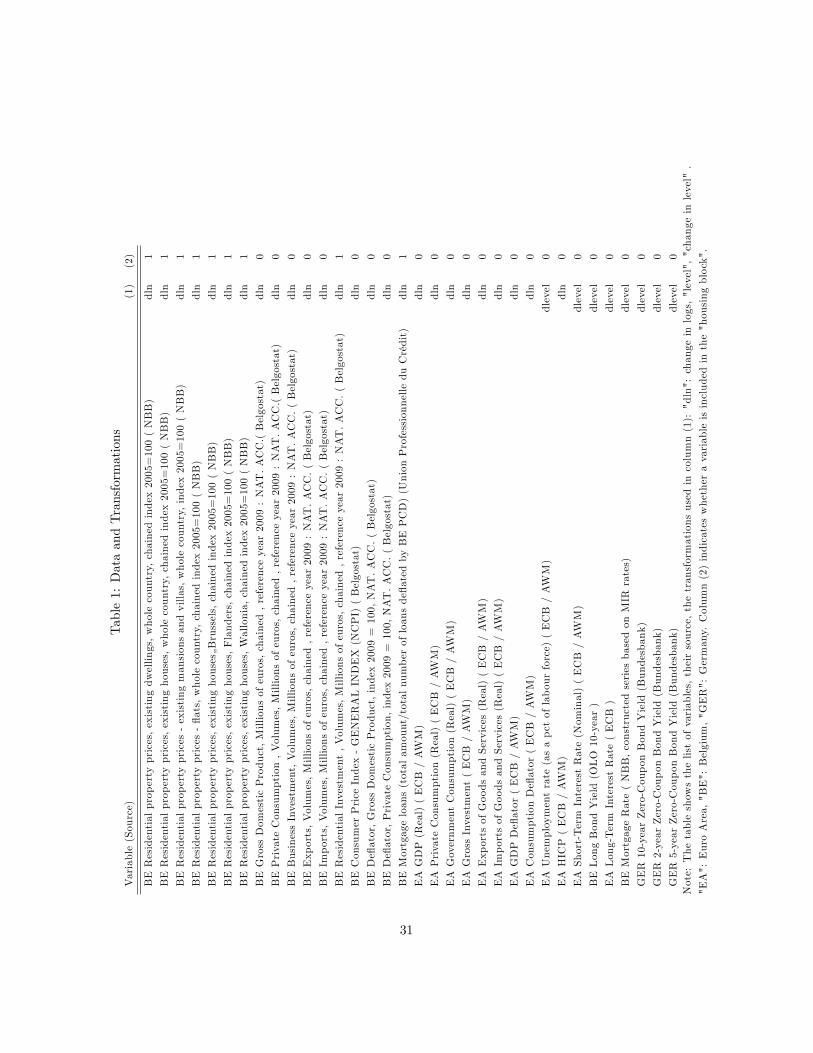
Table1:DataandTransformations

Variable(Source)

(1)

(2)

BEResidentialpropertyprices,existingdwellings,wholecountry,chainedindex2005=100(NBB)

dln

1

BEResidentialpropertyprices,existinghouses,wholecountry,chainedindex2005=100(NBB)

dln

1

BEResidentialpropertyprices-existingmansionsandvillas,wholecountry,index2005=100(NBB)

dln

1

BEResidentialpropertyprices-�ats,wholecountry,chainedindex2005=100(NBB)

dln

1

BEResidentialpropertyprices,existinghouses�Brussels,chainedindex2005=100(NBB)

dln

1

BEResidentialpropertyprices,existinghouses,Flanders,chainedindex2005=100(NBB)

dln

1

BEResidentialpropertyprices,existinghouses,Wallonia,chainedindex2005=100(NBB)

dln

1

BEGrossDomesticProduct,Millionsofeuros,chained,referenceyear2009:NAT.ACC.(Belgostat)

dln

0

BEPrivateConsumption,Volumes,Millionsofeuros,chained,referenceyear2009:NAT.ACC.(Belgostat)

dln

0

BEBusinessInvestment,Volumes,Millionsofeuros,chained,referenceyear2009:NAT.ACC.(Belgostat)

dln

0

BEExports,Volumes,Millionsofeuros,chained,referenceyear2009:NAT.ACC.(Belgostat)

dln

0

BEImports,Volumes,Millionsofeuros,chained,referenceyear2009:NAT.ACC.(Belgostat)

dln

0

BEResidentialInvestment,Volumes,Millionsofeuros,chained,referenceyear2009:NAT.ACC.(Belgostat)

dln

1

BEConsumerPriceIndex-GENERALINDEX(NCPI)(Belgostat)

dln

0

BEDe�ator,GrossDomesticProduct,index2009=100,NAT.ACC.(Belgostat)

dln

0

BEDe�ator,PrivateConsumption,index2009=100,NAT.ACC.(Belgostat)

dln

0

BEMortgageloans(totalamount/totalnumberofloansde�atedbyBEPCD)(UnionProfessionnelleduCrédit)

dln

1

EAGDP(Real)(ECB/AWM)

dln

0

EAPrivateConsumption(Real)(ECB/AWM)

dln

0

EAGovernmentConsumption(Real)(ECB/AWM)

dln

0

EAGrossInvestment(ECB/AWM)

dln

0

EAExportsofGoodsandServices(Real)(ECB/AWM)

dln

0

EAImportsofGoodsandServices(Real)(ECB/AWM)

dln

0

EAGDPDe�ator(ECB/AWM)

dln

0

EAConsumptionDe�ator(ECB/AWM)

dln

0

EAUnemploymentrate(asapctoflabourforce)(ECB/AWM)

dlevel

0

EAHICP(ECB/AWM)

dln

0

EAShort-TermInterestRate(Nominal)(ECB/AWM)

dlevel

0

BELongBondYield(OLO10-year)

dlevel

0

EALong-TermInterestRate(ECB)

dlevel

0

BEMortgageRate(NBB,constructedseriesbasedonMIR

rates)

dlevel

0

GER10-yearZero-CouponBondYield(Bundesbank)

dlevel

0

GER2-yearZero-CouponBondYield(Bundesbank)

dlevel

0

GER5-yearZero-CouponBondYield(Bundesbank)

dlevel

0Note:Thetableshowsthelistofvariables,theirsource,thetransformationsusedincolumn(1):"dln":changeinlogs,"level","changeinlevel".

"EA":EuroArea,"BE":Belgium,"GER":Germany.Column(2)indicateswhetheravariableisincludedinthe"housingblock".

31

Table 2: Ratio of RMSFE for DFM and VAR relative to a random walk withdrift benchmark: Unconditional forecasts

DFM VAR

h=1 h=4 h=8 h=1 h=4 h=8

BE Property Price (Dwellings), real 0.78��� 0.86 0.94 0.83� 0.88� 1.02

BE Prop.P. houses, real 0.78��� 0.88 0.93

BE Prop.P. villas, real 1.02 1.05 1.12

BE Prop.P, �ats, real 0.92� 0.98 1.00

BE Prop. P. houses, Brussels, real 0.96 0.95 0.96

BE Prop. P, houses, Flanders, real 0.84�� 0.88 0.95

BE Prop.P, houses, Wallonia, real 0.86�� 0.98 0.99

BE Real GDP 0.82� 1.01 1.02 0.89 1.00 1.19

BE Private consumption 1.01 1.10 1.09

BE Gross �xed capital formation 0.93� 0.98 0.97

BE Exports 0.92 1.01 0.98

BE Imports 0.90 1.02 0.98

BE Residential Investment 0.98�� 1.03 1.08 0.75� 1.33 2.21

BE NICP 1.08 1.23 1.12

BE Private consumption de�ator 1.23 1.17 1.06 1.34 1.32 1.42

BE GDP de�ator 1.09 1.20 1.16

BE Mortgage loans, real 6.36 6.84 6.70

EA Real GDP 0.82� 1.07 1.06

EA Private Consumption 0.96 1.15 1.19

EA Gov. Consumption 0.98 0.99 1.07

EA Gross Investment 0.87� 1.07 1.04

EA Exports 0.85� 1.03 0.97

EA Imports 0.81�� 1.05 1.03

EA GDP De�ator 0.60��� 0.79��� 0.93

EA Consumption De�ator 0.66��� 1.00 1.02

EA Unemployment rate 0.62��� 0.62�� 0.60

EA HICP 0.81�� 1.05 1.10

EA Short-Term IR 0.73� 0.96 0.93 0.84 1.10 1.05

BE Long-Term IR 1.00 0.97 0.96 1.02 1.15 1.15

EA Long-Term IR 1.05 0.98 0.99

BE Mortgage IR 0.86� 0.92 0.92

GER 10-year ZC Bond Yield 1.00 1.02 0.98

GER 5-year ZC Bond Yield 0.98 1.01 0.96

GER 2-year ZC Bond Yield 0.92 0.98 0.95Note: The table reports the ratio of the root mean squared forecast errors (RMSFE) of the

DFM and the VAR over the RMSFE of a random walk with drift for each variable. The ratio

is reported for unconditional forecasts h=1, 4 and 8 quarters ahead over the period 2000q1-

2012q4. A value smaller than one indicates that the RMSFE of that model is lower than the

RMSFE of the random walk for that variable. An asterisk (*,**,***) denotes that the null of

equal forecast accuracy between the model and the random walk is rejected at the 90, 95, 99

percent level correspondingly (Diebold-Mariano test). The transformations of the variables

can be found in Table 1.

32

Table 3: Ratio of RMSFE for conditional relative to unconditional forecast.h=1 h=4 h=8

BE Property Price (Dwellings), real 0.99 0.84�� 0.81�

BE Prop.P. existing houses, country, real 1.01 0.84�� 0.84�

BE Prop.P. villas, country, real 1.02 0.91� 0.87��

BE Prop.P, �ats, country, real 0.98 0.96 0.89

BE Prop. P. houses, Brussels, real 0.99 0.99 0.98

BE Prop. P, houses, Flanders, real 1.00 0.90� 0.87�

BE Prop.P, houses, Wallonia, real 1.01 0.89�� 0.89�

BE Real GDP 0.69��� 0.56��� 0.51���

BE Private consumption 0.87��� 0.79��� 0.76���

BE Gross �xed capital formation 0.94��� 0.88��� 0.84���

BE Exports 0.87�� 0.79�� 0.77��

BE Imports 0.84�� 0.75�� 0.72��

BE Residential Investment 0.99 0.83��� 0.74���

BE NICP 0.90 0.83��� 0.87��

BE Private consumption de�ator 0.84��� 0.82��� 0.89���

BE GDP de�ator 0.91 0.85��� 0.85��

BE Mortgage loans, real 0.90��� 0.83��� 0.81���

EA Real GDP 0.78��� 0.65��� 0.62���

EA Private Consumption 0.91��� 0.80��� 0.76���

EA Gov. Consumption 1.01 1.01 0.97

EA Gross Investment 0.90�� 0.79�� 0.76��

EA Exports 0.85�� 0.76�� 0.74���

EA Imports 0.87�� 0.72��� 0.67���

EA GDP De�ator 1.01 0.93 0.88

EA Consumption De�ator 0.92 0.79�� 0.79�

EA Unemployment rate 0.95�� 0.96�� 0.94��

EA HICP 0.88 0.79�� 0.74�

EA Short-Term IR 0.91� 0.65� 0.64�

BE Long-Term IR 0.62��� 0.58��� 0.56���

EA Long-Term IR 0.62��� 0.59��� 0.55���

BE Mortgage IR 1.26 1.25 1.20

GER 10-year ZC Bond Yield 0.76��� 0.74��� 0.71���

GER 5-year ZC Bond Yield 0.75��� 0.71��� 0.69���

GER 2-year ZC Bond Yield 0.76�� 0.70�� 0.68��

Note: The table reports the ratio of the root mean squared forecast errors (RMSFE) of the

DFM for a forecast conditional on EA Short interest rate, BE long yield, BE GDP, BE PCD

in�ation and BE mortgage loans de�ated by PCD and an unconditional forecast. The ratio

is reported for forecasts h=1, 4 and 8 quarters ahead over the period 2000q1-2012q4. A

value smaller than one indicates that the RMSFE of the conditional forecast is lower than the

RMSFE of the unconditional forecast for that variable. Asterisks (***, **,*) denote that the

null of equal forecast accuracy is rejected at the 99, 95, and 90 percent level (Diebold-Mariano

test). The transformations of the variables can be found in Table 1.

33

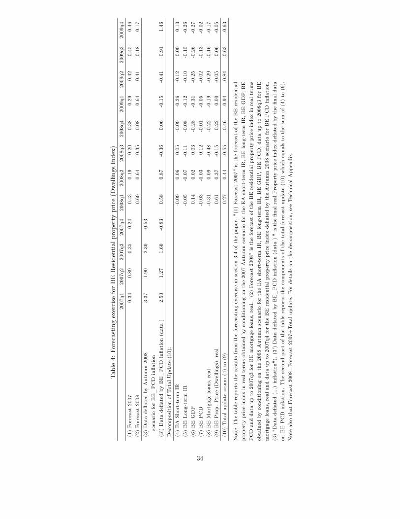
Table4:ForecastingexerciseforBEResidentialpropertyprice(DwellingsIndex)

2007q1

2007q2

2007q3

2007q4

2008q1

2008q2

2008q3

2008q4

2009q1

2009q2

2009q3

2009q4

(1)Forecast2007

0.34

0.89

0.35

0.24

0.43

0.19

0.20

0.38

0.29

0.42

0.45

0.46

(2)Forecast2008

0.69

0.64

-0.35

-0.08

-0.64

-0.41

-0.18

-0.17

(3)Datade�atedbyAutumn2008

3.37

1.90

2.30

-0.53

scenarioforBE_PCDin�ation

(3�)Datade�atedbyBE_PCDin�ation(data)

2.50

1.27

1.60

-0.83

0.58

0.87

-0.36

0.06

-0.15

-0.41

0.91

1.46

DecompositionofTotalUpdate(10):

(4)EAShort-term

IR-0.09

0.06

0.05

-0.09

-0.26

-0.12

0.00

0.13

(5)BELong-term

IR-0.05

-0.07

-0.11

-0.08

-0.12

-0.10

-0.15

-0.26

(6)BEGDP

0.14

0.02

0.03

-0.28

-0.31

-0.25

-0.26

-0.27

(7)BEPCD

-0.03

-0.03

0.12

-0.01

-0.05

-0.02

-0.13

-0.02

(8)BEMortgageloans,real

-0.31

0.09

-0.48

-0.22

-0.19

-0.29

-0.16

-0.17

(9)BEProp.Price(Dwellings),real

0.61

0.37

-0.15

0.22

0.00

-0.05

0.06

-0.05

(10)Totalupdate=sum(4)to(9)

0.27

0.44

-0.55

-0.46

-0.94

-0.84

-0.63

-0.63

Note:Thetablereportstheresultsfrom

theforecastingexerciseinsection3.4ofthepaper."(1)Forecast2007"istheforecastoftheBEresidential

propertypriceindexinrealtermsobtainedbyconditioningonthe2007AutumnscenariofortheEAshort-term

IR,BElong-term

IR,BEGDP,BE

PCDanddataupto2007q3forBEmortgageloans,real."(2)Forecast2008"istheforecastoftheBEresidentialpropertypriceindexinrealterms

obtainedbyconditioningonthe2008AutumnscenariofortheEAshort-term

IR,BElong-term

IR,BEGDP,BEPCD,dataupto2008q3forBE

mortgageloans,realanddataupto2007q4fortheBEresidentialpropertypriceindexde�atedbytheAutumn2008scenarioforBEPCDin�ation.

(3)"Datade�ated(...)in�ation").(3�)Datade�atedbyBE_PCDin�ation(data)"isthe�nalrealPropertypriceindexde�atedbythe�naldata

onBEPCDin�ation.Thesecondpartofthetablereportsthecomponentsofthetotalforecastupdate(10)whichequalstothesumof(4)to(9).

NotealsothatForecast2008=Forecast2007+Totalupdate.Fordetailsonthedecomposition,seeTechnicalAppendix.

34

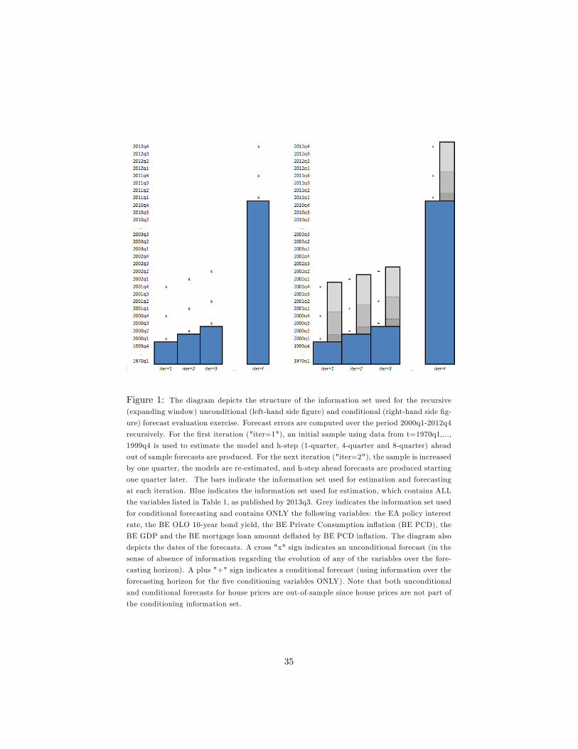
Figure 1: The diagram depicts the structure of the information set used for the recursive

(expanding window) unconditional (left-hand side �gure) and conditional (right-hand side �g-

ure) forecast evaluation exercise. Forecast errors are computed over the period 2000q1-2012q4

recursively. For the �rst iteration ("iter=1"), an initial sample using data from t=1970q1,...,

1999q4 is used to estimate the model and h-step (1-quarter, 4-quarter and 8-quarter) ahead

out of sample forecasts are produced. For the next iteration ("iter=2"), the sample is increased

by one quarter, the models are re-estimated, and h-step ahead forecasts are produced starting

one quarter later. The bars indicate the information set used for estimation and forecasting

at each iteration. Blue indicates the information set used for estimation, which contains ALL

the variables listed in Table 1, as published by 2013q3. Grey indicates the information set used

for conditional forecasting and contains ONLY the following variables: the EA policy interest

rate, the BE OLO 10-year bond yield, the BE Private Consumption in�ation (BE PCD), the

BE GDP and the BE mortgage loan amount de�ated by BE PCD in�ation. The diagram also

depicts the dates of the forecasts. A cross "x" sign indicates an unconditional forecast (in the

sense of absence of information regarding the evolution of any of the variables over the fore-

casting horizon). A plus "+" sign indicates a conditional forecast (using information over the

forecasting horizon for the �ve conditioning variables ONLY). Note that both unconditional

and conditional forecasts for house prices are out-of-sample since house prices are not part of

the conditioning information set.

35

Figure 2: The diagram shows the structure of the conditioning information used to compute

the residential property price forecast in September 2007 (left-hand side) and in September

2008 (right-hand side). The vertical axis depicts the reference period of the conditioning

variables over the forecast horizon which is shown in light red. The horizontal axis is split

in two. The left hand side represents the information for the conditioning variables used in

September 2007. The right-hand side represents the information used in September 2008.

In both cases, the model is estimated with data over 1970q1-2006q4. Up to 2006q4 the

conditioning data set contains �nal data for ALL variables (see Table 1) (dark blue in the

�gure). Darker grey (or green) indicates �nal data as released in 2007q3 (or in 2008q3).

Lighter grey or green indicates a scenario : "Autumn 2007" scenario for the forecasting exercise

in 2007q3 and "Autumn 2008" scenario for the forecasting exercise in 2008q3. The bright red

square highlights when the forecasting exercise for the residential property price is performed.

No information over the forecast horizon is available for any of the house prices in 2007q3.

In 2008q3 the red square is above the dark green bar for the residential property price index

because of a 6-month publication lag.

36

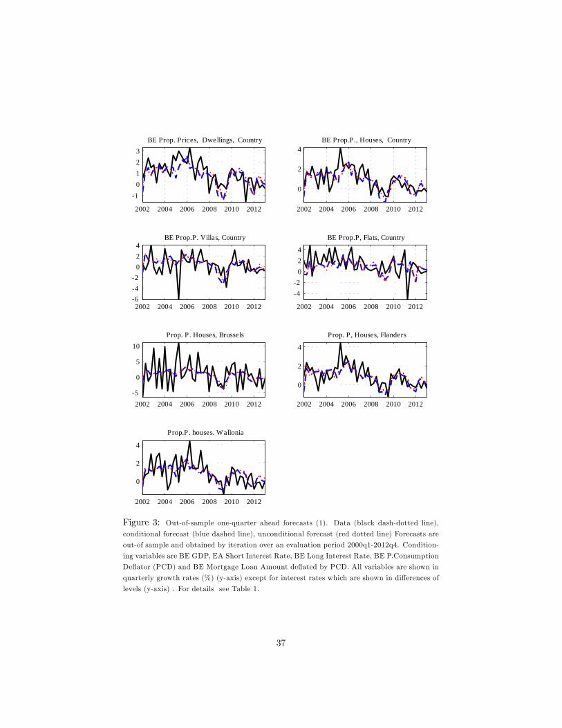
2002 2004 2006 2008 2010 2012

­10123

BE Prop. Prices,  Dwellings,  Country

2002 2004 2006 2008 2010 2012

0

2

4BE Prop.P., Houses,  Country

2002 2004 2006 2008 2010 2012­6­4­2

024

BE Prop.P. Villas, Country

2002 2004 2006 2008 2010 2012

­4­2

024

BE Prop.P, Flats, Country

2002 2004 2006 2008 2010 2012­5

0

5

10Prop. P. Houses, Brussels

2002 2004 2006 2008 2010 2012

0

2

4

Prop. P, Houses, Flanders

2002 2004 2006 2008 2010 2012

0

2

4

Prop.P. houses. Wallonia

Figure 3: Out-of-sample one-quarter ahead forecasts (1). Data (black dash-dotted line),conditional forecast (blue dashed line), unconditional forecast (red dotted line) Forecasts are

out-of sample and obtained by iteration over an evaluation period 2000q1-2012q4. Condition-

ing variables are BE GDP, EA Short Interest Rate, BE Long Interest Rate, BE P.Consumption

De�ator (PCD) and BE Mortgage Loan Amount de�ated by PCD. All variables are shown in

quarterly growth rates (%) (y-axis) except for interest rates which are shown in di¤erences of

levels (y-axis) . For details see Table 1.

37

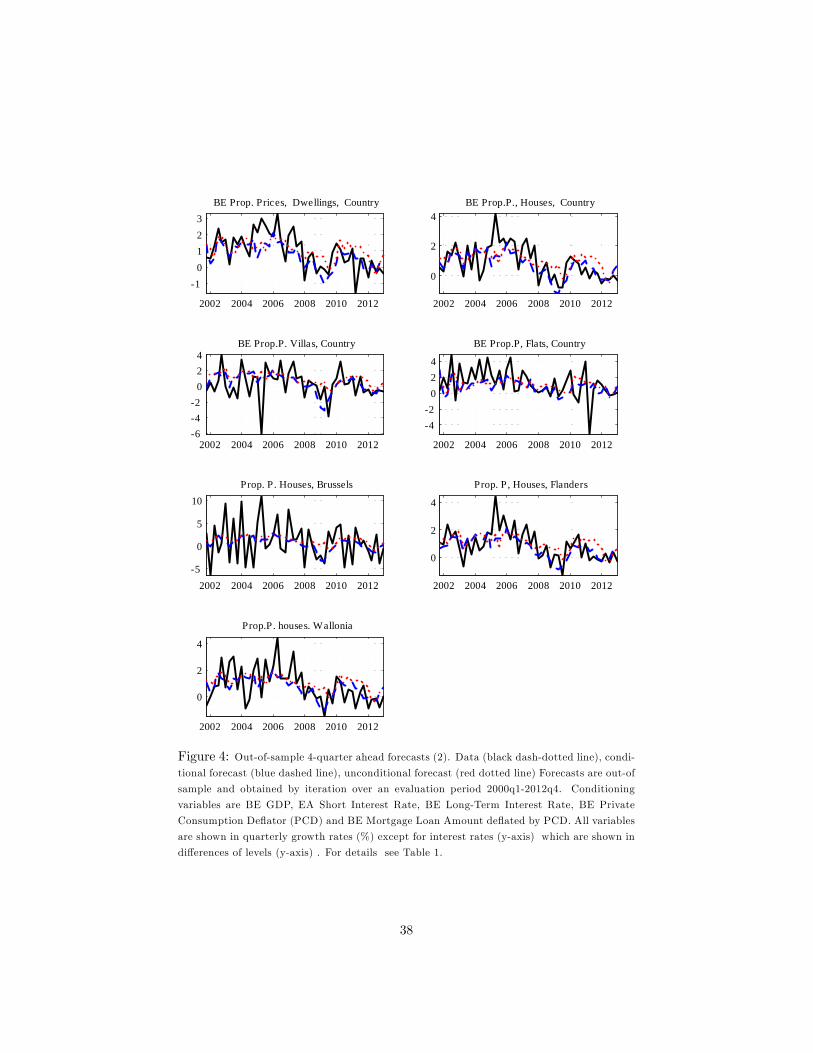
2002 2004 2006 2008 2010 2012

­10123

BE Prop. Prices,  Dwellings,  Country

2002 2004 2006 2008 2010 2012

0

2

4BE Prop.P., Houses,  Country

2002 2004 2006 2008 2010 2012­6­4­2

024

BE Prop.P. Villas, Country

2002 2004 2006 2008 2010 2012

­4­2

024

BE Prop.P, Flats, Country

2002 2004 2006 2008 2010 2012­5

0

5

10Prop. P. Houses, Brussels

2002 2004 2006 2008 2010 2012

0

2

4

Prop. P, Houses, Flanders

2002 2004 2006 2008 2010 2012

0

2

4

Prop.P. houses. Wallonia

Figure 4: Out-of-sample 4-quarter ahead forecasts (2). Data (black dash-dotted line), condi-tional forecast (blue dashed line), unconditional forecast (red dotted line) Forecasts are out-of

sample and obtained by iteration over an evaluation period 2000q1-2012q4. Conditioning

variables are BE GDP, EA Short Interest Rate, BE Long-Term Interest Rate, BE Private

Consumption De�ator (PCD) and BE Mortgage Loan Amount de�ated by PCD. All variables

are shown in quarterly growth rates (%) except for interest rates (y-axis) which are shown in

di¤erences of levels (y-axis) . For details see Table 1.

38

2002 2004 2006 2008 2010 2012­2

­1

0

1

BE  GDP

2002 2004 2006 2008 2010 2012

­0.5

0

0.5

1BE Private consumption

2002 2004 2006 2008 2010 2012

­2

0

2

4

BE Investm ent

2002 2004 2006 2008 2010 2012­10

­5

0

BE  Exports

2002 2004 2006 2008 2010 2012

­4

­2

0

2

BE Residential Investm ent

2002 2004 2006 2008 2010 2012­1

­0.5

0

0.5

BE HICP

2002 2004 2006 2008 2010 2012­0.5

0

0.5

BE  P. Consum ption Deflator

2002 2004 2006 2008 2010 2012

­2

0

2

4

BE Mortgage Credit

Figure 5: Out-of-sample 1-quarter ahead forecasts (3) . Data (black dash-dotted line), condi-tional forecast (blue dashed line), unconditional forecast (red dotted line) Forecasts are out-of

sample and obtained by iteration over an evaluation period 2000q1-2012q4. Conditioning

variables are BE GDP, EA Short Interest Rate, BE Long Interest Rate, BE P.Consumption

De�ator (PCD) and BE Mortgage Loan Amount de�ated by PCD. All variables are shown in

quarterly growth rates (%) (y-axis) except for interest rates which are shown in di¤erences

of levels (y-axis) . For details see Table 1.

39

2002 2004 2006 2008 2010 2012­2

­1

0

1

BE  GDP

2002 2004 2006 2008 2010 2012­0.5

0

0.5

1BE Private consumption

2002 2004 2006 2008 2010 2012

­2

0

2

4

BE Investm ent

2002 2004 2006 2008 2010 2012­10

­5

0

BE  Exports

2002 2004 2006 2008 2010 2012­4

­2

0

2

BE Residential Investm ent

2002 2004 2006 2008 2010 2012­1

­0.5

0

0.5

BE HICP

2002 2004 2006 2008 2010 2012

­0.5

0

0.5

BE  P. Consum ption Deflator

2002 2004 2006 2008 2010 2012

­2

0

2

4

BE Mortgage Credit

Figure 6: Out-of-sample 4 quarter-ahead forecasts (4). Data (black dash-dotted line), condi-tional forecast (blue dashed line), unconditional forecast (red dotted line) Forecasts are out-of

sample and obtained by iteration over an evaluation period 2000q1-2012q4. Conditioning

variables are BE GDP, EA Short Interest Rate, BE Long Interest Rate, BE P.Consumption

De�ator (PCD) and BE Mortgage Loan Amount de�ated by PCD. All variables are shown in

quarterly growth rates (%) (y-axis) except for interest rates which are shown in di¤erences

of levels (y-axis) . For details see Table 1.

40

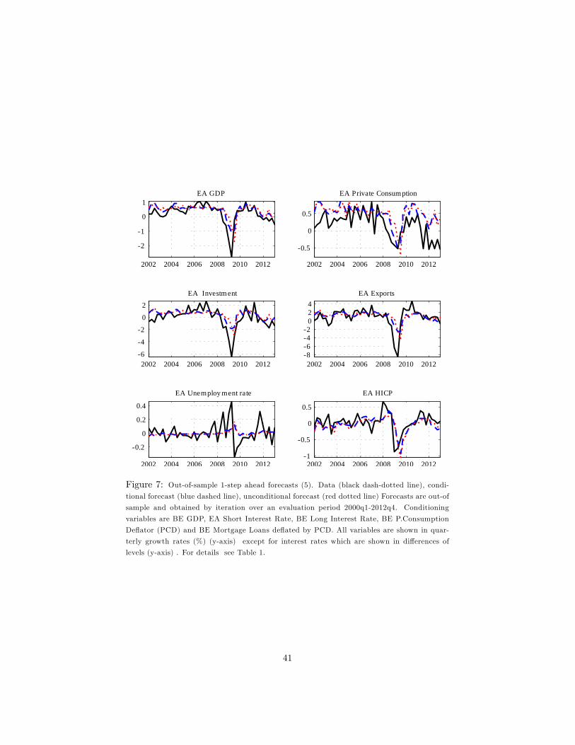
2002 2004 2006 2008 2010 2012

­2

­1

0

1EA GDP

2002 2004 2006 2008 2010 2012

­0.5

0

0.5

EA Private Consum ption

2002 2004 2006 2008 2010 2012­6

­4

­2

0

2EA  Investm ent

2002 2004 2006 2008 2010 2012­8­6­4­2

024

EA Exports

2002 2004 2006 2008 2010 2012

­0.2

0

0.2

0.4

EA Unemploy ment rate

2002 2004 2006 2008 2010 2012­1

­0.5

0

0.5

EA HICP

Figure 7: Out-of-sample 1-step ahead forecasts (5). Data (black dash-dotted line), condi-tional forecast (blue dashed line), unconditional forecast (red dotted line) Forecasts are out-of

sample and obtained by iteration over an evaluation period 2000q1-2012q4. Conditioning

variables are BE GDP, EA Short Interest Rate, BE Long Interest Rate, BE P.Consumption

De�ator (PCD) and BE Mortgage Loans de�ated by PCD. All variables are shown in quar-

terly growth rates (%) (y-axis) except for interest rates which are shown in di¤erences of

levels (y-axis) . For details see Table 1.

41

2002 2004 2006 2008 2010 2012

­2

­1

0

1EA GDP

2002 2004 2006 2008 2010 2012­0.5

0

0.5

EA Private Consum ption

2002 2004 2006 2008 2010 2012­6

­4

­2

0

2

EA  Investm ent

2002 2004 2006 2008 2010 2012­8­6­4­2

024

EA Exports

2002 2004 2006 2008 2010 2012

­0.2

0

0.2

0.4

EA Unemploy ment rate

2002 2004 2006 2008 2010 2012

­1

­0.5

0

0.5

EA HICP

Figure 8: Out-of-sample 4-step ahead forecasts (6). Data (black dash-dotted line), condi-tional forecast (blue dashed line), unconditional forecast (red dotted line) Forecasts are out-of

sample and obtained by iteration over an evaluation period 2002q1-2012q4. Conditioning

variables are BE GDP, EA Short Interest Rate, BE Long Interest Rate, BE P.Consumption

De�ator (PCD) and BE Mortgage Loans de�ated by PCD. All variables are shown in quar-

terly growth rates (%) (y-axis) except for interest rates which are shown in di¤erences of

levels (y-axis) . For details see Table 1.

42

2002 2004 2006 2008 2010 2012­2

­1

0

EA Short­Term  IR

2002 2004 2006 2008 2010 2012

­0.5

0

0.5

BE Long­term  IR

2002 2004 2006 2008 2010 2012

­0.5

0

0.5EA Long­term  IR

2002 2004 2006 2008 2010 2012

­0.6­0.4­0.2

00.2

BE Mortgage IR

2002 2004 2006 2008 2010 2012

­0.5

0

0.5GER 10­y ear Bond Yield

Figure 9: Out-of-sample 1-step ahead forecasts (7). Data (black dash-dotted line), condi-tional forecast (blue dashed line), unconditional forecast (red dotted line) Forecasts are out-of

sample and obtained by iteration over an evaluation period 2000q1-2012q4. Conditioning

variables are BE GDP, EA Short Interest Rate, BE Long Interest Rate, BE P.Consumption

De�ator (PCD) and BE Mortgage Loans de�ated by PCD. All variables are shown in quar-

terly growth rates (%) (y-axis) except for interest rates which are shown in di¤erences of levels

(y-axis) . For details see Table 1.

43

2002 2004 2006 2008 2010 2012­2

­1

0

EA Short­Term  IR

2002 2004 2006 2008 2010 2012

­0.5

0

0.5

BE Long­term  IR

2002 2004 2006 2008 2010 2012­0.5

0

0.5EA Long­term  IR

2002 2004 2006 2008 2010 2012­0.6

­0.4­0.2

0

0.2

BE Mortgage IR

2002 2004 2006 2008 2010 2012

­0.5

0

0.5GER 10­y ear Bond Yield

Figure 10: Out-of-sample 4-step ahead forecasts (8). Data (black dash-dotted line), condi-tional forecast (blue dashed line), unconditional forecast (red dotted line) Forecasts are out-of

sample and obtained by iteration over an evaluation period 2000q1-2012q4. Conditioning

variables are BE GDP, EA Short Interest Rate, BE Long Interest Rate, BE P.Consumption

De�ator (PCD) and BE Mortgage Loan Amount de�ated by PCD. All variables are shown in

quarterly growth rates (%) (y-axis) except for interest rates which are shown in di¤erences

of levels (y-axis) . For details see Table 1.

44

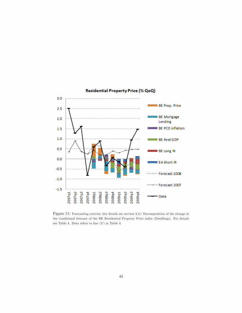
Figure 11: Forecasting exercise (for details see section 3.4): Decomposition of the change inthe conditional forecast of the BE Residential Property Price index (Dwellings). For details

see Table 4. Data refers to line (3�) in Table 4.

45

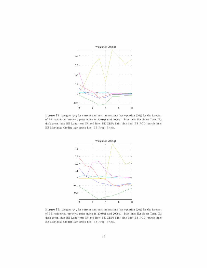
0 2 4 6 8

­0.2

0

0.2

0.4

0.6

0.8

Weights in 2008q1

Figure 12: Weights ij for current and past innovations (see equation (20)) for the forecastof BE residential property price index in 2008q1 and 2009q1. Blue line: EA Short-Term IR;

dark green line: BE Long-term IR; red line: BE GDP; light blue line: BE PCD; purple line:

BE Mortgage Credit; light green line: BE Prop. Prices.

0 2 4 6 8

­0.2

­0.1

0

0.1

0.2

0.3

0.4

Weights in 2009q1

Figure 13: Weights ij for current and past innovations (see equation (20)) for the forecastof BE residential property price index in 2008q1 and 2009q1. Blue line: EA Short-Term IR;

dark green line: BE Long-term IR; red line: BE GDP; light blue line: BE PCD; purple line:

BE Mortgage Credit; light green line: BE Prop. Prices.

46

NBB WORKING PAPER No. 313 – NOVEMBER 2016 47

NATIONAL BANK OF BELGIUM - WORKING PAPERS SERIES The Working Papers are available on the website of the Bank: http://www.nbb.be. 276. “How do exporters react to changes in cost competitiveness?, by S. Decramer, C. Fuss and J. Konings,

Research series, January 2015. 277. “Optimal monetary policy response to endogenous oil price fluctuations”, by A. Stevens, Research series,

January 2015. 278. “Comparing fiscal multipliers across models and countries in Europe”, by J. Kilponen, M. Pisani,

S. Schmidt, V. Corbo, T. Hledik, J. Hollmayr, S. Hurtado, P. Júlio, D. Kulikov, M. Lemoine, M. Lozej, H. Lundvall, J. R. Maria, B. Micallef, D. Papageorgiou, J. Rysanek, D. Sideris, C. Thomas and G. de Walque, Research series, March 2015.

279. “Assessing European competitiveness: The new CompNet micro-based database”, by P. Lopez-Garcia, F. di Mauro and the CompNet Task Force, Research series, April 2015.

280. “FloGARCH: Realizing long memory and asymmetries in returns volatility”, by H. Vander Elst, Research series, April 2015.

281. “Does education raise productivity and wages equally? The moderating roles of age, gender and industry”, by F. Rycx, Y. Saks and I. Tojerow, Research series, April 2015.

282. “Assessing European firms’ exports and productivity distributions: The CompNet trade module”, by A. Berthou, E. Dhyne, M. Bugamelli, A.-M. Cazacu, C.-V. Demian, P. Harasztosi, T. Lalinsky, J. Merikül, F. Oropallo and A. C. Soares, Research series, May 2015.

283. “Economic importance of the Belgian ports: Flemish maritime ports, Liège port complex and the port of Brussels - Report 2013”, by F. Van Nieuwenhove, Document series, June 2015.

284. “Crisis-proof services: Why trade in services did not suffer during the 2008-2009 collapse”, by A. Ariu, Research series, July 2015.

285. “The labour market position of second-generation immigrants in Belgium”, by V. Corluy, J. Haemels, I. Marx and G. Verbist, Research series, September 2015.

286. “The implications of household size and children for life-cycle saving”, by B. Capéau and B. De Rock, Research series, September 2015.

287. “Monetary policy effects on bank risk taking”, by A. Abbate and D. Thaler, Research series, September 2015.

288. “The Belgian production network 2002-2012”, by E. Dhyne, G. Magerman and S. Rubínová, Research series, October 2015.

289. “Portfolio choice and investor preferences: A semi-parametric approach based on risk horizon”, by G. Hübner and T. Lejeune, Research series, October 2015.

290. “Predicting Belgium’s GDP using targeted bridge models”, by Ch. Piette, Research series, January 2016. 291. “Did export promotion help firms weather the crisis?”, by J. Van Biesebroeck, J. Konings and C. Volpe

Martincus, Research series, January 2016. 292. “On the role of public policies and wage formation for business investment in R&D: A long-run panel

analysis”, by T. Buyse, F. Heylen and R. Schoonackers, Research series, January 2016. 293. “Unraveling firms: Demand, productivity and markups heterogeneity”, by E. Forlani, R. Martin, G. Mion and

M. Muûls, Research series, February 2016. 294. “Unemployment risk and over-indebtedness: A micro-econometric perspective”, by Ph. Du Caju, F. Rycx

and I. Tojerow, Research series, February 2016. 295. “International shocks and domestic prices: How large are strategic complementarities?”, by A. Amiti,

O. Itskhoki and J. Konings, Research series, March 2016. 296. “The supplier network of exporters: Connecting the dots”, by E. Dhyne and S. Rubínová, Research series,

May 2016. 297. “Does one size fit all at all times? The role of country specificities and state dependencies in predicting

banking crises” by S. Ferrari and M. Pirovano, Research series, May 2016. 298. “Competition and product mix adjustment of multi-product exporters: Evidence from Belgium”, by

K. Breemersch, Research series, June 2016. 299. “Flemish maritime ports, Liège port complex and the port of Brussels – Report 2014”, by G. Van Gastel,

Document series, June 2016. 300. “Misalignment of productivity and wages across regions? Evidence from Belgian matched panel data”, by

F. Rycx, Y. Saks and I. Tojerow, Research series, July 2016. 301. “The European Payments Union and the origins of Triffin’s regional approach towards international

monetary integration”, by I. Maes and I. Pasotti, Research series, September 2016. 302. “The transmission mechanism of credit support policies in the Euro Area”, by J. Boeckx, M. de Sola Perea

and G. Peersman, Research series, October 2016.

NBB WORKING PAPER No. 313 – NOVEMBER 2016 48

303. “Bank capital (requirements) and credit supply: Evidence from pillar 2 decisions”, by O. De Jonghe, H. Dewachter and S. Ongena, Research series, October 2016.

304. “Monetary and macroprudential policy games in a monetary union”, by R. Dennis and P. Ilbas, Research series, October 2016.

305. “Forward guidance, quantitative easing, or both?, by F. De Graeve and K. Theodoridis, Research series, October 2016.

306. “The impact of sectoral macroprudential capital requirements on mortgage loan pricing: Evidence from the Belgian risk weight add-on”, by S. Ferrari, M. Pirovano and P. Rovira Kaltwasser, Research series, October 2016.

307. “Assessing the role of interbank network structure in business and financial cycle analysis”, by J-Y Gnabo and N.K. Scholtes, Research series, October 2016.

308. “The trade-off between monetary policy and bank stability”, by M. Lamers, F. Mergaerts, E. Meuleman and R. Vander Vennet, Research series, October 2016.

309. “The response of euro area sovereign spreads to the ECB unconventional monetary policies”, by H. Dewachter, L. Iania and J-C. Wijnandts, Research series, October 2016.

310. “The interdependence of monetary and macroprudential policy under the zero lower bound”, by V. Lewis and S. Villa, Research series, October 2016.

311. “The impact of exporting on SME capital structure and debt maturity choices”, by E. Maes, N. Dewaelheynes, C. Fuss and C. Van Hulle, Research series, October 2016.

312. “Heterogeneous firms and the micro origins of aggregate fluctuations”, by G. Magerman, K. De Bruyne, E. Dhyne and J. Van Hove, Research series, October 2016.

313 “A dynamic factor model for forecasting house prices in Belgium”, by M. Emiris, Research series, November 2016.

© Illustrations : National Bank of Belgium

Layout : Analysis and Research Group Cover : NBB AG – Prepress & Image

Published in November 2016

Editor

Jan SmetsGovernor of the National Bank of Belgium

National Bank of Belgium Limited liability company RLP Brussels – Company’s number : 0203.201.340 Registered office : boulevard de Berlaimont 14 – BE -1000 Brussels www.nbb.be