A Distributed Method for Fitting Laplacian RegularizedStratified Models

Jonathan Tuck Shane Barratt Stephen Boyd

September 11, 2019

Abstract

Stratified models are models that depend in an arbitrary way on a set of selectedcategorical features, and depend linearly on the other features. In a basic and tra-ditional formulation a separate model is fit for each value of the categorical feature,using only the data that has the specific categorical value. To this formulation weadd Laplacian regularization, which encourages the model parameters for neighboringcategorical values to be similar. Laplacian regularization allows us to specify one ormore weighted graphs on the stratification feature values. For example, stratifyingover the days of the week, we can specify that the Sunday model parameter shouldbe close to the Saturday and Monday model parameters. The regularization improvesthe performance of the model over the traditional stratified model, since the model foreach value of the categorical ‘borrows strength’ from its neighbors. In particular, itproduces a model even for categorical values that did not appear in the training dataset.

We propose an efficient distributed method for fitting stratified models, based on thealternating direction method of multipliers (ADMM). When the fitting loss functionsare convex, the stratified model fitting problem is convex, and our method computesthe global minimizer of the loss plus regularization; in other cases it computes a lo-cal minimizer. The method is very efficient, and naturally scales to large data setsor numbers of stratified feature values. We illustrate our method with a variety ofexamples.

1 Introduction

We consider the problem of fitting a model to some given data. One common and simpleparadigm parametrizes the model by a parameter vector θ, and uses convex optimizationto minimize an empirical loss on the (training) data set plus a regularization term that(hopefully) skews the model parameter toward one for which the model generalizes to newunseen data. This method usually includes one or more hyper-parameters that scale termsin the regularization. For each of a number of values of the hyper-parameters, a modelparameter is found, and the resulting model is tested on previously unseen data. Among

1

these models, we choose one that achieves a good fit on the test data. The requirement thatthe loss function and regularization be convex limits how the features enter into the model;generally, they are linear (or affine) in the parameters. One advantage of such models is thatthey are generally interpretable.

Such models are widely used, and often work well in practice. Least squares regression[1, 2], lasso [3], logistic regression [4], support vector classifiers [5] are common methodsthat fall into this category (see [6] for these and others). At the other extreme, we canuse models that in principle fit arbitrary nonlinear dependence on the features. Popularexamples include tree based models [7] and neural networks [8].

Stratification is a method to build a model of some data that depends in an arbitraryway on one or more of the categorical features. It identifies one or more categorical featuresand builds a separate model for the data that take on each of the possible values of thesecategorical features.

In this paper we propose augmenting basic stratification with an additional regularizationterm. We take into account the usual loss and regularization terms in the objective, plusan additional regularization term that encourages the parameters found for each value tobe close to their neighbors on some specified weighted graph on the categorical values. Weuse the simplest possible term that encourages closeness of neighboring parameter values:a graph Laplacian on the stratification feature values. (As we will explain below, severalrecent papers use more sophisticated regularization on the parameters for different values ofthe categorical.) We refer to a startified model with this objective function as a Laplacianregularized stratified model. Laplacian regularization can also be interpreted as a prior thatour model parameters vary smoothly across the graph on the stratification feature values.

Stratification (without the Laplacian regularization) is an old and simple idea: Simplyfit a different model for each value of the categorical used to stratify. As a simple examplewhere the data are people, we can stratify on sex, i.e., fit a separate model for females andmales. (Whether or not this stratified model is better than a common model for both femalesand males is determined by out-of-sample or cross-validation.) To this old idea, we add anadditional term that penalizes deviations between the model parameters for females andmales. (This Laplacian regularization would be scaled by a hyper-parameter, whose value ischosen by validation on unseen or test data.) As a simple extension of the example mentionedabove, we can stratify on sex and age, meaning we have a separate model for females andmales, for each age from 1 to 100 (say). Thus we would create a total of 200 differentmodels: one for each age/sex pair. The Laplacian regularization that we add encourages,for example, the model parameters for 37 year old females to be close to that for 37 yearold males, as well as 36 and 38 year old females. We would have two hyper-parameters, onethat scales the deviation of the model coefficients across sex, and another that scales thedeviation of the model coefficients across adjacent ages. One would choose suitable valuesof these hyper-parameters by validation on a test set of data.

There are many other applications where a Laplacian regularized stratified model offers asimple and interpretable model. We can stratify over time, which gives time-varying models,with regularization that encourages our time-dependent model parameters to vary slowly

2

over time. We can capture multiple periodicities in time-varying models, for example byasserting that the 11PM model parameter should be close to the midnight model parameter,the Tuesday and Wednesday parameters should be close to each other, and so on. We canstratify over space, after discretizing location. The Laplacian regularization in this caseencourages the model parameters to vary smoothly over space. This idea naturally falls inline with Waldo Tobler’s “first law of geography” [9]:

Everything is related to everything else, but near things are more related thandistant things.

Compared to simple stratified models, our Laplacian regularized stratified models haveseveral advantages. Without regularization, stratification is limited by the number of datapoints taking each value of the stratification feature, and of course fails (or does not performwell) when there are no data points with some value of the stratification feature. Withregularization there is no such limit; we can even build a model when the training datahas no points with some values of the stratification feature. In this case the model borrowsstrength from its neighbors. Continuing the example mentioned above, we can find a modelfor 37 year old females, even when our data set contains none. Unsurprisingly, the parameterfor 37 year old females is a weighted average of the parameters for 36 and 38 year old females,and 37 year old males.

We can think of stratified models as a hybrid of complex and simple models. The stratifiedmodel has arbitrary dependence on the stratification feature, but simple (typically linear)dependence on the other features. It is essentially non-parametric in the stratified feature,and parametric with a simple form in the other features. The Laplacian regularization allowsus to come up with a sensible model with respect to the stratified feature.

The simplest possible stratified model is a constant for each value of the stratificationfeature. In this case the stratified model is nothing more than a fully non-parametric modelof the stratified feature. The Laplacian regularization in this case encourages smoothness ofthe predicted value relative to some graph on the possible stratification feature values. Moresophisticated models predict a distribution of values of some features, given the stratifiedfeature value, or build a stratified regression model, for example.

In this paper, we first describe stratified model fitting with Laplacian regularization asa convex optimization problem, with one model parameter vector for every value of thestratification feature. This problem is convex (when the loss and regularizers in the fittingmethod are), and so can be reliably solved [10]. We propose an efficient distributed solutionmethod based on the alternating direction method of multipliers (ADMM) [11], which allowsus to solve the optimization problem in a distributed fashion and at very large scale. Ineach iteration of our method, we fit the models for each value of the stratified feature(independently in parallel), and then solve a number of Laplacian systems (one for eachcomponent of the model parameters, also in parallel). We illustrate the ideas and methodwith several examples.

3

2 Related work

Stratification, i.e., the idea of separately fitting a different model for each value of someparameter, is routinely applied in various practical settings. For example, in clinical trials,participants are often divided into subgroups, and one fits a separate model for the datafrom each subgroup [12]. Stratification by itself has immediate benefits; it can be helpfulfor dealing with confounding categorical variables, can help one gain insight into the natureof the data, and can also play a large role in experiment design (see, e.g., [13, 14] for someapplications to clinical research, and [15] for an application to biology).

The idea of adding regularization to fitting stratified models, however, is (unfortunately)not as well known in the data science, machine learning, and statistics communities. In thissection, we outline some ideas related to stratified models, and also outline some prior workon Laplacian regularization.

Regularized lasso models. The data-shared lasso is a stratified model that encouragescloseness of parameters by their difference as measured by the `1-norm [16]. (Laplacianregularization penalizes their difference by the `2-norm squared.) The pliable lasso is a gen-eralization of the lasso that is also a stratified model, encouraging closeness of parametersas measured by a blend of the `1- and `2-norms [17, 18]. The network lasso is a stratifiedmodel that encourages closeness of parameters by their difference as measured by the `2-norm[19, 20]. The network lasso problem results in groups of models with the same parameters,in effect clustering the stratification features. (In contrast, Laplacian regularization leadsto smooth parameter values.) The ideas in the original papers on the network lasso werecombined and made more general, resulting in the software package SnapVX [21], a generalsolver for convex optimization problems defined on graphs that is based on SNAP [22] andcvxpy [23]. One could, in principle, implement Laplacian regularized stratified models inSnapVX; instead we develop specialized methods for the specific case of Laplacian regular-ization, which leads to faster and more robust methods. We also have observed that, in mostpractical settings, Laplacian regularization is all you need.

Varying-coefficient models. Varying-coefficient models are a class of regression and clas-sification models in which the model parameters are smooth functions of some features [24].A stratified model can be thought of as a special case of varying-coefficient models, wherethe features used to choose the coefficients are categorical. Estimating varying-coefficientmodels is generally nonconvex and computationally expensive [25].

Geographically weighted regression. The method of geographically weighted regres-sion (GWR) is widely used in the field of geographic information systems (GIS). It consistsof a spatially-varying linear model with a location attribute [26]. GWR fits a model for eachlocation using every data point, where each data point is weighted by a kernel function ofthe pairwise locations. (See, e.g., [27] for a recent survey and applications.) GWR is an ex-tremely special case of a stratified model, where the task is regression and the stratification

4

feature is location.

Graph-based feature regularization. One can apply graph regularization to the fea-tures themselves. For example, the group lasso penalty enforces sparsity of model coefficientsamong groups of features [28, 29], performing feature selection at the level of groups of fea-tures. The group lasso is often fit using a method based on ADMM, which is similar in veinto the one we describe. The group lasso penalty can be used as a regularization term toany linear model, e.g., logistic regression [30]. A related idea is to use a Laplacian regular-ization term on the features, leading to, e.g., Laplacian regularized least-squares (LapRLS)and Laplacian regularized support vector machines (LapSVM) [31]. Laplacian regularizedmodels have been applied to many disciplines and fields, e.g., to semi-supervised learning[32, 33], communication [34, 35, 36], medical imaging [37], computer vision [38], naturallanguage processing [39], and microbiology [40].

Graph interpolation. In graph interpolation or regression on a graph, one is given vectorsat some of the vertices of a graph, and is tasked with inferring the vectors at the other(unknown) vertices [41]. This can be viewed as a stratified model where the parameter ateach vertex or node is a constant. This leads to, e.g., the total variation denoising problemin signal processing [42].

Multi-task learning. In multi-task learning, the goal is to learn models for multiplerelated tasks by taking advantage of pair-wise relationships between the tasks (see, e.g.,[43, 44]). Multi-task learning can be interpreted as a stratified model where the stratificationfeature is the task to be performed by that model. Laplacian regularization has also beeninvestigated in the context of multi-task learning [45].

Laplacian systems. Laplacian matrices are very well studied in the field of spectral graphtheory [46, 47]. A set of linear equations with Laplacian coefficient matrix is called a Lapla-cian system. Many problems give rise to Laplacian systems, including in electrical engineer-ing (resistor networks), physics (vibrations and heat), computer science, and spectral graphtheory (see, e.g., [48] for a survey). While solving a general linear system requires order K3

flops, where K is the number of vertices in the graph, Laplacian system solvers have beendeveloped that are (nearly) linear in the number of edges contained in the associated graph[49, 50, 51]. In many cases, however, the graph can be large and dense enough that solvinga Laplacian system is still a highly nontrivial computational issue; in these cases, graphsparsification can be used to yield results of moderate accuracy in much less time [52]. Inpractice, the conjugate gradient (CG) method [53], with a suitable pre-conditioner, can beextremely efficient for solving the (positive definite) Tikhonov-regularized Laplacian systemsthat we encounter in this paper.

Laplacian regularized minimization problems. Stratified model fitting with Lapla-cian regularization is simply a convex optimization problem with Laplacian regularization.

5

There are many general-purpose methods that solve this problem, indeed too many to name;in this paper we derive a problem-specific algorithm using ADMM. Another possibility wouldbe majorization-minimization (MM), an algorithmic framework where one iteratively mini-mizes a majorizer of the original function at the current iterate [54]. One possible majorizerfor the Laplacian regularization term is a diagonal quadratic, allowing block separable prob-lems to be solved in parallel; this was done in [55]. The MM and ADMM algorithms havebeen shown to be closely connected [56], since the proximal operator of a function minimizesa quadratic majorizer. However, convergence with MM depends heavily on the choice of ma-jorizer and the problem structure [57]. In contrast, the ADMM-based algorithm we describein this paper typically converges (at least to reasonable practical tolerance) within 100–200iterations.

3 Stratified models

In this section we define stratified models and our fitting method; we describe our distributedmethod for carrying out the fitting in §4.

We consider data fitting problems with items or records of the form (z, x, y) ∈ Z×X ×Y .Here z ∈ Z is the feature over which we stratify, x ∈ X is the other features, and y ∈ Y is theoutcome or dependent variable. For our purposes, it does not matter what X or Y are; theycan consist of numerical, categorical, or other data types. The stratified feature values Z,however, must consist of only K possible values, which we denote as Z = {1, . . . , K}. Whatwe call z can include several original features, for example, sex and age. If all combinationsof these original features are possible, then K is the product of the numbers of values thesefeatures can take on. In some formulations, described below, we do not have x; in this case,the records have the simplified form (z, y).

Base model. We build a stratified model on top of a base model, which models pairs(x, y) (or, when x is absent, just y). The base model is parametrized by a parameter vectorθ ∈ Θ ⊆ Rn. In a stratified model, we use a different value of the parameter θ for each valueof z. We denote these parameters as θ1, . . . , θK , where θk is the parameter value used whenz = k. We let θ = (θ1, . . . , θK) ∈ RKn denote the collection of parameter values, i.e., theparameter value for the stratified model.

Local loss and regularization. Let (zi, xi, yi), i = 1 . . . , N , denote a set of N trainingdata points or examples. We will use regularized empirical loss minimization to choose theparameters θ1, . . . , θK . Let l : Θ×X ×Y → R be a loss function. We define the kth (local)empirical loss as

`k(θ) =∑i:zi=k

l(θ, xi, yi) (1)

(without xi when x is absent).We may additionally add a regularizer to the local loss function. The idea of regularization

can be traced back to as early as the 1940s, where it was introduced as a method to stabilize

6

ill-posed problems [58, 59]. Let r : Θ→ R∪{∞} be a regularization function or regularizer.Choosing θk to minimize `k(θk) + r(θk) gives the regularized empirical risk minimizationmodel parameters, based only on the data records that take the particular value of thestratification feature z = k. This corresponds to the traditional stratified model, with noconnection between the parameter values for different values of z. (Infinite values of theregularizer encode constraints on allowable model parameters.)

Laplacian regularization. Let W ∈ RK×K be a symmetric matrix with nonnegativeentries. The associated Laplacian regularization is the function L : RKn → R given by

L(θ) = L(θ1, . . . , θK) =1

2

K∑i,j=1

Wij‖θi − θj‖22. (2)

(To distinguish the Laplacian regularization L from r in (1), we refer to r as the localregularization.) We can associate the Laplacian regularization with a graph with K vertices,which has an edge (i, j) for each positive Wij, with weight Wij. We refer to this graphas the regularization graph. We can express the Laplacian regularization as the positivesemidefinite quadratic form

L(θ) = (1/2)θT (I ⊗ L)θ,

where ⊗ denotes the Kronecker product, and L ∈ RK×K is the (weighted) Laplacian matrixassociated with the weighted graph, given by

Lij =

{ −Wij i 6= j∑Kk=1Wik i = j

for i, j = 1, . . . , K.The Laplacian regularization L(θ) evidently measures the aggregate deviation of the pa-

rameter vectors from their graph neighbors, weighted by the edge weights. Roughly speaking,it is a metric of how rough or non-smooth the mapping from z to θz is, measured by theedge weights.

Fitting the stratified model. To choose the parameters θ1, . . . , θK , we minimize

F (θ1, . . . , θk) =K∑k=1

(`k(θk) + r(θk)) + L(θ1, . . . , θK). (3)

The first term is the sum of the local objective functions, used in fitting a traditional stratifiedmodel; the second measures the non-smoothness of the model parameters as measured bythe Laplacian. It encourages parameter values for neighboring values of z to be close to eachother.

7

Convexity assumption. We will assume that the local loss function l(θ, x, y) and thelocal regularizer r(θ) are convex functions of θ, which implies that that the local losses `k areconvex functions of θ. The Laplacian is also convex, so the overall objective F is convex, andminimizing it (i.e., fitting a stratified model) is a convex optimization problem. In §4 we willdescribe an effective distributed method for solving this problem. (Much of our developmentcarries over to the case when l or r is not convex; in this case, of course, we can only expectto find a local minimizer of F ; see §6.)

The two extremes. Assuming the regularization graph is connected, taking the positiveweights Wij to ∞ forces all the parameters to be equal, i.e., θ1 = · · · = θK . We refer tothis as the common model (i.e., one which does not depend on z). At the other extreme wecan take all Wij to 0, which results in a traditional stratified model, with separate modelsindependently fit for each value of z.

Hyper-parameters. The local regularizer and the weight matrix W typically containsome positive hyper-parameters, for example that scale the local regularization or one ormore edges weights in the graph. As usual, these are varied over a range of values, and foreach value a stratified model is found, and tested on a separate validation data set usingan appropriate true objective. We choose values of the hyper-parameters that give goodvalidation set performance; finally, we test this model on a new test data set.

Modeling with no data at nodes. Suppose that at a particular node on the graph (i.e.,value of stratification feature), there is no data to fit a model. Then, the model for thatnode will simply be a weighted average of the models of its neighboring nodes.

3.1 Data models

So far we have been vague about what exactly a data model is. In this section we list just afew of the many possibilities.

3.1.1 Point estimates

The first type of data model that we consider is one where we wish to predict a single likelyvalue, or point estimate, of y for a given x and z. In other words, we want to construct afunction fz : X → Y such that fz(x) ≈ y.

Regression. In a regression data model, X = Rn and Y = R, with one component of xalways having the value one. The loss has the form l(θ, x, y) = p(xT θ−y), where p : R→ R isa penalty function. Some common (convex) choices include the square penalty [1, 2], absolutevalue penalty [60], Huber penalty [61], and tilted absolute value (for quantile regression).Common generic regularizers include zero, sum of squares, and the `1 norm [3]; these typicallydo not include the coefficient in θ associated with the constant feature value one, and are

8

scaled by a positive hyper-parameter. Various combinations of these choices lead to ordinaryleast squares regression, ridge regression, the lasso, Huber regression, and quantile regression.Multiple regularizers can also be employed, each with a different hyper-parameter, as in theelastic net. Constraints on model parameters (for example, nonnegativity) can be imposedby infinite values of the regularizer.

The stratified regression model gives the predictor of y, given z and x, given by

fz(x) = xT θz.

The stratified model uses a different set of regression coefficients for each value of z. Forexample, we can have a stratified lasso model, or a stratified nonnegative least squares model.

An interesting extension of the regression model, sometimes called multivariate or multi-task regression, takes Y = Rm with m > 1. In this case we take Θ = Rn×m, so θz is a matrix,with fz(x) = xT θz as our predictor for y. An interesting regularizer for multi-task regressionis the nuclear norm, which is the sum of singular values, scaled by a hyper-parameter [62].This encourages the matrices θz to have low rank.

Boolean classification. In a boolean classification data model, X = Rn and Y = {−1, 1}.The loss has the form l(θ, x, y) = p(yxT θ), where p : R→ R is a penalty function. Common(convex) choices of p are p(u) = (u − 1)2 (square loss); p(u) = (u − 1)+ (hinge loss), andp(u) = log(1 + exp−u) (logistic loss). The predictor is

fz(x) = sign(xT θz).

The same regularizers mentioned in regression can be used. Various choices of these lossfunctions and regularizers lead to least squares classification, support vector machines (SVM)[63], logistic regression [4, 64], and so on [6]. For example, a stratified SVM model developsan SVM model for each value of z; the Laplacian regularization encourages the parametersassociated with neighboring values of z to be close.

Multi-class classification. Here X = Rn, and Y is finite, say, {1, . . . ,M}. We usuallytake Θ = Rn×M , with associated predictor fz(x) = argmaxi

(xT θz

)i. Common (convex) loss

functions are the multi-class logistic (multinomial) loss [65],

l(θ, x, y) = log

(M∑j=1

exp(xT θ)j

)− (xT θ)y, y = 1, . . . ,M,

and the multi-class SVM loss [66, 67],

l(θ, x, y) =∑i:i 6=y

((xT θ)i − (xT θ)y + 1)+, y = 1, . . . ,M.

The same regularizers mentioned in multivariate regression can be used.

9

Point estimates without x. As mentioned above, x can be absent. In this case, wepredict y given only z. We can also interpret this as a point estimate with an x that isalways constant, e.g., x = 1. In a regression problem without x, the parameter θz is a scalar,and corresponds simply to a prediction of the value y. The loss has the form l(θ, y) = p(θ−y),where p is any of the penalty functions mentioned in the regression section. If, for example, pwere the square (absolute value) penalty, then θk would correspond to the average (median) ofthe yi that take on the particular stratification feature k, or zi = k. In a boolean classificationproblem, θz ∈ R, and the predictor is sign(θz), the most likely class. The loss has the forml(θ, y) = p(yθ), where p is any of the penalty functions mentioned in the boolean classificationsection. A similar predictor can be derived for the case of multi-class classification.

3.1.2 Conditional distribution estimates

A more sophisticated data model predicts the conditional probability distribution of y givenx (rather than a specific value of y given x, in a point estimate). We parametrize thisconditional probability distribution by a vector θ, which we denote as Prob(y | x, θ). Thedata model could be any generalized linear model [68]; here we describe a few common ones.

Logistic regression. Here X = Rn and Y = {−1, 1}, with one component of x alwayshaving the value one. The conditional probability has the form

Prob(y = 1 | x, θ) =1

1 + e−xT θ.

(So Prob(y = −1 | x, θ) = 1 − Prob(y = 1 | x, θ).) The loss, often called the logistic loss,has the form l(θ, x, y) = log(1+exp(−yθTx)), and corresponds to the negative log-likelihoodof the data record (x, y), when the parameter vector is θ. The same regularizers mentioned inregression can be used. Validating a logistic regression data model using the average logisticloss on a test set is the same (up to a constant factor) as the average log probability of theobserved values in the test data, under the predicted conditional distributions.

Multinomial logistic regression. Here X = Rn and Y is finite, say {1, . . . ,M} with onecomponent of x equal to one. The parameter vector is a matrix θ ∈ Rn×M . The conditionalprobability has the form

Prob(y = i | x, θ) =exp(xT θ)i∑Mj=1 exp(xT θ)j

, i = 1, . . . ,M.

The loss has the form

l(θ, x, y = i) = log

(M∑j=1

exp(xT θ)j

)− (xT θ)i, i = 1, . . . ,M,

and corresponds to the negative log-likelihood of the data record (x, y).

10

Exponential regression. Here X = Rn and Y = R+ (i.e., the nonnegative reals). Theconditional probability distribution in exponential regression has the form

Prob(y | x, θ) = exp(xT θ)e− exp(xT θ)y,

where θ ∈ Rn is the parameter vector. This is an exponential distribution over y, with rateparameter given by ω = exp(xT θ). The loss has the form

l(θ, x, y) = −xT θ + exp(xT θ)y,

which corresponds to the negative log-likelihood of the data record (x, y) under the expo-nential distribution with parameter ω = exp(xT θ). Exponential regression is useful whenthe outcome y is positive. A similar conditional probability distribution can be derived forthe other distributions, e.g., the Poisson distribution.

3.1.3 Distribution estimates

A distribution estimate is an estimate of the probability distribution of y when x is absent,denoted p(y | θ). This data model can also be interpreted as a conditional distributionestimate when x = 1. The stratified distribution model consists of a separate distributionfor y, for each value of the stratification parameter z. The Laplacian regularization in thiscase encourages closeness between distributions that have similar stratification parameters,measured by the distance between their model parameters.

Gaussian distribution. Here Y = Rm, and we fit a density to the observed values ofy, given z. For example θ can parametrize a Gaussian on Rm, N (µ,Σ). The standardparametrization uses the parameters θ = (Σ−1,Σ−1µ), with Θ = Sm++ × Rm (Sn++ denotesthe set of n× n positive definite matrices.) The probability density function of y is

p(y | θ) = (2π)−m/2 det(Σ)−1/2 exp(−1

2(y − µ)TΣ−1(y − µ))

The loss function (in the standard parametrization) is

l(θ, y) = − log detS + yTSy − 2yTν + νTS−1ν

where θ = (S, ν) = (Σ−1,Σ−1µ). This loss function is jointly convex in S and ν; the first threeterms are evidently convex and the fourth is the matrix fractional function (see [10, p76]).Some common (convex) choices for the local regularization function include the trace of Σ−1

(encourages the harmonic mean of the eigenvalues of Σ, and hence volume, to be large),sum of squares of Σ−1 (shrinks the overall conditional dependence between the variables),`1-norm of Σ−1 (encourages conditional independence between the variables) [69], or a prioron Σ−1 or Σ−1µ.

When m = 1, this model corresponds to the standard normal distribution, with mean µand variance σ2. A stratified Gaussian distribution model has a separate mean and covari-ance of y for each value of the stratification parameter z. This model can be validated byevaluating the average log density of the observed values yi, under the predicted distributions,over a test set of data.

11

Bernoulli distribution. Here Y = Rn+. The probability density function of a Bernoulli

distribution has the formp(y | θ) = θ1

T y(1− θ)n−1T y,

where θ ∈ Θ = [0, 1]. The loss function has the form

l(θ, y) = −(1Ty) log(θ)− (n− 1Ty) log(1− θ),

which corresponds to the negative log-likelihood of the Bernoulli distribution.

Poisson distribution. Here Y = Z+ (i.e., the nonnegative integers). The probabilitydensity function of a Poisson distribution has the form

p(y = k | θ) =θke−θ

k!, k = 0, 1, . . . ,

where θ ∈ Θ = R+. If θ = 0, then p(y = 0 | θ) = 1. The loss function has the form

l(θ, y = k) = −k log θ + θ, k = 0, 1, . . . ,

which corresponds to the negative log-likelihood of the Poisson distribution. A similar datamodel can be derived for the exponential distribution.

Non-parametric discrete distribution. Here Y is finite, say {1, . . . ,M} where M > 1.We fit a non-parametric discrete distribution to y, which has the form

p(y = k | θ) = θk, k = 1, . . . ,M,

where θ ∈ Θ = {p ∈ RM | 1Tp = 1, p � 0}, i.e., the probability simplex. The loss functionhas the form

l(θ, y = k) = − log(θk), k = 1, . . . ,M.

A common (convex) regularization function is the negative entropy, given by∑M

i=1 θi log(θi).

Exponential families. A probability distribution that can be expressed as

p(y | θ) = eM(θ,y)

where M : Rn × Y → R is a concave function of θ, is an exponential family [70, 71].Some important special cases include the Bernoulli, multinomial, Gaussian, and Poissondistributions. A probability distribution that has this form naturally leads to the following(convex) loss function

l(θ, y) = − log p(y | θ) = −M(θ, y).

12

3.2 Regularization graphs

In this section we outline some common regularization graphs, which are undirected weightedgraphs where each vertex corresponds to a possible value of z. We also detail some possibleuses of each type of regularization graph in stratified model fitting.

Complete graph. A complete graph is a (fully connected) graph that contains everypossible edge. In this case, all of the models for each stratification feature are encouragedto be close to each other.

Star graph. A star graph has one vertex with edges to every other vertex. The vertexthat is connected to every other vertex is sometimes called the internal vertex. In a stratifiedmodel with a star regularization graph, the parameters of all of the non-internal vertices areencouraged to be similar to the parameter of the internal vertex. We refer to the internalvertex as the common model. A common use of a star graph is when the stratification featurerelates many vertices only to the internal vertex.

It is possible to have no data associated with the common model or internal vertex. Inthis case the common model parameter is a weighted average of other model parameters; itserves to pull the other parameter values together.

It is a simple exercise to show that a stratified model with the complete graph can also befound using a star graph, with a central or internal vertex that is connected to all others, buthas no data. (That is, it corresponds to a new fictitious value of the stratification feature,that does not occur in the real data.)

Path graph. A path graph, or linear/chain graph, is a graph whose vertices can be listedin order, with edges between adjacent vertices in that order. The first and last vertices onlyhave one edge, whereas the other vertices have two edges. Path graphs are a natural choicefor when the stratification feature corresponds to time, or location in one dimension. Whenthe stratification feature corresponds to time, a stratified model with a path regularizationgraph correspond to a time-varying model, where the model varies smoothly with time.

Cycle graph. A cycle graph or circular graph is a graph where the vertices are connectedin a closed chain. Every vertex in a cycle graph has two edges. A common use of a cyclegraph is when the stratification feature corresponds to a periodic variables, e.g., the dayof the week; in this case, we fit a separate model for each day of the week, and the modelparameter for Sunday is close to both the model parameter for Monday and the modelparameter for Saturday. Other examples include days of the year, the season, and non-timevariables such as angle.

Tree graph. A tree graph is a graph where any two vertices are connected by exactlyone path (which may consist of multiple edges). Tree graphs can be useful for stratificationfeatures that naturally have hierarchical structure, e.g., the location in a corporate hierarchy,

13

or in finance, hierarchical classification of individual stocks into sectors, industries, and sub-industries. As in the star graph, which is a special case of a tree graph, internal verticesneed not have any data associated with them, i.e., the data is only at the leaves of the tree.

Grid graph. A grid graph is a graph where the vertices correspond to points with integercoordinates, and two vertices are connected if their maximum distance in each coordinate isless than or equal to one. For example, a path graph is a one-dimensional grid graph.

Grid graphs are useful for when the stratification feature corresponds to locations. Wediscretize the locations into bins, and connect adjacent bins in each dimension to create agrid graph. A space-stratified model with grid graph regularization is encouraged to havemodel parameters that vary smoothly through physical space.

Entity graph. There can be a vertex for every value of some entity, e.g., a person. Theentity graph has an edge between two entities if they are perceived to be similar. For example,two people could be connected in a (friendship) entity graph if they were friends on a socialnetworking site. In this case, we would fit a separate model for each person, and encouragefriends to have similar models. We can have multiple relations among the entities, eachone associated with its own graph; these would typically be weighted by separate hyper-parameters.

Products of graphs. As mentioned earlier, z can include several original features, andK, the number of possible values of z, is the product of the number of values that thesefeatures take on. Each original stratification feature can have its own regularization graph,with the resulting regularization graph for z given by the (weighted) Cartesian product ofthe graphs of each of the features. For example, the product of two path graphs is a gridgraph, with the horizontal and vertical edges having different weights, associated with thetwo original stratification features.

4 Distributed method for stratified model fitting

In this section we describe a distributed algorithm for solving the fitting problem (3). Themethod alternates between computing (in parallel) the proximal operator of the local lossand local regularizer for each model, and computing the proximal operator of the Laplacianregularization term, which requires the solution of a number of regularized Laplacian linearsystems (which can also be done in parallel).

To derive the algorithm, we first express (3) in the equivalent form

minimizeK∑k=1

(`k(θk) + r(θk)) + L(θ1, . . . , θK)

subject to θ = θ, θ = θ,

(4)

14

where we have introduced two additional optimization variables θ ∈ RKn and θ ∈ RKn. Theaugmented Lagrangian Lλ of (4) has the form

Lλ(θ, θ, θ, u, u) =K∑k=1

(`k(θk) + r(θk)) + L(θ1, . . . , θK)

+ (1/2λ)‖θ − θ + u‖22 + (1/2λ)‖θ − θ + u‖22,

where u ∈ RKn and u ∈ RKn are the (scaled) dual variables associated with the twoconstraints in (4), respectively, and λ > 0 is the penalty parameter. The ADMM algorithm

(in scaled dual form) for the splitting (θ, θ) and θ consists of the iterations

θi+1, θi+1 := argminθ,θ

Lλ(θ, θ, θi, ui, ui)

θi+1 := argminθ

Lλ(θi, θi, θ, ui, ui)

ui+1 := ui + θi+1 − θi+1

ui+1 := ui + θi+1 − θi+1.

Since the problem is convex, the iterates θi, θi, and θi are guaranteed to converge to eachother and to a primal optimal point of (3) [11].

This algorithm can be greatly simplified (and parallelized) with a few simple observations.Our first observation is that the first step in ADMM can be expressed as

θi+1k = proxλlk(θik − uik), θi+1

k = proxλr(θik − uik), k = 1, . . . , K,

where proxg : Rn → Rn is the proximal operator of the function g [72] (see the Appendix forthe definition and some examples of proximal operators). This means that we can compute

θi+1 and θi+1 at the same time, since they do not depend on each other. Also, we cancompute θi+1

1 , . . . , θi+1K (and θi+1

1 , . . . , θi+1K ) in parallel.

Our second observation is that the second step in ADMM can be expressed as the solutionto the n regularized Laplacian systems

(L+ (2/λ)I

)(θi+1

1 )j(θi+1

2 )j...

(θi+1K )j

= (1/λ)

(θi+1

1 + ui1 + θi+11 + ui1)j

(θi+12 + ui2 + θi+1

2 + ui2)j...

(θi+1K + uiK + θi+1

K + uiK)j

, j = 1, . . . , n. (5)

These systems can be solved in parallel. Many efficient methods for solving these systemshave been developed; we find that the conjugate gradient (CG) method [73], with a diagonalpre-conditioner, can efficiently and reliably solve these systems. (We can also warm-start

CG with θi.) Combining these observations leads to Algorithm 4.1.

Algorithm 4.1 Distributed method for fitting stratified models with Laplacian regularization.

15

given Loss functions `1, . . . , `K , local regularization function r,graph Laplacian matrix L, and penalty parameter λ > 0.

Initialize. θ0 = θ0 = θ0 = u0 = u0 = 0.repeat

in parallel

1. Evaluate proximal operator of lk. θi+1k = proxλ`k(θik − uik), k = 1, . . . ,K

2. Evaluate proximal operator of r. θi+1k = proxλr(θ

ik − uik), k = 1, . . . ,K

3. Solve the regularized Laplacian systems (5) in parallel.

4. Update the dual variables. ui+1 := ui + θi+1 − θi+1; ui+1 := ui + θi+1 − θi+1

until convergence

Evaluating the proximal operator of lk. Evaluating the proximal operator of lk corre-sponds to solving a fitting problem with sum-of-squares regularization. In some cases, thishas a closed-form expression, and in others, it requires solving a small convex optimizationproblem. When the loss is differentiable, we can use, for example, the L-BFGS algorithm tosolve it [74]. (We can also warm start with θi.) We can also re-use factorizations of matrices(e.g., Hessians) used in previous evaluations of the proximal operator.

Evaluating the proximal operator of r. The proximal operator of r often has a closed-form expression. For example, if r(θ) = 0, then the proximal operator of r corresponds tothe projection onto Θ. If r is the sum of squares function and Θ = Rn, then the proximaloperator of r corresponds to the (linear) shrinkage operator. If r is the `1 norm and Θ = Rn,then the proximal operator of r corresponds to soft-thresholding, which can be performed inparallel.

Stopping criterion. The primal and dual residuals

ri+1 = (θi+1 − θi+1, θi+1 − θi+1), si+1 = −(1/λ)(θi+1 − θi, θi+1 − θi),

converge to zero [11]. This suggests the stopping criterion

‖ri+1‖2 ≤ εpri, ‖si+1‖2 ≤ εdual,

where εpri and εdual are given by

εpri =√

2Knεabs + εrel max{‖ri+1‖2, ‖si+1‖2}, εdual =√

2Knεabs + (εrel/λ)‖(ui, ui)‖2,

for some absolute tolerance εabs > 0 and relative tolerance εrel > 0.

Selecting the penalty parameter. Algorithm 4.1 will converge regardless of the choiceof the penalty parameter λ. However, the choice of the penalty parameter can affect the

16

speed of convergence. We adopt the simple adaptive scheme [75, 76]

λk+1 :=

λk/τ incr if ‖rk‖2 > µ‖sk‖2τdecrλk if ‖sk‖2 > µ‖rk‖2λk otherwise,

where µ > 1, τ incr > 1, and τdecr > 1 are parameters. (We recommend µ = 5, τ incr = 2, andτdecr = 2.) We found that this simple scheme with λ0 = 1 worked very well across all of ourexperiments. When λi+1 6= λi, we must re-scale the dual variables, since we are using withscaled dual variables. The re-scaling is given by

ui+1 = cui+1, ui+1 = cui+1,

where c = λi+1/λi.

Regularization path via warm-start. Our algorithm supports warm starting by choos-ing the initial point θ0 as an estimate of the solution, for example, the solution of a closelyrelated problem (e.g., a problem with slightly varying hyper-parameters.)

Software implementation. We provide an (easily extensible) implementation of the ideasdescribed in the paper, available at www.github.com/cvxgrp/strat_models. We use numpy

for dense matrix representation and operations [77], scipy for sparse matrix operationsand statistics functions [78], networkx for graph factory functions and Laplacian matrixcomputation [79], torch for L-BFGS and GPU computation [80], and multiprocessing forparallel processing. We provide implementations of a number of common stratified models,all of which support the method

model.fit(X,Y,Z,G).

Here X, Y , and Z are numpy matrices with the data and stratification features and G is anetworkx graph with nodes corresponding to Z describing the Laplacian. When model isa distribution estimate, its signature is model.fit(Y,Z,G). We also provide methods thatautomatically compute cross validation scores.

We note that our implementation is for the most part expository and for experimentationwith stratified models; its speed could evidently be improved by using a compiled language(e.g., C or C++). Practictioners looking to use these methods at a large scale should developspecialized codes for their particular application using the ideas that we have described.

5 Examples

In this section we illustrate the effectiveness of stratified models by combining base fittingmethods and regularization graphs to create stratified models. We note that these examplesare all highly simplified in order to illustrate their usage; better models can be devised using

17

the very same techniques illustrated. In each example, we fit three models: a stratified modelwithout Laplacian regularization (which we refer to as a separate model), a common modelwithout stratification, and a stratified model with hand-picked edge weights. (In practice theedge weights should be selected using a validation procedure.) We find that the stratifiedmodel significantly outperforms the other two methods in each example.

The code is available online at https://github.com/cvxgrp/strat_models. All nu-merical experiments were performed on an unloaded Intel i7-8700K CPU.

5.1 Mesothelioma classification

We consider the problem of predicting whether a patient has mesothelioma, a form of cancer,given their sex, age, and other medical features that were gathered during a series of patientencounters and laboratory studies.

Dataset. We obtained data describing 324 patients from the Dicle University Faculty ofMedicine [81, 82]. The dataset is comprised of males and females between (and including)the ages of 19 and 85, with 96 (29.6%) of the patients diagnosed with mesothelioma. The32 medical features in this dataset include: city, asbestos exposure, type of MM, durationof asbestos exposure, diagnosis method, keep side, cytology, duration of symptoms, dysp-noea, ache on chest, weakness, habit of cigarette, performance status, white blood cell count(WBC), hemoglobin (HGB), platelet count (PLT), sedimentation, blood lactic dehydrogenise(LDH), alkaline phosphatise (ALP), total protein, albumin, glucose, pleural lactic dehydro-genise, pleural protein, pleural albumin, pleural glucose, dead or not, pleural effusion, pleuralthickness on tomography, pleural level of acidity (pH), C-reactive protein (CRP), class ofdiagnosis (whether or not the patient has mesothelioma). We randomly split the data intoa training set containing 90% of the records, and a test set containing the remaining 10%.

Data records. The ‘diagnosis method’ feature is perfectly correlated with the output,so we removed it (this was not done in many other studies on this dataset which led tonear-perfect classifiers). We performed rudimentary feature engineering on the raw medicalfeatures to derive a feature vector x ∈ R46. The outcomes y ∈ {0, 1} denote whetheror not the patient has mesothelioma, with y = 1 meaning the patient has mesothelioma.The stratification feature z is a tuple consisting of the patient’s sex and age; for example,z = (Male, 62) corresponds to a 62 year old male. Here the number of stratification featuresK = 2 · 67 = 134.

Data model. We model the conditional probability of contracting mesothelioma giventhe features using logistic regression, as described in §3.1.2. We employ sum of squaresregularization on the model parameters, with weight γlocal.

Regularization graph. We take the Cartesian product of two regularization graphs:

18

Table 1: Mesothelioma results.

Model Test ANLL Test error

Separate 1.31 0.45Stratified 0.76 0.27Common 0.73 0.30

20 30 40 50 60 70 80Age

−0.05

−0.04

−0.03

−0.02

−0.01

0.00

glucose

Male

Female

Figure 1: Glucose parameter versus age, for males and females.

• Sex. The regularization graph has one edge between male and female, with edge weightγsex.

• Age. The regularization graph is a path graph between ages, with edge weight γage.

Results. We used γlocal = 0.1 for all experiments, and γsex = 10 and γage = 500 for thestratified model. We compare the average negative log likelihood (ANLL) and predictionerror on the test set between all three models in table 1. The stratified model performsslightly better at predicting the presence of mesothelioma than the common model, and muchbetter than the separate model. Figure 1 displays the stratified model glucose parameterover age and sex.

19

Table 2: House price prediction results.

Model No. parameters Test RMSE

Separate 22500 1.514Stratified 22500 0.181Common 10 0.316Random forest 985888 0.184

5.2 House price prediction

We consider the problem of predicting the logarithm of a house’s sale price based on itsgeographical location (given as latitude and longitude), and various features describing thehouse.

Data records. We gathered a dataset of sales data for homes in King County, WA fromMay 2014 to May 2015. Each record includes the latitude/longitude of the sale and n =10 features: the number of bedrooms, number of bathrooms, number of floors, waterfront(binary), condition (1-5), grade (1-13), year the house was built (1900-2015), square footageof living space, square footage of the lot, and a constant feature (1). We randomly splitthe dataset into 16197 training examples and 5399 test examples, and we standardized thefeatures so that they have zero mean and unit variance.

Data model. The data model here is ordinary regression with square loss. We use the sumof squares local regularization function (excluding the intercept) with regularization weightγlocal.

Regularization graph. We binned latitude/longitude into 50×50 equally sized bins. Theregularization graph here is a grid graph with edge weight γgeo.

Results. In all experiments, we used γlocal = 1. (In practice this should be determinedusing cross-validation.) We compared a stratified model (γgeo = 15) to a separate model, acommon model, and a random forest regressor with 50 trees (widely considered to be the best“out of the box” model). We gave the latitude and longitude as raw features to the randomforest model. In table 2, we show the size of these models (for the random forest this isthe total number of nodes) and their test RMSE. The Laplacian regularized stratified modelperforms better than the other models, and in particular, outperforms the random forest,which has almost two orders of magnitude more parameters and is much less interpretable.

In figure 2, we show the model parameters for each feature across location. In thisvisualization, the brightness of a particular location can be interpreted as the influence thatincreasing that feature would have on log sales price. (A dark spot means that an increase

20

bedrooms bathrooms sqft living sqft lot floors

waterfront condition grade yr built intercept

Figure 2: House price prediction coefficients.

21

in that feature in fact decreases log sales price.) For example, the waterfront feature seemsto have a positive effect on sales price only in particular coastal areas.

5.3 Senate elections

We model the probability that a United States Senate election in a particular state andelection year is won by the Democratic party.

Dataset. We obtained data describing the outcome of every United States Senate electionfrom 1976 to 2016 (every two years, 21 time periods) for all 50 states [83]. At most oneSenator is elected per state per election, and approximately 2/3 of the states elect a newSenator each election. We created a training dataset consisting of the outcomes of everySenate election from 1976 to 2012, and a test dataset using 2014 and 2016.

Data records. In this problem, there is no x. The outcome is y ∈ {0, 1}, with y = 1meaning the candidate from the Democratic party won. The stratification feature z isa tuple consisting of the state (there are 50) and election year (there are 21); for example,z = (GA, 1994) corresponds to the 1994 election in Georgia. Here the number of stratificationfeatures K = 50 · 21 = 1050. There are 639 training records and 68 test records.

Data model. Our model is a simple Bernoulli model of the probability that the electiongoes to a Democrat (see §3.1.3). For each state and election year, we have a single Bernoulliparameter that can be interpreted as the probability that state will elect a candidate from theDemocratic party. To be sure that our model never assigns zero likelihood, we let r(θ) = 0and Θ = [ε, 1 − ε], where ε is some small positive constant; we used ε = 1× 10−5. Onlyapproximately 2/3 of states hold Senate elections each election year, so our model makes aprediction of how a Senate race might unfold in years when a particular states’ seats are notup for re-election.

Regularization graph. We take the Cartesian product of two regularization graphs:

• State location. The regularization graph is defined by a graph that has an edge withedge weight γstate between two states if they share a border. (To keep the graph con-nected, we assume that Alaska borders Washington and that Hawaii borders California.There are 109 edges in this graph.)

• Year. The regularization graph is a path graph, with edge weight γyear. (There are 20edges in this graph.)

Results. We used γstate = 1 and γyear = 4. Table 3 shows the train and test ANLL of thethree models on the training and test sets. We see that the stratified model outperformsthe other two models. Figure 3 shows a heatmap of the estimated Bernoulli parameter inthe stratified model for each state and election year. The states are sorted according to the

22

Table 3: Congressional elections results.

Model Train ANLL Test ANLL

Separate 0.69 1.00Stratified 0.48 0.61Common 0.69 0.70

Fiedler eigenvector (the eigenvector corresponding to the smallest nonzero eigenvalue) of theLaplacian matrix of the state location regularization graph, which groups states with similarparameters near each other. High model parameters correspond to blue (Democrat) and lowmodel parameters correspond to red (Republican and other parties). We additionally notethat the model parameters for the entire test years 2014 and 2016 were estimated using nodata.

5.4 Chicago crime prediction

We consider the problem of predicting the number of crimes that will occur at a givenlocation and time in the greater Chicago area in the United States.

Dataset. We downloaded a dataset of crime records from the greater Chicago area, col-lected by the Chicago police department, which include the time, location, and type of crime[84]. There are 35 types of recorded crimes, ranging from theft and battery to arson. (Forour purposes, we ignore the type of the crime.) From the dataset, we created a training set,composed of the recorded crimes in 2017, and a test set, composed of the recorded crimes in2018. The training set has 263 752 records and the test set has 262 365 records.

Data records. We binned latitude/longitude into 20 × 20 equally sized bins. Here thereare no features x, the outcome y is the number of crimes, and the stratification feature z isa tuple consisting of location bin, week of the year, day of the week, and hour of day. Forexample, z = ((10, 10), 1, 2, 2) could correspond to a latitude between 41.796 and 41.811, alongitude between -87.68 and -87.667, on the first week of January on a Tuesday between1AM and 2AM. Here the number of stratification features K = 202 · 52 · 7 · 24 = 3 494 400.

Creating the dataset. Recall that there are 263 752 recorded crimes in our trainingdata set. However, the fact that there were no recorded crimes in a time period is itself adata point. We count the number of recorded crimes for each location bin, day, and hourin 2017 (which could be zero), and assign that number as the single data point for thatstratification feature. Therefore, we have 3 494 400 training data points, one for each valueof the stratification feature. We do the same for the test set.

23

1976 1978 1980 1982 1984 1986 1988 1990 1992 1994 1996 1998 2000 2002 2004 2006 2008 2010 2012 2014 2016

AKHI

WAORCANVID

AZUTMTWYNMCONDSDNEKSOKTXMN

IALAAR

MOMSWIALIL

FLTNGASCNCMIKYIN

VAOHWVMDPADENJNYCTVTMA

RINHME

0.1

0.2

0.3

0.4

0.5

0.6

0.7

0.8

0.9

Figure 3: A heatmap representing the Bernoulli parameters across election year and state.

24

Table 4: Chicago crime results.

Model Train ANLL Test ANLL

Separate 0.068 0.740Stratified 0.221 0.234Common 0.279 0.278

Data model. We model the distribution of the number of crimes y using a Poisson distri-bution, as described in §3.1.3. To be sure that our model never assigns zero log likelihood,we let r(θ) = 0 and Θ = [ε,∞), where ε is some small constant; we used ε = 1× 10−5.

Regularization graph. We take the Cartesian product of three regularization graphs:

• Latitude/longitude bin. The regularization graph is a two-dimensional grid graph, withedge weight γloc.

• Week of the year. The regularization graph is a cycle graph, with edge weight γweek.

• Day of the week. The regularization graph is a cycle graph, with edge weight γday.

• Hour of day. The regularization graph is a cycle graph, with edge weight γhour.

The Laplacian matrix has over 37 million nonzero entries and the hyper-parameters are γloc,γweek, γday, and γhour.

Results. We ran the fitting method with

γloc = γweek = γday = γhour = 100.

The method converged to tolerances of εrel = 1× 10−6 and εabs = 1× 10−6 in 464 iterations,which took about 434 seconds. For each of the three models, we calculated the averagenegative log-likelihood (ANLL) of the training and test set (see table 4). We also providevisualizations of the parameters of the fitted stratified model. Figure 4 shows the rate ofcrime, according to each model, in each location (averaged over time), figure 5 shows therate of crime, according to each model, for each week of the year (averaged over locationand day), and figure 6 shows the rate of crime, according to each model, for each hour of theday (averaged over location and week). (This figure shows oscillations in crime rate with aperiod around 8 hours. We are not sure what this is, but suspect it may have to do withwork shifts.)

6 Extensions and variations

In §3 and §4 we introduced the general idea of stratified model fitting and a distributedfitting method. In this section, we discuss possible extensions and variations to the fittingand the solution method.

25

-87.85 -87.77 -87.69 -87.61 -87.52

42.02

41.93

41.83

41.74

41.64

0.02

0.04

0.06

0.08

0.10

0.12

Figure 4: Rate of crime in Chicago for each latitude/longitude bin averaged over time,according to the stratified model.

Jan Feb Mar Apr May Jun Jul Aug Sep Oct Nov Dec

0.036

0.038

0.040

0.042

0.044

Figure 5: Rate of crime in Chicago versus week of the year averaged over latitude/longitudebins, according to the stratified model.

26

M Tu W Th F Sa Su

0.020

0.025

0.030

0.035

0.040

0.045

0.050

0.055

Figure 6: Rate of crime in Chicago versus hour of the week averaged over latitude/longitudebins, according to the stratified model.

Varied loss and regularizers. In our formulation of stratified model fitting, the localloss and regularizer in the objective is a sum of the K local losses and regularizers, whichare all the same (save for problem data). With slight alterations, the ideas described in thispaper can extend to the case where the model parameter for each stratification feature hasdifferent local loss and regularization functions.

Nonconvex base fitting methods. We now explore the idea of fitting stratified modelswith nonconvex local loss and regularization functions. The algorithm is exactly the same,except that we replace the θ and θ update with approximate minimization. ADMM nolonger has the guarantees of converging to an optimal point (or even converging at all),so this method must be viewed as a local optimization method for stratified model fitting,and its performance will depend heavily on the parameter initialization. Despite the lackof convergence guarantees, it can be very effective in practice, given a good approximateminimization method.

Different sized parameter vectors. It is possible to handle θk that have different sizeswith minor modifications to the ideas that we have described. This can happen, e.g., whena feature is not applicable to one category of the stratification. A simple example is whenone is stratifying on sex and one of the features corresponds to number of pregnancies. (Itwould not make sense to assign a number of pregnancies to men.) In this case, the Laplacianregularization can be modified so that only a subset of the entries of the model parameters

27

are compared.

Laplacian eigenvector expansions. If the Laplacian regularization term is small, mean-ing that if θk varies smoothly over the graph, then it can be well approximated by a linearcombination of a modest number, say M , of the Laplacian eigenvectors. The smallest eigen-value is always zero, with associated eigenvector 1; this corresponds to the common model,i.e., all θk are the same. The other M − 1 eigenvectors can be computed from the graph,and we can change variables so that the coefficients of the expansion are the variables. Thistechnique can potentially drastically reduce the number of variables in the problem.

Coordinate descent Laplacian solver. It is possible to solve a regularized Laplaciansystem Ax = b where A = L + (1/λ)I by applying randomized coordinate descent [85] tothe optimization problem

minimize1

2xTAx− bTx,

which has solution x = A−1b. The algorithm picks a random row i ∈ {1, . . . , K}, thenminimizes the objective over xi, to give

xi =bi −

∑j 6=i aijxj

aii, (6)

and repeats this process until convergence. We observe that to compute the update for xi,a vertex only needs the values of x at its neighbors (since aij is only nonzero for connectedvertices). This algorithm is guaranteed to converge under very general conditions [86].

Decentralized implementation. Algorithm 4.1 can be implemented in a decentralizedmanner, i.e., where each vertex only has access to its own parameters, dual variables, andedge weights, and can only communicate these quantities to adjacent vertices in the graph.Line 1, line 2, and line 4 can be obviously be performed in parallel at each vertex of thegraph, using only local information. Line 3 requires coordination across the graph, andcan be implemented using a decentralized version of the coordinate descent Laplacian solverdescribed above.

The full decentralized implementation of the coordinate descent method goes as follows.Each vertex broadcasts its value to adjacent vertices, and starts a random length timer.Once a vertex’s timer ends, it stops broadcasting and collects the values of the adjacentvertices (if one of them is not broadcasting, then it restarts the timer), then computes theupdate (6). It then starts another random length timer and begins broadcasting again. Thevertices agree beforehand on a periodic interval (e.g., every 15 minutes) to complete line 3and continue with the algorithm.

28

Acknowledgments

Shane Barratt is supported by the National Science Foundation Graduate Research Fel-lowship under Grant No. DGE-1656518. The authors thank Trevor Hastie and RobertTibshirani for helpful comments on an early draft of this paper.

References

[1] A. Legendre. Nouvelles methodes pour la determination des orbites des cometes. 1805.

[2] C. Gauss. Theoria motus corporum coelestium in sectionibus conicis solem ambientium,volume 7. Perthes et Besser, 1809.

[3] R. Tibshirani. Regression shrinkage and selection via the lasso. Journal of the RoyalStatistical Society, 58(1):267–288, 1996.

[4] D. R. Cox. The regression analysis of binary sequences. Journal of the Royal StatisticalSociety, 20(2):215–242, 1958.

[5] B. Boser, I. Guyon, and V. Vapnik. A training algorithm for optimal margin classifiers.In Proceedings of the workshop on computational learning theory, pages 144–152. ACM,1992.

[6] T. Hastie, R. Tibshirani, and J. Friedman. Elements of statistical learning, 2009.

[7] L. Breiman, J. Friedman, C.J. Stone, and R.A. Olshen. Classification and RegressionTrees. The Wadsworth and Brooks-Cole statistics-probability series. Taylor & Francis,1984.

[8] I. Goodfellow, Y. Bengio, and A. Courville. Deep Learning. MIT Press, 2016.

[9] W. Tobler. A computer movie simulating urban growth in the Detroit region. Economicgeography, 46(sup1):234–240, 1970.

[10] S. Boyd and L. Vandenberghe. Convex Optimization. Cambridge University Press, 2004.

[11] S. Boyd, N. Parikh, E. Chu, B. Peleato, and J. Eckstein. Distributed optimization andstatistical learning via the alternating direction method of multipliers. Foundation andTrends in Machine Learning, 3(1):1–122, 2011.

[12] W. Kernan, C. Viscoli, R. Makuch, L. Brass, and R. Horwitz. Stratified randomizationfor clinical trials. Journal of clinical epidemiology, 52(1):19–26, 1999.

[13] T. L. Lash K. J. Rothman, S. Greenland. Modern Epidemiology. Lippincott Williams& Wilkins, 3 edition, 1986.

29

[14] B. Kestenbaum. Epidemiology and biostatistics: an introduction to clinical research.Springer Science & Business Media, 2009.

[15] L. Jacob and J. Vert. Efficient peptide–MHC-I binding prediction for alleles with fewknown binders. Bioinformatics, 24(3):358–366, 2007.

[16] S. M. Gross and R. Tibshirani. Data shared lasso: A novel tool to discover uplift.Computational Statistics & Data Analysis, 101, 03 2016.

[17] R. Tibshirani and J. Friedman. A Pliable Lasso. arXiv e-prints, Jan 2018.

[18] W. Du and R. Tibshirani. A pliable lasso for the Cox model. arXiv e-prints, Jul 2018.

[19] D. Hallac, J. Leskovec, and S. Boyd. Network lasso: Clustering and optimization in largegraphs. In Proceedings of the ACM International Conference on Knowledge Discoveryand Data Mining, pages 387–396. ACM, 2015.

[20] D. Hallac, Y. Park, S. Boyd, and J. Leskovec. Network inference via the time-varyinggraphical lasso. In Proceedings of the ACM International Conference on KnowledgeDiscovery and Data Mining, pages 205–213. ACM, 2017.

[21] D. Hallac, C. Wong, S. Diamond, A. Sharang, R. Sosic, S. Boyd, and J. Leskovec.SnapVX: A network-based convex optimization solver. Journal of Machine LearningResearch, 18(1):110–114, 2017.

[22] J. Leskovec and R. Sosic. Snap: A general-purpose network analysis and graph-mininglibrary. ACM Transactions on Intelligent Systems and Technology (TIST), 8(1):1, 2016.

[23] S. Diamond and S. Boyd. CVXPY: A Python-embedded modeling language for convexoptimization. Journal of Machine Learning Research, 17(1):2909–2913, 2016.

[24] T. Hastie and R. Tibshirani. Varying-coefficient models. Journal of the Royal StatisticalSociety. Series B (Methodological), 55(4):757–796, 1993.

[25] J. Fan and W. Zhang. Statistical methods with varying coefficient models. Statisticsand Its Interface, 1:179–195, 02 2008.

[26] C. Brunsdon, A. Fotheringham, and M. Charlton. Geographically weighted regression:a method for exploring spatial nonstationarity. Geographical analysis, 28(4):281–298,1996.

[27] D. McMillen. Geographically weighted regression: the analysis of spatially varyingrelationships, 2004.

[28] M. Yuan and Y. Lin. Model selection and estimation in regression with grouped vari-ables. Journal of the Royal Statistical Society, 68:49–67, 2006.

30

[29] J. Friedman, T. Hastie, and R. Tibshirani. A note on the group lasso and a sparsegroup lasso. arXiv e-prints, 2010.

[30] L. Meier, S. Van De Geer, and P. Buhlmann. The group lasso for logistic regression.Journal of the Royal Statistical Society, 70(1):53–71, 2008.

[31] M. Belkin, P. Niyogi, and V. Sindhwani. Manifold regularization: A geometric frame-work for learning from labeled and unlabeled examples. Journal of Machine LearningResearch, 7(Nov):2399–2434, 2006.

[32] X. Zhu, Z. Ghahramani, and J. Lafferty. Semi-supervised learning using Gaussian fieldsand harmonic functions. In Proceedings of the International Conference on MachineLearning, pages 912–919, 2003.

[33] B. Nadler, N. Srebro, and X. Zhou. Statistical analysis of semi-supervised learning: Thelimit of infinite unlabelled data. In Y. Bengio, D. Schuurmans, J. D. Lafferty, C. K. I.Williams, and A. Culotta, editors, Advances in Neural Information Processing Systems,pages 1330–1338. Curran Associates, Inc., 2009.

[34] S. Boyd. Convex optimization of graph Laplacian eigenvalues. In Proceedings Interna-tional Congress of Mathematicians, pages 1311–1319, 2006.

[35] J. Chen, C. Wang, Y. Sun, and X. Shen. Semi-supervised Laplacian regularized leastsquares algorithm for localization in wireless sensor networks. Computer Networks,55(10):2481 – 2491, 2011.

[36] A. Zouzias and N. M. Freris. Randomized gossip algorithms for solving Laplaciansystems. In Proceedings of the European Control Conference, pages 1920–1925, 2015.

[37] D. Zhang and D. Shen. Semi-supervised multimodal classification of alzheimer’s disease.In 2011 IEEE International Symposium on Biomedical Imaging: From Nano to Macro,pages 1628–1631, 2011.

[38] Z. Wang, Z. Zhou, X. Sun, X. Qian, and L. Sun. Enhanced lapsvm algorithm for facerecognition. International Journal of Advancements in Computing Technology, 4:343–351, 2012.

[39] Z. Wang, X. Sun, L. Zhang, and X. Qian. Document classification based on optimallaprls. Journal of Software, 8(4):1011–1018, 2013.

[40] F. Wang, Z.-A. Huang, X. Chen, Z. Zhu, Z. Wen, J. Zhao, and G.-Y. Yan. LRLSHMDA:Laplacian regularized least squares for human microbe–disease association prediction.Scientific Reports, 7(1):7601, 2017.

[41] A. Kovac and A. D. A. C. Smith. Nonparametric regression on a graph. Journal ofComputational and Graphical Statistics, 20(2):432–447, 2011.

31

[42] L. Rudin, S. Osher, and E. Fatemi. Nonlinear total variation based noise removalalgorithms. Physica D: nonlinear phenomena, 60(1-4):259–268, 1992.

[43] R. Caruana. Multitask learning. Machine Learning, 28(1):41–75, 1997.

[44] Y. Zhang and Q. Yang. A survey on multi-task learning. Computing Research Reposi-tory, abs/1707.08114, 2017.

[45] D. Sheldon. Graphical multi-task learning. Pre-print, 2008.

[46] D. Spielman. Spectral graph theory and its applications. In Foundations of ComputerScience, pages 29–38. IEEE, 2007.

[47] S. Teng. The Laplacian paradigm: emerging algorithms for massive graphs. In Interna-tional Conference on Theory and Applications of Models of Computation, pages 2–14.Springer, 2010.

[48] D. Spielman. Algorithms, graph theory, and linear equations in Laplacian matrices. InProceedings of the International Congress of Mathematicians, pages 2698–2722. WorldScientific, 2010.

[49] N. Vishnoi. Lx = b: Laplacian solvers and their algorithmic applications. Foundationsand Trends in Theoretical Computer Science, 8(1–2):1–141, 2013.

[50] M. B. Cohen, R. Kyng, G. L. Miller, J. W. Pachocki, R. Peng, A. B. Rao, and S. C. Xu.Solving sdd linear systems in nearly m log1/2 n time. In Proceedings of the Forty-sixthAnnual ACM Symposium on Theory of Computing, STOC ’14, pages 343–352, NewYork, NY, USA, 2014. ACM.

[51] M. Schaub, M. Trefois, P. van Dooren, and J. Delvenne. Sparse matrix factorizationsfor fast linear solvers with application to Laplacian systems. SIAM Journal on MatrixAnalysis and Applications, 38(2):505–529, 2017.

[52] V. Sadhanala, Y.-X. Wang, and R. Tibshirani. Graph sparsification approaches forLaplacian smoothing. In Arthur Gretton and Christian C. Robert, editors, Proceedingsof the 19th International Conference on Artificial Intelligence and Statistics, volume 51of Proceedings of Machine Learning Research, pages 1250–1259, Cadiz, Spain, 09–11May 2016. PMLR.

[53] M. Hestenes and E. Stiefel. Methods of conjugate gradients for solving linear systems.Journal of Research of the National Bureau of Standards, 49(6), 1952.

[54] Y. Sun, P. Babu, and D. Palomar. Majorization-minimization algorithms in signalprocessing, communications, and machine learning. IEEE Transactions in Signal Pro-cessing, 65(3):794–816, 2017.

32

[55] J. Tuck, D. Hallac, and S. Boyd. Distributed majorization-minimization for Laplacianregularized problems. IEEE/CAA Journal of Automatica Sinica, 6(1):45–52, January2019.

[56] C. Lu, J. Feng, S. Yan, and Z. Lin. A unified alternating direction method of multipliersby majorization minimization. IEEE Transactions on Pattern Analysis and MachineIntelligence, 40(3):527–541, 2018.

[57] D. R. Hunter and K. Lange. A tutorial on mm algorithms. The American Statistician,58(1):30–37, 2004.

[58] A. N. Tikhonov. On the stability of inverse problems. Doklady Akademii Nauk SSSR,39(5):195–198, 1943.

[59] A. N. Tikhonov. Solution of incorrectly formulated problems and the regularizationmethod. Soviet Mathematics Doklady, 4:1035–1038, 1963.

[60] R. Boscovich. De litteraria expeditione per pontificiam ditionem, et synopsis ampliorisoperis, ac habentur plura ejus ex exemplaria etiam sensorum impessa. BononiensiScientiarum et Artum Instuto Atque Academia Commentarii, 4:353–396, 1757.

[61] P. Huber. Robust estimation of a location parameter. The Annals of MathematicalStatistics, 35(1):73–101, 1964.

[62] L. Vandenberghe and S. Boyd. Semidefinite programming. SIAM review, 38(1):49–95,1996.

[63] C. Cortes and V. Vapnik. Support-vector networks. Machine Learning, 20(3):273–297,1995.

[64] D. W. Hosmer and S. Lemeshow. Applied Logistic Regression. John Wiley and Sons,Ltd, 2005.

[65] J. Engel. Polytomous logistic regression. Statistica Neerlandica, 42(4):233–252, 1988.

[66] X.-Y. Yang, J. Liu, M.-Q. Zhang, and K. Niu. A new multi-class svm algorithm basedon one-class svm. In Computational Science – ICCS 2007, pages 677–684, Berlin, Hei-delberg, 2007. Springer Berlin Heidelberg.

[67] C. D. Manning, P. Raghavan, and H. Schutze. Introduction to Information Retrieval.Cambridge University Press, 2008.

[68] J. Nelder and R. Wedderburn. Generalized linear models. Journal of the Royal StatisticalSociety, 135(3):370–384, 1972.

[69] J. Friedman, T. Hastie, and R. Tibshirani. Sparse inverse covariance estimation withthe graphical lasso. Biostatistics, 9(3):432–441, 2008.

33

[70] B. O. Koopman. On distributions admitting a sufficient statistic. Transactions of theAmerican Mathematical Society, 39(3):399–409, 1936.

[71] E. J. G. Pitman. Sufficient statistics and intrinsic accuracy. Mathematical Proceedingsof the Cambridge Philosophical Society, 32(4):567579, 1936.

[72] N. Parikh and S. Boyd. Proximal algorithms. Foundations and Trends in Optimization,1(3):127–239, 2014.

[73] M. R. Hestenes and E. Stiefel. Methods of conjugate gradients for solving linear systems.Journal of Research of the National Bureau of Standards, 49:409–436, 1952.

[74] D. Liu and J. Nocedal. On the limited memory bfgs method for large scale optimization.Mathematical programming, 45(1-3):503–528, 1989.

[75] B. He, H. Yang, and S. Wang. Alternating direction method with self-adaptive penaltyparameters for monotone variational inequalities. Journal of Optimization Theory andapplications, 106(2):337–356, 2000.

[76] S. Wang and L. Liao. Decomposition method with a variable parameter for a class ofmonotone variational inequality problems. Journal of optimization theory and applica-tions, 109(2):415–429, 2001.

[77] S. Van Der Walt, C. Colbert, and G. Varoquaux. The numpy array: a structure forefficient numerical computation. Computing in Science & Engineering, 13(2):22, 2011.

[78] E. Jones, T. Oliphant, P. Peterson, et al. SciPy: Open source scientific tools for Python,2001.

[79] A. Hagberg, P. Swart, and D. Chult. Exploring network structure, dynamics, andfunction using NetworkX. Technical report, Los Alamos National Lab.(LANL), LosAlamos, NM (United States), 2008.

[80] A. Paszke, S. Gross, S. Chintala, G. Chanan, E. Yang, Z. DeVito, Z. Lin, A. Desmaison,L. Antiga, and A. Lerer. Automatic differentiation in pytorch. In Advances in NeuralInformation Processing Systems, 2017.

[81] O. Er, A. C. Tanrikulu, A. Abakay, and F. Temurtas. An approach based on probabilis-tic neural network for diagnosis of mesothelioma’s disease. Computers and ElectricalEngineering, 38(1):75 – 81, 2012. Special issue on New Trends in Signal Processing andBiomedical Engineering.

[82] D. Dua and C. Graff. UCI machine learning repository. http://archive.ics.uci.

edu/ml, 2019.

[83] MIT Election Data and Science Lab. U.S. House 1976-2016, 2017.

34

[84] Chicago Police Department. Crimes - 2001 to present. https://data.cityofchicago.org/Public-Safety/Crimes-2001-to-present/ijzp-q8t2, 2019. Accessed: 2019-04-09.

[85] Y. Nesterov. Efficiency of coordinate descent methods on huge-scale optimization prob-lems. SIAM Journal on Optimization, 22(2):341–362, 2012.

[86] P. Richtarik and M. Takac. Iteration complexity of randomized block-coordinate descentmethods for minimizing a composite function. Mathematical Programming, 144(1):1–38,2014.

[87] D. M. Witten and R. Tibshirani. Covariance-regularized regression and classificationfor high dimensional problems. Journal of the Royal Statistical Society, 71(3):615–636,2009.

35

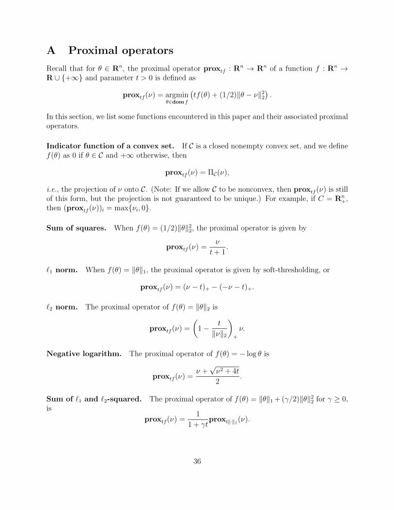
A Proximal operators

Recall that for θ ∈ Rn, the proximal operator proxtf : Rn → Rn of a function f : Rn →R ∪ {+∞} and parameter t > 0 is defined as

proxtf (ν) = argminθ∈dom f

(tf(θ) + (1/2)‖θ − ν‖22

).

In this section, we list some functions encountered in this paper and their associated proximaloperators.

Indicator function of a convex set. If C is a closed nonempty convex set, and we definef(θ) as 0 if θ ∈ C and +∞ otherwise, then

proxtf (ν) = ΠC(ν),

i.e., the projection of ν onto C. (Note: If we allow C to be nonconvex, then proxtf (ν) is stillof this form, but the projection is not guaranteed to be unique.) For example, if C = Rn

+,then (proxtf (ν))i = max{νi, 0}.

Sum of squares. When f(θ) = (1/2)‖θ‖22, the proximal operator is given by

proxtf (ν) =ν

t+ 1.

`1 norm. When f(θ) = ‖θ‖1, the proximal operator is given by soft-thresholding, or

proxtf (ν) = (ν − t)+ − (−ν − t)+.

`2 norm. The proximal operator of f(θ) = ‖θ‖2 is

proxtf (ν) =

(1− t

‖ν‖2

)+

ν.

Negative logarithm. The proximal operator of f(θ) = − log θ is

proxtf (ν) =ν +√ν2 + 4t

2.

Sum of `1 and `2-squared. The proximal operator of f(θ) = ‖θ‖1 + (γ/2)‖θ‖22 for γ ≥ 0,is

proxtf (ν) =1

1 + γtproxt‖·‖1(ν).

36

Quadratic. If f(θ) = (1/2)θTAθ + bT θ + c, with A ∈ Sn+, b ∈ Rn, and c ∈ R, then

proxtf (ν) = (I + tA)−1(ν − tb).If, e.g., f(θ) = 1

2‖Aθ − b‖22, then proxtf (ν) = (I + tATA)−1(ν − tAT b).

Poisson negative log likelihood. Here f(θ) =∑N

i=1 θ − yi log θ, where yi ∈ Z+ and

θ > 0. If we let S =∑N

i=1 yi, then

proxtf (ν) =ν − tN +

√(tN − ν)2 + 4tS

2.

Covariance maximum likelihood. Here

f(θ) = Tr(Sθ)− log det(θ).

We want to find proxtf (V ) := argminθ

(Tr(Sθ)− log det(θ) + (1/2t)‖θ − V ‖2F ). The first-

order optimality condition (along with the implicit constraint that θ � 0) is that the gradientshould vanish, i.e.,

S − θ−1 + (1/t)(θ − V ) = 0.

Rewriting, this is(1/t)θ − θ−1 = (1/t)V − S,

implying that θ and S− (1/t)V share the same eigenvectors [87], stored in Q. Let wi denotethe ith eigenvalue of θ, and si the ith eigenvalue of S − (1/t)V . Then we have

1/wi + (1/t)wi = si, i = 1, . . . , n.

To solve for w = (w1, . . . , wn), we solve these n 1-dimensional quadratic equations, with theith equation solved by

wi =tsi +

√t2s2i + 4t

2.

The proximal operator is then

proxtf (V ) = Qdiag(w)QT .

Bernoulli negative log-likelihood. Here

f(θ) = −(1Ty) log(θ)− (n− 1Ty) log(1− θ),with y ∈ Rn is problem data and θ ∈ [0, 1]. We want to find

proxtf (ν) := argminθ

(−(1Ty) log(θ)− (n− 1Ty) log(1− θ) + (1/2t)(θ − ν)2

).

By setting the derivative of the above argument with respect to θ to zero, we find that

θ3 − θ2(1− ν)− θ(nt− ν) + t1Ty = 0.

Solving this cubic equation (with respect to θ) for the solution that lies in [0, 1] yields theresult of the proximal operator.

37