A detailed workforce planning model including non- linear ...

A detailed workforce planning model including non-linear dependence of capacity on the size of the staff and cash management

Albert Corominas, Amaia Lusa, Jordi Olivella. EOLI – Enginyeria d’Organització i Logística Industrial IOC-DT-P-2010-01 Gener 2010

1

A detailed workforce planning model including non-linear dependence of capacity on the size of the staff and cash management

Albert Corominas, Amaia Lusa, Jordi Olivella

IOC Research Institute-Management Department, Universitat Politècnica de Catalunya, Barcelona, Spain

Avda. Diagonal 647, 11th floor, 08028 Barcelona, Spain. Tel. (+34) 934011705. Fax. (+34) 934016605. E-mail: [email protected]; [email protected]; [email protected]

Corresponding author: Amaia Lusa ([email protected])

Abstract

This paper introduces an original planning model which integrates production, human resources and cash management decisions, taking into account the consequences that decisions in one area may have on other areas and allowing all these areas to be coordinated. The most relevant characteristics of the planning problem are: (1) production capacity is a non-linear function of the size of the staff; (2) firing costs may depend on the worker who is fired; (3) working time is managed under a working time account (WTA) scheme, so positive balances must be paid to workers who leave the company; (4) there is a learning period for hired workers; and (5) cash management is included. A mixed integer linear program is designed to solve the problem. Despite the size and complexity of the model, it can be solved in a reasonable time. A numerical example is included to illustrate its performance.

Keywords: Production, aggregate planning, OR in manpower planning, mixed integer linear programming, working time accounts

1. Introduction

Aggregate planning (AP) deals with the problem of determining production inventory and workforce levels to cope with demand over a planning horizon that typically ranges from six months to one year. In classical approaches, the planning horizon is divided into one-month periods; demand, production and workforce are highly aggregated to reduce the size of the problem; cash management is not considered; and production is assumed to be linearly dependent on the volume of work. We propose a model that overcomes these limitations by simultaneously taking into account detailed planning of variations in staff numbers, non-linear dependence of capacity on the size of the staff and cash management.

2

AP models were first proposed by Holt et al. (1955). In their seminal work, the production and workforce levels are determined by minimising the cost of hiring, layoff, overtime, inventories and shortages. The cost functions are quadratic and the solution is obtained by means of a recursive procedure. Usually, the AP models generated are very computationally demanding and, until recently, only highly aggregated optimal plans could be solved. Although complex approximation techniques have been proposed, such as genetic algorithms (Fahimnia et al., 2006) and tabu search (Baykasoglu, 2001), computational difficulties have severely limited the adaptation of AP optimisation by companies. However, AP problems and other optimisation approaches can now be solved using conventional hardware and software. Consequently, optimisation tools have been used in combination with enterprise resource planning (ERP) systems to obtain optimal plans (Voß and Woodruff, 2005). In fact, optimisation is the basis of much of the newest planning software that is sold as modules or add-ons for ERP systems (Voß and Woodruff, 2006).

With the present computational capacity, it is possible to solve AP problems that include detailed information. Thus, AP becomes a more useful option, as we can: (1) work with shorter periods, typically weeks instead of months; (2) include more options in the models to be defined; (3) employ less aggregated data for both products and resources; (4) consider non-linear relations between factors; (5) adopt a stochastic approach; and (6) simultaneously take into account factors that were usually solved at different levels of the hierarchal models. A more detailed AP can be used to integrate the decisions of different company areas. As more factors can be included in the planning, more integrated decisions can be taken, and thus better solutions are found. Specifically, aspects such as worker’s shifts and cash management can be included. The integration of decisions is a current trend in planning (Singhal and Singhal, 2007).

Even though computational capacity has increased, it is far from unlimited. In addition, detailed information is not always available. Thus, the challenge is to define which areas the basic AP models need to be extended into and to devise a suitable new model. The literature shows several examples of this line of work. The model of Bhatnagar et al. (2007) includes sub-processes, workers’ skills, overtime and the number of contingent workers hired; that of Kanyalkar and Adil addresses (2005), long-term, medium-term and short-term plans simultaneously; and Venkateswaran and Son (2005) developed a multi-product, multi-facility, two-level model.

The contribution of the model that we propose in this paper is, first, to include a detailed plan of staffing needs. In the area of workforce planning, traditional AP models consider hiring, firing and overtime. We also consider the possibility of using working time accounts (WTAs). WTAs, like the annualisation of hours, are a system that provides flexibility in the hours worked by fixed staff, with no overtime

3

payments. In the WTA system, each worker has an account of working hours. The hours that he/she works above or below a standard value are credited or debited, respectively, to this account. This tool increases flexibility for the employee and the employer, as considered here. Planning with annualisation and WTA has been addressed previously (see, for example, Hung 1999, Corominas et al., 2002, Corominas et al., 2004, Azmat and Widmer 2004, Lusa et al. 2009). Our contribution here is to consider hiring, firing, overtime and WTAs together and to include all these possibilities in a detailed aggregate planning model.

A second contribution of this paper lies in the consideration of productivity functions that can be non-linear. AP models usually do not define a productivity function explicitly but use the expected worker productivity, which is assumed to be constant. This assumption implies that available hours of work and production capacity are proportionally related. We think that this is a limitation that has to be overcome, as stated by Pan and Kleiner (1995). A linear relation between resources and production generally cannot be assumed.

In fact, a linear relation between work and production can be a very unrealistic assumption, as proved by the literature. Ashcroft’s model (Ashcroft, 1950) implied that there was a non-linear relation between hours of work and production. It showed that, when the work consists in solving incidents in an automatic process, the contribution of each new worker will be lower because a new worker will only be useful when several failures happen simultaneously. On an assembly line, adding a new worker does not necessarily lead to a proportional increase in the output, as shown by Powell and Schmenner (2002). Organisational issues have been found to produce a non-linear relation between the number of members of a team and their outcomes (Tohidi and Tarokh, 2006).

Finally, the third element to outline as an original contribution of this paper is the inclusion in the model of detailed cash management prediction. Production planning that does not consider cash management can lead to unfavourable situations in terms of cost, and even to liquidity needs that cannot be attained by the company. The financial implications of decisions on production, inventory, hiring and firing are included in the proposed model. Less detailed AP models that include cash management are found in the literature (Kirca and Murat, 1996, Guillén et al., 2007).

After this Introduction, the paper is organized as follows: Section 2 describes the planning problem that is dealt with and Section 3 includes the optimisation planning model, which is a mixed integer linear program. In Section 4, the characteristics and the solution of an example are given to illustrate the performance of the model. In Section 5 the main results of a computational experiment are discussed. Finally, Section 6 contains the conclusions and the prospects of future research.

4

2. Problem description

The AP planning problem dealt with in this paper consists in determining, for each period of the planning horizon, the production of a set of products (or family of products) and their inventory levels, the number of workers belonging to the bottleneck section to be hired and/or dismissed and the number of hours that this section has to work, including the possibility of overtime and considering a WTA scheme.

When a worker is dismissed and his/her WTA balance is positive (he/she has worked more hours than the reference value), the company has to pay for these hours (in addition to severance pay and overtime).

The production capacity is assumed to depend on the number of working hours (which has to be determined) and on the number of workers (also to be determined), considering that non-experienced workers count less than fully experienced workers, depending on the number of worked periods (the learning effect is considered). Furthermore, the relation between the number of workers and the hourly capacity is assumed to be non-linear.

Cash management is also included in the planning problem. On the one hand, the cash inflow and outflow corresponding to a given period are collected and paid, respectively, after a given number of periods. On the other hand, the company is assumed to work with a credit account (with an available amount for credit purposes). The company has to pay for the borrowed amount and also for the available and non-borrowed amount. The balance of the credit account can also be positive, which generates a profit for the company.

The characteristics of the AP problem are summarized below:

There is a set of products (or families of products) whose demand (or a forecast of it) is known.

The products can be stored, and an inventory cost has to be considered. The warehouse has a finite capacity.

Production capacity depends on the capacity of a bottleneck section. Thus, only this section is considered in the planning of hiring/firing and working hours.

The capacity/hour of the bottleneck section depends non-linearly on the effective staff.

5

The effective staff is obtained by considering the number of fully experienced workers, which is equivalent to those workers whose seniority is equal to a given number of periods (a learning period is considered). For example, 10 workers, depending on the experience of each one of them, may be equivalent to 8.5 fully experienced workers.

A working time account scheme is considered, with the following characteristics:

There is a minimum and maximum number of working hours for each period. Above this maximum, hours are considered and paid as overtime (which is limited).

The WTA balance can be positive (the company owes hours to the worker), zero or negative (the worker owes hours to the company). There is a lower and an upper bound for the WTA balance.

The number of hours below/above the reference number is credited/debited to the WTA account, unless they are considered underaccount/overaccount hours. Underaccount/overaccount hours are those worked below/above the reference value that, instead of being credited/debited to the WTA account, are forgiven/paid to the worker (this is a common measure that it is used to allow an employee to work less/more hours when he/she has reached the lower/upper bound of the WTA balance).

The WTA balance of each available worker at the beginning of the planning horizon is known.

Hiring and firing is allowed during certain periods. Administrative costs are considered.

When a worker is dismissed, the company has to pay him/her severance pay, overtime and, if his/her WTA balance is positive, the hours of the WTA balance.

Cash inflow/outflow occurs a certain number of periods after the income/cost.

Cash flows are operated under a credit account. There are three different interest rates that apply, respectively, to the borrowed amount, the deposited amount and the available credit that is not used.

6

3. Planning model

The AP problem is formulated as a mixed integer linear program. The notation, the model and a description of the constraints are given below.

Data:

T Number of periods in the planning horizon (t=1,...,T).

0 Number of periods between a sale (output) and the corresponding cashing (an

invoice issued at t is cashed at t+0).

i Number of periods between the use of the resources (inputs) corresponding to

the variable costs and their payment (the resources used at t are paid at t+i).

P Number of periods in which the firm will pay salaries to the workers. P is also the number of periods in which the firm can hire workers.

pj Periods in which the firm will pay salaries to the workers (j=1,...,P), where

1; 1,..., 1p pj j j P . For the sake of simplicity, we assume p

P T .

Dismissals can happen only at the end of pj periods (j=1,...,P-1). Retirement

and forecast resignations can occur at the end of pj (j=1,...,P). However,

retirement and resignations that take place at the end of period T are irrelevant for planning purposes.

hj Periods at the beginning of which the firm can hire workers (j=1,...,P), where

1 1h and 1 1h pj j (j=1,...,P-1).

B Maximum amount of the absolute value of a negative balance on the rewarded credit account.

, ,b d a bt t t ti i i i Rates of interest that apply, respectively, to the borrowed amount (the

absolute value of the balance of the account, when it is negative), to the deposited amount (the balance of the account, when it is positive) and to the credit that is available and not used (B minus the absolute value of the negative balance of the account). We assume that interest is credited or debited to the account during the periods in which it is earned or due (t=1,...,T).

0b Initial balance of the credit account (which, of course, may be positive, null or

negative, provided that it is B ).

7

tBF Balance of cashing and payments that are fixed before the beginning of the

planning horizon (i.e. they do not depend on the decisions involved in the model), corresponding to period t (t=1,...,T). The balance may have positive (when cashing is greater than payments), null or negative values.

N Number of products (or families of products) (n=1,...,N).

ntd Demand for product n in period t (n=1,...,N; t=1,...,T).

0ns Initial inventory of product n (n=1,...,N).

Tns Desired inventory of product n (n=1,...,N) at the end of the planning horizon.

n Units of capacity of the warehouse that are required to store a unit of product n

(n=1,...,N).

WQ Capacity of the warehouse.

ntp Sale price of product n in period t (n=1,...,N; t=1,...,T).

ntpc Variable cost of producing a unit of product n in period t, excluding the cost of

the staff (n=1,...,N; t=1,...,T).

ntwc Variable cost of storing a unit of product n in period t (excluding the cost of

the staff) (n=1,...,N; t=1,...,T-1).

n Coefficient used to penalize lost demand of product n (n=1,...,N).

0W Number of workers in the bottleneck section at the beginning of the planning

horizon (old workers).

0W Number of old workers in the bottleneck section whose retirement or

resignation is forecast within the planning horizon. These workers are

assumed to be 0ˆ1,...,i W . Workers 0 0

ˆ 1,...,i W W will not leave the firm

during the planning horizon unless they are dismissed.

iJ An integer value in 1,..., P . Old worker i 0ˆ( 1,..., )i W will retire or resign at

the end of period i

pJ .

8

j Number of fully experienced workers equivalent to a worker whose seniority

is equal to j-1 periods (j=1,...,T), where

11 ( 1,..., ), ( 1,..., 1)j j jj T j T .

swi Seniority of worker i at the beginning of the planning horizon (i=1,...,W0).

0tw Number of old workers at the beginning of period t (t=1,...,T), taking into

account those workers whose retirement or resignation is forecast within the planning horizon (the real number of workers may vary because of hiring and firing).

H Upper bound on the number of workers hired in a period (new workers).

,t tLW UW Lower and upper bounds on the total number of workers in period t

(t=1,…,T).

B kQ w Hourly capacity of the bottleneck section, which monotonically depends on

the effective size of the staff of the section (see below), defined for np values kw (k=1,...,np), where 1k kw w (k=1,...,np-1). Note that 1w and npw are,

respectively, a lower and an upper bound on the value of the effective size of

the staff of the bottleneck section, and therefore 1BQ w and B npQ w are,

respectively, lower and upper bounds of the hourly capacity of the bottleneck section.

n Units of capacity of the bottleneck section required to obtain a unit of product

n (n=1,...,N).

HC Administrative costs of hiring a worker.

DC Administrative costs of dismissing a worker.

itcl Cost of labour, at period t (t=1,…,T), corresponding to old worker i

0( 1,..., )i W .

tcln Cost of labour, at period t (t=1,…,T), for each new worker.

0isp Severance pay of old worker i if he/she was dismissed at the beginning of the

planning horizon 0 0ˆ( 1,..., )i W W .

9

ispp Severance pay per each worked period in the planning horizon, corresponding

to old worker i 0 0ˆ( 1,..., )i W W .

0spp Severance pay per each worked period in the planning horizon, corresponding

to a new worker.

0, , ,h h h h Minimum number, reference number, maximum number (excluding

overtime) and maximum number (including overtime) of working hours (all of

them per period), respectively (where 0h h h h ). The difference

between the worked hours in [ ,h h ] and h is debited or credited to the WTA,

according to its sign. Hours above h and up to h are paid as overtime.

,A A Upper bounds on the absolute value of the negative balance and the positive

balance, respectively, of the working time accounts.

,T TA A Upper bounds on the absolute value of the negative balance and the positive

balance, respectively, of the working time accounts at the end of the planning horizon.

O Upper bound on the overaccount hours.

0iwa Balance of the WTA of old worker i at the beginning of the planning horizon.

V Maximum number of hours of overtime for the whole planning horizon.

covti Cost of an hour of overtime corresponding to old worker i (i=1,...,W0).

covt0 Cost of an hour of overtime corresponding to a new worker.

covaci Cost of an overaccount hour corresponding to old worker i (i=1,...,W0).

covac0 Cost of an overaccount hour corresponding to a new worker.

cbi Amount to be paid to old worker i (i=1,...,W0), for each hour of the positive balance of her/his WTA, if the worker leaves the firm or is dismissed.

cb0 Amount to be paid to a new worker for each hour of the positive balance of her/his WTA in the case of dismissal.

10

Variables:

tQ Capacity of the bottleneck section in period t (t=1,...,T).

ntq Number of units of product n manufactured in period t (n=1,...,N;

t=1,...,T).

nts Inventory of product n at the end of period t (n=1,...,N; t=1,...,T-1).

ntr Lost demand of product n in period t (n=1,...,N; t=1,...,T).

,t tb b Absolute values of the non-positive and non-negative balances,

respectively, of the credit account at the end of period t (t=1,...,T).

tw Effective size of the staff at the beginning of period t (t=1,...,T).

ikdow 0,1 Binary variable equal to 1 iff old worker i is dismissed at the end of

period pk 0 0

ˆ( 1,..., ; 1,..., 1)i W W k P .

jnw Number of workers hired at the beginning of period hj (j=1,...,P).

jkdnw Number of workers dismissed at the end of period pk (k=j,...,P-1) out

of those hired at the beginning of period hj (j=1,...,P-1).

th Number of working hours in t, excluding overtime (t=1,...,T).

tv Number of hours of overtime in t (t=1,...,T).

ikpovto Payment for overtime corresponding to old worker i at the end of

period pk 0

ˆ( 1,..., ; 1,..., )i W W k P . These variables do not need to

be defined for workers 0ˆ1,...,W because this payment can be directly

obtained by multiplying the overtime cost by the number of overtime hours (for the other workers, it has to be considered whether they have been dismissed or not; see Equation 14).

jkpovtn Payment for overtime corresponding to workers hired at the beginning

of period hj (j=1,...,P) and not dismissed before the end of period p

k

(k=j,...,P).

11

ikpovaco Payment for overaccount hours corresponding to old worker i at the

end of period pk 0

ˆ( 1,..., ; 1,..., )i W W k P . These variables do not

need to be defined for workers 0ˆ1,...,W because this payment can be

directly obtained by multiplying the overaccount cost by the number of overaccount hours (for the other workers, it has to be considered whether they have been dismissed or not; see Equation 16).

jkpovacn Payment for overaccount hours corresponding to workers hired at the

beginning of period hj (j=1,...,P) and not dismissed before the end of

period pk (k=j,...,P).

,it itwao wao Non-negative and non-positive parts of the balance of the WTA

of old worker i at the end of period t

0 0 0ˆ ˆ( 1,..., ; 1,..., ; 1,..., ; 1,..., )

i

pJi W t i W W t T .

,jt jtwan wan Non-negative and non-positive parts of the balance of the

working time accounts, at the end of period t, for the workers hired athj ( 1,..., ; ,..., )h

jj P t T .

ito , ito Number of overaccount and underaccount hours, respectively,

corresponding at period t to worker i, who belongs to the initial staff

0 0 0ˆ ˆ( 1,..., ; 1,..., ; 1,..., ; 1,..., )

i

pJi W t i W W t T .

jtn , jtn Number of overaccount and underaccount hours, respectively,

corresponding at period t to each worker hired at hj

( 1,..., ; ,..., )hjj P t T .

ijpdwao Amount to be paid, due to a positive balance on the working time

account, to old worker i if he/she is dismissed at the end of period pk

0 0ˆ( 1,..., ; 1,..., 1)i W W j P . These variables do not need to be

defined for workers 0ˆ1,...,W because this payment can be directly

obtained by multiplying the cost of an hour of positive balance by the positive balance during the period in which they leave the company (for the other workers, it has to be considered whether they have been dismissed or not; see Equation 18).

12

jkpdwan Aggregate amount to be paid, due to a positive balance on their

working time accounts, to workers hired at hj and dismissed at the end

of period pk (j=1,...,P-1; k=j,...,P-1).

ivwao Monetary value of the balance on the working time account of old

worker i at the end of the planning horizon 0 0ˆ( 1,..., )i W W .

jvwan Monetary value of the balance on the working time accounts at the end

of the planning horizon for the workers hired at hj (j=1,...,P).

Qkt 0,1 Auxiliary binary variables to linearise the total capacity of a period, i.e.

the product of the hourly capacity by the number of working hours

(k=1,...,np; t=1,...,T); 1Qkt if the hourly capacity at period t is equal to

B kQ w .

Djkn 0,1 Auxiliary binary variables to linearise payments corresponding to the

dismissal of new workers (j=1,...,P-1; k=j,...,P-1; n=0,...,H); 1Djkn iff

the number of workers hired at hj and dismissed at the end of period

pk is equal to n.

Hjkn 0,1 Auxiliary binary variables to linearise payments corresponding to

workers hired in the planning horizon (j=1,...,P; k=j,...,P; n=0,...,H);

1Hjkn if the number of workers hired at h

j who remain in the firm at

the end of period pk is equal to n.

jn 0,1 Auxiliary binary variables (j=1,...,P; n=0,...,H); 1jn iff the number

of workers hired at hj is equal to n.

13

Model:

0

0

0 1

1

1 1 1 1

1

ˆ 1 1 1 1i= +1

ˆ

1 1 1

max · · ·

· ·

· 1

p ppJi k

h hk

T N T Td b a

nt nt nt t t t t tt n t t

W P T N T N

i j nt nt nt ntj=1 t n t nW

WPH

j it it itj i t t t

z p d r i b i i b

vwao vwan pc q wc s

C nw cl cl cl dow

0

0

0

0 0

1

ˆ 2 11

1 1

1 1 1

ˆ ˆ 11 | 1

·

p pj k

h hj k

pk

hi k

W P k

ijk ji W

P P P k

j t t j jlj j k j l jt t

W k

i t ik jkji W J k i Wt

nw cln cln nw dnw

covt v povto povtn

0

0 0

0 0

0 0

1

ˆ ˆ1 11 | 1

1 1 1 10

ˆ ˆ1 1 11 1

0

·

· · ·

·

pk

hi k

P

k

WP k

i it ik jkk ji W J k i Wt

W WP P P PD p

ij jk i i j ijj j k j ji W i W

pk j

covac o povaco povacn

C dow dnw sp spp dow

spp

0 0

0

ˆ1 1 1

,ˆ1 1 11

1 1

1 t=1 1

1 · pJi

W WP P Ph

jk i ijij k j i ji W

P P T N

jk n ntj k j n

dnw cb wao pdwao

pdwan r

(1)

subject to

1

1,..., 1P

jk jk j

dnw nw j P

(2)

00ˆˆ 1[1,..., ]| [1,..., 1] |

1[1,..., ] | [ ,..., ] |

1

· 1,...

0

i ip p

kJi

hjh p

j k

W

t ws t ws t iki Wi W t k P t

j jktj P t k j P t

w dow

nw dnw t

,T

(3)

0

0

ˆ 1 [1,..., ] | [1,..., ] | [ ,..., ] |

1,...,0

p h pjk k

W

t t ik j jk ti W j P tk P t k j P t

LW w dow nw dnw UW t T

(4)

14

1

1

1

· 1,...,

1 1,...,

· · · · 1

1,..., ; 1,...,

npk Q

t ktk

np

ktk

B k B np B Qt t t kt

w w t T

t T

Q Q w h v Q w h Q w h

t T k np

(5)

1

· 1,...,N

n nt tn

q Q t T

(6)

01 1 1 1

, 1

, 1

1,...,

1,..., ; 2,..., 1

1,...,

n n n n n

nt n t nt nt nt

Tn n T nT nT nT

s s q d r n N

s s q d r n N t T

s s q d r n N

(7)

1

· 2,..., 1N

Wn nt

n

s Q t T

(8)

0 01 1 1 1 1 0

0, 1 , 1

0

0, 1 , 1

1 0 0

0

1,...,

ˆ2,..., ; 1,...,

ˆ2,..., ; 1,...,

i

i i i i i

it it i t i t t it it

pJ

it it i t i t t it it

p

wao wao wa h h o o i W

wao wao wao wao h h o o

t i W

wao wao wao wao h h o o

t i W W

h

, 1[1,..., 1] |

0, 1

[1,..., 1] |

2 0 0

'

ˆ,..., ; 1,...,

pk

pk

ik it it i tk P t

i t t it it ikk P t

h

M dow wao wao wao

wao h o o h M dow

t T i W W

(9)

15

0

0, 1 , 1

0, 1,0

1,...,

1,..., ; 1,...,

h h h h hj j j j jj j j j

jt jt j t j t t jt jt

h pj j

j k

wan wan h h n n

j P

wan wan wan wan h h n n

j P t

h M

0, 1 , 1 , 1,0

2,..., ; 1,..., ; ...,

H Hjt jt j t j t t jt jt j k

h pk k

wan wan wan wan h n n h M

j P k j P t

(10)

1

T

tt

v V

(11)

1

0 01

ˆ1 1,...,P

ikk

dow i W W

(12)

1

0

·

1,...,

1

H

j jnn

H

jnn

nw n

j P

(13)

1

0

·

1,..., ; ,...,

1

k HH

j jl jknl j n

HHjkn

n

nw dnw n

j P k j P

(14)

1

1

0 0

· ·min , 1 . ·

ˆ 1,..., ; 1,...,

pj

hj

jp h

ik i t i j j ikkt

povto covt v covt V h h dow

i W W j P

(15)

0 0

0 0 , 1,

· · ·min , 1 . · 1

1,..., ; 1,...,

· · ·min , 1 . · 1

1,..., ; 1,..., ; 1,...,

pj

hj

pk

hk

p hjj t j j jn

t

p h Hjk t k k j k n

t

povtn n covt v covt V h h

j P n H

povtn n covt v covt V h h

j P k j P n H

(16)

16

1

0

1

0 0

· · 1 . ·

ˆ 1,..., ; 1,...,

pk

hk

kp h

ik i it i k k ijjt

povaco covac o covac h h dow

i W W k P

(17)

00 0

00 0 , 1,

· · · 1 . · 1

1,..., ; 1,...,

· · · 1 . · 1

1,..., ; 1,... ; 1,...,

pj

hj

pk

hk

p hjj jt j j jn

t

p h Hjk jt k k j k n

t

povacn n covac n covac h h

j P n H

povacn n covac n covac h h

j P k j P n H

(18)

,

0 0

· · 1

ˆ 1,..., ; 1,..., 1

pj

ij i i ijipdwao cb wao cb A dow

i W W j P

(19)

1

0

0 0

·

1 1,..., 1; ,..., 1

· · · · · 1

0,...,

pk

HD

jk jknn

HDjkn

n

Djk jknj

dnw n

j P k j P

pdwan cb n wan cb H A

n H

(20)

1

1

1

1

1 1

1 1

0 0

· · · ;

· · ·

· · 1 ; · · 1

ˆ 1,...,

P

i i iT iT i ijj

P

i i iT iT i ijj

P P

i i ij i i ijj j

vwao cb wao wao cb A dow

vwao cb wao wao cb A dow

vwao cb A dow vwao cb A dow

i W W

(21)

0 0

0 0

· · · · · 1

· · · · · 1

1,..., 1; ,..., 1; 0,...,

p pk k

p pk k

Hj jPnj j

Hj jPnj j

vwan cb n wan wan cb H A

vwan cb n wan wan cb H A

j P k j P n H

(22)

17

0

0

1 1

, , , , , , ,1 1 1

ˆ ' 1

' 'ˆ 111|

· 1 · 1 ·

· · · ·

1

o o o i i i i

pJi

d b a at t t t t t t t t

N N NH

kn t n t n t n t n t n t n tn n n

W k

ik ik ijji Wi t

b b b i b i i B i BF

p d r pc q wc s C nw

cl cl dow

0

' 0

0 0 0'

0

0

'

'|

' 'ˆ ˆ ˆ'1 | ' 1 1 | '

'ˆ 1

·

· ·

hj

p pk k

h hi ik k

W k

k j jll jj t

W

i t ik jk i itj ki W J k i W i W J kt t

W

ik jkj ki W

D

cln nw dnw

covt v povto povtn covac o

povaco povacn

C

0 0

0 0

0

'0 0

0' ' ' ' 0 ' '

ˆ ˆ1 1| |

' ',ˆ ˆ '1 | ' 1

· · · · 1 ·

1,...,

h hj j

pk

i

W Wp p h

ik jk i i k ik k j jki W i Wj t j t

W

i ik jkij ki W J k i W

dow dnw sp spp dow spp dnw

cb wao pdwao pdwan

t T

(23)

0

0 0

1,...,

0 1,...,

1,...,

ˆ; 1,..., ; 1,..., |

ˆ; 1,..., ; 1,..., 1

; 1,..., ; ,..., 1

;

i

t

t

j

pit it J

it it

hjt jt j

iT T i

h h h t T

v h h t T

nw H j P

wao A wao A i W t t T

wao A wao A i W W t T

wan A wan A j P t T

wao A wao

0

0 0 0

1,...,

; 1,...,

ˆ ˆ 1,..., ; 1,..., ; 1,..., ; 1,...,

1,..., ; ,...,

1,...,

i

T T

jT T jT T

pit J

hjt j

t

A i W

wan A wan A j P

o O i W t i W W t T

n O j P t T

b B t T

(24)

The objective function (1) includes the income and the costs that depend on planning decisions: income from the demand that is met and from the positive balance in the credit account, variable costs of production and warehousing, administrative costs of hiring workers, cost of labour of old and new workers, cost of overtime and of overaccount hours, administrative costs of dismissing workers, severance pay, payments corresponding to positive balances on the working time accounts of dismissed workers, interest on the credit account, and finally the monetary value of

18

the balances of the WTAs of the workers who remain at the end of the planning horizon. It also includes a lost demand penalisation.

The meaning of the constraints is as follows: (2) the number of workers hired during a period is greater than or equal to the number of new workers that are dismissed, until the end of the planning horizon; (3) computes the effective size of the staff; (4) imposes the lower and the upper bound on the real number of workers; (5) fixes production capacity as a function of the effective size of the staff; (6) establishes the production capacity; (7) balances inventories; (8) sets the warehousing capacity.

Equations (9) and (10) establish the working time accounts of old and new workers, respectively (the WTA balance only applies when workers have not been dismissed); (11) sets the upper bound on overtime; (12) establishes that an old worker can be dismissed at most once; (13) and (14) establish the relation between the number of workers that remain in a period out of those hired during a preceding period, and the auxiliary binary variables that allow the linearisation of several payments and values corresponding to new workers; (15) and (16) model the payments for the overtime of old and new workers, respectively (only for non-dismissed workers); (17) and (18) model the payments for overaccount hours of old and new workers, respectively; (19) and (20) model payments corresponding to positive balances of the WTAs of old and new workers, respectively, in the case of dismissal; (21) and (22) correspond to the balances of WTAs of old and new workers, respectively, at the end of the planning horizon.

Equation (23) corresponds to the cash balance. Input and output varies depending on the period, generating a variety of forms for the constraints. In order to shorten the presentation, (23) incorporates all kinds of inputs and outputs on the right-hand side, which have been grouped into blocks and are placed between square brackets.

The first block is common to all periods in the planning horizon and includes the variation in the balance of the credit account, the interest, and the balance between cashing and payments that do not depend on the planning decisions. The second block

(sales) is present only in periods when ot . The third one (variable costs of

production and storage), in periods when it . The fourth block corresponds to the

administrative costs of hiring workers and is present only when | hkk t . The fifth

block corresponds to the payroll of old workers and of workers hired during the planning horizon, as well as payments for overtime and overaccount hours corresponding to old workers. The sixth block represents the payments due to dismissals (or workers who leave the company). Therefore, these last two blocks shall

be present only when '' | pkk t . Of course, for 1t the left-hand side is equal to 0b .

Finally, (24) sets lower and upper bounds on several variables.

19

4. Numerical example

To illustrate the performance of the model, the results of an example are given below. The data used for the experiment are given in Table 1.

Table 1. Data for the example

T 52 weeks

0,

i 8, 8 weeks

pj ,

hj

periods {4, 8, 12, 16, 20, 24, 28, 32, 36, 40, 44, 48, 52}, {1, 5, 9, 13, 17, 21, 25, 29, 33, 37, 41, 45, 49}

B 150,000 monetary units

, ,b d a bt t t ti i i i 0.0015, 0.0004, 0.0006

0b 20,000 monetary units

tBF -4,000 monetary units

N 1 product family

ntd A seasonal demand has been generated (see Figure 2) 0ns ,

Tns 300, 300 product units

WQ 1,500 product units

ntp 22 monetary units

ntpc 10% of pnt monetary units

ntwc 0.05·pnt monetary units

n 0

0W , 0W , iJ There are 8 workers at the beginning of the planning horizon; 2 of these workers will retire in periods 16 and 36, respectively.

j {0.5, 0.55, 0.6, 0.65, 0.7, 0.75, 0.8, 0.85, 0.9, 0.95, 1, ..., 1} workers

swi 1 (initial workers are assumed to be fully experienced).

0tw {8,8,8,8,8,8,8,8,8,8,8,8,8,8,8,8,7,7,7,7,7,7,7,7,7,7,7,7,7,7,7,7,7,7,7,7,6,6,6,6

,6,6,6,6,6,6,6,6,6,6,6,6} workers

H 10 workers

,t tLW UW 5, 20 workers

B kQ w See Figure 1

n 0.5 hours/unit

HC , DC 150, 200 monetary units /worker

itcl , tcln {600, 600, 420, 420, 450, 500, 500, 550}, 400 monetary units /period-worker

0isp , ispp {1800, 1800, 3600, 5400, 5400, 7200} monetary units, {35, 35, 40, 45, 45,

50} monetary units /period

0spp 50 monetary units /period-worker 0, , ,h h h h 24, 40, 45, 48 hours

[ , ],[ , ]T TA A A A [150, 150], [50, 50] hours

O 50 hours 0iwa {-15, -10, -5, 0, 5, 10, 15, 20} hours

20

V 80 hours

covti , covt0 50, 40 monetary units /hour

covaci, covac0 60, 50 monetary units /hour

cbi, cb0 50, 40 monetary units /hour

Figure 1. Non-linear capacity for the example

The example, which has 11,378 variables (5,597 of which are binary variables and 65 integer and non-binary) and 11,223 constraints, was solved using ILOG CPLEX 11.0, with a relative gap of 0.05%. Solving the model took over an hour (77 minutes on a Pentium IV at 3.0 GHz and 3 GB of RAM). However, considering the type of problem being solved, this is an acceptable solving time.

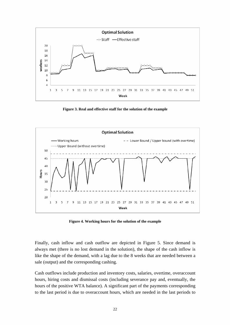
The demand, production and inventory are shown in Figure 2. Figure 3 includes the number of workers (staff) and the effective staff, which takes into account the fact that new workers need a learning period to be as efficient as fully experienced workers. Figure 4 shows the number of working hours.

Figure 2 shows that production is quite high during the first demand peak (otherwise demand could not be met). This high production level is possible because of the increase in capacity that is achieved when additional workers are hired (see Figure 3). When the low demand period starts, some workers are dismissed. This reduces the system’s production capacity. During this low demand period, production is higher than demand so inventory can be stored. This inventory allows the company to meet demand during the second demand peak without having to hire a large number of workers to increase the production capacity.

The workers that are hired to meet the first demand peak are dismissed when demand starts to diminish. To avoid paying a large number of hours from their WTA balance,

21

the number of working hours in the periods in which these workers are in the company have values that allow for flexibility to meet demand and make it possible to maintain the WTA balances close to 0, so money is saved when these workers are dismissed.

The possibility of hiring and dismissing workers and the use of a WTA system provide enough flexibility to meet demand optimally. An increase in capacity can be obtained by hiring workers and by increasing the number of working hours. Both options have costs (hiring and dismissal costs and the positive WTA balance cost when a worker is dismissed). Determining the best combination, for each period, after a consideration of all the problem constraints, would be a hard (and even impossible) task without an optimization planning model such as the one proposed in this paper.

Figure 2. Demand, production and inventory for the solution of the example

22

Figure 3. Real and effective staff for the solution of the example

Figure 4. Working hours for the solution of the example

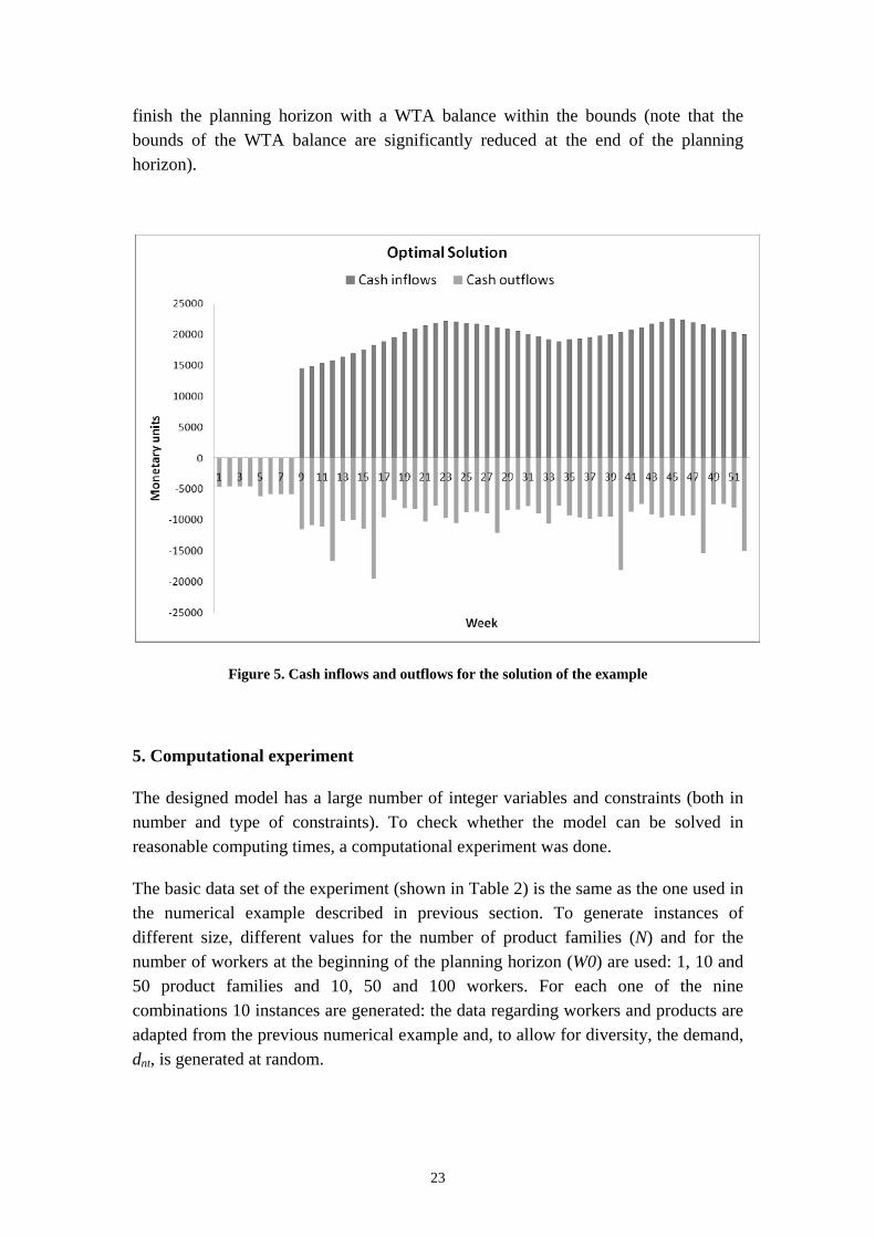
Finally, cash inflow and cash outflow are depicted in Figure 5. Since demand is always met (there is no lost demand in the solution), the shape of the cash inflow is like the shape of the demand, with a lag due to the 8 weeks that are needed between a sale (output) and the corresponding cashing.

Cash outflows include production and inventory costs, salaries, overtime, overaccount hours, hiring costs and dismissal costs (including severance pay and, eventually, the hours of the positive WTA balance). A significant part of the payments corresponding to the last period is due to overaccount hours, which are needed in the last periods to

23

finish the planning horizon with a WTA balance within the bounds (note that the bounds of the WTA balance are significantly reduced at the end of the planning horizon).

Figure 5. Cash inflows and outflows for the solution of the example

5. Computational experiment

The designed model has a large number of integer variables and constraints (both in number and type of constraints). To check whether the model can be solved in reasonable computing times, a computational experiment was done.

The basic data set of the experiment (shown in Table 2) is the same as the one used in the numerical example described in previous section. To generate instances of different size, different values for the number of product families (N) and for the number of workers at the beginning of the planning horizon (W0) are used: 1, 10 and 50 product families and 10, 50 and 100 workers. For each one of the nine combinations 10 instances are generated: the data regarding workers and products are adapted from the previous numerical example and, to allow for diversity, the demand, dnt, is generated at random.

24

The maximum computing time was set to 7,200 seconds (two hours), which is a short time considering the kind of problem being solved. Only one of the instances finished before the time limit. The results of the experiments are summarized in Table 3, where the number of variables, the number of constraints and the average value for the relative gap are shown. Overall, it can be concluded that the results are good enough.

Table 2. Data of the computational experiment

T 52 weeks

0,

i 8, 8 weeks

pj ,

hj

periods {4, 8, 12, 16, 20, 24, 28, 32, 36, 40, 44, 48, 52}, {1, 5, 9, 13, 17, 21, 25, 29, 33, 37, 41, 45, 49}

B 15,000* W0 monetary units

, ,b d a bt t t ti i i i 0.0015, 0.0004, 0.0006

0b 0 monetary units

tBF 0 monetary units

N 1 / 10 / 50 product families

ntd A random value between 0.95*min(QB)*40 and 1.05*max(QB)*40 is generated. The demand for each product, dnt, is obtained by dividing this value by N.

0ns ,

Tns 0, 0 product units

WQ 1.2*max(demt) product units

ntp 20 monetary units

ntpc 2 monetary units

ntwc 1 monetary units

n 0

0W , 0W , iJ W0: 10 / 50 / 100 workers

0ˆ 0, iW J

j {1, ..., 1} workers

swi 1, for all i (workers are supposed to be fully experienced)

0tw W0 workers, for all t

H 5, 15 and 25 workers for W0 equal to 10, 50 and 100, respectively

,t tLW UW (4, 20), (20,100) and (30, 200) workers for W0 equal to 10, 50 and 100 workers, respectively

B kQ w Adapted from the example, with wk ranging from [4-20], [20-100] and [30-200] for W0 equal to 10, 50 and 100 workers, respectively

n 1 hours/unit

HC , DC 150, 200 monetary units/worker

itcl , tcln 500, 400 monetary units/period·worker

0isp , ispp 3500, 40 monetary units/period

0spp 50 monetary units/period·worker 0, , ,h h h h 24, 40, 45, 48 hours

25

[ , ],[ , ]T TA A A A

[150, 150], [50, 50] hours

O,

0iwa , V 50, 0 and 80 hours

covti , covt0 50, 40 monetary units/hour

covaci, covac0 60, 50 monetary units/hour

cbi, cb0 50, 40 monetary units/hour

Table 3. Results of the computational experiment

W0 10 50 100

N

1

Var.: 11,000 (4,694 binary) Constr.: 10,524 Gap: 0.19



10




50




6. Conclusions and future research

In this paper, we present a new planning model which integrates production, human resources (hiring and firing and working time planning) and cash management decisions. It overcomes the limitations of traditional planning models, which only consider production—and in some cases other areas—in a fairly simple way. The model allows the relations between the different areas to be considered, so that they can be coordinated optimally.

The most relevant characteristics of the planning problem are: the non-linear dependence of production capacity on the effective size of the staff; the dependence of firing costs on the specific worker who is fired and on the balance of his/her working time account (hence each worker must be considered individually, which increases the size of the model); the learning period for hired workers; and the cash management, which is included.

A detailed mixed integer linear program was designed to solve the problem. The model, which has a large number of variables (both real and integer) and constraints (both in number and type), can be solved in reasonable times with standard

26

optimization software. The performance of the model is illustrated by a numerical example and a computational experiment.

Our immediate research objectives for planning models are to include other kinds of decisions in the model. First, we want to consider supplies in a multi-supplier environment (considering different price, quality and lead time conditions for different suppliers); second, we wish to include marketing decisions in the model (decisions on the price of the products, the promotion investments, etc.); and finally, we wish to design planning models that integrate the most relevant areas of a company.

Acknowledgements

Paper supported by the Spanish Ministry of Science and Technology, project DPI2007-61588, and co-financed by the ERDF.

References

Ashcroft H. (1950). The Productivity of Several Machines Under the Care of One Operator. Journal of the Royal Statistical Society. Series B (Methodological), 12, 145-151.

Azmat C, Widmer M. (2004). A case study of single shift planning and scheduling under annualized hours: A simple three step approach. European Journal of Operational Research, 153, 148-175.

Baykasoglu A. (2001). MOAPPS 1.0: aggregate production planning using the multiple-objective tabu search. International Journal of Production Research, 39, 3685-3702.

Bhatnagar R, Saddikutti V, Rajgopalan A. (2007). Contingent manpower planning in a high clock speed industry. International Journal of Production Research, 45, 2051-2072.

Corominas A, Lusa A, Pastor R. (2002). Using MILP to plan annualised working hours. Journal of the Operational Research Society, 53, 1101-1108.

Corominas A, Lusa A, Pastor R. (2004). Planning annualised hours with a finite set of weekly working hours and joint holidays. Annals of Operations Research, 128, 217-233.

27

Corominas A, Lusa A, Pastor R. (2007). Using a MILP model to establish a framework for an annualised hours agreement. European Journal of Operational Research, 177, 1495-1506.

Fahimnia B, Luong LHS, Marian RM. (2006). Modeling and Optimization of Aggregate Production Planning-A Genetic Algorithm Approach. Proceedings of World Academy of Science, Engineering and Technology, 15.

Guillén G, Badell M, Puigjaner L. (2007). A holistic framework for short-term supply chain management integrating production and corporate financial planning. International Journal of Production Economics, 106, 288-306.

Holt CC, Modigliani F, Simon HA. (1955). A linear decision rule for production and employment scheduling. Management Science, 1-30.

Hung R. (1999). Scheduling a workforce under annualized hours, International Journal of Production Research, 37, 2419-2427.

Kanyalkar A P, Adil GK. (2005). An integrated aggregate and detailed planning in a multi-site production environment using linear programming. International Journal of Production Research, 43, 4431-4454.

Kirca Ö, Murat M. (1996). An integrated production and financial planning model and an application. IIE transactions, 28, 677-686.

Lusa A, Corominas A, Olivella J, Pastor R. (2009). Production planning under a working time accounts scheme. International Journal of Production Research, 47, 3435-3451.

Pan L, Kleiner BH. (1995). Aggregate planning today. Work Study, 44, 4–7.

Powell PT, Schmenner RW. (2002). Economics and operations management: towards a theory of endogenous production speed. Managerial and Decision Economics, 23.

Singhal J, Singhal K. (2007). Holt, Modigliani, Muth, and Simon's work and its role in the renaissance and evolution of operations management. Journal of Operations Management, 25, 300-309.

Tohidi H, Tarokh MJ. (2006). Productivity outcomes of teamwork as an effect of information technology and team size. International Journal of Production Economics, 103, 610-615.

Venkateswaran J, Son YJ. (2005). Hybrid system dynamic—discrete event simulation-based architecture for hierarchical production planning. International Journal of Production Research, 43, 4397-4429.

28

Voß S, Woodruff DL. (2005). Connecting MRP, MRP II and ERP — Supply Chain Production Planning Via Optimization Models. Tutorials on Emerging Methodologies and Applications in Operations Research.

Voß S, Woodruff DL. (2006). Introduction to Computational Optimization Models for Production Planning in a Supply Chain, Springer-Verlag New York, Inc. Secaucus, NJ, USA.

A detailed workforce planning model including non- linear ...

Documents

Transcript of A detailed workforce planning model including non- linear ...