A Design Methodology for Bus Transit Networks with...
199
TTS Southwest Region University Transportation Center , A Desi gn Methodology for B us Tra ns it Netw or ks wit h Coordinated Operations --_.- SWUTC/94/60016-1 Center for Transportation Research University of Texas at Austin 3208 Red River, Suite 200 Austin, Texas 78705-2650 -- -
Transcript of A Design Methodology for Bus Transit Networks with...

M~- bd-~
TTS Southwest Region University Transportation Center
,
A Design Methodology for Bus Transit Networks
with Coordinated Operations
~ ~-~-~-.-- --_.- -~-~-- ~ --- ~~ ~~-~
SWUTC/94/60016-1
Center for Transportation Research University of Texas at Austin
3208 Red River, Suite 200 Austin, Texas 78705-2650
.~~-~ -~- -- - - - ~.~--~-----------~
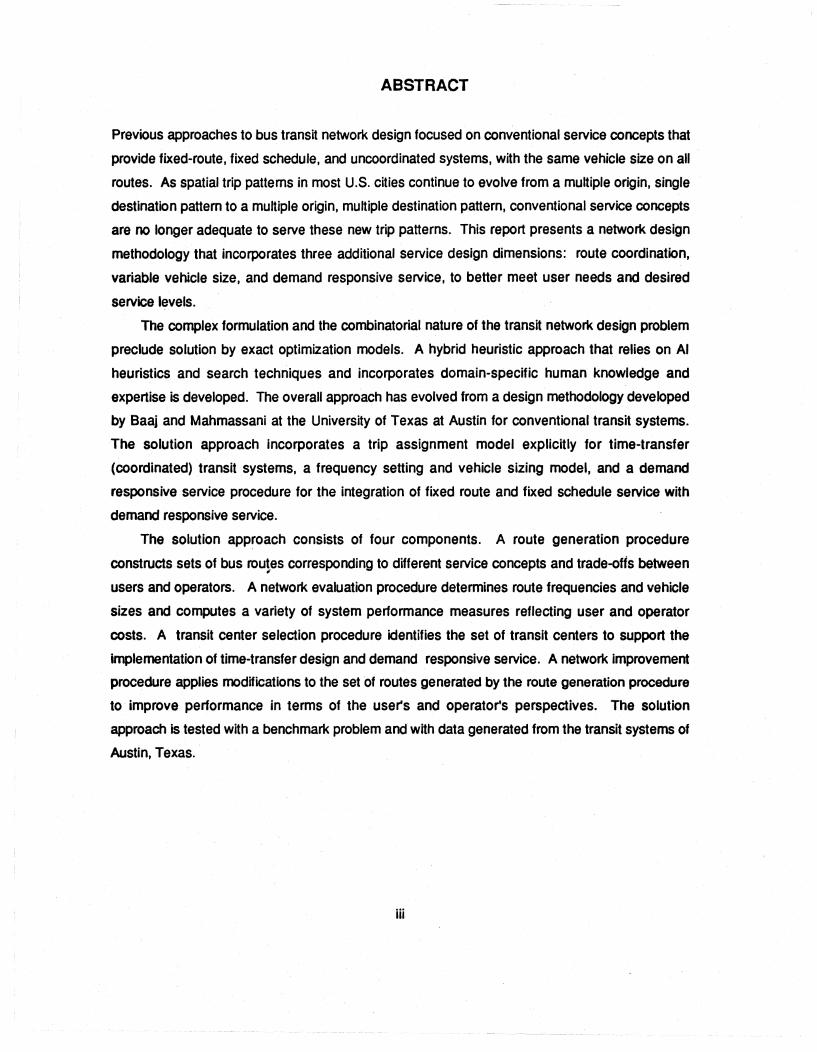
r-~:m_eport~_94/600_16-_1 _...L..--12. G_overnrne_nt Ac_ceUion_No. _-+--3. _"i'ifi,ijf 4. Title and Subtitle 5. Report Date A Design Methodology for Bus Transit Networks with Coordinated August 1994 Operations 6. Performing Organization Code
7. Author(s)
Mao-Chang Shih and Hani S. Mahmassani 9. Performing Organization Name and Address
Center for Transportation Research University of Texas at Austin 3208 Red River, Suite 200 Austin, Texas 78705-2650
12. Sponsoring Agency Name and Address
Southwest Region University Transportation Center Texas Transportation Institute The Texas A&M University System College Station, Texas 77843-3135
15. Supplementary Notes
8. Perfonning Organization Report No.
Research Report 600 16-1 10. Work Unit No. (TRAIS)
11. Contract or Grant No.
0079
13. Type of Report and Period Covered
14. Sponsoring Agency Code
SUpported by a grant from the Office of the Governor of the State of Texas, Energy Office 16. Abstract
"1Pa e
-
A major goal of transportation planning activities targeted at reducing total automotive fuel consumption has been to attract tripmakers to use public transit to meet more of their travel and mobility needs. Bus transit networks in the U.S. have traditionally been geared to serve centralized core-area land use patterns, at the same time that these cities have become increasingly decentralized. Because of lower suburban and exurban densities, it has been difficult to . provide levels of transit service that provide a meaningful alternative to the private automobile. However, increasing densification of the suburbs and the emergence of major activity nuclei outside the CBD opens opportunities for creative approaches to the supply of transit serVices.
The aim of this project is tq develop and test computer-based design procedures for the configuration of bus route networks in areas characterized by suburban spatial patterns, so as to maximize ridership capture and serve mobility needs in a cost-effective and energy efficient manner. The methodology incorporates three service dimensions that have heretofore been left out of systematic design procedures: route coordination, variable vehicle size and demandresponsive service. All three dimensions are particularly important in the design of transit service networks for areas encompassing significant suburban and exurban spatial development patterns.
The solution approach consists of four components. A route generation procedure constructs sets of bus routes corresponding to different service concepts and trade-offs between users and operators. A network evaluation procedure determines route frequencies and vehicle sizes and computes a variety of system performance measures reflecting user and operator costs. A transit center selection procedure identifies the set of transit centers to support the implementation of timed-transfer design and demand responsive service. A network improvement procedure applies modifications to the set of routes generated by the route generation procedure to improve performance in terms of the user's and operator's perspectives. The solution approach is tested with a benchmark problem and with data generated from the transit system of Austin, Texas.
17. Key Words 18. Distribution Statement
Transit Network Design, Suburban Mobility
No Restrictions. This document is available to the public through NTIS: National Technical Information Service 5285 Port Royal Road
19. Security Classif.{ofthis report)
Unclassified Form DOT F 1700.7 (8-72)
Springfield, Virginia 22161
\20. Security Classif.(of this page) 121. No. of Pages
Unclassified 197 I 22. Price
Reproduction of completed page authorized

A DESIGN METHODOLOGY FOR BUS TRANSIT NETWORKS WITH COORDINATED OPERATIONS
by
Mao-Chang Shih
Hani S. Mahmassani
SWUTC/94/60016-1
OPTIMAL DESIGN OF BUS TRANSIT NETWORKS FOR SUBURBAN MOBILITY NEEDS CONCEPTUAL FRAMEWORK AND MODEL DEVELOPMENT
Research Project 60016
conducted for the
Southwest Region University Transportation Center Texas Transportation Institute ,
The Texas A&MUniversity System College Station, Texas 77843-3135
Supported by a Grant for the Office of the Governor of the State of Texas, Energy Office
prepared by the
CENTER FOR TRANSPORTATION Bureau of Engineering Research
THE UNIVERSITY OF TEXAS AT AUSTIN
August 1994

,
ACKNOWLEDGEMENT
This publication was developed as part of the University Transportation Centers Program which is
funded 50% in oil overcharge funds from the Stripper Well settlement as provided by the Texas
State Energy Conservation Office and approved by the U,S. Department of Energy. Mention of
trade names or commercial products does not constitute endorsement or recommendation for,
use.
ii
-- ---...... ,--, .. __ . __ ._- -------- - --------. ----l----- -_.-
ABSTRACT
Previous approaches to bus transit network design focused on conventional service concepts that
provide fixed-route, fixed schedule, and uncoordinated systems, with the same vehicle size on all
routes. As spatial trip pattems in most U.S. cities continue to evolve from a multiple origin, Single
destination pattern to a multiple origin, multiple destination pattern, conventional service concepts
are no longer adequate to serve these new trip patterns. This report presents a network design
methodology that incorporates three additional service design dilnensions: route coordination,
variable vehicle size, and demand responsive service, to better meet user needs and desired
service levels.
The complex formulation and the combinatorial nature of the transit network design problem
preclude solution by exact optimization models. A hybrid heuristic approach that relies on AI
heuristics and search techniques and incorporates domain-specific human knowledge and
expertise is developed. The overall approach has evolved from a design methodology developed
by Baaj and Mahmassani at the University of Texas at Austin for conventional transit systems.
The solution approach incorporates a trip assignment model explicitly for time-transfer
(coordinated) transit systems, a frequency setting and vehicle sizing model, and a demand
responsive service procedure for the integration of fixed route and fixed schedule service with
demand responsive service.
The solution approach consists of four components. A route generation procedure
constructs sets of bus routes corresponding to different service concepts and trade-offs between "
users and operators. A network evaluation procedure determines route frequencies and vehicle
sizes and computes a variety of system performance measures reflecting user and operator
costs. A transit center selection procedure identifies the set of transit centers to support the
implementation of time-transfer design and demand responsive service. A network improvement
procedure applies modifications to the set of routes generated by the route generation procedure
to improve performance in terms of the user's and operator's perspectives. The solution
approach is tested with a benchmark problem and with data generated from the tranSit systems of
Austin, Texas.
iii

EXECUTIVE SUMMARY
Traditional bus systems, which provide primarily fixed-route, fixed-schedule and
uncoordinated service, has been targeted at serving centralized core-oriented land use patterns.
Over the pastfew decades, most U.S. cities have experienced continued spatial redistribution of
commercial development and population growth, with major peripheral commercial centers
becoming significant activity nodes outside of the traditional CBD. Population in most U.S. cities
has been growing much more rapidly in suburbs than in central cores. The resulting land use
pattern has transformed the associated spatial trip pattern from a multiple-origin, single
destination pattern for a multiple-origin and multiple-destination one, evidenced in metropolitan
areas like Houston and Dallas-Fort Worth.
Existing bus service systems that have resulted from successive incremental modifications
to the traditional network are neither effective nor efficient at serving the new spatial trip patterns
often resulting in user frustration and low ridership levels. While transit authorities have generally
recognized the problem, scientific tools and systematic procedures have not been available to
adequately support and facilitate attempts at major system redesign and re-engineering.
In particular, previous approaches and procedures have not been successful at incorporating
alternative service concepts that are particularly suitable for spatially dispensed demand patterns,
such as coordinated operation systems (e.g., time transfer systems), variable vehicle sizes (to
better match areas with lower ridership levels) and demand responsive service offered in an
integrated and complementary manner with conventional fixed-route service. , This report describes a systematic network design methodology that addresses the above
needs for a flexible approach that integrates the service concepts that have been shown to work
in lower density areas within an overall network of bus routes. Coordinated time-transfer service
allows greater coverage with limited eqUipment through expanded transfer capabilities with little
wait time at "hubs" with coordinated arrivals of buses from different routes. Variable bus sizes
allows greater flexibility in frequency resulting and in serving a variety of demand levels in
different markets. Demand-responsive service attempts to combine real-time operation' with
planned service in very low ridership areas.
The solution approach consists of four algorithmic procedures. The route generation
procedure (RGP) constructs sets of bus routes for designs with or without the transit center
concept. The network evaluation procedure (NETAP) determines route service frequencies and
vehicle sizes and evaluates transit systems for both coordinated and uncoordinated designs. The
transit center selection procedure (TCSP) identifies candidate sets of transit centers when the
iv

network is to be configured around the transit center concept. The network improvement
procedures (NIP) applies modifications to the set of routes generated by the RGP to improve
performance from the user's or operator's perspective.
Numerical experiments were performed to test the solution approach on a benchmark
problem. The results showed that networks generated by the RGP around the transit center
concept outperformed the solutions of Mandl's and Baaj and Mahmassani's algorithm. Numerical
experiments on data for the transit system of Austin, Texas, were also performed to test the
design procedures and investigate the performance of alternative design. The TCSP was tested
based on two application strategies and six selected combinations of demand satisfaction levels.
The tests indicated that the TCSP generated consistent results in all study cases. Transit centers
generated from the TCSP were either major activity centers or transit nodes within major
communities in the suburban areas. The RGP and NETAP were tested using four design
alternatives under six combinations of demand satisfaction levels. The tests compared the
performance of coordinated vs. uncoordinated networks. The tests also investigated the
performance of networks with the variable vehicle sizes vs. fixed vehicle size. The numerical
results showed that 1) the coordinated design resulted in better demand satisfaction levels, total
out-of-vehicle waiting time, and total system cost, but worse total in-vehicle travel time and total
travel time because additional in-vehicle waiting time was generated by the route coordination, 2)
designs of variable vehicle sizes greatly reduced the total system cost, fuel consumption, and out
of-vehicle waiting time, but increased the operation cost. Two possible NIP modifications were
tested. The procedure that splits routes at transit centers reduced the required operational
resources, but the levels10f demand satisfaction were decreased. The demand responsive
service procedure resulted in significant savings of operating resources and much lower
reductions in the level of demand satisfaction compared to outright route discontinuation.
v
TABLE OF CONTENTS
ACKNOWLEDGM ENTS ................................................................................................................... .ii
ABSTRACT .................................................................................................................................... .iii
EXECUTIVE SUMMARY ............................................................................................................... iv
TABLE OF CONTENTS .................................................................................................................. vi
LIST OF TABLES ............................................................................................................................ x
LIST OF FIGURES .......................................................................................................................... xi
CHAPTER 1. INTRODUCTION ... .................................................................................................. 1
PROBLEM DESCRIPTION AND MOTIVATION ...................................................................... 1
STUDY OBJECTIVES ............................................................................................................. 3
OVERVIEW .............................................................................................................................. 5
CHAPTER 2. LITERATURE REVIEW ........................................................................................... 7
OPTIMIZATION FORMULATIONS ......................................................................................... 7
HEURISTIC APPROACHES ... ................................................................................................ 7
Objective Function ............... : ............................................................................................. 8
Demand ............................................................................................................................. 8
Constraints ........................................................................................... '" ........................... 8
Passenger Behavior ................................................................................................... , ....... 9
Solution Techniques .......................................................................................................... 9
Decision Variables ....................................................................................... ; ................... 10 , Service Types .................................................................................................................. 10
Baaj (1990) ...................................................................................................................... 10
INNOVATIVE PRACTICES AND PRACTICAL GUIDELINES .............................................. 12
Transit Center Concepts .... .............................................................................................. 12
Timed-Transfer Coordinated Route Service .................................................................... 12
Demand Responsive Service ........................................................................................... 14
Variable Vehicle Sizes ...................................................................................................... 14
Practical Guidelines ......................................................................................................... 15
SHORTCOMINGS OF PREVIOUS APPROACHES .............................................................. 15
SUMMARY ............................................................................................................................. 18
CHAPTER 3. SOLUTION METHODOLOGY .............................................................................. 19
INTRODUCTION .................................................................................................................... 19
vi

SOLUTION FRAMEWORK AND ALTERNATIVE DESIGN FEATURES ............................... 19
THE ROUTE GENERATION PROCEDURE (RGP) ............................................................... 23
THE NETWORK ANALYSIS PROCEDURE (NETAP) ........................................................... 24
THE TRANSIT CENTER SELECTION PROCEDURE (TCSP) .............................................. 25
NETWORK IMPROVEMENT PROCEDURES (NIP) .............................................................. 25
ARTIFICIAL INTELLIGENCE (AI) SEARCH TECHNIQUES AND
DATA REPRESENTATION .......................................... 26
SUMMARY ..................... : ....................................................................................................... 27
CHAPTER 4. THE ROUTE GENERATION PROCEDURE ......................................................... 28
INTRODUCTION .................................................................................................................... 28
OVERVIEW OF THE RGP ...................................................................................................... 28
INPUT INFORMATION ............................................................................................................ 32
FORMATION OF INITIAL SKELETONS ................................................................................ 34
Selection of Initial Node Pair Seeds ................................................................................. 34
Construction of Initial Skeletons From Initial Node Pair Seeds ........................................ 35
EXPANSION OF SKELETONS TO ROUTES ........................................................................ 36
Order of Expansion .......................................................................................................... 37
Selection and Insertion of Feasible Nodes ....................................................................... 37
Route-Looping Test ................................................................................................... 39
Node-Sharing Test .................................................................................................... 39
Terminal Node Test ................................................................................................... 39
Route Circuity Test .................................................................................................... 39
Order of Node Insertion and Sorting Properties for Insertion .................................... 40
Termination of Route Expansion ...................................................................................... 41
Route Capacity Constraint ......................................................................................... 41
Route Length Constraint ............................................................................................ 42
SUMMARY OF RGP FEATURES .......................................................................................... 42
CHAPTER 5. THE NETWORK ANALYSIS PROCEDURE .......................................................... 44
INTRODUCTION .................................................................................................................... 44
OVERVIEW OF THE NETAP ................................................................................................. 45
INPUT INFORMATION ........................................................................................................... 48
TRIP ASSIGNMENT MODEL AND COMPUTATION OF NETWORK DESCRIPTORS ........ 48
Trip Assignment Characteristics in Timed-Transfer Systems .......................................... 51
vii
------ --- --- - ---.- ------ - --~-
I
Assignment Rules at Transfer Terminals ......................................................................... 51
Uncoordinated Operations Terminals ........................................................................ 52
Coordinated Operations Terminals with a Common Headway .................................. 53
Coordinated Operations Terminals with Integer-Ratio Headways ............................. 53
Missed Connections of Coordinated Routes ............................................................. 54
Trip Assignment Procedure for Timed-Transfer Systems ................................................ 57
Classification of Demand Node Pairs ........................................................................ 58
Assignment for O-Transfer Demand Pairs ................................................................. 59
Assignment for 1-Transfer Demand Pairs ................................................................. 59
Assignment for 2-Transfer Demand Pairs ................................................................. 60
Numerical Application to a Single Demand Node Pair ..................................................... 61
Trip Assignment for Integrated Bus Systems ................................................................... 64
Computation of Network Descriptors ............................................................................... 67
FREQUENCY SETTING AND VEHICLE SIZING PROCEDURE. .......................................... 67
Optimal Vehicle Size for Single Route with Given Demand ............................................. 70
Frequency Adjustment for Coordinated Routes ............................................................... 73
COMPUTATION OF SYSTEM PERFORMANCE MEASURES AND
CHARACTERIZATION OF NETWORK STRUCTURE ............. 74
Demand ........................................................................................................................... 74
User Costs ...... .................................................................................................................. 75
Level Service ...... .............................................................................................................. 76
Operator Cost ..... ~ ........................................................................................................... 76
Fuel Consumption ............................................................................................................ 76
System Utilization ............................................................................................................. 76
Network Structure Descriptor ..... ...................................................................................... n ILLUSTRATIVE APPLiCATION .............................................................................................. 78
Data Preparation ................................................................................ 00 ............................ 78
Results of RGP and NETAP lIlustrative Application ................... ................................ 00 •••• 81
SUMMARY ................................................................................................................. 00 .......... 86
CHAPTER 6. TRANSIT CENTER SELECTION PROCEDURE AND NETWORK
IMPROVEMENT PROCEDURES ................................................................ 87
INTRODUCTION .................................................................................................................... 87
THE TRANSIT CENTER SELECTION PROCEDURE (TCSP) .............................................. 90
viii
THE NETWORK IMPROVEMENT PROCEDURES (NIP) ..................................................... 93
Review of RIA Improvement Modifications ...................................................................... 94
Discontinuation of Service on Low Ridership Routes ................................................ 94
Route Joining ............................................................................................................. 94
Route Splitting ........................................................................................................... 95
Branch Exchange of Routes ...................................................................................... 96
Splitting Routes at Transit Centers .................................................................................. 96
Demand Responsive Service ........................................................................................... 97
Computation of Number of DRS Buses ......................................................................... 1 00
Numerical Example for the Demand Responsive Service Procedure ............................ 101
SUMMARY ........................................................................................................................... 105
CHAPTER 7. COMPUTATIONAL EXPERIMENTS ................................................................... 106
INTRODUCTION .................................................................................................................. 1 06
EXPERIMENTS ON BENCHMARK PROBLEM ................................................................... 107
Mandl's Transit Network .................................................................................................. 107
Numerical Results and Conclusions .............................................................................. 114
TESTS ON THE AUSTIN TRANSIT NETWORK ................................................................. 121
Tests of the TCSP .......................................................................................................... 126
Tests of the RGP and NETAP ........................................................................................ 126
Demand Satisfaction Levels .................................................................................... 128
User Travel Costs .................................................................................................... 128
Operation Costs ....................................................................................................... 140
Total System Cost ................................................................................................... 146
Computational Study of the Route Splitting Procedure for Coordinated Networks ........ 149
Experiments with the Integrated Bus System Design .................................................... 148
Summary of Tests on the Austin Transit Network .......................................................... 156
CHAPTER 8. CONCLUSIONS AND RECOMMENDATIONS .................................................... 158
SUMMARY AND CONCLUSiON .......................................................................................... 158
FUTURE RESEARCH .......................................................................................................... 160
APPENDICES ............................................................................................................................. 162
REFERENCES ............................................................................................................................ 182
ix
-- ---
I

LIST OF TABLES
2.1 Summary of Transit Network Design Models ...................................................................... 13
2.2 Suggested Service Planning Guidelines (Selected from NCHRP 69,1980) ...................... 17
4.1 Summary of Required Input Information for the RGP ......................................................... 34
5.1 Summary of Assignment Rules and Logic for Different Types of Transit Terminals ........... 52
5.2 Link Travel Times (minutes) and Route Frequencies (buses/hour)
for Example of Figure 5.3 .................................................................................................... 63
5.3 Path Links and Path Travel Cost for Example of Figure 5.3 ................................................ 63
5.4 Proportions of Demand Between Nodes i and j Assigned to Paths in All Cases ................ 64
5.5 Proportions of Demand Between Nodes i and j Assigned to Links in All Cases ................. 64
5.6 Route Information ................................................................................................................ 83
5.7 Summary of System Performance Measures ...................................................................... 84
5.8 Output Summary for Network Structure Descriptors ........................................................... 85
6.1 Node Information for the TCSP Illustrative Example ........................................................... 92
6.2 Shortest Travel Time Between Node Pairs for Network in Figure 6.3 .......... , .................... 103
6.3 New Demand Matrix for Fixed Route Service After the Reallocation
of Unsatisfied Demand ...................................................................................................... 103
7.1 Summary of Design Parameters for Three Test Cases .................................................... 113
7.2 Comparison of Solutions for the Benchmark Network for
Cases Using First Set of Design Parameters .................................................................... 117
7.3 Comparison of Solutions for the Benchmark Network for , Cases Using Second Set of Design Parameters .............................................................. 118
7.4 Comparison of Solutions for the Benchmark Network for
Cases Using Third Set of Design Parameters ................................................................... 119
7.5 User Specified Parameters for Experiments on the Austin NetwOrk ................................ 123
7.6 Six Selected Combinations of Minimum System Coverage and Directness Levels .......... 124
7.7 Sets of Transit Centers Generated by Single Pass and Iterative Application of TCSP for
Different Combinations of Minimum System Coverage and Directness Levels ............... 125
7.8 Comparison of Network CharacteristiCs for Different Route
Splitting Ratios at Transit Centers .................................................................................... 149
7.9 Network Characteristics for Integrated Bus Systems with
Uncoordinated Route Operations ...................................................................................... 153
7.10 Network Characteristics for Integrated Bus Systems with
Coordinated Route Operations ......................................................................................... 155
x
LIST OF FIGURES
3.1 Solution Approach ................................................................................................................ 21
3.2 Conventional Uncoordinated Bus System Design ............................................................... 22
4.1 Route Generation Procedure (RGP) ................................................................................... 31
4.2 Route Expansion Procedure ............................................................................................... 38
5.1 Network Analysis Procedure (NET AP) ................................................................................ 49
5.2 Vehicle Availability at a Coordinated Terminal .................................................................... 55
5.3 Example Route Network with Six 1-Transfer Paths ............................................................. 62
5.4 Transit Centers for Austin Study Case ................................................................................ 80
5.5 Output Summary for Application of the RGP ....................................................................... 81
6.1 Transit Center Selection Procedure (TCSP) ....................................................................... 91
6.2 Demand Responsive Service Procedure ............................................................................ 99
6.3 Network and Transit Demand Matrix for the Illustration
of the Demand Responsive Service Procedure ................................................................ 102
6.4 Candidate Demand Responsive Service Routes for the Illustrative Example ................... 104
7.1 Mandl's Swiss Network and Transit Demand Matrix ......................................................... 108
7.2 Route Layout Generated by Mandl's Algorithm ................................................................. 109
7.3 Route Layout Generated by Baaj and Mahmassani's
RGA for First Set of Design Parameters ........................................................................... 110
7.4 Route Layout Generated by Baaj and Mahmassani's
RGA for Second Set of Design Parameters ....................................................................... 111 , 7.5 Route Layout Generated by Baaj and Mahmassani's
RGA for Third Set of Design Parameters .......................................................................... 112
7.6 Route Layout Generated by RGP for First and Third
Set of Design Parameters ................................................................................................. 115
7.7 Route Layout Generated by RGP for Second
Set of Design Parameters ................................................................................................. 116
7.8 Percentage of Demand Satisfied Directly vs. Minimum
System Directness Level ...................................................................................... , ............ 127
7.9 Percentage of Demand Satisfied with One Transfer vs.
Minimum System Directness Level ................................................................................... 129
7.10 Percentage of Total Demand Satisfied vs. Minimum
System Dfrectness Level ........................................................... ~ ....................................... 130
7.11 Total In-Vehicle Travel Time vs. Minimum System Directness
xi
Level for Minimum System Coverage Level = 80% ......................................................... 131
7.12 Total In-Vehicle Travel Time vs. Minimum System Directness
Level for Minimum System Coverage Level:: 98% ......................................................... 132
7.13 Average Passenger In-Vehicle Travel Time vs. Minimum System
Directness Level for Minimum System Coverage Level = 80% ...................................... 134
7.14 Average Passenger In-Vehicle Travel Time vs. Minimum System
Directness Level for Minimum System Coverage Level = 98% ...................................... 135
7.15 Total Out-of-Vehicle Waiting Time vs. Minimum System
Directness Level for Minimum System Coverage Level = 80% ...................................... 136
7.16 Total Out-of-Vehicle Waiting Time vs. Minimum System
Directness Level for Minimum System Coverage Level = 98% ...................................... 137
7.17 Average Passenger Out-of-Vehicle Waiting Time vs. Minimum
System Directness Level for Minimum System Coverage Level:: 80% ......................... 138
7.18 Average Passenger Out-of-Vehicle Waiting Time vs. Minimum
System Directness Level for Minimum System Coverage Level = 98% .......................... 139
7.19 Total Transfer Penalty vs. Minimum System Directness Level ...................................... 141
7.20 Total Travel Time vs. Minimum System Directness Level .............................................. 142
7.21 Total Fuel Consumption vs. Minimum System Directness Level
for Minimum System Coverage Level:: 80% .................................................................. 143
7.22 Total Fuel Consumption vs. Minimum System Directness Level
for Minimum System Coverage Level = 98% .................................................................. 144
7.23 Total Operation Cost vs. Minimum System Directness Level ........................................... 145
7.24 Total System Cost vs. Minimum System Directness Level ............................................... 147
7.25 User Travel Times VS. Splitting Ratio ................................................................................ 150
7.26 System Costs VS. Splitting Ratio ....................................................................................... 151
xii
-~--- -- -- ----- -- - - ------ --r-- '"---- --- ------

CHAPTER 1. INTRODUCTION
PROBLEM DESCRIPTION AND MOTIVATION
The significance of public transportation is revealed in several aspects. In addition to
providing mobility to people who have no other options (e.g. people who do not own a car, cannot
afford to drive, or are physically unable to drive), public transportation offers travel alternatives to
those who might use transit for the reasons of cost, speed, comfort, convenience, traffic
avoidance, or environmental principle. Public transit has been recognized as part of the solution
to the growing vehicular traffic congestion problem on overloaded urban transportation systems.
Increased reliance on public transit systems has been advocated as an efficient way of lowering
energy consumption and reducing air pollution.
Among all transit modes, bus transit is the dominant form in American cities. As indicated in
the Transit Fact Book (1991), more than 65% of the 8.9 billion annual transit trips in the US were
bus trips. Buses account for almost 50% of the 41.5 billion annual transit passenger miles. In
addition, there are about 2,700 bus systems in the US, of which more than one-fourth are in
urbanized areas of less than 50,000 people.
The process of developing a bus service plan consists of five stages: network design,
frequency setting, timetable development, bus scheduling and driver scheduling (Ceder and
Wilson, 1986). The bulk of past research effort has been concentrated on bus scheduling and
driver scheduling. This is understandable because these two activities are directly reflected in the
operating cost and are rf.adily amenable to computer-based procedures. However, the two most
fundamental elements, namely, the design of bus routes and setting of frequencies, which
critically determine the system's performance from both the operator's and users' point of view,
have not been sufficiently investigated because of their inherent complexity and implementation
difficulty.
Baaj (1990) pointed out five main sources of complexity that preclude finding a unique
optimal solution for the transit network design problem: difficulty of formulating the problem; non
linearity and non-convexity of the mathematical formulation; inherent combinatorial complexity of
the problem; multi-objective nature of the problem; and spatial layout of routes. Although
decision variables such as frequency, vehicle size, and route space can be expressed in the
problem formulation, the number of routes and their nodal composition are difficult to define. In
addition, transit trip assignment, used to determine route demands for a bus system, cannot be
expressed in a well-behaved mathematical formulation. Due to the discrete nature of the route
selection problem, the choice of routes is generally a non-convex optimization problem (or an
1
integer programming problem), and the selection of an optimal route structure is an NP-hard
combinatorial problem (Newell, 1979). Most approaches for the transit network design problem
consider operator cost and/or user cost as their objectives. In practice, service coverage, service
directness, and other conflicting objectives are examined in the design process. This implies that
conflicting objectives need to be addressed. Finding acceptable and good spatial layout of
routes should satisfy important criteria such as route coverage, route duplication, route length,
and directness of route. All the above factors contribute to the difficulty of solving the transit
network design problem.
Traditional bus systems have been targeted to serve centralized core-oriented land use
patterns. These bus systems provide fixed-route, fixed-schedule, and uncoordinated service,
and are either radial- or grid-like. Most of the current bus transit systems in the US have evolved
largely from the traditional systems, and their networks have been carried over from old streetcar
operation. Expansion or deletion of elements of the bus network are highly dependent on the
transit planners' judgment, experience, and knowledge of the existing land use patterns, demand
patterns, service requirements, and resource constraints.
In recent years, most U.S. cities have experienced spatial redistribution of commercial
development and population growth. Capitalizing on lower land values and ability to avoid traffic
congestion in the downtown area, major peripheral commercial centers have been developed
outside the central business district. In the same manner, population in most U.S. cities has been
growing much faster in suburbs than in central cores. The resulting land use pattern of
increasingly decentralizep cities has transformed the associated spatial trip pattern from a multiple
origin, single destination pattern to a multiple origin, multiple destination one, evidenced in
metropolitan areas like Houston or Dallas-Fort Worth.
Existing bus service plans that have resulted from successive incremental modifications to
the traditional network are neither effective nor efficient at serving the new spatial trip patterns,
and often result in user frustration, and consequently low ridership. A nationwide survey showed
that only two percent of all suburban employees commute to work by bus (Cervero, 1986). The
failure to provide meaningful alternatives to the private automobile in most cities has resulted in
heavy reliance on the private automobile as the only available means of mobility. The
consequences are intensified traffic congestion, wasteful fuel consumption, and magnified air
pollution. Some transit authorities have recognized the existing problem. However, attempts at
major reevaluation and redesign have not been supported and guided by scientific tools or
systematic procedures.
Previous approaches for the transit network design problem have focused on the design of
2

conventional bus service, which provides fixed-route, fixed-schedule, and uncoordinated route
service. Such service is no longer adequate to serve cities with a multi-centered and spatially
dispersed trip pattern. Alternative design concepts, especially coordinated route service,
demand responsive service, and variable vehicle sizes, have been proposed and implemented in
several cities in North America and Europe with some encouraging results. The need for
innovative modeling concepts to design bus transit networks is thus apparent.
The principal problem addressed in this study is how to redesign a bus transit network
around a different service philosophy that recognizes the changing nature of the land use and
associated travel activities. The intent is to design a bus route network and service plan that
provides cost-effective quality public transportation (in terms of frequency, directness, comfort,
and coverage) under the consideration of resource availability.
STUDY OBJECTIVES
. The goal of the proposed work is to develop computer-based design procedures which
incorporate alternative design concepts to provide good solutions to the bus transit network
design problems encountered by the transit industry today. Reaching this goal entails fulfilling
the following objectives:
1) To identify superior transit network designs and service planning options for the type of
spatial trip pattern that prevails in most North American cities.
2) To develop and test a set of algorithmic design procedures which incorporate current
practice and !!xisting rules-of-thumb with regard to bus network design, to account for
the above options.
3) To incorporate the capability to evaluate performance from both passenger and
operator perspectives for various service options. In other words, the transit network
evaluation model should possess the capability to determine various system
performance measures which explicitly recognize the multi-objective nature of the
transit network design problem.
4) To perform systematic assessments of alternative service design concepts and of the
associated trade-offs in order to ascertain the conditions that determine their success.
The complex formulation and the combinatorial nature of the transit network design problem
preclude solutions by exact optimization models. Baaj and Mahmassani (1991) developed a
hybrid solution approach that included the following major features: 1) AI-based heuristic
procedures for transit route generation and improvement, 2) a transit network evaluation model to
analyze transit system performance in consideration of the multi-objective nature of transit
3

network design, and 3) the use of domain-specific knowledge reflecting current practice and
existing rules of thumb concerning design issues. Their model is applicable to design of
conventional fixed-route, fixed-schedule, uncoordinated bus systems with the same vehicle size
on all routes.
In this report, the above hybrid heuristic approach is extended and further developed to
provide alternative design concepts and features oriented towards the kind of land use and transit
demand patterns found in most u.s. cities. These design concepts include conventional
systems with fixed-route, fixed-schedule, and uncoordinated route service; timed-transfer
systems with coordinated route service; and integrated systems with conventional service for high
demand areas and demand responsive service for low density areas. In addition, a variable bus
size option is available with the above design concepts. Four algorithmic procedures are
developed to provide these design features, namely, the route generation procedure, the
network analysis procedure, the transit center selection procedure, and the network improvement
procedure.
This solution approach differs from existing approaches, including Baaj and Mahmassani's, in
the following meaningful aspects:
1) Ability to identify transit centers. The transit center selection procedure incorporates
criteria reflecting land use pattern, transit demand, service coverage, and transfer
opportunity at transit centers.
2) A route network that is heavily guided by the demand matrix, and configured with the
transit center c9ncept. The route generation procedure produces route networks that
serve the demand pattern and provide good transfer opportunities at transit centers, as
well as fast and direct service between transit centers.
3) Provision of alternative design concepts including conventional, coordinated, and
integrated bus systems. The timed-transfer concept is intended to reduce the negative
impact of transfers. Demand responsive service provides more effective service to low
demand density areas than conventional fixed-route, fixed-schedule service.
4) Ability to evaluate coordinated bus operations. The network evaluation procedure assigns
trips for both coordinated and uncoordinated transit systems.
5) Variable vehicle size option, which provides an additional choice dimension in designing
the service configuration to better meet user needs and desired service levels.
6) A route splitting modification for coordinated systems to improve resource effectiveness.
In addition, the solution approach provides a framework to incorporate applicable service planning
guidelines as well as knowledge and expertise of transit planners. Consequently, acceptable and
4

operationally implementable route networks and service plans are designed.
OVERVIEW
In this chapter, the significance of transit network design in the context of transit planning
activities has been described, and the study's objectives and general approach have been
defined accordingly.
In Chapter 2, an in-depth background review of the transit network design problem is
presented together with innovative concepts and practical guidelines for the design of bus
networks and the provision of bus service. Previous approaches to the transit network problem
are reviewed with regard to seven distinguishing features: objective function, demand,
constraints, passenger behavior, solution techniques, decision variables, and service types.
Shortcomings of these approaches are discussed as well.
Chapter 3 presents the solution framework which consists of four main procedures: the route
generation procedure, the network analysis procedure, the transit center selection procedure,
and network improvement procedures. An overview of these four procedures is presented. The
design features that are provided by the solution approach are described as well. In addition, the
motivation for implementing the procedure in the LISP computer language, intended primarily for
artificial intelligence applications, is described.
Chapter 4 presents the details of the route generation procedure (RGP). It describes three
main components, including the formation of initial skeletons, the expansion of skeletons to
complete routes, and thp termination of the RGP. Required input information for executing the
RG P is described as well as the RG P's important features which ensure the generation of quality
route networks.
Chapter 5 covers the network analysis procedure (NETAP). The NETAP is used to evaluate
alternative bus network and service plans; it is also utilized to determine route frequencies and
vehicle sizes for a given route network. The required input information for the execution of the
NETAP are described as well as the resulting output that includes a variety of performance
measures. The details of two main components of the NETAP, namely the trip assignment
procedure and the frequency setting and bus sizing procedure are presented in detail. The
chapter concludes with an illustrative application to the Austin transit network.
Chapter 6 presents the transit center selection procedure (TCSP) and network improvement
procedures (NIP). The TCSP identifies suitable transit centers for the design of coordinated
timed-transfer systems and the implementation of demand responsive service. The TCSP
incorporates guidelines commonly used in the transit industry to select transit centers. The NIP
5
improves the set of routes generated by the RGP via several possible modifications including
discontinuation of service on low ridership routes, joining of routes, splitting of routes, branch
exchange of routes, splitting of routes at transit centers, and implementation of demand
responsive service.
Chapter 7 focuses on testing the design procedures and different design alternatives
provided by the solution framework. Tests are conducted on an existing benchmark problem and
on data generated from the transit network of Austin, Texas. Results of the different tests are
presented and analyzed. Chapter 8 presents the conclusions from the research results and
discusses directions for future· research.
,
6
CHAPTER 2. LITERATURE REVIEW
Previous solution approaches to the bus transit network design problem can be categorized
into optimization formulations that deal primarily with idealized situations, and heuristic algorithms
for more realistic problems. In the subsequent sections, both types of approaches are reviewed.
In addition, innovative practices that produce satisfactory solutions and practical guidelines that
reflect operational feasibility are identified in relation to this study.
OPTIMIZATION FORMULATIONS
Existing optimization formulations of the transit network design problem are concerned
primarily with the minimization of a generalized cost measure, usually a combination of user costs
and operator costs. In most studies, user costs consist of access cost, waiting time cost, and in
vehicle travel time cost; operator cost is estimated by total vehicle operating miles or time.
Feasibility constraints may include, but are not limited to 1) minimum operating frequencies on all
or selected routes, 2) a maximum load factor on bus routes, and 3) maximum available resources
(fleet size or capital).
Due to the sources of complexity of the transit network design problem described in the
previous chapter, optimization methods were only applied to determine one or several design
parameters (e.g. route spacing, route length, stop spacing, bus size, and headway) on a
predetermined route structure, rather than determine both the route structure and design
parameters simultaneously. Examples of optimization approaches include the work of Oldfield
and Bly (1988), LeBlanc (1988), and Chang (1990). Consequently, heuristic approaches that do , not guarantee a global optimal solution have been proposed to solve the transit network design
problem.
HEURISTIC APPROACHES
Heuristic approaches include those of Lampkin and Saalmans (1967), Rea (1971). Silman, et
al. (1974), Mandl (1979), Dubois, et al. (1979), Hasselstrom (1981), Ceder and Wilson (1986), Van
Nes, et al. (1988), Baaj (1990), and Israeli and Ceder (1991). A thorough review of previous
approaches to the bus network design problem has been conducted by Baaj. His review
identifies five distinguishing features that characterize these approaches: objective function,
demand, constraints, passenger behavior, and solution techniques. In this study, two additional
features are included: decision variables and service type. In the following synthesis, each of the
seven features is discussed individually by comparing the previous heuristic approaches and
defining the most appropriate feature for the transit network design problem.
7

Objective Function
Most previous approaches seek to minimize generalized cost (user cost and/or operator
cost)). Hasselstrom proposed maximizing consumer surplus to cope with variable demand, while
Van Nes et al. maximize the number of direct trips. Instead of specHying an objective function,
Rea's model seeks a solution which meets certain operator-specified pertormance levels. Baaj
points out the importance of addressing the multi-objective nature of the transit network design
problem. In Baaj's model, the total demand satisfied and its components (the total demand
satisfied directly, via one transfer, via two transfer, or unsatisfied) are examined against the total
travel time and its components (the total travel time that is in-vehicle, waiting, or transferring), as
well as against the fleet size required to operate the system (as a proxy measure for operator cost).
Israeli arld Ceder consider the minimization of generalized cost and fleet size in their two objective
formulation.
Demand
Demand is an essential element for transit network design. In previous approaches, except
Dubois et aI., Hasselstrom, and Van Nes et al., demand is assumed fixed and independent of
service quality. Dubois et al. use a diversion curve based on expected travel times to estimate the
public transport share from the total trip matrix. In Hasselstrom's model, a direct model is used to
estimate a demand matrix for both high quality service throughout the area and less than ideal
service between some origin-destination pairs. Van Nes et al. employ a direct demand model
based on the simultaneous distribution-modal split model. Conceptually, the variable demand
assumption is more appealing. However, the questionable accuracy of existing demand models
and the added complexity of using variable demand models make the fixed demand formulation
more useful practically.
Constraints
Constraints on the total operator cost, fleet size and service frequency are common to
several previous approaches. Total operator cost and fleet size constraints are thought to be
interchangeable since the operating cost is highly correlated with the required vehicle-miles and
vehicle-hours of operation, and the number of vehicles that are needed in the service is also
directly affected by the required vehicle-miles and vehicle-hours of operation. A minimum
frequency is applied to provide meaningful bus service. Instead of generating real numbers for
bus frequencies, Van Nes et al. use a set of possible integer-valued frequencies. The use of fleet
size and service frequency constraints requires that bus allocation and frequency setting sub
problems be solved simultaneously with the transit network design problem. Baaj has
8
-------- -r------- ------- ----- ---- ---

successfully implemented other service-related constraints that include the route round trip time,
the directness of routes as measured by a circuity factor, load standard, and the route ridership
volume. These constraints are crucial to providing quality transit service.
Passenger Behavior
Passenger behavior is reflected in the transit trip assignment formulation assumed in a
particular approach. As Ceder and Wilson noted, previous transit trip assignment models can be
divided into two groups, namely, single path assignment and multiple path assignment. Rea and
Mandl follow single path assignment of all passengers to the least weighted cost path. All other
approaches utilize multiple path assignment models that first define a set of acceptable paths, and
then assign a proportion of passengers to each acceptable path equivalent to the probability that
the first bus to arrive serves that path. The difference in these multiple path assignment models is
the definition of path acceptability. Multiple path assignment is thought to be more appropriate for
transit trips because it accounts for the waiting phenomenon at transit terminals with multiple
acceptable routes.
Solution Techniques
To overcome the complexity of transit network deSign, most previous approaches partition
the problem into two parts, route construction and frequency setting. Mandl and Baaj add a route
improvement procedure to improve the initial network. Most other approaches, except those of
Hasselstrom and Van Nes et al., determine route structure and assign frequencies separately by
first obtaining an initial reasonable route network, and then applying mathematical formulations to ~
solve for route frequencies. The models of Lampkin and Saalmans. Silman et al.. Dubois et aI.,
and Baaj all use a route generation procedure that starts from initial route skeletons generated by
candidate nodes. Among them. Baaj's model considers demand as the criterion for selecting the
initial skeletons. Additional nodes are added to these skeletons by following given insertion
criteria to form complete routes. Silman et al. generate many more routes than will actually be
operated. and rely on the frequency allocation procedure to define the route network .. The
models of Mandl and of Rea both focus on the acceptability of links that are then aggregated to
form routes. Israeli and Ceder enumerate all possible routes from preset termini and apply a route
length constraint to eliminate routes with travel time. between each origin-destination (0-0) pair.
exceeding the least-time path by a given threshold.
Hasselstrom uses a complex two-level optimization model which first reduces the network by
eliminating links that are seldom or never used by passengers. A large set of possible routes is
then generated from the remaining links. Finally, the network routes are selected by assigning
9

frequencies using a linear programming model which maximizes the number of transfers saved by
changing from a link network (transfers at every node) to a public transit network (transfers only at
intersections). Van Nes et al. assign frequencies to a pre-selected set of possible routes and
increase the frequency on the route with the highest efficiency ratio, defined as the ratio of the
number of extra passengers as a result of the increase to the associated cost of the increase.
They point out that the ratio can be regarded as an estimate of the Lagrange multiplier of the
optimization formulation which maximizes the number of direct trips with a given fleet size.
Decision Variables
All previous approaches except Mandl's consider route and frequency as their decision
variables. Mandl assumes a constant frequency on all bus routes. Although this assumption
simplifies the network design problem, using the same frequency on all bus routes is unrealistic.
All other approaches fix the vehicle size, and use frequency as the only variable in the resource
allocation process. In the transit industry, different vehicle sizes have been implemented on
routes having different passenger volumes or providing different types of services. It is desirable
. to treat vehicle size as a decision variable in the design procedure.
Service Types
All previous approaches have focused on conventional transit service, which provides fixed
route, fixed-schedule, and uncoordinated-route service. Such service is suitable for areas with
high demand density and single-centered trip patterns, but is ineffective in serving areas with low
demand density and multiple-centered trip patterns. Other service types, especially those that #
can better serve low demand density areas (e.g. timed-transfer systems and demand responsive
bus services) should be identified and incorporated in the overall bus network design.
Of the models discussed earlier, Baaj's model is presented in more detail for the following
reasons:
1) Baai's route generation procedure is highly responsive to the transit demand matrix.
2) The model effectively incorporates practical guidelines such as route length,
frequency, route duplication, route directness, and load standard.
3) The model will provide a benchmark to the solutions resulting from this study.
4) The overall approach of this study has evolved from and extends Baaj's model.
Baal (1990)
Baai's approach consists of three parts. The first part is a route generation algorithm (RGA)
which generates sets of good routes that correspond to different trade-offs between user cost
10
""T ------- - --- -- ----- -~---
and operator cost. The second part is a transit route analysis procedure (TRUST) to evaluate a
given transit network and set route frequencies for a new transit network design. The last part is
the route improvement algorithm (RGA) which improves the initially generated sets of routes.
1. RGA starts by selecting high demand node pairs to form the initial set of skeletons. The
skeleton of each node pair consists of either the shortest path connecting the corresponding
node pair or an aHemate path between them. TheaHernate path for a given node pair satisfies
two criteria: (1) it should not be too long; and (2) its nodal composition should be substantially
different from that of the shortest path. Among all acceptable paths, one may select either the
path covering more network nodes or the shortest path. Each skeleton is then expanded by
inserting the set of feasible nodes. These· feasible nodes need to satisfy the following six
conditions:
1) Nodes do not belong to the route under expansion.
2) Nodes still have a high percentage of their total originating demand left unsatisfied after
insertion in other routes.
3) The resuHing route does not become circuitous.
4) The ratio of the contributed demand satisfied per insertion cost exceeds a minimum
demand per insertion cost value.
S) The required. frequency of service on the resulting route does not exceed the
maximum operationally implementable value.
6) The length of the resuHing route does not exceed a maximum allowable value.
The route generation algorithm continues to generate routes until both the total demand satisfied
and the total demand satisfied directly exceed the user specified levels.
2. TRUST performs the passenger trip assignment and the frequency setting after the set of
routes is generated. The given demands between origin-destination pairs of the generated
network are first assigned based on assumed initial frequencies of service on all routes. The
frequency required on each route to maintain the load factor under a user pre specified
maximum is then computed. If the resulting frequencies are significantly different from the
initial values, TRUST reiterates with the output frequencies as the input frequencies until they
converge to the same values.
3. RIA makes the following modifications to improve the set of initially generated routes so as to
obtain feasible and implementable route networks.
1) Discontinue low ridership and/or short routes.
2) Merge low ridership and/or short routes with other routes if they can be merged.
11

3) Split routes with one-way in-vehicle travel time exceeding one hour into two routes.
4) Apply a branch exchange heuristic to form a new combination of routes so as to reduce
the number of transfers.
Table 2.1 summarizes all previous solution approaches discussed in this section.
INNOVATIVE PRACTICES AND PRACTICAL GUIDELINES
Transit Center Concepts
Several communities around the US. Canada. and Europe have proposed and implemented
some promising approaches which provide suitable service to multi-nucleated metropolises with
extensive suburban development. Most of these approaches revolve around the concept of
transit centers, consisting of major community retail and/or employment centers, that function as
effective hubs around which operations are structured. These centers are served by feeder bus
or by paratransit. usually some form of demand responsive operation that accomplishes a regional
collection-distribution function, as well as by trunk or main lines that interconnect the various
centers. Schneider and Smith (1981) suggested general guidelines for the selection of such
potential centers which include transit demand. area geometry, accessibility. and network
structure. Their concepts have been implemented in the Seattle. Washington. area with positive
results. The hubbing approach is also seen in many other cities such as Orange County.
California; San Diego. California; Eugene. Oregon; Vancouver. Canada; and London. England.
Timed· Transfer Coordinated Route Service
The major disadvankige of the hubbing approach is that it might require passengers to
transfer in order to complete their trips. To minimize the negative effect of transfer on ridership,
the concept of timed-transfer, whereby bus schedules are coordinated at transit centers to
provide for almost simultaneous (typically within a time window of 2 to 5 minutes) arrival of transit
vehicles from different routes, has been proposed to reduce the transfer waiting time. To ensure
synchronization, all routes must operate on the same or multiple integer headways. Accurate
. schedule and fairly reliable service are needed to insure the operational success of timed
transfers. Several existing transit systems have implemented the timed-transfer concept. The
commonly given example of a successful North-American system is in Edmonton, Alberta
(Canada). In the US, Portland, Oregon, has also introduced the timed-transfer concept at a few
suburban transit centers with generally positive results (Tri-County MTD, 1982).
Although timed-transfers can reduce the waiting time incurred by transferring users, the
potentially significant negative impact on existing ridership cannot be eliminated when systems
12

Year Author Objectives Demand Trip Decision Solution Service Type Assignment Variables Techniques
1961 Lampkin and Generalized Fixed Multiple Route and Sequential Fixed-route, fIXed-schedule Saalmans time frequency and uncoordinated-route
1972 Rea '" Fixed Single Route and Sequential Fixed-route, fixed-schedule frequency and uncoordinated-route
1914 Silman, Barzily. Generalized Fixed Multiple Route and Sequential Fixed-route, fixed-schedule andPassy cost frequency and uncoordinated-route
... 1916 Mandl Generalized Fixed Single Route Sequential Fixed-route, fixed-schedule
time and uncoordinated-route
1919 DuboiS., Bell, Generalized Fixed Multiple Route and Sequential Fixed-route, fixed-schedule andLli re time frequency and uncoordinated-route
1981 Hasselstrom Consumer Variable Multiple Route and Simultaneous Fixed-route, fixed-schedule surplus frequency and uncoordinated-route
1986 Ceder and Generalized Fixed Multiple Route and Sequential Fixed-route, fixed-schedule ..... Wilson""" time frequency and uncoordinated-route (.\)
1988 Van Nes, Number of Variable Multiple Route and Simultaneous Fixed-route, fIXed-schedule Immersi and direct trips frequency and uncoordinated-route Hamers ag
1990 Baaj *"'* Fixed Multiple Route and Sequential Fixed-route, fixed-schedule frequency and uncoordinated-route
1991 Israeli Generalized Variable Multiple Route and Sequential Fixed-route, fIXed-schedule Wilson time. and frequency and uncoordinated-route
fleet size
*: No exclicit objective function, but generated solutions meet certain operator specified performance levels "'*: Prob em formulation only . *"'''': Multi-objective approach. generates solutions reflecting trade-offs among objectives
Table 2.1 Summary of Transit Network Design Models

are re-structured around transit centers. As indicated by Newman et a!. (1983), the major source
of ridership concern is the increase in the number of required transfers across most trips. Part of
the problem arises from the procedures typically followed to design routes around the transit
center concept. These have been driven by the need to ensure compatible vehicle cycles on the
various routes. In addition to the increased number of transfers, timed transfer systems increase
travel time for passengers who remain on board at the centers and thus must wait for the duration
of an entire time window to accommodate transfer requirement. Therefore, the planner should
examine the trade-ofts between conflicting objectives in the design and implementation of timed
transfer systems.
Abkowitz et al. (1987) pointed out that operational feasibility of timed transfer in transit
systems depends on the compatibility between scheduled headways and congestion levels
along the route. Coordination of routes with incompatible headways results in ineffective
resource allocation. Implementation of the timed-transfer concept for routes serving areas with
high congestion levels is undesirable, because travel time variability and randomness due to
deviations from synchronized schedules could have severe impacts on the quality of service of
timed-transfer systems. It is essential to have reliable data regarding travel time for the
implementation of timed-transfer systems (Bakker, Calkin, and Sylvester, 1988).
Demand Responsive Service
Recognizing the ineffectiveness of fixed-route bus service for low-density areas, the transit
industry in the US has introduced demand responsive bus services. As of May 1991, about
3,900 transit systems operated demand responsive services (Transit Fact Book, 1991). Normally,
the use of demand responsive instead of fixed-route bus services in low-density areas will
increase transit ridership, expand transit system coverage, and provide more effective operation.
Several existing transit systems integrate demand responsive bus services with fixed-route bus
services so that fixed bus routes serve high-density areas and demand responsive buses serve
low-density areas. Examples of such integrated operation include Ann Arbor, Michigan, and
Santa Clara County, California. Both systems have experienced various levels of success (Chang
and Schonfeld, 1991).
Variable Vehicle Sizes
Due to high labor costs, transit operators in both Europe and North America tend to utilize
fewer but larger buses to provide the capacity required during peak period operation. Although
smaller buses cost more to operate per seat provided, their use may offer several advantages in
14
.. !
some ciraJrnstances. Glaister (1985) argued that the use of small vehicles favors the provision of
higher service frequencies, thereby lowering average wait times, and results in higher operation
speed; the improved service levels can be expected to generate new demand for bus transit.
Furthermore, smaller buses may be better suited for some types of service, such as Iow-demand,
low-occupancy, high-quality,or special transit, as suggested by Oldfield and Bly (1988). Smaller
vehicles are more acceptable to residents of certain low-density neighborhoods, and tend to
cause less pavement damage on city streets. Other reasons for using different vehicle sizes are
suggested by Walters (1979), Mohring (1983), Bly and Oldfield (1986), and Glaister (1986). To
the extent that a given service area includes zones with different demand densities, allowing
different vehicle sizes to operate on different bus routes and provide various types of services
provides the transit operator with an additional· choice dimension in the design of a service
configuration which meets user needs better and provides desired service levels.
Although both vehicle size and route frequency are important elements of bus service plans,
all previous bus network design procedures treat vehicle size as a fixed value and compute route
frequency either to achieve a minimum total generalized cost or to provide the capacity needed
during peak hour operation. The use of a fixed vehicle size simplifies the network design
procedure, but precludes the simultaneous consideration of various vehicle sizes in the bus
system design, and thus may result in ineffective resource allocation.
Practical Guidelines
Practically, transit service plans rely greatly on service planning guidelines that are mainly
based on the practical experience and professional judgment of transit planners rather than on
theoretical considerations. NCHRP 69 (1980) suggested constructing transit service guidelines
based on interviews with transit agencies over a broad spectrum of US and Canadian cities.
Particularly important guidelines for transit network design are those pertaining to the service
pattern and service levels; these are summarized in Table 2.2. Although service planning
guidelines are not sufficient to provide a complete solution to the design problem, violation of
these guidelines may cause infeasible or ineffective operation. Properly incorporating service
planning guidelines into the design model would result in a more operationally acceptable route
design and service plan. Baaj (1990) pointed out that most other approaches fail to incorporate
practical guidelines,and consequently have difficulty being accepted by the transit industry.
SHORTCOMINGS OF PREVIOUS APPROACHES
Major shortcomings of the previous approaches include the following:
15
1) Most approaches use generalized cost (time) or other types of costs as their single
objective, and ignore the inherent multi-objective nature of the transit network design
problem. These approaches construct bus routes only to ensure the connectivity of all
demand pairs, and therefore ignore two important issues, namely, service directness and
service coverage which should be considered in the transit network deSign.
2) Most approaches fail to utilize the demand matrix properly in constructing bus routes.
These approaches either use a set of predetermined routes or a set of preselected
termini in the layout of the routes. The resulting networks do not usually ensure
adequate service for spatially dispersed trip patterns. A bus network should be
constructed to match the spatial trip pattern so as to capture higher demand.
3) All previous approaches focus on the design of conventional bus systems which provide
fixed-route, fixed~schedule, and uncoordinated-route operation. Conventional bus
service is primarily used to serve areas with high demand density. However, it appears to
be operationally ineffective and poor in service quality in areas w~h low demand density.
Other service concepts, such as coordinated bus system and demand responsive service
may be better suited to areas with spatially dispersed trip patterns and thus need to be
addressed in the design.
4) The hubbing concept has not been addressed in any of the previous design approaches.
This concept incorporates the notions of transit centers, timed-transfer service and
demand responsive service, allows increased system coverage, and is specially suited to
cities with multi~entered and spatially dispersed trip patterns. ,
5) Passenger trip assignment models used in previous approaches are limited to handling
the passenger's path selection in uncoordinated bus systems. To enable the analysis
and design of timed-transfer bus systems, the trip assignment model should account for
the passenger's path selection in both uncoordinated and coordinated bus systems.
6) All previous models fail to consider variable vehicle sizes in the resource allocation
process, and are therefore limited to the design of bus systems with the same vehicle size
on all routes. A more realistic design model should consider not only frequency setting
but also vehicle sizing.
7) Most previous approaches fail to incorporate practical service planning guidelines; thus
the route designs and service plans generated from these approaches are sometimes
operationally infeasible or uneCOnomical.
16
I 'I
Table 2.2 Suggested Service Planning Guidelines (Selected from NCHRP 69,
1980)
1. SERVICE PAITERN
1.1 Service Area and Route Coverage a. Service area is defined by operating authority or agency. b. Provide 1/4 mile coverage where population density exceeds 4,000 persons per sq
mile or 3 dwelling units per acre. Serve at least 90 percent of residents. c. Provide 1/2 mile coverage where population density range from 2,000 to 4,000
persons per mile (less than 3 dwelling units per acre). Serve 50 to 75 percent of the population.
d. Serve major employment concentrations, schools, and hospitals. e. Serve area within two-mile radius of park-and-ride lot.
1.2 Route Structure and Duplication a. Fit routes to major street and land use patterns; provide basic grid system where streets
form grid; provide radial or radial-circumferential system where irregular or radial street pattern exists.
b. There should be one route per arterial except on approaches to the CSO or a major transit terminal. A maximum two routes per street is desired.
1.3 Route Directness/Simplicity a. Routes should be direct and aVOid circuitous routings. Routes should be not more
than 20 percent longer in distance than comparative trips by car. b. Route deviation shall not exceed 8 minutes per round trip, based on at least 10
customers per round trip. c. Generally, there should be not more than two branches per trunk-line route.
1.4 Route Length a. Routes should be as short as possible to serve their markets; excessively long routes
should be avoided. Route length generally shall not exceed 25 miles round trip or 2 hours. .
b. Two routes with a common terminal may become a through route if they have more than 20 percent transfers and similar service reqUirement, subject to (a). ,
2. SERVICE LEVELS
2.1 Desirable Policy Headways for Minimum Service FreQuency a. Peak: 20 minutes-urban; 20-30 minutes-suburban. b. Midday: 20 minutes-urban; 30 minutes-suburban. c. Evening: 30 minutes-urban; 60 minutes-suburban. d. Night: 60 minutes.
2.2 Loading Standards a. Peak 30 minutes: 150 percent. b. Peak hour: 125-150 percent. c. Transition period: 100-125 percent. d. Midday/evening: 75-100 percent. e. Suburban: 100 percent.
2.2 Route Speeds a. Central area: 6-8 mph. b. Urban: 10-12 mph. c. Suburban: 14-20 mph.
17

SUMMARY
Previous approaches to the transit network design problem are either optimization models
for idealized problems or heuristic models with limited applicability. Due to the complexity of the
transit network design problem, optimization models are only used to determine certain design
parameters on a predetermined route configuration. To design the route structure and to set
route frequencies, heuristic approaches are commonly utilized. Previous heuristic approaches
are reviewed with regard to seven distinguishing features: objective function, demand,
constraints, passenger behavior, solution techniques, decision variables, and service types.
Baaj's model has been discussed in greater detail because it has overcome some of the
shortCOmings of the previous models.
Non-traditional concepts for transit network design and operation include transit centers,
timed-transfer, feeder bus service/demand responsive service, and variable vehicle sizes.
Because of the lack of systematic design procedures for the implementation of these concepts,
transit planners have to rely solely on experience and judgment. Practical service planning
guidelines should be incorporated in the transit network design process. Designs that violate
service planning guidelines may result in ineffective operations and poor service quality.
The shortcomings of previous approaches include:
1) failure to consider the inherent multi-objective nature of the transit network deSign
problem.
2) limited responsiveness to th~ transit demand matrix in the route layout.
3) failure to incorporate the concepts of transit centers, timed-transfer, and demand . , .
responsive service.
4) failure to account for coordinated operations in the trip assignment model.
5) failure to incorporate variable vehicle sizes in the resource allocation process.
6) failure to incorporate service planning guidelines.
This study is intended to develop a transit network design model which overcomes some of
the above shortcomings and produce network solutions that offer adequate service for mUlti
centered and spatially dispersed trip patterns of the kind encountered in most North American
cities.
18
- ----- - ------- - -- - - ------ ------ - -,--- ,----- ----,-

CHAPTER 3. SOLUTION METHODOLOGY
INTRODUCTION
The shortcomings of previous approaches were discussed in the preceding chapter. Baaj
and Mahmassani (1991) attempted to overcome several of these shortcomings, and develop a
procedure to design bus networks that meet certain system coverage and service directness
levels, and reflect different trade-offs between user and operator costs. The procedure explicitly
incorporates several practical guidelines and industry rules of thumb. The route network
generated by this procedure is heavily guided by the transit demand pattern, and seeks to
provide high service levels in terms of meeting passenger needs. However, like other
approaches, the procedure is limited to conventional bus service, and cannot be expected to
provide a superior solution for the kind of multi-centered and spatially dispersed trip patterns
discussed in Chapter 1. Alternative design and service concepts that may be better suited for
such trip patterns were identified in the previous chapter. These concepts include the design of
the network around transit centers, the provision of timed-transfer bus service, the provision of
demand responsive bus service, and the use of variable vehicle sizes.
In this chapter, a solution methodology that accounts for alternative design and service
concepts is presented. This approach builds on and extends significantly Baaj and Mahmassani's
procedure, adapting and modifying several of its algorithms, and adding entirely new components
to achieve the desired objectives. As a result, this methodology offers a more comprehensive
design procedure to develop transit networks and service plans for more general (and practically , relevant) transit trip patterns.
In the next section, the solution frameworkand the alternative design features it provides are
presented. The solution framework consists of four main procedures: a route generation
procedure (RGP), a network analysis procedure (NETAP), a transit center selection procedure
(TCSP), and network improvement procedures (NIP). The subsequent sections offer overviews
of the RGP, NETAP, TCSP, and NIP, in this order. Section 3.7 describes the rationale for
-selecting the LISP computer language as the implementation tool. This chapter concludes with a
summary in Section 3.8.
SOLUTION FRAMEWORK AND ALTERNATIVE DESIGN FEATURES
For a given set of input information on transit demand and street network connectivity of a
projected service area, the design process starts with the generation (using the route generation
procedure, RGP) of a set of routes that achieves certain service levels in terms of system service
19
coverage and directness. Two network design concepts are offered by the RGP, which configure
route networks either with or without the transit center concept. For the set of routes generated
by the RGP, the network analysis procedure (NETAP) is then utilized to 1) assign the given transit
demand and compute an array of network-level, route-level, and node-level descriptors, 2)
determine frequencies and vehicle sizes for all bus routes, and 3) compute a variety of system
performance measures.
The NETAP follows an iterative procedure, starting with an initial set of frequencies
associated with the given routes. In each iteration, a new set of route frequencies is determined
and compared to the input frequencies. If the revised frequencies are significantly different from
the input values, the NETAP iterates with the revised values serving as input frequencies until
they converge. When the design is desired around the transit center concept, suitable candidate
centers are identified with the transit center selection procedure (TCSP) for the given route
configuration, using several node-level descriptors computed, by the NETAP. Given these
centers, the route structure is modified by the RGP to insure good transfer opportunities at the
centers, as well as fast and direct service between centers. The new route structure is evaluated
by the network analysis procedure. The set of transit centers can be obtained using either only
one TCSP run or iterating until two consecutive sets of candidate transit centers converge. The
network improvement procedures considers a set of improvement actions which modify the
previously generated bus network so that ineffective bus routes are improved, eliminated, or
replaced by demand responsive service. The solution approach is summarized in Fig 3.1
Alternative designs and services are obtained using various control parameters,in the above
" design process. The above solution framework provides the following design features:
1) Conventional transit service in the form of fixed-route, fixed-schedule, and
uncoordinated service is the most basic deSign feature. This design feature, as
shown in Figure 3.2, is a special case of the overall deSign process (as shown in
Figure 3.1) and employs only the RGP, NETAP, and NIP. The route configuration
generated under this option is not,developed around the transit center concept. In
this design, passenger trips are assigned according to a simpler trip assignment
procedure (similar to Baaj and Mahmassani's TRUST procedure) which does not
recognize the provision of coordinated route operations essential to the timed
transfer design feature.
2) Timed-transfer transit service offers fixed-route, fixed-schedule, and coordinated
service. This design utilizes all four procedures. The RGP first generates a set of
transit routes without using ,the transit center concept, since the set of transit centers
20

Route Generation Procedure (RG P) Joo-oj~ • generate a set of good routes with or without ........ --....
'---""" the transit center concept
Network AnalysIs Procedure (NET AP) • assign demand and compute network-level, route-level, and node-level descriptors
... ----~. determine frequencies and bus sizes (for feature 4)
• compute system performance measures
No Transit Center Slectjon Procedure (TCSP)
• Generate a set of Jr-.... ~ transit centers
• Output the set of transit centers to user
• Eliminate unsuitable transit centers
~~_~I Add the set of routes to the
Network Improyement Procedure (NIP) • route discontinuation • route merging • route splitting • branch exchange of routes • route splitting at transit centers • demand responsive service (for
feature 3)
set of feasible solutions
Generate non-dominated solutions from the set of feasible solutions
Figure 3.1 Solution Approach
21

User input
Route Generatjon Procedure (RGP) • generate a set of good routes
without the transit center conce t
Network Analysis Procedure (NET AP)
• assign demand and compute network-level, route-level, and node-level descriptors
• determine frequencies and bus sizes (for feature 4)
• compute system performance measures
No
Network Improvement Procedure (NI~) • route discontinuation • route merging • route splitting
............ • branch exchange of routes • demand responsive service (for feature 3)
STOP
Figure 3.2 Conventional Uncoordinated Bus System Design
22

is empty. The route network is then evaluated by the NETAP for uncoordinated
service. Using the information provided by the RGP and NETAP, a set of candidate
transit transfer centers are identified by the TCSP. The route network is then
reconstructed (in the RGP) around the candidate centers. Passenger trips are
assigned to the enhanced network according to a coordinated trip assignment
procedure. Route frequencies are set to the same or multiple integer values for all
coordinated routes. The design procedure continues iteratively until a set of
convergent transit centers is found. Networks constructed around the transit center
concept can be implemented using either the coordinated or uncoordinated service
concepts. The timed-transfer design implements the coordinated service concept.
The option of using uncoordinated service in the whole network generated around
the transit center concept is also available in the solution framework.
3) The integrated bus system incorporates the demand responsive service in the NIP into
the conventional and the timed-transfer service designs. The integrated system
provides fixed-route, fixed-schedule, and uncoordinated (or coordinated) service for
high demand density areas and demand responsive service for low demand density
areas.
4) Fixed or variable vehicle sizes are available to the designer in conjunction with any of
the above features.
The intent of this solution approach is to use dHferent user specified-service levels and
alternative design and service concepts to generate a set of feasible solutions. From all the , resulting solutions, a set of non-dominated solutions is defined.
THE ROUTE GENERATION PROCEDURE (RGP)
Evolved from the route generation algorithm (RGA) developed by Baaj and Mahmassani,
which does not incorporate the transit center concept, the RGP is capable of constructing route
networks either with or without the transit center concept. If a set of transit centers is defined for
the design, the network is configured around the transit center concept. Otherwise, the network
is constructed without the transit center concept. Networks generated around the transit center
concept are enhanced by providing better transfer opportunities at the centers, and faster and
more direct service between centers. For a given street network and a given transit demand
matrix, the RGP constructs a set of bus routes to satisfy certain levels of service directness and
system coverage. Service directness is defined as the minimum percentage of the total demand
satisfied directly without transfers. System coverage is defined as the percentage of total demand
23
satisfied within at most two transfers, reflecting the assumption that tripmakers would not use
buses for trips that require more than two transfers.
The RGP starts by querying the designer for service directness and system coverage levels
to be accomplished, and the number of initial skeletons (M). The RGP then generates M node
pairs to be the seeds for initial skeletons. If any feasible transit center pairs for route generation
are identified, the RGP uses them as seeds for the initial set of skeletons. However, if the number
of skeleton seeds is insufficient, the RGP searches the demand matrix for high demand pairs and
selects them as additional seeds for the initial set of skeletons. These skeletons are expanded to
routes via different node selection and insertion strategies that are guided by the transit planner's
knowledge and expertise. To provide better service quality at transit centers, higher priority for
insertion is assigned to transit centers (nodes), and a lower circuity factor is utilized for routes
under expansion that connect transit centers. The RGP terminates if both service directness and
system coverage exceed the user specified levels. Otherwise, new routes are generated one at a
time until the resulting route network satisfies pre-specified service directness and system
coverage levels. Different levels of service directness .and system coverage, and different node
selection and insertion strategies result in different sets of routes with different user and operator
costs. Details of the RGP is presented in Chapter 4; an illustrative application to data obtained for
the transit network of Austin, Texas, is presented in Chapter 5.
THE NETWORK ANALYSIS PROCEDURE (NETAP)
The NETAP can be used for two purposes: system evaluation and system parameter design. , For system evaluation, the NETAP computes the required fleet size, several performance
measures reflecting service quality, system utilization, and the cost experienced by users and
operators.for a given network configuration and service plan. For design purposes, the NETAP
sets route frequencies to achieve an applicable maximum allowed load factor, determines the
suitable vehicle size by minimizing the total .cost for each route in the bus system, and evaluates
the resulting bus system.
The NETAP accomplishes the system evaluation task by assigning the given 0-0 trip
demand to the bus network to obtain detailed route link flow information. At the same time, a
variety of performance measures are computed. If 'the NETAP is utilized as part of a design
procedure, an initial input frequency is assumed for each route before executing the trip
assignment. The NET AP follows an iterative procedure to determine the vehicle size and the
output route frequency for each route. If the output route frequency is significantly different from
the input value, the NETAP reiterates with the output frequencies as the input frequencies until
24
-~ ---- - --- ----------------- --.- --,---- -_.- ------ ----
I

they converge. After determining route frequencies and vehicle sizes, the required fleet size,
fuel consumption, and operation cost for the bus system are computed. The NETAP is capable of
handling analysis and design for both uncoordinated and coordinated transit networks, since the
trip assignment model has been developed to accommodate these special needs. In the case of
timed-transfer design, a frequency adjustment procedure which sets coordinated route
frequencies to the same or multiple integer values is utilized within the bus sizing and frequency
setting procedures.
Chapter 5 focuses on the details of the NETAP, including the trip assignment procedure, the
bus sizing and frequency setting procedure, and the computation of various system performance
measures. An application to the Austin, Texas, transit network illustrates the NETAP.
THE TRANSIT CENTER SELECTION PROCEDURE (TCSP)
The TCSP incorporates several criteria that reflect commonly used guidelines in the transit
industry for selecting transit centers. First, transit centers need to provide good transfer
opportunities. Transfer opportunities for a demand node are measured by the number of
potential routes that serve that node, or can reach it within a certain travel time. The latter ensures
that the demand node can be inserted into the potential routes without incurring too much
insertion cost. Second, sufficient originating trips should be generated within the feeder bus
service area of each transit center. Third, each transit center should be located at a major activity
center that generates high total node demand (including originating. terminating. and transferring
trips). In addition, each transit center should be separate from other centers at a minimum travel
time to avoid service over~ap. The transit centers generated according to the· above criteria are
supplied to the designer so that infeasible centers violating geometric. economic, and other
considerations can be eliminated. Details of the TCSP are discussed in ChapterS.
NETWORK IMPROVEMENT PROCEDURES (NIP)
Some. routes generated by the above design process may be economically and operationally
infeasible, especially if the required level of demand satisfaction approaches 100%. The NIP
seeks to improve a set of routes generated by the RGP. The NIP incorporates the modifications
suggested by Baaj. which act on either the transit system coverage level or the route structure
level; these include: 1) route discontinuation, 2) route merging, 3) route splitting, and 4) branch
exchange of routes. The NIP also includes a special route splitting modification for timed-transfer
system design. This modification splits routes with unequal loading on two separate segments of
the routes divided by a transit center. With this split. better resource allocation can be achieved;
25

the negative effect of the transfers induced by the route split is reduced by the provision of.
coordinated service at the transit center.
In addition. the NIP provides the option of demand responsive service (DRS) instead of fixed
route operations. Under the DRS option. ineffective routes are discontinued. and unsatisfied
system demand is served by DRS oriented around transit centers and associated service areas.
Transit centers are identified using the TCSP. The procedure for identifying DRS areas considers
two criteria: 1) the maximum DRS vehicle travel time in a service cycle. and 2) the amount of
unsatisfied demand in the service area. This procedure identifies DRS areas one at a time. and
terminates if pre-specified demand levels are satisfied or no feasible DRS area can be found.
Details of the NIP are discussed in Chapter 6.
ARTIFICIAL INTELLIGENCE (AI) SEARCH TECHNIQUES AND DATA
REPRESENTATION
LISP. an artificial intelligence computer language. is selected as the implementation tool for
the solution approach. The principal motivations for selecting LISP are:
1) The nature of the computation tasks in the proposed solution approach involves
numerous search processes.L1SP·s special "list" data structure and built-in primitives
provide an effective programming environment.
2) LISP offers the simplicity and flexibility of representing graphs for the transit network
design problem.
One Of the core AI techniques concentrates on the efficient representation. storage. and
retrieval of data so as to reduce the programming effort and speed up the search process. The
advantages of using AI computer languages in solving transit network design problems come from
their "list" data structure and some general primitives that test for membership. generate the
intersection or union of any two lists as well as the complement of one list in another. sort a list of
objectives according to some numerical properties. remove elements from a list. or execute many
other functions which are created to support AI search techniques. These primitives are
procedures or functions that take the necessary arguments and produce solutions; thus the
programmer does not need to worry about the elemental computation and house-keeping
chores. as would be the case with conventional programming languages such as FORTRAN,
Pascal, and C.
L1SP's "list" data structure represents different types of data for network problems more
flexibly than conventional computer languages. Baaj and Mahmassani (1992) described
examples'of transit network data representation using the list data structure. In their examples,
26
transit network connectivity is represented as a list. For example, the list (2 ((1 11.4) (3 2.9)))
indicates that one can go from node 2 to node 1 in 11.4 minutes, and to node 3 in 2.9 minutes. A
bus route or a path connecting two network nodes can be simply represented by a list including
adjacent nodes. For instance, a bus route R1 can be represented by a list (1 11 223344 5566)
which indicates that R1 starts at node 1, traverses nodes 11, 22, 33, 44, 55, and terminates at
node 66.
LISP may be relatively slow when it comes to mathematical computation. However, with the
advantages described above, LISP is thought to be very well suited for the proposed solution
approach.
SUMMARY
In this chapter, the solution methodology for the transit network design problem is presented
which accounts for the alternative design concepts specially suited to current spatial trip
distribution patterns. These alternative design concepts consist of conventional bus service
design, coordinated timed-transfer service, flexible-route and flexible-schedule demand
responsive service, and the design of variable vehicle sizes. Various design features are
achieved with different combinations of these alternative concepts. In addition, the solution
framework incorporates the knowledge and expertise of transit network planners, and adapts
superior algorithmic procedures developed by previous approaches. Four main components
have been developed to meet the special needs of this study: route generation procedure,
network analysis procedure, transit center selection procedure, and network improvement
procedures. Details of the first two procedures are described in Chapters 4 and 5, respectively.
The transit center selection procedure, and network improvement procedures are described in
Chapter 6. All the developed procedures are implemented in the LISP computer language which
provides efficient AI search techniques for the laborious path search and enumeration required to
solve the bus network design problem.
27

CHAPTER 4. THE ROUTE GENERATION PROCEDURE
INTRODUCTION
The transit network design framework presented in the previous chapter consists of four
main procedures, namely route generation, network analysis, transit center selection, and
network improvement. This chapter focuses on the route generation procedure (RGP), which
determines sets of routes for a given transit demand matrix and a description of network
connectivity detailing for each node its neighboring nodes and the in-vehicle travel times on all
the connecting links. Because of the inherent multi-objective nature of transit network design,
the RGP generates route networks corresponding to different trade-offs among various measures
of user and operator costs.
The RGP has evolved from Baaj and Mahmassani's route generation algorithm (RGA),
developed primarily for uncoordinated transit networks. The RGA is heavily guided by the
demand matrix; it allows the deSigner's knowledge to be implemented so as to reduce the search
space. However, because this study seeks a more complete model that can handle both·
conventional (fixed-route, fixed-schedule, uncoordinated) and non-conventional (flexible-route,
flexible-schedule, and coordinated) designs, the RGA is not sufficient for the objectives of this
study. The RGP framework is based on that of the RGA, with the addition of significant features to
configure the network around the transit center concept for non-conventional service designs.
The intent is to obtain a transit network that not only heavily relies on the demand pattern but also
provides better transfer opportunities at transit centers, as well as faster and more direct service , between centers. In addition, dispersed demand nodes are connected to transit centers so as to
reduce the total vehicle miles provided by the system, resulting in a more effective bus system.
Section 4.2 presents an overview of the RGP, including a flow chart and a summary of the
RGP steps. The required input information for the RGP execution is described in Section 4.3.
Section 4.4 discusses in. detail the formation of initial skeletons. Section 4.5 describes the
identification of candidate nodes for insertion, the node selection and insertion strategies, and
the condition for the termination of route expansion. The important features of the RGP are
summarized in Section 4.6.
OVERVIEW OF THE RGP
The route generation procedure is comprised of three main components: initial skeleton
formation, skeleton expansion to complete routes, and RGP termination. This section describes
the overall structure of each component; more detail is provided in the later sections.
28
The RGP starts by generating initial skeletons. In this step, the designer's knowledge is
reflected in the likely minimum number of routes (M) required for the service area (the value of M is
discussed in section 4.4.1). The RGP does not check for termination until M routes are generated
so as to avoid unnecessary steps and increase search efficiency.
The initial skeletons are constructed in two sub steps. First, the RGP selects M demand
node pair seeds for the initial skeletons. In Baaj and Mahmassani's RGA, the M highest demand
node pairs in a sorted demand matrix are selected as node pair seeds. This causes the resulting
network to highly rely on the transit demand matrix. To also obtain more direct service between
transit centers, the RGP first considers the feasible transit center pairs (see discussion in section
4.4.1). H the number of feasible transit center pairs (N) is insufficient, i.e. N is less than M, the RGP --
selects the (M - N) highest demand node pairs from the list of sorted demand node pairs with the
feasible transit center pairs removed from the list. These high demand node pairs are then
eliminated from the list.
After M node pairs are selected, the RGP connects each of these node pairs along either the
shortest path or an alternate short path to form M initial skeletons (see section 4.4.2 for
discussion). The alternate short path is the next shortest path in which the nodal composition is
substantially different from that of the shortest path.
Through a node selection and insertion strategy (discussed in section 4.5.2), each skeleton
is expanded to a complete route by following a selected order of expansion (discussed in section
4.5.1). In order to provide better service quality (in terms of transfer opportunity and accessibility)
at transit centers, these centers receive priority for insertion. The initial M routes are examined to
determine whether any route is substantially represented by one or more other routes, by
checking whether its nodal composition is a subset of another route's nodal composition. Baaj
(1990) suggested that this condition may be relaxed to a check on the ratio of the number of
nodes of a given route that are traversed by some other route to the route's total number of
nodes. If there are overlapping routes, the RGP eliminates the subset routes and removes from
the list of sorted demand node pairs all elements for which the demand is satisfied directly by the
current set of routes. The RGP reiterates by selecting the highest demand node pair in the
remaining list of sorted demand node pairs to generate an additional route. The iterative
procedure continues until M 'independent' routes are generated.
The last step of the RGP is to check for termination. The RGP terminates when the resulting
set of routes collectively satisfies system service directness and system coverage levels, both
user specified. In this study, the system directness level is defined as the minimum percentage of
total demand satisfied directly without transfers (denoted by *dsdirmin*), and the system coverage
29

level is defined as the percentage of demand satisfied within two transfers (denoted by *dsmin*).
This is based on the assumption that passengers will not be willing to travel by bus if their trips
cannot be completed within two transfers. The termination step first checks the system
directness level. If it is not satisfied, all demand pairs satisfied directly by the current set of routes
are removed from the list of sorted demand node pairs. The RGP then picks the first (highest)
demand node pair in the remaining list to generate an additional route using the same criteria for
forming and expanding a skeleton to a route as described above. New routes are generated one
at a time until the system directness level is satisfied. The next step is to check the system
coverage level. If it is not satisfied by the current set of routes, aU node pairs currently satisfied
within two transfers are eliminated from the remaining list. For conventional bus service design,
additional routes are generated following the same process until the system coverage level is
satisfied. For timed-transfer system design, the demand of each selected node pair is checked to
see if it can be satisfied by connecting one of the two nodes to a transit center. If this is the case,
the additional route is generated by connecting the center to the closest (least travel time) of the
two nodes. The intent is to satisfy the remaining dispersed demand in the service area through
the closest feasible center to reduce unnecessary vehicle miles and obtain a more effective route
network. It should be noted that varying the minimum system directness level and the minimum
system coverage level results in different sets of routes. This enables the designer to address
different trade-offs between service directness and system coverage.
The flow chart of the RGP is shown in Figure 4.1. Given the demand matrix and street
network connectivity for the service area and a set of user specified design parameters (described , in next section). the steps of the RGP are summarized as follows:
Step 0 Set the initial set of bus routes. SR = n. Step 1 Sort the demand matrix elements to form a list of sorted node pairs (SDNP) in
decreasing order of demand.
Step 2 Identify feasible transit center pairs as initial node pair seeds. and remove them from
SDNP.
If N (number of feasible transit center pairs) < M (user specified initial number of
skeletons). go to Step 3.
Otherwise. go to Step 4.
Step 3 Select the first (M - N) node pairs in the remaining SDNP to make up a total of M node
pair seeds, and remove them from the SDNP.
Step 4 Connect node pair seeds to form route skeletons.
Step 5 Expand route skeletons to form complete routes and add them to SR.
30
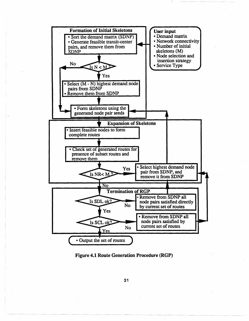
Formation of Initial Skeletons ' User input ~
• Sort the demand matrix (SDNP) • Demand matrix • Generate feasible transit-center ...... • Network connectivity pairs, and remove them from -- • Number of initial SDNP skeletons (M)
-i • Node selection and
No insertion strategy
-- -JLN< • Service Type ..... ~
,Yes
• Select (M - N) highest demand node pairs from SDNP
• Remove them from SDNP
, It
, • Form skeletons using the
~ --generated node pair seeds -j~
t Expansion of Skeletons
• Insert feasible nodes to form complete routes
t • Check set of generated routes for
presence of subset routes and remove them
1 Yes • Select highest demand node
IsNR< - pair from SDNP, and r- .. ~ , remove it from SDNP -~
No Termination of RGP ....
• Remove from SDNP all -IsSDLok? node pairs satisfied directly -- No by current set of routes 1 Yes - • Remove from SDNP all
IsSCLo? - node pairs satisfied by --.. r-
lYes No current set of routes
( • Output thd set of routes )
Figure 4.1 Route Generation Procedure (RGP)
31
----I

Step 6 Check for overlapping routes, and eliminate them from BR.
Step 7 Check the number of routes (NR) in BR .
If NR ~ M, go to Step 9.
Step 8 Select the first node pair in the remaining SDNP as the next node pair seed, remove
it from the remaining SDNP, and go to Step 4.
Step 9 Check system directness level.
If lower than user-specified level, remove the demand pairs satisfied directly by the
current BR from the remaining SDNP, and go to Step 8.
Step 10 Check system coverage level.
If lower than user-specified level, remove demand node pairs satisfied within two
transfers by the current BR from the remaining SDNP, and go to Step 8.
Otherwise, stop and obtain the resulting set of bus routes (BR), each route in the
set containing a list of demand nodes.
INPUT INFORMATION
The RGP requires the same input information as Baaj and Mahmassani's RGA, as well as two
additional control parameters for the selection of alternative design features. The input can be
grouped into the following five categories :
1) Network: The number of bus transit nodes, the connectivity list, the shortest path list for
each node pair, the next shortest path list for high demand node pairs, the
number of initial skeletons (M), the set of transit centers, and the set of terminal
nodes. '
2) Frequencies: The maximum frequency allowed on any bus route. This is used to provide a
route capacity constraint for the expansion routines.
3) Demand: A demand matrix representing the demand between each node pair, the
minimum system directness level (the minimum percentage of the total demand
to be satisfied directly, defined as *dsdirmin* in the computer program), and the
minimum system coverage level (the minimum percentage of the total demand to
be satisfied within two transfers, defined as *dsmin* in the computer program).
4) Parameters: The network deSign parameter for the selection of network designs with or
without the transit center concept, the service parameter for the selection of
uncoordinated and coordinated service deSign, the vehicle size parameter for the
selection of the fixed vehicle size option and variable vehicle size option, the
transfer penalty per transfer expressed in equivalent minutes of in-vehicle travel
32

time. the bus seating capacity (assumed the same on all buses). the maximum
load factor allowed by the transit planner on any bus route. the node-sharing
factor (·nsf·) necessary to determine whether a node can be inserted or not (see
discussion in section 4.5.2.2). and transferring flow factor necessary to determine
whether a route can be further expanded (see discussion in section 4.5.3.1).
5) Node Insertion Rules: Four node selection and insertion heuristics to be selected for route
expansion. including Maximum demand insertion (MD). Maximum demand per
minimum time insertion (MDMT). Maximum demand per minimum route length
increase insertion (MDMl). and Maximum demand per minimum cost insertion
(MOMe).
Table 4.1 summarizes the above input information and associated parameters and default values
used in the computer program.
FORMATION OF INITIAL SKELETONS
This step consists of two components. namely. the selection of initial node pair seeds and
the construction of initial skeletons from initial node pair seeds. These two components are
described in turn hereafter.
Selection of Initial Node Pair Seeds
The RGP starts by sorting the given demand matrix elements into a list of sorted demand
node pairs (SDNP) in decreasing order of demand. Then the RGP checks the set of transit
centers. *transit-centers·. 10r existence of any such center. If more than one center is specified,
the RGP calls for the predicate "feasible-transit-center-pairs" to determine the set of feasible
center pairs such that the travel time along the shortest path between each pair is less than a
preset maximum (currently 20 minutes). This maximum travel time reflects a feasibility guideline for
providing coordinated bus service between centers. Scheider and Smith (1981) suggested that
this time should be no greater than 20 minutes. The feasible center node pairs form seeds for
initial skeletons. The list of sorted demand node pairs is updated by eliminating all feasible transit
center pairs.
In the data input stage. the user is queried for the minimum possible number of routes (M)
required for the project area. If the number of feasible transit center pairs (N) is less than M, the
first (M - N) elements in the remaining sorted list of demand node pairs become skeleton seeds.
These elements are then removed from the updated list of sorted demand node pairs.
33

Table 4.1 Summary of Required Input Information for the RGP
Categories Parameters Definition VakJe
Network "connectivity-Iist* List of street network connectivity "asp" List of shortest path for each
demand node pair "aspk" List of alternate short paths "M" Number of initial skeletons . 1 "transit-centers" Set of transit centers nil "terminal-nodes" Set of terminal nodes nil
Frequency "max-frequency" Maximum allowed frequency
Demand "demand-matrix" Demand matrix representing the demand between each node pair
"dsdirmin" Minimum system directness level "dsmin* Minimum system coverage level
Parameters "tc-network?" Network constructed without transit center concept
Network constructed with transit center concept
"coordinated?" Design with uncoordinated service Design with coordinated service
*bus-size-option* Fixed vehicle size option variable vetOOle size option
*transfer-penalty* Transfer penalty expressed in equivalent of in-vehicle travel time
"seating-capacity" Bus seating capacity *max-Ioad-factor* Maximum load factor "nsf* Node-sharing factor "tran-flow-factor* Transferring flow factor
Node Insertion rules
*sra" Maximum demand insertion (MD) Maximum demand per minimum time insertion (MDMT)
Maximum demand per minimum route length increase insertion (MDML)
Maximum demand per minimum cost insertion (MDMC)
34
30 bus/hr
1
2 1 2 1 2
5· minutes 40 seats
1.25 0.75 0.25
1
2
3
4

The selection of the value M depends on the designer's knowledge of the service area.
However, if the designer's knowledge is poor or unreliable, the designer may examine data
pertaining to existing transit networks of cities in which the service population and trip patterns are
comparable to that of. the service area. Thus, it would be desirable to compile a data bank of
existing networks which can be consulted for the value of M. Alternatively, one can simply set M =
1 and let the RGP generate routes one by one.
Although the current version of the RGP selects feasible transit center pairs and high
demand node pairs as seeds for route skeletons; other alternatives may also be implemented if
the designer has sufficient knowledge of the network. First, the designer could specify as seeds
for route skeletons those demand node pairs identified as dominant trip generators and attractors.
Furthermore, the designer could also specify initial skeletons or routes directly if major corridors
are identified.
Construction of Initial Skeletons From Initial Node Pair Seeds
Each node pair seed forms a route skeleton along either its shortest path or an alternate path
connecting the corresponding node pair. The alternate path has a nodal composition
substantially different from that of the shortest path with a travel time that does not exceed the
shortest path by a given circuity factor. This factor is taken as 50% for high demand node pairs
and 25% for feasible transit center pairs to ensure more direct service between transit centers. A
path has significantly different nodal composition from that of a path P if the number of common
links contained in both paths does not exceed a ratio (say 50 %) of the total number of links of
path P. ,
The label-setting shortest path algorithm developed by Dijkstra (1959) is applied to generate
the shortest path for all node pairs in the transit network. The label-setting k-shortest paths
algorithm (Shier, 1979) is utilized to generate up to the 10th shortest path between any node pair
seed. Any path longer than the 10th shortest path is expected to violate the in-vehicle travel time
constraint. Thus, the shortest path for each node pair seed is defined. and the remaining nine
paths (sorted in increasing order of in-vehicle travel time) are examined sequentially to find an
alternate short path which meets three criteria: 1) it should not contain cycles, 2) its in-vehicle
travel time meets the circuity limitation, and 3) the number of common links shared with the
shortest path does not exceed 50% of the total number of shortest path links. If such a path is
found for the node pair. it is assigned as an alternate path. Otherwise, the skeleton is constructed
along the shortest path of the node pair. Both algOrithms were implemented by Baaj (1990).
As indicated by Baaj (1990). a skeleton along the shortest path of a high demand node pair
35
reduces its contribution to the total in-vehicle travel time to the minimum value but would likely
have fewer nodes than longer paths. However, if the skeleton is constructed along an alternate
short path comprising more nodes, it may satisfy a higher share of the total demand with only a
small Increase in the total trip time. Therefore, it is desirable to investigate both types of
skeletons. Baaj used a typical case to examine the resulting networks, and concluded that if
shortest paths are used in the procedure instead of alternate short paths, fewer buses are
required, but higher total user traveltime is incurred.
EXPANSION OF SKELETONS TO ROUTES
In this section, the procedure that expands skeletons to complete routes is discussed. This
procedure starts by finding the set of candidate nodes for insertion into a route under expansion.
Candidate nodes are inserted in the current route one at a time. The order of insertion follows a
certain sorted property, described in Section 4.5.2.5. In addition, each candidate node should
satisfy both the route capacity and length constraints .after expansion. The procedure terminates
if no candidate node is available for insertion.
The following criteria are utilized to check each node for insertion feasibility:
1) the resulting route does not form a loop after inserting the node (see Section 4.5.2.1
for more detail),
2) the node still has a low percentage of its total originating demand satisfied directly after
previous insertions in other routes (discussed in Section 4.5.2.2),
3) the resulting route does not become circuitous (discussion in Section 4.5.2.3), and
4) the ratio of the contributed demand satisfied per insertion cost (in-vehicle travel time)
exceeds a preset desired level (explained in greater detail in Section 4.5.2.4).
For nodes specified as transit centers, criterion 2 is relaxed since a large number of
transferring trips is expected at these centers. Therefore, more routes could be routed through
transit centers so as to increase accessibility and transfer opportunities.
Once the set of candidate insertion nodes is defined, the order of insertion depends on the
ratio of the contributed demand satisfied to the insertion cost. The intent is to insert the node with
the highest contributed demand satisfied per insertion cost into the route under expansion.
Transit centers are inserted with priority because of the expected large number of transferring
trips. In other words, if transit centers are contained in the set of candidate insertion nodes, the
insertion procedure considers these centers first, and then other candidate insertion nodes
(discussed in Section 4.5.2.4). Two constraints are checked before inserting a node:
1) the required service frequency on the resulting route does not exceed the maximum
36

operationally implementable value (default 30 buses/hour), and
2) the round trip time of the resulting route does not exceed a maximum allowable value
(default 2 hours, suggested by NCHRP 69).
If a candidate node satisfies both constraints, it is inserted into the route under expansion.
Otherwise, the route is complete, and the RGP expands the remaining skeletons. Figure 4.2
shows the flow chart of the route expansion procedure, including all the above insertion feasibility
checks.
Order of Expansion
Once M skeletons have been generated, the RGP expands them sequentially to form M
routes. The order of expansion determines the nodal compositions of the set of final routes for
the following two reasons:
1) Some nodes previously inserted into other routes may not be available for insertion
into the current route because most of their originating demand has been satisfied
directly (see insertion criterion 2) .
2) If a node is inserted into a high or a low demand node seed, it will result in different
contributions to the total in-vehicle travel time, and the sequence of insertion within the
set of candidate insertion nodes will be altered. In other words, a node in the set of
candidate insertion nodes for a low demand node seed will have higher priority for
insertion than that of a high demand node seed.
For M skeletons, there are at most M! different expansion sequences. The procedure
considers only two extreme cases, namely in order of decreasing demand of the seed node pairs,
or in order of increasing demand. These cases have the potential to produce the most different
sets of routes, with respect to the performance indicators.
Selection and Insertion of Feasible Nodes
The procedure utilizes five criteria to obtain a feasible set of candidate nodes for insertion.
These criteria are route-looping, node-sharing, terminal node, route circuity, and order of
insertion. The node-sharing test .Is not applied to transit centers because a large number of
transferring trips is expected at these centers. In order to obtain good quality of service between
transit centers, a lower circuity factor is used for skeletons generated using feasible transit center
pair seeds. Among all candidate nodes, transit centers receive priority for insertion.
37
-- -----------~-
I

--.... ·Generate neighboring nodes
Route-Looping Test
Node-Sharing Test
Terminal Node Test
Route Circuity Test
Sorting Property Test
yes
·Select the fIrst node in SPL ·Remove the node from SPL
• Insert the node ..... 1--1 .Ex and the new route
SPL: a list of candidate nodes sorted in decreasing order of the sorting property.. .
RCC:Route capacity constramt RLC: Route length constraint
Terminate Route Expansion
Figure 4.2 Route Expansion Procedure
38
Route-Looping Test: In order to reduce the search space, the procedure checks only
neighboring nodes connected via a single link to any node of the current route rather than all
nodes in the network. Each neighboring node is then checked to see whether it already belongs
to the route under expansion, in which case it is removed from the candidate list to avoid loops.
Node-Sharing Test: The remaining list of neighboring nodes is then checked to remove
nodes that have a high percentage of their total originating demand already satisfied directly. This
check is via a node-sharing factor (*nsf*, currently set at 75%) that determines when a node is no
longer available for insertion into routes under expansion. Therefore, once the percentage of
directly satisfied demand of any node in the remaining list is greater than * nsf* , it is removed from
the list. This criterion is based on the following ideas:
1) A node can be traversed by several routes, so insertion in one route does not preclude
insertion in skeletons expanded later. As more routes traverse this node, more of the
node's originating demand is satisfied. However, any further increase in the number of
traversing routes will not contribute much more to the demand satisfied directly.
2) In a transit network, passenger trips can be completed either directly or by transfers.
Demand originating at a given node that cannot be completed directly could be
completed via transfers. Inserting nodes with much of the originating demand already
satisfied directly will not be economical.
3) From the computational point of view, it would be burdensome to keep track of the
demand originating at a given node that would be satisfied via new transfer , opportunities as routes are expanded later in the process. The RGP keeps track only of
the demand originating at a given node that can be satisfied directly.
The remaining list is then filtered via a terminal node test.
Tennlnal Node Test: The default set of terminal nodes is an empty set unless specified
otherwise by the designer at the input stage. If this set is not empty, the end nodes of the current
route are checked for membership in this set. The procedure then removes from the remaining
candidate list all nodes for which insertion is via a connection to an end terminal node.
Route CircuIty Test: Transit routes should be direct and avoid circuitous paths. Each
candidate node that passes the previous three tests is examined under the route Circuity test for
insertion feasibility. This test compares the end to end trip time of the resulting route to the
shortest trip time between those end nodes. If the trip time ratio of the resulting route exceeds a
39

preset circuity factor (currently set to 1.50 for a/l routes expanded from high demand node pair
seeds and 1.25 for all routes expanded from feasible transit center node pair seeds), then the
node being tested is dropped from the list. This test checks all nodes remaining in the list for
circuity and generates a new candidate list.
Order of Node Insertion and Sorting Properties for Insertion: The previous
screening tests generate a set of candidate nodes for insertion. The order of inserting these
nodes affects·not only the nodal composition of the route under expansion but also that of routes
to be expanded later. Baaj (1990) has suggested that the order of expansion follow one of the
following four sorting properties based on the cost and/or benefits to the user and/or the
operator:
1) direct demand satisfied as a result of inserting the candidate node; this sorting property
considers only user benefits without regard to cost.
2) direct demand satisfied per increase of the total in-vehicle travel time as a result of the
insertion; this reflects the marginal user benefits relative to the marginal user cost.
3) direct demand satisfied per increase in round trip time of the route under expansion as
a result of the insertion; this reflects user benefits versus operator costs.
4) direct demand satisfied per increase of the sum of the total in'-vehicle travel time and
the round trip time; this measures the user benefits versus the sum of the user cost and
. operator cost.
Baaj developed a specific node selection and insertion strategy associated with each sorting ,
property, namely, Maximum Demand Insertion (MD), Maximum Demand per Minimum Time
Insertion (MDMT), Maximum Demand per Minimum Route Length Increase Insertion (MDML). and
Maximum Demand per Minimum Cost Insertion (MDMC), respectively. All four strategies are
implemented in the RGP. The details of these strategies are discussed in Appendix A.
At the program input stage, the designer is queried to specify the selection and insertion
strategy for each design execution. Candidate nodes with a sorting property value less than a pre
specified value (defined for each of the four sorting properties) are discarded. The remaining
candidate nodes are divided into two groups. The first group consists of all transit center nodes.
The remaining candidate nodes form the second group. Each of the two groups is sorted in
decreasing order of the sorting property value. The insertion procedure checks the transit center
candidate list first, followed by the second list. until a feasible node is found which satisfies both
route capacity constraint (discussed in section 4.5.3.1) and route length constraint (discussed in
section 4.5.3.2). This feasible candidate node is inserted and the resulting new route becomes a
40

candidate for further expansion. If no feasible node in the candidate list can be found, the
expansion process for the route terminates and the next skeleton is selected for expansion.
Termination of Route Expansion
The route expansion procedure terminates if no node in the candidate list satisfies either the
route capacity constraint or the route length constraint. These two constraints are described
hereafter.
Route Capacity Constraint: The route capacity constraint is based on the idea that if
the route service frequency exceeds a maximum implementable level (30 bus/hour) then the
schedules will be difficult to maintain. Before a node is inserted, the maximum link flow (Qmax) for
the route after inserting the node is compared to the allowable maximum link flow capacity
(LFCmax). If Omax is greater than LFCmax, the node is removed from the candidate list for
insertion. LFCmax is the product of the maximum allowable load factor on buses, LFmax; the
maximum implementable frequency, fmax; and the bus seating capacity. CAP. This can be
expressed as:
LFCmax = LFmaxfmaxCAP (4.5.1 )
Since it is too cumbersome to keep track of all link flows for each route under expansion, the
RGP approximates the maximum link flow (Omax) for the route under expansion by multiplying the
route's directly satisfied flow, OF, (i.e. corresponding to node pair demands that are satisfied
directly by the route) with the following factors:
1) (1 +ftf). ftf is the transferring flow factor (currently set at 0.25) which accounts for the
transferring flow on the route.
2) flf, maximum link flow fraction. The RGP uses the middle link's flow as the estimate of
the route's maximum link flow if the number of nodes (n) of the route under expansion is
even. If n is odd, the same fraction as for the case with n+1 nodes is used in the
computation. In order JO obtain the fraction, the same amount of originating demand is
assumed for each node on the bus route except for terminating nodes which have zero
originating demand. Therefore, all non-terminating nodes carry 1/(n-1) of the total
demand for cases with an even number of nodes and 11n of the total demand for cases
with an odd number of nodes. It is also assumed that all the originating demand
upstream of the middle link on each bus route will traverse the middle link. Therefore,
the fraction, flf, is computed as follows:
41
----- ---- ---- ----- --"- ----------------------- --- - ---- ---------1 -----~ "----- - - ----- --- ---

f _ n If - 2(n -1)
ifn is even
(4.5.2)
(n +1) = ifn is odd
2n
where n is the number of nodes of the route under expansion.
The same formulation is used by Baaj to estimate the maximum link flow fraction. The
approximate maximum link flow is then given by following equation:
Qmax = (1+ftf)fJfDF (4.5.3)
Route Length Constraint: As recommended by NCHRP 69 (1980), excessively long
routes should be avoided because bus schedules for long routes are difficult to maintain. In
general, the route length should not exceed two hours per round trip. The RGP checks each
candidate node for insertion to see if it violates the route length constraint.
SUMMARY OF RGP FEATURES
For the purpose of this study, the RGP needs to generate quality bus route networks that
allow the deSigner to implement ahernative design concepts. The RGP achieves this requirement
by providing the following important features:
1) It constructs route networks that incorporate the transit center concept. The RGP selects
feasible transit center pairs as seeds for constructing initial skeletons; it also uses a lower circuity
factor while generating routes between transit centers. These actions resuh in more direct service
between transit centers. In the route expansion step, transit centers are inserted with a higher
priority. This action resuhs in more routes available at the transit centers, and thus increases
accessibility and transfer opportunities at the centers. In addition, after the desired level of system
directness is satisfied, routes are constructed so that the remaining unsatiSfied demand (usually
dispersed) can be satisfied through the closest feasible transit center to reduce unnecessary
vehicle miles. As a result, the resulting route networks from the RGP are suitable for the· provision
of timed-transfer service and will support the implementation of demand responsive service as
well.
2) It is heavily guided by the demand matrix. This can be seen in the selection of node pair
seeds. The RGPselects high demand node pairs to form route skeletons. As a result, the
generated bus routes directly serve large portions of the total demand.
3) It constructs the routes along the shortest path or alternate short path of high demand
42
node pairs. This results in low user travel time cost and high system effectiveness.
4) It constructs different sets of routes corresponding to combinations of objectives. Guided
by the designer's specifications, the RGP generates sets of routes corresponding to different
system service directness levels, system coverage levels, and node selection and insertion
strategies (reflecting user and/or operator costs).
5) It incorporates necessary service planning guidelines including guidelines for route length
, route directness, route structure, and loop avoidance.
6) It allows the designer's knowledge to be implemented so as to possibly reduce the search
space. In the RGP, the following may be specified by the designers to possibly improve the
search efficiency: the minimum number of routes (M), order of expansion of the initial skeletons, -
the strategy for node selection and insertion, and identification of terminal nodes.
The route networks generated by the RGP are analyzed via the network analysis procedure
(NETAP). This procedure assigns known demand between origin-destination pairs to the transit
network, determines route frequencies and vehicle sizes (if the variable vehicle size option is
chosen), and computes a variety of performance measure. In the next chapter, the NETAP will be
presented along with an application to the transit data of Austin, Texas, which illustrates the RGP
and the NETAP. In addition, extensive tests of the RGP are presented in Chapter 7.
,
43
------ --- ---- -- ------r--- - - --- ------- --- -- - --

CHAPTER 5. THE NETWORK ANALYSIS PROCEDURE
INTRODUCTION
The network analysis procedure (NETAP) is intended for analysis and evaluation of
alternative network structures and service plans. For a given route configuration and service plan,
it computes a variety of system perlormance measures reflecting the quality of service and the
cost experienced by users. In addition, it determines the fleet size, operation cost, and fuel
consumption reflecting the resources required by the operator. As an analysis and evaluation
tool, the NETAP enables transit planners to evaluate existing or proposed systems.
The role of NETAP in the overall design procedure was described in Chapter 3 and illustrated
in Figure 3.1. For the purpose of this study, the NETAP determines route frequencies and
vehicle sizes for sets of routes generated by the RGP and evaluates the resulting system. It is
also used anytime perlormance measures for a given network configuration are desired, such as
following application of the network improvement procedure (NIP) to determine the extent of
improvement and/or worsening in the perlormance measures of interest.
The major NETAP features that differ from other approaches are the ability to analyze
coordinated bus systems and to determine coordinated bus route frequencies and variable
vehicle sizes. The NETAP uses a multiple path assignment model that explicitly accounts for trip
transfers at coordinated operation terminals. In addition, with minor modification, the model also
handles the trip assignment for integrated bus systems. The NETAP uses an iterative procedure
to achieve internal consistency of vehicle sizes and route frequencies. Route frequencies for , coordinated operation are obtained by adjusting the frequencies of routes that meet at the same
transit center to the same or multiple integer values after each iteration of the frequency setting
and vehicle sizing procedure.
In the next section, an overview of the NETAP and a summary of its steps are presented.
The required input information to execute the NETAP is presented in Section 5.3. Section 5.4
. discusses the trip assignment model and the computation of network descriptors. Section 5.5
presents the frequency setting and vehicle sizing procedure, including frequency adjustment for
coordinated operation. In Section 5.6, computation of system performance measures and
determination of network structure are discussed. The final section presents an illustrative
application using transit data from Austin, Texas. This application employs the RGP to generate a
route network around the transit center concept. The NETAP is then utilized to determine route
frequencies and vehicle sizes and to evaluate the resulting bus system.
44

OVERVIEW OF THE NET AP
Eight types of information are determined by the NETAP; these are:
1) Network descriptors consisting of the following three types of data:
• Node information contains originating flow, terminating flow and transferring flow at
each demand node. This information is used in the transit center selection procedure
(discussed in Section 6.3).
• Link information includes link flows along each route. The maximum link flow on each
route is used to determine route frequencies, optimal vehicle sizes, and maximum
load factor (discussed in greater detail in Section 5.5).
• Route information includes the round trip time for each route and the total number of
passengers on each route. This information is applied to compute the optimal vehicle
size. The round trip time is also used to obtain total vehicle miles and required fleet
size.
2) Demand: the total number of trips in the system as well as the percentages of demand
that are unsatisfied, or satisfied with 0, 1, or 2 transfers.
3) User cost: the total travel time experienced by users in the system, and the respective
percentages of in-vehicle travel time, waiting time, transfer time (reflecting a
prespecified time penalty considered to be equivalent to a transfer), equivalent in
vehicle-travel time cost, and equivalent waiting cost.
4) Level of service: the service frequency, vehicle size, and load factor associated with
each route.
" 5) Operator cost: the system operation cost and the required fleet size.
6) Fuel consumption: the total system fuel consumption.
7) System utilization: the ratio of the system actual user miles to the total user miles that
can be provided by the system.
8) Network structure: classification of network as one of four network shape categories,
namely, radial, spinal, grid, and delta networks. In addition, the network is classified as a
one-nucleus, two-nucleus, three-nucleus, or multiple-nucleus network.
This information provides the principal measures of system efficiency, service quality, user
cost, operator cost, and system utilization that are of interest in the evaluation of a particular transit
route network configuration and service plan.
The NETAP is a bus transit network evaluation tool. In this study, it is also used to determine
route frequencies and vehicle sizes. Once the RGP generates a set of routes, it is analyzed via
the NETAP to determine route frequencies and vehicle sizes (if the variable vehicle size design
45
------------- ------

option is selected); then the resulting system is evaluated. To accomplish these tasks. the
NET AP employs an iterative procedure that seeks to achieve internal consistency of frequencies
and vehicle sizes. This iterative procedure consists of two major components, namely, a trip
assignment model and a frequency setting and vehicle sizing procedure.
Since route frequencies are required before performing the trip assignment process, an
initial set of frequencies is assumed for each route when the NETAP is used for design purposes.
The NETAP then computes the round trip time of each route. Next, it utilizes the trip assignment
model to assign known demand between origin-destination pairs to the transit network so as to
obtain desired network descriptors. At the same time, a variety of performance measures with
respect to demand and user costs are computed.
The trip assignment model at core of the NETAP was developed by modifying Baajand
Mahmassani's (1990) TRUST procedure. This model first classifies all demand pairs into 0-
transfer, 1-transfer, 2-transfer, and unsatisfied (more than two transfers) demand pairs. System
performance measures pertaining to demand (system demand satisfied without transfer, with 1
transfer, with 2 transfers, and unsatisfied system demand) are computed at the same time. The
model then takes one node pair at a time and identifies the corresponding competing feasible
paths. The definition of competing paths for a certain node pair is based on a lexicographic
strategy that considers two criteria: 1) the number of transfers to reach the trip destination and 2)
the trip time incurred on the alternative paths. A tripmaker is assumed to always attempt to
complete his or her trip by following the path that involves the fewest possible number of
transfers. When several paths have the same (minimum) number of transfers, passengers are ,
assumed to use paths with travel times within a threshold (default 10%) of the least time path.
Trips for each demand pair are assigned to competing routes at the origin and further assigned at
transfer nodes if transfers are needed to complete the trip. Predicates "decide-O", "decide-1",
and "decide-2" with certain rules corresponding to the assignment of the O-transfer, 1-transfer,
and 2-transfer demand pair are performed. The demand split among competing paths is
computed according to certain rules that account for both uncoordinated and coordinated
operations (discussed in Section 5.4.2). Network descriptors and system performance measures
pertaining to user costs are updated when a given amount of demand is assigned to each
competing path. The trip assignment model sequentially considers each demand pair until all
demand pairs are assigned.
For integrated bus systems, the procedure ("drs-assign-demandH), is modified from the
above to assign and reallocate unsatisfied fixed service demand (after performing the above trip
asSignment procedure) to the transit network (discussed in greater detail in Section 5.4.5). The
46
role of wdrs-assign-demand" in the design of integrated bus systems is presented in detail in
Section 6.3.3 and illustrated in Figure 6.2.
Once the trip assignment procedure is complete, the resulting network descriptors are
applied to determine the vehicle size and route frequency for each bus route. The frequency
setting and vehicle sizing procedure computes the optimal vehicle size via a mathematical
formulation which minimizes the total cost (operator cost and user cost) of each individual route.
The total number of passenger trips, the maximum link volume, and the round trip time of a given
route, determined in the trip assignment procedure, are required to calculate the optimal vehicle
size. Once the vehicle size on each bus route is determined, the frequency of service is set to
achieve an applicable maximum allowed load factor. For timed-transfer design, the resulting
frequencies (set by the above definition) of routes that meet at the same transit center are
adjusted to the same or multiple integer values for coordinated operation. Then the resulting
route frequencies of service are compared to the input frequencies for each iteration. If
frequencies of two consecutive iterations converge, the NETAP calculates system performance
measures pertaining to operator cost, level of service, fuel consumption, and system utilization,
and determines the network structure. If the revised frequencies are significantly different from
the input values, the NETAP reiterates with the revised frequencies as the input frequencies.
However, H the NETAP is used for evaluation purposes only, the procedure for determining
service frequencies and vehicle sizes is skipped. The flow chart of the NET AP is shown in Figure
5.1. Section 5.5 describes in greater detail the frequency setting and vehicle sizing procedure.
In summary, the NETAP conSists of the following steps: ,
Step 0 If the NETAP is used for design purposes, set an initial frequency for eaCh bus .
route. Otherwise, go to Step 1.
Step 1 Compute round trip time for each bus route.
Step 2 Classify each demand pair into unsatisfied, O-transfer, 1-transfer, or 2-transfer
demand pair, and compute system demand measures for each category.
Step 3 Assign demand to the network.
3a Set i = O,j-O.
3b Assign the demand of node pair (i,j), NP(i,i), according to rules associated with
Its demand category, and update network descriptors and system performance
measures pertaining to user costs .
3c If j < N (the total number of demand nodes), set j = j + 1 and go to 3b.
3d If i < N, set i = i + 1, j = 0, and go to 3b.
Step 4 If the NETAP is used for design purposes, determine vehicle size and service
47
T- -
frequency for each route. Otherwise, go to Step 6.
Step 5 Check if two consecutive sets of route frequencies converge.
If not, set input route frequencies to the revised frequencies and go to Step 3.
Step 6 Compute system performance measures pertaining to operator cost, level of
service, fuel consumption, system utilization, and network structure.
INPUT INFORMATION
When the NETAP is employed as part of the overall design procedure, its input data include
part of the information supplied by the RGP and the following parameters: 1) a user specified
maximum number of iterations for the frequency setting process, 2) operator cost coefficients (a
and b, defined in Section 5.5.1) used in determining the optimal vehicle sizes, 3) the in-vehicle
travel time value (x) and the waiting time value (w), and 4) a set of pre specified available vehicle
sizes and the fuel efficiency coefficient (fi) associated with each vehicle size i.
If the NETAP is used independently as an evaluation tool for a given bus network, its input
data consists of the following four categories:
1) Network: the number of bus transit nodes, lists of nodes corresponding to each bus
route and the associated name of each route, a connectivity list , and a list of transit
centers.
2) Demand: a symmetric demand matrix representing the demand between each transit
node pair.
3) Service characteristics: the service frequency for each bus route, the vehicle seating
capacity for each'bus route, the allowable maximum load factor, and the vehicle operating
speed.
4) Parameters: the transfer time per transfer reflecting the penalty in equivalent minutes of
in-vehicle travel time, the in-vehicle travel time value (x), the waiting time value (w),
operator cost coefficients (a and b), and the fuel efficiency coefficient (fi) associated with
each vehicle size i.
TRIP ASSIGNMENT MODEL AND COMPUTATION OF NETWORK DESCRIPTORS
As mentioned in Section 5.2, the NETAP consists of two major components: the trip
assignment procedure and the frequency setting and vehicle sizing procedure. This section
focuses on the trip aSSignment procedure. For a given bus route network. and the associated
service frequency for each route, the trip aSSignment procedure assigns the demand of each
48

Decide-O • Assign NP (ij) demand • U date network descri tors
Decide-2 • Assign NP (ij) demand • U date network descri tors
No
No • Set frequencies .... __ .. ~ Fi=Fo
Figure 5.1 Network Analysis Procedure (NET AP)
49
,- ---- ---- --

node pair in the network (defined by a demand matrix) to the transit routes. Therefore, the transit
demand for each bus route in the network is computed and so is the flow on each link along the
bus route. The significance of the trip assignment to the analysis and design of transit networks is
demonstrated by three aspects: 1) the allocation of resources (vehicles) is highly dependent on
the amount of trips assigned to the transit network routes; 2) the evaluation of performance needs
accurate network flow information; and 3) the determination of route frequencies and vehicle
sizes requires demand information on both link and route levels.
The transit trip assignment problem differs from the auto trip assignment problem because of
waiting at transit stops or terminals. Due to the schedule variation for different available bus routes
to the trip destination, the decision of transit passengers may be affected by the availability and
the required waiting time of each available route. Many researchers have recognized these
phenomena, and developed multiple path assignment models. However, all previously
developed transit assignment models are limited to uncoordinated networks. In timed-transfer
systems, trip assignment becomes more complicated when several routes are coordinated to
arrive at a terminal within a preset time window.
As indicated by Speiss and Florian (1989), several authors have studied the transit trip
assignment problem in the past, either as a separate problem (Dial, 1967; Rapp et aI., 1976) or as
a sub-problem of more complex models, such as transit network design (Lampkin and Saalmans,
1967; Ma~le 1979; Hasselstrom, 1981), or multimodal network equilibrium (Florian and Speiss,
1983). Dial (1967) proposed a minimum weighted time path assignment, in which time spent on
different modes is differentially weighted. Lampkin and Saalmans (1967) assigned a fraction of ,
passengers to a route according to the probability that a vehicle serving this route arrives ea.rlier
than other routes. A lexicographic strategy, reflecting transfer avoidance andlor minimization as
the primary criterion for passenger route choice, was recommended by Han and Wilson (1982).
Their approach was motivated by systems with overlapping routes that have one or more links in
common. An optimal strategy (minimum generalized cost) assignment was presented by Speiss
and Florian (1989). In this model, a strategy is a set of rules for the selection of bus routes that
form a path to the traveler's destination. The optimization problem in this model was solved by a
label-setting algorithm. Baaj and Mahmassani (1990), in their Transit Route Analyst (TRUST).
adopted Han and Wilson's lexicographic strategy and Lampkin and Saalmans's "frequency-share
rule. In addition, they used a filtering process which applies a threshold check on the travel time to
eliminate any path with a trip time exceeding the minimum value among all possible paths by a
specified threshold.
As mentioned above, several transit trip assignment models have been developed to
50

support transit network design and analysis. These models are all limited to uncoordinated transit
networks. As many transit authorities have implemented timed-transfer transit systems, the need
for trip assignment models for coordinated transit systems is particularly important. In addition, for
the design of integrated bus systems described in this study, the trip aSSignment model should
also account for systems with combined fixed service routes and demand responsive service
routes. In this section, a more general model for uncoordinated, coordinated, and integrated
systems is presented. This model primarily builds on the trip assignment algorithm developed by
Baaj and Mahmassani's (1990).
Trip Assignment Characteristics In Timed· Transfer Systems
A timed-transfer transit system consists of coordinated routes in some or all transfer
terminals. These transfer terminals can be divided into 1) uncoordinated operations terminals, 2)
coordinated operations terminals with a common headway for all routes, and 3) coordinated
operations ter~nals with integer-ratio headways for all routes.
At uncoordinated operations terminals, vehicles are not scheduled to arrive simultaneously.
Transfer passengers usually need to wait for the next bus along the desired route to arrive. When
alternative routes are available and acceptable, transfer passengers may take the first bus to arrive
(among these routes) However, at coordinated operations terminals, all routes are coordinated to
arrive within the preset time window such that transfer passengers will not only have shorter
waiting times, but will also have a cluster of alternative routes to choose from.
Missed connections are a common occurrence at coordinated operations terminals. A " vehicle becomes unavailable if it arrives behind schedule. In other words, missed connections
reduce the set of vehicle routes available at a transit center, and may also cause trips to switch
from the missed route to other available routes.
Assignment Rules at Transfer Terminals
Different assignment rules need to be applied to reflect passenger route choice behavior
when trips involve different types of terminal operations. In our trip assignment model, the
-frequency-share- rule as described in Section 5.4 is used for uncoordinated operations
terminals. At coordinated operations terminals with a common headway, all competing routes are
available to transit passengers in all scheduled time windows. Therefore, a -least downstream
travel cost- rule which assigns all the demand to the route with the least downstream travel time is
utilized. Competing routes are those that pass a screening procedure, described later in Section
5.4.3. At coordinated operations terminals with integer-ratio headways, different combinations of
51
---~-
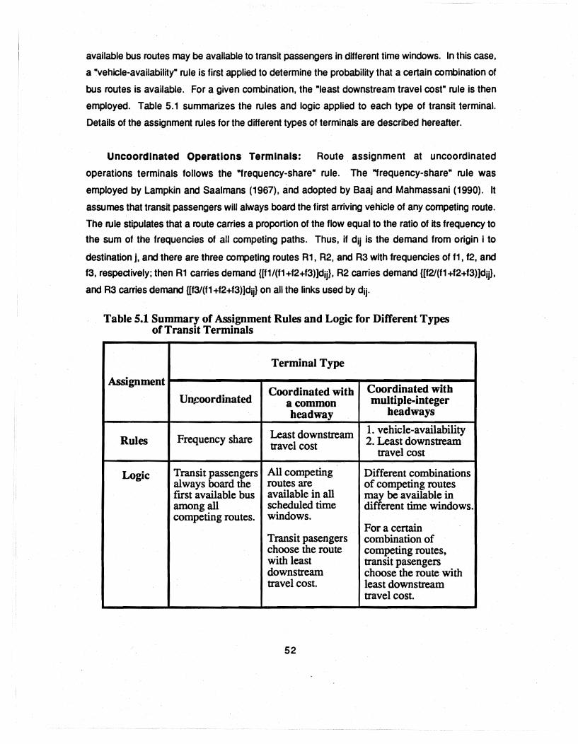
available bus routes may be available to transit passengers in different time windows. In this case,
a "vehicle-availability" rule is first applied to determine the probability that a certain combination of
bus routes is available. For a given combination, the "least downstream travel cost" rule is then
employed. Table 5.1 summarizes the rules and logic applied to each type of transit terminal.
Details of the assignment rules for the different types of terminals are described hereafter.
Uncoordinated Operations Terminals: Route assignment at uncoordinated
operations terminals follows the "frequency-share" rule. The "frequency-share" rule was
employed by Lampkin and Saalmans (1967), and adopted by Baaj and Mahmassani (1990). It
assumes that transit passengers will always board the first arriving vehicle of any competing route.
The rule stipulates that a route carries a proportion of the flow equal to the ratio of its frequency to
the sum of the frequencies of all competing paths. Thus, if djj is the demand from origin i to
destina.tion i, and there are three competing routes R1, R2, and R3 with frequencies of f1, 12, a.nd
f3, respectively; then R1 carries demand {[f1/(f1+f2+f3)]dij}, R2 carries demand {[f2/(f1+f2+f3)]dij},
and R3 carries demand {[f3/(f1 +f2+f3)]djj} on all the links used by djj.
Table 5.1 Summary of Assignment Rules and Logic for Different Types of Transit Terminals
Terminal Type
Assignment Coordinated with Coordinated with
UllS!oordinated a common multiple-integer headway headways
Frequency share Least downstream 1. vehicle-availability Rules travel cost 2. Least downstream
travel cost
Logic Transit passengers All competing Different combinations always board the routes are of competing routes first available bus available in all may be available in among all scheduled time different time windows. competing routes. windows.
For a certain Transit pasengers combination of choose the route competing routes, with least transit pasengers downstream choose the route with travel cost. least downstream
travel cost.
52

Coordinated Operations Terminals with a Common Headway: At coordinated
operations terminals, the "frequency-share" rule becomes Implausible because transit
passengers may have more than one route to choose from within the preset time window. In any
time window, it will be more appropriate to assign trips to the downstream route with the least travel
cost among available competing routes. In case of a common headway for all coordinated routes,
all competing routes will be available in all time windows. The "least downstream travel cost" rule is
applied on an "all-or-nothing" basis, with all trips (between a given 0-0 pair) aSSigned to the least
cost route.
Coordinated Operations Terminals with Integer-Ratio Headways: In the case of
coordinated routes with integer-ratio headways, some competing routes may be available at some
but not all time windows. In other words, different but still synchronized route frequencies result
in different combinations of simultaneously available bus routes for transferring passengers. For
example, consider two competing routes R1 and R2 with respective frequencies of one and two
vehicles per hour. R1 will be available only in alternate time windows, while R2 will be available in
all windows. In other words, one of every two consecutive time windows has both routes
available, while the other time window has only one available route R2. Therefore, to solve the
route aSSignment problem for coordinated operations terminals, a "vehicle-availability" rule is
applied to determine the probability Pi that passengers arrive at the terminal when a particular
combination of competing routes' vehicles Si'is available. The probability Pi is equal to the fraction
of the time windows which contain only the set Si. Within each set of competing routes defined in
the "vehicle-availability" rule, the "least downstream travel cost" rule is applied to assign demand
to the least travel cost downstream route.
To obtain Si and Pi. the following variables are defined:
fO is the frequency of route RO which carries flow into the coordinated operations terminal.
R1, R2, R3 .... Rn are competing routes at the coordinated operations terminal.
f1, f2. f3 ... , fn are route frequencies for competing routes R1, R2, R3 ... , and Rn,
respectively, with the relationship f1 ;;?: f2;;?: f3 ;;?: ... ;;?: fn,.
F - {fo, f 1, f2' f3 ... , fn} is the set of frequencies of all coordinated routes at the transfer
terminal.
Ai is equal to the ith minimum component of F, and Ao = O.
Si is the set of available competing routes with frequencies greater than or equal to Ai.
The total number of time windows available to passengers at a coordinated operations
terminal in a one-hour cycle is Min(fo, f1). The number of time windows containing any set of
53
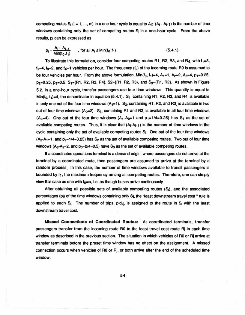
competing routes Si (i = 1, ... , m) in a one hour cycle is equal to Ai; (Aj - Aj-1) is the number of time
windows containing only the set of competing routes Sj in a one-hour cycle. From the above
results, Pi can be expressed as
A-A 1 p. - I I-
1- Min(fo,f,) , for all Aj ::;; Min(fo,f,) (5.4.1 )
To illustrate this formulation, consider four competing routes R1, R2, R3, and R4, with f,=8,
f~, f3=2, and f4=1 vehicles per hour. The frequency (fo) of the incoming route RO is assumed to
be four vehicles per hour. From the above fonnulation, Min(fo, f,)-4, A,=1, A2-2, A3=4, P1=O.25,
P2=O.25, P3=O.5, S,={R1, R2, R3, R4}, S2={R1, R2, R3}, and $a={R1, R2}. As shown in Figure
5.2, in a one-hour cycle, transfer passengers use four time windows. This quantity is equal to
Min(fo, f,)-4, the denominator in equation (5.4.1). S" containing R1, R2, R3, and R4, is available
in only one out of the four time windows (A,=1). S2, containing R1, R2, and R3, is available in two
out of four time windows (A2=2). S3, containing R1 and R2, is available in all four time windows
(A3=4). One out of the four time windows (A,-AO=1 and P1=1/4=O.25) has S, as the set of
available competing routes. Thus, it is clear that (Ai-Ai-1) is the number of time windows in the
cycle containing only the set of available competing routes Si. One out of the four time windows
(A2-A,.1, and P2=1/4=O.25) has S2 as the set of available competing routes. Two out of four time
windows (Aa-A2""2, and P3=214=O.5) have S3 as the set of available competing routes.
H a coordinated operations tenninal is a demand origin, where passengers do not arrive at the
tenninal by a coordinated route, then passengers are assumed to arrive at the terminal bya
random process. In this case, the number of time windows available to transit passengers is , bounded by f1, the maximum frequency among all competing routes. Therefore, one can Simply
view this case as one with fo=-, i.e. as though buses arrive continuously.
After obtaining all possible sets of available competing routes (Sj), and the associated
percentages (Pi) of the time windows containing only Si, the "least downstream travel cost" rule is
applied to each Sj. The number of trips, pjdjj, is assigned to the route in Sj with the least
downstream travelcost.
Missed Connections of Coordinated Routes: At coordinated terminals, transfer
passengers transfer from the incoming route RO to the least travel cost route Rj in each time
window as described in the previous section. The situation in which vehicles of RO or Rj arrive at
transfer terminals before the preset time window has no effect on the aSSignment. A missed
connection occurs when vehicles of RO or Rj, or both arrive after the end of the scheduled time
window.
54
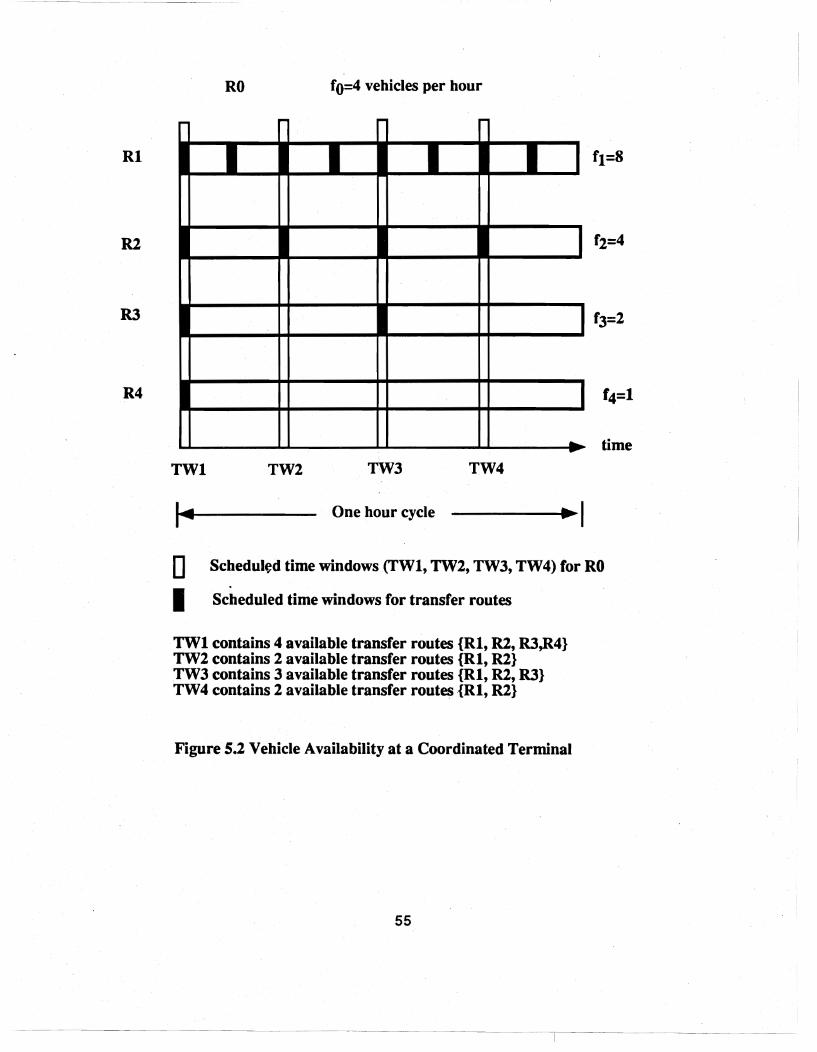
R1
Rl
R3
R4
RO fO=4 vehicles per hour
I"" I"" I"" I""
I I I I 1 I f1=8
I I
I I
I .. time
TW1 TW2 TW3 TW4
One hour cycle
o Scheduled time windows (TW1, TW2, TW3, TW4) for RO
I Scheduled time windows for transfer routes
TW1 contains 4 available transfer routes {R1, Rl, R3,R4} TW2 contains 2 available transfer routes {R1, R2} TW3 contains 3 available transfer routes {R1, R2, R3} TW4 contains 2 available transfer routes {R1, R2}
Figure 5.2 Vehicle Availability at a Coordinated Terminal
55
---- ---- ---r --- --- -

It is assumed that each coordinated route has the same probability of being late at all time
windows. In addition, unless this probability is quite high, it is unnecessary to account for
situations in which more than one coordinated route are late, since the joint probability of more
than one coordinated route being late will be very low and negligible. This model assumes that at
most one coordinated route may arrive behind schedule within each time window. Under these
assumptions, arrival of the incoming route RO behind schedule does not affect the trip
assignment, since for any time window there will be the same amount of demand due to this kind
of missed connection coming from the previous time window and going to the next window. For
the case that one of the outgoing routes is behind schedule, only the least travel time cost route
may result in assignment change if it is behind schedule. Under this situation, route assignment
needs to consider the following two cases:
Case 1 In time windows with more than one competing routes for transferring, the lost demand of
the least downstream travel cost route (due to the missed connection) will be shifted to
the route with the second least downstream travel cost.
Case 2 In any time window which has only one available route R1 (usually with the highest
frequency among all competing routes with integer-ratio headways), the lost demand of
R1, caused by its delay, is shifted to the route with the least downstream travel cost in the
next available time window. If the frequency of R1 (f1) is greater than the frequency of the
incoming route RO (fa). R1 must be the only available transferring route with frequency
greater than fa for the above case to occur. Under this condition, the "lost demand" of R1
reverts back to the same route but in the next available time window, where it will be the
only available rou(e. For cases with f1 £ fa, R1 may not be the only available route nor the
least downstream travel time route in the next available window. Furthermore. the next
available window may contain different combinations Sj (j = 1 •....• m) of available
competing routes. Each combination Sj contains routes with frequencies greater than
and equal to Aj, the jth minimum frequency of F as defined in the previous section.
Therefore, the fraction (rj) of the lost demand of R1 that shifts to the least travel time route
of a certain combination Sj needs to be defined. The fraction rj can be obtained as the
ratio of the number of "R1 only" windows followed by windows with Sj, to the number of
"R1 only" windows in a one hour cycle. Since f1 is the highest frequency among all
competing routes. Am is equal to f 1; Sm is the set of available competing routes with
frequencies greater than and equal to Am. In this case, 8m contains'only R1. The number
of "R1 only" time windows in a one hour cycle is equal to (Am-Am-1) as described in the
previous section. The number of "R1 only" windows followed by windows with 8j forj < m
56

in a one hour cycle is equal to (Aj-Aj-1). The number of "R1 only" windows followed by
windows with Sm (window containing only R1) in a one hour cycle is equal to (Am-2Am-1).
Therefore, ~ can be expressed as:
A·-A· 1 r. - J J-J-
Am -Am- 1
_ Am -2Am- 1
- Am-Am- 1
for j = 1, ... ,m-1, and
forj=m (5.4.2)
Thus, the previous model needs to be modified to reflect route assignment changes due to
missed connections; Pimc denotes the probability of being late for the route in the set of available
routes;-Sj (defined in Section 5.4.2.3), with the least downstream travel cost path. The
modification of the trip assignment procedure applies the following steps for each Sj.
Step 1 Check each Sj to see if it contains only one route R1.
If yes, go to Step 3.
Step 2 Assign PiPimc of the total trips to the route in Si with the second least downstream travel
cost, and Pi(1-Pimd of the total trips to the route in Si with the least downstream travel
cost.
Step 3 If f1 > fO, assign Pi Of the total trips to R1.
Otherwise,
(1) assign Pi(1-Pimd + PiPimcrm of the totaltrips to R1, and
(2) assign PiPimcrj of the total trips to the route in Sj (j = m-1, ... 1) with the least
downstream travel cost.
Trip Assignment Procedure for Timed-Transfer Systems
The trip assignment model presented here adopts the lexicographic strategy suggested by
Baaj and Mahmassani (1990), and incorporates the trip assignment concept for coordinated
operations terminals described in the previo~s section. In this model, all origin and destination
demand pairs are first classified as O-transfer, 1-transfer, 2-transfer, or unsatisfied (more than two
transfers) depending on the lowest number of transfers required for each demand pair. The
demand for each demand pair classified as O-transfer, 1-transfer, 2-transfer, or unsatisfied is
added to the following demand parameters *OEMANO-O-TRANSFER*, *OEMANO-1-
TRANSFER*, *OEMANO-2-TRANSFER*, and *UNSATISFIEO-OEMANO-LlST*, respectively.
These demand parameters are used later to compute the percentages of demand in the system
that are unsatisfied, or satisfied with 0,1, or 2 transfers.
57
-----r

When more than one paths have the same minimum number of transfers for a given demand
node pair, a "travel cost check" rule is employed to find a set of competing paths. This rule
eliminates paths with travel costs greater than a threshold above~ the minimum travel cost (from the
minimum travel cost path among aU paths with the fewest number of transfers). The assignment
for each demand node pair is based on the demand category (O-transfer, 1-transfer, and 2-
transfer) in which the node pair is classified. Assignment procedures applicable to each category
are applied. The demand of a given node pair is first assigned at the origin terminal, then
assigned at transfer terminals if necessary. Since three types of terminal operations need to be
considered In timed-transfer transit systems, the various assignment rules discussed in the
previous section are applied. The details of the trip assignment procedure for different demand
categories are described hereafter.
Classification of Demand Node Pairs: The trip assignment procedure for timed
transfer transit systems considers each demand node pair separately'. For a given pair, NP(i,j), 0-
transfer paths are searched for by checking the intersection of two sets of routes, SRo and SRd ,
which are the sets of routes passing through origin i and destination j, respectively. If the
intersection of SRo and SRd is not an empty set, the routes in the set are classified as O-transfer
paths for NP(i,j). A O-transfer path is denoted by a list (Ro, i, j) which represents passengers
boarding route Ro at the origin (i), and traveling on it to the destination (j). Once NP(i,j) is classified
as a O-transfer node pair, the parameter, *DEMAND-O-TRANSFER*, is then updated by adding
the demand dij of NP(i,j). Otherwise, there is no O-transfer path for NP(i,j), and the next level of ,
transfer paths (1-transfer paths) needs to be checked.
If djj cannot be assigned directly, paths that connect i and j with one transfer are searched for.
The search process for 1-transfer paths is carried out by examining the node lists of every
possible combination of route members of SRo (i.e., that pass through node i, say Ro) and of S~
(say ~), for the intersection set of nodes contained in both Ro and~. If the intersection set is not
empty, then its contents are possible transfer nodes for NP(i,j). For example, if the intersection
set contains (tn1, tn2 ... , tnk), there are k 1-transfer paths. Each of these 1-transfer paths is
denoted by a list «(Ro, i, tnkl(Rd, tnk, j))which represents passengers boarding route Ro at i, and
staying on it until node tnk, where the passengers transfer to route Rd, and travel on it until j. If the
demand node pair can be classified as1-transfer, *DEMAND-1-TRANSFER* is updated by adding
dij·
If no 1-transfer path can be found for dij (in the absence of O-transfer paths), then 2-transfer
paths are searched for. The process begins by finding a route, Re, that passes through neither
58

node i nor j, but shares a node with a route passing through i (e.g., Ro, a member of SAo) and
another node with a route passing through node j (e.g., Rd, a member of SRd)' The set of routes,
SRc, that passes through neither node i nor node j is the complement of the union of the
previously defined SRo and SRd, (SAo U SRd). For a trip to require exactly two transfers between
origin i and destination j, the first route Ro, has to pass through node i (hence, Ro CE SRo); the
second route Rc must be a member of SRc; and the third route Rd has to pass through node j
(hence, ~ CE SRd). Therefore, if the "list-of-nodes" of a route from SRc (say Rc) intersects both
the "list-of-nodes" of a route from SRo (say Ro), and the "list-of-nodes" of the route from SRd (say
Rd), then possible 2-transfer paths can be defined. A possible 2-transfer path is denoted by a list
with three components, ((Ro i tnl) (Rc tnl tnk> (Rd,tnk, j)). This list means that the passengers board
route Ro at i, and stay on it until node tn" where the passengers transfer to route Rc, and travel on
it until t"l<, where the passengers transfer to route Rd, and travel on it until j. If NP(i,j) can be
classified as 2-transfer, "OEMANO-2-TRANSFER" is updated by adding dij. Otherwise the
demand of the node pair is unsatisfied and is added to ".UNSATISFIEO-OEMANO-LiSr.
Assignment for o-Transfer Demand Pairs: For all the O-transfer paths, the 'ravel
cost check" rule is applied to eliminate O-transfer paths in which the travel cost exceeds the
minimum travel cost among all O-transfer paths by a specified threshold. In the current version of
NETAP, the travel cost function used in TRUST (Baaj and Mahmassani, 1990) is adapted. In this
function, the travel cost is equal to the sum of three components: total passenger waiting time,
total passenger in-vehicle travel time, and transfer penalties (5 minutes of equivalent in vehicle
travel time for each transfer). This cost function assumes the same value for each time
component. This assumption may be easily relaxed to account for different relative valuation of
different cost components.
The travel cost for a O-transfer path (Teo) includes the waiting time at the origin i (twait,i) and
the in-vehicle travel time from node i to node j using route Ro (tinvtt,ijIRo)' and can be expressed as:
TCo ... lmvtt,i jlRo + lwait,i
Since the given demand dij can be assigned without a transfer, assignment will only occur at
the origin node i. Thus, if node i is an uncoordinated operations terminal, the route assignment
rule for uncoordinated operations terminals should be applied. Otherwise, dij should be assigned
according to the rule for coordinated operations terminals. The downstream travel cost for a 0-
transfer path is equal to ~nvtt,ijIRo'
Assignment for 1-Transfer Demand Pairs: The same travel cost check process
described in the O-transfer case is applied to all 1-transfer paths to obtain the set of competing
59
-1----

paths. The travel cost for a i-transfer path, TC1 is computed as
TC1 = Iinvtt,i tnklAo + t;nvtt,tnk ilRcl + twait,i + tWait,tnk + tip
where
tip is the transfer penalty per transfer expressed in equivalent minutes of in-vehicle travel
time.
In the i-transfer case, trips are not only assigned at the origin, but also reallocated at the
transfer node. At the origin, the trip assignment procedure is the same as in the O-transfer case,
except that it is now applied to classes of paths rather than to individual paths. A class of paths is
formed by paths that share the same starting route (Ro) at origin. Demand is first allocated among
alternative classes; within each class, demand is then equally assigned to the constituent paths.
The fraction of demand that the whole class carries determines by using the assignment rules
described in Section 5.4.2, based on the terminal operation type of the origin. The downstream
travel cost at the origin for each path is equal to {tinvtt,i tnklRo + t;nvtt,tnk ilAd + twait,tnk + tip}.
Trips assigned to each path at the origin need to be reallocated at the transfer node, Paths
with the same starting route (Ro) and the same transfer node (tnlJ form a group Gok. Paths in each
group travel the same route from origin to the same transfer node, but use different routes to
travel from the transfer node to the destination. Based on the transfer node type, the total trips
assigned to each group are redistributed to the paths in the group using the appropriate route
assignment rule corresponding to the transfer node. The downstream travel cost for each
competing route at the transfer node is equal to ~nvtt,tnk iiAd'
Assignment for 2· T1'ansfer Demand Pairs: The same travel cost check is applied to
obtain the set of 2-transfer competing paths. The travel cost for a 2-transfer path, TC2 is
computed as
TC2 = finvtt,i tnklRo + ~nvtt,tnr tnklRc + lj"vtt,tnkiIRcl + twait,i + lwait,tnl + twait,tnk + 2t1p.
The trip assignment at the origin and at the first transfer node follows the same procedure as
in the i-transfer case, except that the downstream travel cost for paths at the origin is {TC2 -
twait,i}. and at the first transfer node is {tinvtt,tnl tnklRc + tinvtt,tnkilAd + tWait,tnk + ttp}. Similarly. at the
second transfer node, paths with the same upstream routes (Ro and Rc) and transfer nodes (tnl
and tnlJ form a group Goick. The sum of demand that each group carries after the assignment at
the first transfer node is then reassigned to the paths within that group at the second transfer
node using the appropriate route assignment rule. The downstream travel cost for each path at
the second transfer node is {~nV1t,tnkiIRcl}'
60

Underthe assumptions that 1) passengers arrive at random (uniformly), 2) passengers can
always board the first available bus, and 3) vehicles arrive at regular headways, the average waiting
time for passengers using a certain route is taken as half of the route's headway. This haH
headway assumption is used to compute the expected waiting time at trip origins and at
uncoordinated transfer terminates for the computation of travel time of competing paths. At the
trip origin, an average waiting time (in minutes) of 60.0/(210) (one haH Ro's headways) is used for
twait,i. At transfer terminals tnl and tnk, average waiting times (in minutes) of 60.0/(2fd), and
60.0/(2fd) (one half Rc's and Rd'S headways, respectively) are assumed for tWait,tnl and !wait,tnk if
these transfer nodes are not coordinated operations terminals. Otherwise, twait,tnl and !wait,tnk are
assumed to be one haH the preset time window (default 5 minutes).
The expected transit passenger waiting time for a certain bus route in an actual system
depends on both the reliability of the bus schedule and the distribution of passenger arrival times.
Under the assumption of uniformly distributed random passenger arrivals at bus stops, the
average passenger waiting time increases as bus headways become less regular and as more
passengers arrive in average during longer intervals and fewer during shorter intervals (Osuna and
Newell, 1972; Larson and Odoni, 1981). However, passengers may not necessarily arrive at
random in all cases. Some transit users tend, to some extent, to coordinate their arrivals with
published schedules, if available, especially for routes with long headways. Bowman and
Turnquist (1981) have derived an expression for the expected wait time when the population of
users is a mixture of "scheduled timers" and "random arrivals", The resulting waiting time function
is highly system dependent, and should be calibrated for each system, possibly for each bus
route. However, the effect of schedule timing is to some extent offset by schedule unreliability,
making the one-haH-headway assumption an acceptable compromise. More important, from a
deSign standpoint, virtually all procedures use that assumption for three primary reasons. First,
schedule variability is not intended by design, and is usually a reduction target by system
operators. Secondly, while "schedule timers" may not incur an actual physical wait time at the
stop, they incur a schedule delay relative to the actual time they would have wanted to depart.
From a user cost standpoint in a design procedure, it is this schedule delay cost that must be
included in the objective function, and not the actual time at the stop. Evaluating waiting time on
the assumption that users time their arrivals to coincide with the schedule can seriously
underestimate user costs and lead to deSigns that do not meet user needs.
Numerical Appllcatlon to a Single Demand Node Pair
To illustrate the assignment procedure described in th~ previous section, Figure 5.3 shows a
61

demand node pair (i,j) served by seven routes. Four examples are considered: 1) an
uncoordinated network; 2) a fully coordinated network with integer-ratio headways; 3)a fully
coordinated network with a common headway; and 4) a fully coordinated network with integer-ratio
headways and a probability of being late p=0.1 for all routes. Link travel times are shown in Table
5.2. Examples 1, 2, and 4 use the same route frequencies, also given in Table 5.2. A five minute
time window is used in aU the coordinated operations examples. The threshold for the travel cost
check is set at 10%. A five minute penalty per transfer is given for all cases.
Figure 5.3 Example Route Network with Six I-Transfer Paths
62

Table 5.2 Link Travel Times (minutes) and Route Frequencies (buses/hour) for Example of Figure 5.3
Links Ll L2 L3 L4 L5 L6 L7 L8 L9
Travel Times 8 4 5 6 9 8 8 7 8
Routes Rl Rl R3 R4 R5 R6 R7
Frequencies 8 4 4 2 4 4 2
Table 5.3 Path Links and Path Travel Cost for Example of Figure 5.3
Path List Representation Links Travel Cost (minutes) Uncoordinated Coordinated Downstream
PI «Rl i tnl)(R3 tn1 j» Ll,L6 31.8 26 8
P2 «Rl i tnl)(R2 tnl j» Ll, L3,IA 34.8 29· 11
P3 «R1 i tnl)(R4 tn1 j» L1,L5 40.5· 27 9
P4 «R1 i tnl)(Rl tn2 j» L1, L2,IA 33.8 28· 6
P5 «R5 i tn3)(R6 tn3 j» L7,L8 35 25 7
P6 «R5 i tn3)(R7 tn3 j» L7,L9 43.5· 26 8
• Paths eliminated by the travel cost screening process.
No O-transfer route can be found in the given network. Six 1-transfer paths are found in the
path search process. The link components for each path are presented in Table 5.3. The path
travel costs for both uncoordinated and coordinated operations· and the downstream travel cost at
the transfer node for coordinated operations are shown in Table 5.3 as well. After the travel cost
screening process, paths P3 and P6, and paths P2 and P4 are eliminated from the set of 1-
transfer paths in the uncoordinated and coordinated examples, respectively.
63
1- -- -~--- -- --

Table 5.4 Proportions of Demand Between Nodes iand j Assigned to Paths in All Cases
Paths PI P2 P3
At origin 0.22 0.22 O· Uncoordinated
0.22 0.22 O· Final assignment
At origin 0.25 O· 0.25 Coordinated
0.5 o· 0 Final assignment
At origin 0 O· 0 Common Headway
0 O· 0 Final assignment
At origin 0.25 O· 0.25 Missed Connection
0.475 O· 0.025 Final assignment
• Paths eliminated by the travel cost screening process.
Table 5.5 Proportions of Demand Between Nodes i and j Assigned to Links in All Cases
P4
0.22
0.22
O· O·
O·
o· O· o·
Links ,
LI L2 L3 L4 L5 L6 L7
P5 P6
0.33 O· 0.33 O·
0.25 0.25
0.5 0
0.5 0.5
I 0
0.25 0.25
0.5 0
L8 L9
Uncoordinated 0.67 0.22 0.22 0.44 0 0.22 0.33 0.33 0
Coordinated 0.5 0 0 0 0 0.5 0.5 0.5 0
Common Headway 0 0 0 0 0 0 I I 0
Missed Connection 0.5 0 0 0 0.025 0.475 0.5 0.5 0
Trip Assignment for Integrated Bus Systems
The trip assignment procedure presented in the previous sections handles both
uncoordinated and coordinated bus systems with fixed-route and fixed-schedule service.
However, the deSign of integrated bus systems is another alternative provided by the solution
framework. For this purpose, the trip assignment procedure should also account for systems that
combine fixed-route, fixed-schedule service with demand responsive service (DRS).
64

The integrated system consists of two sets of routes: fixed service routes and DRS routes.
Each route of both sets consists of a list of nodes. As assumed for the fixed-route, fixed
schedule system, passengers will be willing to travel by bus if their trips can be completed within
two transfers. Passengers in an integrated system are assumed to first consider the fixed route
service if their trips can be completed by such service. If not feasible, passengers then consider
using the demand responsive service or a combination of DRS and fixed route service.
Therefore, trip assignment for integrated bus systems first employs the assignment procedure
described in the previous sections for fixed route service to assign demand and identify demand
node pairs with unsatisfied passengers (by the fixed route service). Then, a modified procedure
is used to allocate and assign this unsatisfied demand to the integrated systems.
The modified trip assignment procedure distributes the demand unsatisfied by the fixed
route system to service segments in the integrated system. For example, consider a node pair (i,
j) with unsatisfied demand, dij' and served by two service segments, (DRSk i tn1) and (Rn tn1 j),
meaning that passengers board a DRS route at node i and stay on it until node tn1 where they
transfer to a fixed route and travel on it until node j. In the segments served by DRS routes, the
demand is satisfied by the DRS route k and thus the demand for route k is increased by an amount
dij. In the fixed route segments, the demand dij is added to the demand between node pair (tn1 ,
j) in the demand matrix. Furthermore, the demand of (i, j) is set to zero in the demand matrix. By
doing this, the demand previously unsatisfied in the fixed route system can be redistributed to the
fixed route network in the integrated bus system. After all the unsatisfied demand is reallocated, a
new demand matrix results. This demand matrix will be used to determine the flow distribution of
the fixed route service sO that the service frequency and vehicle size can be set for each fixed
route in the integrated bus system. In other words, a new demand matrix is used to run the fixed
route trip assignment procedure.
In a DRS service area, passengers unsatisfied by the fixed route can be delivered from or to
the transit center. A passenger whose destination or origin is covered by the DRS service area
needs to transfer at the transit center and then use the fixed route service or other DRS to
complete his or her trip. Therefore, fixed route unsatisfied passengers can be classified as drs-O
transfer, drs-1-transfer, drs-2-transfer, and drs-unsatisfied.
The trip assignment procedure considers each node pair with unsatisfied demand by the
fixed route system separately. For a given node pair (i, j) with unsatisfied demand, dij, drs-O-
transfer paths are searched for first by using the same procedure as described in Section 5.4.3.1
for O-transfer paths in the fixed route service system. If dij can be completed without transfer, it
must be served by at least one DRS route. Once a drs-O-transferpath (DRSk, i, j) can be found, dij
65
---- --------- - -I - ---,

is added to the demand of DRS route k. If more than one drs-O-transfer path is identified, dij is
equally assigned to each DRS route. No adjustment to the demand matrix is needed because
there is no fixed route service segment for the unsatisfied demand in this category. The demand
satisfied with 0 transfer (*DEMAND-O-TRANSFER*) is updated by adding dij.
H dij cannot be assigned directly, drs-1-transfer paths are searched for. The search process
for drs-1-transfer paths is similar to the process for 1-transfer paths in the fixed route service
system, as described in Section 5.4.3.1, except that passengers using DRS routes can only
transfer at transit centers and not at every node along the DRS route. Therefore, for any DRS
route considered in the search process, only the transit center is included in the "Iist-of-nodes" for
transferring (instead of the complete "list-of-nodes" of the route). A drs-1-transfer path can be
composed of either two DRS routes,{(DRSki tn1) (DRSI tn1 j)}, or a DRS route and a fixed route,
{(DRSk I tn1) (An tn1 j)}or {(Rn i tn1) (DRSk tn1 j)}. In the first case, dij is added to the demand of both
DRS routes. In the second case, both the demand of DRS route k and of node pair (tnd) (or node
pair(i tn1» are increased by djj. The demand of node pair (i, j) is set to zero. The demand satisfied
with 1 transfer (*DEMAND-1-TRANSFER*) is updated by addingdij. If more than one drs-1-
transfer path is found, passengers are assumed to choose the path with the fewest DRS
segments. Therefore, dij is equally assigned to each path with the fewest DRS segments.
H no drs-1-transfer path can be found for dij' the procedure that searches for drs-2 transfer
paths is invoked. The procedure is similar to the corresponding procedure in the fixed route
service system, with the modification that the DRS routes can only transfer at transit centers, as
described above for drs-1-transfer paths. There are two possible types of drs-2-transfer paths: ,
those with DRS routes at both ends of the path and a fixed route in the middle, and paths with two
adjacent fixed routes and one DRS route at either end of the path. The first type of path can be
denoted by a list {(DRSk i tn1) (Rn tn1 tnv (DRS! tn2 j)}. The second type can be denoted by {(DRSk
i tn1) (An tn1 tnv (Am t~ j)} or {(An i tn1) (Am tn1 t~ (DR~ tn2 j)}. H djj is satisfied by a path of the first
type, the demand of DRS routes k and route I, and the demand of node pair (tn1 tn2l are increased
by dij. For the second type of path, the demand of DRS route k is increased by dij. dij is added to
the demand of node pair (i tn2) if the path starts with a fixed route service. Otherwise, dij is added
to the demand of node pair (tn1 j). The demand of node pair (i,j) is set to zero, and *DEMAND-2-
TRANSFER* is updated by adding dij. If more than one drs-2-transfer path is found, the same
strategy as for the drs-1-transfer paths is applied. If no drs-2-transfer path can be found, the
demand node pair remains unsatisfied.
66
Computation of Network Descriptors
Through the property representation of the LISP computer language, node flows (consisting
of originating flow, terminating flow, and transferring flow). link flows associated with each route,
and route flow (total number of passengers served by the route) are initially set to zero. Link flow
values associated with a route are represented by a property list. For example, the link flows of R1
with nodal composition (0 1 2345) and R2 with nodal composition (45 678) are set to zero and
represented by the lists «1-0-1 0) (1-1-20) (1-2-30) (1-3-4 0) (1-4-50)) and «1-4-5 0) (1-5-60) (1-6-70) (1-
7-80)), respectively. Both R1 and R2 utilize the same physical link joining nodes 4 and 5, but for
the purpose of assignment and flow information, link 1-4-5 associated with R1 is different from link
1-4-5 associated with R2. After determining the competing paths and the associated percentages
of demand assigned to these paths for each demand node pair, the flow information for the node,
link, and route levels is updated by adding assigned demand to the proper nodes, links, and
routes that are traversed. For example, if p percent of dij is assigned via a 1-transfer path «R1 1 4)
(R2 4 7)), then the originating flow at node 1, the transferring flow at node 4, the terminating flow
at node 7, and the route flows forR1 and R2 are updated by adding the quantity of demand pdij.
In addition, the link flows of 1-0-1,1-1-2,1-2-3, and 1-3-4 on R1; and of 1-4-5,1-5-6, and 1-6-7 on R2
are increased by pdij.
FREQUENCY SETTING AND VEHICLE SIZING PROCEDURE
The previous sections presented the trip assignment procedure which computes network,
route, link, and node descriptors. When the NETAP is utilized as part of a design tool, it also calls
" a procedure to determine the service frequency and vehicle size for each bus route. This section
describes the iterative frequency setting and vehicle sizing procedure which yields internally
consistent service frequencies and vehicle sizes using information computed from the trip
assignment.
The well-known square-root rule for setting frequencies on bus routes is based on the
minimization of the sum of operator cost and passenger waiting time (Mohring, 1972). Major
weaknesses of the square-root formulation are that it does not account for bus capacity
constraints and that it assumes demand to be independent of service frequency. In the transit
industry, the frequency of service on a bus route is commonly set to achieve an applicable
maximum allowed load factor (Furth and Wilson, 1981), and can be written as:
fk = (Ok)max LFmaxVSk
where
67
(5.5.1)
-,---
fk is the route frequency for route k,
(00max is the maximum hourly link flow of route k,
LFmax is the maximum allowed load factor, and
VSk is the vehicle size (seats).
With this frequency formulation, transit operators can select the desired load factor so as to
meet operational considerations (such as comfort). Note that different load factors may be set for
different subsets of bus routes depending on the type of service provided, service area, and
other special considerations reflecting local political preferences. Of course, when the frequency
generated by this equation is unacceptably low because of low patronage, a minimum frequency
policy is commonly applied in practice.
Only in a few studies have vehicle sizes been computed explicitly. Glaister (1986)
developed a simulation model to compare system operations using two vehicle sizes, a large
vehicle (88 seats) and a small vehicle (15 seats). Results of the Simulation suggest that buses
seating 35 to 45 riders would likely be most suitable for service in Aberdeen. Its level of detail
notwithstanding, the computer simulation model does not explicitly describe the relationship
between bus size and factors such as level of demand, operator cost, and load factor. Analytic
models for finding optimal vehicle sizes have been developed for this purpose.
Previous analytic models include Jan~son's (1980), Walters' (1982), Oldfield and Sly's
(1988). and Chang's (1990). Jansson argued that previous analyses overweighed the producers'
costs and underestimated the users' cost. He presented a model that minimizes total social cost
including operator cost, passenger waiting time, and passenger riding time, subject to a peak
capacity constraint satisfYing a maximum occupancy rate (the ratio of the mean passenger flow to
the product of the vehicle size and the service frequency). Jansson concluded that the optimal
bus size determined by minimizing social cost tends to be smaller than the size used in current
practice, where vehicle size is given and the number of buses is determined so as to achieve an
average occupancy rate at or below a given maximum value. Walters presented a simpler model
that examines the trade-off between waiting time and labor cost. He also suggested that the bus
size should be considerably smaller than is typically used in cities of western Europe and North
America. Gwilliam et al. (1985) and Oldfield and Sly (1988) argued that the waiting time
assumption in Walters' model is questionable, and thus yields an implausible relationship between
optimal bus size and demand. Oldfield and Sly's model assumes elastic demand and determines
the optimal bus size by minimizing total social cost. In addition, the average passenger waiting
time in their model accounts for situations where passengers are unable to board the first bus to
arrive because it is full. They concluded that the optimal size lies between 55 and 65 seats (70-
68
seat buses are used by most existing systems in the United Kingdom). The current cost
structures could be changed to be more favorable to the operation of smaller buses, but the
optimal size seems unlikely to fall below 40 seats. Chang (1990) presented analytic models to
compare vehicle sizes between fixed route conventional bus and flexible route subscription bus
systems. He concluded that the optimal vehicle size for flexible route service is less sensitive to
the demand density than the optimal size for fixed route service.
All the previous analytic models focus on the optimization of vehicle size and frequency for
an individual bus route, which is treated independently of the other routes comprising the
network. In other words, the demand on a particular bus route will not be affected by the optimal
bus sizes and associated route frequencies of other bus routes. This is an incorrect assumption
because in a bus system, passengers may have several paths on which to complete their trips.
Changes to the bus size and route frequency alter the route level of service and should lead to a
redistribution of passenger flows on the bus network. Therefore, in designing route frequency
and vehicle size, the systemwide effects of changes in frequency and vehicle size need to be
considered.
Instead of assuming the demand on each bus route to be known and given as in all previous
models, the model presented here solves for the route demands by assigning the trips in a given
0-0 demand matrix using the transit trip assignment model described in Section 5.4. The transit
trip assignment model computes both the total passenger trips using route k (TPT k) and the
corresponding maximum link flow of route k, (Ok)max. The resulting maximumJink flow is more
reliable than the value obtained as the product of the maximum occupancy rate and vehicle
seating capacity. Both TPTk and (Ok)max then form the basis for obtaining a set of optimal bus
sizes (discussed in the next section) and the associated route frequencies (obtained by using
Equation 5.5.1) so as to minimize the generalized cost function. For timed-transfer system
design, the frequencies of coordinatad routes need to be set to the same or multiple integer
values. A frequency adjustment procedure is utilized to accomplish this task.
In determining vehicle sizes for different routes, itshould be kept in mind that it is not
practical to operate too many vehicle sizes in a system because of the resulting operational
complexity and associated maintenance costs. In the process for computing vehicle sizes
described above, a different vehicle size may be selected for each bus route and thus there will
be too many vehicle sizes to operate practically. To overcome this disadvantage, the procedure
allocates a set of pre specified vehicle sizes to each route using a simple nearest feasible integer
heuristic. Five different sizes of commercially available vehicles is an appropriate guideline for the
maximum number of vehicle sizes in a system. Shih and Mahmassani (1994) used an example
69
~-~- - - -- --~--- -- -_., -- ---,---- - ,----- -- ---
based on the data generated from Austin, Texas, transit system to show that meaningful benefit
can be observed even with a relatively small set of vehicle sizes.
An initial set of input frequencies is required for the trip assignment. The NETAP simply
assigns the same initial frequency of 10 buses/hour to all routes. Since the procedure changes
route frequencies from the input values to new values, the demand needs to be reassigned
consistently with the new frequencies, and the optimal vehicle sizes and route frequencies then
need to be recomputed as well. The procedure iteratively searches for internal consistency of the
route frequencies and vehicle sizes. In other words, this procedure continues until the revised
frequencies are not much different from the previous frequencies (up to 10 % deviation is
allowed).
The computation of route frequencies to achieve a preset peak load factor is only meaningful
when the demand assignment is performed over the peak hour period, especially if the network is
congested. However, one would expect the NETAP to be used for different time-of-day periods.
For less congested periods, the peak load factor may yield frequencies that are too low to be
reasonably expected by riders. In this case, minimum policy headways would be used. The
NETAP checks the output frequency for each route, which is computed to achieve the preset
-MAX-LOAD-FACTOR- (currently set to 1.25). If the frequency does not exceed a -CUTOFF
FREQUENCY· (currently set to 2 buses/hour), the route belongs to the category of low ridership
routes. The NETAP recomputes the frequency using a -MIN-LOAD-FACTOR· (currently set to
0.8) which represents the minimum load factor accepted by operators. If the recomputed
frequency is still less than a *MIN-FREQUENCY* (currently set to 1 buS/hour), then the output
frequency is set to 1 bus1hour, and the load factor is computed accordingly.
Optimal Vehicle Size for Single Route with Given Demand
The approach for determining the optimal vehicle Size for each individual route is similar to
the generalized cost approach used to obtain the square-root expression for frequency setting.
However, instead of considering the frequency as the decision variable and the vehicle size as a
constant, the vehicle size is taken as the decision variable, and the frequency is set as a function
of the vehicle size conSistently with equation (5.5.1).
For a given demand level on a bus route k, the optimal vehicle size is obtained by minimizing
the generalized cost (CiJ. which conSists of the operator cost (Cko) and the user cost (Cku); i.e. Ck
.. Cko + Cku. The derivation of the optimal vehicle size is based on peak hour operation, which is
the most critical period for determining the required system fleet size. However. the procedure
could be applied to any desired operating period.
70

Oldfield and Bly (1988) presented a reasonable and simple approximate formulation that
expresses total operator costs as a linear function of vehicle size, as follows:
~ = a (1 + b V$jJVMk (5.5.2)
where
a is a constant which adjusts the overall cost level,
b is a constant which captures the relative rate of increase in cost with increasing vehicle
size, and
VMk is the total vehicle miles per hour operated on route k.
The total vehicle miles per hour for each route k can be expressed as:
VMk = fk RTMk (5.5.3) -"
where
fk is the frequency of service on route k, and
RTMk is the round trip miles for route k.
Assuming that the function fk is set according to the equal peak hour load factor rule
(Equation 5.5.1), the operator's cost can thus be expressed as:
(0 ) C = a(1 + bS )RTM k max
ko k k LF VS max k
(5.5.4)
From the passengers' point of view, the total user cost (Cku) for route k consists of three
components: waiting cost (WCk), in-vehicle travel cost (IVTTCk), and access cost (ACk), as
proposed by Chang (1990).
(5.5.5)
Using the half headway assumption as described in Section 5.4.3.4, the average waiting time
for passengers using route k is taken as half of the route's headway. Assuming that waiting time is
valued linearly (an assumption which may be easily relaxed if alternative value functions are
calibrated from empirical behavioral data), the total waiting time for passengers using route k can
be expressed as:
1 LFmaxVSk WCk =wTPTk-=wTPTk---....
2fk 2(Ok )max (5.5.6)
where
w is the value of waiting time, and
TPT k is the total passenger trips (demand) per hour using route k (which is computed
in the trip assignment procedure).
The in-vehicle travel cost is assumed independent of vehicle size, primarily because in-
71

cost savings. In-vehicle travel cost reduction may arise mostly from possibly different average
vehicle speeds for different vehicle sizes. Smaller buses may provide faster service for two
reasons: 1) better maneuverability, and 2) fewer people getting on and off. On the other hand,
they may also increase traffic congestion since more buses will be operated on the road, and thus
the bus speed may decrease. Since bus speed is highly dependent on traffic conditions along
the route, any improvement in the in-vehicle travel time cost of smaller buses is usually limited and
insignificant relative to the potential waiting time cost saving. It should also be noted in this regard
that studies on the characterization of traffic service in urban street networks have strongly
suggested that the travel time and related service attributes experienced by vehicles of different
types over a sufficiently long period of time tend to be very similar because of the constraining
effect of traffic control and the character of urban traffic (Herman and Ardekani, 1984).
Another consideration for the constant IvnCk assumption is the difficulty and resulting
complexity of incorporating IVTTCk as a function of vehicle size in the cost function. The
relationship between vehicle speed and the vehicle size is difficult to specify analytically,
especially, in light of vehicle speed variation under different traffic conditions. Furthermore,
vehicles with the same size but different engines may have different acceleration and
deceleration characteristics. In light of the above, it seems hardly worth the effort to incorporate
route-dependent and condition-dependent IvnCk.
Using the above results and assumptions, the generalized cost Ck can be rewritten as:
(5.5.7) * Note that ACk and IVTTCk are independent of the vehicle Size. The optimal bus size VSk for
given route demand levels can be obtained by setting dCk/dVSk = 0, and can be expressed as:
VS~ = (Ok)max 2aRTMk (5.5.8) LFmax wTPTk
The relation. indicates that the optimal vehicle size for a given demand level on a route is proportional to the level of the maximum link flow «Oklmax)' and varies as the square root of round
trip miles of the route (RTMiJ. The optimal vehicle size is inversely proportional to the load factor
(LFmax), as well as the square root of the total number of passenger trips (TPT k) and the value of
waiting time (w).
In the above expression, the total cost (and associated "optimal" vehicle size) for a given
route depend on the flow level TPTk. However, the latter is itself the result of the users' path
choice through the network, which is a function of the vehicle sizes and frequencies not only on
72

the given route k, but on all network routes k=1, .... K. The flows TPT k. k=1 .... K are given by an
assignment procedure, reflecting a passenger path choice rule, which distributes a given peak
period 0-0 trip matrix to the various bus routes. In our procedure, the vehicle sizes on each route
(and associated frequencies) are set on the basis of route flows that are consistent with the
vehicle sizes and frequencies through the iterative application of an assignment algorithm along
with the vehicle sizing formula developed in this paper. It should be noted however that the
vehicle sizes obtained by this procedure are not necessarily optimal for the network as a whole. In K
other words, we do not seek to explicitly minimize the systemwide cost C = l:Ck subject to k=1
consistency with a given assignment rule. Because of the network level interactions described
earlier, the objective function is not separable on a route by route basis. The resulting problems
would be rather formidable to solve because the assignment procedure used cannot be
expressed as a well-behaved mathematical formulation. Instead, we propose a practical
procedure that achieves an internally consistent solution that improves on existing methods.
Frequency Adjustment for Coordinated Routes
The RGP generates the set of routes and the TCSP identifies the set of transit centers, but
neither procedure determines which routes are coordinated in 'the deSign of timed-transfer
systems. Generally, routes are coordinated with a prespecified time window (currently set to 5
minutes) at transit centers in timed-transfer systems. Based on this idea, all routes that pass
through the same transit center are grouped into a set of coordinated routes. This task is
achieved by using a predis:ate "coordinated-routes-at-transit-centers" which examines the "Iist-of
nodes" of all routes for the existence of transit centers. If the "list-of-nodes" of a route contains a
certain transit center, the route is coordinated at the transit center. The predicate" coordinated
routes-at-transit-centers" generates a set of coordinated routes for each transit center.
One very important concept of the timed-transfer system is that coordinated routes need to
be set to the same or multiple integer frequencies. Furthermore, since there may be some
coordinated routes which serve more than one transit center, it is necessary to group all routes
that are coordinated with these routes and set route frequencies in the same group to the same or
multiple integer frequencies. The predicate "group-coordinated-nodes" is utilized to obtain the
sets of coordinated transit centers that are connected (directly or indirectly) by coordinated
routes. For each set of coordinated transit centers, a set of coordinated routes can be defined by
taking the union of the sets of coordinated routes defined by the" coordinated-routes-at-transit
centers" predicate.
To illustrate how the above procedures work, a network with four transit centers t1, 12. t3. and
73
To illustrate how the above procedures work, a network with four transit centers t1, 12, t3, and
t4 is used. After running the " coordinated-routes-at-transit- centers" predicate, the sets of
coordinated routes fort1, 12, t3, and t4 are (R1 R2 R3), (R2 R4 R5 R6), (R1 R7 R8), and (R9 R10),
respectively. Applying the "group-coordinated-nodes" predicate, two sets of coordinated transit
centers are found, which are (t1 t2 t3) and (t4). Routes passing through t1 should be coordinated
with routes passing through 12 and t3 because R2 serves both t1 and t2 and R1 serve both t1 and
t3. Therefore, a set of coordinated routes, (R1 R2 R3 R4 R5 R6 R7 R8), is defined, which
contains routes serving t1, t2, and t3. A second set of coordinated routes contains only routes
(R9 R10) which pass through t4.
The frequency adjustment procedure is part of the iterative process for frequency setting. In
each iteration, the NET AP calls "frequency-adjuster" to adjust the frequencies of the routes in
each set of coordinated routes. For the frequency adjustment, a "headway-list" is set which
contains 16 possible combinations of headways with multiple integer relations between each of
the components. The 16 possible combinations are: (6030 157.5), (6030 155), (6030 153),
(6030105), (6030102), (60 30 6 2), (603063), (602042), (6020102),(6020105), (60124
2), (60 1262), (601263), (40 20 102), (4020105), and (40842). The intent is to adjust each
frequency determined by using Equation 5.5.1 in each set of coordinated routes to the nearest
frequency in one of the combinations, and minimize the total deviation between the adjusted
frequencies and the input frequencies. This task is accomplished by checking all combinations
one by one to find the combination with the least total deviation, and then setting the.frequency
of each coordinated route to its nearest frequency in the combination. Once the frequency
adjustment process is c"ompleted, the resulting frequencies are compared to the input
frequencies for the termination of the frequency setting and vehicle sizing procedure.
COMPUTATION OF SYSTEM PERFORMANCE MEASURES AND
CHARACTERIZATION OF NETWORK STRUCTURE
Demand
In Section 5.4, the demand parameters *UNSATISFIED-DEMAND-LlST*, ·DEMAND-O
TRANSFER*, *DEMAND-1-TRANSFER*, and *DEMANO-2-TRANSFER* are updated in the
process of demand pair classification. Once all demand pairs are classified, the final values of
these demand parameters are divided by the total demand to obtain the percentage of demand
that is unsatisfied, or satisfied with 0, 1, or 2 transfers, respectively.
74

User Costs
*NE"TWORK-IN-VEHICLE-TRAVEL-TIME*. *NETWORK-WAITING-TIME*. and *NETWORK
TRANSFER-TIME* are initially set to zero. During the trip assignment. the above user cost
measures are updated after the associated percentages of demand are assigned to the
competing paths for each demand pair. Using the example from Section 5.4.5. *NETWORK-IN
VEHICLE-TRAVEL-TIME*is increasedby multiplying pdij by the sum of the travel time from node
1 to node 4 on R1 and by the sum of the travel time from node 4 to node 7 on R2; *NETWORK
WAITING-TIME* is increased by multiplying pdij by the sum of the waiting times at node 1 and at
node 4; *NETWORK-TRANSFER-TIME* is increased by multiplying pdij by the transfer penalty.
Once all the elements of the demand matrix are assigned. the *NETWORK-TOTAL-TRAVEL
TIME* is obtained by summing over the final values of the above three components.
In Section 5.4.3.4. the evaluation of the expected waiting time as one haH the headway was
discussed and proposed for passengers using a certain bus route at uncoordinated terminals. At
uncoordinated terminals or at any origin where there are several possible routes. and the
passenger is assumed to board the first "feasible" route to arrive. the headway is derived from the
pooled process for all possible routes. Therefore. the expected headway is equal to 60.0
(minutes) divided by the sum of all competing routes' frequencies. The expected waiting time is
equal to haH this expected headway.
At coordinated terminals. if the terminal is an origin node. all competing routes are
coordinated and have common or integer-ratio headways. The duration between two
consecutive time windows with outgoing competing routes is equal to the minimum headway of all
the competing routes. In this case. the average waiting time is set to one haH this minimum
headway. i.e. 60/(2f1). where f1 is the maximum frequency of all the outgoing competing routes
as defined in Section 5.4.2.3. If the terminal is a transfer node. the average waiting time for each
passenger is assumed to be one haH the preset time window when the frequency (fo. as defined
in Section 5.4.2;3) of the incoming route (Ro) is less than or equal to the maximum frequency (f,)
of all the outgoing competing routes. However. if fo > f1. transferring passengers on average have
to wait more than one half the preset time window. The average waiting time (in minutes) for each
passenger can be expressed as:
fwait = 0.5tw + 60.0(n - 1 )/2fo (5.6.1)
where
n is equal to folt,
tw is the preset time window.
75

For example, if f1 == 1/hour and fo == 3/hour at a transfer terminal, one third of the passengers
need to wait for 42.5 minutes, one third of the passengers need to wait for 22.5 minutes, and the
remaining one third need to wait for 2.5 minutes. Therefore, on average, each passenger has to
wait for 22.5 minutes which is 7.5 minutes less than the average waiting time for the
uncoordinated condition.
Level of Service
The details of the computation of the route frequency, vehicle size and load factor for each
bus route are presented in Section 5.5.
Operator Cost
Once the route frequency (fk) and vehicle size (VSk) for each route k are determined, the
required fleet size, Nsk, for each route can be computed by using:
Nsk == fkRTTIJ60 (5.6.2)
where
RTT k is the round trip time of route k
The required number of each vehicle size i, Ni, is obtained by summing up the number of buses over all k
required for all the routes in the system that have the same bus size, i.e., Ni = . I. Nsi. s=i
The operating cost for each bus route is a function of vehicle size and vehicle-miles and can
be determined from equation 5.5.2. The system operating cost can thus be calculated by
summing over all route operating costs, i.e., Co = I Cko over all k ,
Fuel Consumption
Fuel consumption per hour for a bus route k, FCk, can be readily computed as the product of
the fuel efficiency coefficient fi (gallons/miles) for vehicle type (size) i and the vehicle-miles per
hourVMk.
FCk == fNMk (5.6.3)
The fuel consumption for the overall bus system is then obtained by summing over all FCk.
System Utilization
The system utilization is defined as the ratio of the total actual user miles (*total-user-miles*)
to the maximum user miles (*max-user-miles*) that could be provided by the system. The total
actual user miles for a bus system is computed in the trip assignment procedure. When a certain
amount of demand (d) is assigned to a link with distance (s), the *total-user-miles* is increased by
the product of d and s. Once all the demand pairs are assigned, the total actual user miles for the
76

bus system is determined. The *max-user-miles* is calculated by summing over all the maximum
amount of user miles that could be provided by each route. The maximum user miles provided by
each route is equal to the product of the route frequency, route round trip mile, and vehicle size
(seating capacity). The utilization of a transit system is an index of effectiveness of the service
provided and resource allocation of the system.
Network Structure Descriptor
The classification of network structure is an important asped of the overall evaluation of bus
systems. To facilitate comparison of alternative networks generated by the RGP, summary
descriptors of the network shape are included. The NET AP incorporates the identification model
developed by Liu (1994). In the following section, a brief discussion of this model is presented.
The identification model establishes several criteria based on planar graph theory for
classifying bus networks. This model includes three sequential parts. In the first part, it
determines the number of nucleus-nodes in a network based on the frequency distribution of
routes. Depending on the number of nucleus-nodes, a network is classified as a one-nucleus,
two-nucleus, three-nucleus, or multiple-nucleus network. Once the number of nucleus-nodes is
determined, the second part of procedure seeks to identify the shape of the network.
The second part of the procedure classifies a network based on the frequency distribution of
modified-routes. A modified-route is defined by a pair of edges incident on a non-terminal node.
An edge is different from a transit link since there is at most one edge between any given pair of
nodes, but more than one transit links may be present between two nodes. The procedure first
checks whether the netWork has one intersection-node. If this is the case, the network is
classified as a radial network. Otherwise, the procedure checks whether the maximum number of
modified-routes that pass through any node is larger than or equal to max{3, kd. If the above
condition is satisfied, the network is classified as a radial network. The value of k1 varies with
different network sizes. A nonlinear relation between k1 and the total number of routes in the
network was also given by Liu. However, if the condition is not satisfied, the procedure checks
the number (frequency) of nodes with two and three modified-routes. If nodes with two modified
routes passing through them are the most frequent in the network, the network is claSSified as a
grid network. If nodes with three modified-routes passing through them are the most frequent in
the network, the network is classified as a delta network. If none of the above conditions are
satisfied, the procedure moves to the third part.
The third part of the procedure classifies a network using two measures, namely, the circuity
index (fe> and intersection-node index (fld). The circuity index is given by:
77

where
~: the number of nodes in the bus transit network, and
Ne: the number of edges in the bus transit network.
The expression of the intersection-node index is as follows:
where
NI(j:the number of intersection-nodes in the bus transit network, and
NA: the number of routes in the bus transit network.
(5.6.4) •
(5.6.5)
The procedure checks the sum of the circuity index and the intersection-node index. If the
sum is between 0 and 0.5, the network is considered to be a spinal network. If the sum is larger
than 0.5 and the circuity index is less than or equal to 0.75, the network is classified as a grid
network. I.the circuity index is greater than 0.75,the network is classified as a delta network.
Additional detail regarding the network shape classification procedure is available in the
report by Liu (1994).
ILLUSTRATIVE APPLICATION
In this section, the Austin, Texas, urban area serves to illustrate the RGP for generating
networks around the trans-it center concept. Using the resulting route network, NETAP is utilized
to illustrate the design and analysis of a coordinated bus system with variable vehicle sizes.
Data Preparation
In order to execute the RGP and NETAP, four important data lists must be made available,
namely, the network connectivity list, the transit demand matrix list, the shortest path list between
all demand nodes, and the list of alternate paths for high demand nodes.
A total of 177 nodes are defined to describe the service area and aSSOCiated network
connectivity. All 177 nodes are selected from the existing transit network which consists of 40
routes with fixed schedules, operated by the Capital Metropolitan Transit Authority (Capital Metro,
for short). The list of locations associated with these 177 nodes is presented in Appendix B. The
network connectivity is generated from street links that connect these 177 nodes and are suitable
for bus operations. This network connectivity is represented by a list, *connectivity-list*, also
shown in Appendix B.
78

The generation of the demand matrix is based on Tsygalnitzky's fluid analogy model
(Tsygalnitzky, 1979), tested successfully by Simon and Furth (1985) against actual origin
destination data, and coded in LISP by Baaj (1990). Tsygalnitzky's fluid analogy model has been
widely used by transit agencies because of its simplicity and relative reliability. This model
estimates a route 0-0 matrix from on-off surveys that are regularly conducted by many transit
agencies. The main assumption for this model is that at a given bus stop, every qualified
passenger is equally likely to alight. A qualified passenger at a given bus stop needs to have
been on board a certain minimum distance. At a given stop, the alighting ratio of the number of
qualified passengers boarding from an upstream stop to the total number of qualified passengers
is determined. The demand from a certain bus stop to the given bus stop is obtained by
multiplying the associated alighting ratio and the number of alighting passengers at the given
stop. The LISP computer program implementing Tsygalnitzky's algorithm developed by Baaj
(1990) is presented in Appendix C.
Tsygalnitzky's model was applied to existing boarding and alighting data obtained from
Capital Metro. These data correspond to a typical weekday peak hour demand in 1993 for all 177
demand nodes defined above. There were a total of 5784 transit demand trips; the highest node
pair demand was 25 hourly transit trips.
The shortest paths were generated from each node to all other nodes using the given
network connectivity for the Austin transit network; 113 high demand node pairs in which the
demand exceeds 7 trips/hour are used in the process of generating the alternate short path list.
The LISP codes of the shortest path algorithm and the alternate short path algorithm developed ,
by Baaj (1990) are presented in Appendix O.
Nine transit centers, as shown i,n Figure 5.4, are specified for this example; these include
node 2 in downtown Austin, nodes 9, 19 and 36 in the north, nodes 87 and 101 in the east, and
nodes 73, 78 and 84 in the south. These nodes are generated by the transit center selection
procedure (TCSP), described in Chapter 6, based on information from the current transit system.
The maximum demand per minimum route length increase insertion strategy (MOML) is followed in
the route expansion process. No pre-determined set of terminal nodes is assigned. The number
of initial skeletons is chosen as 25. The shortest paths are used in the layout of initial skeletons.
The minimum system directness level is set at 60%, and the minimum system coverage level is set
at 80%. In addition, the maximum operational bus frequency, the transfer penalty, the load factor
on all routes, and the bus seated capacity are set to the default values namely 30 buses/hour, 5
minutes of in-vehicle travel time, 1.25, and 40 seats, respectively.
79
--r------

The coefficients, a and b , in the operator's cost function are derived from the operator costs
associated with different bus sizes which were provided by Capital Metro; they are equal to 2.96
and 0.0078, respectively. These coefficients should be recomputed for other cities because
wage rates and gasoline costs vary from city to city. The maximum load factor for peak hour
service is chosen to be 1.25 (i.e., up to 10 standing passengers are allowed at any time it the bus
seating capacity is 40 passengers) which is suggested by NCHRP 69 (1980). The value of out-of
vehicle waiting time (w). is set to $9 per hour. The value of the in-vehicle travel time is set t6 $3 per
hour (one third of the waiting time value). Three commercially available vehicle sizes with 37,27,
and 15 seats, and with fuel efficiency coefficients of 3,6, and 9 miles per gallons, respectively, are
considered in this application.
AUSTIN
;;; Transit Center
Figure 5.4 Transit Centers for Austin Study Case
80
======================================================================== OUTPUT SUMMARY FOR RGP
-=====--================================================================ Set of transit centers = (2361973789 101 8784)
Set of terminal nodes = NIL
Number of initial skeletons = 25
Layout of skeletons uses the shortest paths
Apply MDML rule for node selection and insertion
The minimum system directness level = 60%
The minimum system coverage level = 80%
Maximum route frequency = 30.0
Maximum load factor = 1.25
Node pairs are (((73 78) 18) ((278) 15) ((1936) 4) ((1 2) 25) ((273) 22) ((267) 21) ((66 67) 20) ((2
36) 19) ((7378) 18) ((59) 18) ((107108) 17) ((5176) 17)((264) 17) ((173) 17) ((2121) 16) ((86
103) 15) ((78 121) 15) ((73 121) 15) ((56) 15) ((278) 15) ((4041) 14) ((89) 14) ((73 120) 13) ((49)
13) ((2 65) 13»
The initial 25 skeletons after expansion met only 54.98% of the total demand directly.
The resulting 27 routes satisfied 60.30% of the total demand directly.
The resulting 27 routes satisfied 87.14% of the total demand.
Route Generation required 2373.86 CPU seconds.
, Figure 5.5 Output Summary for Application of the RGP
5.7.2 Results of RGP and NETAP illustrative Application
Figure 5.5 shows the output from the RGP. The output first shows the values of all the use
control parameters given in the previous section. 25 demand node pairs are used as seeds for
the initial skeletons, which include 3 feasible transit center node pairs and 22 high demand node
pairs. The demand node pair (1,2) has the highest demand of 25 hourly trips. After expansion of
the 25 initial skeletons, the network meets 54.98% of the total demand directly (system
directness level). This indicates that more routes need to be generated to reach the desired
minimum system directness level of 60%. A total of 27 routes are generated with 60.30 % of
demand satisfied directly and 87.14% of the total demand satisfied, meeting the required
minimum system directness level of 60% and the required minimum system coverage level of
80%, respectively.
81

Information for all 27 routes is shown in Table 5.6, which includes route round trip time,
service frequency, load factor, vehicle size, and nodal composition. Other information, including
the number of buses required, the operator cost, the waiting cost, and the link flows for each
route are also provided by the computer output, but not listed in the table. One set of 21
coordinated routes resulting from the design consists of R1, R2, R4, R5, R6, R8, R9, R10, R11,
R12, R13, R14, R15, R16, R17, R20, R22, R23, R24, R26 and R27 ..
Table 5.7 shows the summary of system performance measures, which include the demand
information, user cost, operator cost, fuel consumption, and system utilization. The bus system
satisfies 60.30% of demand without transfer, 23.96% with one transfer, 2.87% with two transfers;
12.86% of demand is unsatisfied. The total in-vehicle travel time is 149,769 minutes which is
equivalent to $7,488.44 for x == $3 per hour, and the total out-of-vehicle waiting time is 43,229
minutes which is equivalent to $6,478.02 for w = $9 per hour. The network transfer penalty is
equal to 8,590 minutes. The network total user cost, which is the sum of the total in-vehicle travel
time, total out-of-vehicle waiting time, and network transfer penalty, is equal to 201,588 minutes.
The system operates at a cost of $6,593.59, requires 91 15-seat buses, 52 27-seat buses and 16
370seat buses, and consumes 289.53 gallons of fuel per peak hour. The system utilization is
equal to 0.56.
Table 5.8 presents the result of the network structure identification model for the network
generated by the RGP. The output includes three parts. In the first part, the first line shows the
-diagnosis- reached by the model. The network is classified as a -three-nucleus spinal- network.
The following lines list the value of the circuity index, the intersection-node index, the number of
routes, the alpha-index, and the gamma index, which are 0.275, 0.192, 27, 0.233, andO.491,
respectively. The second part of the output shows the frequency distribution of routes. Since
there are three nodes in downtown Austin (nodes 1, 2, 108) with the maximum number of routes
(11 routes) passing through them, the network is classified as a three-nucleus network. The
frequency distribution of modified-routes is shown in the third part of Table 5.8. The network has
57 nodes which have only one modified route passing through them. Therefore, the shape of
the network cannot be determined using this information. Instead, the sum of the circuity index
and the intersection index is checked. Since the sum is equal to 0.467 (less than 0.5), the
network is classified as a spinal network.
82
Table 5.6 Route Information
--------------------ROUTE Rn FREQ LF BS NODAL COMPOSITION
------------------R1 101.0 4.0 1.45 27 (140 176 171 175321 215 108 63 1 52154 75 68 76
78707273) R2 89.0 4.0 1.35 27 (321 2151081 5253548366122841381396757) R3 28.6 1.0 0.27 15 (6613967) R4 37.2 2.0 1.47 15 (10714021081 528164) R5 100.4 8.0 1.23 15 (5941685264175321 171176210815141 6386
232441 11725) R6 93.0 4.0 1.31 15 (321081 52538271 73121) R7 22.0 1.33 1.25 15 (41 86103) R8 51.4 2.0 1.27 15 (73 78 77 40 120) R9 114.8 8.0 1.54 15 (4 170265 105276358036728298371149) R10 116.6 4.0 1.21 15 (90221521081 5281 538212965 84138 137 145) R11 117.2 4.0 1.29 27 (63 1 1415108221 3168 1022902341 24878988
3392 102 143) R12 117.8 4.0 1.31 27 (192936803561104 60 5920301123248741) R13 61.6 1.0 0.6 15 (21081 525354558366) R14 119.4 8.0 0.94 37 (3215 168 107434627910461 3580368371149
113 155) R15 60.4 2.0 0.93 15 (120407778169121) R16 119.6 4.0 0.98 27 (154521 14107434627910435803629164 162
161) R17 92.8 4.0 1.27 15 (3680142464544101 102143144) R18 32.2 1.0 0.87 15 (67160159) R19 53.6 4.0 1.24 15 (1304012041 8742) R20 102.6 4.0 1.47 15 (3474141 1015141 52538271 73121) R21 100.6 2.13 1.25 15 (115 8 113 112 164 156 158 157) R22 90.6 4.0 0.96 27 (321081 52154755368 69 70 54555657) R23 118.4 8.0 0.96 27 (108221 3175171 416852651052717672818 , 19 109165) R24 118.2 8.0 1.03 15 (14010815229010141 62592091 1004344101
102 143) R25 60.6 1.0 1.21 15 (65 66 72 56 5713967) R26 67.0 2.0 1.0 15 (192983646115) R27 74.8 2.0 1.33 15 (1929112837114149)
--------------Rn: ROUND TRIP TIME
FREQ:FREQUENCY
LF: LOAD FACTOR
BS: BUS SIZE
83
--------~--------------------~------------ --------------~ - - ~ ---------1---- -- --- ---~------- - -- - -- --
Table 5.7 Summary of System Performance Measures ----------------------------Demand Information
NETWORK TOTAL DEMAND
PERCENTAGE OF DEMAND SATISFIED WITHOUT TRANSFER
PERCENTAGE OF DEMAND SATISFIED WITH 1 TRANSFER
PERCENTAGE OF DEMAND SATISFIED WITH 2 TRANSFERS
UNSATISFIED DEMAND
User Cost
NETWORK TOTAL USER COST
NETWORK IN-VEHICLE TRAVEL TIME
NETWORK WAITING TIME
NETWORK TRANSFER PENAL TV
FOR WAITING TIME VALUE = 9 $Ihour
TOTAL WAITING COST = 6478.02 $/hour
FOR IN-VEHICLE TRAVEL TIME VALUE = 3 $Ihour
TOTAL IN-VEHICLE TRAVEL COST = 7488.44 $/hour , --'----------------Operator Cost
SYSTEM OPERATION COST = 6593.59 $/hour
NUMBER OF 15 SEAT BUSES REQUIRED: 91 buses
NUMBER OF 27 SEAT BUSES REQUIRED: 52 buses
NUMBER OF 37 SEAT BUSES REQUIRED: 16 buses
Fuel Consumption
TOTAL SYSTEM FUEL CONSUMPTION: 289.53 gallons/hour
DEMAND
5784.0
3488.0
1386.0
166.0
744.0
MINUTES
201588
149769
43229
8590
PERCENTAGE
100
60.30
23.96
2.87
12.86
PERCENTAGE
100
74.29
21.44
4.26
---------------------------------------------System Utilization
SYSTEM UTILIZATION: 0.56 ---------------------------------,---
84

Table 5.8 Output Summary for Network Structure Descriptors
••••••• *******.************ •••••• * ••• ******.* ••••• ** •• ****.*********.**************.* •••• *.*.****.*.*.******
This bus transit network is THREE-NUCLEUS GRID network ****** ••• **.****.** •••• ****** •• * ••••••• *** ••••••• * ••••••••••••• **.** •••••••••• * ••••••• ***.** •••••• * ••• *.** ••
CIRCUllY-INDEX :
INTERSECTION-NODE-INDEX :
0.275
0.192
27
0.233
0.491
NUMBER-Of-ROUTES :
ALPHA-INDEX:
GAMMA-INDEX:
=========-==========FREQUENCY DISTRIBUTION OF ROUTES ====================
NO. Of ROUTES PASS THROUGH FREQUENCY
1 42
2 36
3 29
4
5
6
7
8
9 ,
10
11
6
6
2
o 1
2
o 3
================ fREQUENCY DISTRIBUTION OF MODifiED-ROUTES ==============
NO. Of MODifiED-ROUTES PASS THROUGH FREQUENCY
1 57
2 55
3 14
4 1
85
-~ - ------ -r-- ---
SUMMARY
The NETAP is a procedure that serves the following two purposes: 1) bus transit system
analysis and evaluation, and 2) system design for route service frequencies and vehicle sizes. For
system analysis and evaluation purposes, the NET AP assigns known demands between origin
destination pairs to the bus transit network, and computes a variety of performance measures
reflecting the quality of service, the cost experienced by the users, and the resources required by
the operator for a given network configuration and service plan. In addition, the shape of the bus
transit network is classified via a network structure identification model. For c1esign purposes, the
NETAP sets the service frequency and determines appropriate vehicle size for each bus route for
particular transit route network configurations under different service concepts.
Two major components, namely, the trip assignment procedure and the frequency setting
and vehicle sizing procedure, form the core of the NETAP. The main feature of the trip
assignment procedure is its capability to handle coordinated, uncoordinated, and integrated
systems. The frequency setting and vehicle sizing procedure utilizes an iterative process which
searches for internal consistency of both frequencies and vehicle sizes.
The NETAP differs from existing approaches in several aspects: 1) the ability to handle trip
assignment for coordinated, uncoordinated, and integrated transit systems, 2) the ability to
determine frequencies for coordinated routes in the frequency setting process, 3) variable
vehicle sizes which provides the transit operator with an additional choice dimension to better
meet user needs and deSired service levels, and 4) computation of a broader range of system
performance measures and network descriptors. 5) classification of the network structure to ,
facilitate the comparison of alternative bus transit network configurations.
86
CHAPTER 6. TRANSIT CENTER SELECTION AND NETWORK IMPROVEMENT PROCEDURES
INTRODUCTION
For a given set of transit centers, the route generation procedure (RGP) generates sets of
bus routes with improved transfer opportunities at transit centers and faster and more direct
service between transit centers. The network analysis procedure (NETAP) analyzes and sets
frequencies for timed-transfer (coordinated) transit systems based on a given set of transit
centers. These procedures were discussed in Chapters 4 and 5, respectively. In this chapter, the
transit center selection procedure (TCSP) is described; It identifies suitable transit centers for the
implementation of timed-transfer designs and demand responsive services that were described in
Chapter 2.
In the design of timed-transfer systems, transit centers are essential facilities that help to
coordinate the movement of buses and other transit vehicles. Different combinations of transit
centers result in different route network configurations, and different levels of demand coverage.
Careful selection of transit centers will result in transit network designs with better service quality
and resource allocation. Based on the network connectivity, demand matrix, and route
information generated by the RGP, as well as node information provided by the NETAP, the
TCSP incorporates several criteria that in part reflect guidelines suggested in the transit industry
for the selection of transit centers.
In addition to the TCSP, this chapter describes the network improvement procedures (NIP). , The primary objective is to improve the set of routes generated by the RGP so that operationally
and economically implementable solutions can be obtained. If the RGP is used to satisfy a high
percentage of total demand (approaching 100%), then some of the resulting routes may either
suffer from low ridership or be too short or both. The same situation occurred in Baaj and
Mahmassani's route generation algorithm (RGA). To overcome this problem, four improvement
modifications were developed in their route improvement algorithm (RIA), namely: discontinuation
of service on low ridership routes, route joining, route splitting, and branch exchange of routes.
The NIP adapts all four of these procedures and adds two new procedures for the purpose of this
study, namely: splitting routes at transit centers and demand responsive service procedures. The
procedure that splits routes at transit centers improves transit system effectiveness when
unbalanced loading on two route segments divided by a transit center are detected. However,
the above modifications can improve the system only to a certain extent, since. low demand
density areas cannot be served effectively by conventional fixed route and fixed schedule bus
87

service. The NIP accounts for this problem by incorporating demand responsive service,
considered to be more cost-effective for low demand density areas.
In the next· section, details of the transit center selection procedure are presented. Section
6.3 focuses on the network improvement procedure. In this section,the improvement
modifications considered by the RIA are reviewed; the procedures for splitting routes at transit
centers and for demand responsive service are described in detail and illustrated by numerical
examples. Summaries of these procedures are given in Section 6.4.
THE TRANSIT CENTER SELECTION PROCEDURE (TCSP)
As suggested by Taylor-Harris and Stone (1983), the extent to which a transit center is used
is primarily determined by its location. The latter should reflect land use, costs, availability, bus and
street patterns, traffic conditions, and passenger interchange volumes. Ideally, the transit centers
should be located at sites near busy activity generating centers (Schneider and Smith, 1981).
Major activity centers are well-known and visible to the public. Locating transit centers at these
locations will improve the perceived accessibility of the centers to the user. In light of the above,
high levels of transit service can be provided. Moreover, locations near major activity centers will
provide opportunities for joint development. It is also critical that transit centers should be well
distributed with respect to the region's population and employment, which in turn influence the
transit demand density. A transit center should be allocated to every identifiable population
cluster or major community to minimize the distance between the population and the transit
center. However, a large number of transfer centers may be operationally and economically
impractical. Therefore, a r.ninimum traveltime between transit centers should be imposed to avoid
route overlap, scheduling difficulties, and unnecessary duplication. Transit centers should
provide sufficient transfer opportunities, which could be facilitated through timed-transfer service.
Of course, other factors such as acceSSibility, land availability, and geographical limitations should
be considered as well. In summary, the guidelines for the location of a transit center include:
1) proximity to a major activity center that generates high transit demand.
2) population cluster or major community coverage in service area.
3) separation from other centers by a minimum travel time.
4) good transfer opportunities.
5) feasibility considerations such as accessibility, land availability, and geographical
limitations.
The TCSP incorporates several criteria that reflect the above guidelines, using data that is
either prepared for or generated by the RGP and NETAP. Since major activity centers usually
88
generate high transit demand, the TCSP seeks to identify them by calculating the total node
transit demand, obtained by summing over the originating node demand, terminating node
demand, and transferring demand, all determined in the trip assignment procedure described in
Section 5.4.5. Demand nodes with high total node transit demand are identified as major activity
centers.
To identify population clusters and major communities, the TCSP considers the originating
demand generated within the service area of a demand node. The service area is defined by the
travel time from the demand node to other demand nodes. If other demand nodes can be
reached from the demand node within a certain travel time (default is 15 minutes), they are
assumed to be within the service area. By summing the originating demand at all demand nodes
within the service area, the originating demand in the service area of a given node is defined. The
originating demand at a node is obtained by summing over all 0-0 pairs with the given node as
origin. The TCSP identifies demand nodes with high originating demand in their service areas as
possible population clusters and major communities.
Transfer opportunities at a node are defined by the number of potential routes. Potential
routes for a given demand node are those passing through the node and those reachable from
this node within a certain travel time (default is 5 minutes). The latter case ensures that the
potential route can be rerouted to serve the demand node without incurring too much cost. USing
the set of routes generated by the RGP, the number of potential routes for each demand. node
can be computed. Demand nodes with a iarger number of potential routes normally provide better
transfer opportunities. ,
The TCSP starts with a screening process that eliminates all nodes that do not meet certain
requirements in terms of transfer opportunities, originating demand covered by the service areas,
and total node transit demand. The procedure first identifies all nodes with a number of potential
routes exceeding a prespecified value (default is 3 routes) to form a set of candidate nodes for
transit centers. The procedure then removes candidate nodes with insufficient originating
demand within their service areas (default is 150 passenger trips/hour) and candidate nodes with
low total node demand (default is 100 passenger trips/hour). No guidelines are available for these
minimum levels. The selection of suitable values highly relies on the deSigner's knowledge of the
service area. However, if information is insufficient or Unreliable, the designer may perform
sensitivity analysis and evaluate the resulting transit centers.
A sequential selection process is then used to identify transit centers one by one by
checking the minimum separation travel time constraint. The order of center selection is based on
total node demand, with the highest total demand node (among all candidate nodes) considered
89
first. Initially, the set of transit centers (TC) is empty. In each iteration, the procedure checks the
node with the highest total demand and removes it from the set of candidate nodes. If the
shortest travel time between the node under consideration and each center already in the set of
transit centers is less than a prespecified minimum separation (default is 15 minutes). this node is
added to the set of transit centers. The selection process continues until the set of candidate
nodes is empty. In the final step, the selected transit centers are supplied to the designer in order
to eliminate infeasible nodes due to other factors such as accessibility, land availability, and
geographical limitations, as discussed earlier in this section.
The flow chart of the TCSP is shown in Figure 6.1. In summary, the TCSP consists of the
following steps:
Step 0 Set the initial set of transit centers, TC = n. Step 1 Compute the number of potential routes (NPR) for each demand node, and generate
a set of demand nodes (S) with NPR greater than a prespecified level (3 routes).
Step 2 Eliminate all nodes in S with originating demand covered by their service areas less
than a prespecified level (default is 150 trips per hour).
Step 3 Eliminate all nodes in the remaining set S with total node demand less than a
prespecified level (default is 100 trips per hours).
Step 4 Check if the remaining set S is empty. If yes, go to Step 6.
Step 5 Check the node in S with the highest total node demand to see if it violates the
minimum separation travel time constraint (default is 15 minutes).
H yes, remove the node from S, and go to Step 4.
Otherwise, aOd the node in TC, remove it from S, and go to Step 4.
Step 6 Output TC to the designer to remove unacceptable transit centers, and obtain the
resulting TC.
The framework of the TCSP can be readily modified to reflect additional information on
location feasibility due to land availability, geographical limitations, traffic conditions, and other
factors. The procedure can also be enhanced by incorporating a geographic information system
(GIS) to provide accurate population and other useful information.
In the design of a timed-transfer transit network, as described in Section 3.2. the RGP and
NETAP are Initially executed with an empty set of transit centers. The resulting information is then
employed by the TCSP to generate a set of transit centers. Using the resulting centers, the RGP
generates a new set of routes that are subsequently analyzed by the NETAP. Since the route
and node information for the new set of routes will be different from those in the initial run, the
new information should be supplied to the TCSP to generate another set of centers. The
90

• Compute NPR for each demand node • Generate S with NPR ~ a prespecified
level
• Eliminate all nodes in S with demand covered by. their servic areas less than a certain level.
• Eliminate all nodes in S with total node demand less than a prespecified level
Yes
• Remove unacceptable nodes by users from TC
• Add the highest deman ........ ---t node in S to the set of
transit centers, TC
Fi2ure 6.1 Transit Center Selection Procedure (TCSP)
process should iterate until convergence of the transit center set is reached. However, each
iteration of the transit center selection process requires running both the RGP and NETAP, which
is time consuming. By default, this model performs only one iteration to save the required
91
computation time. The option of running the procedure iteratively until the set of transit centers
from two consecutive iterations is the same is also available in the TCSP.
To illustrate the TCSP, an example shown in Table 6.1, with six nodes N1, N2, N3, N4, N5,
and N6 is presented. The node information, include the number of potential routes, the
originating demand within the service area, and the total demand for each node, as obtained
following execution of the NETAP. The screening process eliminates N6, N5, and N4 because
N6 has fewerthan three routes (2 routes), N5 has insufficient demand (140 passenger trips)
within its service area, and N4 has insufficient total node demand (80 passenger trips per hour).
Therefore, the set of candidate nodes consists of N1, N2, and N3. The shortest travel times
between N1 and N2, N1 and N3, andN2 and N3 are assumed to be 12, 18, and 10 minutes,
respectively. N1 has the highest total demand in the set of candidate nodes; it is selected first as
a transit center and removed from the set of candidate nodes. N2 has the highest total demand in
the remaining set of candidate nodes. However, the shortest travel time between N1 and N2 is 12
minutes (less than 15 minutes). N2 violates the minimum separation travel time constraint. The
process removes N2 from the set of candidate nodes without adding it to the set of transit
centers. The procedure then considers the last node N3 in the set of candidate nodes. Since ,
the shortest travel time between N1 and N3 is 18 minutes (greater than 15 minutes), N3 is added
to the transit center set. The procedure identifies N1 and N3 as transit centers and supplies these
to the designer to remove unacceptable centers.
Table 6.1 Node Information for the TCSP illustrative Example ,
Number of Total demand Total node demand Node within service area potential routes (passengers/hour) (passenger/hour)
N1 5 400 200
N2 4 300 150
N3 3 180 130
N4 3 160 80
N5 3 140 120
N6 2 180 100
92

THE NETWORK IMPROVEMENT PROCEDURES (NIP)
As indicated by Baaj (1990), the transit network grows rapidly, both in the number of routes
and the total route mileage when the network designer tries to achieve a high coverage level
(approaching 100%). Results from his example showed that many routes would be either too
short or carry low ridership. Such routes are not desired by the transit operator because their
marginal contribution to the demand satisfaction is outweighed by the resources required to
provide adequate service acceptable to the transit user. These and similar types of problems are
also encountered in existing actual transit networks. Wilson and Gonzalez (1982) explored the
current practice in the design of bus service, identified problems in the existing system, and
suggested improvement modifications to overcome these problems. Transit system
modifications suggested by them can be grouped into four levels:
1) At the system level, feasible actions include implementation of new routes, extension of
existing routes, replacement of a small set of routes with a new set, and discontinuance
of service on routes. .
2) At the route-structure level, actions include the splitting of a route into two segments,
joining of two routes into one new route, and splitting a route into zones or segments
with different types of service (e.g. local and express service). '
3) At the route frequency level, the major action available is the modification of the service
frequency to meet prevailing needs at different times of day.
4) At the control level, actions are mainly concerned with maintaining closer adherence to
the schedule; these include installation or removal of control points, alteration in the , running time, and change in the layover time.
In addition to the above modifications, Mandl (1979) suggested a branch exchange algorithm
which creates new combinations of routes in such a way that the number of transfers at the
intersection node of two routes is reduced. Baaj and Mahmassani's (1991) RIA adopted four
improvement modifications from Wilson and Gonzalez, as well as Mandl. These modifications
include an action at the system level (discontinuation of service on low ridership routes) and three
actions at the route-structure level ( joining of routes, splitting of routes, and branch exchange of
routes). The improvement modifications considered by the RIA are discussed in the following
sections.
The RGP, modified from Baaj and Mahmassani's RGA, produces networks that exhibit the
same problems of short and/or low ridership routes when a high system coverage level is desired.
All existing fixed route transit network designs model exhibit the same problem. Baaj and
Mahmassani showed that their modifications had positive results in most of their experiments.
93
The NIP incorporates all the modifications provided by the RIA to improve the route network. In
addition, it contains a procedure for splitting routes at transit centers, intended to improve system
effectiveness under the timed-transfer design concept. However, these modifications can
improve the system only to a limited extent. For low demand density areas, a large portion of
routes still remain short and/or have low ridership. To overcome this problem, the option to
provide demand responsive service (DRS), which may be more effective in low demand density
areas, has been added to the NIP. Details of the DRS modification are discussed in Section 6.3.3.
Review of RIA Improvement Modifications
The improvement modifications carried out by the RIA have the following two objectives: 1)
make the set of routes generated by the RGA operationally and economically feasible, and 2) test
existing improvement modifications suggested by others. For the first objective, the RIA
discontinues service on low ridership routes and joins low ridership routes with medium routes.
For the second objective, the RIA allows testing the route splitting strategies suggested by
Wilson and Gonzalez, and branch exchange of routes suggested by Mandl. These modifications
were tested by Baaj and Mahmassani. In the following sections, these modifications and their
effects on transit systems are briefly discussed. ,
Discontinuation of Service on Low Ridership Routes: The objective of this action
is to eliminate low ridership routes generated by the RGA and obtain an operationally and
economically feasible set of routes. A route is low in ridership if its load factor (determined in the
frequency setting and 'bus sizing procedure) falls below a threshold (default use 1.0,
corresponding to the minimum service frequency of 1 bus/hour) set by the transit planner.
Alternatively, this action allows the user to sequentially eliminate individual routes in increasing
order of ridership. The planner determines the trade-off between the operator cost and the level
of demand satisfaction.
After removing the low ridership routes, the NETAP can then measure the effect of this
modification. In general, discontinuation of service on low ridership routes reduces the fleet size
and the total vehicle miles required by the system (thus reducing the operator costs and fuel
consumption), and increases the system utilization, but lowers the levels of system coverage
(total demand satisfied) and system directness (total demand satisfied directly).
Route Joining: The purpose of the route joining action is to eliminate routes with low
ridership. For each route identified as having low ridership, the RIA searches for other routes that
have a common terminal node with the route under consideration. If such routes can be found,
94
--I ---,
the procedure joins the low ridership route with the route that requires the minimum number of
extra buses to operate. The joining process is repeated for each low ridership route.
Joining low ridership routes to other routes results in a decrease in the number of transfers
since some passengers who previously may have had to transfer at the common terminal node
can travel through the node without transferring. As a result. the total waiting time and transfer
time will be reduced. Route joining may also increase the level of demand satisfaction because
some unsatisfied demand may be satisfied by the elimination of a transfer at the common terminal
node. However, more buses are required since higher route frequencies are provided to the low
ridership segments.
Route Splitting: Route splitting has been recognized as an important action at the route
structure level by Wilson (1982) and Wilson and Gonzalez (1982). Splitting certain routes may be
desirable if one or more of the following factors occur:
1) The route suffers from poor schedule adherence.
2) The route exhibits unequal loading on two segments.
3) The route includes a natural break point such that few passengers travel from one
segment to the other. '
4) The route's length greatly exceeds the mean passenger trip distance.
A set of indicators was suggested by Wilson to measure the extent of each factor. The route
splitting procedure implements two of these indicators. First. the procedure selects routes for
splitting consideration by requiring them to exceed one hour in one-way route in-vehicle travel , time. It selects nodes for possible splitting locations, by r~quiring that each of the proposed
routes exceeds 20 minutes in one way in-vehicle travel time. The above actions greatly reduce
the number of routes and nodes selected for splitting. Second, the procedure utilizes an
indicator that identifies possible candidates for splitting location. The indicator is the ratio of the
product of the peak load point counts on the proposed two new routes obtained by splitting at a
particular node to the square of the peak load point count on the splitting route. The lower the
value of the indicator, the higher the possibility that the second and third factors will occur, as
mentioned above. The procedure accepts as possible splitting locations only those nodes in
which the value of the indicator does not exceed a certain value (defauH is 0.5). The indicator is
also used in the procedure for splitting routes at transit centers as will be described in Section
6.3.2.
In general, route splitting results in better resource allocation and system effectiveness,
reflected in the reduction in fleet size, operator costs and fuel consumption. All the above
95
positive effects result from a decrease in service frequency on the lower ridership segment of the
splitting route. With regard to demand satisfaction, splitting a route results in a decrease in the
percentage of demand satisfied directly and an increase in the percentage of demand satisfied by
one or more transfers. In light of the above, route splitting generally causes an increase in the
total waiting time and transfer penalty, because more transfers are required after a route split.
Branch Exchange of Routes: The purpose of the branch exchange heuristic is to
reduce the number of transfers at the intersection node of two routes by devising new
combinations of the branches. Two routes, (A E B) and (C E D), with intersection node E have a
total of four branches, AE, EB, CE, and ED. By exchanging the branches, two alternative
combinations, (A E C) and (B E D); and (A E D) and (B E C), can be found. The procedure
computes the number of transfers at the intersection node of the three possible layouts, and
utilizes the one with the fewest number of transfers. To reduce the search space, the RIA restricts
the branch exchange process to intersecting routes with medium to high ridership (in
implementation it considers only routes with frequencies over 3 buses! hour,since they generally
involve more transfers at their intersection node).
This procedure generally results in a decrease in the total number of transfers, and thus
reduces the total transfer time. Due to the reduction in the total number of transfers, the system
will provide better service in terms of the percentages of demand satisfied directly, via one
transfer, and via two transfers. Changes in the total in-vehicle travel time and the required fleet
size are expected to be Slight because the flow on each route will remain approximately the same. ,
Splitting Routes at Transit Centers
The procedure for splitting routes at transit centers is intended for timed-transfer system
deSign, to avoid transfer waiting time through coordinated route operations at the centers. This
procedure consists of two steps and is similar to the route splitting procedure described in
Section 6.3.1.3. First, it selects routes containing transit centers for splitting. Transit centers are
the only possible splitting locations for each selected route. In order to prevent infeasible short
routes, it requires that each of the proposed routes resulting from the split exceeds 20 minutes in
one way in-vehicle travel time. Second, the indicator used in Section 6.3.1.3 for determining
unequal loading on two route segments is calculated to identify possible candidate transit centers
for splitting locations. The procedure accepts as possible splitting locations only those transit
centers in which the value of the indicator does not exceed a user specified value (acceptable
splitting ratio).
96

Demand Responsive Service
One of the major disadvantages of the fixed route design is its inability to cover a high
percentage of the total demand without including low ridership routes. These low ridership routes
are not acceptable to most transit planners. Demand responsive service (DRS) has been shown
to be more cost-effective than fixed-route transit service in low demand density areas (Chang,
1990). The DRS concept is implemented in the present improvement procedure.
The DRS modification procedure starts by discontinuing routes that suffer from low ridership.
The network analysis procedure (NETAP) is then applied to evaluate the resulting network and to
identify all unsatisfied demand which cannot be completed within two transfers. A procedure for
identifying suitable DRS service areas (or routes) and their corresponding transit centers is
applied to the unsatisfied demand nodes. Each resulting DRS route is represented by a list of
nodes in which the first node is the transit center (Tei) associated with the DRS route and the rest
of the nodes are unsatisfied demand nodes within its service area. Routing of the DRS vehicle,
which requires real time information, is not considered in this study.
The procedure sequentially identifies DRS service areas which cover the highest unsatisfied
demand until one of the following two conditions is met. First, the sum of the unsatisfied demand
covered by the DRS routes is greater than the unsatisfied demand !hat should be satisfied in
order to reach the desired demand coverage level (denoted by *demand-to-be-satisfied*).
Second, no more suitable DRS areas can be identified. The procedure to identify DRS routes Is
described later in this section.- Then, the DRS procedure calls the predicate "drs-assign-demand"
(described in Section 5.4.5), a modification of the trip assignment procedure for the conventional , fixed route service described in the NETAP, to assign the unsatisfied demand to the integrated
system and reallocate unsatisfied demand to the demand matrix. In addition, it checks the
demand levels (demand satisfied directly and demand satisfied within two transfers) for
termination. If the demand levels are not satisfied, the procedure to identify the DRS routes is
called again to generate more DRS routes. This process continues until the demand levels are
satisfied or no more suitable DRS routes can be identified. Finally, the modified demand matrix is
assigned to the fixed route network by the NETAP which computes the route service frequencies
and vehicle sizes and determines the extent of the improvement and/or worsening in the
performance measures of interest.
The procedure for identifying DRS routes is based on the two following criteria:
1) The DRS service area should cover as much unsatisfied demand as possible.
2) The DRS vehicle travel time (DRSTI) in a service cycle should be no more than the
maximum travel time (DRSTT max) SO as to provide a certain service level.
97

The procedure starts by forming a set of feasible seeds (nodes with unsatisfied demand) for
each transit center (generated by the transit center selection procedure) where the travel time
between each seed and the transit center is less than one half of DRSn max (default is 20
minutes), and each seed node is not connected directly by a conventional fixed route to the
transit center. Each seed is then expanded to form a candidate service area that contains the
closest seed nodes corresponding to the same transit center one by one until the condition
(DRSTT max > DRSn) is viOlated. The DRSn in a service cycle can be approximated using
geometric probability (Daganzo, Hendrickson, and Wilson, 1977). Since the transit center may be
located either inside or outside the service area, DRSn can be expressed as:
DRSTI = 1.01rt..j1t(n + 1)
DRSTI = 1.01rt...J1tn + 2T"
where
for transit centers inside the service area
for transit centers outsider the service area
r is the route factor, which is the ratio of network distance to airline distance (default is
1.27 for 2-directional grid networks in circular areas).
t is the travel time to go from the center node to the furthest node in the service area. , n is the number of unsatisfied demand nodes in the service area
T c is the travel time from the transit center to the closest node in the service area.
Once the unsatisfied demand nodes covered by each candidate service area are defined,
the procedure eliminates the candidate service areas covering insufficient unsatisfied demand,
i.e. less than a predetermiP'led minimum level for feasible implementation (default is 5 passenger
trips per hour). Among those remaining, the procedure selects the service area which would
cover the most unsatisfied demand as a DRS service area. The unsatisfied demand covered by
the resulting service area is then added to the cumulative covered (otherwise) unsatisfied
demand (*covered-unsatisfied-demand*). which is initially set to zero. The procedure iteratively
selects the candidate service area with the next highest unsatisfied demand until either one of the
two following conditions is met: 1) *covered-unsatisfied-demand* is greater than *demand-to-be
satisfied*, or 2) all candidate DRS service areas are selected. The procedure then goes back to
call "drs-assign-demand" to assign the covered unsatisfied demand and check the demand
satisfied levels for termination.
The flow chart of the DRS modification procedure is shown in Figure 6.2. In summary, the
DRS procedure consists of the following steps:
Step 0 Initialize the set of DRS service areas (DRSSA) to empty. and *covered-unsatisfied
demand* equal to zero.
98
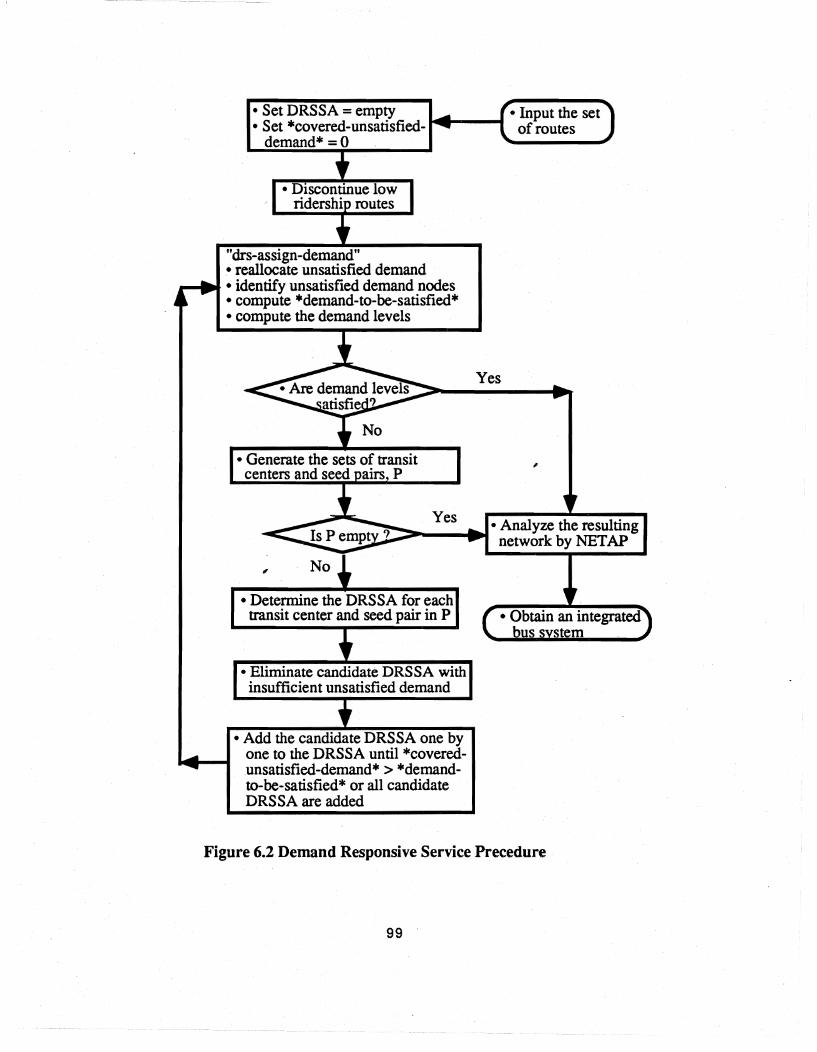
• Set DRSSA = empty • Input the set • Set *covered-unsatisfied- .......... -..... of routes
demand* =0
"drs-as sign-demand " • reallocate unsatisfied demand
r-'" · identify unsatisfied demand nodes • compute *demand-to-be-satisfied* • compute the demand levels
• Generate the sets of transit centers and seed airs P
Yes
,
Yes ~:...._~ ... Analyze the resulting
network by NET AP
• Determine the DRS SA for each transit center and seed pair in P
• Eliminate candidate DRSSA with insufficient unsatisfied demand
• Add the candidate DRS SA one by one to the DRSSA until *coveredunsatisfied-demand * > *demandto-be-satisfied* or all candidate DRSSA are added
• Obtain an integrated bus stem
Figure 6.2 Demand Responsive Service Precedure
99

Step 1 Discontinue low ridership routes, and generate a new set of routes.
Step 2 Call "drs-assign-demand" to reallocate unsatisfied demand, identify unsatisfied
demand nodes, and compute *demand-to-be-satisfied* and the demand levels.
Step 3 If the demand levels are satisfied, go to step 9.
Step 4 Generate sets of transit centers and seed pairs, P.
Step 5 If P is empty, go to Step 9.
Step 6 Determine the candidate DRS service area for each transit center and seed pair in P.
Step 7 Eliminate candidate DRS service areas covering insufficient unsatisfied demand.
Step 8 Add candidate DRS service areas one by one to DRSSA until one of the following
two conditions is met:
a) *covered-unsatisfied-demand* is greater than *demand-to-be-satisfied*.
b) all candidate DRS service areas are selected.
Set *covered-unsatisfied-demand* to zero and go to Step 2.
Step 9 Assign the resulting demand matrix to the fixed route network using the NET AP.
The NIP provides six modifications which include four actions developed by Baa; and
Mahmassani (1991), in addition to route splitting at transit centers, and conversion to demand
responsive service. These actions are implemented in modules which'can be applied individually
or in any sequence. The demand responsive service provides an additional service dimension to
the designer. However, the integration of fixed route and flexible route service increases the
complexity of the bus system. Therefore, the DRS action should be used last in the modification
sequence. ,
Computation of Number of DRS Buses
Once the demand for each DRS route k (DRSOk) has been determined, the procedure then
computes the number of buses required on each DRS route k to achieve the applicable maximum
allowed load factor defined for DRS route:
DRSN = DRSOkDRSTT k k 60.0 * DRS - MAX - LF * *DRS - VEHICLE - SIZE *
where
DRSTTk is the estimated travel time for the DRS route k as described in Section 6.3.3.
*DRS-MAX-LP is the maximum allowed load factor for DRS routes (default is 1.0).
*DRS-VEHICLE-SIZE* is the DRS bus seating capacity (default is 15 seats).
Since DRSNk may not be an integer value, it is rounded up to the closest integer. The minimum
DRS fleet size necessary for the whole DRS system is equal to the sum of DRS buses over all
DRS routes.
100
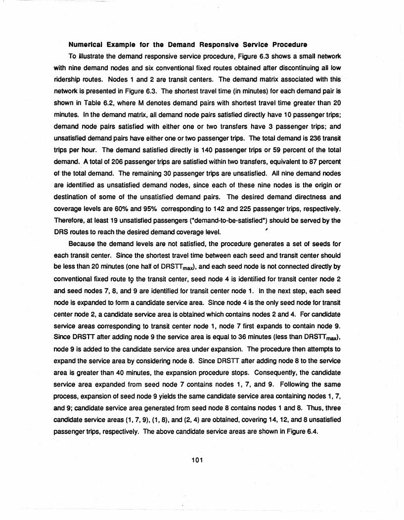
Numerical Example for the Demand Responsive Service Procedure
To illustrate the demand responsive service procedure, Figure 6.3 shows a small network
with nine demand nodes and six conventional fixed routes obtained after discontinuing all low
ridership routes. Nodes 1 and 2 are transit centers. The demand matrix associated with this
network is presented in Figure 6.3. The shortest travel time (in minutes) for each demand pair is
shown in Table 6.2, where M denotes demand pairs with shortest travel time greater than 20
minutes. In the demand matrix, all demand node pairs satisfied directly have 10 passenger trips;
demand node pairs satisfied with either one or two transfers have 3 passenger trips; and
unsatisfied demand pairs have either one or two passenger trips. The total demand is 236 transit
trips per hour. The demand satisfied directly is 140 passenger trips or 59 percent of the total
demand. A total of 206 passenger trips are satisfied within two transfers, equivalent to 87 percent
of the total demand. The remaining 30 passenger trips are unsatisfied. All nine demand nodes
are identified as unsatisfied demand nodes, since each of these nine nodes is the origin or
destination of some of the unsatisfied demand pairs. The deSired demand directness and
coverage levels are 60% and 95% corresponding to 142 and 225 passengertrips, respectively.
Therefore, at least 19 unsatisfied passengers (*demand-to-be-satisfied*) should be served by the
DRS routes to reach the desired demand coverage level. '
Because the demand levels are not satisfied, the procedure generates a set of seeds for
each transit center. Since the shortest travel time between each seed and transit center should
be less than 20 minutes (one half of DRSlT max), and each seed node is not connected directly by
conventional fixed route t9 the transit center, seed node 4 is identified for transit center node 2
and seed nodes 7, 8, and 9 are identified for transit center node 1. In the next step, each seed
node is expanded to form a candidate service area. Since node 4 is the only seed node for transit
center node 2, a candidate service area is obtained which contains nodes 2 and 4. For candidate
service areas corresponding to transit center node 1, node 7 first expands to contain node 9.
Since DRSTT after adding node 9 the service area is equal to 36 minutes (less than DRSTT max),
node 9 is added to the candidate service area under expansion. The procedure then attempts to
expand the service area by considering node 8. Since DRSTT after adding node 8 to the service
area is greater than 40 minutes, the expansion procedure stops. Consequently, the candidate
service area expanded from seed node 7 contains nodes 1, 7, and 9. Following the same
process, expansion of seed node 9 yields the same candidate service area containing nodes 1, 7,
and 9; candidate service area generated from seed node 8 contains nodes 1 and 8. Thus, three
candidate service areas (1, 7, 9), (1,8), and (2, 4) are obtained, covering 14,12, and 8 unsatisfied
passenger trips, respectively. The above candidate service areas are shown in Figure 6.4.
101

Nl N2 N3
Nl 0 10 3
N2 10 0 10
N3 3 ,10 0
N4 3 3 10
N5 10 3 3
N6 10 10 3
N7 3 3 2
N8 2 1 1
N9 2 1 0
R4
Transit Center
Rl
N4 N5
3 10
3 3
10 3
0 2
2 0
3 3
2 10
0 1
0 0
R6
N6
10
10
3
3
3
0
3
1
0
R4
,
N7 N8 N9
3 2 2
3 1 1
2 1 0
2 0 0
10 1 0
3 1 0
0 0 0
0 0 0
0 0 0
Figure 6.3 Network and Transit Demand Matrix for the Illustration of the Demand Responsive Service Procedure
102

Table 6.2 Shonest Travel Time Between Node Pairs For Network
In Figure 6.3
N1 N2 N3 N4 N5 N6 N7 N8 N9
N1 0 M M M 10 10 15 10 15
N2 M 0 10 15 M M M M M
N3 M 10 0 5 M M M M M
N4 M 15 5 0 M M M M M
N5 10 M M M 0 20 5 5 M
N6 10 M M M 20 0 M 20 10
N7 15 M M M 5 M 0 M 5
N8 15 M M M M 10 M 0 M
N9 10 M M M 5 20 5 M 0
Shortest Travel Times are in minutes , M denotes shortest travel time greater than 20 minutes
Table 6.3 New Demand Matrix for Fixed Route Service After the
Reallocation of Unsatisfied Demand , N1 N2 N3 N4 N5 N6 N7 N8 N9
N1 M M M 10 10 15 10 15
N2 0 10 15 M M M M M
N3 10 0 5 M M M M M
N4 15 5 0 M M M M M
N5 M M M 0 20 5 5 M
N6 M M M 20 0 M 20 10
N7 M M M 5 M 0 M 5
N8 M M M M 10 M 0 M
N9 M M M 5 20 5 M 0
103
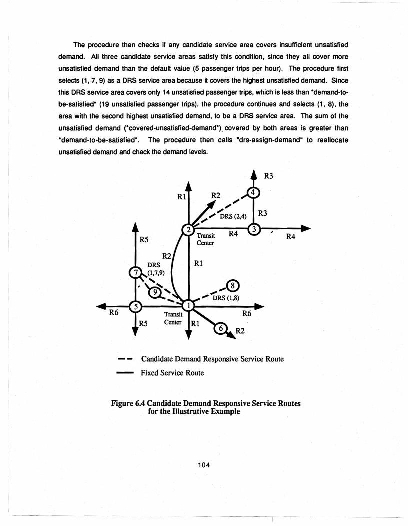
The procedure then checks if any candidate service area covers insufficient unsatisfied
demand. All three candidate service areas satisfy this condition, since they all cover more
unsatisfied demand than the default value (5 passenger trips per hour). The procedure first
selects (1,7,9) as a DRS service area because it covers the highest unsatisfied demand. Since
this DRS service area covers only 14 unsatisfied passenger trips, which is less than *dernand-to
be-satisfied* (19 unsatisfied passenger trips), the procedure continues and selects (1, 8), the
area with the second highest unsatisfied demand, to be a DRS service area. The sum of the
unsatisfied demand (*covered-unsatisfied-demand*). covered by both areas is greater than
*demand-to-be-satisfied*. The procedure then calls "drs-assign-demand" to reallocate
unsatisfied demand and check the demand levels.
R3
; ;;
;; DRS(2,4)
R4 , R4
Rl
-,0 -' _ .. __ -' DRS (1,8)
R6
- - Candidate Demand Responsive Service Route
- Fixed Service Route
Figure 6.4 Candidate Demand Responsive Service Routes for the Illustrative Example
104
I·
The new integrated system contains six conventional fixed routes and two DRS routes. To
illustrate -drs-assign-demand-, four unsatisfied demand pairs (1, 8), (2; 9),(3, 7), (4,7) are used as
examples. The demand of (1, 8) is satisfied directly by DRS route (1, 8). Therefore, *DEMAND-O
TRANSFER· is updated by adding 2 passenger trips; no adjustment to the demand matrix is
needed. Demand pair (2, 9) is satisfied with one transfer. Passengers between this demand pair
board either R1 or R2 at node 2, and stay on until node 1, where they transfer to DRS route (1, 7,
9), and travel on it until node 9. *DEMAND-t-TRANSFER* is updated by adding 1 passenger trip.
Since the passengers between demand node pair (2, 9) use fixed routes from node 2 to node 1,
the demand of (2, 1) is increased by 1 passenger trip, and the demand of (2, 9) is set to zero in the
demand matrix. Demand pair (3, 7) is satisfied with two transfers. Passengers between this
demand node pair board R4 at node 3, stay on it until node 2, then transfer to either R1 or R2,
travel on them until node 1, where the passengers transfer to DRS route (1, 7,9), and stay on it
until node 7. ·DEMAND-2-TRANSFER* is updated by adding 2 passenger trips. The demand
between (3, 1) is increased by 2 passenger trips, and the demand between (3, 7) is set to zero in
the demand matrix. Demand pair (4, 7) remains unsatisfied in the new integrated system,· since
more then two transfers are needed. After executing "drs-assign-demand-, a new demand matrix
for the conventional fixed route service is obtained as shown in Table ff.3. Four demand pairs (4,
5). (4, 7), (5,4), and (7,4) remain unsatisfied. Demand pairs (1, 8), (1, 9), (8, 1), and (9, 1) are not
satisfied by the conventional fixed routes, but satisfied directly by the DRS routes. The demand
directness and coverage levels for the integrated bus system are 63% and 97%, respectively.
Since both demand levels are greater than the desired levels, no additional DRS route needs to , be generated.
In the trip assignment process, the demand for DRS routes (1, 7, 9) and (1, 8) are found to be
10 and 12 passenger trips per hour, respectively. Travel times for the above two routes are
estimated to be 30 and 36 minutes. From the equation for computing the number of buses
required on each DRS route described in Section 6.3.4, 0.4 buses are required for each DRS
route. By rounding up to the closest integer value, both DRS routes require one bus.
SUMMARY
This chapter describes the transit center selection and network improvement procedures.
The transit center selection procedure identifies suitable transit centers that are utilized in the
design of timed-transfer service and demand responsive service. The network improvement
procedures modify networks generated by the RGP and NETAP so that better system
effectiveness and service levels can be achieved.
105

CHAPTER 7. COMPUTATIONAL EXPERIMENTS
INTRODUCTION
The transit network design framework incorporates four main procedures, namely, the route
generation procedure (RGP), network analysis procedure (NETAP). transit center selection
procedure (TCSP), and network improvement procedures (NIP), all of which have been described
in the previous chapters. Using these procedures, alternative design concepts, including
conventional systems, coordinated services. integrated systems, and variable vehicle sizes are
implemented in the solution framework as described in Chapter 3. In this chapter, the results of
extensive computational experiments are presented to test and illustrate the above design
procedures and alternative design features on cases representing different levels and spatial
distributions of demand.
The computational tests have two primary objectives. The first is to investigate and compare
the character and performance of the solution networks generated with the transit center concept
relative to other proposed solutions, namely those generated by Mandl's and Baa; and
Mahmassani's algorithms. for·a benchmark problem. The second objective is to test the solution
framework and investigate its performance with respect to an actual transit network. This objective , is achieved by testing the design procedures and alternative design concepts with data
generated for the transit system of Austin, Texas. In addition, sensitivity analyses with respect to
key design features and parameters of the procedures are performed. The design features
tested include uncoordinated "s. coordinated, fixed vs. variable vehicle sizes, and conventional
fixed route vs. integrated services; the design parameters tested include minimum system
directness level, minimum system coverage level, application strategy for the TCSP, and
acceptable splitting ratio.
The benchmark network was originally reported by Mandl (1976) and tested by Baaj and
Mahmassani (1991) for comparison. The network is small and dense; it comprises only 15 nodes
within a 33 minute shortest travel distance between the two furthest nodes. Although this
network may not be very representative of many real-world urban bus transit networks, it is still
useful possibly as a regional subnetwork. The demand matrix used by Mandl and Baaj and
Mahmassani contains relatively heavy ridership. This base network was used to test the solution
framework during the development stage. In the next section, the solutions to the benchmark
transit network are reported and compared to the solutions of Mandl's and Baaj and Mahmassani's
algorithms.
In section 7.3, the design procedures and alternative design concepts are tested with data
from the Austin transit system. Six different combinations of the desired minimum system
106

coverage and directness levels are used for the tests. Section 7.3.1 presents tests of the transit
center selection procedure (TCSP). Sets of transit centers generated from the different
combinations and from dHferent application strategies are reported and investigated. In Section
7.3.2, the route generation procedure (RGP) and network analysis procedure (NETAP) are tested
in a performance comparison of four design alternatives: uncoordinated design with fixed vehicle
size, uncoordinated design with variable bus sizes, coordinated design with fixed vehicle size,
and coordinated design with variable vehicle sizes. The comparison is based on four categories
of performance measures: 1) demand satisfaction levels, 2) user travel costs, 3) operator costs,
and 4) total system cost. In Section 7.3.3, the modification procedure which splits routes at transit
centers for the coordinated network is tested and its sensitivity to the value of the acceptable
splitting ratio is analyzed. Section 7.3.4 describes the performance of the "integrated" system
design that allows for demand responsive service as a modification to two of the solutions
presented in Section 7.3.2. Section 7.3.5 presents a summary discussing the conclusions of the
computational experiments with the data from the transit system of Austin, Texas.
EXPERIMENTS ON BENCHMARK PROBLEM Mandl's transit network is based on a real network in Switzerland., There are no acceptable
benchmark networks in the transit network design literature, and Mandl.'s is the only one for which
the author has reported all pertinent information to allow replication and comparative testing,
making it a de facto benchmark. This network has been utilized by Baaj and Mahmassani as a
benchmark problem to compare their results with Mandl's solutions. In this section, the
performance of the solution networks generated by the route generation procedure (RGP) with
the transit center concept are investigated using this same network.
Mandl's Transit Network
In Figure 7.1, the network connectivity and demand matrix for Mandl's SwiSS network are
shown. The in-vehicle travel time between two adjacent nodes is in minutes. The demand matrix
shows the average number of passenger trips per day for each transit node pair. The total
demand is 15570 transit trips; the highest node pair demand is 880 transit trips. In this matrix,
82% of the demand node pairs have non-zero demands.
Mandl presented two solutions (before and after improveme.nt) which satisfied 100% of the
total demand in the given network. Figure 7.2 shows Mandl's final solution network after
improvement. Baaj and Mahmassani produced three solutions for this network shown in Figure
7.3, Figure 7.4, and Figure 7.5, and compared them to Mandl's solutions. Their solutions
107

8 (in-vehicle travel time, minutes) 2
Transit Demand Matrix in List Form;
(0400 200 60 80 15075 75 30 1603025 35 00) (400 0 561202018090 9015 13020101050) (200 50 0 40 60 1809090 1545 20 10 105 0) (60 120 40 0 50 100 5050 15 24040 25 10 5 0) (802060500502525 10120 2015500) (150180180100 50 0100 100 30 880 6015 15 100) (75 90905025 100 0 50 15 44035 10 105 0) (75 90905025 100 500 15 44035 10 105 0) (30 15 15 15 1030 15 15 0 140 205 000) (160 13045 240 120 880440440 1400600 250 500 200 0) (30 20 20 4020 60 35 35 20 600 075 95 15 0) (25 101025 15 15 101052507507000) (35 1010105 15 10100500 95700450) (05550105502001504500) (0 0 0 0 0 0 0 0 0 0 0 0 0 0 0)
Figure 7.1 Mandl's Swiss Network and Transit Demand Matrix
108

[!jJ:1inks served by route rl Route rl: 0-1-2-5-7-9-10-12 Route r2: 4-3-5-7-14-6 Route r3: 11-3-5-14-8 Route r4: 12-13-9
Figure 7.2 Route Layout Generated by Mandl's Algorithm
109
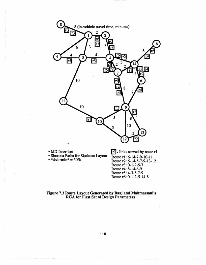
• MD Insertion • Shortest Paths for Skeleton Layout • *dsdinnin* = 50%
I!D: links served by route rl Route r1: 6-14-7-9-10-11 Route r2: 6-14-5-7-9-13-12 Route r3: 0-1-2-5-7 Route r4: 8-14-6-9 Route r5: 4-3-5-7-9 Route r6: 0-1-2-5-14-8
Figure 7.3 Route Layout Generated by Baaj and Mahmassani's RGA for First Set of Design Parameters
110

_~~ 8 (in-vehicle travel time, minutes)
,
• MDMT Insertion • Alternate Shortest Paths
for Skeleton Layout • *dsdinnin* = 50%
r8
2
,
(!11: links served by route r 1 Route r1: 0-1-3-11-10-12-13 Route r2: 2-5-7-14-6-9 Route r3: 9-10-12 Route r4: 9-10-11 Route r5: 7-9-13 Route r6: 0-1-3-5 Route r7: 8-14-5-7-9 Route r8: 4-1-2-5-14-6-9
Figure 7.4 Route Layout Generated by Baaj and Mahmassani's RGA for Second Set of Design Parameters
111

• MD Insertion • Shortest Paths for Skeleton Layout • *dsdinnin* = 70%
[!!J: links served by route rl Route rl: 9-12 Route r2: 9-10-11 Route r3: 9-3 Route r4: 0-1-2-5-7-9 Route r5: 8-14-6-9 Route r6: 4-3-5-7-9 Route r7: 0-1-3-4
Figure 7.s Route Layout Generated by Baaj and Mahmassani's RGA for Third Set of Design Parameters
112

dominated the networks generated by Mandl's design algorithm in terms of the levels of demand
satisfaction, in-vehicle travel time, and required resource (fleet size) but not in terms of the total
waiting time. In the following section, the solutions generated by the RGP with the transit center
concept for coordinated and uncoordinated service are compared to Mandl's and Baaj and
Mahmassani's solutions for uncoordinated transit network designs.
The solutions were generated by RGP using the same three sets of design parameters that
were tested by Baaj and Mahmassani. These are summarized in Table 7.1. In the first case, the
desired minimum system directness level (the minimum total demand satisfied directly, *dsdirmin*)
was set at 50%, the shortest path was used for the initial layout of skeletons, and the maximum
demand (MO) node selection and insertion heuristic was followed. In the second case, the same
*dsdirmin* was specified, the alternate shortest path was used to form skeletons where feasible,
and the maximum demand per minimum time (MDMT) insertion heuristic was employed. The third
case increased the desired minimum system directness level (*dsdirmin*) to 70% and used the
shortest path and the MD heuristic. The desired minimum system coverage level (the minimum
total demand satisfied, *dsmin*) for all three cases was set to 100%.
, Table 7.1 Summary of Design Parameters for Three Test Cases
Minimum Minimum . System Skeleton Insertion System
Case directness Formation Heuristic Coverage
level level
shortest path -
1 50% MD 100%
2 50% alternate
MDMT 100%. shortest path
3 70% shortest path MD 100%
The resulting sets of routes from the RGP were evaluated using the NETAP for both
coordinated and uncoordinated designs. The NETAP was also used to evaluate all the solutions
suggested by Mandl as well as by Baaj and Mahmassani. In all the NETAP runs, the bus seating
capacity was selected at 40 seats, the transfer penalty was set at 5 minutes of in-vehicle travel
time, and a bus load factor of 1.25 was selected. Operation cost coefficients, a and b, were set to
2.962 and 0.0078, respectively, the same values used in the illustrative application for Austin
113

case in Section 5.7. The minimum separation distance (travel time) between transit centers was
selected to be 10 minutes; the minimum total demand for a transit center was set to 100
passengers; the minimum demand covered by a transit center was set to 150 passengers.
Numerical Results and Conclusions
Two sets of routes were generated by the RGP using the above three sets of input design
parameters, as the route networks generated for the first and third cases are the same. Figures
7.6 and 7.7 show the networks generated by the RGP. Tables 7.2, 7.3, and 7.4 show the results
of the solutions generated by the RGP and by Baaj and Mahmassani's algorithms using the first,
second, and third sets of design parameters, respectively, as well as Mandl's final solution.
All the networks generated by the RGP for the different sets of design parameters had a
higher percentage of total demand satisfied directly (82.59, 87.73, and 82.59) than Baaj and
Mahmassani's solutions (78.61, 79.96, and 80.99) and Mandl's solution (69.94). Consequently,
the percentage of transferring passengers was less in aU three of the RGP solutions (17.4, 12.27,
and 17.4) than Baaj and Mahmassani's (21.39,20.04, and 19.04) and Mandl's (30.06).
In all networks utilizing the timed-transfer (route coordination) concept, the total in-vehicle
travel limes were much higher than Baaj and Mahmassani's and Mandl"s solutions. In the worst
case, the total in-vehicle travel time was 14% more than Baaj and Mahmassani's solution and 8%
more than Mandl's solution. As a result, higher total travel times were required by the timed
transfer cases. The increase of in-vehicle time resulted from additional in-vehicle waiting incurred
by passengers who remaip on board at transit centers during a time window (for coordinated
operations). The additional in-vehicle waiting times for the three timed-transfer networks were
20933, 19574, and 20933 minutes, respectively, based on a five-minute time window. One may
reduce this in-vehicle time by using a smaller time window, which however will increase the
possibility of missing connections. Therefore, the reliability of bus operations must be traded-off
against in-vehicle as well as out-of-vehicle waiting time in determining the time window for
coordination at the transit centers. The cases with coordinated route operation had lower out-of
vehicle waiting time than Baaj and Mahmassani's solutions. The differences ranged from 6% to
16%. Mandl's solution had a total out-of-vehicle waiting time that was 8% lower than the best case
of timed-transfer networks because the service frequencies on Mandl's routes were much higher
than all the coordinated networks. All the coordinated networks had lower aggregate transfer
penalties (time) than Baaj and Mahmassani's solutions (39 % lower in the best case) and Mandl's
solution (59% lower). The computation of the aggregate transfer penalty was based on the
assumption that each transfer is equivalent to five minutes of in-vehicle travel time. It might be
114
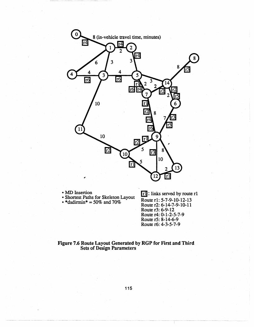
• MD Insertion • Shortest Paths for Skeleton Layout • *dsdinnin* = 50% and 70%
(!]: links served by route rl Route rl: 5-7-9-10-12-13 Route r2: 6-14-7-9-10-11 Route r3: 6-9-12 Route r4: 0-1-2-5-7-9 Route r5: 8-14-6-9 Route r6: 4-3-5-7-9
Figure 7.6 Route Layout Generated by RGP for First and Third Sets of Design Parameters
115
- - - - -------- - - --- ------ - - --------

• MDMT Insertion • Alternate Shortest Paths for Skeleton Layout
• *dsdirmin* = 50%
1!lI: links served by route rl Route rl: 2-5-14-6-9-10 Route r2: 1-2-5-7-14-6-9-10 Route r3: 9-13-12 Route r4: 0-1-3-5 Route r5: 9-10-11 Route r6: 8-14-6-9 Route r7: 4-3-5-7-9 Route r8: 0-1-2-5-7-9-12
Figure 7.7 Route Layout Generated by RGP for Second Set of Design Parameters
116

!
..... ..... -..J.
Table 7.2 Comparison of Solutions for the Benchmark Network for Cases Using Fisrt Set of Design Parameters
RGP with Transit Center Concept Baajand Network Characteristics Mahmassani's
Coordinated Uncoordinated Solution ..
% demand O-transfer 82.59 82.59 78.61
% demand 1-transfer 17.41 17.41 21.39
% demand 2-transfer 0 0 0
% total demand unsatisfied 0 0 0
Total travel time (minutes) 225102 203936 205646
Total in-vehicle-travel time 191826 170328 168077
In-vehicle waiting time 20933 -- --Total out-d-vehicle wa~ing time 19726 20058 20920
Total transfer time (penalty) 13550 13550 16650
Fleet size 87 84 89
Operation cost ($) 4043.14 3924,26 4163.46
Fuel consumption (gallons) 346.8 336.6 357.12
First set of input design parameters: 50 % minimum total demand satisfied directly, MD node insertion strategy, and Shortest path heuristic
Mandl's Solution
I
69.94 I
29.93
0.13
0
219094
177400
--18194
23500
99
4620.61
396.33
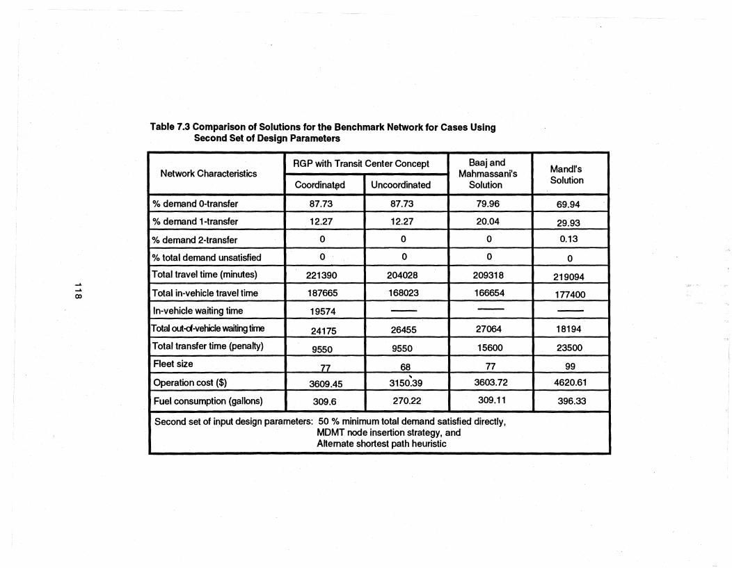
-" -' (Xl
Table 7.3 Comparison of Solutions for the Benchmark Network for Cases Using Second Set of Design Parameters
RGP with Transit Center Concept Baajand Network Characteristics Mahmassani's
Coordinat~d Uncoordinated Solution
% demand O-transfer 87.73 87.73 79.96
% demand 1-transfer 12~27 12.27 20.04
% demand 2-transfer 0 0 0
% total demand unsatisfied 0 0 0
Total travel time (minutes) 221390 204028 209318
Total in-vehicle travel time 187665 168023 166654
In-vehicle waiting time 19574 -- -Total out-d-vehicle waiting time 24175 26455 27064
Total transfer time (penalty) 9550 9550 15600
Fleet size 77 68 77
Operation cost ($) 3609.45 ..
3150.39 3603.72
Fuel consumption (gallons) 309.6 270.22 309.11
Second set of input design parameters: 50 % minimum total demand satisfied directly, MDMT node insertion strategy, and Alternate shortest path heuristic
Mandl's Solution
69.94
29.93
0.13
0 .
219094
177400
--18194
23500
99
4620.61
396.33

---J
..... ..... co
Table 7.4 Comparison of Solutions for the Benchmark Network for Cases Using Third Set of Design Parameters
RGP with Transit Center Concept 8aajand Network Characteristics Mahmassani's
Coordinctted Uncoordinated Solution
% demand O-transfer 82.59 82.59 80.99
% demand 1-transfer 17.41 17.41 19.01
% demand 2-transfer 0 0 0
% total demand unsatisfied 0 0 0
Total travel time (minutes) 225102 203936 217954
Total in-vehicle travel time 191826 170328 180350
In-vehicle waiting time 20933 -- --Total out-of-vehicle wa~ing time 19726 20058 22804
Total transfer time (penalty) 13550 13550 14800
Fleet size 87 84 82
Operation cost ($) 4043.14 3924.26 3830.03
Fuel consumption (gallons) 346.8 336.6 328.52
Third set of input design parameters: 70 % minimum total demand satisfied directly, MD node insertion strategy, and Shortest path heuristic
Mandl's Solution
69.94
29.93
0.13
0
219094
177400
--18194
23500
99
4620.61
396.33

more appropriate to use a lower transfer penalty for transfers completed under route coordination;
the total transfer penalty for the coordinated networks would have then been lower than the
results presented.
All the timed-transfer networks required smaller fleet sizes (87, n, and 87 buses) than
Mandl's network (99 buses). In comparison with Baaj and Mahmassani's solutions, the
coordinated design required a smaller fleet Size (87 vs. 89 buses) for the first case, the same fleet
Size (87 buses) for the second case, and a larger fleet size (87 vs. 82 buses) for the third case.
The same patterns were observed for the operation cost and total fuel consumption. For the first
case, the timed-transfer design required lower operation cost ($4043 vs. $4163) and fuel
consumption (347 vs. 357 gallons) than Baaj and Mahmassani's design. For the second case, the
operation cost and fuel consumption for the two designs are nearly the same. For the last case,
the timed-transfer network required higher operation cost ($4043 vs. $3830) and fuel
consumption (347 vs. 329 gallons) than Baaj and Mahmassani's design. Mandl's solution resulted
in both the highest operation cost ($4620) and fuel consumption (396 gallons).
All the uncoordinated networks generated by the RGP using the transit center concept
outperformed the· solution network proposed by Mandl in all aspects except the total waiting time
component. The required fleet size varied from 68% to 85% of that proposed by Mandl. The
operation cost and fuel consumption savings ranged from 15% to 32%. The total travel times
were lower by about 7% in all three cases; the in-vehicle travel times were 4% to 6% lower. The
total out-of-vehicle waiting time for Mandl's network was lower by about 9% to 31% than those of
the resulting networks beca)Jse of the higher frequencies.
The RGP designs also outperformed Baaj and Mahmassani's solutions with the exception of
the in-vehicle travel time for the first and second cases and the operator costs for the third case.
The required fleet sizes for the RGPsolutions were smaller in the first and second cases than Baaj
and Mahmassani's solutions (84 vs. 89 and 68 vs. n), but Slightly higher in the third case (84 vs.
82). Similarly, the operation costs were lower in the first two cases ($3924 vs. $4163 and $3150
vs. $3604) and worse in the third case ($3924 vs. $3830). Following the same pattern, the fuel
consumption was lower for the first two cases (337 vs. 357 and 270 vs. 309 gallons)· and higher in
the last case (337 vs. 329 gallons). The total travel time was at worst slightly lower than that of Baaj
and Mahmassani (0.8%) and in the best case 6% lower. The total out-of-vehicle waiting times for
all cases were better by about 2% to 12% than those of Baaj and Mahmassani's solutions. The in
vehicle travel times in the first two cases were slightly higher (approximately 1 %) than in Baaj and
Mahmassani's solutions, but 6% lower in the third case.
120

In summary, the networks generated around the transit center concept had better
performance in terms of the levels of demand satisfaction for all study cases. The timed-transfer
design reduced the total passenger out~of-vehicle waiting time in all cases compared to Baaj and
Mahmassani's solution (19726 vs. 20920, 24175 vs. 27064, and 19726 vs. 22804 minutes), but
required very high additional in-vehicle waiting time in all three cases (23749, 21011, and 11476
minutes, respectively) due to the route coordination. The uncoordinated networks generated
with the transit center concept had solutions that outperformed the solutions proposed by Mancil
and by Baaj and Mahmassani. Overall, in comparison with Mandl's solution, the best
uncoordinated network satisfied 18% more passengers directly with approximately 32% fewer
buses, lower operation cost, and less fuel consumption, and 7% less total travel time. In
comparison with Baaj and Mahmassani's solutions, the best case satisfied 8% more passengers
directly with 12% fewer buses, lower operation cost, and less fuel consumption and, 2.5% less
total travel time.
The benchmark network used in this section was small and dense with only 15 nodes within a
33 minute shortest travel distance between the two furthest nodes and with a total demand of
15570 trips per day. With this relatively high demand density, aU the passengers in this network
were served with a high level of service and had high frequencies of service on all routes. It has
been shown in this section that conventional uncoordinated, fixed-route and fixed-schedule bus
service is suitable for this type of network. Coordination has less impact on networks with high
frequency routes because it tends to increase in high in-vehicle time with limited opportunity for
out-of-vehicle waiting tim9 saving. Demand-responsive service is not particularly suitable for this
type of system. As discussed by Baaj (1990), constraints on route length, route circuity, and
route duplication may not affect the search in a small network such as Mandl's, but will tend to be
more important in medium to large networks. As a result, concluSions obtained on the basis of this
network may not necessarily be applicable to actual networks. Therefore, the design procedures
and alternative design concepts in the solution framework should be tested in actual networks. In
the next section, the tests of the proposed design procedures and alternative design concepts
are performed with the data generated for the transit network of Austin, Texas.
TESTS ON THE AUSTIN TRANSIT NETWORK
In this section, the design procedures and alternative design concepts of the solution
framework are tested with the data generated from the transit system of Austin, Texas. The
network data for this application was discussed in Section 4.7.1, and includes the transit demand
matrix, the network connectivity, and the lists of the shortest paths and k shortest paths for all the
121

transit node pairs. Several user specified parameters for the execution of the numerical
experiments on the Austin case are listed in Table 7.S. The experiments are performed with six
combinations of minimum system coverage (·dsmin·) and directness (·dsdirmin·) levels to
investigate the performance of the design procedures and alternative design concepts. Table
7.6 lists the six combinations of the two user desired minimum demand levels.
The computational experiments address the following four objectives:
1) Investigate the TCSP, described in Chapter 6. The sets of transit centers obtained for
different combinations of desired minimum system coverage and directness levels and from
different application strategies (one-pass vs. iterative process) are presented and compared in
Section 7.3.1.
2) Test the RGP and NETAP and investigate the performance of fixed route designs for
different combinations of minimum system coverage and directness levels. Route networks
generated to satisfy a lower minimum system coverage level generally serve areas with high
demand and leave spatially dispersed demand unsatisfied, whereas networks generated to
provide greater demand coverage naturally serve more spatially dispersed demand. Therefore,
alternative design concepts can be tested for different spatial distributions of demand by altering
the minimum system coverage level. In addition, route networks generated by the RGP perform
differently for alternative designs with different system directness levels. The effect of the system
directness level are also examined. In Section 7.3.2, the performance of four alternative fixed
route deSigns are investigated under different combinations of minimum demand levels. The
alternative designs are: uncoordinated design with fixed vehicle size, uncoordinated design with "
variable vehicle sizes, coordinated design with fixed vehicle size, and coordinated design with
variable vehicle sizes.
3) Investigate the effects of the proposed route splitting procedure on coordinated systems.
This procedure is intended to improve the system effectiveness by splitting routes at transit
centers and reducing the negative effect (transfer waiting time) of route coordination. Section
7.3.3 shows the results of the procedure and discusses their sensitivity to the value of the
splitting indicator.
4) Investigate performance of the integrated bus system proposed in the solution framework.
The integrated bus system serves high demand density areas with fixed route service and low
demand density areas with demand responsive service. The intent is to examine the performance
of the demand responsive service procedure. Results of the integrated bus system design tests
are presented in Section 7.3.4.
122

Table 7.5 User Specified Parameters for Experiments on the Austin Network
Set of terminal nodes
Skeleton layout heuristic
Node insertion strategy
Number of initial skeletons
25 for *dsmin* = 60
40 for *dsmin* = 80
Maximum operational frequency
Minimum allowable bus frequency
Maximum load factor
none
shortest path
maximum demand per minimum route length increase
(MDML) heuristic
15 for *dsmin* = 40
20 buses/hour
1 bus/hour
1.25 on routes with frequency more than 2 buses/hour
0.80 on routes with frequency less than 2 buses/hour
Transfer penalty 5 minutes of equivalent in-vehicle travel time
Bus seating capacity 40 passengers for fixed bus size option
Available commercial vehicle sizes
Fuel consumption coefficients
Operation cost coefficient, a
Operation cost coefficient, b
Minimum separation travel time
between two transit centers
Minimum demand covered by
a transit center
Waiting time value
In-vehicle travel time value
Tests of the TCSP
15, 27, and 37 seats for variable bus size option
3,6, and 9 miles per gallon for vehicles with 37,27, and
15 seats, respective.
2.962
0.0078
15 minutes
150 passengers/hour
$9/hour
$3/hour
,
As described in Section 6.2, the TCSP may be applied in two different ways to identify sets
of transit centers for a given system. The first application strategy conSists of executing the
procedure in a single pass (i.e. one iteration only). The second consists of executing the
procedure iteratively until the set of transit centers converges. In Table 7.7, the results obtained
for different combinations of application strategies and minimum system coverage and directness
levels are reported. A total of twelve different sets of transit centers were generated by the TCSP
for evaluation.
123

Table 7.6 Six Selected Combinations of Minimum System Coverage and
Directness Levels
Minimum System Directness Level
*dsdinnin* (%)
40
40
60
60
80
80
Minimum System Coverage Level
*dsmin* (%)
80
98
80
98
80
98
The TCSP produced consistent solutions in the numerical experiments. The results show
that six transit nodes, (2,9,19,36, 78, 84), were identified as transit centers in all the study cases.
Transit nodes 87 and 101 were identified as transit centers in eleven out of the twelve cases.
Except for the combination of 40% minimum system directness and 80% minimum system
coverage, the sets of transit centers identified by the TCSP were nearly the same with only two
transit nodes, 42 and 87, alternating with each other in those cases. The number of iterations to
reach convergence for each combination of desired demand levels is also shown in Table7.7. In
the worst case (40% minimum system directness and 80% of minimum system coverage), four
runs were needed. For three out of six demand cor:nbinations, convergence to the same set of
transit centers was obtained in only two iterations. For two demand combinations, only one transit , center was different between the two sets generated by a single pass versus the convergent
iterative process. Even in the worst case, only two transit centers were different.
Transit centers identified by the TCSP contained a downtown transit center, major shopping
malls or centers in the city, and transit nodes serving major population clusters or communities in
the suburban areas. Among the selected centers, node 2 is the major transit station in the
downtown area; nodes 19 and 36 correspond to major activity centers, Northcross Mall and
Highland Mall in the north; node 84 is at Westgate Mall, a major shopping center in the south.
Node 9 is located at a commercial center surrounded by major residential areas in the far north of
the city. Since nodes 42 and 87 are close to each other in the east of the city, each set of transit
centers contains only one of these two nodes so as to meet the separation criterion. The total
node demand criterion determines which of these two nodes should be selected. Nodes 57,73,
and 121 cover major residential areas and are located at major arterial intersections and shopping
centers in the far south of the city.
124

--I\) (]'I
Table 7.7 Sets of Transit Centers Generated by TCSP for Different Combinations of Minimum System Coverage and Directness Levels & Terminating Strategies
Desired demand Set of transit centers Set of transit centers Iterations to reach levels for one iteration after convergence convergence
*dsdirmin* = 40% 2,9,19,36,57, 78, 8~, 2,9,19,36,57,78,84,87 *dsmin* = 80% 87, 101, 121
4
*dsdirmin* = 40% 2, 9, 19, 36,42, 73, 2, 9, 19, 36, 73, 78, 3 *dsmin* = 98% 78,84,101 84,87,101
*dsdirmin* = 60% 2,9, 19,36,73, 78, 2,9,19,36,73,78, 2
*dsmin* = 80% 84,87,101 84,87,101
*dsdirmin* = 60% 2,9,19,36,42,73, 2,9,19,36,73,78, 3 *dsmin* = 98% 78,84,101 84,87,101
*dsdirmin* = 80% 2,9,19,36,73,78, 2,9,19,36,73,78, 2
*dsmin* = 80% 84,87,101 84,87,101
*dsdirmin* = 80% " 2, 9, 19, 36,42, 73, 2,9,19,36,42,73, *dsmin* = 98% 78,84,101 78,84,101 2
- - ----
Tests of the RGP and NETAP
In this section, the RGP and the NETAP were tested on the transit network data of Austin,
Texas. Experiments were performed on the four types fixed-route, fixed-schedule service
designs described in the solution framework: uncoordinated network with fixed vehicle size,
uncoordinated network with variable vehicle sizes, coordinated network with fixed vehicle size,
and coordinated network with variable vehicle sizes. These four design types were investigated
under six selected combinations of minimum system coverage and directness levels to
accomplish the second objective described in Section 7.3. The six combinations are the same
ones used in the TeSp tests.
For each uncoordinated design, oneRGP run and one NETAP run were required. The
TeSp was first utilized to generate a set of transit centers for the coordinated design. In all the
experiments, the set of transit centers was generated with a single pass of the TeSp, each of
which required one RGP run and one NETAP run. Therefore, each coordinated design required
two RGP, and two NETAP runs. Since six combinations of minimum system coverage and
directness levels were tested, the two uncoordinated designs required 12 runs and the two
coordinated designs required 24 runs,for a total of 36 RGP runs and 36 NETAP runs.
The numerical results were compared according to four categories of performance
measures: 1) demand satisfaction levels, 2) user travel costs, 3) operation costs, and 4) total
system cost. Demand satisfaction levels used for the comparison are the percentages of demand
satisfied directly, demand satisfied with one transfer, and total demand satisfied. User travel costs
considered include total in;,vehicle travel time, average passenger in-vehicle travel time, total out
of-vehicle waiting time, average passenger out-of-vehicle waiting time, total transfer penalty, and
total travel time. Total fuel consumption and total operation cost are the operation costs
performance measures used for the comparison. The total system cost components are the total
user cost and total operation cost. In each of the following figures, the output variable of interest
is plotted for the different levels of the user specified design parameters, namely the minimum
system coverage at levels of 80 and 98% and minimum system directness at levels of 40, 50, and
80%. Values are shown for both coordinated networks and uncoordinated networks and in some
cases for fixed and variable vehicle sizes.
126

-'it ->-;: u CD .: c '0 !! -'" ;: as (I)
'0 C as E CD C -0
CD CD as -c CD ~ CD a..
U uncoordinated networks
C coordinated networks
80% minimum system coverage 98% minimum system coverage
90~------------------------------------~
80
70
, 60
50~------~~-------r--------r-------~ 20 40 60 80 100
Minimum System Directness Level (%)
Figure 7.8 Percentage of Demand Satisfied Directly vs. Minimum System Directness Level
127
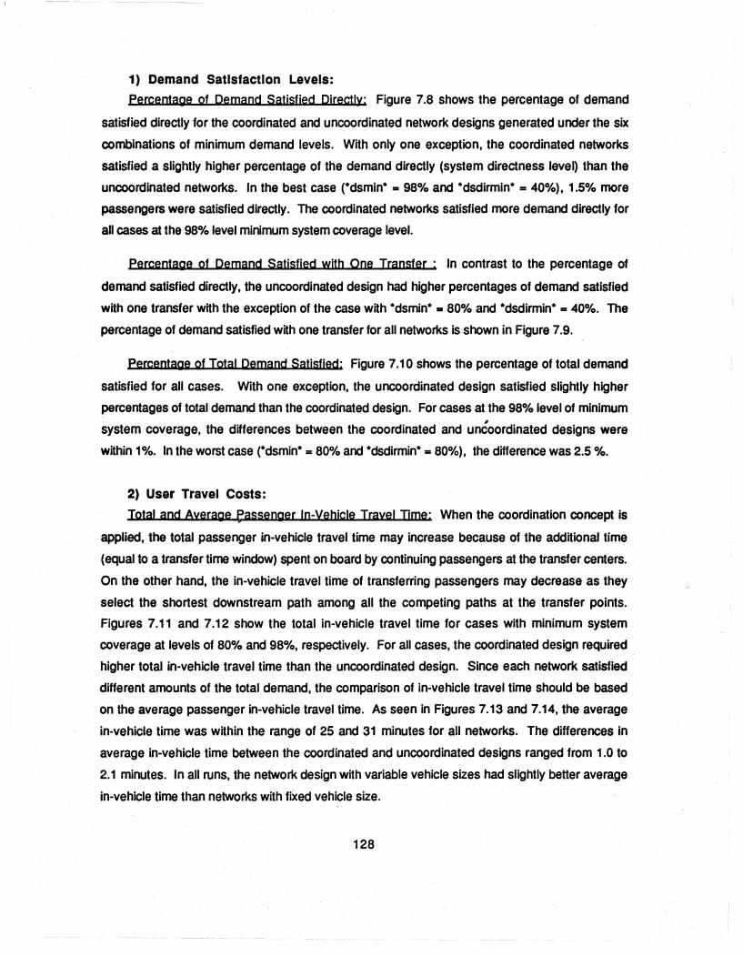
1) Demand Satisfaction Levels:
Percentage of Demand Satisfied Directly: Figure 7.8 shows the percentage of demand
satisfied directly for the coordinated and uncoordinated network designs generated under the six
combinations of minimum demand levels. With only one exception, the coordinated networks
satisfied a slightly higher percentage of the demand directly (system directness level) than the
uncoordinated networks. In the best case (*dsmin* = 98% and *dsdirmin* = 40%), 1.5% more
passengers were satisfied directly. The coordinated networks satisfied more demand directly for
all cases at the 98% level minimum system coverage level.
Percentage of Demand Satisfied with One Transfer' In contrast to the percentage of
demand satisfied directly, the uncoordinated design had higher percentages of demand satisfied
with one transfer with the exception of the case with *dsmin* - 80% and *dsdirmin* = 40%. The
percentage of demand satisfied with one transfer for all networks is shown in Figure 7.9.
Percentage of Total Demand Satisfied: Figure 7.10 shows the percentage of total demand
satisfied for all cases. With one exception, the uncoordinated design satisfied slightly higher
percentages of total demand than the coordinated design. For cases at the 98% level of minimum ,
system coverage, the differences between the coordinated and uncoordinated designs were
within 1%. In the worst case (*dsmin* = 80% and *dsdirmin* = 80%), the difference was 2.5 %.
2) User Travel Costs:
Total and Ayerage eassenger In-Vehicle Trayel Time: When the coordination concept is
applied, the total passenger in-vehicle travel time may increase because of the additional time
(equal to a transfer time window) spent on board by continuing passengers at the transfer centers.
On the other hand, the in-vehicle travel time of transferring passengers may decrease as they
select the shortest downstream path among all the competing paths at the transfer points.
Figures 7.11 and 7.12 show the total in-vehicle travel time for cases with minimum system
coverage at levels of 80% and 98%, respectively. For all cases, the coordinated design required
higher total in-vehicle travel time than the uncoordinated design. Since each network satisfied
different amounts of the total demand, the comparison of in-vehicle travel time should be based
on the average passenger in-vehicle travel time. As seen in Figures 7.13 and 7.14, the average
in-vehicle time was within the range of 25 and 31 minutes for all networks. The differences in
average in-vehicle time between the coordinated and uncoordinated deSigns ranged from 1.0 to
2.1 minutes. In all runs, the network design with variable vehicle sizes had slightly better average
in-vehicle time than networks with fixed vehicle size.
128
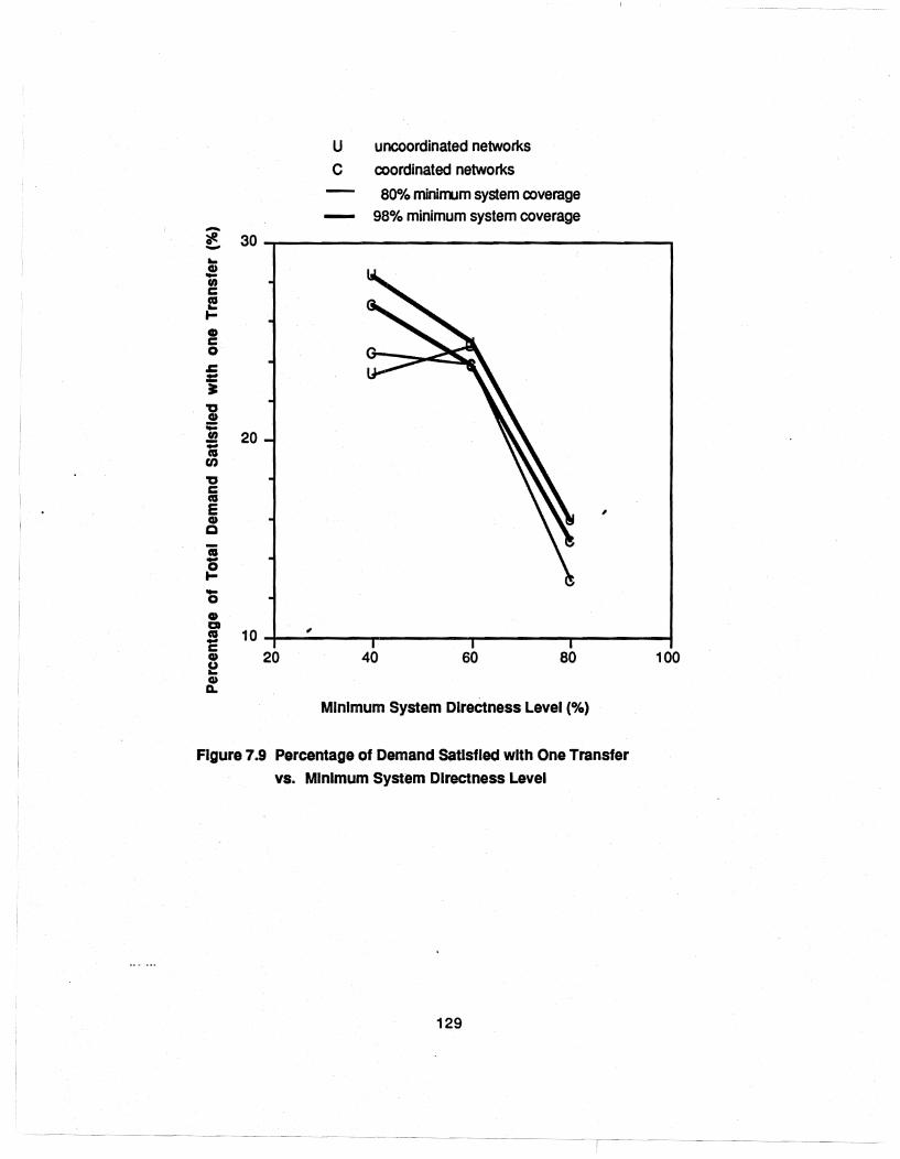
-
U uncoordinated networks
C coordinated networks
80% minimum system coverage - 98% minimum system coverage
-ae 30 ..,...------------------------, -.. .! ." C e I-
! o .t:: -• i ;: ."
1; en '0 c ~
E CD c Ci
~ '0
20
,
CD Q
S 10 ~---'------~------~-------~-------~ c CD 20 ~ CD Q.
40 60 80
Minimum System Directness level (%)
Figure 7.9 Percentage of Demand Satisfied with One Transfer
vs. Minimum System Directness level
129
- -~---------
100
--- - ----1- --- -- ------
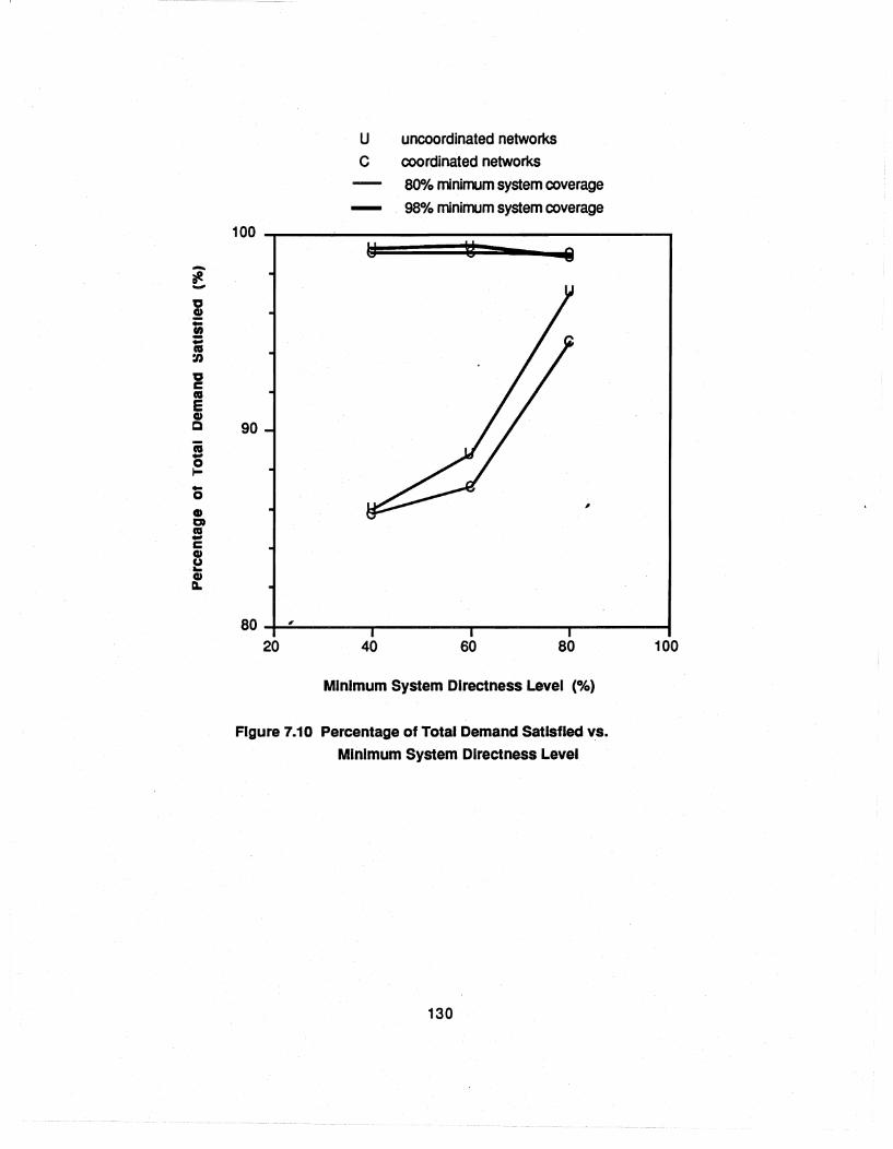
U uncoordinated networks
C coordinated networks
80% minimum system coverage
- 98% minimum system coverage
100 l;j ~ ~ -i'--
0 • ;: ." ;: as :n 0 c as E • Q 90 iii -e .. 0 , • a as -c • () .. • IL
80 '" 20 40 60 80 100
Minimum System Directness Level (%)
Figure 7.10 Percentage of Total Demand Satisfied vs.
Minimum System Directness Level
130

-., CI> -::s .5 E -CD E i= a; > '" .. t-CD U ::c CI> > • .5 ii -0 t-
155000
150000
145000 20
F
V
F
V
F fixed vehicle size
V variable vehicle size
U uncoordinated networks
C coordinated networks
40 60 80
Minimum System Directness Level (%)
Figure 7.11 Total In-Vehicle Travel Time vs. Minimum
System Directness Level for Minimum System
Coverage Level = 80%
131
100

F fixed vehicle size
V variable vehicle size
U uncoordinated networks
C coordinated networks 170000
F -(I) • - V :::s .5. E -• E i= Ci) 160000 F > as V .. .-• c:; :c • > • .5 'ii
~ 150000 ,
20 40 60 80 100
Minimum System Directness Level (%)
Figure 7.12 Total In-Vehicle Travel Time vs. Minimum
System Directness Level for Minimum System
Coverage Level = 98%
132
Total and Average Passenger Qut-of-yehjcle Waning Time' The total out-of-vehicle waiting
times for cases with minimum system coverage of 80% and 98% are presented in Figures 7.15
and 7.16, respectively. In all cases, the coordinated design resulted in better (lower) total out-of
vehicle waiting time because the transfer waiting time was reduced by route coordination at transit
centers. Coordinated Networks yielded higher total out-of-vehicle waiting time savings at the
higher system coverage level. This was expected because a network providing greater coverage
serves more spatially dispersed demand than a network that provides less coverage of the
projected service area. Routes serving spatially dispersed demand generally require low service
frequencies and involve more transfers from and to the low frequency routes. At coordinated
operation centers, more out-of-vehicle waiting time can be saved for passengers transferring to a
lower frequency route than for those transferring to a higher frequency route. Consequently, the
coordinated design is more desirable for areas with spatially dispersed demand than for areas with
high demand density.
Similar conclusions can be reached on the basis of the average passenger out-of-vehicle
waiting time as shown in Figures 7.17 and 7.18. The savings in average out-of-vehicle waiting
time for the coordinated design ranged from 0.1 to 1.4 minutes at the 80% system coverage level-,
and from 0.8 to 1.9 minutes at the 98% coverage level. These savings increased as the minimum
system directness level increased from 40% to 60%, but decreased as the level further increased
from 60% to 80%. At the 40% level, a smaller percentage of routes in the resulting network was
set to low frequencies; 'thus a smaller saving of passenger out-of-vehicle waiting time was
achieved than for case~ at the 60% level. However, at the 80% level, fewer passengers
transferred, yielding smaller total passenger out-of-vehicle waiting time saving.
The use of variable vehicle sizes had meaningful impacts on the out-of-vehicle waiting time
reduction. From the results in Figures 7.17 and 7.18, the average passenger out-of-vehicle
waiting time saved with the variable vehicle size option ranged from 7 to 11 minutes. This saving
resulted mainly from higher service frequencies used with the smaller vehicle sizes.
Total nansler Penatty: Figure 7.19 shows the total transfer penalty for all the networks (each
transfer was considered equivalent to 5 minutes of in-vehicle time). The pattern is similar to the
percentage of total demand satisfied with one transfer shown in Figure 7.9 The uncoordinated
design resulted in a higher total transfer penalty than the coordinated design except at the 80%
level of demand coverage and 40% demand satisfied directly.
133
---- I --c- - ._- - . __ . - -_ .. _- .. - -~ --

F fixed vehicle size
V variable vehicle size
U uncoordinated networks
C coordinated networks
- 31 U) CD -::J .5 E 30 -CD E t= a; 29 > CIS .. t-CD 28 ] U F :c CD > • c 27 .. , CD a c CD 26 ] U) U) CIS V D.
CD a 25 I! , CD 20 40 60 80 100 > C
Minimum System Directness Level (%)
Figure 7.13 Average Passenger In-Vehicle Travel Time vs. Minimum Syst~m Directness Level for Minimum .
System Coverage Level = 80%
134

-0 C» '5 c -E -• E i= CD > t! ... • U :c C» > • c .. C» at C C» 0 0 co Do
• at co .. C» > <
F fixed vehicle size V variable vehicle size
U uncoordinated networks C coordinated networks
30
F
29 V
28 F
V
27 ,
26 20 , 40 60 80 100
Minimum System Directness Level (%)
Figure 7.14 Average Passenger In-Vehicle Travel Time vs. Minimum System Directness Level for Minimum System Coverage Level = 98%
135
-- - ----~- --- - - ----- - - - --- -- -I - - ----;---- -- -- - - -- -- , -
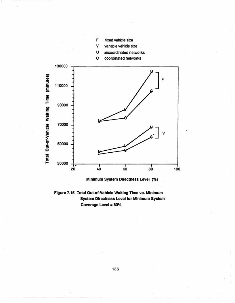
F fixed vehicle size
V variable vehicle size
U uncoordinated networks
C coordinated networks
130000
- } ., CD -;::, c 110000 E -• E j:
90000 lea C
~ as ~
• 70000 U ,J V :c CD > • -0 50000 • -;::, 0
fti -0 f- 30000 ,
20 40 60 80 100
Minimum System Directness Level (%)
Figure 7.15 Total Out-of-Vehlcle Waiting Time vs. Minimum
System Directness Level for Minimum System
Coverage Level = 8001&
136

-(II Cl,) -:s c E -• E t= a c ;: (;
== .! u :c Cl,)
> ,.!. 0 • -:s 0
iii -~
130000
110000
90000
70000
50000
20
F fixed vehicle size
V variable vehicle size
U uncoordinated networks
C coordinated networks
~
40 60
,
80
Minimum System Directness Level (%)
] V
Figure 7.16 Total Out-of-Vehlcle Waiting Time vs. Minimum
System Directness Level for Minimum System
Coverage Level = 98%
137
100

F fixed vehicle size
V variable vehicle size
U uncoordinated networks -." C coordinated networks CD -:::s c E -
] F CD 22 E i= CI c 19 ;:
; CD
£ 16 .c CD > .,:. 0 • 13 -:::s 0 ] .. V CD CI c 10 CD en en • Q.
CD 7 CI t! 20 , 40 60 80 100 CD > C
Minimum System Directness Level (%)
Figure 7.17 Average Passenger Out-of-Vehlcle Wlatlng Time vs.
Minimum System Directness Level for Minimum
System Coverage Level = 80%
138

F fixed vehicle size
V variable vehicle size
- U uncoordinated networks (t) CI)
C coordinated networks -::J .5 E -• 22 E i=
~ at .E
19 -~ • u :c 16 CI)
> .:. 0 • -::J 13 0 J, V .. CI) 01 C CI) 10 rn rn as Q.
• 01 7 as .. CI) 20 40 60 80 100 > , <
Minimum System Directness Level (%)
Figure 7.18 Average Passenger Out-of-Vehlcle Wahlng Time vs.
Minimum System Directness Llevel for Minimum
System Coverage Level = 98%
139
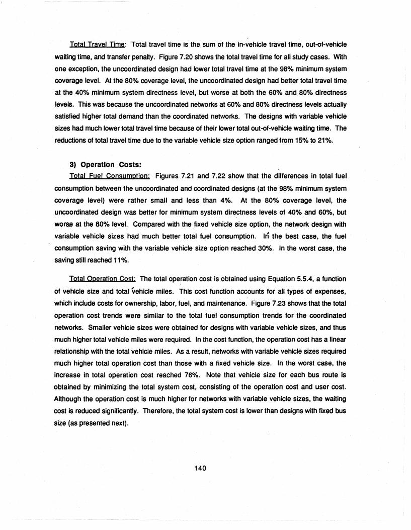
Total Travel Time: Total travel time is the sum of the in-vehicle travel time, out-of-vehicle
waiting time, and transfer penalty. Figure 7.20 shows the total travel time for all study cases. With
one exception, the uncoordinated design had lower total travel time at the 98% minimum system
coverage level. At the 80% coverage level, the·uncoordinated design had. better total travel time
at the 40% minimum system directness level, but worse at both the 60% and 80% directness
levels. This was because the uncoordinated networks at 60% and 80% directness levels actually
satisfied higher total demand than the coordinated networks. The designs with variable vehicle
sizes had much lower total travel time because of their lower total out-of-vehicle waiting time. The
reductions of total travel time due to the variable vehicle size option ranged from 15% to 21 %.
3) Operation Costs:
Total Fuel Consumption: Figures 7.21 and 7.22 show that the differences in total fuel
consumption between the uncoordinated and coordinated designs (at the 98% minimum system
coverage level) were rather small and less than 4%. At the 80% coverage level, the
uncoordinated design was better for minimum system directness levels of 40% and 60%, but
wors.e at the 80% level. Compared with the fixed vehicle size option, the network design with
variable vehicle sizes had much better total fuel consumption. In the best case, the fuel
consumption saving with the variable vehicle size option reached 30%. In the worst case, the
saving still reached 11 %.
Total Operation Cost: The total operation cost is obtained using Equation 5.5.4, a function
of vehicle size and total vehicle miles. This cost function accounts for all types of expenses,
which include costs for ownerShip, labor, fuel, and maintenance. Figure 7.23 shows that the total
operation cost trends were similar to the total fuel consumption trends for the coordinated
networks. Smaller. vehicle sizes were obtained for designs with variable vehicle sizes, and thus
much higher total vehicle miles were required. In the cost function, the operation cost has a linear
relationship with the total vehicle miles. As a result, networks with variable vehicle sizes required
much higher total operation cost than those with a fixed vehicle size. In the worst case, the
increase in total operation cost reached 76%. Note that vehicle size for each bus route is
obtained by minimizing the total system cost, consisting of the operation cost and user cost.
Although the operation cost is much higher for networks with variable vehicle sizes, the waiting
cost is reduced significantly. Therefore, the total system cost is lower than designs with fixed bus
size (as presented next).
140
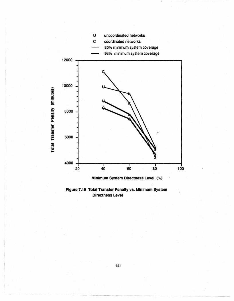
-., CD :; .5 E ->--';; c CD Do .. CD -en c e ... ';; -0 ...
12000
10000
8000
6000
U uncoordinated networks
C coordinated networks
80% minimum system coverage
98% minimum systlem coverage
,
4000 ~--------~------~---------r------~ 20 40 60 80
Minimum System Directness Level (%)
Figure 7.19 Total Transfer Penalty vs. Minimum System Directness Level
141
---- -~- --- -- --
I
100

i -:;, c e -CD e i=
!
300000
280000
260000
240000
220000
80% minimum system coverage - 98% minimum system coverage
F fixed vehicle size
V variable vehicle size
U uncoordinated networks
C coordinated networks
e===o=o ==::e~
~ 200000
180000 20 40 60 80
Minimum System Directness level (%)
Figure 7.20 Total Travel Time vs. Minimum System Directness level
142
l
100

-., c .2 .. a -c 0 :: Co E ::::J en c 0 (J
a; ::::J U. .. -0 I-
F fixed vehicle size
V variable vehicle size
U uncoordinated networks C coordinated networks
450 ~------------------.-----------------,
400
] F
350
300
] V
250
200 ~------~~------~.--------~------~ 20 40 60 80 ,
Minimum System Directness Level (%)
Figure 7.21 Total Fuel Consumption vs. Minimum System Directness Level for Syst1em Coverage Level = 80%
143
------ l---
100

-" c .2 ii Q -c 0 ::: D-E :s " c 0 0 .. :s &I.
a; -f!.
F fixed vehicle size
V variable vehicle size
U uncoordinated networks
C coordinated networks 450 ~----------__ ----------____________ ~
400 ] F
350
300
h~J a v
, 250
,200 ~--------~------~~-------r------~ 20 , 40 60 80 100
Minimum System Directness Level (%)
Figure 7.22 Total Fuel Consumption vs. Minimum System
Directness Level for Minimum System Coverage
Level = 98%
144

-en ... !! '0 " -1;; 0 u c 0 .. e CD a. 0
'ii -0 I-
9000
8000
7000
6000
5000
4000
3000
, 2000
20
- 80% minimum system coverage
- 98% minimum system coverage
F fixed vehicle size
V variable vehicle size
U uncoordinated networks
C coordinated networks
40 60 80
Minimum System Directness Level (%)
Figure 7.23 Total Operation Cost vs. Minimum System
Directness Level
145
----
100

4) Total System Cost:
Figure 7.24 shows that lower total system costs were obtained with the coordinated design
. except for the two cases with the lowest minimum system coverage (40%) and directness levels
(80%). The reductions of total system cost ranged from a few point percentage to 10%. The
results also show that the system cost for variable vehicle size designs was 13% to 17% lower
than fixed vehicle size designs.
Computational Study of the Route Splitting Procedure for Coordinated
Networks
The past section addressed the performance of the RGP and NETAP for different fixed~
route. fixed-schedule service concepts. In the following sections, two modification procedures
are illustrated: route splitting at transit centers and demand responsive service. This section
focuses on the route splitting procedure, intended to improve the effectiveness of the transit
system by splitting unbalanced segments of a route at a transit center so that the route segment
with lower maximum link flow can be operated with a lower frequency of service. Consequently,
operator costs are reduced and higher system utilization can be achieved. However, the route
splitting modification will result in more transfers. This procedure splits routes only at transit
centers so that the waiting time for passengers who are forced to transfer due to route splitting is
reduced through route schedule coordination.
In the previous section, twelve sets of coordinated routes were generated. The route
splitting procedure is tested here on one of the resulting coordinated networks with fixed vehicle , size and values of the minimum system directness and coverage levels of 60% and 98%. The
splitting ratio was defined in Section 6.3.2 as the ratio of the product of the peak load point count
on the proposed two new routes obtained by splitting a route to the square of the peak load point
count on the existing route. The splitting ratio ranges from 0 to 1. A route with a lower splitting
ratio tends to be more amenable to splitting. The sensitivity of the acceptable splitting ratio is
investigated for ratios of 0.2, 0.4, 0.5, 0.6, 0.7, and 0.8. A ratio of zero implies no splitting and
therefore leaves the network unchanged.
Table 7.8 shows the numerical results of the route splitting procedure for different
acceptable splitting ratios. For cases with acceptable splitting ratios up to 0.4, the impacts of the
procedure were not dramatic. In this ratio range, the procedure split only 5 routes and resulted in
the same required fleet size and slight savings in operation cost and fuel consumption. The
percentage of total demand satisfied directly decreased slightly (from 74.31 to 73.13%) and the
percentage of total demand satisfied decreased by only 0.03%. Similarly, the total out-of-vehicle
146
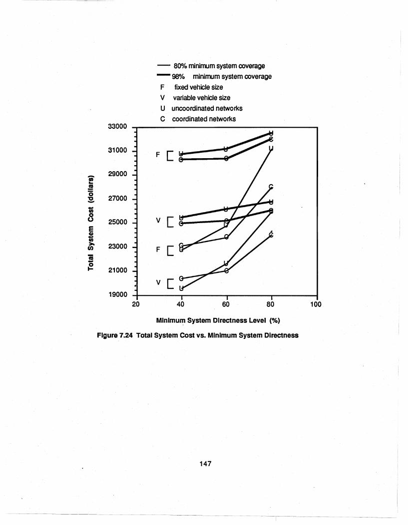
----------
ii -{!
33000
31000
29000
27000
25000
23000
21000
19000 20
- 80% minimum system coverage
- 98% minimum system coverage
F fixed vehicle size
V variable vehicle size
U uncoordinated networks
C coordinated networks
V [
F[
V [
40 60 80
Mlnlmu~ System Directness Level (%)
Figure 7.24 Total System Cost vs. Minimum System Directness
147
100

waiting time increased only 0.6% and the total in-vehicle travel time decreased only 0.3%.
Significant impacts were detected for cases with acceptable splitting ratios greater than 0.4. The
percentage of total demand satisfied directly decreased from 73.13%, to 68.08%, and to 64.70%
as the splitting ralio increased from 0.4, to 0.6, and to 0.8. Correspondingly, the number of routes
split Increased from 5 to 15 and to 22. The total out-of-vehicle waiting time initially worsened
rapidly (approximately 7%) then improved slightly (less than 0.1%) for two reasons: 1) slightly
higher frequencies were set on some of the routes; and 2) some new routes had the same
frequencies as the existing routes; thus each new transferring passenger required a waiting time
of only one half of the transfer time window. The total in-vehicle travel time decreased from
167681 to 165469 and to 164744 minutes. The required fleet size dropped from 97 to 95, and
then to 94 buses. Following the same pattern, the operation cost decreased from $4506 to
$4423, and to $4403; fuel consumption dropped from 389 to 379, and to 378 gallons. The
results indicate that the operation cost can be reduced only up to a certain value of the acceptable
splitting ratio. For a higher ratio, the new routes require the same frequencies of service as the
original routes; and thus no further improvement can be achieved by route splitting.
Figure 7.25 shows each component of user travel time vs. different acceptable splitting
ratioS. The total passenger travel time, which is the sum olthe in-vehicle 'travel time, out-of-vehicle
waiting time, transfer penalty, is worse for higher splitting ratios. The total travel time changes
most for splitting ratios between 0.4 and 0.6. Figure 7.26 shows each component of system cost
vs. the acceptable splitting ra~io. The total system cost increased as the acceptable splitting ratio
increased. Similar pattern as the total passenger travel time was detected. ,
Experiments with the Integrated Bus System Design
At very high demand satisfaction levels (approaching 100% ), the set of routes generated by
the RGP contains many low ridership routes. These routes are operationally uneconomical and
result in ineffective resource allocation. This section investigates the integrated bus system
design concept which uses fixed-route, fixed-schedule service (FRS) for the transit demand that
can be served effectively and demand responsive service (DRS) for the remaining unsatisfied
demand. In the integrated system design procedure, low ridership routes are first discontinued
and the resulting network is then evaluated by the NET AP to identify the unsatisfied demand.
Low ridership routes are identified as those with associated load factor below an acceptable level.
After the unsatisfied demand is identified, the demand responsive service procedure is applied.
The experiments were performed for both uncoordinated and coordinated networks generated in
Section 7.3.2 using the 60% minimum system directness level and the 98% minimum system
148
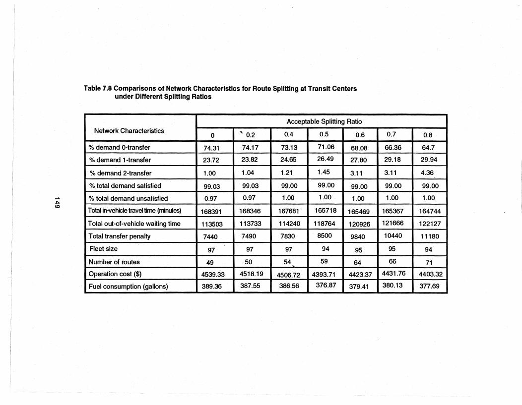
---j
..... .j:>. (0
Table 7.8 Comparisons of Network Characteristics for Route Splitting at Transit Centers under Different Splitting Ratios
Acceptable Splitting Ratio
Network Characteristics 0 ' 0.2 0.4 0.5 0.6
% demand O-transfer 74.31 74.17 73.13 71.06 68.08
% demand l-transfer 23.72 23.82 24.65 26.49 27.80
% demand 2-transfer 1.00 1.04 1.21 1.45 3.11
% total demand satisfied 99.03 99.03 99.00 99.00 99.00
% total demand unsatisfied 0.97 0.97 1.00 1.00 1.00
Total in-vehicle travel time (minutes) 168391 168346 167681 165718 165469
Total out-of-vehicle waiting time 113503 113733 114240 118764 120926
Total transfer penalty 7440 7490 7830 8500 9840
Fleet size 97 97 97 94 95
Number of routes 49 50 54 ~ 59 64
Operation cost ($) 4539.33 4518.19 4506.72 4393.71 4423.37
Fuel consumption (ga"ons) 389.36 387.55 386.56 376.87 379.41
0.7 0.8
66.36 64.7
29.18 29.94
3.11 4.36
99.00 99.00
1.00 1.00
165367 164744
121666 122127
10440 11180
95 94
66 71
4431.76 4403.32
380.13 377.69

0 0.2 0.4 0.5 0.6 0.7 0.8 300000 I I I I I
· Total passenger travel cost ·
250000
0 0.8 . I I I I I -.,
CI) -::s · .5 E - · Total passenger in-vehicle travel time ., CI) 150000 E -t=
: l! t- · Total passenger out-of-vehicle waiting time ~ CI) , '" ::;)
· 100000
I' 12000 -
Total transfer penalty
"l--------6000 ~---------~I-------~I----~I-------~I~-----~I----~
o 02 OA ~5 O~ OJ 0.8
Splitting Ratio
Figure 7.25 User Travel Times vs. Splitting Ratio
150

o 0.2 0.4 0.5 0.6 0.7 0.8
31000
Total system cost
29000
! .!! '0 !!. 27000
Total user cost .. ;; 8 j 25000 '"""-------------------------'
=. en
5000 ~------------------------------------__
4000 - Total operator cost
3000 -+-------rl---.,.....I--~Ir----...;...."'TI---.,.....I--~ o 0.2 0.4 0.5 0.6 0.7 0.8
, Splitting Ratio
Figure 7.26 System Costs vs. Splitting Ratio .
151

coverage level. Each network was tested using two load factor levels (0.4 and 0.8) as cut-off
points for route discontinuation. The performance of the initial networks, the networks after
discontinuing all low ridership routes but before applying the demand responsive service, and the
final integrated networks are reported and compared hereafter.
In Table 7.9, the results of the uncoordinated network are presented. In the initial
uncoordinated network, 10 out of 50 routes had a load factor less than 0.4, and 23 routes had a
load factor less than 0.8. Discontinuation of Iow.ridership routes resulted in lower required fleet
size , operation cost, and fuel consumption. In the case with minimum acceptable load factor
(LFmin) of 0.4, the required fleet size was 92% of that in the initial solution, and the operation cost
and fuel consumption both decreased by 8%. In the case with LFmin = 0.8, the required fleet
size was 86% of that in the initial solution, and the operation cost and fuel consumption both
decreased by 13%. The impacts on the demand satisfaction levels caused by the route
discontinuation were Significant. Compared to the initial solution, the percentage of demand
satisfied directly decreased by 4.1 % for the case with LFmin = 0.4, and 11.1 % for the case with
LFmin - 0.8. As a result, the number of transfers increased by 1.1% and 4.3%, respectively.
Correspondingly, the percentage of total demand satisfied decreased' by 2.9% and 6.6%; the
unsatisfied demand increased from 0.6% to 3.6% and 7.2%. '
After applying the demand responsive service procedure to the unsatisfied demand, the
integrated system satisfied much more demand with only a slight increase in operation cost. For
the cases with the minimum acceptable load factor equal to 0.4 and 0.8, the percentage of total
demand satisfied directly increased 0.59% (from 69.33% to 69.92%) and 1.31% (from 62.31% to , 63.62%), respectively, compared to the network before the DRS procedure. Correspondingly,
the percentage of total demand satisfied increased 0.56% (from 96.95% to 97.51%) and 4.63%
(from 92.81% to 97.44%); the unsatisfied demand decreased from 3.6% to 2.5% and from 7.2%
to 2.6%. Also in comparison with the network before the DRS procedure, the FRS portion had a
slightly larger fleet size (no change for LFmin = 0.4 and one bus increase for LFmin ,. 0.8), and
less than a 1% increase in operation cost and fuel consumption. The 0.4 case required 5 buses
(15 seats) for the demand responsive service. Twelve DRS buses were needed for the case with
LFmin ... 0.8. The results show that the total in-vehicle travel time and out-of-vehicle waiting time
were lower in all modified networks than in the initial network. However, this does not imply that
the modified networks performed better in terms of the above performance measures since each·
network satisfied different levels of demand. Furthermore, the in-vehicle travel time and out-of
vehicle waiting time for passengers using the demand responsive service were neither measured
152

...... 01 VJ
Table 7.9 Network Characteristics for Integrated Bus Systems with Uncoordinated Route Operations
Fixed route and set schedule systems Integrated systems Network characteristics Initial LFrril=0.8 LFrril=0.4 LFrril=0.8
solution LFrril=0.4
% demand O-transfer 7~.44 69.33 62.31 69.92 63.62
% demand Hransfer 24.9 26.07 i
29.25 26.35 31.15
% demand 2-transfer 1.02 1.04 1.24 1.24 2.66
% total demand satisfied 99.38 96.95 92.81 97.51 97.44
% total demand unsatisfied 0;62 3.56 7.19 2.49 2.56
Total in-vehicle-travel time 157632 155688 FRS
151034 156364 156937
Total out-of-vehicle wa~ing time 122765 116616 101670 117056 102008
Total transfer penalty 7800 8140 9180 8200 9590
Fleet size 96 89 83 89 84
Number of routes 50 40 27 40 27
Operation cost 4480.74 4128.13 3881.22 4137.65 3912.41
Fuel consumption 384.34 354.09 332.91 354.91 335.59
Fleet size 0 0 0 5 12
DRS Number of routes 0 0 0 5 12
Total number of DRS trips 0 0 0 62 296

in the procedure nor added to the in-vehicle travel time and out-of-vehicle waiting time shown in
the table. The average passenger in-vehicle travel time and out-of-vehicle waiting time are
expected to be higher in the integrated system because the demand responsive service
generally has more circuitous routes and generates more transfers than the fixed route and set
schedule service.
Table 7.10 shows the results of the coordinated network. The coordinated network after
discontinuing low ridership routes followed the same pattern as the uncoordinated network and
had better fleet size, operation cost, and fuel consumption. The number of routes decreased
from 49 initially to 36 and 28 for the cases with LFmin = 0.4 and LFmin = 0.8, respectively.
Correspondingly,'the fleet size decreased rapidly from 97 to 88 and then slowly to 87 buses. The
operation cost and fuel consumption followed the same pattern as the fleet size and both had a
9.6% reduction for LFmin = 0.4 and a 10.6% reduction for LFmin = 0.8. Differences in the
operation cost (including fleet size, and fuel consumption) between the two load factor cases
were insignificant because of the frequency setting procedure in the coordinated design. Since
the service frequencies for all coordinated routes need to be set to the same or multiple Integer
values, the operation cost is affected by the frequency setting procedure. Thus, the operation
cost in the coordinated design case may not change as much as in tne uncoordinated design
case. The demand satisfaction levels were worse in the coordinated networks after the route
discontinuation was applied. The percentage of total demand satisfied directly for LFmin = 0.4 and
0.8 decreased by 3.9% and 8.2%, respectively. The percentage of total demand satisfied
decreased by 2.0% and 6.1%; the percentage of total unsatisfied demand increased from 1% to , 3% and 7% for the two minimum acceptable load factors.
In comparison with the networks before the DRS procedure, the integrated coordinated
system obtained better demand satisfaction levels with no increase in fleet size for the FRS
portion. The results show that the integrated system satisfied higher percentages of total
demand directly (0.44% more for the case with LFmin = 0.4 and 1.17% more for the case with
LFmin - 0.8). The percentages of total demand satisfied were increased by 0.93% and 4.04% for
the above two cases. The percentages of total unsatisfied demand for the above two cases were
lower (2.04% vs. 2.97% and 3.01% vs. 7.05%). Four buses were required to operate the
demand responsive service for LFmin z: 0.4; 11 buses were needed for the case with LFmin = 0.8.
Similar to the uncoordinated networks, the modified coordinated networks had lower total in
vehicle travel time and total out-of-vehicle waiting time. However, when comparing these two
performance measures, the factors described for the uncoordinated case need to be considered
here as well.
154
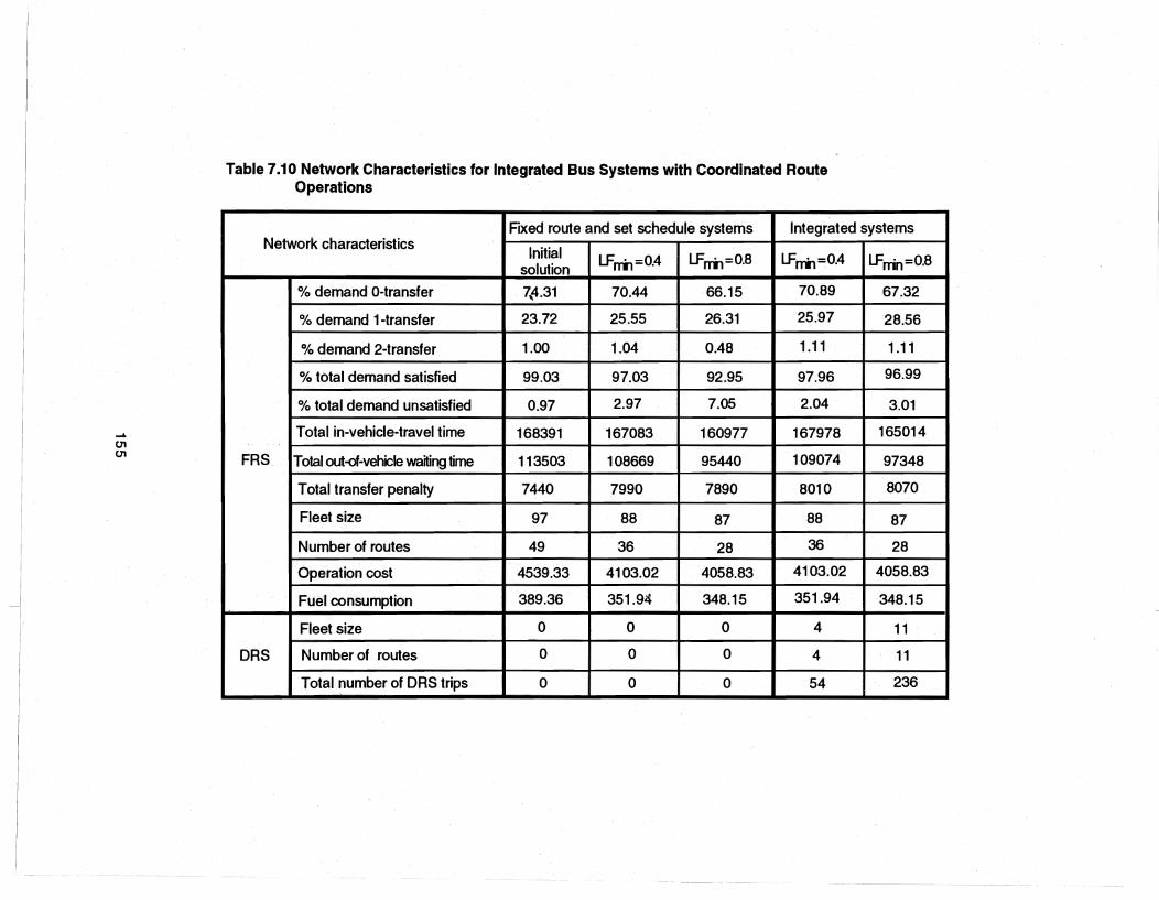
01 01
Table 7.10 Network Characteristics for Integrated Bus Systems with Coordinated Route Operations
Fixed route and set schedule systems Integrated systems Network characteristics
Initial solution LFrri1=0.4 LFrri1=0.8 LFni1=0.4 LFrrin=0.8
% demand O-transfer 7~.31 70.44 66.15 70.89 67.32
% demand 1-transfer 23.72 25.55 26.31 25.97 28.56
% demand 2-transfer 1.00 1.04 0.48 1.11 1.11
% total demand satisfied 99.03 97.03 92.95 97.96 96.99
% total demand unsatisfied 0.97 2.97 7.05 2.04 3.01
Total in-vehicle-travel time 168391 167083 160977 167978 165014
FRS Total out-of-vehicle wa~ing time 113503 108669 95440 109074 97348
Total transfer penalty 7440 7990 7890 8010 8070
Fleet size 97 88 87 88 87
Number of routes 49 36 28 36 28
Operation cost 4539.33 4103.02 4058.83 4103.02 4058.83
Fuel consumption 389.36 351.9~ 348.15 351.94 348.15
Fleet size 0 0 0 4 11
DRS Number of routes 0 0 0 4 11
Total number of DRS trips 0 0 0 54 236
Summary of Tests on the Austin Transit Network
The previous sections of this chapter focused on the tests of the design procedures and
alternative design concepts in the solution framework. These tests were conducted with data
generated from the transit system of Austin, Texas. The TCSP was tested under two application
strategies and six selected combinations of minimum system coverage and directness levels.
Twelve sets of transit centers were generated in the TCSP tests. Thirty-six RGP runs and an
equal number of NETAP runs were executed to investigate the performance of design
alternatives with and without route coordination and variable vehicle sizes. The same six
combinations of minimum system coverage and directness levels were used as in the test of the
TCSP. The route splitting procedure for improving the effectiveness of coordinated networks
was tested. The sensitivity of the procedure to the acceptable splitting ratio was investigated.
Finally, the integrated bus system concept was tested on a coordinated network and
uncoordinated network. This included the test of the demand responsive service procedure.
Analysis of the test results leads to the following conclusions:
1) The TCSP generates robust solutions for cases using different application strategies and
different combinations of minimum system coverage and directness levels.
2) The coordinated design results in lower total out-of-vehicle waiting tfme and total system cost.
Since the coordinated design incurs in-vehicle waiting time for non-transferring passengers at
transit centers, the in-vehicle travel time and total passenger travel time are higher. Neither the
coordinated design nor the uncoordinated design appear to consistently outperform the
others in terms of the Veet size, total operation cost, or fuel consumption. With respect to out
of-vehicle waiting time, the coordinated service concept is more suitable for designs that satisfy
high minimum system coverage levels. The coordinated service concept may not be
particularly advantageous for designs that satisfy high system directness levels since only
limited waiting time savings can be achieved with such a design.
3) The network deSign with the variable vehicle size option has much better total out-of-vehicle
waiting time, total travel time, total system cost and fuel consumption, and slightly better in
vehicle travel time. However, using the variable vehicle size option requires much higher total
operation cost.
4) The route splitting procedure for the coordinated network improves network effectiveness and
results in lower fleet size, operation cost and f!Jel consumption. In addition, the procedure
reduces in-vehicle travel time. However, route splitting causes more passengers to transfer
and thus reduces the percentage of total demand satisfied directly and increases the total
waiting time. Sensitivity analysis of the acceptable splitting ratio shows that the impacts of the
156

splitting become significant as the ratio reaches a certain value (0.4 in the study case).
Improvements in system effectiveness appear to be obtainable only for ratios up to a certain
value (0.6 in the study case).
5) The integrated bus system results in lower fleet size, operation cost and fuel consumption.
However, the negative impacts on the demand satisfaction levels are significant. Operators
should investigate the trade-offs so as to obtain a more effective transit system with acceptable
reductions in levels of service.
,
,
157

CHAPTER 8. CONCLUSIONS AND RECOMMENDATIONS
The primary objective of this study is to develop and test computer-based procedures which
incorporate aHernative service concepts into the design of bus transit route networks. This work
complements and extends the initial solution approach to the bus transit network design problem
presented by Baaj and Mahmassani (1991), which was limited to the design of conventional fixed
route, fixed-schedule, fixed vehicle size, and uncoordinated bus transit systems. Conventional
service is generally suitable for areas with high and dense transit demand. For areas with medium,
low, or spatially dispersed demand patterns of the type prevailing in most U.S. urban areas,
alternative service concepts including coordinated systems, variable vehicle sizes, and demand
responsive service have been used to a limited degree with generally positive resuHs. The focus
of this study is the development of a bus transit design model which incorporates the above
service concepts.
In the next section, the principal features of the design procedures are reviewed, followed by
a summary of conclusions from the computational tests. Section 8.2 presents a brief discussion
of possible directions for further research. ,
SUMMARY AND CONCLUSION
The bus transit network design problem addressed in this report is to construct a set of bus·
routes and determine the associated service frequencies and vehicle sizes. Several sources of
complexity were recognized by Baaj (1990) including difficulty of formulating the problem; non-, linearity andnon-convexity of the mathematical formulation; inherent combinatorial complexity of
the problem; muHi-objective nature of the problem; and spatial layout of routes for solving such a
bus network design problem. These inherent complexities preclude finding a unique optimal
solution using optimization formulations. This study is an attempt to find good and efficient
solutions to the bus transit network design problem via AI search heuristic approaches.
Previous approaches to the transit network design were either OR heuristic approaches with
limited applicability, or practical guidelines and ad hoc procedures reflecting important current
practice, but not sufficient on their own. The shortcomings of previous approaches .include failure
to address the inherent multi-objective nature of the transit network design problem, limited
responsiveness to the demand pattern in the route layout, failure to incorporate aHernative design
concepts, and failure to consider service planning guidelines and professional judgment of transit
planners. The solution approach, which has evolved from Baaj and Mahmassani's algOrithm,
includes the following major features: 1) an AI search heuristic for transit route generation and
158
improvement, 2) a transit network evaluation model to compute a variety of system performance
measures, and 3) systematic use of context-specific knowledge to guide the search technique.
Alternative design concepts and features oriented towards the kind of land use and transit
demand pattern found in most U.S. cities are incorporated to provide transit planners with
additional service design dimensions. Additional system performance measures are computed to
provide useful information to operators so that trade-offs between conflict objectives can be
clearly addressed.
The solution approach consists of four algorithmic procedures; The route generation
procedure (RGP) constructs sets of bus routes for deSigns with or without the transit center
concept. The network evaluation procedure (NETAP) determines route service frequencies and
vehicle sizes and evaluates transit systems for both coordinated and uncoordinated designs. The
transit center selection procedure (TCSP) identifies candidate sets of transit centers when the
network is to be configured around the transit center concept. The network improvement
procedures (NIP) applies modifications to the set 'of routes generated by the RGP to improve
performance from the user's or operator's perspective.
Numerical experiments were performed to test the solution approach on a benchmark
problem. The results showed that networks generated by the RGP'around the transit center
concept outperformed the solutions of Mandl's and Baaj and Mahmassani's algorithm. Numerical
experiments on data for the transit system of Austin, Texas, were also performed to test the
design procedures and investigate the performance of alternative designs. The TCSP was tested
based on two application strategies and six selected combinations of demand satisfaction levels. , The tests indicated that the TCSP generated consistent results in all study cases. Transit centers
generated from the TCSP were either major activity centers or transit nodes within major
communities in the suburban areas. The RGP and NETAP were tested using four design
alternatives under six combinations of demand satisfaction levels. The tests compared the
performance of coordinated vs. uncoordinated networks. The tests also investigated the
performance of networks with the variable vehicle sizes vs. fixed vehicle size. The numerical
results showed that 1) the coordinated design resulted in better demand satisfaction levels. total
out-of-vehiclewaiting time, and total system cost, but worse total in-vehicle travel time and total
travel time because additional in-vehicle waiting time was generated by the route coordination, 2)
designs with variable vehicle sizes greatly reduced the total system cost, fuel consumption, and
out-of-vehiclewaiting time, but increased the operation cost. Two possible NIP modifications
were tested. The procedure that splits routes at transit centers reduced the required operational
resources, but the levels of demand satisfaction were decreased, The demand responsive
159

service procedure resulted in significant savings of operating resources and much lower
reductions in the levels of demand satisfaction compared to outright route discontinuation.
The principal unique features of this work, which define its contribution, are:
1) A computer-based route generation procedure which is superior to other route generation
algorithms by incorporating the transit center concept to provide good transfer opportunities at
transit centers and fast and direct service between transit centers.
2) A transit network analysis procedure with the following important features:
i) It incorporates a trip assignment procedure which assigns trips for both uncoordinated and
coordinated networks. This enables the evaluation and design of timed-transfer bus
system designs.
ii) It computes system performance measures reflecting service quality, user costs, and
operator costs.
iii) It can be used as a sensitivity analysis tOol for system performance measures and a variety of
variables and parameters such as route configuration, route frequency, bus seating
capacity, transfer penalty, maximum allowable route load factor, timed-transfer window,
waiting time value, in-vehicle travel time value, and operation cost coefficients.
3) A vehicle sizing procedure which provides the transit operator with an additional choice
dimension to design the service configuration to better meet user needs and desired service
level.
4) A transit center selection procedure which identifies suitable transit centers to support the
implementation of timed-transfer design and demand responsive service. , 5) A computer-based procedure to identify suitable service areas and the corresponding transit
center for the provision of demand responsive service. The procedure enables the design of
an integrated bus system that serves high density demand with fixed-route and fixed-schedule
service and low density demand with demand responsive service.
FUTURE RESEARCH
In the present verSion, the route generation procedure is a long range planning tool which
generates a new set of routes for a given projected service area. For the route generation
procedure to support short or medium range planning, it needs to be capable of modifying or
replacing a subset of routes of the existing transit system. This is extremely important because
any transit planning tool intended to be used in practice should offer this capability.
The ability to display the results graphically is "extremely important to any network design
problem. As shown in the output for the RGP and NETAP, the set of routes was presented in the
160

fonn of a Ust of transit nodes, which cannot give transit planners an instant pidure of route layouts.
It would be extremely useful if the transit planner could delineate the resulting route network and
develop a 'feer for the performance of the route design, by means of the graphic display ability. In
addition, network descriptors computed by the NETAP could be made explicit using graphic
display technology so that transit operators would quickly notice the sensitivity of the resulting
solutions to different. user input parameters.
The solution approach requires further testing on different transit networks and their
corresponding transit demand matrices. The solution approach provides alternative design
features that are applicable to different demand levels and spatial distributions. Therefore, it
would be extremely valuable to perform systematic tests of alternative service deSign concepts
under different demand patterns to ascertain the conditions that determine their success.
Lastly, incorporating other service choice dimensions which could improve the performance
of bus transit systems will make the solution approach more versatile. One example is express
bus service that serves two terminal nodes non-stop or with limited stops. In addition, application
of the solution approach in other urban transportation network problems should be investigated,
especially in integratea bus and rail systems. The integrated bus and rail system is a common
combination in urban transit systems. Urban rail systems usually serve as trunk or main lines
interconneding the various transit centers. They usually have fewer routes than bus networks,
higher service frequencies, larger passenger capacities, and more transferring activity among
routes. They are essentially the same as the express bus service with higher vehicle seating
capacity and more reliable service schedules. Therefore, with some minor modifications, the , solution approach would be applicable in this context.
161

Appendix A Node Selection and Insertion Strategies
Four different node selection and insertion strategies are considered:
a) 1-Link, Maximum Demand Insertion (MD)
b) 1-Link, Maximum Demand per Minimum Time Insertion (MDMT)
c) 1-Link, Maximum Demand per Minimum Route Length Increase Insertion MDML)
d) 1-Unk, Maximum Demand per Minimum Cost Insertion (MDMC)
Each of these strategies is discussed in turn hereinafter.
l-Llnk, Maximum pemand Insertion (MOl
Step I) (Generation of Feasible Insertion Nodes). For a given route ro under expansion, find
the set of feasible insertion nodes. If this set is empty, terminate the route
expansion, otherwise proceed to Step 2.
Step 2) (Node Selection and Insertion). Select node i whose DDSi is the maximum and
insert it in rO (call the new route r1). DDSi is the increase in the network's total
demand satisfied directly as a result of inserting node i in route rO (considering only
the yet unsatisfied node pairs). ,
Step 3) (Termination Test). If the new route r1 is feasible, (i.e. both r1's capacity and length
are acceptable) then set rO = r1 and return to Step 1. Otherwise, terminate the route
expansion process and return rOo
l-Llnk, MaxImum pemand per Minimum TIme Insertion (MOMT)
Same as MD heuristic, but replace Step 2 by the following: Step 2) (Selection and Insertion). Select node i whose{DDS/DTinvh is a maxilTlJm and insert
it. DDS is as defined in the MD heuristic while DTinv is the corresponding increase
in the total in-vehicle travel time.
l-Llnk, Maximum Demand per Minimum Route Length Increase Insertion (MPML)
Same as MD heuristic, but replace Step 2 by the following: Step 2) (Selection and Insertion). Select node i whose {DDS 1DTrO}i is a maximum and insert
it. DDS is as defined in the MD heuristic while DTra is the corresponding increase in
route ro's length (i.e. the difference in the round trip times of ra and r1).
,-Link. Maximum pemand per Minimum Cost Insertion (MDMC)
Same as MD heuristic, but replace Step 2 by the following:
162

Step 2) (Selection and Insertion). Select node i whose {DDS I [C1(DTinv) + C2(DTrO))i} is a
maximum and insert it. DDS is as defined in the MD heuristic while DTinv and DT ro
are as defined in the MDMT and MDML heuristics. respectively. CI and C2 are
constants that express different tradeoffs between the proxies of the user and
operator costs. Currently. they are chosen in such a way that both user and
operator cost are weighted equally.
,
,
163
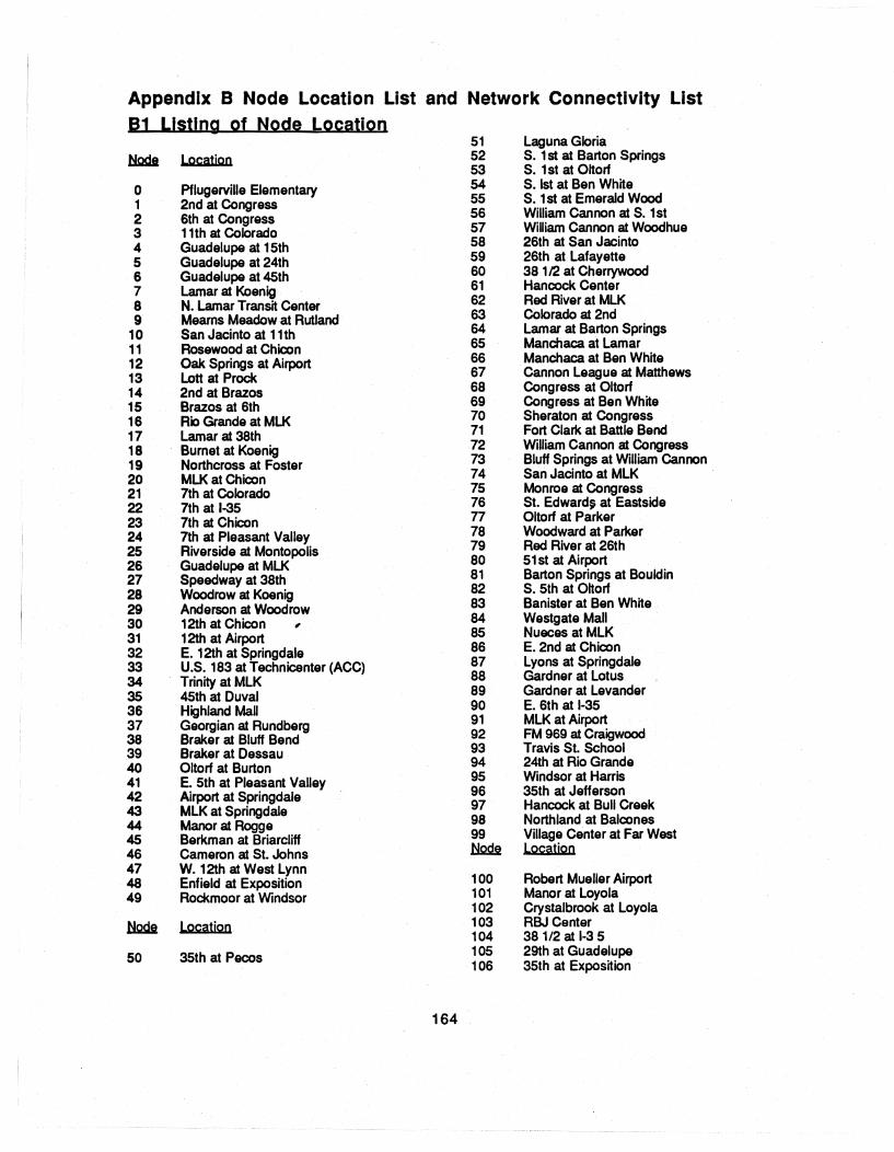
Appendix B Node Location List and Network Connectivity List B1 Listing of Node Location
51 Laguna Gloria tjgda Location 52 S. 1 st at Barton Springs
53 S. 1 st at Oltorf
0 Pflugerville Elementary 54 S. 1st at Ben White
1 2nd at Congress 55 S. 1 st at Emerald Wood
2 6th at Congress 56 William Cannon at S. 1st
3 11th at Colorado 57 William Cannon at Woodhue
4 Guadelupe at 15th 58 26th at San Jacinto
5 Guadelupe at 24th 59 26th at Lafayette
6 Guadelupe at 45th 60 38 112 at Cherrywood
7 Lamar at Koenig 61 Hancock Center
8 N. Lamar Transit Center 62 Red River at MLK
9 Mearns Meadow at Rutland 63 Colorado at 2nd
10 San Jacinto at 11 th 64 Lamar at Barton Springs
11 Rosewood at Chicon 65 Manchaca at Lamar
12 Oak Springs at Airport 66 Manchaca at Ben White
13 Lott at Prock 67 Cannon League at Matthews
14 2nd at Brazos 68 Congress at Oltorf
15 Brazos at 6th 69 Congress at Ben White
16 Rio Grande at MLK 70 Sheraton at Congress
17 Lamar at 38th 71 Fort Clark at Battle Bend
18 Burnet at Koenig 72 William Cannon at Congress
19 Northcross at Foster 73 Bluff Springs at William Cannon
20 MLK at Chicon 74 San Jacinto at MLK
21 7th at Colorado 75 Monroe at Congress
22 7th at 1-35 76 St. Edward~ at Eastside
23 7th at Chicon n Oltorf at Parker
24 7th at Pleasant Valley 78 Woodward at Parker
25 Riverside at Montopolis 79 Red River at 26th
26 Guadelupe at MLK 80 51st at Airport
27 Speedway at 38th 81 Barton Springs at Bouldin
28 Woodrow at Koenig 82 S. 5th at Oltorf
29 Anderson at Woodrow 83 Banister at Ben White
30 12th at Chicon , 84 Westgate Mall
31 12th at Airport 85 Nueces at MLK
32 E. 12th at Springdale 86 E. 2nd at Chicon
33 U.S. 183 at Technicenter (ACC) 87 Lyons at Springdale
34 Trinity at MLK 88 Gardner at Lotus
35 45th at Duval 89 Gardner at Levander
36 Highland Mall 90 E. 6th at 1-35
37 Georgian at Rundberg 91 MLK at Airport
38 Braker at Bluff Bend 92 FM 969 at Craigwood
39 Braker at Dessau 93 Travis St. School
40 Oltorf at Burton 94 24th at Rio Grande
41 E. 5th at Pleasant Valley 95 Windsor at Harris
42 Airport at Springdale 96 35th at Jefferson
43 MLK at Springdale 97 Hancock at Bull Creek
44 Manor at Rogge 98 Northland at Balcones
45 Berkman at Briarcliff 99 Village Center at Far West
46 Cameron at St. Johns ~ Location
47 W. 12th at West Lynn 48 Enfield at Exposition 100 Robert Mueller Airport
49 Rockmoor at Windsor 101 Manor at Loyola 102 Crystal brook at Loyola
l:k2di Location 103 RBJ Center 104 38 1/2 at 1-3 5
50 35th at Pecos 105 29th at Guadelupe 106 35th at Exposition
164
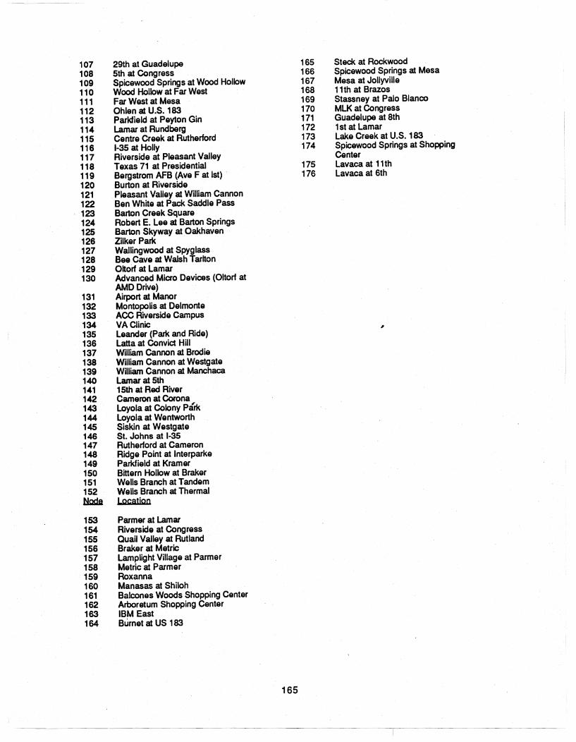
107 108 109 110 111 112 113 114 115 116 117 118 119 120 121 122 123 124 125 126 127 128 129 130
131 132 133 134 135 136 137 138 139 140 141 142 143 144 145 146 147 148 149 150 151 152 ~
29th at Guadelupe 5th at Congress Spicewood Springs at Wood Hollow Wood Hollow at Far West Far West at Mesa Ohlen at U.S. 183 Parkfield at Peyton Gin Lamar at Rundberg Centre Creek at Rutherford 1-35 at Holly Riverside at Pleasant Valley Texas 71 at Presidential Bergstrom AFB (Ave Fat 1st) Burton at Riverside Pleasant Valley at William Cannon Ben White at Pack Saddle Pass Barton Creek Square Robert E. Lee at Barton Springs Barton Skyway atOakhaven ZUker Park Walling wood at Spyglass Bee Cave at Walsh Tarlton Oltorf at Lamar Advanced Micro Devices (Oltorf at AMD Drive) Airport at Manor Montopolis at Delmonte Ace Riverside Campus VA Clinic Leander (Park and Ride) Latta at Convid Hill William Cannon at Brodie William Cannon at Westgate William Cannon at Manchaca Lamar at 5th 15th at Red River Cameron at Corona Loyola at Colony Park Loyola at Wentworth Siskin at Westgate St. Johns at 1-35 Rutherford at Cameron Ridge Point at Interparke Parkfield at Kramer Bittern Hollow at Braker Wells Branch at Tandem Wells Branch at Thermal Locatipn
153 Parmer at Lamar 154 Riverside at Congress 155 Quail Valley at Rutland 156 Braker at Metric 157 Lamplight Village at Parmer 158 Metric at Parmer 159 Roxanna 160 Manasas at Shiloh 161 Balcones Woods Shopping Center 162 Arboretum Shopping Center 163 IBM East 164 Burnet at US 183
165
165 166 167 168 169 170 171 172 173 174
175 176
Steck at Rockwood Spicewood Springs at Mesa Mesa at Jollyville 11th at Brazos Stassney at Palo Blanco MLK at Congress Guadelupe at 8th 1st at Lamar Lake Creek at U.S. 183 Spicewood Springs at Shopping Center Lavaca at 11 th Lavaca at 6th
,
---, -- -

82 Network Connectlylty List
(setf ·CONNECTIVITY-L1ST*' '«0 «3749.0) (38 42.0) (11558.1) (146 56.1) (147 57.05) (148 63.35) (153 30.45)))
(1 «140.35) (520.75) (63 0.35) (8717.5) (108 1.25) (116 4.25) (1542.45)(1724.65))) (2 «3 2.75) (15 0.4)(210.75) (22 2.95) (108 0.4) (168 2.9) (176 0.8))) (3 «22.75)(211.35) (168 0.85) (1711.25) (115 0.35))) (4 «103.4) (162.3)(261.45) (34 3.5)(47 5.25) (743.5) (852.15)(1413.75) (1702.4) (171 2.5) (1751.8))) (5 «262.15) (344.9) (852.1) (941.15) (105 2.7))) (6 «75.65) (17 4.1)(274.65) (289.05) (35 2.85) (97 9.65) (1056.1))) (7 «65.65) (89.65) (28 2.5) (2910.5) (35 9.1) (36 5.9) (14610.15))) (8 «7 9.65) (28 10.05) (293.5) (369.0) (377.0) (3821.0) (1125.6)(1138.1) (114 8.95) (115 13.0) (146
7.2) (147 11 .• 25) (148 13.9))) (9 «3812.9) (1134.2) (1142.45) (1499.0) (153 13.6) (1557.5))) (10 «11 7.05) (143.4) (15 2.0) (22 3.5) (30 6.95) (34 3.2) (742.15)(86 6.9) (903.5) (103 6.55) (10410.5)
(1167.2) (1412.35) (1680.4)(1712.95))) (11 «107.05) (127.35) (232.65) (246.0) (30 1.4) (42 9.15) (877.9)(906.15))) (12 «11 7.35) (13 7.5) (247.0) (311.45) (323.4) (42 2.85) (874.9))) (13 «12 7.5) (326.55)(42 7.8))) (14 «1 0.35) (10 3.4) (15 1.2) (22 3.85) (34 6.65) (90 3.4) (103 7.5)(108 1.35) (172 5.05))) (15 «2 0.4) (141.2) (22 2.85) (103 8.6) (108 0.1) (168 1.8))) (16 «4 2.3) (85 0.4) (94 1.9) (95 5.1) (115 4.15))) (17 «64.7) (1810.1) (273.3) (289.75) (958.15) (962.95) (9710.5)(1054.75))) (18 «1710.1) (1911.15) (282.85) (977.8) (984.6))) (19 «1811.15) (295.95) (9716.85) (9812.6) (109 4.25) (112 9.55)(164 9.4) (165 3.95))) (20 «302.1) (591.75) (623.6) (915.6) (1316.15))) (21 «20.75) (31.35) (22 2.95) (631.8) (140 3.95) (171 0.8))) (22 «103.5) (143.85) (15 2.85) (21 2.95) (234.0) (305.1) (34 5.6)(62 4.8) (96 0.4) (10410.5) (141 3.95)
(168 3.45))) (23 «11 2.65) (244.7) (41 4.4) (861.1) (904.4))) (24 «127.0) (411.2)- (42 7.35) (874.55) (89 7.2) (13211.2))) (25 «11 6.0) (40 12.05) (117 12.1) (118 16.1) (130 12.15) (1327.9)(133 6.35)(1343.95))) (26 «41.45) (5
2.15) (85 0.75) (170 1.1))) (27 «64.65)(173.3) (354.5) (584.4) (614.4) (104 4.8) (105 4.25)(1707.2))) (28 «69.05) (72.5) (810.05) (17 9.75) (182.85) (298.05) (367.45)(975.25))) (29 «710.5) (83.5) (19 5.t5) (28 8.05) (3610.0) (112 6.1)(164 8.55))) (30 «10 6.95) (111.4) (20 2.1) (22 5.1) (31 6.9)(141 4.4))) (31 «121.45) (30 6.9) (324.75) (91 2.25) (1004.9))) (32 «12 3.4) (13 6.55) (31 4.75) (3314.3) (42 4.2) (43 3.6) (929.2) (100 6.3))) (33 «32 14.3) (43 7.9) (887.2) (92 4.1) (101 12.25) (10211.05)(148 21.35))) (34 «5 4.9) (14 6.65) (22 5.6) (583.6) (62 0.1) (74 0.35))) (35 «6 2.85) (7 9.1) (27 4.5) (36 13.0) (58 6.05) (61 3.1)(80 4.2)(104 3.15))) (36 «75.9) (89.0) (2910.0) (3513.0) (3723.45) (4511.2) (468.4)(802.3) (1427.1)(146 9.8) (14818.9))) (37 «8 7.0) (3623.45) (3812.65) (3914.0) (1141.55) (11514.65)(14611.9) (14711.9) (14818.2) (0
49.0))) (38 «8 21.0) (9 12.9) (3712.65) (393.65) (11412.05) (115 19.6)(14618.9)(14715.25) (14817.5) (149
8.75) (153 14.0) (042.0))) (39 «3714.0) (38 3.65) (11514.0)(14715.6) (14816.1) (15320.65))) (40 «25 12.05) (771.15) (1175.5) (1203.1) (1306.7))) (41 «234.4) (241.2) (864.8) (875.25) (103 7.35) (117 8.1) (120 9.45)(132 8.75))) (42 «11 9.15) (122.85) (137.8) (247.35) (324.2) (871.75) (88 8.25)(89 7.0) (1328.6))) (43 «323.6) (33 7.9) (44 8.55) (91 7.35) (925.95) (100 6.5) (101 8.75)(10212.95))) (44 «43 8.55) (45 7.5) (100 10.35) (1014.95))) (45 «3611.2) (44 7.5) (46 5.65) (101 10.65) (142 4.6) (148 10.5))) (46 «36 8.4) (45 5.65) (101 15.4) (115 6.65) (1425.95) (146 5.8)(1474.5) (148 10.15))) (47 «4 5.25) (48 7.0) (954.2) (107 7.55) (108 8.4) (126 8.75) (1405.1)(171 6.15) (175 30.95) (1767.6))) (48 «47 7.0) (49 6.65) (95 6.15) (9611.55) (106 9.15) (107 2.9))) . (49 «486.65) (SO 7.85) (106 9.95))) (50 «49 7.85) (51 10.15) (97 13.3) (98 10.5) (1061.45)))
166
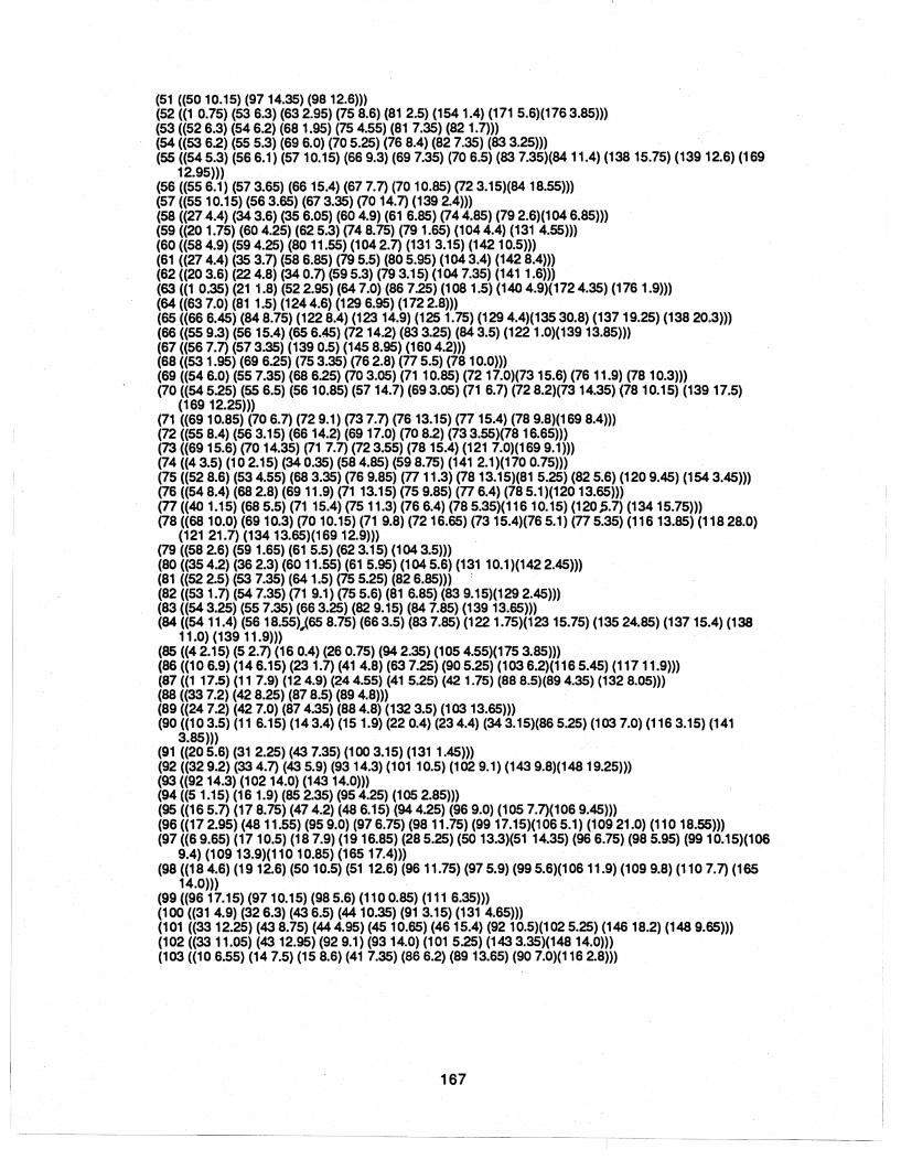
(51 «5010.15) (9714.35) (9812.6))) (52 «1 0.75) (53 6.3) (632.95) (75 8.6) (81 2.5) (1541.4) (171 5.6)(1763.85))) (53 «52 6.3) (546.2) (68 1.95) (754.55) (81 7.35) (82 1.7))) (54 «53 6.2) (55 5.3) (69 6.0) (705.25) (76 8.4) (827.35) (83 3.25))) (55 «545.3) (566.1) (57 10.15) (669.3) (69 7.35) (706.5) (83 7.35)(84 11.4)(138 15.75) (139 12.6) (169
12.95))) (56 «55 6.1) (573.65) (66 15.4) (677.7) (70 10.85) (72 3.15)(84 18.55))) (57 «5510.15) (56 3.65) (673.35) (70 14.7) (139 2.4))) (58 «274.4) (34 3.6) (356.05) (60 4.9) (61 6.85) (744.85) (792.6)(104 6.85))) (59 «20 1.75) (604.25) (62 5.3) (748.75) (791.65) (1044.4) (1314.55))) (60 «584.9) (594.25) (80 11.55) (104 2.7) (131 3.15) (142 10.5))) (61 «274.4) (35 3.7) (586.85) (795.5) (805.95) (104 3.4) (1428.4))) (62 «20 3.6) (22 4.8) (34 0.7) (595.3) (79 3.15) (104 7.35) (141 1.6))) (63 «1 0.35) (21 1.8) (522.95) (64 7.0) (86 7.25) (108 1.5) (140 4.9)(172 4.35) (176 1.9») (64 «63 7.0) (81 1.5) (1244.6) (129 6.95) (1722.8))) (65 «66 6.45) (848.75) (1228.4) (123 14.9) (125 1.75) (129 4.4)(135 30.8) (137 19.25) (138 20.3))) (66 «559.3) (56 15.4) (65 6.45) (72 14.2) (83 3.25) (84 3.5) (122 1.0)(139 13.85))) (67 «56 7.7) (573.35)(1390.5) (145 8.95) (1604.2))) (68 «53 1.95) (69 6.25) (753.35) (762.8) (77 5.5) (78 10.0))) (69 «54 6.0) (557.35) (68 6.25) (703.05) (71 10.85) (72 17.0)(73 15.6) (76 11.9) (78 10.3))) (70 «54 5.25) (55 6.5) (56 10.85) (57 14.7) (693.05) (71 6.7) (728.2)(73 14.35) (78 10.15) (139 17.5)
(169 12.25))) (71 «6910.85) (706.7) (72 9.1) (737.7) (7613.15) (7715.4) (789.8)(1698.4))) (72 «55 8.4) (563.15) (66 14.2) (69 17.0) (70 8.2) (733.55)(7816.65))) (73 «6915.6) (70 14.35) (71 7.7) (723.55) (7815.4) (1217.0)(169 9.1))) (74 «4 3.5) (102.15) (34 0.35) (584.85) (598.75) (141 2.1 )(170 0.75}}) (75 «52 8.6) (534.55) (68 3.35) (76 9.85) (77 11.3) (78 13.15)(81 5.25) (825.6) (1209.45)(154 3.45))) (76 «548.4) (682.8) (69 11.9) (71 13.15) (75 9.85) (77 6.4) (785.1 )(12013.65))) (77 «40 1.15) (68 5.5) (71 15.4) (75 11.3) (76 6.4) (78 5.35)( 116 1 0.15) (120:;.7) (134 15.75))) (78 «68 1 0.0) (69 10.3) (70 10.15) (71 9.8) (72 16.65) (73 15.4)(76 5.1) (77 5.35) (116 13.85) (118 28.0)
(12121.7) (13413.65}(16912.9))) (79 «58 2.6) (59 1.65) (61 5.5) (62 3.15) (104 3.5))) (80 «354.2) (362.3) (60 11.55) (61 5.95) (1045.6) (131 10.1 )(1422.45))) (81 «522.5) (53 7.35) (641.5) (755.25) (826.85))) . (82 «53 1.7) (547.35) (71 9.1) (75 5.6) (81 6.85) (83 9.15)(1292.45))) (83 «54 3.25) (557.35) (663.25) (82 9.15) (84 7.85) (13913.65))) (84 «54 11.4) (56 18.55),(65 8.75) (663.5) (83 7.85}(122 1.75)(123 15.75) (13524.85) (137 15.4) (138
11.0) (139 11.9))) (85 «42.15) (52.7) (160.4) (26 0.75) (94 2.35) (105 4.55}(175 3.85))) (86 «10 6.9) (146.15) (23 1.7) (41 4.8) (637.25) (905.25) (1036.2)(1165.45) (11711.9))) (87 «1 17.5) (11 7.9) (12 4.9) (244.55) (41 5.25) (42 1.75) (888.5)(894.35) (1328.05))) (88 «33 7.2) (42 8.25) (87 8.5) (89 4.8))) (89 «247.2) (427.0) (874.35) (884.8) (132 3.5) (10313.65))) (90 «10 3.5) (11 6.15) (143.4) (15 1.9) (22 0.4) (234.4) (34 3.15)(865.25) (103 7.0) (116 3.15) (141
3.85))) (91 «205.6) (31 2.25}(43 7.35)(100 3.15)(1311.45))) (92 «32 9.2) (33 4.7) (43 5.9)(9314.3) (101 10.5) (1029.1) (143 9.8)(14819.25))) (93 «9214.3) (10214.0) (14314.0))) (94 «51.15) (16 1.9) (85 2.35) (954.25) (105 2.85))) (95 «165.7) (17 8.75) (474.2) (48 6.15}(94 4.25) (96 9.0) (1057.7)(106 9.45))) (96 «17 2.95) (48 11.55) (95 9.0) (976.75) (98 11.75) (99 17.15)(106 5.1) (10921.0) (110 18.55))) (97 «69.65) (1710.5) (187.9) (1916.85) (285.25) (5013.3)(51 14.35) (966.75) (98 5.95) (9910.15}(106
9.4) (10913.9)(110 10.85) (16517.4») (98 «18 4.6) (19 12.6) (50 10.5) (51 12.6) (96 11.75) (97 5.9) (99 5.6)(106 11.9) (109 9.8) (110 7.7) (165
14.0))) (99 «96 17.15) (97 1 0.15}(98 5.6) (110 0.85) (111 6.35))) (100 «31 4.9) (32 6.3) (43 6.5) (44 10.35) (91 3.15)(131 4.65))) (101 «3312.25) (43 8.75) (44 4.95) (45 10.65) (46 15.4) (92 10.5)(1025.25) (146 18.2) (148 9.65))) (102 «33 11.05) (43 12.95) (92 9.1) (93 14.0) (101 5.25) (143 3.35)(148 14.0))} (103 «10 6.55) (147.5) (15 8.6) (41 7.35) (86 6.2) (89 13.65) (90 7.0}(116 2.8)))
167
I ---------

(104 «10 10.5) (22 10.5) (27 4.8) (353.15) (586.85) (594.4) (602.7)(61 3.4) (627.35) (793.5) (805.6) (1418.7) (142 8.25)))
(105 «52.7) (66.1) (17 4.75) (274.25) (85 4.55) (94 2.85) (95 7.7») (106 «419.6) (489.15) (49 9.95) (50 1.45) (95 9.45) (965.1) (979.4)(98 11.9))) (107 «477.55)(482.9) (126 7.2) (127 7.7) (140 8.25) (176 11.05))) (108 «1 1.25) (2 0.4) (14 1.35) (15 0.7) (21 1.1) (478.95) (63 1.5)(140 3.6) (176 1.05») (109 «19 4.25) (9621.0) (97 13.9) (98 9.8) (110 8.25) (111 10.65)(165 5.25) (166 3.85) (167 10.15))) (110 «96 18.55) (97 10.85) (98 7.7) (99 0.85) (109 8.25) (111 7.2))) (111 «996.35) (10910.65) (1107.2))) (112 «85.6) (19 9.55) (296.7) (113 2.95) (164 4.4) (165 5.6))) (113 «8 8.1) (94.2) (112 2.95) (1146.1) (155 7.2))) (114 «8 8.95) (9 2.45) (37 1.55) (38 12.05) (113 6.1) (149 10.5)(153 12.75) (155 9.2))) (115 «8 13.0) (3714.65) (38 19.6) (3914.0) (466.65) (146 11.2)(1472.15) (148 15.4) (153 29.75) (0
58.1 ))) (116 «104.25) (144.4) (77 10.15) (7813.85) (86 5.45) (90 3.15)(103 2.8) (120 7.8))) (117 «25 12.1) (40 5.5) (41 8.1) (86 11.9) (120 2.75) (130 9.45)(133 8.05))) (118 «25 16.1) (78 28.0) (119 5.2) (132 15.05))) (119 «118 5.2))) (120 «40 3.7) (41 9.45) (759.45) (76 13.65) (77 5.7) (1167.8)(1172.75) (1549.45))) (121 «73 7.0) (7821.7) (1696.95))) (122 «65 8.4) (661.0) (841.75) (12315.65) (12718.2) (13526.15)(13715.95))) (123 «6514.9) (8415.75) (12215.65) (12712.6) (128 6.55) (135 29.05)(13719.95) (13821.0))) (124 ({644.6) (12510.2) (1261.1))) (125 «651.75) (12410.2))) (126 «47 8.75) (1077.2) (124 1.1) (1273.5) (128 14.3) (1408.75)(1728.75))) (127 «12218.2) (12312.6) (1263.5) (1277.7) (128 8.25) (13728.0)(13827.85))) (128 «123 6.55) (12614.3) (1278.25))) (129 «64 6.95)(65 4.4) (822.45))) (130 «25 12.15) (40 6.7) (1179.45) (13312.25))) , (131 «20 6.15) (59 4.55) (60 3.15) (80 10.1) (91 1.45) (100 4.65)(142 11.4))) (132 «2411.2) (257.9) (41 8.75) (42 8.6) (878.05) (893.5)(11815.05) (133 10.5))) (133 «256.35) (77 15.75) (117 8.05) (130 12.25) (13210.5))) (134 «25 3.95) (78 13.65))) (135 «6530.8) (84 24.85) (122 26.15) (12329.05) (136 15.4) (137 17.5)(17247.5))) (136 «13515.4) (13712.5) (145 12.6))) (137 «65 19.25) (84 15.4) (122 15.95) (123 19.95) (12728.0) (135 17.5)(136 12.5) (1385.3)(145 8.75))) (138 «55 15.75) (6520,;3) (84 11.0) (12321.0) (12727.85) (1375.3)(139 3.1) (1457.1) (160 7.0))) (139 «5512.6) (572.4) (6613.85) (67 0.5) (70 17.5) (8313.65)(8411.9) (138 3.1) (145 8.4) (16012.4))) (140 «475.1) (63 4.55) (1078.25) (108 3.6) (126 8.75) (171 3.85)(1721.4) (1763.2))) (141 «4 3.75) (10 2.35) (22 3.95) (30 4.4) (34 1.75) (62 1.6) (74 2.1) (90 4.25) (104 8.7) (170 2.45))) (142 «36 7.7} (45 4.6) (46 5.95) (60 10.5) (61 8.4) (802.45) (104 8.25) (131 11.4) (146 10.5) (148 13.3))) (143 «929.8) (93 14.0) (1023.35) (144 9.05))) (144 «143 9.05))) (145 «678.95) (136 12.6) (137 8.75) (1387.1) (1398.4) (15910.15)(1606.65))) (146 «7 10.15) (87.2)(369.8)(3711.9)(38 18.9) (46 5.8)(101 18.2)(115 11.2)(142 10.5) (1479.1) (148
10.85) (15329.25) (056.7))) (147 «8 11.25) (37 11.9)(38 15.25)(39 15.6) (46 4.5) (1152.15)(1469.1) (148 9.8)(15330.1)(057.05))) (148 «813.9) (3321.35) (3618.9) (3718.2) (3817.5) (3916.1)(4310.5) (4510.5) (4610.15) (9219.25)
(101 9.65) (102 14.0)(115 15.4) (142 13.3) (146 10.85) (1479.8) (15335.7) (0 63.35))) (149 «9 9.0) (38 8.75) (114 10.5) (150 4.15) (153 12.6) (155 9.8)(1565.6) (163 9.1))) (150 «1494.15) (1558.75) (1562.3))) (151 «1525.25) (15317.15) (15711.4) (15814.7))) (152 «1515.25) (15310.5) (158 9.1))) (153 «913.6) (3814.0) (3920.65)(11412.75) (11529.75) (146 29.25)(14730.1) (148 35.7} (14912.6)
(15117.15) (15210.5) (1584.55)(030.45))) (154 «1 2.45) (52 1.4) (753.45) (1209.45))) (155 «97.5) (113 7.2) (1149.2) (1499.8) (1508.75) (1568.3)(1638.4) (1648.75))) (156 «1495.6) (150 2.45) (155 8.3) (157 14.3) (158 8.75) (163 5.25)(16411.2))) (157 «15111.4) (15614.3) (1581.75) (16314.0))) (158 «15114.7) (152 9.1) (1534.55) (156 8.75) (1571.75))) (159 «14510.15) (160 11.9)))
168

(160 «674.2) (1387.0) (139 12.4) (145 6.65) (15911.9))) (161 «1625.5) (16311.55) (16414.7) (1679.8) (17411.05))) (162 «161 5.5) (163 11.9) (16410.15) (1674.9) (174 17.5))) . (163 «149 9.1) (155 8.4) (1565.25) (157 14.0) (161 11.55) (162 11.9)(164 13.1) (16713.3))) (164 «199.4) (298.55) (1124.4) (1558.75) (156 11.2) (161 14.7)(162 10.15) (163 13.1) (165 5.6) (167
6.3))) (165 «193.95) (9717.4) (98 14.0) (109 5.25) (1125.6) (164 5.6)(16611.05))) (166 «109 3.85) (16511.05) (167 6.3))) (167 «109 1 0.15) (161 9.8) (1624.9) (163 13.3) (164 6.3) (166 6.3))) (168 «22.9) (3 0.85) (100.4) (22 3.45))) (169 «5512.95) (70 12.25) (718.4) (73 9.1) (7812.9) (1216.95») (170 «42.4) (26 1.1) (277.2) (740.75) (141 2.45))) (171 «3 1.25) (4 2.5) (21 0.8) (47 6.15) (52 4.9) (1403.85) (175 1.6){176 1.15))) . (172 «14.65) (14 5.05) (634.35) (64 2.8) (126 8.75) (13547.3)(140 1.4))) (173 ({17412.6))) (174 {(16111.05) (16217.5) (17312.6))) (175 «3 0.35) (4 1.8) (164.15) (475.9) (85 3.85) (170 3.15))) (176 «2 0.8) (477.6) (524.25) (63 1.9) (107 11.05) (108 1.05)(1403.2) (171 1.15) (175 1.9»))))
,
,
169

Appendix C Tsygalnitzky's Algorithm and Input Data Cl Tsygalnltzky's Algorithm
;;;DECLARATION:
(defvar *number-of-nodes*) (defvar *demand-matrix*) (defvar *data-Iist*) (defvar *output-data-file*)
;;; REEXPRESS-1:
(defun reexpress-1 (node1 node2) (read (make-string-input~stream
(format nil "-a-a-a-a" 'pair- node1 '. node2))))
;;; REEXPRESS-2:
(defun reexpress-2 (node) (read (make-string-input-stream (format nU"-a-a" 'node- node))))
;;;MATRIX:
(defun matrix () (setf *print-array* t) (print'(What is the number of nodes in the network?)) , (setf *number-of-nodes* (read)) (array-initialize (setf *demand-matrix*
(make-array '(, *number-of-nodes*, *number-of-nodes*))) 0.0) (open-output-file) (print (apply '+ (mapcar #,(Iambda (e)
(let « m (apply '+ (cadi" e)))) (print '(,(CCV e), m) *output-data-file*) m))
*data-Iist*)) *output-data-file*) (mapcar #' (lambda (e) (od-matrix e)) *data-list*) (do «i 0 (+ i 1))) «= i *number-of-nodes*))
(do (0 0 (+ j 1))) « = j *number-of-nodes*)) (Iet* « m (aref *demand-matrix* i j))
(n (round m))) (setf (aret *demand-matrix* i D n))))
(print *demand-matrix* *output-data-file*) (close *output-data-file*))
;;; OPEN-OUTPUT-FiLE:
(defun open-output-file () (setf *output~ata-file* (open "cm:hd:shih:matrix-outpuUext"
:direction : output :if-exists : append :if-does-not-exist : create)))
170
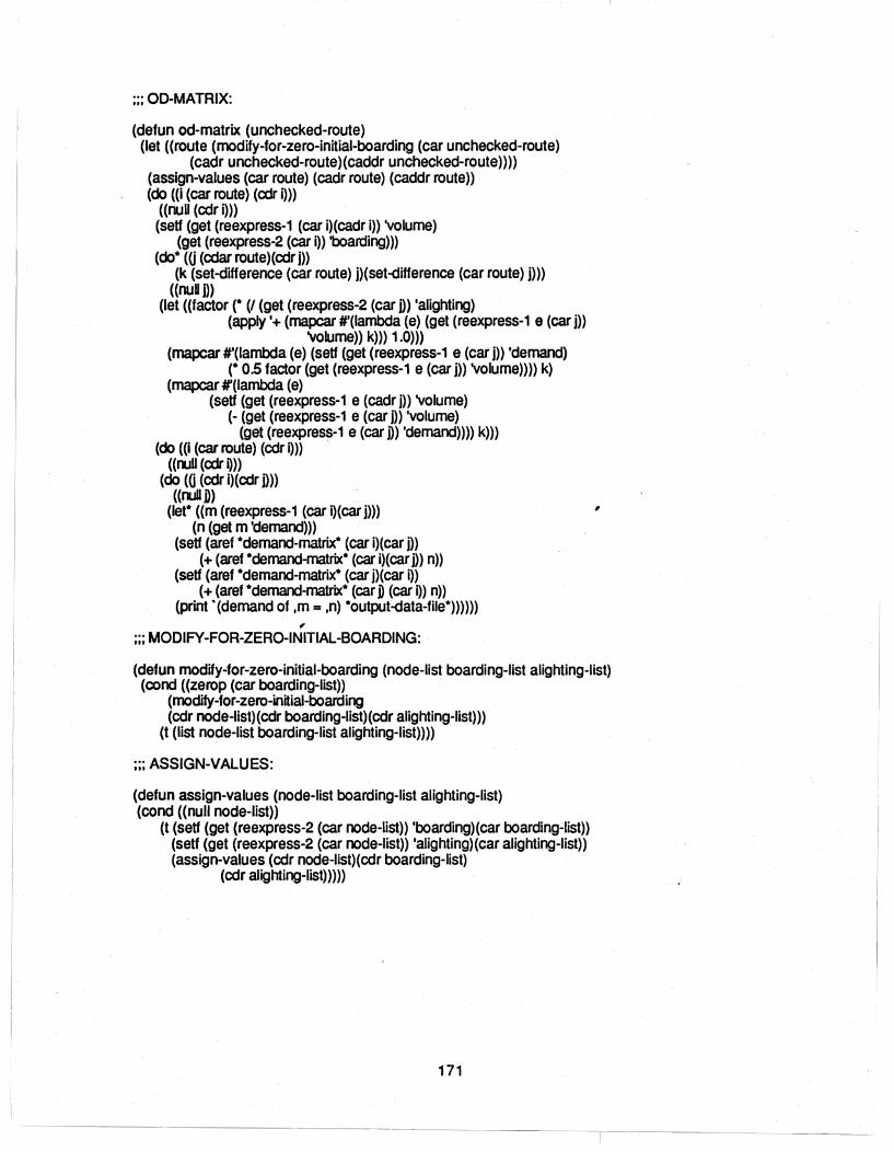
;;; OD-MATRIX:
(detun od-matrix (unchecked-route) (let «route (modity-for-zero-initial-boarding (car unchecked-route)
(cadr unchecked-route)(caddr unchecked-route)))) (assign-values (car route) (cadr route) (caddr route» (do ((i (car route) (cdr i»)
«null (cdr i))) (setf (get (reexpress-1 (car i)(cadr i» 'volume)
(get (reexpress-2 (car i)) 'boarding))) (do* (U (edar route)(cdr j))
(k (set-clifference (car route) j)(set-difference (car route) j))) «nuU j))
(let «tactor (* (/ (get (reexpress-2 (car D) 'alighting) (apply '+ (mapcar #'(Iambda (e) (get (reexpress-1 e (car j))
'volume» k))) 1.0))) (mapcar#'(lambda (e) (setf (get (reexpress-1 e (car j)) 'demand)
(* 0.5 factor (get (reexpress-1 e (car i») 'volume»))) k) (mapcar #,(Iambda (e)
(setf (get (reexpress-1 e (cadr i» 'volume) (- (get (reexpress-1 e (car j») 'volume)
(get (reexpress-1 e (car i» 'demand)))) k))) (do ((i (car route) (cdr Q)
«rull (cdr Q» (do (0 (cdr i)(cdr D»
«J'lJII D) (Iet* «m (reexpress-1 (car i)(car j)))
(n (get m 'demand))) (setf (aret *demand-matrix* (car i)(car j»
(+ (aret *demand-matrix* (car i)(car i» n) (setf (aref *demand-matrix* (car i)(car i»
(+ (aret *demand-matrix* (car D (car i» n» (print' (demand ot ,m = ,n) *output-data-file*))))))
.. ;;; MODIFY-FOR-ZERO-INITIAL-BOARDING:
,
(defun modify-for-zero-initial-boarding (node-list boarding-list alighting-list) (cond «zerop (car boarding-list»
(modify-for -zero-initial-boarding (cdr node-list)(cdr boarding-list)(cdr alighting-list)))
(t (list node-list boarding-list alighting-list»»
;;; ASSIGN-VALUES:
(defun assign-values (node-list boarding-list alighting-list) (cond «null node-list»
(t (setf (get (reexpress-2 (car node-list» 'boarding)(car boarding~list» (setf (get (reexpress-2 (car node-list» 'alighting)(car alighting-list)) (assign-values (cdr node-list)(cdr boarding-list)
(cdr alighting-list»)))
171

C2 Boarding and Alighting Data List
(setf *data-list* «(737271 706968 1 23456789)(239921 52493344 26 5561 1922190)(01 1 2516
293930124265 50 5694» «987654321 68 69 70 71 7273) (9150475837153848 3719 5 4 430) (020231651
51 31 473356602211 11 24» «131211 101 525354555657) (262925241611 127470) (0411 3225411 201616
22» «575655545352 1 1 0 11 12 13)(15 17 15 18 11 11 2221 11 6 0) (0 1 25 10 10 24 2620 28
22» «89888741866321 316171819) (6 1048 74 3911 2322161580)(0431531 294743
12152250» «19181716321 63 8641 878889) (49251491625231511 1211 0) (0 10 14 15 21 24
152032252017) «25 24 23 22 90 10 20 91 43 92 93) (38 23 10 22 27 12 9 5 0 0 0) (0 16 10 9 29 27 15 23 11 2
5» «93924391 20101522232425) (10969142927912180) (0 1 33418209152543» «119118251171161 2 265276282919) (13 19 20 14416191311 44430) (02411
1271416121210121219» . «1929286275262111611725118119)(181111111311182088931 0)(02454
11151713616211710» «1 2103031 3233)(1321 146330)(00211 15 1616» «33 3231301021) (16 15 139200) (023919175» «7312178120123435368373839) (936244 27 21251511 15831 0)(020363030
4938 1931 3222134» «39 38 37 8 36 35 34 2 1 120 78 121 73) (5 15 25 29 31 2253 75 59 ~7 43 27 0) (0 02 11 17
1120 37 26 38 67 93 109» «40414243 44454636819) (563923253230231320) (0243019182332422631» «1983646454443424140) (31 232216108812130) (051013171814122034» «1 234748 49 50 51) (6751 1 1 00)(00266321» «5150494847321)(1 3 4 7 7 2 0 0)(0 01 11 696» «7877767563 15 1034585960 61)(5442231 1 21 1 0)(01 1 1 1 561 11 35» «61 60 59 58 34 10 21 .63 75 76 n 78)(6 4 1 1 3 5 3 1 2 1 1 0)(0 2 2 2 2 2 2 1 1 5 5 5» «26465 66 67) (66 14 21 360) (020222767» «676665 64 2) (37 12 12 19 0) (0 17 10944» «84838281 1 2 62 79 61 8036) (2925172222579730) (061010421 258131536» «368061 796221 81 828384) (75272215352839880) (0 10 12 1721 54 4142025
28» «99 98 97 96 95 94161563 124 125) (734432321 20) (0001 1 238824» «1251246321 16949596979899)(558821 1 1 01 0)(02332223346» «1156259100101 102) (10 169718150) (025682726» « 1 02 101 100 59 62 15 1) (29 25 9 8 9 6 0) (0 12 16 9 11 23 17» «78 69 54 83 66 122 123 128 127 126 52 2 74) (13 5 3 2 2 8 11 5 2 2 2 3 0) (0 2 2 2 3 4 7 7 1 1
31314» «742521261271281231226683546978) (1817201 54342220) (0 1 332614102
23410» «65 129 68 40 130) (5 6 5 2 0) (0 0 3 8 6» «1304068 12965) (6941 0) (00478» «103865910410517106107108) (2417545612230) (026146465629» «108107106171051045986103) (268121611 58160) (024141013971213» «19109110111) (5130) (0 1 36» «11111010919) (3110) (0 104» «19112113114115) (30 1512120) (08102328» «11511411311219) (21191110 0) (08131426»
172
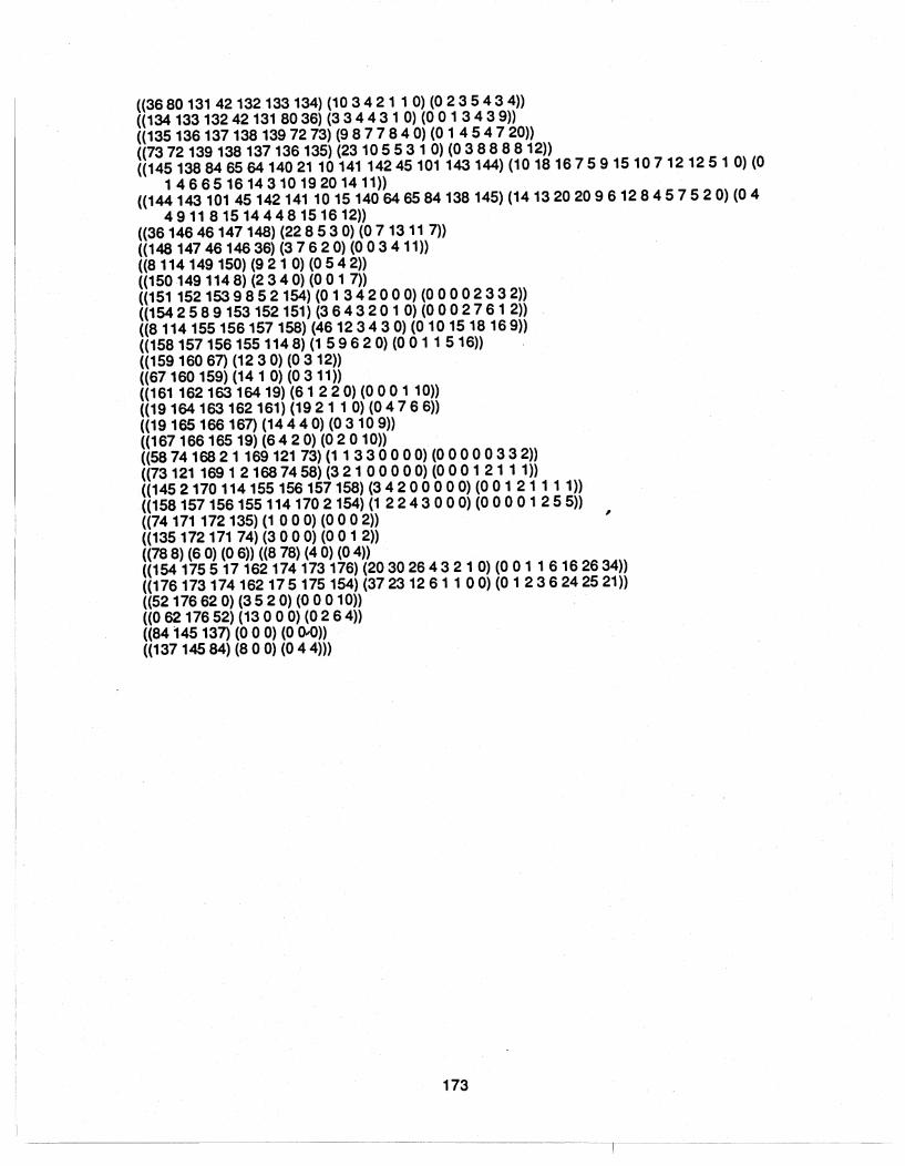
«3680131 42132133134) (103421 1 0) (0235434)) «134 133 13242131 8036) (334431 0) (001 3439)) «135136137138 1397273) (9877840) (0 1 454720)) «7372139138137136135) (23 105531 0) (03888812)) «145138846564140211014114245101143144) (10 18 1675915107121251 0) (0
1 46 65 16 143 10 19 20 14 11)) «144143 101 45142141 101514064 65 84138145) (14 13 20 20 9 6 128457520) (04
4911 81514448151612)) «3614646147148) (228530) (07 13 11 7)) «148 14746146 36) (37620) (003411)) «8114149 150) (921 0) (0542)) «1501491148) (2340) (001 7)) «151 152 153 9 8 5 2154) (0 1 342000) (00002332)) «154 2 5 8 9 153 152 151) (3643201 0) (0002761 2)) «8114155156157158) (46123430) (0 10 1518169)) «1581571561551148){1 5 9 6 2 O){O 011516)) «15916067) (1230) (0312)) «67160 159){14 1 0){0311)) «161 162163 164 19) (61 220) (0001 10)) «19164 163 162161) (19 2 1 1 0) (04766)) «19165 166 167) (14440) (03109)) «167166165 19) (6420) (02010)) «5874168 2 1 169121 73)(1133000 O){O 0000332)) «73121169121687458)(32100000)(00012111)) «1452170114155156157158)(34200000)(00121111)) «1581571561551141702154)(1 2 2 4 3 0 0 O){O 0 0 0 1255)) «74171 172135) (1 000) (0002)) «135172171 74) (3 000) (001 2)) «788) (6 0) (0 6)) «8 78) (4 0) (04))
,
«154175517 162 174 173 176) (2030264321 0) (001 1 6162634)) «176173174162175175154) (37231261 1 00) (0 1 236242521)) «52176620) (3520) (00010)) «06217652) (13000) (0264)) «84145137) (000) (0 ().{))) «137145 84) (8 0 0) (044)))
173

Appendix D Shortest Path Algorithm and K-Shortest Path Algorithm D1 Shortest Path Algorithm
;;; DECLARATIONS:
(defvar *node-Iist*) (defvar *open-Iist*) (defvar *closed-Iist*) (defvar *connectivity-Iist*) (defvar *output-data-file*)
;;; ALL-SHORTEST-PATHS :
(defun all-shortest-paths () (Iet* ((number-of-nodes (length *connectivity-list*»
(*node-list* (generate-list number-of-nodes») (open-output -file) (do* «list-of-nodes *node-Iist* (cdrlist-of-nodes))
(node (car Iist-of-nodes)(car list-of-nodes))) «nulliist-of-nodes) (close *output-data-fiIe*)) (shortest-paths (reexpress-2 node)))))
;;; OPEN-OUTPUT-FILE:
(defun open-output-file 0 (setf*output-data-fiIe*
(open "cm:hd:shih:shortest-paths-output.text" :direction :output :if-exists :append :if-does-not-exist :create)))
;;; SHORTEST-PATHS: ,
(defun shortest-paths (node) (let «*open-Iist* (remove (reexpress-1 node) *node-Iist*))) (mapcar #' (lambda (e)
(setf (get e 'length) 1 e6» *node~list*) (let «i (reexpress-1 node))) (setf (get i 'length) 0.0) (setf *closed-Iist* (list node»)
(generate-all-paths node)))
;;; GENERATE-LIST:
(defun generate-list (number-of-nodes) (do «I 0 (+ i 1»
00» «= i number-of-nodes) D
(setf j (append j (list (reexpress-1 I))))))
;;; GENERATE-ALL-PATHS :
(defun generate-all-paths (node) (Iet* «x (car *closed-Iist*))
. 174
,

(y (get-all-open-edges x)) (z (get (reexpress-1 x) 'length)))
(mapcar #'(lambda (e) (Iet* «m (get e 'length))
(n (+ z (get-time x (reexpress-2 e))))) (cond ((> m n)(setf (get e 'length) n)
(setf (get e 'predecessor) (reexpress-1 x))) (t 0)))) y)
(let «a (next-node-to-close))) (setf *closed-list* (cons (reexpress-2 a) *closed-list*)) (setf *open-list* (remove a *open-list*)) , (cond «null *open-list*) (print-all-paths (reexpress-1 node)))
(t (generate-all-paths node))))))
;;; GET-ALL-OPEN-EDGES :
(defun get-all-open-edges (node) (Iet* «x (cadr (assoc node *connectivity-list*)))
(y (mapcar#' (lambda (e) (reexpress-1 (car e))) x))) (intersection y *open-list*)))
;;; GET-TIME:
(defun get-time (node1 node2) (cadr (assoc node2 (cadr (assoc node1 *connectivity-list*)))))
;;; NEXT-NODE-TO-CLOSE :
(defun next-node-to-close () (caar (sort (mapcar #' (lambda (e)
(list e (get e 'length))) *open-list*) #' < :key 'cadr)))
;;; PRINT-ALl-PATHS: ,
(defun print-all-paths (node) (setf x (remove node *node-list*)) (do* «i x (cdr i))
o (car i)(car~)) «nuO i))
(coro ((> (reexpress-2 j) (reexpress-2 node)) (list-path node j j (get j 'Iength)(list (reexpress-2 j))))
(t 0))))
;;; LIST-PATH:
(defun list-path (node1 node2 node3 path-length answer-list) (let «x (get node3 'predecessor))
(a (reexpress-2 node1)) (b (reexpress-2 node2)) (c (/ (round (* 10.0 path-length)) 10.0)) (d (cons (reexpress-2 node1) answer-list)))
(cond «equal x node1) (format *output-data-file* "_% (-a -a -a -a)" abc d))
175
,
-- .~ ----- -

(t (list-path node1 node2 x path-length (cons (reexpress-2 x) answer-list))))))
;;; REEXPRESS-1 :
(defun reexpress-1 (node) (read (make-string-input-stream
(format nil "-a-a" 'node- node))))
;;; REEXPRESS-2 :
(defun reexpress-2 (node) (read (make-string-input-stream node 5»))
;;; Require ·CONNECTIVITY-LiSr as input
,
176
,

02 k-Shortest Path Algorithm
;;; DECLARATIONS:
(defvar *number-of-nodes*) (defvar *number-of-paths*) (defvar *list-of-nodes*) (defvar *node-list*) (defvar *open-list*) (defvar * connectivity-list*) (defvar *output-data-file*) (defvar *reduced-list*) (defvar *selected-list*)
;;; ALL-K-SHORTEST-PATHS :
(defun all-k-shortest-paths (k) (Iet* «*number-of-nodes* (length *connectivity-list*))
(*number-of-paths* k) (*list-of-nQdes* (generate-list1)))
(open-output-file) (do* «x *Iist-of-nodes* (cdr x))
(node (car x)(car x))) «null x) (close *output-data-file*))
(k-shortest-paths (reexpress-3 node)))))
;;; OPEN-OUTPUT-FILE :
(detun open-output-file () (setf *output-data-file*
(open ·cm:hd:shih :k-shortest-paths.text" :direction :output
;;; START:
:if-exists :append :if-does-ROt-exist :create)))
(defun start () (open-output-file) (do* ((i *selected-list* (cdr i))
a (car Q(car Q) (k (car D(car j)) (m (cadr D(cadr j))) «null i) (close *output-data-file*))
(setf *reduced-list* m) (k-shortest-paths k)))
;:; K-SHORTEST-PATHS:
(defun k-shortest-paths (node) (setf *number-of-paths* 6) (setf *number-of-nodes* 177) (setf *list-of-nodes* (generate-list1» (Iet* «*open-list* (generate-list2))
177
,

(*node-list* *open-list*)) (setf *list-of-nodes* (remove (reexpress-1 node) *list-of-nodes*)) (mapcar #' (lambda (e)
(setf *node-list* (remove e *node-list*)))
(get (reexpress-1 node) 'node-names)) (mapcar #' (lambda (e)
(setf (get e 'length) 90)) *open-list*) (let «x (reexpress-2 node 1))) (setf (get x 'predecessor) x) (setf (get x 'length) 0.0) (generate-all-k-paths node))))
;;; GENERATE-uSn:
(defun generate-list1 () (do «i 0 (+ i 1))
00)) «= i *number-of-nodes*) D
(setf j (append j (list (reexpress-1 Q)))))
;;; GENERATE-UST2 :
(detun generate-list2 () (do «i 0 (+ i 1))
00)) «= i *number-of-nodes*) D
(let «x (make-node-names i))) (setf j (append jx)))))
;;; MAKE-NODE-NAMES :
(detun make-node-names (node) (do «i 1 (+ i 1)) ,
00)) «= i (+ *number-ot-paths* 1)) (let «x (reexpress-1 node))) (setf (get x 'node1) node) (setf (get x 'node-names) j) j))
(let «y (reexpress-2 node i))) (setf (get y 'node1) node) (setf (get y 'node2) Q (setf j (append j (list y))))))
;;; GENERATE-ALL-K-PATHS :
(defun generate-all-k-paths (node) (Iet* «i (next-node-to-close))
(j (get i 'length)) (k (get i 'node1)) (m (get-neighboring-nodes k)) (n (open-adjacent-nodes m)))
(mapcar #' (lambda (e) (adjust -costs-predece ssors e (+ j (get-time k (get (car e) 'node1))) i))
178
,

n) (setf *open-Ust* (remove i *open-Iist*)) (cond «null *open-Iist*)
(assign-all-k-paths (reexpress-2 node 1)) (list-two-paths node))
(t (generate-all-k-paths node)))))
;;; NEXT-NODE-TO-CLOSE :
(defun next-node-to-close 0 (caar (sort (mapcar #' (lambda (e)
(list e (get e 'length))) *open-Iist*) #' < :key 'cadr)))
;;; GET-NEIGHBORING-NODES :
(defun get-neighboring-nodes (node) (let ({x (cadr (assoc node *connectivity-Iist*)))) (mapcar#' (lambda (e)
(reexpress-1 (car e))) x)))
;;; OPEN-ADJACENT-NODES :
(defun open-adjacent-nodes (list-of-nodes) (remove-if #'nuU (mapcar #' (lambda (e)
(intersection (get e 'node-names) *open-Iist*))
list-of-nodes )))
;;; ADJUST-COSTS-PREDECESSORS :
(defun adjust-costs-predecessors (list-of-nodes c p) (cond ({> (get (car (last Iist-of-nodes)) 'length))
(let· «x (remove-it-not #' (lamtxJa (e) (> (get e 'length) c))
Iist-of-nodes)) (y (reverse x)) (z (car x)))
(switch-costs-predecessors y) (setf (get z 'length) c) (setf (get z 'predecessor) p)))
(t 0)))
;;; SWITCH-COSTS-PREDECESSORS :
(defun switch-costs-predecessors (list-of-nodes) (cond «null (cdr Iist-of-nodes)) ())
(t (let «x (get (cadr Iist-of-nodes) 'length)) (y (get (cadr Iist-of-nodes) 'predecessor)))
(setf (get (car Iist-of-nodes) 'length) x) (setf (get (car Iist-of-nodes) 'predecessor) y))
(switch-costs-predecessors (cdr Iist-of-nodes)))))
;;;GET-TIME:
179
,
-I ----- -- -

(defun get-time (node1 node2) (cadr (assoc node2 (cadr (assoc'node1 "connectivity-list")))))
;;; ASSIGN-ALL-K-PATHS :
(defun assign-all-k-paths (node) . (do" «i "node-list" (cdr Q) a (car i)(car Q»
«ruB Q) (assign-k-path node j j (get j 'Iength)(list (get j 'node1»))))
;;; ASSIGN-K-PATH :
(defun assign-k-path (n1 n2 n3 path-length path-list) (let «x (get n3 'predecessor))) (cond «= path-length 90)
(setf (get (reexpress-1 (get n2 'node1» 'path-condition) 'no-path)) ,
«equal x n1) (setf (get n2 'path-Iength)(/ (round (" 10.0 path-length)) 1 0.0» (setf (get n2 'path-list) (cons (get n1 'node1) path-list))) (t(assign-k-path n1 n2 x path-length
(cons (get x 'node1) path-list))))))
;;; LlST-TWO-PATHS :
(defun list-two-paths (node) (do" ((i "Ust-of-nodes· (cdr i))
a (car i)(car Q» «ruB Q) . (cond «not (member (reexpress-3 j) "reduced-list·)))
(t (determine-two-pa~s node j))))).
;;; DETERMINE-TWO-PATHS :
(defun detennine-two-paths (n1 n2) (let· «x (get n2 'path-condition»
(y (get n2 'node-names)) (shortest-path (car y)))
(cond «equal x 'no-path)(print (list n1 (get n2 'node1)()))) (t(find-two-paths
n1 n2 (cdry) (get shortest-path 'path-length) (get shortest-path 'path-list»»»
;;; FIND-TWO-PATHS:
(defun find-two-paths (n1 n2 list-of-paths a b) (let· «x (car list-of-paths»
(y (get x 'path-length» (z (get x 'path-list)))
(cond «nuillist-of-paths) (print (list n1 (get n2 'node1 )(list a b)())
180
;

·output-data-file*)) «and «= y (* 1.50 a))
(not (cyclical? z)) (different-links? z b))
(print (list n1 (get n2 'node1)(list a b) (list y z)) *output -data-file *))
(t (find-two-paths n1 n2 (cdr Iist-ot-paths) a b)))))
;;; CYCLICAL? :
(defun cyclical? (list-ot-nodes) (cond «= (length list-ot-nodes)
(length (remove-duplicates list-ot-nodes))) ()) (t t)))
;;; DIFFERENT-LINKS? :
(detun different-links? (next-shortest~path shortest-path) (cond «<= (common-links next-shortest-path shortest-path 0)
(* 0.5 (- (length next-shortest-path) 1))). t) . (t 0)))
;;; COMMON-LINKS:
(defun common-links (list1 Iist2 number-of-common-Iinks) (cond «null (cdr Iist1)) number-of-common-links)
«and (member (car 6st1) list2) (member (car list1) Iist2))
(common-links (cdr Iist1) Iist2 (+ number-ot-common-links 1))) (t (common-links (cdr Iist1) Iist2 number-ot-common-links))))
;;; REEXPRESS-1 :
(detun reexpress-1 (node), (read (make-string-input-stream
(format nil "-a-a" 'node- node))))
;;; REEXPRESS-2 :
(detun reexpress-2 (node1 node2) (read (make-string-input-stream
(format nil "-a-a-a-a" 'node- node1 '- node2))))
;;; REEXPRESS-3 :
(defun reexpress-3 (node) (read (make-string-input-stream node 5)))
;;; ·SELECTED-LiSr Example:
(setf ·selected-list· '«34 (35 33 32)) (8 (12 9))(14 (1912))(123 (122 128))(78 (75 79)) (54 (53 55))(72 (71 73))(82 (81 89))(103 (87124))))
;;; Require ·CONNECTIVITY -L1sr as input.
181 .

REFERENCES
Abkowitz, M., Josef, R., Tozzi, J., and Driscoll (1987), "Operational Feasibility of Timed Transfer in
Transit Systems," Journal of Transportation Engineering, Vol. 113, No.2, P 168-177,
ASCE.
American Public Transit Association, (1991), Transit Fact Book, Washington, DC, 1991.
Baaj, M. H. (1990), The TransH Network Design Problem: An AI-Based Approach, Ph.D. thesis,
Department of Civil Engineering, University of Texas, Austin, Texas.
Baaj, M. H. and Mahmassani, H. S. (1990), "TRUST: A Lisp Program for the Analysis of Transit
Route Configuration," Transportation Research Record 1283, Transportation Research
Board, Washington, D.C., p 125-135.
Baaj, M. H. and Mahmassani, H. S. (1991), "An AI-Based Approach for Transit Route System
Planning and Design," Journal of Advanced Transportation Vol. 25, No.2, P 187-210.
Baaj, M. H. and Mahmassani, H. S. (1992), "Artificial Intelligence-Based System Representation
and Search Procedures for Transit Route Network DeSign," Transportation Research
Record 1358, Transportation Research Board, Washington, D.C., p 67-70.
Bakker, J. J., Calkin, J., and Sylvester, S. (1988), "Multi-Centered Timed-Transfer System for
Capital Metro, Austin, Texas," Transportation Research Record 1202, Transportation
Research Board, Washington, D.C., p 22-28.
Bly, P. H. and Oldfield, R. H. (1986), "Competition Between Minibuses and Regular Bus Service,"
"Journal of Transport Economics andPoUcy 20 (1), p 47-68. , Bowman, L. A. and Turnquist, M. A. (1981), "Service Frequency, Schedule Reliability and
Passenger Wait Times at Transit Stops," Transportation Research, Vol. 15A, No.6, P
465-471.
Ceder, R. B. and Wilson, N. H. (1986), "Bus Network Design," Transportation Research, Vol. 208,
No.4, P 331-344.
Cervero, R. (1986), Suburban Gridlock, Rutgers, Center for Urban Policy Research, The State
University of New Jersey, New Brunswick, N.J ..
Chang, S. K. (1990), AnalytiC Optimization of Bus Systems in Heterogeneous Environment,
Ph.D. thesis, Department of Civil Engineering, University of Maryland, College Park,
Maryland.
Chang, S. K. and Schonfeld, P. M. (1991), "Integration of Fixed- and Flexible-Route Bus
System," Transportation Research Record 1308, Transportation Research Board,
Washington, D.C., p 51-57.
182
Daganzo, C. F., Hendrickson, C. T., and Wilson, N. H. M. (1977), "An Approximate Analytic Model
of Many-to-One Demand Responsive Transportation Systems," Proc. 7th Int. Symp. on
Transportation and Traffic Theory, Kyoto, Japan, p 743-772.
D.ial R. B. (1967), "Transit Pathfinder Algorithm," Highway Research Record 205, p 67 - 85.
Dijkstra, E. W. (1959), "A Note on Two Problems in Connection with Graphs," Numerische
Mathematik, Vol. 1, p 269-271.
Dubois, D., Bell, G., and Llibre, M. (1979), "A Set of Methods in Transportation Network SyntheSiS
and Analysis," Journal of Operations Research Society 30, p 797-808.
Florian M. and Speiss H. (1983), "On Two Mode Choice/Assignment Models," Transportation
Science 17, p 32-47.
Furth, P. G. and Wilson, N. H. M. (1981), "Setting Frequencies on Bus Routes: Theory and
Practice," Transportation Research Record 818, Transportation Research Board,
Washington, D.C., p 1-7.
Glaister, S. (1985), "Competition on an Urban Bus Route," Journal of Transport Economics and
fQ.Jb.19 (1), p 65-81.
Glaister, S. (1986), "Bus deregulation, Competition and Vehicle Size," Journal of Transport
Economics and Policy 20 (2), P 217-244. '
Gwilliam, K. M., Nash C. A., and Mackie P. J. (1985), "Deregulating the Bus Industry in Britain-The
Case Against," Transport Rey, 5 (2), p 105-132.
Han A. F. and Wilson N. H. M. (1982), "The Allocation of Buses in Heavily Utilized Networks with
Overlapping Routes," Transportation Research, Vol. 16B, No.3, p221-232. , Hasselstrom, D. (1981), Public Transportation Planning - A Mathematical Programming Approach,
Ph.D. thesis, Department of Business Administration, University of Gothenburg,
Sweden.
Herman, B. and Ardekani, S. (1984), "Characterizing Traffic Conditions in Urban Areas,"
Transportation Science Vol. 18, No.2, p101-140.
Israeli, Y. and Ceder, A. (1991), "Transit Network Design," Presented at the 70th Annual Meeting
of Transportation Research Board, Washington, D.C ..
Jansson, J. O. (1980), "A Simple Bus Line Model for Optimization of Service Frequency and Bus
Size," Journal of Transport Economics and Policy 14 (1), p 53-80.
Lampkin, W. and Saalmans, P. D. (1967). "The Design of Routes, Service Frequencies and
Schedules for a Municipal Bus Undertaking: A Case Study,". Operation Research
Quarterly 18, p 375-397.
183

Larson. R. C. and Odoni. A. R. (1981). Urban Operations Research. Prentice-Hall Inc .• Englewood
Cliffs. New Jersey.
LeBlanc. l. J. (1988). "Transit System Network Design." Transportation Research B. Vol. 22B.
No.5. P 383-390.
Uu. Y. H. (1994). An Approach for the Characterization and ClassUication of Bus Transit Network
Structure. Master Thesis. Department of Civil Engineering. University of Texas. Austin.
Texas.
Mandl, C. E. (1979). "Evaluation and Optimization of Urban Public Transportation Networks."
Presented at the 3rd European Congress on Operations Research. Amsterdam.
Netherlands.
Mohring. H. (1972). "Optimization and Scale Economies in Urban Bus Transportation." American
Economic Review.
Mohring. H. (1983). "Minibuses in Urban Transportation." Journal of Urban Economics 14, p293-
317.
NCHRP Synthesis of Highway Practice 69 (1980). Bus Route and Schedule Plannjog Guidelines.
Transportation Research Board. National Research Council. Washington. D.C ..
Newman. D. A .• Bebendorf, M .• and McNally, J. (1983). Tjmed-Transler: An Evaluation of its
Structure. Performance and Cost, Urban Mass Transportation Administration. U.S. DOT.
Washington, D.C ..
Newell. C. E. (1979). "Some Issues Related to the Optimal Design of Bus Routes." Transportation
SCience 13. p 20-~5
Oldfield. R. H. and Bly. P. H. (1988). "An Analytic Investigation of Optimal Bus Size."
Transportation Research B, Vol. 22B. No.5. P 319-337.
Osuna. E. E. and Newell. G. F. (1972). "Control Strategies for an Idealized Public Transportation
System." Transportation Science 6. p. 57-72.
Rapp M. H .• Mattenberger P .• Piguet S .• and Robert-Grandpierre A. (1976) "Interactive Graphic
System for Transit Route Optimization."Transportation Research Record 619. p 27-33.
Rea. J. C. (1971). "Designing Urban Transit Systems: An Approach to the Rout-Technology
Selection Problem," PB 204881. University of Washington. Seattle. WA.
Schneider, J. and Smith. S. (1981). "Redesigning Urban Transit Systems: A Transit-Center
Based Approach. II Transportation Research Record 798, Transportation Research Board.
Washington. D.C .• p 56-65.
Shier D. R. (1979). "On Algorithms for Finding the K Shortest Paths in a Network." Networks. Vol.
9, p 195 - 214.
184

Shih, M. C. and Mahmassani, H. S. (1994), "A Vehicle Sizing Model for Bus Transit Systems,"
presented at the 73th Annual Meeting of the Transportation Research Board,
Washington, D.C ..
Silman, L. A., Barzily, Z., and Passy, U. (1974), "Planning the Route System for Urban Buses,"
Computers and Operations Research 1, p 201-211.
Simon, J. and Furth, P. G. (1985), "Generating a Bus Route 0-0 Matrix from On-Off Data," Journal
of Transportatjon Engineering, Vol. III, No.6, P 583-593.
Speiss, H. and Florian, M. (1989), "Optimal Strategies: A New Assignment Model for Transit
Networks," Transportation Research B, Vol. 23, No.2, P 83-102.
Taylor-Harris, A. and Stone, T. J. (1980) "Transit Center: A Means of Improving Transit Services,"
Transportation Research Record 760, p 39-42.
Tri-County M.T.D. (1982), "Planning, Implementation and Evaluation of aTimed-Transfer System
in Portland, Oregon's Suburban Westside," Tri-County MetropOlitan Transportation
District of Oregon, Portland, Oregon.
Tsygalnitzky, S. (1979), Simplified Methods of Transportatjon Planning, Master ThesiS,
Massachusetts Institute of Technology, Cambridge, Massachusetts. ,
Van Nes, R., Hamerslag, R., and Immer, B. H. (1988), "The Design of Public Transport Networks,"
Transportation Research Record 1202, Transportation Research Board, Washington,
D.C., p 74-83.
Walters, A. A. (1979), "The Benefit of Minibuses," Journal of Transport Economics and policy 14
(3), P 320-334. ,
Walters, A. A. (1982), "Externalities in Urban Buses," Journal of Urban Economics 11, p 60-72.
Wilson, N. H. M.(1982), "Bus Service Planning; Current Practice and New Approaches," Working
Paper, Massachusetts Institute of Technology, Cambridge, Massachusetts.
Wilson, N. H. M. and Gonzalez S. l. (1982), "Methods for Service Design," Transportation
Research Record 862, Transportation Research Board, Washington, D.C., p 74-83.
185