A Democratic Measure of Household Income Growth: Theory and Application to the United Kingdom

Andrew Aitken1,2 and Martin Weale3,4

1,3Economic Statistics Centre of Excellence

2National Institute of Economic and Social Research

4Centre for Macroeconomics and King’s College, London

ESCoE Discussion Paper 2018-02

February 2018

ISSN 2515-4664

About the Economic Statistics Centre of Excellence (ESCoE)

The Economic Statistics Centre of Excellence provides research that addresses the

challenges of measuring the modern economy, as recommended by Professor Sir

Charles Bean in his Independent Review of UK Economics Statistics. ESCoE is an

independent research centre sponsored by the Office for National Statistics (ONS).

Key areas of investigation include: National Accounts and Beyond GDP, Productivity

and the Modern economy, Regional and Labour Market statistics.

ESCoE is made up of a consortium of leading institutions led by the National Institute

of Economic and Social Research (NIESR) with King’s College London, innovation

foundation Nesta, University of Cambridge, Warwick Business School (University of

Warwick) and Strathclyde Business School.

ESCoE Discussion Papers describe research in progress by the author(s) and are

published to elicit comments and to further debate. Any views expressed are solely

those of the author(s) and so cannot be taken to represent those of the ESCoE, its

partner institutions or the ONS.

For more information on ESCoE see www.escoe.ac.uk.

Contact Details Economic Statistics Centre of Excellence National Institute of Economic and Social Research 2 Dean Trench St London SW1P 3HE United Kingdom T: +44 (0)20 7222 7665 E: escoeinfo@niesr.ac.uk

A Democratic Measure of Household Income Growth: Theory and Application to the United Kingdom

Andrew Aitken1,2 and Martin Weale3,4,5

1,3Economic Statistics Centre of Excellence, 2National Institute of Economic and

Social Research, 4Centre for Macroeconomics and King’s College, London

Abstract This paper develops a price and quantity system of indicators structured round

Atkinson's concept of inequality aversion. A democratic indicator of income growth,

weighting each household's growth experience equally, is shown to result when

Prais' democratic price index is used to deflate the geometric mean of equivalised

household income. A welfare interpretation of the democratic indicator of income

growth is provided and it is shown that, with heterogeneous but homothetic

preferences, the deflator can serve as a common scaling social cost of living index

when applied to income as well as to consumption. Application to United Kingdom

household data suggests that, over the interval 2005/6-2015/6 democratic real

equivalised household income grew by 0.20 per cent per annum while the plutocratic

equivalent grew by 0.52 per cent per annum.

Key words: Real Income, Inequality Aversion, Welfare Indicator, Cost of Living

JEL classification: I31, D12, E21

Contact Details Martin Weale Economic Statistics Centre of Excellence National Institute of Economic and Social Research 2 Dean Trench St London SW1P 3HE Email: a.aitken@niesr.ac.uk, martin.weale@outlook.com This ESCoE paper was first published in February 2018.

© Andrew Aitken and Martin Weale

5 We are very grateful to ESCoE for financial support, to Tanya Flower of the Office for National

Statistics for providing the democratic price index used in this paper, and to Tom Crossley and Nick Oulton for very helpful discussions.

1 Introduction

In this paper we develop aggregate price and quantity indices which reflect inequality

aversion of the type described by Atkinson (1970). We show in particular that, when

a nominal aggregate is constructed as the geometric mean of household income and

that aggregate is deflated using an appropriate democratic price index which gives equal

weight to the expenditure patterns of each household (Prais 1958), the resulting quantity

variable is an index whose growth is the arithmetic average of each household’s growth in

real income. Following Prais (1958) it can therefore be described as a democratic measure

of household real income growth with the property that it treats each household’s growth

experience equally. Newbery (1995) used a similar approach to explore the welfare effects

of price changes in Hungary and the United Kingdom but otherwise, as far as we know,

the relationship between Atkinson’s approach and price and quantity indicators has not

been explored.

The need for indicators which, unlike GDP are sensitive to the distribution of resources

is well documented. The Stiglitz Commission (Stiglitz, Sen, and Fitoussi 2009) observed

that “if inequality increases enough relative to the increase in the average of per capita

GDP, then most people can be worse off even though average income is increasing”. Jor-

genson and Slesnick (2014) following Jorgenson (1990) suggest addressing this issue by

basing a welfare measure on consumption rather than income or output; their proposal is

to use an econometrically estimated demand system to provide the structure needed to

produce a cardinal measure of utility, and they present a welfare indicator for the United

States on that basis. In this econometric framework utility is calculated per household,

with each household’s circumstances reflected in an econometrically-estimated equiva-

lence scale which takes account not only of household composition but also of other

factors such as age and location. In a similar vein Oulton (2008) explored a Konus price

index for the United Kingdom, estimating the cost of obtaining the consumption which

would deliver a fixed level of utility for a representative household.

A related literature has evolved from the work by Pollak (1981) who explored the de-

velopment of a social cost of living index. His approach was to calculate the increase

in expenditure needed to deliver a particular level of welfare, on the assumption that

resources were allocated to optimise the relevant social welfare function. Crossley and

2

Pendakur (2010) have extended the concept to a constant-scaling social cost of liv-

ing index (CS-SCOLI); they show how, given knowledge of the actual distribution of

consumption, each household’s welfare function and the means by which these are ag-

gregated into the relevant social welfare function, it is possible to define the change in

the cost of living associated with a given change in prices as the proportionate increase

in each household’s expenditure required to restore the social welfare function to its

previous value. Thus, in contrast to Pollak (1981), they work with reference to the

distribution of resources as it actually is. Of course constant scaling may leave some

households better off and others worse off if their consumption patterns differ, but for

policy purposes such as the adjustment of state benefits it is probably the most relevant

approach. Nevertheless, their work, like Jorgenson and Slesnick (2014), requires econo-

metric estimation of a demand system. They make no attempt to develop a cardinal

measure of social welfare or any other type of quantity indicator.

Jorgenson and Schreyer (2017) recognise, however, that approaches of this type are

unlikely to appeal strongly to statistical offices. They therefore suggest a simplified wel-

fare indicator compiled by adjusting household consumption for household size using a

standard equivalence scale such as the square root scale (Organisation for Economic Co-

operation and Development 2011). After scaling and deflation Jorgenson and Schreyer

(2017) suggest combining the household figures using Atkinson’s inequality aversion ap-

proach1 with the inequality aversion parameter set to a value designed, for the United

States at least, to approximate to the median household. They note that there is an

issue with deflation because different households buy different things, and suggest split-

ting households into quintiles defined over equivalent consumption, with deflators re-

flecting the spending patterns of those quintiles. They do not, however, explore the

price/quantity/value inter-relationship arising from their measures.

This measure is structured round consumption rather than income. There are two rea-

sons for this. Slesnick (1998) observes that households with temporarily low incomes

will maintain their consumption, while those with temporarily high incomes will be high

savers; consumption may therefore be a better indicator of life-time income and thus

life-time resources than is current income. Secondly, a focus on consumption makes it

straightforward to draw on the wide body of consumer theory providing an underpin-

1They also present an alternative adjustment for inequality developed by Jorgenson and Slesnick(1983) but which is not used as widely as Atkinson’s approach.

3

ning for the approaches suggested by Crossley and Pendakur (2010) and Jorgenson and

Slesnick (2014). On the other hand there have been a number of attempts to give a

welfare interpretation to income rather than consumption. At an aggregate level Weitz-

man (1976) suggested that net national income, measured in consumption terms, was,

subject to a linear approximation, equal to sustainable consumption and thus could be

seen as a welfare indicator. Sefton and Weale (2006) developed Weitzman’s analysis,

first on an individual and then on an aggregate basis. They showed that, in an economy

in which capital was being accumulated or decumulated, it was not possible to equate

income and sustainable consumption but that net saving multiplied by the marginal

utility of money was nevertheless equal to the increase in lifetime utility in which it gave

rise.

Here we build on that result to provide an interpretation of growth in real income for

each household in terms of an associated increase in life-time utility. We show that,

with a democratic measure of real income growth, each household’s increase in life-time

utility is measured with respect to its own marginal utility of consumption while the

conventional measure is defined with respect to average marginal utility of consumption.

These results require that households have homothetic but not necessarily homogenous

preferences. While it is clear that household preferences cannot be represented by a single

homothetic preference function, Redding and Weinstein (2016) argue that movements in

household consumption patterns are better explained by preference shifts than by more

traditional aggregate preference functions. Further, their analysis of scanner data from

the United States of America suggests that these preference shifts are entirely compatible

with the requirements of homotheticity.

Finally, again given the assumption of homothetic but heterogeneous preferences possi-

bly affected by preference shocks, we show that the democratic price index and quantity

growth indicator emerge if each household’s utility is logarithmic in its deflated consump-

tion aggregate. We demonstrate that, in these circumstances, the democratic Divisia

price index is a CS-SCOLI. We show further that, to a first order approximation, wel-

fare accruing can coherently be represented as a utility function in terms of income;

the democratic Divisia price index again emerges as a CS-SCOLI and the associated

democratic measure of income growth represents the rate of growth of an index of social

welfare. Thus, the same system of price and quantity indices is derived whether one

4

works heuristically from Atkinson inequality aversion with an aversion parameter of one

or from a logarithmic household utility function. Our theoretical analysis is set out en-

tirely in terms of continuous time. Application requires chain-linking of the type which

is now widespread.

This paper proceeds as follows. Section 2 describes our notation. Section 3 explains

the connection between democratic price and quantity indices and Atkinson’s concept of

inequality aversion. Section 4 provides a welfare interpretation of democratic income and

section 5 explains the relationship with constant scaling cost of living indices. Section 6

presents results for the UK and section 7 concludes.

2 Notation

We use lower case letters to refer to individual households and upper case letters to refer

to aggregates. πt is the vector of prices in the economy at time t, with the jth element,

πjt indicating the price of good j and cit is the vector of equivalised consumption of

household i with cijt the consumption of good j. yit is its equivalised money income

and xit is its equivalised money spending on consumption goods. ui(cit) is the utility

derived from equivalised consumption by household i, and zi(πt, xit) is indirect utility

from equivalised consumption xit; ωit is the vector of expenditure shares measured as

a fraction of total consumption, and ωijt is the share of expenditure by household i on

good j. pit is a consumption price index for household i and qit = yit/pit is its equivalised

real income. r∗t is the money rate of interest and rit is the real interest rate faced by

household i; different households have different real interest rates because they have

different consumption patterns. ρ is the degree of inequality aversion, and σ is the

intertemporal elasticity of substitution. Yt(ρ), Pt(ρ) and Qt(ρ) are aggregate variables

representing income, prices and quantities defined precisely as they are introduced. Our

analysis is in continuous time; we use the symbol ∆ to indicate the difference between

one continuous time path and another.

In this paper we do not discuss equivalisation but simply assume that all income and

consumption variables have been adjusted for household composition using a standard

equivalence scale. References to household income and consumption are thus shorthand

for references to equivalised income and consumption.

5

3 Atkinson Inequality Indices and a Democratic Mea-

sure of Income Growth

3.1 Derivation of Quantity Indices

Atkinson (1970) developed the concept of inequality aversion. For a population of N

households, with household i having an income of yit in period t. Atkinson’s inequality-

adjusted measure of average income is defined as

Yt(ρ) =1

N(N∑i=1

y1−ρit )1

1−ρ with ρ ≥ 0 and ρ 6= 1 (1)

Yt(1) = N

√√√√ N∏i=1

yit ρ = 1

Each household’s income is the product of its price index pit and its real income qit;

yit = pitqit.

Suppose we now express Yt(ρ) as the product of aggregate price and quantity measures

Yt(ρ) = Pt(ρ)Qt(ρ) =1

N(N∑i=1

p1−ρit q1−ρit )1

1−ρ with ρ ≥ 0 and ρ 6= 1 (2)

We now take logarithms and differentiate with respect to time, with the expression valid

even if ρ = 1

Pt(ρ)

Pt(ρ)+Qt(ρ)

Qt(ρ)=

∑Ni=1

(pitpitp1−ρit q1−ρit + qit

qitp1−ρit q1−ρit

)∑N

i=1 p1−ρit q1−ρit

(3)

=

∑Ni=1

(pitpit

+ qitqit

)y1−ρit /Y 1−ρ

t (ρ)

N

This makes it natural to define the growth in the price and quantity indices as

Pt(ρ)

Pt(ρ)=

∑Ni=1

pitpity1−ρit /Y 1−ρ

t (ρ)

N(4)

andQt(ρ)

Qt(ρ)=

∑Ni=1

qitqity1−ρit /Y 1−ρ

t (ρ)

N(5)

6

We can now see very clearly that, in the special case where there is no inequality aversion

(ρ = 0) the growth rates of the aggregate price and quantity indices are the growth

rates experienced by the individual households weighted together by their shares in

total money income. On the other hand, if ρ = 1, then the price and quantity indices

are simply the arithmetic averages of the growth experiences of individual households.

Each household has an equal influence on the growth of the aggregates, and in that

sense Qt(1)/Qt(1) is, following Prais (1958) who described the price index with ρ =

1 as democratic, a democratic measure of income growth. In contrast Qt(0)/Qt(0)

because it weights the household experiences by their income levels, can be described as

a plutocratic measure.

There remains the question of how to calculate either the price or the quantity index for

each household. We assume that it is easier to measure prices than volumes, and that

changes in quantity indices have to be derived from changes in values and changes in

price indices, both individually and at an aggregate level. To proceed it is necessary to

consider the “real” price of good j to household i, πjt/pit. The price index, pit is defined

by the condition that, when the household has optimised its consumption, in the light

of the prevailing prices, the cost of the consumption basket in real prices is constant as

nominal prices change:∑j

cijtd (πjt/pit)

dt=∑j

cijtpitπjt − πjtpit

p2it= 0 (6)

or ∑j

cijtπjtpit

=pitp2it

∑j

cijtπjt (7)

givingpitpit

=

∑j cijtπjt∑j cijtπjt

=∑j

ωijtπjtπjt

(8)

This, of course, is the equation for the growth of the Divisia price index specific to

household i.

Combining this with equation 4, we can write

Pt(ρ)

Pt(ρ)=

∑Ni=1

∑j ωijt

πjtπjty1−ρit /Y 1−ρ

t (ρ)

N(9)

=

∑jπjtπjt

∑Ni=1 ωijty

1−ρit /Y 1−ρ

t (ρ)

N

7

The growth of the aggregate price index is itself the weighted sum of the growth rates of

the individual prices. The weights depend on the consumption patterns of the individual

households themselves weighted together by each household’s inequality-adjusted income

relative to inequality adjusted average income. In the special case where ρ = 1 we have

Pt(1)

Pt(1)=

∑jπjtπjt

∑Ni=1 ωijt

N. (10)

In this case, then, the weights applied to the growth of each price are the arithmetic

averages of each household’s expenditure shares. This is exactly the Divisia form of the

democratic price index suggested by Prais (1958). In other cases, however, it should be

noted that the weights depend on income rather than on consumption.

Growth in the aggregate quantity index is then defined as

Qt(ρ)

Qt(ρ)=Yt (ρ)

Yt(ρ)−∑

jπjπj

∑Ni=1 ωijty

1−ρit /Y 1−ρ

t (ρ)

N(11)

Integrating up and using subscripts to indicate time, we can write

logQt(ρ)

Qt0(ρ)= log

Yt(ρ)

Yt0(ρ)−∫ t

t0

∑jπjτπjτ

∑Ni=1 ωijτy

1−ρiτ /Y 1−ρ

τ (ρ)

Ndτ (12)

In practice of course it is not possible to construct the Divisia price index required. But

we could calculate Pt(ρ) as a chain-linked price index, making it possible to define

Qt(ρ)

Qt0(ρ)=

Yt(ρ)

Yt0(ρ)

Pt0(ρ)

Pt(ρ)(13)

The assumption that values can be uniquely decomposed into quantity and price indices

is valid only when behaviour is homothetic (see for example Samuelson and Swamy

(1974) and Balk (1995)). Unless income elasticities of demand are equal to one, the

resulting chain-linked price and quantity indices are path-dependent.

The issue could be avoided by, for example replacing the expenditure shares in (10) by

expenditure shares in a base period, ωijt0 giving a Laspeyres democratic price index.

But this does not really resolve the problem; weights become stale as time passes and

chain-linking has always been used as a means of resolving this. The 1993 System of

National Accounts specified that chain-linking should take place annually rather than

8

intermittently, and most price and volume decompositions now follow that practice.

It should be stressed, nevertheless that, for our measure to avoid path dependence we do

not require homogeneity of expenditure patterns across households. Furthermore, as we

show in appendix A, for a constant elasticity of substitution demand system, we do not

require that the demand parameters should be invariant over time although parameter

shocks cannot be unrestricted. As noted in the introduction, Redding and Weinstein

(2016), on the basis of analysis of scanner data for fifty thousand households in the United

States, argue that patterns of demand are better explained by homothetic preference

functions subject to demand shocks than by more conventional demand systems; they

suggest that the preference shocks meet the requirement set out in appendix A for the

Divisia price index to be path-independent.

3.2 Implications for Measuring Changes to Inequality over Time

The Atkinson Inequality index is given as

At(ρ) = 1− Yt(ρ)/Yt(0) (14)

Conventionally changes to this over time can be used to indicate changes to inequality,

with the result of course depending on the degree of inequality aversion assumed.

Movements in nominal variables are, however, not good indicators of movements in living

standards when households with different incomes have different consumption patterns.

If the prices of goods bought disproportionately by the poor increase in price faster than

those bought disproportionately by the rich, then even if the nominal distribution is

unchanged, inequality can be said to have increased. This suggests that, to compare

changes in equality between periods 0 and t it is better to look at

Aqt (ρ)− Aqt0 (ρ) = Qt(ρ)/Qt(0)−Qt0(%)/Qt0(0) (15)

with Qt0 = Yt0 if t0 is the base period for the price and quantity indices.

9

4 A Welfare Interpretation

It is possible to give a welfare interpretation to the growth of the inequality-adjusted

quantity index when saving is the only source of income growth. To do this, however,

it is necessary to make the assumption that each household has homothetic preferences.

This is, of course, a much weaker assumption than the proposition that there is a single

representative consumer with homothetic preferences. Further, as mentioned above,

shifts in preference parameters are, subject to the constraint presented in Appendix A,

not ruled out.

4.1 Income, Saving and Welfare of an Individual Household

Sefton and Weale (2006) explored the concept of income in a general equilibrium and

the relationship between that and welfare in an economy where households have homo-

thetic preferences. They considered an inter-temporally optimising household, i, which

consumes a vector of consumption goods, cit with utility function ui(cit) in period t and

a discount rate of θ, giving an inter-temporal welfare function of∫∞tui(ciτ )e

−θτdτ.

They showed (p. 226) that, when resources are allocated efficiently inter-temporally

d

dt

∫ ∞t

ui(ciτ )e−θτdτ = pit

∂zit∂xit

(

∫ ∞t

(riτπ′τciτe

−∫ τt riνdν/piτ )dτ − π′tcit/pit) (16)

Here riτ is the real rate of return faced by household i defined as the nominal market

rate of return less the rate of growth of the household-specific Divisia price index, piτ .

Further, if saving is the only source of real income growth, the real income, qit of the

household satisfies the differential equation

qit = rit(qit − π′tcit/pit) (17)

The growth in real income is equal to the flow of saving multiplied by the real rate of

return. This equation can be extended to allow for a second and quite general source

of household-specific real income growth hit to give a general equation for household

income growth of

qit = rit(qit − π′tcit/pit) + hit (18)

10

The analysis proceeds on the assumption that there is perfect foresight; the current and

future exogenous contributions to income shocks are known.

Using e−∫ τt riνdν as an integrating factor we write

dqiτe

−∫ τt riνdν

dτ= (hiτ − riτπ′tciτ/piτ )e−

∫ τt riνdν (19)

Now integrating from t to infinity[qiτe

−∫ τt riνdν

]∞t

=

∫ ∞t

(hiτ − riτπ′τciτ/piτ )e−∫ τt riνdνdτ (20)

giving

qit +

∫ ∞t

hiτe−

∫ τt riνdνdτ =

∫ ∞t

(riτπ′τciτ ) e

−∫ τt riνdν

piτdτ (21)

We can now combine this with equation (16) to give

ddt

∫∞tui(ciτ )e

−θτdτ

pit∂zit∂xit

−∫ ∞t

hiτe−

∫ τt riνdνdτ = (qit − π′tcit/pit) (22)

and thus

qitqit

=rit

pitqit∂zit/∂xit

d

dt

∫ ∞t

ui(ciτ )e−θτdτ +

hit − rit∫∞thiτe

−∫ τt riνdνdτ

qit(23)

=rit

yit∂zit/∂xit

d

dt

∫ ∞t

ui(ciτ )e−θτdτ +

hit − rit∫∞thiτe

−∫ τt riνdνdτ

qit

The first term in this equation includes the increase in the discounted sum of future

utility measured relative to income valued at its marginal utility; this can be thought of

as the proportionate increase in a capital sum. Mutliplying by the real interest rate yields

the dividend on this capital sum. The second component is positive if the current residual

component of income growth, hit, is larger than the dividend on all future discounted

increases, rit∫∞thiτe

−∫ τt riνdν , and negative if it falls short. In the special case where the

two are equal the rate of growth of real income is proportional to the dividend from

the growth in future utility. We set sit =hit−rit

∫∞t hiτ e

−∫ τt riνdνdτ

qitin order to simplify

the subsequent exposition. This represents the instantaneous exogenous contribution to

growth relative to the dividend earned on all discounted future increases.

11

4.2 Aggregation using Income Inequality Aversion

From this identity for an individual household we are now able to show how the growth

rates in measures of real income produced with varying degrees of inequality aversion

weight together the growth in the utility of individual households and the exogenous

term.

Qt(ρ)

Qt(ρ)=

(N∑i=1

(y1−ρit /Y 1−ρ

t (ρ)){ rit

yit∂zi∂xit

d

dt

∫ ∞t

ui(ciτ )e−θτdτ + sit

})/N (24)

If ρ = 1, then we have

Qt(1)

Qt(1)=

(N∑i=1

{rit

yit∂zi∂xit

d

dt

∫ ∞t

ui(ciτ )e−θτdτ + sit

})/N (25)

and we have, not surprisingly the arithmetic average of the dividend on the growth

in utility measured with reference to the marginal utility of each household’s actual

income plus the arithmetic average of the exogenous contributions measured relative to

the dividend on their discounted future value. This average can be close to zero even

when the individual components are not.

We noted earlier that, except when ρ = 1, the Atkinson measure of inequality aversion

applied to money income and its decomposition into prices and quantities results in

a price index in which individual household price indices are weighted with reference

to household shares in total income instead of shares in total consumption. Rather,

therefore, than explore the interpretation of an income-weighted plutocratic measure of

individual growth, we move straight to an interpretation derived when household price

indices are weighted by consumption shares, since this, apart from the approximations

arising from chain linking, corresponds to what emerges when mean income is deflated

by a conventional consumption deflator.

4.3 The Plutocratic Measure evaluated when Household In-dices are given Consumption rather than Income Weights

Kehoe and Levine (1990) proved that the equilibrium path of a competitive economy

with infinitely-lived households could be shown to result from the optimisation of a social

welfare function constructed as the weighted sum of each household’s inter-temporal

12

welfare2.

U =∑i

αi

∫ ∞t

ui(ciτ )e−θτdτ (26)

Here the αi are weights which ensure that the market equilibrium is efficient. If Xt is

aggregate money consumption and ZM(πt,Xt) is the indirect utility function associated

with the market equilibrium, then the efficiency condition is

∂ZM(πt, Xt)

∂Xt

= αi∂zi (πt, xit)

∂xit. (27)

The indirect social welfare resulting from one extra pound of consumption is the same

whichever household receives it. It follows that households with high marginal utilities of

consumption, and thus low consumption are given low weights. It should also be noted

that there is no requirement that all households have the same discount rate although

if they differ all the wealth in the end will be owned by the household with the lowest

discount rate.

Sefton and Weale (2006) (p.246) made use of this result to show that equation (16)

holds true for aggregate as well as individual real income. Here aggregate real income is

deflated by a plutocratic consumption Divisia index, constructed by weighting individual

household price indices by their shares in consumption rather than income. Similarly,

the aggregate real rate of interest for the market economy is the sum of the individual

real interest rates, weighted by the share of each household in total consumption, rt =∑ritπ

′tcit/

∑π′tcit. We set Ht =

∑ipithitPCt (0)

as the aggregate of exogenous influences on

the income of individual households, where PCt (0) an aggregate plutocratic price index

constructed using consumption weights, and QCt (0) is the corresponding income measure.

In appendix B we demonstrate that

QCt (0)

QCt (0)

=Yt(0)

Yt(0)− PC

t (0)

PCt (0)

=rt

Yt∂ZM/∂Xt

d

dt

∑i

∫ ∞t

αiui(ciτ )e−θτdτ (28)

+Ht − rt

∫∞tHτe

−∫ τt rνdνdτ

QCt (0)

2Kehoe and Levine (1990) suggest that it is also possible to prove the result when the householddiscount factors are idiosyncratic. However, in this case the consumption of all households except thatwith the lowest discount rate would fall to zero in the steady state.

13

Here the increase in each household’s welfare is measured relative to average income

and marginal social welfare. But each household’s increase in utility is weighted in-

versely by its marginal utility of consumption. As a result those households with low

consumption have low influence on the aggregate. In contrast to equation (25), there is

nothing to offset the low weight given to households which have high marginal utilities

of consumption.

We complete the picture by noting that QCt (1)/QC

t (1) = Qt(1)/Qt(1). In the special case

where ρ = 1 each household is given equal weight,and it makes no difference whether

one is considering a consumption-weighting or an income-weighting framework. But

comparison of equations (25) and (28) makes clear the difference between the democratic

measure of income growth and the conventional analogue in terms of the way in which

they aggregate growth in life-time utility of households.

4.4 Shocks to Income

It is also possible to work out the implications for income and future utility of a shock to

income. To the extent that the shock affects future income but not current income, the

discounted sum of future utility will increase without any increase in current income,

while a temporary shock to current income will result in an increase in discounted utility

as well as a temporary increase in income. To understand the effects of shocks to current

and future income, we rearrange equation (22),

ddt

∫∞tui(ciτ )e

−θτdτ

pit∂zit∂xit

= (qit − π′tcit/pit) +

∫ ∞t

hiτe−

∫ τt riνdνdτ. (29)

We can see immediately that, for unexpected changes to hiτ realised in period t,∆hiτ,t,the

disturbance to the rate of change of utility is given as

∆∫∞tui(ciτ )e

−θτdτ

pit∂zit∂xit

=

∫ ∞t

∆hiτ,t e−

∫ τt riνdνdτ. (30)

In the particular case where the shock to income occurs only at time t, we have

∆∫∞tui(ciτ )e

−θτdτ

pit∂zit∂xit

= ∆hit,t. (31)

14

The shock to income is equal to the associated increase in discounted utility valued

at the marginal utility of current consumption. Putting this back into equation (23)

delivers the expected result

∆qit/qit = ∆hit/qit. (32)

Thus, in the case of a coincident shock to income, the contribution of the shock to

income growth, ∆qit/qit, is equal to its contribution to discounted utility, valued by

the marginal utility of consumption and measured as a proportion of existing income.

Shocks to future income have, of course, no direct impact on current income although

they do affect life-time welfare.

Whatever the time profile of income shocks, however, the key message from sections

4.2 and 4.3 is that the conventional aggregate downweights the importance given to

households whose marginal utility of consumption is low, while the democratic aggregate

gives equal weight to each household.

5 Inequality-averse Price Indices and Constant-Scaling

Social Cost of Living Indices

The analysis so far has been set out in terms of Atkinson inequality aversion applied to

nominal equivalised household income. This approach is heuristic rather than based on a

social welfare function; we have highlighted the difference between changes in inequality

structured round a nominal inequality averse-aggregate and those which follow from

focusing attention on a real inequality-averse aggregate. We now work from a social

welfare function defined in terms of the utility of each household. We show, first of

all, that with unit elasticity of substitution, the democratic price index is a constant-

scaling cost of living index (Crossley and Pendakur 2010) for a population of households

with homothetic but heterogenous preferences. Secondly we show that, to a first-order

approximation, a social welfare function can be defined over income and that the growth

rate of the democratic price index can again be used to deflate the growth rate of the

geometric mean of household income to deliver the growth rate of a democratic index of

household real income.

15

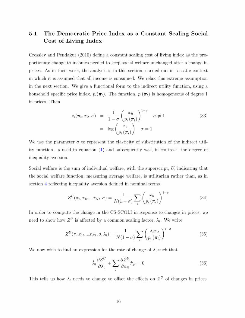
5.1 The Democratic Price Index as a Constant Scaling SocialCost of Living Index

Crossley and Pendakur (2010) define a constant scaling cost of living index as the pro-

portionate change to incomes needed to keep social welfare unchanged after a change in

prices. As in their work, the analysis is in this section, carried out in a static context

in which it is assumed that all income is consumed. We relax this extreme assumption

in the next section. We give a functional form to the indirect utility function, using a

household specific price index, pi(πt). The function, pi(πt) is homogeneous of degree 1

in prices. Then

zi(πt, xit, σ) =1

1− σ

(xit

pi (πt)

)1−σ

σ 6= 1 (33)

= log

(xi

pi (πt)

)σ = 1

We use the parameter σ to represent the elasticity of substitution of the indirect util-

ity function. ρ used in equation (1) and subsequently was, in contrast, the degree of

inequality aversion.

Social welfare is the sum of individual welfare, with the superscript, U, indicating that

the social welfare function, measuring average welfare, is utilitarian rather than, as in

section 4 reflecting inequality aversion defined in nominal terms

ZU(πt, x1t....xNt, σ) =1

N(1− σ)

∑i

(xit

pi (πt)

)1−σ

(34)

In order to compute the change in the CS-SCOLI in response to changes in prices, we

need to show how ZU is affected by a common scaling factor, λt. We write

ZU(π, x1t....xNt, σ, λt) =1

N(1− σ)

∑i

(λtxitpi (πt)

)1−σ

(35)

We now wish to find an expression for the rate of change of λ, such that

λt∂ZU

∂λt+∑j

∂ZU

∂πjtπjt = 0 (36)

This tells us how λt needs to change to offset the effects on ZU of changes in prices.

16

Rearranging,

λt = −∑

j∂ZU

∂πjtπjt

∂ZU

∂λt

(37)

Looking first at the numerator

∑j

∂ZU

∂πjtπjt = − 1

N

∑i

{(λtxitpi (πt)

)1−σ∑j

∂pi (πt)

∂πjt

πjtpi (πt)

}(38)

Since

∂pi (πt)

∂πjt= ωijt and

∑j

ωijtπjtpi (πt)

=pi (πt)

pi (πt)(39)

it follows that ∑j

∂ZU

∂πjtπjt = − 1

N

∑i

(λtxitpi (πt)

)1−σpi (πt)

pi (πt)(40)

where pi (πt) can be interpreted as the Divisia price index specific to household i.

Also∂ZU

∂λt=

1

Nλt

∑i

(λtxitpi (πt)

)1−σ

(41)

so that

λtλt

=

∑i

(λtxitpi(πt)

)1−σpi(πt)pi(πt)∑

i

(λtxitpi(πt)

)1−σ =

∑i

(xit

pi(πt)

)1−σpi(πt)pi(πt)∑

i

(xit

pi(πt)

)1−σ (42)

giving an expression for the rate of growth of the common scaling cost of living index.

The growth in the social cost of living index is a weighted average of each household’s

growth in its price or cost of living index with the weights reflecting each household’s real

consumption raised to the power of 1-σ. If σ = 1 then the growth in each household’s

price index is given equal weight and the growth rate of the constant scaling cost of

living index is the growth rate of the democratic cost of living index described by Prais

(1958).

This analysis is set out in terms of the instantaneous flow of utility derived from con-

sumption, rather than the accural of life-time utility derived from income. The main

focus of this paper has, however, been on the latter. Rather than consider a quantity ana-

logue at this point, we therefore proceed to consider a social welfare function structured

round income. We defer the issue of exploring the quantity analogue to this deflator

17

to the next section where we examine what can be done to structure a price/quantity

system around income rather than consumption.

5.2 Welfare defined over Income

The welfare which accrues from income to each household in any given period is the

sum of the welfare from consumption and that from saving. The former is given by the

indirect utility function as set out above while, if resources are allocated efficiently, the

latter is equal to the product of saving and the marginal utility of money (see equation

(22)). Thus if each household receives a total income of yit of which xit is consumed we

can write the utility accruing from income as

zyi (πt, xit, yit) = zi (πt, xit) + (yit − xit)∂zi(πt, xit)

∂xit(43)

with the superscript y distinguishing it from the indirect utility function in terms of

consumption alone. The corresponding utilitarian social welfare function, ZY , is then

the sum of each individual household’s utility accruing

ZY (πt, x1t...xNt, y1t...yNt) =1

N

∑i

zi (πt, xit) + (yit − xit)∂zi(πt, xit)

∂xit(44)

The difficulty with this is, of course, that the social welfare is a function of each house-

hold’s consumption as well as its income. The degree to which income has to be scaled to

offset any increase in prices depends on what happens to consumption. That, however,

depends on, among other things, expectations of future prices and incomes.

It is, however, possible to make a first order approximation. Equation (43) is a first-order

Taylor expansion of

zit (πt, xit + [yit − xit]) = zi (πt, yit) . (45)

While, with declining marginal utility of consumption, it will understate the utility

accruing to households with high savings rates, there can be little doubt that zi (π, yit) is

better than zi (πt, xit) as an approximation of zyi (πt, xit, yit). The approximate utilitarian

18

income-based social welfare function is therefore

ZY (πt, y1t...yNt, σ) =1

N

∑i

{1

1− σ

(yit

pi (πt)

)1−σ}

; σ 6= 1 (46)

ZY (πt, y1t...yNt, σ) =1

N

∑i

log

(yit

pi (πt)

); σ = 1.

As we showed in the case of the consumption-based welfare function, this leads to a

price index whose growth rate is given as

P Yt

P Yt

=

∑i

(yit

pi(πt)

)1−σpitpit∑

i

(yi

pi(πt)

)1−σ (47)

In order to develop a quantity measure of income growth we transform ZY (πt, y1t...yNt, σ)

into a variable which is homogeneous of degree 1 in total real income as

QYt = ZY

t

11−σ ; σ > 0, σ 6= 1 (48)

QYt = exp(ZY

t ); σ = 1

so that, after taking logs

1

QYt

(∑i

∂QYt

∂yityi +

∑j

∂QYt

∂πjtπjt

)=

1

(1− σ)ZY

(∑i

∂ZY

∂yityit +

∑j

∂ZY

∂πjtπjt

)(49)

=

∑i

{(yit

pi(πt)

)1−σyityit−(

yitpi(πt)

)1−σ∑j∂pi(πt)∂πjt

πjtpi(πt)

}∑

i

(yit

pi(πt)

)1−σUsing equation (39)

1

QYt

(∑i

∂QYt

∂yityit +

∑j

∂QYt

∂πjtπjt

)=

∑i

{(yit

pi(πt)

)1−σyityit−(

yitpi(πt)

)1−σpi(πt)pi(πt)

}∑

i

(yit

pi(πt)

)1−σ (50)

=

∑i q

1−σit

qitqit∑

i q1−σit

where qit = yit/pi (π) is household real income. We can see that this, not surprisingly,

leads to a system of value, volume and price indicators very similar to that found when

the starting point was Atkinson’s inequality aversion. The difference is that the house-

19

hold weights are computed from real household income, while working from Atkinson

inequality aversion yielded weights based on nominal income. From a practical point of

view, weights based on nominal household income can be compiled from a data source

such as a consumer expenditure survey which also provides details of household incomes,

as does, for example the United Kingdom’s Living Costs and Food Survey. It is much

less clear how real income weights could be calculated without either access to a house-

hold panel survey or by means of an econometric model such as that used by Crossley

and Pendakur (2010) or Jorgenson and Slesnick (2014); the first is, in many cases not

practical while the second may, as we noted earlier, not be appealing to government

statistical offices.

Nevertheless, as before, in the special case where σ = 1, all households are given equal

weights, so the distinction between nominal and real weights does not arise, and the

issue of calculating the weights drops away. Layard, Nickell, and Mayraz (2008), on the

basis of a number of surveys of happiness, find values of σ between 1.19 and 1.34 with

an overall estimate of 1.26, suggesting that the assumption of σ = 1 is a reasonable ap-

proximation given the simplicity it brings both to the calculations and to an explanation

of the resulting variables. With the price index defined in this way, the growth in the

volume index is equal to the average of each household’s growth in money income, less

the growth in a price index constructed along the democratic lines suggested by Prais

(1958). The price/quantity index system constructed by giving each household’s growth

experience equal weight can be justified either heuristically as representing a particu-

lar form of inequality aversion, or deduced from a welfare function which is a first-order

approximation to the utility accruing to each household as a result of its current income.

6 A Democratic Measure of Real Household Income

Growth for the United Kingdom

6.1 The Geometric Mean and the Median

Jorgenson and Schreyer (2017) make the point that, if equivalised consumption or in-

come is log-normally distributed, then the median and the geometric mean will co-incide.

In fact this is true if the distribution of log consumption or income takes any symmet-

ric distribution. Figure 1 shows the mean, median and geometric mean of equivalised

20

household income after housing costs taken from the Households Below Average Income

(HBAI) data set (Department of Work and Pensions 2017).3 This shows that, in the

United Kingdom at least, the geometric mean is indeed close to the median. Between

financial years 2005/6 and 2015/6 the nominal geometric mean grew by 32.2 per cent

while the median grew by 33.0 per cent and the mean grew by 33.8 per cent.4 Thus,

over this period, at least, there were material differences in the growth rates of the three

summary measures, notwithstanding the observation that, in level terms, the geometric

mean of income after housing costs was close to the median.

Figure 1: Measures of Central Tendency (£ per week) for UK Equivalised Household Incomesafter Housing Costs (Financial Years)

300

350

400

450

500

550

£ pe

r w

eek

2005 2006 2007 2008 2009 2010 2011 2012 2013 2014 2015

Geometric mean Median

Mean

3Despite the name, HBAI covers the entire population, and not just those below average income.See Appendix C for more details on this, and other data we use.

4The main results we present are computed giving each household its sampling weight in HBAI.However there is a question of how appropriate this is when the geometric mean is used, and we thereforealso present unweighted figures for each of the three measures of real income growth in footnote 5.

21

Figure 2: Growth Rates of the Geometric Mean, Median and Arithmetic Mean of EquivalisedHousehold Income after Housing Costs (Financial Years)

02

46

Per

cen

t per

ann

um

2006 2007 2008 2009 2010 2011 2012 2013 2014 2015 Average

Geometric mean Median

Arithmetic mean

Figure 2 shows the annual growth rates of these three measures of income. There is

no general rule as to which rises most or least, but, averaged over the ten years of the

data set, the geometric mean has grown at an annual rate of 2.83 per cent, the median

at 2.89 per cent and the arithmetic mean at 2.95 per cent per annum. Thus, while in

level terms, the median is fairly close to the geometric mean, in growth rate terms, the

experience of the median household was midway between the two means.

6.2 Plutocratic and Democratic Price Indices

Since early in 2017 the core measure of inflation in the UK, CPIH has included all

housing costs including the imputed rent of owner occupiers; CPI excluding imputed rent

is also published. The Office for National Statistics (2017b) presents a measure which

excludes imputed and actual rent, maintenance costs and water and sewerage charges as

22

the most suitable measure consistent with conventional CPI for deflating income after

housing costs. We use this as our plutocratic price index noting that it is constructed

using consumption weights. Our plutocratic price index therefore corresponds to PC(0)

of section 4.3 rather than P (0) of section 3 because this is the price index in common

use.

The weights needed for a democratic price index have to be taken from household survey

data, while the weights for the plutocratic measure are those of aggregate consumption

patterns as shown in the national accounts. Much work on the production of democratic

price indices has taken survey data as the sole source from which to calculate the weights

for a democratic consumption price index. It is, however, increasingly recognised that

there are material differences between expenditure patterns in households surveys and

those shown in the national accounts. A standard means of addressing this is to scale

survey consumption figures to align them with the national accounts. Thus, for example,

Jorgenson and Schreyer (2017) split consumption into fifteen categories and scale each of

these before they calculate consumption price indices for households in different parts of

the income distribution. Ley (2005) suggests that the difference between the democratic

and the plutocratic price indices is likely to depend on how fine the disaggregation is;

rich and poor may buy similar amounts in broad categories, but buy rather different

goods when fine disaggregations are studied.

The work on which we draw (Office for National Statistics 2017a) identifies eighty-

seven categories of consumption and aligns each of these to the national accounts and

thus to the basis used for calculating the conventional plutocratic consumer price index

before calculating the mean of the household expenditure shares needed to deliver the

democratic price index. The core work in this area led to a price index which included

housing costs with owner occupiers’ costs measured by imputed rent; however the Office

for National Statistics has kindly made available a democratic price index calculated

excluding imputed and actual rent, maintenance costs and water and sewerage charges5

and we have used this as our democratic price index.

Both price indices are chain-linked with the weights updated in every year. There

is, however, a concern that erratic movements in consumption may make the use of

5Available at https://www.ons.gov.uk/economy/inflationandpriceindices/adhocs/007752democraticmeasureofcpihexcludinghousinguk2005to2016

23

weights based on the previous year’s expenditure patterns alone inappropriate. Instead,

therefore, the Office for National Statistics uses the average of the expenditure patterns

of the previous three years to provide the weights.

Figure 3: Democratic and Plutocratic Price Inflation excludingHousing Costs (Financial Years)

01

23

45

Per

cen

t per

ann

um

2006 2007 2008 2009 2010 2011 2012 2013 2014 2015 Average

Democratic price index Plutocratic price index

The annual rates of growth of the two indices are shown in figure 3. Over the ten years

from financial year 2005/6 to financial year 2015/6, the democratic price index grew at

an average rate of 2.63 per cent per annum while the plutocratic counterpart grew at

2.42 per cent per annum. This difference is well within the range of divergence reported

by Ley (2005).

24

6.3 A Democratic Measure of Equivalised Household Real In-come Growth

Figure 4 shows the measures of real income growth calculated from the geometric mean

deflated by the democratic price index and the arithmetic mean deflated by the pluto-

cratic price index. The discrepancies in the nominal growth rates are augmented by the

differences in the movements of the deflators so, over the ten-year period democratic real

household income has grown at 0.20 per cent per annum while plutocratic real household

income has grown by 0.52 per cent per annum, and median household income deflated

by the plutocratic price index (not shown) has grown at 0.46 per cent per annum.6 Thus,

deflated by the plutocratic price index, growth of median income would give a rather

misleading view of the real income growth experience of the average household.

7 Conclusions

This article suggests a practical means by which statistical offices can produce indicators

of economic growth which are sensitive to changes in the distribution of resources. Our

approach is to focus on the average growth experience of each household. Thus, while

the measure points to a focus on the geometric mean rather than the arithmetic mean of

real incomes, it can be explained straightforwardly as treating each household’s income

growth experience equally. We demonstrate that the democratic price index proposed

by Prais (1958) is the natural deflator to be applied to the geometric mean. We show

that this can be derived from inequality aversion of the type proposed by Atkinson

(1970) with the degree of inequality aversion set equal to 1, decomposing the nominal

aggregate which results into quantity and price terms. We describe the growth in the

quantity indicator as a democratic indicator of household real income growth because

each household’s experience counts equally. While the same approach can be used with

degrees of inequality aversion different from one, household-specific weights enter into

the calculations raising practical problems if, for example, income and expenditure data

are taken from different sources as in the example we present here.

We show that, when capital accumulation is the sole source of income growth, growth

6The real growth rates calculated from the unweighted arithmetic mean, median and geometricmean respectively are: 0.38% p.a., 0.42% p.a. and 0.13% p.a. As before the first two are calculatedusing the plutocratic price index and the last is deflated using the democratic price index.

25

Figure 4: Growth Rates of Real Democratic and Plutocratic Equivalised Household Incomeafter Housing Costs (Financial Years)

-4-2

02

4P

er c

ent p

er a

nnum

2006 2007 2008 2009 2010 2011 2012 2013 2014 2015 Average

Real Democratic income Real Plutocratic income

in the quantity indicator can be given an interpretation in terms of growth in life-time

utility measured relative to each household’s income valued at the marginal utility of

money. This contrasts with the conventional measure of real income growth which

measures each household’s growth in utility with reference to average income, reducing

the importance given to growth in utility of households with low incomes.

Finally we show that the democratic price index can be seen as a constant scaling social

cost of living index for a set of household with homothetic but not homogenous pref-

erences and with logarithmic utility functions. Making use of existing results on the

interpretation of saving we show that to a first approximation, the constant scaling cost

of living index approach provides a framework which, with logarithmic utility, deliv-

ers the price/quantity breakdown obtained directly from Atkinson inequality aversion.

International empirical evidence suggests that the assumption of logarithmic utility is

a reasonable approximation. This suggests that a democratic measure of real income

26

growth could be used as an indicator of welfare change which can be explained straight-

forwardly to non-technical users.

Calculations for the United Kingdom suggest both that the arithmetic mean of income

rose faster than the geometric mean and that the democratic price index rose faster

than the plutocratic price index. Taking these two together, a plutocratic measure of

household income rose at an annual rate of 0.32% per annum faster than a democratic

measure over the ten years from 2005.

27

8 References

Atkinson, A.B. 1970. “On the Measurement of Inequality.” Journal of Economic Theory

2:244–263.

Balk, B.M. 1995. “Axiomatic Price Index Theory: a Survey.” International Statistical

Review 63:69–93.

Crossley, T.F. and K. Pendakur. 2010. “The Common-Scaling Social Cost-of-Living

Index.” Journal of Business and Economic Statistics 28:523–538.

Department of Work and Pensions. 2017. “Households Below Average Income: 1994/95-

2015/16.” 10th Edition. UK Data Service. SN 5828. http://doi.org/10.5255/UKDA-

SN-5828-8.

Jorgenson, D.S. and D.T. Slesnick. 2014. “Measuring Social Welfare in the U.S. National

Accounts.” In Measuring Economic Sustainability and Progress, edited by D.W. Jor-

genson, J.S. Landefeld, and P. Schreyer. Chicago: University of Chicago Press, 43–88.

Jorgenson, D.W. 1990. “Aggregate Consumer Behaviour and the Measurement of Social

Welfare.” Econometrica 58:1007–1040.

Jorgenson, D.W. and P. Schreyer. 2017. “Measuring Individual Economic Well-Being

and Social Welfare within the Framework of the System of National Accounts.” Review

of Income and Wealth 63:S460–S477.

Jorgenson, D.W. and D.T. Slesnick. 1983. “Aggregate Consumer Behaviour and the

Measurement of Inequality.” Review of Economic Studies 51:369–392.

Kehoe, T.J. and D.K. Levine. 1990. “Determinacy of Equilibria in Dynamic Models

with Finitely Many Consumers.” Journal of Economic Theory 50:1–21.

Layard, R., S. Nickell, and G. Mayraz. 2008. “The Marginal Utility of Income.” Journal

of Public Economics 92:1846–1857.

Ley, E. 2005. “Whose Inflation? A Characterisation of the CPI Plutocratic Gap.” Oxford

Economic Papers 57:634–646.

Newbery, D.M. 1995. “The Distributional Impact of Price Changes in Hungary and the

United Kingdom.” Economic Journal 105:847–863.

28

Office for National Statistics. 2017a. “Investigating the

Impact of Different Weighting Methods on CPIH.”

Https://www.ons.gov.uk/economy/inflationandpriceindices/methodologies/ in-

vestigatingtheimpactofdifferentweightingmethodsoncpih.

———. 2017b. “Wealth and Assets Survey, Waves 1-4.” 5th Edition. UK Data Service.

SN: 7215, http://doi.org/10.5255/UKDA-SN-7215-5.

Organisation for Economic Co-operation and Development. 2011. “What are Equivalence

Scales?” Http://www.oecd.org/els/soc/OECD-Note-EquivalenceScales.pdf.

Oulton, N. 2008. “Chain Indices of the Cost of Living and the Path-Dependence Problem:

a Proposed Solution.” Journal of Econometrics 144:306–324.

Pollak, R. 1981. “The Social Cost of Living Index.” Journal of Public Economics

15:311–336.

Prais, S. 1958. “Whose Cost of Living?” Review of Economics and Statistics 26:126–134.

Redding, S.J. and D.E. Weinstein. 2016. “A Unified Approach to Estimating Demand.”

CEP Disucssion Paper No 1445.

Samuelson, P.A. and S. Swamy. 1974. “Invariant Economic Index Numbers and Canon-

ical Duality: Survey and Synthesis.” American Economic Review 64:566–593.

Sefton, J. and M.R. Weale. 2006. “The Concept of Income in a General Equilibrium.”

Review of Economic Studies 73:219–249.

Slesnick, D.T. 1998. “Empirical Approaches to the Measurement of Welfare.” Journal

of Economic Literature 36:2108–2165.

Stiglitz, J, A. Sen, and J-P Fitoussi. 2009. Report by the Commission on the Measure-

ment of Economic Performance and Social Progress. Paris: INSEE.

Weitzman, M. 1976. “On the Welfare Significance of National Product in a Dynamic

Economy.” Quarterly Journal of Economics 90:156–162.

29

A Demand Shifts and the Divisia Index

This appendix provides an example which shows how the Divisia index can be robust

to changes in the mix of demand arising as a result of demand shifts as well as price

changes. We assume that utility is given by a constant elasticity of substitution utility

function

ui =

(∑(cijψij

)1−σ) 1

1−σ

σ > 0; σ 6= 1 (51)

Here ψij are the demand parameters which are specific to household i and time-varying.

The associated price index is then given as

pσ−1σ

i =∑j

(πjψij)σ−1σ (52)

The associated expenditure shares are

ωij =(πjψij)

σ−1σ∑

j(πjψij)σ−1σ

(53)

Differentiating (52) yields

dpipip1−σi =

∑j

dπjπj

(πjψij)1−σ +

∑j

dψijψij

(πjψij)1−σ (54)

so thatdpipi

=∑j

ωijdπjπj

+∑j

ωijdψijψij

(55)

The condition for the Divisia index to be valid for household i is therefore∑j

ωijdψijψij

= 0 (56)

The proportionate rates of change in the demand parameters, weighted by the associated

expenditure shares, have to sum to zero.

30

B Welfare and Aggregate Income

We start with the definition of aggregate real income, using the superscript C because the

underlying price deflator is calculated using shares of total consumption, weighting each

household’s consumption shares by its total consumption rather than its total income.

In this calculation zero inequality aversion is assumed

QCt (0) =

∑i pitqitPCt (0)

(57)

where the aggregate price index is defined as

PCt (0)

PCt (0)

=∑i

π′tcit∑i,j π

′tcit

pitpit. (58)

The rate of change of QCt (0) is

QCt (0) =

∑i

{pitPCt

qit +qitPCt

pit

}− PC

t

PCt

∑i pitqitPCt

(59)

We now substitute qit = rit(qit − π′tcit/pit) + hit to give

QCt (0) =

∑i

{pit

PCt (0)

qit +rit(qit − π′tcit/pit) + hit

PCt (0)

pit

}− PC

t (0)

PCt (0)

∑i pitqitPCt (0)

(60)

First we note that ∑i

ritπ′tcit/pit

PCt (0)

pit = rtCt

where Ct is an index of aggregate consumption measured as Ct = π′tct/PCt (0) and rt is

the aggregate real rate of interest defined as the nominal rate of interest less the rate of

growth of the aggregate consumption price index. rt = r∗t −PCt (0)

PCt (0). For a proof of this see

Sefton and Weale (2006), pp 245-246. We can then write (60), putting Ht =∑

ipithitPCt (0)

31

as the exogenous contribution to aggregate growth

QCt (0) =

∑i

{pit

PCt (0)

+ritpitPCt (0)

− PCt (0)

PCt (0)

pitPCt (0)

}qit − rtCt +Ht (61)

=∑i

{pit

PCt (0)

+(r∗t − pit/pit) pit

PCt (0)

− PCt (0)

PCt (0)

pitPCt (0)

}qit − rtCt +Ht

=∑i

{r∗t pitPCt (0)

− PCt (0)

PCt (0)

pitPCt (0)

}qit − rtCt +Ht

=

(r∗t −

PCt (0)

PCt (0)

)∑i

pitqitPCt (0)

− rtCt +Ht

= rt(QCt (0)− Ct

)+Ht

This yields the aggregate equivalent of equation (18). We can integrate it to give

QCt (0) +

∫ ∞t

Hτe−

∫ τt riνdνdτ =

∫ ∞t

rτπ′τcτ/P

Ct e−

∫ τt rνdνdτ (62)

=

∫ ∞t

rτCte−

∫ τt rνdνdτ

showing the relationship between aggregate real income and current and future con-

sumption.

We how turn to the growth in utility starting with the equation for household i

d

dt

∫ ∞t

ui(ciτ )e−θτdτ = pit

∂zit∂xit

∫ ∞t

(riτπ′τciτe

−∫ τt riνdν/piτ )dτ − π′tcit/pit. (63)

Aggregating using the function (26) and then using equation (27)

d

dt

∑i

∫ ∞t

αiui(ciτ )e−θτdτ =

∑i

pitαi∂zit∂xit

∫ ∞t

(riτπ′τciτe

−∫ τt riνdν/piτ )dτ − π′tcit/pit

=∂ZM

∂Xt

∑i

pit

∫ ∞t

(riτπ′τciτe

−∫ τt riνdν/piτ )dτ − π′tcit/pit

=∂ZM

∂Xt

∑i

pit

∫ ∞t

(riτπ′τciτe

−∫ τt riνdν/piτ )dτ − π′tcit/pit

= PCt (0)

∂ZM

∂Xt

(QCt (0) +

∫ ∞t

Hτe−

∫ τt rνdνdτ − Ct

)(64)

32

From this it follows that

QCt (0)− Ct =

1

PCt ∂Z

M/∂Xt

d

dt

∑i

∫ ∞t

αiui(ciτ )e−θτdτ − rt

∫ ∞t

Hτe−

∫ τt rνdνdτ (65)

and therefore that

QC(0)

QCt (0)

=rt

PCt (0)QC

t (0)∂ZM/∂Xt

d

dt

∑i

∫ ∞t

αiui(ciτ )e−θτdτ +

Ht − rt∫∞tHτe

−∫ τt rνdνdτ

QCt (0)

=rt

Yt∂ZM/∂Xt

d

dt

∑i

∫ ∞t

αiui(ciτ )e−θτdτ +

Ht − rt∫∞tHτe

−∫ τt rνdνdτ

QCt (0)

(66)

As with the democratic measure of income growth, there are two components. The

first shows the dividend earned on the increase in the social welfare function, measured

relative to aggregate money income multiplied by the marginal utility of money. But ag-

gregate social welfare is the weighted sum of individual utility. Each household’s weight

is inversely proportional to its marginal utility of consumption and thus increase in the

welfare of households with high marginal utility and therefore low utility is downweighted

as compared to households with low marginal and high absolute utility.

C Data Appendix

The democratic price index we have used is available from Democratic price index and

the plutocratic price index from Plutocratic price index.

In both cases we have calculated price indices for financial years (April to March) as the

arithmetic averages of the relevant monthly data.

HBAI (Households Below Average Income) data are derived from the Family Resources

Survey (FRS), a representative annual sample of about 20,000 private households in

the UK. From the HBAI we use the household net income after housing costs variable

esahcohh. The data are adjusted for household size and composition by equivalisation

using the rescaled modifed OECD scale (variable eqoahchh). Income is adjusted in the

HBAI for undercoverage of top incomes by using replacement values from the Survey

of Personal Incomes (SPI). As with any survey, HBAI data are at risk from systematic

bias due to non-response by households selected for interview in the FRS. In an attempt

to correct for differential non-response, estimates are weighted using population totals.

33

The analysis is conducted at the household level, and therefore the data are weighted

using the household weight gs newhh.

34