
A Decision Support System for real-time track assignment ...
79
A Decision Support System for real-time track assignment at railway yards Master Thesis for the written by Bram B. W. Schasfoort (born June 9th, 1994 in Hilversum, Netherlands) at Date of the public defense: Members of the Thesis Committee: July 5th, 2019 Prof. Dr. Ir. Eric van Berkum Dr. Kostantinos Gkiotilitis Vincent den Ouden, MSc
Transcript of A Decision Support System for real-time track assignment ...

A Decision Support System for real-timetrack assignment at railway yards
Master Thesisfor the
written by
Bram B. W. Schasfoort(born June 9th, 1994 in Hilversum, Netherlands)
at
Date of the public defense: Members of the Thesis Committee:July 5th, 2019 Prof. Dr. Ir. Eric van Berkum
Dr. Kostantinos GkiotilitisVincent den Ouden, MSc

II

Abstract
English
In this thesis, we study the Real-Time Track Assignment Problem (RT-TAP), a real-time assignmentproblem that arises from the high percentage of stochastic arrivals of freight trains and the largequantity of last-minute parking requests at railway yards. We show that the RT-TAP is NP-Hard andprovide a mixed integer program for solving the RT-TAP by minimizing the total weighted delay oftrains. Because of its computational complexity, we develop a problem specific Genetic Algorithm(GA) and compare it with a First Scheduled First Served (FSFS) heuristic. Smaller instances showthat there is no optimality gap between the Brute Force (BF) approach and the GA. The heuristicapproaches are tested on two Real-Time simulations where we consider 74 inbound trains and 9tracks. In order to define the effect of the input on the two models, we excluded in one of thesimulations the track length i.e. all trains can be assigned to all tracks. Although we saw that theoutput of the GA remained the same, the FSFS heuristic was not able to show results as good asthe GA. Therefore, we conclude that we developed a Decision Support System (DSS) that cannotonly stabilize, but also improve the current decision-making process with regards to real-time trackassignment at railway yards.
Keywords: Track Assignment; Real-Time; Rail Operations; Minimizing delays; Scheduling.
Nederlands
In deze scriptie bestuderen we het realtime spoor toewijzingsprobleem (RT-TAP), een probleemdat ontstaat door het hoge percentage van stochastische aankomsten van goederentreinen en hetgrote hoeveelheid last-minute parkeerverzoeken op emplacementen. We laten zien dat het RT-TAPNP-hard is en ontwikkelen een mixed integer program gemaakt voor het oplossen van het RT-TAPdoor de totale gewogen vertraging van treinen te minimaliseren. Vanwege de computationele com-plexiteit ontwikkelen we een probleemspecifiek Genetisch Algorithme (GA) en vergelijken deze meteen First Scheduled First Served (FSFS) heuristiek. Bij het testen van kleinere scenario’s tonenwe aan dat er geen optimaliteitskloof is tussen een Brute Force (BF) benadering en het GA. Detwee heuristieken worden getest op twee realtime simulaties met 74 inkomende treinen en 9 sporen.Om het effect van de invoer op de twee modellen te definieren, hebben we in een van de simu-laties de spoorlengte uitgesloten, d.w.z. alle treinen kunnen aan alle sporen worden toegewezen.Hoewel we zagen dat de resultaten van het GA hetzelfde bleven, had de FSFS heuristiek moeite methet produceren van even goede resultaten Daarom concluderen we dat we succesvol een beslissing-sondersteuningssysteem (DSS) hebben ontwikkeld die niet alleen het huidige besluitvormingsprocesmet betrekking tot realtime spoortoewijzing kan stabiliseren, maar ook kan verbeteren.
Trefwoorden: Spoortoewijzing; Realtime; Spoorvervoer; Vertragingen minimaliseren; Planning.
iii

IV ABSTRACT

Preface
The thesis on hand marks another milestone, which is the completion of the Master in Civil Engi-neering and Management. The research itself consisted of 7 months of hard work and dedication tothe subjects of railway operations and mathematical optimization. The report is the result of a studyabout a Decision Support System for Real-Time track assignment at railway yards. Interestingly,when I started with this research at Arcadis, I can honestly say that my knowledge about railwayoperations and mathematical modeling was very limited. Nonetheless, the reason that everythingwas very new to me, was probably one of the biggest reasons that the subject remained interested,all the way to the end. I can therefore summarize this last period as one big learning experience,which I enjoyed a lot!!
Of course, achieving something like this was not without help. Therefore, I would hereby like toshow my sincere gratitude to the following people whom without this project would not have beenpossible.
Konstantinos Gkiotsalitis,My UT supervisor who without his dedications and the amount of energy he put in this project, I wouldnever have been able to achieve the quality that I present you in this thesis! I highly appreciated thespeed you provided me feedback and the time you took during the meetings to discuss every matter.
Vincent den Ouden,My supervisor from Arcadis who always would find a moment to take the time and discuss everythingthat was going on with this project. Furthermore, I would like to thank you for giving me the freedom,that I probably also needed, during this research to use my own approaches. Heel erg bedankt!
I would like to give a special thank you to my brother Job Schasfoort , who helped me greatlywith learning and understanding the C++ programming language, Oskar Eikenbroek for helpingme with the development of the methodology, and Andre van Es who arranged the opportunityto do my graduation at Arcadis. Further, I would like to thank my parents Adele Veldboer andEgbert Schasfoort for their support and encouragement during my whole study period, starting withthe MBO, Bachelor, and eventually also this Master! Finally, a big thanks to all the nice colleaguesfrom Arcadis including the football table on the third floor for all the inspirational moments, ProRail formaking the data available for me to use during the numerical experiment, and everybody who I didnot mention yet and supported me during the whole thesis process.
Hope you enjoy!
Bram Schasfoort,
Enschede, June 11th, 2019
v

VI PREFACE

Contents
Abstract iii
Preface v
List of Figures ix
List of Tables xi
List of acronyms xiii
1 Introduction 1
2 Related Studies 5
3 Research Gap, Aim & Relevance 73.1 Research gap & context . . . . . . . . . . . . . . . . . . . . . . . . . . . . . . . . . . . 73.2 Research aim . . . . . . . . . . . . . . . . . . . . . . . . . . . . . . . . . . . . . . . . . 83.3 Contribution of this Thesis . . . . . . . . . . . . . . . . . . . . . . . . . . . . . . . . . . 8
4 Methodology 114.1 Overall framework . . . . . . . . . . . . . . . . . . . . . . . . . . . . . . . . . . . . . . 124.2 Feasibility set . . . . . . . . . . . . . . . . . . . . . . . . . . . . . . . . . . . . . . . . . 164.3 Computational complexity . . . . . . . . . . . . . . . . . . . . . . . . . . . . . . . . . . 194.4 Mathematical program . . . . . . . . . . . . . . . . . . . . . . . . . . . . . . . . . . . . 20
5 Solution Method 215.1 Brute Force solution method . . . . . . . . . . . . . . . . . . . . . . . . . . . . . . . . 215.2 Problem specific Genetic Algorithm . . . . . . . . . . . . . . . . . . . . . . . . . . . . . 235.3 First Scheduled First Served approach . . . . . . . . . . . . . . . . . . . . . . . . . . . 26
6 Numerical Experiment 276.1 Case study description . . . . . . . . . . . . . . . . . . . . . . . . . . . . . . . . . . . . 276.2 Numerical input received and assumptions made . . . . . . . . . . . . . . . . . . . . . 286.3 Sensitivity analysis on hyper-parameters . . . . . . . . . . . . . . . . . . . . . . . . . . 336.4 Description of the benchmark . . . . . . . . . . . . . . . . . . . . . . . . . . . . . . . . 366.5 Computational results . . . . . . . . . . . . . . . . . . . . . . . . . . . . . . . . . . . . 37
6.5.1 Performance on smaller instances . . . . . . . . . . . . . . . . . . . . . . . . . 376.5.2 Real-time simulation of the model without considering train lengths . . . . . . . 386.5.3 Real-time simulation of the model with track length limitations . . . . . . . . . . 396.5.4 Estimating the trains’ arrival . . . . . . . . . . . . . . . . . . . . . . . . . . . . . 39
vii

VIII CONTENTS
6.6 Exploitation of the local optima . . . . . . . . . . . . . . . . . . . . . . . . . . . . . . . 40
7 Discussion 41
8 Conclusion 45
References 47
Appendices
A MOD file of the AMPL model 51
B DATA file of the AMPL model 53
C RUN file of the AMPL model 55
D Overview drawing of Waalhaven Zuid 57
E Determining process times of trains 59
F Generating Length 61
G Delay distribution of trains 63

List of Figures
4.1 Visualization of the problem . . . . . . . . . . . . . . . . . . . . . . . . . . . . . . . . . 114.2 Schematic layout of the assignment situation . . . . . . . . . . . . . . . . . . . . . . . 124.3 Visualization of the sequential problem where each sequence represents a track as-
signment, the square represents the beginning and end of each sequence, and eachcircle represents a train . . . . . . . . . . . . . . . . . . . . . . . . . . . . . . . . . . . 13
4.4 Arrival sequence of train i and j at track k . . . . . . . . . . . . . . . . . . . . . . . . . 164.5 Example of sub tours that will be eliminated by using equation 4.11 . . . . . . . . . . . 17
6.1 Schematic overview of Waalhaven Zuid process tracks . . . . . . . . . . . . . . . . . . 276.2 Visualization of the process times of each train . . . . . . . . . . . . . . . . . . . . . . 306.3 Visualization of the adjusted original train scheduled used in the experiments . . . . . 316.4 Applied delays from the Original plan to Scheduled plan . . . . . . . . . . . . . . . . . 316.5 Applied delays from the Original plan to Executed . . . . . . . . . . . . . . . . . . . . . 326.6 Visualization of the length of each train . . . . . . . . . . . . . . . . . . . . . . . . . . . 326.7 Four different recombination rates (µ%) (average over five tests) . . . . . . . . . . . . 336.8 Six different mutation rates (average over five tests) . . . . . . . . . . . . . . . . . . . 346.9 Four different population sizes (average over five tests) . . . . . . . . . . . . . . . . . . 356.10 Real-time performance (excluding track length) . . . . . . . . . . . . . . . . . . . . . . 386.11 Real-time performance (including track length limitations) . . . . . . . . . . . . . . . . 396.12 Visualization of train assignments that yield an equivalent performance . . . . . . . . . 40
D.1 Overview drawing of Waalhaven Zuid (Sporenplan, 2016) . . . . . . . . . . . . . . . . 57
E.1 Train number setup of the Dutch railway network . . . . . . . . . . . . . . . . . . . . . 59E.2 Visualization of the original train scheduled . . . . . . . . . . . . . . . . . . . . . . . . 60
G.1 Delay distribution on arrivals of trains (original compared with executed data) . . . . . 64G.2 Delay distribution on arrivals of trains (planned compared with executed data) . . . . . 64G.3 Stochastic optimization excluding the length of trains for 6 am (left) and 10 am (right) . 65G.4 Stochastic optimization including the length of trains for 6 am (left) and 10 am (right) . 65
ix

X LIST OF FIGURES
List of Tables
1.1 Delays of freight trains; original compared to executed data at Waalhaven Zuid (Pro-Rail, 2015) . . . . . . . . . . . . . . . . . . . . . . . . . . . . . . . . . . . . . . . . . . 2
1.2 Executed trains from predetermined plan at Waalhaven Zuid (ProRail, 2015) . . . . . 2
4.1 General subscripts . . . . . . . . . . . . . . . . . . . . . . . . . . . . . . . . . . . . . . 154.2 Parameters . . . . . . . . . . . . . . . . . . . . . . . . . . . . . . . . . . . . . . . . . . 154.3 Variables . . . . . . . . . . . . . . . . . . . . . . . . . . . . . . . . . . . . . . . . . . . 154.4 Decision variables . . . . . . . . . . . . . . . . . . . . . . . . . . . . . . . . . . . . . . 15
5.1 Removing double member from the solution space. . . . . . . . . . . . . . . . . . . . . 25
6.1 Data necessary for the model based on the mathematical model . . . . . . . . . . . . 286.2 Arrival distribution over the week (ProRail, 2015) . . . . . . . . . . . . . . . . . . . . . 306.3 Results when applying different recombination rates . . . . . . . . . . . . . . . . . . . 336.4 Results of the five test for each different mutation rates . . . . . . . . . . . . . . . . . . 346.5 Results with different population sizes . . . . . . . . . . . . . . . . . . . . . . . . . . . 356.6 Comparison of the CPLEX optimization, the First Scheduled First Served algorithm,
and the Genetic Algorithm . . . . . . . . . . . . . . . . . . . . . . . . . . . . . . . . . . 37
E.1 Processes when arriving at Waalhaven Zuid from the network and departing to RailService Center . . . . . . . . . . . . . . . . . . . . . . . . . . . . . . . . . . . . . . . . 60
E.2 Processes when departing from Waalhaven Zuid after visiting Rail Service Center . . 60
G.1 Trains’ delay, mean values and variances . . . . . . . . . . . . . . . . . . . . . . . . . 63
xi

XII LIST OF TABLES

List of acronyms
ARS Automatic Route Setting
BF Brute Force method
CBG Centraal Bediend Gebied
DSS Decision Support System
DY Destination Yard
FIFO First In First Out
FSFS First Scheduled First Served
GA Genetic Algorithm
HC Hill Climbing
LIFO Last In First Out
RIM Rail Infrastructure Manager
RRT Railcar Retrieval Problem
RSC Rail Service Center
RT-TAP Real-Time Track Assignment Problem
SA Simulated Annealing
TAP Train Assignment Problem
TD Train Dispatcher
TS Tabu Search
TUSP Train Unit Shunting Problem
TY Temporary Yard
VRP Vehicle Routing Problem
Whz Waalhaven Zuid
xiii

XIV LIST OF ACRONYMS

Chapter 1
Introduction
Since the use of the first railway in the early 19th century, rail freight transportation has alwaysplayed an important role in the transportation sector (Network Rail, 2016). As discussed by Givoniand Banister (2013), after long and short haul maritime transport is, rail freight transport is the modewith the least CO2 emission per kg/tonne-km.
While the rail transportation sector is still growing, the increase in demand could cause capacityproblems on the network. For example, US transportation officials already stated their concerns thatfuture capacity limitations of the American railway system are likely to result in a degradation of speedand reliability of the network (U.S. Railroad, 2008). While a need for further expansion of railway net-works is strongly desired around the globe, the most common solution would be an expansion of therailway network by constructing new infrastructure. However, constructing new infrastructure is gen-erally decided by policymakers and involves a long-term decision process including large expenses(Boysen et al., 2012; Narayanaswami and Rangaraj, 2011). Because of high construction costs, itmight be better to increase the occupancy and transit rate on the network in order to comply with theincrease of traffic.
In order to comply with the demand for rail freight transporters, timetables of trains are determinedone year in advance depending on the country. When a train is driving according to its schedule, theAutomatic Route Setting (ARS) automatically assigns a train to a track (Pachl, 2004). Ideally, a TrainDispatcher (TD), who is responsible for the movement of trains in an assigned area (for example arailway yard), only needs to intervene when unplanned events occur. As discussed by Piner andCondry (2017), there is a possibility that unplanned events result in disturbances and/or disruptions.Now, when a delayed freight train arrives at a railway yard, the track needs to be assigned manuallyby the TD (D’Ariano, 2015; Josyula et al., 2018). Because of the large complexity of optimally as-signing trains to tracks, one can imagine that planning delayed trains at real-time is very complicatedespecially when inexperienced TDs are involved (U.S. Department of Transportation, 1999).
When considering the arrival times of rail freight trains in Europe, it appears that 67% arrives withina 15-minute time frame of their original schedule. Furthermore, 19% of the trains were more than 3hours delayed, and 4% arrived even after 24 hours or their original schedule (European Commission,2014). Concerning the Netherlands, historical data from ProRail (2015) shows that 33% of the trainsthat are originally planned trains arrive within a ± 5-minute time frame of a train’s original plannedtime at their destination yard. 48% of the trains arrive more than 5 minutes later than originallyscheduled, where 26% and 15% of these trains arrive even more than one and two hours too laterespectively (see table 1.1).
1

2 CHAPTER 1. INTRODUCTION
Table 1.1: Delays of freight trains; original compared to executed data at Waalhaven Zuid (ProRail,2015)
Too early (in min) On time Too late (in min) Totals+60 60 - 30 30 - 5 -5 to +5 5 - 30 30 - 60 60 - 120 +120
# of trains 16 8 25 85 40 18 28 40 260
Percentage 6% 3% 10% 33% 15% 7% 11% 15% 100%
Totals : 19% too early 33% 48% too late
Large deviations in arrivals are likely to be related to the fact that rail freight is a part of a supplychain that also includes other modes such as ship and truck transportation. If one of these modes isdelayed, it might cause a knock-on delay on the train that is waiting for its cargo. This could meanthat the freight train leaves the yard already with a delay. Furthermore, when focusing on the distancetraveled by freight trains, most of them are likely to cross borders of different countries resulting inlong distance transport.
When we consider the performance of freight trains on any railway network, we also need toconsider the other rail users. This means that if a train is delayed, it needs to drive in between othertrains without influencing the other users’ schedule. The complexity arises because this train has toperform on the mixed network including the different characteristics of other trains such as speed,acceleration, deceleration, and cargo. When a train is delayed, it can be temporarily stored on a sidetrack so that the train that drives on time can pass. In addition, this later statement together withthat trains need to travel long distances explains the large percentage of trains that have more thantwo or three hours of delay when arriving at their destination (Timmermans, 2018). As substantiatedby Briggs and Beck (2007), delays typically follow an exponential distribution. Because of the highpercentage and the high variance of delays, changing the assignment of freight trains at the executionphase is not a trivial task and is therefore related to the experience and adequate handling of the TD.
To add further complexity to the assignment process, high fluctuation on demand from the clientside results in a late notice of trains requesting paths. For example, table 1.2 shows that 66% ofthe executed trains are planned one year in advance, i.e their arrival is known a year in advance.90% of the executed trains is known when making the original planning, which is done 3 days beforeexecution. This latter means that 10% of the trains will make a request at the last minute whetherthey can park at the yard.
Table 1.2: Executed trains from predetermined plan at Waalhaven Zuid (ProRail, 2015)
Year plan Original plan Scheduled plan Executed# of trains 389 515 573 573
Percentage 66% 90% 100% 100%
The large delays on the network and the high percentage of last-minute requests contribute tothe complexity of assigning trains to tracks at real-time, further referred to as the Real-Time TrackAssignment Problem (RT-TAP). If a suitable fit is not possible, inbound trains might need to wait orbe rerouted to another railway yard, which can result in larger delays. In addition, the large delays oftrains, and the high percentage of trains scheduled with a small prior notice underscores the numberof manual decisions made at railway yards and therefore highlights the need for a Decision SupportSystem (DSS) for the allocation of trains to track at real-time.

3
To tackle this issue, this study models the RT-TAP and investigates mathematical optimizationtechniques that aim to minimize the total delays of outbound trains at a railway yard. The input of themodel is the set of tracks and trains. The set of tracks includes the track number and its correspondinglength. The set of trains incorporate the length of the train, planned arrival and departure time, thetime that the train needs to spend at the yard, and a train weighting. The train weighting is related tothe train’s schedule in relation to the schedule of other trains, the type of train, or the type of cargo(U.S. Department of Transportation, 1999). The output of the model provides an optimal solutionon which track each train should be assigned to in order to minimize the total weighted delay onoutbound trains from the railway yard. The TD can make the final decision based on the outputgenerated by the proposed DSS.
The remainder of this study is structured as follows. In chapter 2 we provide a summary of therelevant literature. After this, we identify the research gap, explain the research goal, and discussthe main contributions of this thesis with regards to the state-of-the-art in chapter 3. Chapter 4describes the overall framework and introduces the mathematical program for solving the RT-TAP byusing a CPLEX solver. Building upon this, we discuss three different solution methods for solvingthe RT-TAP in chapter 5. First, we will explain a Brute Force (BF) approach to solve the problem forsmaller instances. For larger instances, we will introduce a problem specific Genetic Algorithm (GA),and a First Scheduled First Served (FSFS) heuristic solution method. In chapter 6, we providea Numerical Experiment on smaller instances to determine the optimality gap between the threedeveloped solution algorithms. Furthermore, we will show a real-time experiment on a railway yardin the western part of the Netherlands named Waalhaven Zuid based on historical data provided bythe Rail Infrastructure Manager (RIM) of the Netherlands. Finally, discussions and conclusions areoutlined in chapter 7 and 8 respectively.

4 CHAPTER 1. INTRODUCTION
Chapter 2
Related Studies
This section aims to describe the current literature available in the field of railway operations with re-gards to minimizing the total weighted delays, train rescheduling and rerouting, and decision-makingprocesses in real-time control.
Train rescheduling & rerouting decision making
Scheduling is a decision-making process that involves identifying, assessing and making appropri-ate decisions to solve a problem (Josyula et al., 2018) with a goal to optimize one or more objec-tives (Pinedo, 2016). Mathematical approaches for scheduling problems in railway networks areextensively studied. With regards to track assignment problems, most works consider sorting andscheduling problems at marshaling or shunting yards, such as Hansmann and Zimmermann (2008).Shunting movements can be described as the process where a unit is driven to a depot track froma platform in the station and is induced whenever the train composition changes on successive trainservices (Boysen et al., 2012; Gatto et al., 2009; Haahr and Lusby, 2017).
Jaehn et al. (2018, 2015) describes the assignment problems including shunting operations as theRailcar Retrieval Problem (RRT). With this problem, each freight car receives a priority value whichis linked with the due date of each outbound train. The main objective of this problem is to minimizethe total shunting operation costs by minimizing the total weighted departure of all outbound trainsat a shunting yard. Gestrelius et al. (2017) developed an integer programming model for schedulingshunting tasks as well as allocating arrival yard tracks and classification bowl tracks. More effectiveschedules can be found, and a variety of characteristics can be optimized, including shunting workeffort, number or cost of tracks, and shunting task start times. Haahr et al. (2017) describes the TrainUnit Shunting Problem (TUSP), which entails assigning train units from a depot or shunting yard toscheduled train service in such a way that the resulting operations are without conflict. An importantconstraint from the TUSP is that all tracks must be processed in Last In First Out (LIFO) order, whichmeans that trains can only enter from one side of the yard. The Train Assignment Problem (TAP) is todetermine the maximum number of trains that can be assigned to a yard according to the timetableand without the use of shunting. Gilg et al. (2018) shows that the TAP is NP-hard and presents twointeger programming models for solving this problem. The approach integrates track lengths alongwith the three most common types of yard layouts: First In First Out (FIFO), LIFO, and FREE tracks,where FREE is a combination of both LIFO and FIFO.
5

6 CHAPTER 2. RELATED STUDIES
Minimizing delays is a multidisciplinary problem that is widely discussed in many different fields(Schachtebeck and Schobel, 2008, 2010; Schobel, 2007). A survey on Problem models and solutionsapproached with regards to the rescheduling in railway networks is developed by Fang (2015). Sev-eral works such as Dollevoet et al. (2011) and Schobel (2009) discuss minimizing the total (weighted)delays of trains, and use fast heuristic approaches for solving such problems (Dollevoet and Huisman,2014).
Because the models presented above mostly include tactical planning, arrival times of trainscan be modeled by including a stochastic and robust extension of a model in order to consideruncertainties in the optimization process (Boysen et al., 2012; Briggs and Beck, 2007; Gilg et al.,2018).
Real-time algorithms for rescheduling railway systems
In the previous section we discussed several assignment and retrieval problems, however, mostof them are performed at the tactical level and might therefore not be valid when considering thestochastic arrival rates of trains. Hence, a problem solution method for solving assignment problemsat real-time is therefore required (Cai and Goh, 1994). The works found in the literature mostly consistof real-time optimization models for solving railway networks when disruptions occur (Bettinelli et al.,2017). Cacchiani et al. (2014) presents an overview of recovery models and algorithms for real-timerailway rescheduling. As discussed by Dollevoet et al. (2010), railway disruption management is acombination of three different aspects; timetables, rolling stock and crew. Real-time reschedulingof long-distance high-speed trains in a highly disrupted situation is discussed by Zhan et al. (2015).They developed a Decision Support System (DSS) which found solutions for real-time reschedulingwithin 10 minutes of computation time. Other models developed by Fischettia and Monaci (2017) andCorman et al. (2010) found practical solutions for real-time train rescheduling within seconds. Winterand Zimmermann (2000) developed a heuristic approach that assigns trams to tracks at real-timelevel considering the departure of the trams of the next day. If a global optimum is not found at real-time, trams can be reassigned again afterward in other with comply to the schedule of each tram forthe next day.
The works described above all present models solved at real-time. The time limitation to solvea problem at real-time is not strongly specified. For example, while Fischettia and Monaci (2017)and Corman et al. (2010) tried to find practical solutions within seconds, Zhan et al. (2015) acceptedfinding solutions within 10 minutes of computation time. The real-time application for solving theReal-Time Track Assignment Problem (RT-TAP) is therefore dependent on the time between the lastaccurate arrival update and the actual arrival of a train.

Chapter 3
Research Gap, Aim & Relevance
This chapter highlights the research gap in current literature and states the aim that remains centralin this research. Furthermore, we will justify the relevance of conducting research on this topic bydiscussing it on three different categories.
3.1 Research gap & context
In the previous chapter, we argued relevant literature related to the Real-Time Track AssignmentProblem (RT-TAP). We discussed the many models related to Real-Time rescheduling methods andsaw different approaches for track assignment. While the two models presented by Gilg et al. (2018)and Winter and Zimmermann (2000) were closely related to the RT-TAP, the models presented donot offer an exact solution method for this problem. Problems with the application of this modelpresented by Gilg et al. (2018) are that it is performed at the tactical level and considers the scheduleas fixed. It includes an expected deviation, but at real-time, the arrival and departure times can stillvary. The model presented by Winter and Zimmermann (2000) is close to a solution of the RT-TAPas it considers trams to be parked at a yard and includes the arrival and departure time at real-time.However, the model is developed on a single stud yard and focuses on the parking, and not the transitat a yard. Also, when assignments are not optimal, it considers the tram to easily exit the current trackand rearrange a track assignment. Especially the latter is something that should be avoided becauseof the significant length and weight of freight trains. This makes the solution algorithms presentedby Gilg et al. (2018) and Winter and Zimmermann (2000) not suitable as a solution method for theRT-TAP in trains operations.
In this work, we will investigate the RT-TAP and provide a mathematical approach for solving theproblem at hand. Furthermore, we will assess the potentials of using mathematical optimization forallocating freight trains to tracks at any railway yard at real-time.
7

8 CHAPTER 3. RESEARCH GAP, AIM & RELEVANCE
3.2 Research aim
In the previous section, we identified the research gap from existing literature. In this section, wetranslate this gap into a problem definition and state the aim that is central in this research.
Problem definition
Railway operations can deviate from original timetables because of events such as disruptions on thenetwork. For this reason, arrival and departure sequences can change at real-time. Because of thesize of railway yards, they could be perceived as unclear which makes fast decision making difficultand sensitive for mistakes. Furthermore, decisions at real-time are made by a Train Dispatcher (TD)and are dependent on the experience and adequate handling of a TD. Overlap in the schedule couldcause conflict and resolve in more delays on other trains.
Research aim
To develop a fast and easy usable Decision Support System (DSS) that, if delays occur, reassignsinbound trains to tracks in order to minimize the total weighted delays of outbound trains at anyrailway yard at real-time.
3.3 Contribution of this Thesis
This section aims to justify the relevance to conduct a research on this topic. The relevance isdiscussed on three different categories.
Scientific relevance
Ideally, the best-case scenario is that all trains drive according to the original schedule and thereforea TD does not need to intervene at real-time. However, we saw that delayed freight trains performingon the network and last-minute path requests from transportation companies are not exceptional.Currently, the last-minute assignment of trains to tracks is done manually by a TD. Improving themanual allocation of delayed trains with a DSS is, therefore, an interesting field to further investigate.In order to be able to improve this manual decision making, mathematical approaches are alreadywidely discussed in the literature. However, with regards to the research gap stated in section 3.1,we can conclude that the area of assigning delayed trains to tracks when they arrive at an alreadybusy railway yard at real-time is still unexplored. This latter statement is also supported by Gilg et al.(2018), who indicates the limitation of literature with regards to the impact of a trains’ delay on theplanned depot schedules. This said, and considering the large computational complexity of similarexisting track assignment problems, solving such complex problems within a real-time time framewould provide an incremental contribution to the state-of-the-art.
This research will provide insights on real-time track assignment of freight trains and the possibilityof improving the assignment process using mathematical optimization. While manual track assign-ment is non-trivial, the new proposed DSS can be used as a support for a TD for real-time trackassignment at railway yards. In this thesis, an important criterion will be the practical applicability ofthe proposed solution method.

3.3. CONTRIBUTION OF THIS THESIS 9
Social relevance
As stated in the introduction, there is a need for increasing the capacity and transit on any railwaynetwork. However, railway networks are still triggered by large delays. Hoenders (2018) furtheraddresses the relevance of improving network performance when the rail sector would like to continuecompeting with the other freight transportation modes. He points out that there are two options withregard to the large delays on the network; either we try to make sure that trains will drive on time, orwe accept that delays are there and try to make the best of it. While a network without delays wouldbe ideal for the performance because most freight trains cross several borders, and are thereforealso dependent on the network performance of the other countries, reducing delays is not as easyas it sounds. Furthermore, sending out trains that are not fully loaded just to make sure that theydrive on their path is not a good idea. Besides the fact that the transportation companies need tocomply to the demand of the customer, as stated by several rail freight transporters, the profit marginof the trip is on the last wagon of a train (Spoorcafe, 2018). Improving the assignment process andtherefore optimizing the total delay may, therefore, be a much better solution when addressing theproblem within the borders of a country. With all these mentioned reasons above, we can concludethe importance of this research from the social point of view. This statement brings us to the nextsection; the Managerial relevance.
Managerial relevance
The managerial benefit of this research lies in the possibility for Rail Infrastructure Manager (RIM)sto take better-supported decisions concerning real-time track assignment of trains. In the previoussection, we showed that the need for real-time track assignment is there, and is only likely to increaseas more trains will drive on the network. With the large complexity of the current track assignmentproblem, a mathematical approach seems like a good approach in order to improve any inefficienciesat a railway yard with regards to track assignment. The end of the day, the RIM is responsible forscheduling and maintaining the assignments of trains to tracks. In the introduction, we discussed thecomplexity to ensure trains driving within their time slot. No further deterioration or better reducingdelays is important for the overall performance of the supply chain and therefore also the respon-sibility of the RIM. For that reason, using a DSS for assigning trains to tracks at real-time seemslike the only possible solution when considering the process optimization and excluding expensiveconstruction of new infrastructure at railway yards. From a managerial point of view, this research,therefore, shows high relevance when countries, and more specifically the RIMs, want to carry onwith improving the performance of the rail transportation sector and continue to compete with theother modes of freight transportation.

10 CHAPTER 3. RESEARCH GAP, AIM & RELEVANCE

Chapter 4
Methodology
This chapter aims to describe the problem formulation and explains the mathematical program usedfor solving the Real-Time Track Assignment Problem (RT-TAP). In the overall framework, we discussa generalized setup of the problem and explain what kind of input should be provided into the modelin order to make it work properly. The model is eventually tested in the program AMPL by using aCPLEX solver. The three files necessary for executing the model (model, data and the run file) canbe found in appendix A, B and C.
The current situation includes several trains with the same Destination Yard (DY). At this railwayyard, each train needs to perform some sort of operation and therefore must be parked at the yard.These operations could vary from changing the train driver to switching the locomotives of the train.Different operations mean therefore that the minimum time interval a train needs to remain at the DYdiffers per train. The assignment schedule of the trains is shown in figure 4.1. If everything would goaccording to plan, the tactical schedule would be the same as the real-time schedule and no conflictswould occur. However, if the red train receives a delay of 30 minutes, and the green train is stilloperating according to plan, all tracks will be occupied the moment when the black train is plannedto arrive at the yard.
Master Thesis – Bram Schasfoort – Concept 22.05.2019 11
Methodology. This chapter aims to describe the problem formulation and explains the base case scenario of the
model. The base case scenario is a generalized setup of the problem and explains what kind of input
should be provided into the model in order to make it work properly. The model is eventually tested
in the program AMPL using a CPLEX solver. The three files necessary for executing the model
(model, data and the run file) are presented in appendix 1, 2 and 3.
The current situation includes several trains with the same destination yard. At this railway yard,
each train needs to perform some sort of operation and therefore must be parked at the yard. These
operations could vary from changing the train driver to switching the loco motives of the train.
Different operations mean therefore that the minimum time interval a train needs to remain at the
destination yard differs per train. Figure 6.1 shows a time-distance diagram considering six different
trains driving on the network. The assignment order of trains is shown in figure 6.2. If everything
would go according plan, the tactical plan would be the same as the real -time plan and no conflicts
would occur. However, if a delay of 30 minutes is considered on the red train, a conflict will arise
inside the assignment schedule. Because the arrival time of the black train will be earlier than the
departure time of the red train, an overlap in the assignment process will occur. If the red train
would still be assigned at Track 1, it would cause a knock-on delay on the black one and maybe
also the light blue train, which is scheduled to arrive after the black train (See figure 6.1 and 6.2).
Figure 6.1: Time-Distance diagram.
Figure 6.2: Railway yard train assignment diagram.
Destination
Yard (DY)
Time
Dis
tance
Track 1
Track 2
Time
Figure 4.1: Visualization of the problem
11
12 CHAPTER 4. METHODOLOGY
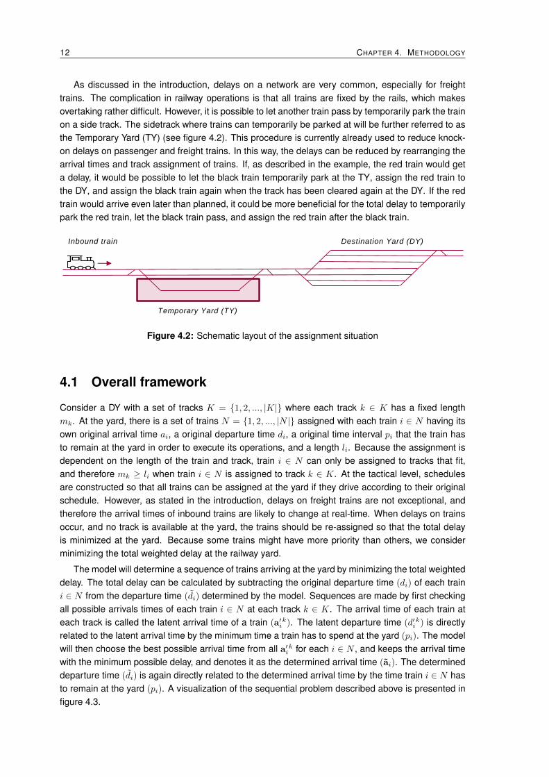
As discussed in the introduction, delays on a network are very common, especially for freighttrains. The complication in railway operations is that all trains are fixed by the rails, which makesovertaking rather difficult. However, it is possible to let another train pass by temporarily park the trainon a side track. The sidetrack where trains can temporarily be parked at will be further referred to asthe Temporary Yard (TY) (see figure 4.2). This procedure is currently already used to reduce knock-on delays on passenger and freight trains. In this way, the delays can be reduced by rearranging thearrival times and track assignment of trains. If, as described in the example, the red train would geta delay, it would be possible to let the black train temporarily park at the TY, assign the red train tothe DY, and assign the black train again when the track has been cleared again at the DY. If the redtrain would arrive even later than planned, it could be more beneficial for the total delay to temporarilypark the red train, let the black train pass, and assign the red train after the black train.
Master Thesis – Bram Schasfoort – Concept 22.05.2019 12
As discussed in the introduction, delays on a network are very common, especially for freight trains.
The complication in railway operations is that all trains are fixed by the rails, which makes
overtaking rather difficult. However, it is possible to let another train pass by temporary park the
first train on a side track. The side track where trains can temporary be parked at will be further
referred as the Temporary Yard (TY) (see figure 6.3). This procedure is currently already used in
the Netherlands to reduce knock-on delays on passenger trains. In this way, the assignment process
can be optimized by rearranging the arrival times and track assignment of trains. If, as described in
the example, the red train would get a delay, it would be possible to le t the black train temporary
park at the TY, assign the red train to the destination yard, and assign the black train again when
the track has been cleared again at the destination yard.
If the red train would get even more delay, it could be more benefici al for the system to temporarily
park the red train, let the black train pass, and assign the red train after the black train.
Overall framework.
Consider a railway yard (destination yard) with a set of tracks 𝐾 = {1,2, … , |𝐾|} where each track 𝑘 ∈
𝐾 has a fixed length 𝑚𝑘. At the yard, there are a set of trains 𝑁 = {1,2, … , |𝑁|} assigned with each
train 𝑛 ∈ 𝑁 having its own scheduled arrival time 𝑎𝑛, a scheduled departure time 𝑑𝑛, a scheduled
time interval 𝑦𝑛 that a train has to remain at the yard in order to perform its operations, and a length
𝑙𝑛 which corresponds with the amount of wagons that a train consists of. Because the assignment is
dependent on the length of the train and track, train 𝑛 ∈ 𝑁 can only be assigned to tracks from the
set 𝐾𝑚𝑖𝑛; 𝑛. This set contains all track 𝑘 that 𝑚𝑘 > 𝑙𝑛 for each train 𝑛. At tactical level, schedules
are determined so that all trains can be assigned at the yard if they drive according to their schedule.
However, as stated in the introduction, because at real -time the arrival times of train can change,
and therefore the amount of trains in need of parking place at time 𝑡 can be higher that the amount
of tracks available. New sequences will therefore be determined by minimizing the total change in
departure time of each train including the trains’ importance, resulting in minimizing the total
weighted delay of all trains.
At real-time the set of 𝑁 trains can be divided into two different categories: (1) Inbound trains, and
(2) parked trains. However, because in practice parked trains can always be moved, no distinction
is made in the model between these two categories. In the model trains have a weighting factor so
that trains that are actually parked at the yard already can be given a high weighting in order to
consider that delaying a parked train would not only cost the time that the train is delayed, but also
the time that the train needs to be moved and parked temporary somewhere else. Besides weighing
parked trains, the factor can also be used to prioritize trains with a tighter schedule than others.
Figure 6.3: Schematic layout of the assignment situation.
Inbound train Destination Yard (DY)
Temporary Yard (TY)
Figure 4.2: Schematic layout of the assignment situation
4.1 Overall framework
Consider a DY with a set of tracks K = {1, 2, ..., |K|} where each track k ∈ K has a fixed lengthmk. At the yard, there is a set of trains N = {1, 2, ..., |N |} assigned with each train i ∈ N having itsown original arrival time ai, a original departure time di, a original time interval pi that the train hasto remain at the yard in order to execute its operations, and a length li. Because the assignment isdependent on the length of the train and track, train i ∈ N can only be assigned to tracks that fit,and therefore mk ≥ li when train i ∈ N is assigned to track k ∈ K. At the tactical level, schedulesare constructed so that all trains can be assigned at the yard if they drive according to their originalschedule. However, as stated in the introduction, delays on freight trains are not exceptional, andtherefore the arrival times of inbound trains are likely to change at real-time. When delays on trainsoccur, and no track is available at the yard, the trains should be re-assigned so that the total delayis minimized at the yard. Because some trains might have more priority than others, we considerminimizing the total weighted delay at the railway yard.
The model will determine a sequence of trains arriving at the yard by minimizing the total weighteddelay. The total delay can be calculated by subtracting the original departure time (di) of each traini ∈ N from the departure time (di) determined by the model. Sequences are made by first checkingall possible arrivals times of each train i ∈ N at each track k ∈ K. The arrival time of each train ateach track is called the latent arrival time of a train (a′i
k). The latent departure time (d′ik) is directly
related to the latent arrival time by the minimum time a train has to spend at the yard (pi). The modelwill then choose the best possible arrival time from all a′i
k for each i ∈ N , and keeps the arrival timewith the minimum possible delay, and denotes it as the determined arrival time (ai). The determineddeparture time (di) is again directly related to the determined arrival time by the time train i ∈ N hasto remain at the yard (pi). A visualization of the sequential problem described above is presented infigure 4.3.

4.1. OVERALL FRAMEWORK 13
Figure 4.3: Visualization of the sequential problem where each sequence represents a track assign-ment, the square represents the beginning and end of each sequence, and each circlerepresents a train
In addition to the description above, the following assumptions are made in this model.
1. There is unlimited storage at the TY: From the moment that a new arrival time is known, it isassumed that the train will pass enough stops where it can temporarily park and wait until atrack has been cleared at the DY.
2. Trains cannot be shunted: Trains arriving and departing at and from the DY only consists ofblock trains. This means that all cargo loaded on the train is obliged to arrive at its destination.For this reason, the train cannot be shunted, which makes the length of the train fixed.
3. When new arrival times, departure times and/or delays are determined by the model, AutomaticRoute Setting (ARS) will always find a path on the network: As discussed in the introduction,the possibility of freight trains running on the network is highly dependent on the possibility ifa path has been cleared or not. Because path scheduling is also dependent on other trainsrunning on the network, we assume that when the model determines new arrival, departuretimes, and/or delays, the ARS will always find a path on the network.
4. No serial ordering is possible at same tracks: Because of the significant length of all inboundtrains, two trains cannot be parked at the same track at the same time. For this reason, it doesnot matter if the yard is a Last In First Out (LIFO), First In First Out (FIFO) or FREE yard (Gilget al., 2018).

14 CHAPTER 4. METHODOLOGY
Constructing sequences with the Vehicle Routing Problem
Constructing sequences are already done in several problems. A well known sequential problem isthe Vehicle Routing Problem (VRP). In the VRP, X number of trucks need to visit Y number of point,where each truck need to deliver of pick up some cargo. In a classical VRP, each point Y is knownin advance and therefore the distance to each point is also known. The main objective in the VRP isto minimize to total distance that need to be traveled.
In the paper presented by Liong et al. (2008), a classical VRP is defined as follow: Let G = (V,A)
be a graph where V = {1, ..., n} is a set of vertices representing cities with the depot is located atvertex 1, and A is the set of arcs. With every arc (i, j)i 6= j is associated a non-negative distancematrix C = (ci,j). In some contexts, ci,j can be interpreted as a travel cost or travel time. When C issymmetrical, it is often convenient to replace A by a set E of undirected edges. In addition, assumethere are m available vehicles based at the depot, where mL < m < mU . When mL = mU , m is saidto be fixed. When mL = 1 and mU = n− 1, m is said to be free. When m is not fixed, it often makessense to associate a fixed cost f on the use of a vehicle. The VRP consists of designing a set ofleast-cost vehicle routes in such a way that:
I) each city in V \{1} is visited exactly once by exactly one vehicle;
II) all vehicle routes start and end at the depot;
III) some side constraints are satisfied.
Let xi,j be an integer variable which may take value {0, 1},∀{i, j} ∈ E{{0, j} : j ∈ V } and value{0, 1, 2},∀{0, j} ∈ E, j ∈ V . Note that x0,j = 2 when a route including the single customer j isselected in the solution.
The VRP described by Liong et al. (2008) can be formulated as the following integer program:
min∑i 6=j
di,jxi,j (4.1)
subject to:
∑j
xi,j = 1,∀i ∈ V (4.2)
∑i
xi,j = 1,∀j ∈ V (4.3)
∑i
xi,j ≥ |S| − v(S), {S : S ⊆ V \{1}, |S| ≥ 2} (4.4)
xi,j ∈ {0, 1},∀{i, j} ∈ E : i 6= J (4.5)
In this formulation, 4.1, 4.2, 4.3 and 4.5 define a modified assignment problem (i.e. assignmentson the main diagonal are prohibited). Constraint 4.4 is a sub-tour elimination constraint, where v(S) isan appropriate lower bound on the number of vehicles required to visit all vertices of S in the optimalsolution.
Note that in this formulation, the direction of the routes are not relevant. In the case of trackassignment the sequences of the trains are because of the additional constraints of the arrival times.

4.1. OVERALL FRAMEWORK 15
Nomenclature
Tables 4.1, 4.2, 4.3 and 4.4 present the notations used for solving the RT-TAP.
Table 4.1: General subscripts
Notation DescriptionK = {1, 2, ..., |K|} Set of tracks at the railway yard.N = {1, 2, ..., |N |} Set of inbound trains in need of assignment at the railway yard.Q = {1, 2, ..., |K|} Set of dummy trains indicating the start of a sequence at each track k ∈ K.P = {1, 2, ..., |K|} Set of dummy trains indicating the end of a sequence at each track k ∈ K.
k A track where k ∈ K.i and j A train where i ∈ N , j ∈ N , and i 6= j.q Dummy train where q ∈ Q indicating the start of a sequence.p Dummy train where p ∈ P indicating the end of a sequence.TS Any possible sequential combination between trains i, j. {0, 1, ..., (2N − 1)} .
Table 4.2: ParametersNotation Description
ai Original arrival time of train i ∈ N at the yard at track k.li Length of each train i ∈ N .pi Process time that train i ∈ N must remain at the yard.mk Length of each track k ∈ K.wi Delay weighting of each train i ∈ N indicating the importance of the train.H Minimum headway of two trains at the same track.α A large value (e.g. 1.000.000).
Table 4.3: VariablesNotation Description
di Original departure time of train i ∈ N from the yard.d′i
k Latent departure time of train i ∈ N from the yard at track k ∈ K.di Determined departure time by the model of train i ∈ N from the yard.S A subset of TS .
Table 4.4: Decision variablesNotation Description
xki,j A decision variable with xk
i;,j ∈ {0, 1} where i ∈ N , j ∈ N , and k ∈ K.ykq,i A decision variable with yk
q,i ∈ {0, 1} where q ∈ Q, i ∈ N , and k ∈ K.zki,p A decision variable with zki,p ∈ {0, 1} where i ∈ N , p ∈ P , and k ∈ K.a′
ki Latent arrival time of train i ∈ N at the yard at track k ∈ K.
ai Determined arrival time by the model of train i ∈ N at the yard.

16 CHAPTER 4. METHODOLOGY
4.2 Feasibility set
As stated above, the main purpose of this mode is to make arrival sequences at tracks. Assignmentsequences of trains include the following three different occasions:
xki,j = train i ∈ N is assigned at track k ∈ K after train j ∈ N (xk
i,j = 1), or not (xki,j = 0).
ykq,i = train i ∈ N is the first in a sequence to arrive at track k ∈ K (yk
q,i = 1), or not (ykq,i = 0).
zki,p = train i ∈ N is the last in a sequence to arrive at track k ∈ K (zki,p = 1), or not (zki,p = 0).
An example of an arrival sequence at a track where xki,j = 1 is presented below in figure 4.4.
Master Thesis – Bram Schasfoort – Concept 22.05.2019 15
𝒛𝒊,𝒑𝒌 = 1 if train 𝑖 ∈ 𝑁 is last in sequence at track 𝑘 ∈ 𝐾, and 𝒛𝒊,𝒑
𝒌 = 0 if not.
𝒅′𝒊𝒌 Latent departure time of train 𝑖 ∈ 𝑁 from the yard at track 𝑘.
𝒂′𝒊𝒌 Latent arrival time of train 𝑖 ∈ 𝑁 at the yard at track 𝑘.
��𝒊 Determined arrival time of train 𝑖 ∈ 𝑁 from the yard.
��𝒊 Determined departure time of train 𝑖 ∈ 𝑁 from the yard.
As stated in chapter 3, the main objective that leads this research is:
Feasibility set
The following section aims to describe the feasibility set of the objective function of the
optimization problem. As stated above, the main purpose of this mode is to make arrival sequences
at tracks. Assignment sequences of trains include the following three different occasions:
𝑥𝑖,𝑗𝑘 = 𝑎 𝑡𝑟𝑎𝑖𝑛 𝑖 ∈ 𝑁 𝑖𝑠 𝑎𝑠𝑠𝑖𝑔𝑛𝑒𝑑 𝑎𝑓𝑡𝑒𝑟 𝑡𝑟𝑎𝑖𝑛 𝑗 ∈ 𝑁 (𝑥𝑖,𝑗
𝑘 = 1)𝑜𝑟 𝑛𝑜𝑡 (𝑥𝑖,𝑗𝑘 = 0) 𝑎𝑡 𝑡𝑟𝑎𝑐𝑘 𝑘.
𝑦𝑞,𝑖𝑘 = 𝑡𝑟𝑎𝑖𝑛 𝑖 ∈ 𝑁 𝑖𝑠 𝑓𝑖𝑟𝑠𝑡 𝑡𝑜 𝑏𝑒 𝑎𝑠𝑠𝑖𝑔𝑛𝑒𝑑 𝑎𝑡 𝑡𝑟𝑎𝑐𝑘 𝑘 (𝑦𝑞,𝑖
𝑘 = 1) 𝑜𝑟 𝑛𝑜𝑡 (𝑦𝑞,𝑖𝑘 = 0).
𝑧𝑖,𝑝𝑘 = 𝑡𝑟𝑎𝑖𝑛 𝑖 ∈ 𝑁 𝑖𝑠 𝑙𝑎𝑠𝑡 𝑡𝑜 𝑏𝑒 𝑎𝑠𝑠𝑖𝑔𝑛𝑒𝑑 𝑎𝑡 𝑡𝑟𝑎𝑐𝑘 𝑘 (𝑧𝑖,𝑝
𝑘 = 1) 𝑜𝑟 𝑛𝑜𝑡 (𝑧𝑖,𝑝𝑘 = 0).
An example of an arrival sequence at a track where 𝑥𝑖,𝑗𝑘 = 1 is presented below in figure 6.4:
The feasibility set that determine the assignment of a train to a track can be divided within three
different categories. (1) the sequence, (2) the time, and (3) the length. The subjects to the sequence
determines that a train can only be assigned to once and if it is ether assigned first in sequence with
other trains, or last. The subjects to time determine the arrival and departure time of trains. The
subject to length makes sure that a train cannot be assigned to a track that is shorter than the train
length.
An extensive description of each constraint is described below.
Minimize the total weighted delay on all inbound trains at a railway yard.
𝑎𝑖 𝑑𝑖 𝐻 𝑎𝑗 𝑑𝑗 𝐻
Figure 6.5: Arrival sequence of train i and j at track k. Figure 4.4: Arrival sequence of train i and j at track k
The feasibility set for allocating trains to tracks can be divided within three different categories. (1)the assignment sequence, (2) the time, and (3) the length. The subjects to the sequence determinethat a train can only be assigned once. If a train is assigned, it is either assigned first to a track, insequence with other trains, or last as discussed above. The subjects to time determine the arrivaland departure time of trains. The conditions with regards to the length make sure that a train cannotbe assigned to a track when it cannot physically be assigned to. An extensive description of each setof constraints is discussed below.
Determine the assignment sequences of trains
As described in the previous section, a train will be assigned to a track in a sequence. Constructingsequences are already discussed in several problems (e.g. the VRP). Important to acknowledge isthat in the RT-TAP, we are dealing with different tracks and trains with different characteristics. Wetherefore slightly adjust the VRP formulation. Each sequence can consist of zero, one, or more trains.In the RT-TAP, sequences need to be made where one track only visits each train once (so a traingets only assigned once) and the number of sequences (trucks used) cannot be more than the totalnumber of tracks available.
At the yard, each train i can only be assigned once. When train i is assigned to track k, the trainis either assigned after another train j, or the the first train to arrive at the track:
∑k∈K
(∑j∈N
xkj,i +
∑q∈Q
ykq,i
)= 1,∀i ∈ N (4.6)
Further, train i is either parked before another train j, or is last train to arrive at track k:
∑k∈K
(∑j∈N
xki,j +
∑p∈P
zki,p
)= 1,∀i ∈ N (4.7)
Also, each track k can only have maximum one train starting the sequence:
∑i∈N
ykq,i ≤ 1,∀k ∈ K, q ∈ Q (4.8)

4.2. FEASIBILITY SET 17
and, can only have maximum one train ending the sequence:
∑i∈N
zki,p ≤ 1,∀k ∈ K, p ∈ P (4.9)
In addition, the total number of trains i ∈ N arriving before train j ∈ N and p ∈ P should alwaysequal the total number of trains j ∈ N and q ∈ Q arriving before train i ∈ N .(∑
j∈Nxkj,i +
∑q∈Q
ykq,i
)−
(∑j∈N
xki,j +
∑p∈P
zki,p
)= 0,∀i ∈ N, k ∈ K (4.10)
Including the above-mentioned conditions, sequences without a beginning or an end can stilloccur (see figure 4.5). This means that trains, in theory, have an assignment but are not physicallyassigned to a track, similar as the VRP as discussed in section 4.1. To make sure that each sequencehas a beginning and an end, the following constraint is added to eliminated sub tours (Pferschy andStanek, 2017). The constraint states that for each (nonempty) subset S ⊂ TS , the total sum wheretrain i ∈ N arrives before train j ∈ N (xk
i,j = 1) must be at most be TS − 1.
∑k∈K
∑i∈TS
∑j∈TS
xki,j ≤ TS − 1,∀S ⊂ TS , S 6= 0 (4.11)
A visualization of the sub tour problem is presented in figure 4.5.
Figure 4.5: Example of sub tours that will be eliminated by using equation 4.11

18 CHAPTER 4. METHODOLOGY
Determine the arrival and departure time of trains
The first section discussed how to make the assignment sequences of each train to a track. Inorder to minimize the total weighted delay, we need to determine the arrival and departure times ofeach train i ∈ N . The relation of the arrival time of train j with the departure time of train i can bedetermined with the following equation:
d′ik − α(1− xk
i,j) +H ≤ a′jk,∀i ∈ N, j ∈ N, k ∈ K (4.12)
Equation (4.12) states that if train j arrives after train i, the arrival time of train j should alwaysbe larger than the departure time of the train i plus the minimum headway H. If train j is not arrivingat the same track as train i, the two trains have no relation to each other, hence xk
i,j = 0. In thiscase, because α is a relatively large number, this equation makes the departure time of train i andthe arrival time of train j independent from each other. If both trains i and j are assigned to trackk, (xk
i,j = 1), the equation makes sure that the arrival time of train j should always be later than thedeparture time of train i plus the minimum headway (H).
Because trains cannot be parked before the original arrival time, we defined the following con-straint:
a′ik ≥ ai,∀i ∈ N, k ∈ K (4.13)
Since the algorithm is minimizing the function, the model will always try to find a solutions wherea′i
k is as small as possible under the above-mentioned conditions. If the train does physically arriveat track k ∈ K, we determine the actual time of arrival ai with the following equation:
ai ≥ a′ki ,∀i ∈ N, k ∈ K (4.14)
Because the arrival and departure time of each train i ∈ N has a direct relation with the timespend at the yard (pi), the following equations can be applied to calculate the original, latent anddetermined departure of each train.
di = ai + pi,∀i ∈ N (4.15)
d′ki = a′ki + pi,∀i ∈ N, k ∈ K (4.16)
di = ai + pi,∀i ∈ N (4.17)

4.3. COMPUTATIONAL COMPLEXITY 19
Eliminating physical infeasible solutions with regards to the length
The final condition states that when the length of each train i ∈ N exceeds the length of track k ∈ K,then:
i ) the train cannot be assigned in sequence with another train at track k ∈ K,
xki,j = 0,∀i ∈ N, j ∈ N, k ∈ K : li > mk (4.18)
ii ) the train cannot be assigned first to any track k ∈ K,
ykq,i = 0,∀i ∈ N, q ∈ Q, k ∈ K : li > mk (4.19)
iii ) and, the train cannot be assigned last in any sequence at track k ∈ K,
zki,p = 0,∀i ∈ N, p ∈ P, k ∈ K : li > mk (4.20)
4.3 Computational complexity
Theorem 1 (Complexity). The RT-TAP is NP-HardProof: As discussed in section 4.1, the RT-TAP can be translated to a variation of the VRP. Withregards to this problem, the trains can be translated to visiting points and need to be visited by atrack (or as mentioned in the VRPs; a truck). The truck has to arrive at a visiting point at a given timeand has to depart at a given time. The number of loops is the maximum trucks used (tracks used).The objective can be translated to visit each point only once, but we do not need to use all tracks (i.etrucks). In addition, within the condition that not all trucks can visit all points (not all trains can beassigned to all tracks).
This said, we show that the sequential part of the RT-TAP is done similar to the way that se-quences are constructed as the VRP, which is a proven NP-complete problem (Karp, 1972). Wetherefore proof that the VRP is reducible to the sequential part of the RT-TAP, which means that theRT-TAP is at least as hard as the VRP. In addition we showed that the RT-TAP is not in NP becauseof the additional arrival decision we have to consider. Including all above mentioned statements weproof the NP-hardness of the RT-TAP.

20 CHAPTER 4. METHODOLOGY
4.4 Mathematical program
The objective is a summation of the total weighted delay of each train i ∈ N . The delay of eachtrain can be calculated by subtracting the original departure time (di) of each train i ∈ N from thedetermined departure time (di) by the model. The delay of each train i ∈ N will then be multiplied byits corresponding weighting (wi). Including the above-mentioned statement and further notations ofthe previous chapter. The following objective function is established:
min∑i∈N
(di − di
)wi (4.21)
subject to:
∑k∈K
(∑j∈N
xkj,i +
∑q∈Q
ykq,i
)= 1,∀i ∈ N (4.6)
∑k∈K
(∑j∈N
xki,j +
∑p∈P
zki,p
)= 1,∀i ∈ N (4.7)
∑i∈N
ykq,i ≤ 1,∀k ∈ K, q ∈ Q (4.8)
∑i∈N
zki,p ≤ 1,∀k ∈ K, p ∈ P (4.9)
(∑j∈N
xkj,i +
∑q∈Q
ykq,i
)−
(∑j∈N
xki,j +
∑p∈P
zki,p
)= 0,∀i ∈ N, k ∈ K (4.10)
∑k∈K
∑i∈TS
∑j∈TS
xki,j ≤ TS − 1,∀S ⊂ TS , S 6= 0 (4.11)
d′ik − α(1− xk
i,j) +H ≤ a′jk,∀i ∈ N, j ∈ N, k ∈ K (4.12)
a′ik ≥ ai,∀i ∈ N, k ∈ K (4.13)
ai ≥ a′ki ,∀i ∈ N, k ∈ K (4.14)
di = ai + pi,∀i ∈ N (4.15)
d′ki = a′ki + pi,∀i ∈ N, k ∈ K (4.16)
di = ai + pi,∀i ∈ N (4.17)
xki,j = 0,∀i ∈ N, j ∈ N, k ∈ K : li > mk (4.18)
ykq,i = 0,∀i ∈ N, q ∈ Q, k ∈ K : li > mk (4.19)
zki,p = 0,∀i ∈ N, p ∈ P, k ∈ K : li > mk (4.20)

Chapter 5
Solution Method
This chapter will focus on the solution method that is used for finding the optimal solutions for theReal-Time Track Assignment Problem (RT-TAP) as described in chapter 4.
5.1 Brute Force solution method
The most obvious approach for solving computational problems, such as the RT-TAP, is to evaluateall possible solutions. Such a method is also described as a Brute Force (BF) attack and is mostlyused to compute the global optimum from an entire solution space.
Solving the RT-TAP by using a BF attack is done in three different steps; (a) Constructing theinitial assignment and determining assignment limits, (b) optimizing the assignment sequence ofeach track, and (c) minimizing the total weighted delay.
a) Constructing the initial assignment and determining track limits
The initial assignment is the first assignment that the algorithm considers. Because an algorithmneeds a systematic problem-solving approach, the algorithm will only make one change each itera-tion. Initially, it is important to first determine the limitations of each train. Because different trains andtracks are considered with various lengths, it is highly probable that not all trains can be assigned toall tracks. In order to get an efficient algorithm, it is necessary to sort all tracks from long to short sothat k = 1 is the longest track, and K is the shortest track at the yard. When sorted, the model willdetermine the maximum possible track that each train can be assigned on (kmax,i). Because in theprevious step all tracks are sorted from long to short, it can be systematically checked if trains fit ona track or not. If the train fits the track, we can continue to check the next track until the train doesnot fit anymore. When the moment is reached that the train length exceeds the track length, we canclaim that the maximum track the train can be assigned on is the previous track (k − 1 = kmax,i). Ifthe train can be parked on all tracks, we determine that K = kmax,i for the train.
It is important to check when train i ∈ N exceeds the track limit of track k ∈ K (mk ≥ li) and thendetermine kmax,i because there might be more tracks with the same length at the railway yard. Whenlimits are determined, we assign all trains i ∈ N to track k = 1. Then, we can continue optimizing theassignment as discussed in the next section.
21

22 CHAPTER 5. SOLUTION METHOD
Determining the initial assignment and train limits can be implemented as follows:Begin function
For every k ∈ K : sort so that k1 is the longest track, and K the shortestFor every i ∈ N
For every k ∈ KIf mk ≥ li : continue with the next track k ∈ KElse establish that k − 1 = kmax,i for train i ∈ N
Next train i ∈ NFor every i ∈ N : assign each train i ∈ N to track k = 1
End function
b) Optimizing the assignment sequence of each track
After constructing the initial assignment, each track needs to be optimized in order to minimize thetotal weighted delay per track. Because tracks are independent of each other with regards to theassignment sequences, we can determine the delay per track and then calculate the total weighteddelay by summarizing the total delay of all tracks. While calculating, we only need to consider thetracks that have more than one train assigned to it. In this algorithm, sequences are optimized basedon a variation of the bubble sort algorithm. The algorithm works as follows: we consider a sequenceof trains that are assigned to track k. We first compare the arrival sequences (i, j with j, i) wheretrain ik is the first to arrive at track k in the sequence, and train jk the second train to arrive at trackk, and choose the best option in terms of minimizing the total weighted delay. If the arrival sequenceswitches, train ik ⇒ jk (first becomes second in the sequence) and jk ⇒ ik (second becomes first inthe sequence) and we start over. If there is no switch, we continue to compare ik with (j + 1)
k (thethird in the sequence) and continue until we compared the first with the last train. When establishedwhich should be the first train in the sequence, we have to check the arrival times of other trains.If the arrival time of any train jk ∈ Nk is less than the departure time of train ik plus the minimumheadway, we change the arrival time of train jk to the departure time of the first train plus the headway(akj = dki + H). Because we established the first train in the sequence, we can continue the samesteps again with the second, third, etc. train in the sequence (ik = ik + 1 and jk = ik + 1), check thebest option (i, j or j, i), and continue until we have considered all trains at track k. When this is donefor track k ∈ K, we can calculate the total delay at this track, and repeat the same steps with everyother track at the yard.
The optimization of the assignment sequences can be done as follows:Begin function
For every k ∈ K where∑
ik∈Nk > 1 : consider x = 1, ik = x, jk = ik + 1
For every ik ∈ Nk
If (dkj − aki ) < (dki − akj ) : jk ⇒ ik, ik ⇒ jk, ik = x, jk = ik + 1
Else if jk < Nk : jk = jk + 1
Else if (ik + 1) < Nk : ik = ik + 1, jk = ik + 1
For jk ∈ Nk
If akj < (dki +H) : akj ⇒ (dki +H)
Else akj = akjcontinue with x = x+ 1, ik = x
Else next track kEnd function

5.2. PROBLEM SPECIFIC GENETIC ALGORITHM 23
c) Minimizing the total weighted delay the yard
In order to minimize the objective stated in equation 4.21, the algorithm needs a systematic approachin order to check all possible solutions. In section (a) we started with an initial assignment of assigningall trains to the first track (k = 1,∀i ∈ N). The systematic approach can be done by changing onetrain at a time. In this case, we can take train i = 1 and assign to track ki = ki + 1. We can continuethis as long as ki ≤ kmax,i. If ki > kmax,i, we assign train i again to track k = 1, and assign train jto track kj = kj + 1 as long as kj ≥ kmax,j . We can again restart assigning train i to the next trackas long as the limit allows it. If kj > kmax,j , we assign train j + 1 to kj+1 = kj+1 + 1 and assign traini and j again to track k = 1. In every iteration we sort the tracks as discussed in section (b), andcontinue until ki = kmax,i,∀i ∈ N . During the iteration process, we check if the current assignment isbetter or worse in terms of minimizing the objective. When all possible solutions are considered, theminimized weighted delay can be determined with its corresponding assignment. This will then bethe output of the model and advise from the Decision Support System (DSS). Important is that onlyone track change is done per iteration because else valid solutions might be skipped.
5.2 Problem specific Genetic Algorithm
With the increment of computer performance over the last decades, we are able to solve larger andmore complex problems by using a BF approach. However, there will always be limits to what canbe done even with the fastest computers. Because the RT-TAP needs to be solved at real-time, onemight not have the time to use a BF approach. Especially because finding the global optimum mightneed days of computation before all options are considered.
A reasonable way of tackling this problem is perhaps just to satisfy oneself with a good, but notnecessarily the best solution. For example, in many practical circumstances when limited time isavailable i.e. real-time optimization, it might be preferable to get a quick ’reasonably good’ solu-tion rather than to wait for much longer and get a marginally better one. Approximation algorithmsi.e. heuristics, compute solutions based on a solving method and determine the solutions by notconsidering all possible solutions, unlike the BF method. Several heuristic approaches used for solv-ing real-time problems or problems with an NP-Complete or NP-Hard computational complexity arediscussed in literature. Heuristic approaches include Greedy algorithms (Tornquist, 2010, 2012),Hill Climbing (Rahim et al., 2013), Simulated Annealing (Tornquist and Persson, 2005), GeneticAlgorithm (Holland, 1975) and Tabu Search (Glover, 1986).
Interestingly, while Gkiotsalitis et al. (2019) noted after computational results that the GeneticAlgorithm (GA) method outperformed both the Simulated Annealing (SA) and the Hill Climbing (HC)algorithms in their model for cost minimization for bus fleet allocation, Rahim et al. (2013) concludedthat after comparing the HC with the GA that the HC had better computational results and thereforesuggested to incorporate the HC optimization rather than GA in their work. Furthermore, while Torn-quist and Persson (2005) showed that the Tabu Search (TS) outperformed the SA, Ho and Yeung(2001) stated that the GA, SA and the TS provide a similar balance between computation time andoptimality. From these contradictions in different researches with regards to meta-heuristics used, itcan be concluded that it is not determined that one heuristic approach performs better or worse, orfaster than another and therefore the performance of the algorithm might be completely dependenton the research and solution method itself.

24 CHAPTER 5. SOLUTION METHOD
In this study, similar to the work from Gkiotsalitis et al. (2019), we will use a problem specific GAin order to find a reasonably good solution for larger instances. A GA is based on Darwins theoryof evolution and tries to find a solution based on natural selection and survival of the fittest and isknown for considers a pool of solutions rather than a single solution at each iteration. One of thefirst works including a GA is the book of Holland (1975), which detailed describes the stages of aGA. The principal stages consider (1) encoding the initial population, (2) evaluating the fittest of eachpopulation, (3) parent selection for offspring generation, (4) crossover and (5) mutation (Gkiotsalitiset al., 2019). Important to acknowledge is that different (meta-)heuristic methods may also be usedfor solving this problem as discussed above.
Encoding the Genetic Algorithm
The problem specific GA is based on the BF approach described in section 5.1. The algorithmconsists of three different parts. (1) Constructing the initial population, (2) the assignment of trains totracks, and (3) optimizing the assignment sequence of each track. The GA will only be applied on theassignment of trains to tracks. Optimizing the assignment sequence of each track will still be doneby the BF method as discussed in section 5.1.b. This is because sorting each track is relatively lesswork, but can give a large impact on the result. For example, scheduling train i before j would makeno sense as the delay would be zero if j is scheduled before i.
Constructing the initial population
The first step that needs to be made is initializing the first population, which consists of a random trackassignment for each train. The population is defined as P with {m1,m2, ...,M} population members.Each population member m ∈ P denotes an assignment of all trains to a track. Each m ∈ P consistsof {g1, g2, ..., G} genes where each g ∈ m represents an assignment of one train to a track, andshould therefore always take in integer value from {k1, ..., klim,i}. Each population member shouldalways have as many genes as inbound trains.
Because we are currently dealing with large solution spaces, it is preferred to reduce it as muchas possible so that fewer solutions have to be considered, and therefore increases the performanceof the model.
As starters, all trains and track will be sorted based on their length so that i = 1 is the longesttrain and N the shortest, and k = 1 is the shortest track and K the longest. Similar to the BF method,we determine a track maximum, which is the maximum track a train can be physically assigned to(kmax,i). In addition, we apply formulas 5.1 and 5.2 to determine a track limitation (klim,i), which isdeveloped in order to delete double members from the solution space.
klim,(i=0) = 0 (5.1)
klim,i =
kmax,i ifkmax,i ≤ klim,i−1 + 1
klim,i−1 + 1 else,∀i ∈ N (5.2)

5.2. PROBLEM SPECIFIC GENETIC ALGORITHM 25
Table 5.1 shows an example on a simple case with 4 trains and 3 tracks to elaborate and proofthat equations 5.1 and 5.2 work.
Table 5.1: Removing double member from the solution space.
Train number i = 1 i = 2 i = 3 i = 4
Track maximum kmax,1 = 1 kmax,2 = 1 kmax,3 = 3 kmax,4 = 3
Track limitation klim,1 = 1 klim,2 = 1 klim,3 = 2 klim,4 = 3
When we apply equation 5.1 and 5.2, we can reduce the track maximum of train i = 3 from k3 = 3
to k3 = 2. This statement is valid because in practice, we never have to test an assignment withtrains k1,2 = 3 and k1,2 = 1, because the assignment would exactly be the same as when k1,2 = 1
and k3,4 = 2. In addition, an assignment where k1,2,4 = 1 and k3 = 2 is exactly the same as whenk1,2,4 = 1 and k3 = 3 because the delays are calculated with the sequence at track 1, and in bothcases this sequence does not change. In this simple case, we actually reduced the solution spaceby 1
3 because we have applied these limitations.
The initial population is randomly generated as follows:Begin function
For every m ∈MFor every g ∈ G : Generate random genes where g ∈ {k1, ..., klim,i}Minimize weighted delay for each track k ∈ KCalculate total weighted delay by summing up all delays of tracks k ∈ K
End function
After initializing the first random population, an evaluation of the fittest is made. The fittest mem-bers will be selected as parents in the next stage of the algorithm. In this study, the fittest populationmembers will be those with the smallest delays.

26 CHAPTER 5. SOLUTION METHOD
Constructing next generations
The next population consists of two different parts: (1) The fittest members of the previous generation,and (2) offsprings of the previous fittest members. Keeping the fittest µ% of the previous generationis to make sure that good assignments are not getting lost during the iteration process, and that theycan always be used for constructing the next generations. The remaining members (100%− µ%) willbe the offspring of the fittest members of the previous population. A gene of an offspring consists ofone of the following three options: (a) take gene of parent 1, (b) take gene of parent 2, or (c) mutate.
The remainder population P of the new generation is constructed as follows:Begin function
For every remaining m ∈ PFor every g ∈ G : Generate random number from 0 to 100%
If random nr. < P (p1) : Take gene of parent 1Else if random nr. < (P (p1) + P (p2)) : Take gene of parent 2Else generate random genes where g ∈ {k1, ..., klim,i}
Minimize weighted delay for each track k ∈ KCalculate total weighted delay at the yard by summing up all tracks k ∈ K
End function
The model will continue with constructing and testing new populations until a total weighted de-lay of 0 seconds is achieved, or after a number of predetermined iterations. One iteration equalsconstructing and calculating the delays of one population.
The number of population membersm ∈ P , the recombination rate µ, probabilities of taking genesof parent 1 P (p1), taking genes of parent 2 P (p2), and the mutation rate (1 − (P (p1) + P (p1))) arehyper-parameters of the GA which can affect the performance of the algorithm and might be casespecific. For this reason, different scenarios should be performed with different parameters in orderto increase the probability of finding a solution which is as close as possible to the global optimum.
5.3 First Scheduled First Served approach
The First Scheduled First Served (FSFS) algorithm assigns trains to tracks based on who first arrivesat the yard. Several papers already discussed the FSFS approach in different rescheduling basedproblem (Schachtebeck and Schobel, 2010; Schobel, 2009). In this study, the model will schedulethe inbound trains after sorting tracks from short to long and trains based on arrival. The model willthen always first check if the trains fit on the empty shortest track. If an assignment is not possiblebecause the track occupied by another train, the algorithm will compare the inbound train with alltrains that are parked, and will park the inbound train on the track were the parked train is first toleave.

Chapter 6
Numerical Experiment
The following chapter aims to describe the application of the model in a numerical case study. Theproposed solution method for efficient allocation of trains to tracks while reducing the delay is appliedon the railway yard Waalhaven Zuid (Whz) which is located in the western part of the Netherlands.
This chapter is structured as followed. The first section provides a general description of the rail-way yard. This section is followed by a discussion about which input data was used in the case study,and which assumptions were made. The third and fourth sections discuss the sensitivity analysis onthe different hyper-parameters and the benchmark for conducting the experiments respectively. Thecomputational results are discussed in section five. The chapter is finalized by a discussion aboutthe exploitation of the local optima.
6.1 Case study description
The Whz railway yard consists of about 100 tracks where each track has its own function. Thefunction for the tracks vary between processing, renting, passing through, shunting, repair and/orparking. At Whz, only the process tracks consist of electrical wiring and are Central Operated (inDutch; Centraal Bediend Gebied (CBG)) and therefore can be controlled by the Train Dispatcher(TD). Because main capacity problems related to the Real-Time Track Assignment Problem (RT-TAP)only relate to the process tracks, only these tracks are considered for the case study. A schematicoverview of the process tracks can be found in figure 6.1. A complete overview drawing of Whz ispresented in appendix D.
Master Thesis – Bram Schasfoort – Concept 22.05.2019 36
Numerical Experiments. The following chapter aims to describe the application of the model on a numerical case study. The
proposed solution method for efficient allocation of trains to tracks while reducing the delay is
applied on the railway yard Waalhaven-zuid (Whz) which is located in the western part of the
Netherlands. The method presented in previous chapter is written in the programming language
C++. Reason for choosing C++ is the computational speed it has. Computational speed is important
as the model needs to be run at real-time level.
This chapter is structured as followed. In the first sect ion a general case study description is given.
This section is followed up by a discussion of which data was received, used , and which
assumptions are made in the model input. In section 3, the established input is shown. In the 4th
section, the model performance is measured at real-time level followed by a stochastic optimization
of the scheduling problem. The final section describes the results measured in section 5 and 6.
Case study description.
The railway yard consists of about 100 tracks with each a function. The function for the tracks
varies between processing, renting, passing through, shunting, repair and/or parking. At Whz, only
the process tracks consist of electrical wiring and are Central Operated (in Dutch; Centraal Bediend
Gebied (CBG)) and therefore can be controlled by the TD. Because main capacity problems related
to the RT-TAP only consisted at the process tracks, only these tracks are considered for the case
study. A schematic overview of the process tracks can be found in figure 8.1 (a more extensive
overview can be found in appendix 5, 6 and 7).
Figure 8.1: Schematic overview of Waalhaven-zuid (Whz) process tracks 7.
The characteristics of the process tracks at Whz can be div ided in two different categories. (1) the
drive through tracks, and (2) process tracks. The drive though tracks need to remain clear all time
as they are purposed for entering and exiting the process tracks, and therefore the yard. The main
purpose of trains arriving at Whz has to do with the container terminal (Rail Service Centre; RSC).
In this terminal trains are getting unloaded from their cargo and reloaded again. In the sequence,
trains first arrive at Whz from either one of the two sides (dependent o n the train’s origin) and is
then assigned to one of the 12 process tracks. After the necessary operations, the train gets assigned
to another track at RSC and the unloading and loading operations start there. When the necessary
7 For ease of reference, the process tracks at Whz are number 1, 2,…., 12. The actual track numbers can be found in appendix 5: Total
overview drawing of Waalhaven-zuid.
(1) – 610 m
(2) – 630 m
(3) – 585 m
(4) – 710 m
(5) – 800 m
connection to main track
(Two directional)
(6) – 760 m
(7) – 675 m
(8) – 678 m
(9) – 722 m
(10) – 516 m
(11) – 410 m
(12) – 455 m
connection to RSC
(Two directional) Process tracks
Drive through
Figure 6.1: Schematic overview of Waalhaven Zuid process tracks
27

28 CHAPTER 6. NUMERICAL EXPERIMENT
The characteristics of the process tracks at Whz can be divided into two different categories. (1)the drive through (green), and (2) process tracks (red). The drive through tracks need to remainclear all time as they are purposed for entering and exiting the process tracks, and therefore theyard. The main purpose of trains arriving at Whz has to do with the container terminal (Rail ServiceCenter (RSC)) located on the right side of the yard where trains are getting loaded and unloadedfrom their cargo. At Whz, trains first arrive from one of the two sides (dependent on the trains origin)and are then assigned to one of the 12 process tracks. After the necessary operations, the train getsassigned to another track at RSC and the unloading and loading operations start there. When thenecessary operations at RSC are done, the train continues again to one of the 12 tracks at Whz.After again a sequence of operations, the train exits the railway yard from one of the two exit tracks(dependent on the trains destination). The process tracks can be used for temporary parking trains toperform the necessary operations. A more extensive description about the operations after arrivingWhz and before leaving are described in table E.1 and E.2.
6.2 Numerical input received and assumptions made
The numerical experiment is developed based on data provided by ProRail. The model is executedbased on one day of historical data between the 1st of October 2015 and the 1st of December 2015.As discussed in chapter 4, the input for the model needs to consist of the following element withregards to the inbound trains, and the tracks at the yard.
Table 6.1: Data necessary for the model based on the mathematical model
Description(mk) Length of each track k ∈ K. (see section 6.1)(ai) Original arrival time of train i ∈ N at the yard at track k.(pi) Process time that train i ∈ N must remain at the yard.(di) Original departure time of train i ∈ N from the yard at track k.(wi) Delay weighting of each train i ∈ N indicating the importance of the delay of a train.(li) Length of each train i ∈ N .(H) Minimum headway of two trains at the same track.
The following sections explain the data provided by ProRail and shows how the data is used inthe model including the assumptions made.

6.2. NUMERICAL INPUT RECEIVED AND ASSUMPTIONS MADE 29
Capacity planning
Capacity on a railway yard for freight transportation is strongly related to the capacity on the net-work. The Rail Infrastructure Manager (RIM) constructs the capacity planning on the network in fourdifferent stages:
• Year plan
• Original plan
• Scheduled plan
• Executed
Year plan (± 1,5 year in advance): The making of a year plan starts about 1,5 years in advance.The RIM starts with making a capacity planning where it determines where and when trains canperform on the network. After the concept capacity planning is made, all transporters (freight andpassengers) can submit their preferred schedule. The RIM then tries to implement it in a conceptschedule. The concept plan will be sent back to the transporters where they can decide if adjustmentsare preferred, or if they concur with the schedule. When all parties agree, a permanent schedule ismade for the whole year. During the year changes can still be made and transporters can still requesttimes when they want to drive on the network, however, the transporter that made the request at theconcept stage will always have a claim on the time that is given to the transporter.
Original plan (± 3 days in advance): Three days before execution, a so-called original plan ismade where the RIM checks if the trains planned in the year-plan will still be executed, if there aresome trains that canceled their request, or if there are additional trains that requested a path on thenetwork. Canceling a path requested in advance is no problem, however, if done frequently it couldhave consequences when requesting paths in the year-plan for the next year.
Scheduled plan (assumed 1,5 hours in advance): A scheduled arrival is communicated 1,5 hoursin advance and is needed if a train wants to park at a railway yard. It serves as a final call to the TDto let them know the train is coming. The TD can then determine if the train can still be assigned atthe yard. In this study, the scheduled arrival is assumed 1,5 hours before executed
Executed : The executed time is the actual time that a train arrived or departed at or from a yard.
Because a final check on network capacity is determined at the original plan, the schedule of theyear plan is not relevant and therefore not considered in this study.

30 CHAPTER 6. NUMERICAL EXPERIMENT
Selection of one day from two months of data
In order to measure the performance of the model, one arbitrary day will be chosen from the twomonths data received from ProRail (2015) between the 1st of October 2015 and the 1st of December2015. To know which day will be normative for the week, the busiest day in a week will be chosenfor the experiment. Table 6.2 shows the arrival distribution over two arbitrary weeks. On request ofProRail, the week numbers are not mentioned in this report.
Table 6.2: Arrival distribution over the week (ProRail, 2015)
Monday Tuesday Wednesday Thursday Friday Saturday Sunday Totalweek 1 30 44 40 48 42 30 21 255
week 2 34 36 36 41 40 30 30 247
week 1+2 64 80 76 89 82 60 51 502
Percentage 13% 16% 15% 18% 16% 12% 10% 100%
From table 6.2 can be concluded based on these two weeks the Thursdays are the busiest daysduring the week. For this reason, the Thursday of the first week will be chosen as input data for thecase study.
Process times of trains
Because from the received data could not be determined for all trains how long a was spend at theyard, additional data regarding the processes at Whz were required. Based on the documentationreceived from Keyrail (2014), the total process time needed when arriving at Whz is 1h 35’. The totaltime needed when departing from Whz is 2h 15’. An extensive description of the assumptions madecan be found in appendix E. The process times of each train is visualized in figure 6.2.
0 5 10 15 20 25 30 35 40 45 50 55 60 65 70 75Train number
0
30'
1h
1h 30'
2h
2h 30'
3h
3h 30'
Pro
cess
tim
e
Figure 6.2: Visualization of the process times of each train

6.2. NUMERICAL INPUT RECEIVED AND ASSUMPTIONS MADE 31
Initial train schedule
Including the arrival times and assumed process times of each train, we developed an original trainschedule. In this study, we slightly adjusted the data that we received because if we would consideronly the input data provided by ProRail, there would always be an empty track at the yard at anytime, and therefore never occur a delay. For that reason, we took the 6 busiest tracks and copied thefirst 3 tracks, giving input of trains 74 and 9 tracks in total. The original train schedule is visualized inappendix E, figure E.2. The adjusted assignment used during the experiments is visualized in figure6.3.
1
2
3
4
5
6
7
89 65 71 25
61 64 67 70 74
46 51 55 57 63
66 69
32 38
72 36
45 47 49 53 56 60
48 52 50 54 58 59 62 68
12 17 29 30 37 42
41
13 26
7 11 15 22 24 35
220 1 2 3 4 5 6 7 8
2
44
34
4 8 6 10 39
1 3 5 9 14 19 20 23 28
16 18 21 31 27 33
43
Track
nr.Adjusted original assignment schedule
9 10 11 12 2313 14 15 16 17 18 19 20 21
Figure 6.3: Visualization of the adjusted original train scheduled used in the experiments
Applied train weighting
In the Netherlands, the RIM (i.e. ProRail) is not allowed to give priorities or weightings to trains. Forthis reason the train weighting is not considered in these experiments.
Applied delays for the scheduled train plan
As discussed above, three different stages with regards to capacity planning are used. Above wevisualized the initial train schedule based on the original data received from ProRail. Based on thedata from ProRail, we applied the following delays on top of the original arrival for calculating thescheduled arrival of each trains.
0 5 10 15 20 25 30 35 40 45 50 55 60 65 70 75
Train number
-1h-30'
030'1h
1h 30'2h
2h 30'3h
3h 30'4h
4h 30'5h
Del
ay
Figure 6.4: Applied delays from the Original plan to Scheduled plan

32 CHAPTER 6. NUMERICAL EXPERIMENT
Applied delays for the executed train plan
Based on the data provided by ProRail, we used the following delays on top of the original arrival forcalculating the executed arrival times of each trains.
0 5 10 15 20 25 30 35 40 45 50 55 60 65 70 75
Train number
-1h-30'
030'1h
1h 30'2h
2h 30'3h
3h 30'4h
4h 30'5h
Del
ay
Figure 6.5: Applied delays from the Original plan to Executed
Headway between trains
The minimum headway (H) of two trains is assumed to be included in the process as discussed inappendix E and is therefore assumed to be 0.
Used train lengths
Because not all train lengths were known from the data provided, we applied our own distribution onthe lengths of the trains. An extensive explanation of how the train lengths are determined can befound in appendix F. The used length of each train is visualized in figure 6.6. When a length of 400mis considered, it means that the train can be assigned to every track.
0 5 10 15 20 25 30 35 40 45 50 55 60 65 70 75Train number
0
200
400
600
800
Leng
ht (
in m
)
Figure 6.6: Visualization of the length of each train

6.3. SENSITIVITY ANALYSIS ON HYPER-PARAMETERS 33
6.3 Sensitivity analysis on hyper-parameters
As discussed in section 5.2, we stated that the performance of the Genetic Algorithm (GA) dependson the different hyper-parameters. The different hyper-parameters that can influence the result andperformance of the model are the recombination rate µ%, the mutation rate, and the number ofpopulation members in one population (m ∈ P ).
Recombination rate
The recombination rate is the percentage of fittest members which will be used to construct the newgeneration. In the algorithm, all sequences will be sorted based on their fitness. The best µ% willbecome automatic input for the next generation in order to make sure that good assignment is notgetting lost. These same members will also become the parents for the next generation members.In the following test four different µ% were used. Table 6.3 and 6.7 show the results of the tests withthe different recombination rates.
After executing the tests with the different rates, we can see that with regards to the optimality gap,the average differences are very small. However, with regards to the number of populations neededto find the best solution we see that with a 10% recombination rate the model performs fastest whencompared with the other rates. For this reason, a recombination rate of 10% will be further used inthe execution of the experiment.
Table 6.3: Results when applying different recombination rates
Recombinationrate (µ%)
Delay low Delay high Difference Average Populationsneeded (×102)
µ = 5% 7 : 34 : 32 7 : 34 : 32 0 sec. 7 : 34 : 32 80
µ = 10% 7 : 34 : 32 7 : 34 : 32 0 sec. 7 : 34 : 32 55
µ = 15% 7 : 34 : 32 7 : 34 : 57 25 sec. 7 : 34 : 37 93
µ = 20% 7 : 34 : 32 7 : 34 : 57 25 sec. 7 : 34 : 47 156
0 40 80 120 160 200 240 280 320 360 400 440 480
Generations created (x102)
7:30h
7:45h
8h
8:15h
8:30h
8:45h
9h
9:15h
9:30h
Tot
al d
elay
Recombination size = 5%Recombination size = 10%Recombination size = 15%Recombination size = 20%
Figure 6.7: Four different recombination rates (µ%) (average over five tests)

34 CHAPTER 6. NUMERICAL EXPERIMENT
Crossover & mutation rate
In this study, the crossover and mutation are determined per gene. During the algorithm, a randomnumber from 0% to 100% is generated. If the number is smaller than P (p1), we use the gene of parentone, if the number is smaller than (P (p1) + P (p2)), we use the genes of parent two. Else, we willgenerate a random number which will be the mutation of the gene. During multiple tests with differentprobabilities of P (p1) and P (p2), we can conclude that there was no difference in the performanceof the model if these numbers are different from each other. For this reason, the probabilities of thedifferent parents are kept equal when possible. The mutation rate, however, had significant changeswith the performance of the model. Each mutation is tested five times. The results of the differentmutation rates are presented in table 6.4 and figure 6.8.
From these results can be concluded that if we use a 2% mutation rate, on average the modelperforms best. Besides that the model gives the best average performance, the gap between the bestand worst out of the five tests is by far best compared to the other mutations rates. If we considertoo much mutation, we can see that too many random numbers are generated and the model willtherefore not converge to a reasonably good result. If we consider 0% mutation, we can see thatalthough the model sometimes does converge to the best-generated solution, the model does alsosometimes gets stuck in a local optimum. A valid reason for this could be that good solutions mustconsist of genes from either parent one or two. If the gene of this good solution is not within one ofthe two, the model might not be able to further optimize the assignment sequence and minimize thedelays. In table 6.4, delay low is the best-minimized delay out of the five tests. Delay high is the worstoptimization of the five tests.
Table 6.4: Results of the five test for each different mutation ratesParenting rate Mutation rate Delay low Delay high Difference Average50% / 50% 0% 7 : 34 : 32 8 : 00 : 00 1528 sec. 7 : 47 : 10
50% / 49% 1% 7 : 34 : 32 8 : 00 : 00 1528 sec. 7 : 39 : 59
49% / 49% 2% 7 : 34 : 32 7 : 36 : 03 91 sec. 7 : 34 : 55
48% / 48% 4% 7 : 35 : 38 8 : 14 : 47 2349 sec. 7 : 53 : 19
47% / 47% 6% 7 : 40 : 32 8 : 30 : 09 2977 sec. 8 : 02 : 35
45% / 45% 10% 8 : 43 : 51 10 : 51 : 26 7655 sec. 9 : 40 : 50
0 40 80 120 160 200 240 280 320 360 400 440 480
Generations created (x102)
7:30h8h
8:30h9h
9:30h10h
10:30h11h
11:30h12h
12:30h13h
13:30h
Tot
al d
elay
Mutation rate = 10%Mutation rate = 0%Mutation rate = 1%Mutation rate = 2%Mutation rate = 4%Mutation rate = 6%
Figure 6.8: Six different mutation rates (average over five tests)

6.3. SENSITIVITY ANALYSIS ON HYPER-PARAMETERS 35
Population size
The final hyper-parameter that might affect the performance of the model is the population size.Below, we tested the model four different times with population sizes of: P = 90, P = 100, P = 105,and P = 110. Each population size is tested five times.
After the tests, we see that all population sizes perform similarly. Although we see that the pop-ulations of 100 and 105 perform best, it does not mean that they are always better than the others.During one of the five tests, it could be a coincidence that the population sizes of 90 and 110 get stuckin a local optimum as the average of all tests is almost the same.
Because of the relatively small differences in the results, further in this study, we will use a popu-lation size of P = 100.
Table 6.5: Results with different population sizes
Population size Delay low Delay high Difference Average Populationsneeded (×102)
P = 90 7 : 34 : 32 7 : 37 : 57 205 sec. 7 : 35 : 23 270
P = 100 7 : 34 : 32 7 : 34 : 32 0 sec. 7 : 34 : 32 249
P = 105 7 : 34 : 32 7 : 34 : 32 0 sec. 7 : 34 : 32 287
P = 110 7 : 34 : 32 7 : 35 : 38 66 sec. 7 : 34 : 45 163
0 40 80 120 160 200 240 280 320 360 400 440 480
Generations created (x102)
7:30h
7:45h
8h
8:15h
8:30h
8:45h
9h
9:15h
9:30h
Tot
al d
elay
Population size =110pPopulation size = 90pPopulation size = 100pPopulation size = 105p
Figure 6.9: Four different population sizes (average over five tests)
Because the model might perform better when using a different mutation rate in combination withthe different recombination rates and/or population sizes, we did several tests again with the differentrates. After the tests, the 2% mutation rate still performs best in combination with a population size ofp = 100, and a recombination rate of 10%, and therefore is further used in the model.

36 CHAPTER 6. NUMERICAL EXPERIMENT
6.4 Description of the benchmark
In order to define the performance of the different solution methods, we will compare the GA with aBrute Force (BF) attack and a First Scheduled First Served (FSFS) algorithm on three different prob-lem scenarios. The global optimum will be found by using the mathematical program as presentedin section 4.4 in the AMPL program by using a CPLEX solver. The first two scenarios consider 13inbound trains on a railway yard of 3 tracks and 4 tracks, and the third with 74 inbound trains and9 tracks. Because the BF approach is not able to perform on larger instances, we will exclude thismethod when comparing the algorithms on the larger scenario. Because, as discussed in the intro-duction, constructing new infrastructure consists of a long decision-making process including largeexpenses, it is also interesting to see the effect when we assume that we made these investments(i.e. consider that each train can be assigned to all tracks) and compare to when the yard experiencestrack limitations.
The two smaller railway yards will be tested with input based on arrival data of ProRail (2015)including a random distribution on the train lengths and includes delays. The main purpose of thesmaller instances is to define the optimality gap of the FSFS and the GA when comparing the re-sult with the global optimum. Both scenarios will be tested two times when considering and notconsidering the track lengths limitations in four different experiments.
For larger instances, we will compare the performance of the GA with a FSFS algorithm, similar toZhan et al. (2015). We will simulate a 24h day including all real-time changes that occur with regardsto the arrival times of the trains. The input data for the larger instance will be the data defined insection 6.2. The simulation will be conducted two times when considering and when not consideringthe track length limitations in order to define the effect of the input on the two models.
Results of the smaller instances are shown in section 6.5.1. Results for the larger instances areshown in section 6.5.2 for the instance excluding the train lengths, and section 6.5.3 when consideringthe track length determined in section 6.1.

6.5. COMPUTATIONAL RESULTS 37
6.5 Computational results
For all computations in this report, we used a macOS High Sierra computer with processor 3,4 GHzIntel Core i5 and memory 8 GB 2400 MHz DDR4. In all cases, the FSFS algorithm provided solutionswithin a second. With regards to the performance of the GA, we measured an average computationalspeed of about 150 populations per second.
6.5.1 Performance on smaller instances
As discussed in section 6.4, the performance will be tested in four different experiments. In the firsttwo experiments we consider a railway yard with 4 tracks and 13 inbound trains. In the first twoexperiments we consider the following track lengths: m1 = 800 meter m2 = 700 meter, m3 = 600
meter, and m4 = 500 meter.
In order to increase the complexity of the model, we will also test two scenarios by decreasing thenumber of tracks from four to three tracks while still considering the same 13 inbound trains. This isagain tested for the experiments where we consider sufficient track length, and not. The three tracksconsidered for the third and fourth scenario are tracks k = 1, k = 2, and k = 3.
These four experiments are executed each four times with different distributions on length anddelays. In table 6.6 we present the preliminary result of one of the four experiments of the smallerinstances.
Table 6.6: Comparison of the CPLEX optimization, the First Scheduled First Served algorithm, andthe Genetic Algorithm
Test (4 tracks Total delay Runningwithout length) (h : mm : ss) timeCPLEX 0 : 21 : 10 50 sec
FSFS 0 : 21 : 10 < 1 sec
GA 0 : 21 : 10 < 1 sec
Test (4 tracks Total delay Runningwith length) (h : mm : ss) timeCPLEX 1 : 48 : 36 121 sec
FSFS 3 : 29 : 10 < 1 sec
GA 1 : 48 : 36 < 1 sec
Test (3 tracks Total delay Runningwithout length) (h : mm : ss) timeCPLEX 2 : 10 : 13 285 sec
FSFS 2 : 11 : 26 < 1 sec
GA 2 : 10 : 13 < 1 sec
Test (3 tracks Total delay Runningwith length) (h : mm : ss) timeCPLEX 4 : 41 : 48 255 sec
FSFS 6 : 24 : 45 < 1 sec
GA 4 : 41 : 48 < 1 sec
When comparing the GA and the FSFS algorithms with the CPLEX optimization, we can concludethat the optimality gap between the GA and CPLEX has zero difference in terms of delay for smalleryards. If we consider a railway yard with 4 tracks and assume that the length of the tracks is alwayssufficient for all trains, we can see that the FSFS performs equal to the CPLEX and the GA. However,if we increase the complexity by adding length constraints on trains and tracks, or by removing theavailability of a track, we see that the FSFS performs rather poorly, while the GA still converges tothe global optimum.

38 CHAPTER 6. NUMERICAL EXPERIMENT
6.5.2 Real-time simulation of the model without considering train lengths
Because train lengths could not be determined by the input data from ProRail, we do not considerthe length of trains in the first scenario. In this case, we can simulate the performance of the modelif all yards would be build conform to European standards, and therefore have sufficient length foreach train. In these tests, we considered the original schedule without delays. The results of the firstreal-time performance of the model are presented in figure 6.10.
0 2 4 6 8 10 12 14 16 18 20 22 24
Actual time (in hours)
0
0:30h
1h
1:30h
2h
2:30h
3h
3:30h
4h
4:30h
Tot
al d
elay
Genetic AlgorithmFSFS
Figure 6.10: Real-time performance (excluding track length)
As expected and proven in section 6.5.1 for smaller cases, we see that when we do not considertrain lengths, the performance of the GA and the FSFS algorithm performs almost the same. Ataround 18 pm we see that the GA performs slightly better than the FSFS algorithm with a gap of 3minutes and 29 seconds, but the final result at the end of the simulation is exactly the same.
At the beginning of the day, we see that a delay starts to occur. Interestingly is that these delaysdisappear when the time exceeds. In order to understand where this delay comes from, we mustcheck on which train this delay occurs. If we look in the results we see that a train is originallyplanned at a certain time, and therefore the assignment is reserved in the model. Later, we see thatthis train is delayed and can be parked at a moment when there is room available in the schedule. Atthis moment we do not need to delay trains anymore and optimize our schedule without delays. from16 pm on wards, we see that by updating the arrival times of trains, conflicts occur in the scheduleand therefore more trains receive delays. By getting more and more information about the updatedarrival times, we see that more and more delays occur in the schedule.
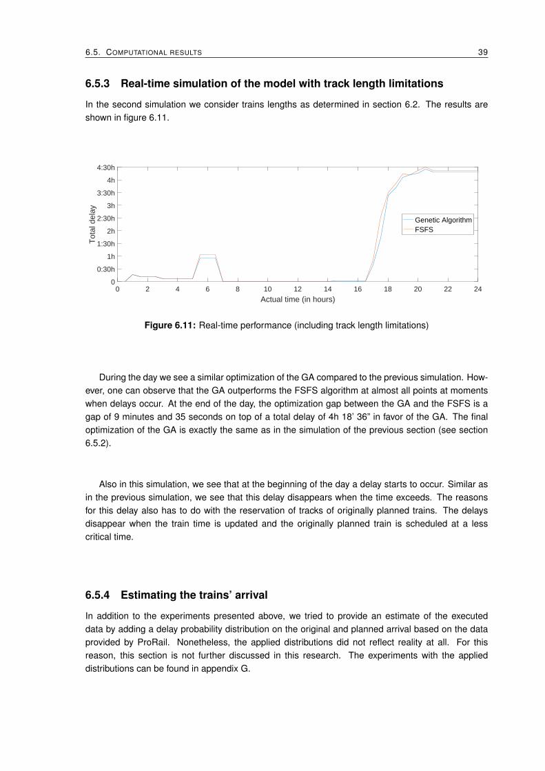
6.5. COMPUTATIONAL RESULTS 39
6.5.3 Real-time simulation of the model with track length limitations
In the second simulation we consider trains lengths as determined in section 6.2. The results areshown in figure 6.11.
0 2 4 6 8 10 12 14 16 18 20 22 24
Actual time (in hours)
0
0:30h
1h
1:30h
2h
2:30h
3h
3:30h
4h
4:30h
Tot
al d
elay
Genetic AlgorithmFSFS
Figure 6.11: Real-time performance (including track length limitations)
During the day we see a similar optimization of the GA compared to the previous simulation. How-ever, one can observe that the GA outperforms the FSFS algorithm at almost all points at momentswhen delays occur. At the end of the day, the optimization gap between the GA and the FSFS is agap of 9 minutes and 35 seconds on top of a total delay of 4h 18’ 36” in favor of the GA. The finaloptimization of the GA is exactly the same as in the simulation of the previous section (see section6.5.2).
Also in this simulation, we see that at the beginning of the day a delay starts to occur. Similar asin the previous simulation, we see that this delay disappears when the time exceeds. The reasonsfor this delay also has to do with the reservation of tracks of originally planned trains. The delaysdisappear when the train time is updated and the originally planned train is scheduled at a lesscritical time.
6.5.4 Estimating the trains’ arrival
In addition to the experiments presented above, we tried to provide an estimate of the executeddata by adding a delay probability distribution on the original and planned arrival based on the dataprovided by ProRail. Nonetheless, the applied distributions did not reflect reality at all. For thisreason, this section is not further discussed in this research. The experiments with the applieddistributions can be found in appendix G.
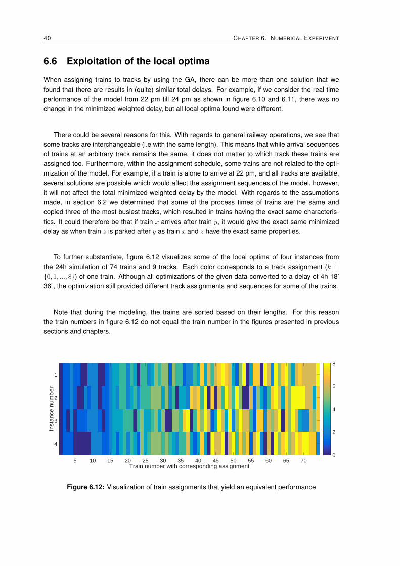
40 CHAPTER 6. NUMERICAL EXPERIMENT
6.6 Exploitation of the local optima
When assigning trains to tracks by using the GA, there can be more than one solution that wefound that there are results in (quite) similar total delays. For example, if we consider the real-timeperformance of the model from 22 pm till 24 pm as shown in figure 6.10 and 6.11, there was nochange in the minimized weighted delay, but all local optima found were different.
There could be several reasons for this. With regards to general railway operations, we see thatsome tracks are interchangeable (i.e with the same length). This means that while arrival sequencesof trains at an arbitrary track remains the same, it does not matter to which track these trains areassigned too. Furthermore, within the assignment schedule, some trains are not related to the opti-mization of the model. For example, if a train is alone to arrive at 22 pm, and all tracks are available,several solutions are possible which would affect the assignment sequences of the model, however,it will not affect the total minimized weighted delay by the model. With regards to the assumptionsmade, in section 6.2 we determined that some of the process times of trains are the same andcopied three of the most busiest tracks, which resulted in trains having the exact same characteris-tics. It could therefore be that if train x arrives after train y, it would give the exact same minimizeddelay as when train z is parked after y as train x and z have the exact same properties.
To further substantiate, figure 6.12 visualizes some of the local optima of four instances fromthe 24h simulation of 74 trains and 9 tracks. Each color corresponds to a track assignment (k =
{0, 1, ..., 8}) of one train. Although all optimizations of the given data converted to a delay of 4h 18’36”, the optimization still provided different track assignments and sequences for some of the trains.
Note that during the modeling, the trains are sorted based on their lengths. For this reasonthe train numbers in figure 6.12 do not equal the train number in the figures presented in previoussections and chapters.
5 10 15 20 25 30 35 40 45 50 55 60 65 70Train number with corresponding assignment
1
2
3
4
Inst
ance
num
ber
0
2
4
6
8
Figure 6.12: Visualization of train assignments that yield an equivalent performance

Chapter 7
Discussion
In chapter 3 we identified the Real-Time Track Assignment Problem (RT-TAP) as an assignmentproblem that resulted from deviations in the original schedule because of disruptions and last-minuterequests of train operators. In order to provide a solution for the RT-TAP, we developed the followingaim that stayed central in this research:
To develop a fast and easy usable Decision Support System (DSS) that, if delays occur, reassignsinbound trains to tracks in order to minimize the total weighted delays of outbound trains at anyrailway yard at real-time.
After formulating the model as a mixed integer program, we successfully developed a DSS thatreassigns inbound trains by minimizing the total weighted delays at a railway yard by using a BruteForce (BF) attack. Because of the computational complexity of the problem, a BF attack would notwork when considering larger instances. For this reason, we developed a problem specific GeneticAlgorithm (GA) that tries to find a ”reasonable good” solution based on natural selection and survivalof the fittest and a First Scheduled First Served (FSFS) heuristic for fast computation of solutions.
To validate the solutions methods, we first performed numerical experiments on a smaller instancein order to determine the optimality gap between the GA, FSFS, and the BF approach. To validatethe performance of the GA for an actual case including real-time changes in arrival times of trains, weexecuted the model in a 24h simulation based on historical data, provided by the Rail InfrastructureManager (RIM), of a Dutch railway yard named Waalhaven Zuid (Whz), and compared it with a FSFSheuristic approach.
When considering the smaller instances, we saw that when we don’t consider the train lengths,there is no significant difference between the computational performance of the three solution algo-rithms. However, when considering the variation of length of trains, we noticed that the GA performedup to 48% better than the FSFS algorithm in one of the instances. In another case, while the FSFSreduced the total delay to 6h 24’ 45”, the GA was able to minimize the same input to a total delay of4h 41’ 48”. In all instances, the GA equaled the solution provided by the BF approach.
When it comes to minimizing the total weighted delay for larger instances, the model providedoptimal solutions within 1,5 to 2 minutes of computation for a railway yard with 9 tracks and 74inbound trains. When comparing the GA with the FSFS algorithm, we showed that there was againno significant difference in delay when excluding the train length from the input. However, when weinclude different train lengths (i.e. not all trains can be parked at all tracks), we saw that the GAperformed slightly better than the FSFS assignment method, with a delay gap of 9 minutes and 35seconds on top of a total delay of 4h 18’ 36”. An important finding was that at the end of the real-time
41
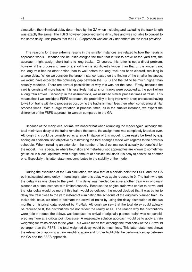
42 CHAPTER 7. DISCUSSION
simulation, the minimized delay determined by the GA when including and excluding the track lengthwas exactly the same. The FSFS however perceived some difficulties and was not able to convert tothe same delay. This proves that the FSFS approach was actually dependent on the input provided.
The reasons for these extreme results in the smaller instances are related to how the heuristicapproach works. Because the heuristic assigns the train that is first to arrive at the yard first, theapproach might assign short trains to long tracks. Of course, this latter is not a direct problem,however if the processing time of a short train is significantly longer than that of the longer train,the long train has no other option than to wait before the long track has been cleared, resulting ina large delay. When we consider the larger instance, based on the finding of the smaller instances,we would have expected the optimality gap between the FSFS and the GA to be much higher thanactually modeled. There are several possibilities of why this was not the case. Firstly, because theyard is consists of more tracks, it is less likely that all short tracks were occupied at the point whena long train arrives. Secondly, in the assumptions, we assumed similar process times of trains. Thismeans that if we consider a FSFS approach, the probability of long trains with short processes havingto wait on trains with long processes occupying the tracks is much less then when considering similarprocess times. With a large variation in process times, as in the smaller instance, we expect thedifference of the FSFS approach to worsen compared to the GA.
Because of the many local optima, we noticed that when rerunning the model again, although thetotal minimized delay of the trains remained the same, the assignment was completely knocked over.Although this could be considered as a large limitation of this model, it can easily be fixed by e.g.adding an additional soft objective by minimizing the total changes made with regards to the previousschedule. When including an extension, the number of local optima would actually be beneficial forthe model. This is because where heuristics and meta-heuristic approaches are known to sometimesget stuck in a local optimum, with a high amount of possible solutions it is easy to convert to anotherone. Especially this latter statement contributes to the stability of the model.
During the execution of the 24h simulation, we saw that at a certain point the FSFS and the GAboth calculated some delay. Interestingly, later this delay was again reduced to 0. The train who gotthe delay was one close to the yard. This delay was needed because another train was originallyplanned at a time instance with limited capacity. Because the original train was earlier to arrive, andthe total delay would be more if this train would be delayed, the model decided that it was better todelay the train close to the yard instead of eliminating the schedule of the originally planned train. Totackle this issue, we tried to estimate the arrival of trains by using the delay distribution of the twomonths of historical data received by ProRail. Although we saw that the total delay could actuallybe reduced to 0, the distributions did not reflect the reality at all. The reason why the distributionswere able to reduce the delays, was because the arrival of originally planned trains was not consid-ered anymore at a critical point because. A reasonable solution approach would be to apply a trainweighting for trains closer to the yard. This would mean that although the total delay of the GA wouldbe larger than the FSFS, the total weighted delay would be much less. This latter statement showsthe relevance of applying a train weighting again and further highlights the performance gap betweenthe GA and the FSFS approach.

43
Main contributions
To sum up the main contribution of this research:
• we provided new insights in the (computational) complexity of Real-Time track assignment;
• developed a mathematical program that is able to solve the RT-TAP;
• developed a problem specific GA that solves the RT-TAP within 1,5 to 2 minutes without, to bestof our knowledge, compromising the global optimum;
• created new insights into the relation between the complexity of the assignment and the inputof the model, which were not earlier discussed in the literature.
Limitations
Concerning the limitations to the approach:
• rail freight transportation has many uncertainties about the future. E.g. next to Whz was the RailService Center (RSC). If a train would finish its operations at RSC before or after scheduled, itwould need a immediate assignment at the yard. It is uncertain what the effects are with thismodel on the assignment when this would happen;
• the model successfully allocated trains to track. However, we found many local optima in thesolution space. While the minimized delays remained the same, the assignment was completelyknocked over every time when running the model again;
• we can apply large weightings when a train is parked, and therefore fix the delay of a train,however, because we were not able to fix tracks, the model can still reassign a train to anothertrack even if the train is already parked;
• we compared the GA with a FSFS approach. Although this latter approach is widely used inliterature, it is unknown how this approach reflects the actual real-time assignments of a TrainDispatcher (TD);
• because visiting an actually traffic control post was not possible, we could not compare theproposed method with an actual real-time assignment of a TD. It is therefore unknown how thismodel will improve the current assignment process;

44 CHAPTER 7. DISCUSSION
To sum up the main limitation with regards to the numerical experiment:
• the Numerical Experiment was only limited to the railway yard Whz. The performance of themodel at other railway yards is therefore unknown and could differ;
• the data provided by ProRail showed many gaps with regards to the data needed for the modelto perform. For example, the data did not include all lengths of all trains, did not show an arrivaltime of trains with a corresponding departure, and therefore we also assumed the processtimes of each train at the yard. Especially the assumption with regards to the process timesmay have improved the performance of the FSFS algorithm. As we saw from our own madescenario, when considering a large deviation in process times and l the gap between the GAand the FSFS algorithm is much higher than with similar processes;
• the numerical experiments are tested based on executed historical data. This means that thedata could give a distorted picture as the problems that occurred at real-time problems mightalready be solved in this data;
• we made many assumptions with regards to length, process times and arrival times of trainswhich where needed for the model to perform. If these assumptions are relaxed, the resultscould differ than presented in this thesis.
Future research directions
Concerning the limitation of the approach, future research direction may consider extending themodel with regards to the number of changes made in the schedule and be able to fix track as-signments of a train. This could be done for example adding soft constraints or by applying ’sectionoptimization’, where we only consider optimizing the part which includes a delayed train. Moreover,more detailed observations can be performed to better understand the task and decisions made bya TD, and show a better comparison between the model and the actual real-time track assignments.
When considering an actual implementation of the model, it is important to first have a betterinformation exchange so more accurate data is known. For example, the data of ProRail showeda high stochastic arrival of trains. Trains might just pop-up when finished with operations at RSC,which made it very difficult to get a stable assignment. It might therefore be interested to performresearch for an integrated approach for data exchange to gain better insights in when trains arrive,depart, have delays, etc.
We tried to make a better expectation of the arrival of trains by applying a delay distribution.Although this method did not reflect the reality at all, a stochastic optimization (i.e. Monte Carlo),could be tried to make a better approximation of the arrivals of trains. Furthermore, to increase therobustness of the assignment, it might be an idea to incorporate an buffer of trains as a soft constraintto the mathematical model.
With regards to additional application of the model, because of the fast and accurate performance,similar as discussed by Gilg et al. (2018), we see the possibility to enhance the proposed modelfor the task of designing railway yards, assessing the effects of putting tracks out of service formaintenance, or for a sensitivity analysis of bottlenecks on railway yards in the overall network.
When considering improving the performance of the solution method (i.e. of the GA), we sawthat the solutions provided by the FSFS algorithm were already generally good solutions. As vanHove (2019) also suggested in her thesis, running the model with a warm start, i.e. starting with aninitial solution generated by a quick method, could contribute to the computational performance andstability of the assignments of the model.

Chapter 8
Conclusion
The thesis at hand aimed in creating a Decision Support System (DSS) that assists a Train Dispatcher(TD) in finding optimal track assignments for each inbound train by minimizing the total weighted delayat any railway yard. Real-Time assignment problems resulting from large stochastic arrival of freighttrains is formulated as the Real-Time Track Assignment Problem (RT-TAP). We presented the modelas a mixed integer program and proved the general case to be NP-hard because of its strong relationwith the Vehicle Routing Problem (VRP). By reason of the computational complexity of the problem, aBrute Force (BF) approach would not work to solve the RT-TAP when considering larger instances atreal-time. Therefore, a problem specific Genetic Algorithm (GA) was employed for finding ’reasonablegood’ solutions to the problem. After the execution of several tests, results showed that there is nooptimality gap between the performance of the BF method and the GA for smaller instances.
Application of the model shows that when excluding the lengths from the input, the results indicatea small optimality gap between the overall performance of the GA and the First Scheduled FirstServed (FSFS) approach for both smaller and larger instances in favor of the GA. When consideringtrack limitations of trains (i.e. not all trains can be parked at all tracks), the results showed for smallerinstances that the GA performed up to 48% better than the FSFS. Better performance of the GA alsoaccounted on the larger instances as the FSFS was not able to provide solutions as good as the GA.
To conclude, the obtained results demonstrated that while the GA gave a stable performance,the performance of the FSFS approach was strongly related with the input, such as the length andarrival times of the trains. This latter showed that there is a relation between the complexity of theproblem and the input that is provided. The use of this DSS can therefore not only stabilize, butalso improve current decisions making with regards to real-time track assignment, and should beconsidered especially before e.g. investing in additional infrastructure at railway yards.
45

46 CHAPTER 8. CONCLUSION

Bibliography
Bettinelli, A., Santini, A., and Vigo, D. (2017). A real-time conflict solution algorithm for the train reschedulingproblem. Transportation Research part B, vol 106:237–265.
Boysen, N., Fiedner, M., Jaehn, F., and Pesch, E. (2012). Shunting yard operations: Theoretical aspects andapplications. European Journal of Operational Research, vol 220(1):1–14.
Briggs, N. and Beck, C. (2007). Modeling train delays with q-exponential functions. Physica A: StatisticalMechanics and its Applications, vol 378(2):498–504.
Cacchiani, V., Huisman, D., Kidd, M., Kroon, L., Toth, P., Veelenturf, L., and Wagenaar, J. (2014). An overviewof recovery models and algorithms for real-time railway rescheduling. Transportation Research Part B, vol63:15–37.
Cai, X. and Goh, C. (1994). A fast heuristic for the train scheduling problem. Computers & Operations Research,vol 21(5):499–510.
Corman, F., D’Ariano, A., Pacciarelli, D., and Pranzo, M. (2010). A tabu search algorithm for rerouting trainsduring rail operations. Transportation Research Part B, vol 44:175–192.
D’Ariano, A. (2015). Improving real-time train dispatching: Models, algorithms and applica-tions. [PhD Thesis] https://www.google.com/url?sa=t&rct=j&q=&esrc=s&source=web&cd=2&ved=
2ahUKEwjhr4e-3JviAhUSDuwKHTImBHIQFjABegQIAhAC&url=https%3A%2F%2Frepository.tudelft.nl%
2Fislandora%2Fobject%2Fuuid%3A178b886e-d6c8-4d39-be5d-03d9fa3a680f%2Fdatastream%2FOBJ%
2Fdownload&usg=AOvVaw3PKpXVxJTtJ-NtvKMWgkWx. Accessed on 14 May 2019.
Dollevoet, T. and Huisman, D. (2014). Fast heuristics for delay management with passenger rerouting. PublicTransport, 6(1):67–84.
Dollevoet, T., Huisman, D., Kroon, L. G., Veelenturf, L. P., and Wagenaar, J. C. (2010). Application of an iterativeframework for real-time railway rescheduling. Computers Operations Research, vol 78:203–217.
Dollevoet, T., Schmidt, M., and Schobel, A. (2011). Delay management including capacities of stations. InATMOS.
European Commission (2014). Fourth report on monitoring development of the rail market. [PDF]https://eur-lex.europa.eu/resource.html?uri=cellar:d261b1f8-f5f4-11e3-831f-01aa75ed71a1.
0002.01/DOC_2&format=PDF. Accessed on 14 May 2019.
Fang, W. (2015). A survey on problem models and solution approaches to rescheduling in railway networks.IEEE Transactions on Intelligent Transportation Systems, vol 16(6):2997–3016.
Fischettia, M. and Monaci, M. (2017). Using a general-purpose mixed-integer linear programming solver for thepractical solution of real-time train rescheduling. European Journal of Operational Research, vol 263:258–264.
Gatto, M., Maue, J., Mihalak, M., and Widmayer, P. (2009). Shunting for dummies: an introductory algorithmicsurvey. Springer.
47

48 BIBLIOGRAPHY
Gestrelius, S., Aronsson, M., Joborn, M., and Bohlin, M. (2017). Towards a comprehensive model for trackallocation and rolltime scheduling at marshalling yards. Journal of Rail Transport Planning Management, vol7:157–170.
Gilg, B., Klug, T., Martienssen, R., Paat, J., Schlechte, T., Schulz, C., Seymen, S., and Tesch, A. (2018). Conflict-free railway track assignment at depots. Rail Transport Planning & Management, vol 8:16–28.
Givoni, M. and Banister, D. (2013). Moving Towards Low Carbon Mobility. Edward Elgar.
Gkiotsalitis, K., Wu, Z., and Cats, O. (2019). A cost-minimization model for bus fleet allocation featuring thetactical generation of short-turning and interlining options. Transportation research. Part C: Emerging tech-nologies, vol 98:14–36.
Glover, F. (1986). Future paths for integer programming and links to artificial intelligence. Computers & Opera-tions Research, vol 13(5):533–549.
Haahr, J. and Lusby, R. (2017). Integrating rolling stock scheduling with train unit. European Journal of Opera-tional Research, vol 259(2):452–468.
Haahr, J., Lusby, R., and Wagenaar, J. (2017). Optimization methods for the train unit shunting problem. Euro-pean Journal of Operational Research, vol 262(3):981–995.
Hansmann, R. S. and Zimmermann, U. T. (2008). Optimal Sorting of Rolling Stock at Hump Yards, pages189–203. Springer Berlin Heidelberg, Berlin, Heidelberg.
Ho, T. and Yeung, T. (2001). Railway junction traffic control by heuristic methods. Electric Power Applications,IEE Proceedings, 148:77–84.
Hoenders, C. (2018). Interview with Cor Hoenders from Rail Cargo, 6 november 2018.
Holland, J. (1975). Adaptation in natural and artificial systems. University of Michigan Press, Michigan.
Jaehn, F., Otto, A., and Seifried, K. (2018). Shunting operations at flat yards: retrieving freight railcars fromstorage tracks. OR Spectrum, vol 40(2):367–393.
Jaehn, F., Rieder, J., and Wiehl, A. (2015). Single-stage shunting minimizing weighted departure times. Omega,vol 52:133–141.
Josyula, S. P., Krasemann, J. T., and Lundberg, L. (2018). A parallel algorithm for train rescheduling. Trans-portation Research Part C, vol 95:545–569.
Karp, R. M. (1972). Reducibility among combinatorial problems. Complexity of Computer Computations, pages85–103.
Keyrail (2014). Process reports of trains at Waalhaven Zuid. [report].
Liong, C.-Y., Wan, I., and Omar, K. (2008). Vehicle routing problem: Models and solutions. Journal of QualityMeasurement and Analysis, vol 4:205–218.
Narayanaswami, S. and Rangaraj, N. (2011). Scheduling and rescheduling of railway operations: A review andexpository analysis. Technology Operation Management, vol 2(2):102–122.
Network Rail (2016). Value and importance of rail freight. [PDF] http://www.networkrail.co.uk/wp-content/uploads/2016/11/The-Value-and-Importance-of-rail-Freight-summary-report.pdf. Accessed on 07February 2019.
Pachl, J. (2004). Railway operations and Control. Vtd Rail Pub.
Pferschy, U. and Stanek, R. (2017). Generating subtour elimination constraints for the TSP from pure integersolutions. Central European Journal of Operations Research, vol 25(1):231–260.

BIBLIOGRAPHY 49
Pinedo, M. L. (2016). Scheduling: Theory, Algorithms, and Systems. Springer, Cham.
Piner, D. and Condry, D. (2017). International best practices in managing unplanned disruption to suburban railservices. Transportation Research Procedia, vol 25:4403–4410.
ProRail (2015). Two months of historical data about train arrivals and departures at Waalhaven Zuid.
Rahim, S. K. N. A., Bargiela, A., and Qu, R. (2013). Hill climbing versus genetic algorithm optimization insolving the examination timetabling problem. Proceedings of the 2nd International Conference on OperationsResearch and Enterprise Systems, vol 1:43–52.
Roland Rail (2015). Dienstregeling goederentreinen from Roland Rail schedule database. [Report].
Schachtebeck, M. and Schobel, A. (2008). Ip-based techniques for delay management with priority decisions.In ATMOS.
Schachtebeck, M. and Schobel, A. (2010). To wait or not to wait and who goes first? Delay management withpriority decisions. Transportation Science, vol 44(3):307–321.
Schobel, A. (2007). Integer Programming Approaches for Solving the Delay Management Problem. Springer,Berlin, Heidelberg. In: Geraets F., Kroon L., Schoebel A., Wagner D., Zaroliagis C.D. (eds) AlgorithmicMethods for Railway Optimization. Lecture Notes in Computer Science, vol 4359.
Schobel, A. (2009). Capacity constraints in delay management. Public Transport, vol 1(2):135–154.
Spoorcafe (2018). Network gathering with several rail freight transportation companies, 29 november 2018.
Sporenplan (2016). Drawings of Waalhaven Zuid. [drawings] www.sporenplan.nl. Accessed on 27 January2019.
Timmermans, P. (2018). Interview with Patrick Timmermans from ProRail, 12 october 2018.
Tornquist, J. (2010). Greedy algorithm for railway traffic re-scheduling during disturbances: A swedish case. IETIntelligent Transport Systems, vol 4(4):75–386.
Tornquist, J. (2012). Design of an effective algorithm for fast response to the re-scheduling of railway trafficduring disturbances. Transportation research. Part C: Emerging technologies, vol 20(1):62–78.
Tornquist, J. and Persson, J. A. (2005). Train traffic deviation handling using tabu search and simulated anneal-ing. Proceedings of the 38th Annual Hawaii International Conference on System Sciences, pages 73a–73a.
U.S. Department of Transportation (1999). Understanding how train dispatchers manage and control trains: Acognitive task analysis of a distributed team planning task. [PDF] http://citeseerx.ist.psu.edu/viewdoc/download?doi=10.1.1.876.1554&rep=rep1&type=pdf. Accessed on 14 May 2019.
U.S. Railroad (2008). A review of capacity and performance data. [online] . Accessed on 07 January 2019.
van Hove, E. (2019). Train routing at the shunt yard : a disjoint paths approach. [Master Thesis] http://essay.utwente.nl/77267/. Accessed on 08 May 2019.
Winter, T. and Zimmermann, U. (2000). Real-time dispatch of trams in storage yards. Annals of OperationalResearch, vol 96:287–315.
Zhan, S., Kroon, L. G., Veelenturf, L. P., and Wagenaar, J. C. (2015). Real-time high-speed train rescheduling incase of a complete blockage. Transportation Research Part B, vol 78:182–201.

50 BIBLIOGRAPHY

Appendix A
MOD file of the AMPL model
The following shows the .MOD file necessary for running the AMPL model. The model is based onthe mathematical formulation described in chapter 4.
reset;
#sets
set N ordered;
set K;
set z_b;
set z_e;
#input for trains
param arrival_n {i in N};
param departure_n {i in N};
param length_n {i in N};
param weighting_n {i in N};
param beta; #followup time of trains
var process {i in N};
#input for tracks
param length_k {k in K};
#other parameters
param C;
param g := card(N);
#defining the subtour elimination
set S := 0 .. (2**g-1);
set POW {s in S} := {n in N: (s div 2**(ord(n,N)-1)) mod 2 == 1};
#binary varibales, assigned or not
var x {i in N , j in N, k in K} binary;
var y {q in z_b , i in N, k in K} binary;
var z {i in N , p in z_e, k in K} binary;
#new determined
var aks_arrival_n {i in N, k in K};
var aks_departure_n {i in N, k in K};
var tilde_arrival_n {i in N};
51

52 APPENDIX A. MOD FILE OF THE AMPL MODEL
var tilde_departure_n {i in N};
#result
var differ {i in N};
var W_differ {i in N};
### SEQUENCE ###
subject to seq1 {i in N}:
sum {k in K} (sum {j in N} x[i,j,k] + sum {p in z_e} z[i,p,k]) = 1;
subject to seq2 {j in N}:
sum {k in K} (sum {i in N} x[i,j,k] + sum {q in z_b} y[q,j,k]) = 1;
subject to seq3 {k in K, q in z_b}:
sum {i in N} y[q,i,k] <= 1;
subject to seq4 {k in K, p in z_e}:
sum {i in N} z[i,p,k] <= 1;
subject to seq5 {i in N, k in K}:
(sum {j in N} x[j,i,k] + sum {q in z_b} y[q,i,k]) - (sum {j in N} x[i,j,k] + sum {p in z_e} z[i,p,k]) = 0;
subject to SUBS {s in S: card(POW[s]) >= 1}:
sum {i in POW[s], j in POW[s], k in K} x[i,j,k] <= card(POW[s]) - 1;
### TIME ###
subject to time1 {i in N, j in N, k in K}:
aks_departure_n[i,k] - C*(1 - x[i,j,k]) + beta <= aks_arrival_n[j,k];
subject to time2 {i in N, k in K}:
aks_arrival_n[i,k] >= arrival_n[i];
subject to time3 {i in N, k in K}:
tilde_arrival_n[i] >= aks_arrival_n[i,k];
subject to time4 {i in N, k in K}:
aks_departure_n[i,k] = aks_arrival_n[i,k] + process[i];
subject to time5 {i in N}:
tilde_departure_n[i] = tilde_arrival_n[i] + process[i];
subject to ProcessTime {i in N}:
departure_n[i] - arrival_n[i] = process[i];
### LENGTH ###
subject to len1 {i in N, j in N, k in K: length_n[i] > length_k[k]}:
x[i,j,k] = 0;
subject to len2 {q in z_b, i in N, k in K: length_n[i] > length_k[k]}:
y[q,i,k] = 0;
subject to len3 {i in N, p in z_e, k in K: length_n[i] > length_k[k]}:
z[i,p,k] = 0;
### RESULT ###
subject to result {i in N}:
differ[i] = tilde_departure_n[i] - departure_n[i];
subject to Weigthed_result {i in N}:
W_differ[i] = ((tilde_departure_n[i] - departure_n[i]) * weighting_n[i]);
### MINIMIZED FUNCTION ###
minimize f:
sum {i in N} ((tilde_departure_n[i] - departure_n[i]) * weighting_n[i]);

Appendix B
DATA file of the AMPL model
The following shows an example of a .DATA file necessary for the AMPL model to run.
### SCENARIO 2 ###
set N := train1 train2 train3 train4 train5 train6 train7 train8 train9 train10 train11 train12 train13;
set K := track1 track2 track3 track4;
set z_b:= Begin;
set z_e:= End;
param C := 10000000; ### DO NOT CHANGE ###
param beta := 300; #follow up time of trains is: 300 seconds = 5 min
### INPUT TRACKS ###
param length_k :=
track1 350
track2 500
track3 200
track4 800
;
### INPUT TRAINS ###
param arrival_n :=
train1 15300
train2 29700
train3 29700
train4 30900
train5 28900
train6 33900
train7 41100
train8 35940
train9 45540
train10 46800
train11 36000
train12 53700
train13 57780
;
param departure_n :=
53

54 APPENDIX B. DATA FILE OF THE AMPL MODEL
train1 26040
train2 35400
train3 35400
train4 36600
train5 75000
train6 37800
train7 46800
train8 44040
train9 53640
train10 52500
train11 49200
train12 59400
train13 65880
;
param length_n:=
train1 750
train2 200
train3 750
train4 400
train5 350
train6 600
train7 800
train8 200
train9 100
train10 50
train11 600
train12 300
train13 650
;
param weighting_n:=
train1 1
train2 1
train3 1
train4 1
train5 1
train6 1
train7 1
train8 1
train9 1
train10 1
train11 1
train12 1
train13 1
;

Appendix C
RUN file of the AMPL model
The following shows the .RUN file of the AMPL model.
reset;
model ’/Users/bramschasfoort/Desktop/amplide/Thesis/RTTAP.mod’;
data ’/Users/bramschasfoort/Desktop/amplide/Thesis/RTTAP.dat’;
option solver cplex;
solve;
display x;
display y;
display z;
display arrival_n;
display tilde_arrival_n;
display departure_n;
display tilde_departure_n;
display differ;
#display W_differ;
#display length_n;
#display length_k;
display _total_solve_time;
55

56 APPENDIX C. RUN FILE OF THE AMPL MODEL
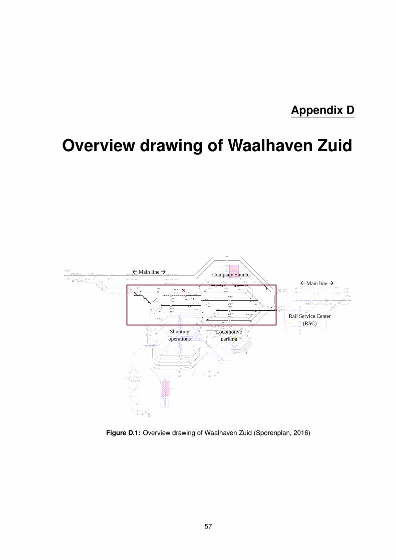
Appendix D
Overview drawing of Waalhaven Zuid
Master Thesis – Bram Schasfoort – Concept 22.05.2019 72
Appendix 9: Total overview drawing of Waalhaven-zuid.
Figure X. 4: Total overview drawing of Waalhaven-zuid (sporenplan.nl, 2016).
Rail Service Center
(RSC)
Company Shunter
Shunting
operations
Locomotive
parking
Main line
Main line
Figure D.1: Overview drawing of Waalhaven Zuid (Sporenplan, 2016)
57

58 APPENDIX D. OVERVIEW DRAWING OF WAALHAVEN ZUID

Appendix E
Determining process times of trains
Problems in the received data from ProRail is that the data did not show an arrival time with its correspondingdeparture time. The data received consisted of a list of train number including if the train is ether arriving,departing or driving though the yard, and the times as discussed in previous section. This seemed like aproblem however, all trains operating on the network in the Netherlands are linked with a train number.
The train number is linked with its origin and destination and with the road travelled by a train (see figureE.1). If for example a train departs from A and arrives at B, it could receive an even train number 40000. If thesame train would again depart from B in the direction of A, it will receive an uneven train number in the samesequence (for example 40001). With this knowledge, a train departing from B in the direction of destination C,could never receive a train number in the sequence of 40000, but will get a number of for example 40300. Thesame train then departing again from C in the direction of B would then receive the number 40301. Important toknow is that all train numbers will be reset at midnight.
Master Thesis – Bram Schasfoort – Concept 22.05.2019 40
Train number setup and operations.
Problems in the received data from ProRail is that the data did not show an arrival time with its
corresponding departure time. The data received consisted of a list of train number including if the
train is ether arriving, departing or driving though the yard, and the times as discussed in previous
chapter. However, all trains performing on the network in the Netherlands are linked with a train
number. The train number is linked with its origin and destination (see figure 8.2). Furthermore,
the following train number sequences are linked with the road travelled by a train. If for example a
train departs from A and arrives at B, it could receive an uneven train number 40001. If the same
train would again depart from B in the direction of A, it will receive an even train number in the
same sequence (for example 40002). For this reason, a train departing from B in the direction of
destination C, could never receive a train number in the sequence of 40000, but will get a number
for example 40300. Important to know is that all train numbers will be reset at midnight.
Knowing the train number setup, the trains in the list with the same train number on the same day
could be linked with each other, and numbers in a sequential train number can by strongly assumed
that they have a destination at Whz. To further conform the data, the year plan many train including
train numbers, origin, destination and in-between stops were also provided by RolandRail (2015),
and therefore could be double checked with the data received from ProRail.
The trains arriving and departing from the yard can be divided in two dif ferent categories.
1. Trains passing through Whz.
2. Trains with origin or destination Whz (RSC).
With the above knowledge, trains arriving and departing with the same train numbers on the same
day could be linked which gave a train’s arrival and corresponding departure time. Furthermore,
this gives also the time a train remained at the yard.
The problem with the other category is that because the origin or destination is Whz, it could not
be determined from the data provided how long a train had to remain at the yard, or more specific,
a track.
The data provided by ProRail did not show the arrival and corresponding
departure time of a train.
Figure 8.2: Train number setup of the Dutch railway network.
A B C
Even train numbers
Uneven train numbers
Even train numbers
Uneven train numbers
Figure E.1: Train number setup of the Dutch railway network
By knowing the train number setup, we could link the trains in the list with the same train number on thesame day. Train numbers that had a number arriving and the same number departing at the same day canbe assumed that the train was driving through the yard and for example needed to wait for a path. The trainswith a number when arriving and a number in the same sequence when departing where assumed to have adestination at Waalhaven Zuid (Whz) and therefore Rail Service Center (RSC). To further conform the data,many trains with data from the year plan including train numbers, origin, destination and in-between stops werealso provided by Roland Rail (2015), and could therefore be double checked with the data received from ProRail.The trains arriving and departing from the yard can therefore be divided in two different categories.
1. Trains passing through Whz.2. Trains with origin or destination Whz (RSC).
With the above knowledge, trains arriving and departing with the same train numbers on the same day couldbe linked with each other and gave a trains’ arrival and corresponding departure time which then also gives thetime a train remained at the yard. The problem with the other category is that because the origin or destinationis Whz, it could not be determined from the data provided how long a train had to remain at the yard, or morespecific, a track.
59

60 APPENDIX E. DETERMINING PROCESS TIMES OF TRAINS
Process times at Waalhaven Zuid
Because from the received data from ProRail could not be determined how long a train from the second categorywas occupying the track, additional data regarding the processes at the railway yard was required. According todocumentation from Keyrail (2014), trains from the second category must go through some operations. Whenarriving at Whz from the network, the process described in table E.1 should be used. When the train arrives atWhz from RSC and is prepared for the network, table E.2 is applied.
Table E.1: Processes when arriving at Waalhaven Zuid from the network and departing to Rail Ser-vice Center
Step Time of Operations Time needed1. Block train arrives at track k = {1, 2, ...,K} (incl. electrical locomotive) 5 min2. Electrical locomotive is detached and parked 15 min3. Train receives arrival check 30 min4. Optional buffer 0 min5. Diesel locomotive is attached (ether front of back of the train) 20 min6. Train pushed or pulled to RSC 20 min7. Locomotive is detached. Parking diesel locomotive 5 min
Total time needed at the yard after arriving at Whz : 95 min
Table E.2: Processes when departing from Waalhaven Zuid after visiting Rail Service CenterStep Time of Operations Time needed
1. Diesel locomotive is moved to RSC and attached to the train 10 min2. Block train moved to track k = {1, 2, ...,K} (incl. diesel loc). 20 min3. Diesel locomotive is detached and parked 20 min4. Electrical locomotive is attached 25 min5. Large break test 45 min6. Waiting for network path to be cleared 10 min7. Departure from Whz 5 min
Total time needed at the yard before departing from Whz : 135 min
Considering the above, the following process times are assumed:- Trains arriving at Whz have a process operation time of 1 hour and 35 min.- Trains departing from Whz have a process operation time of 2 hours and 15 min.
Including the arrival time of the trains and the process times determined above, we determined the followingoriginal train schedule:
123456789
101112
123456789
19 20 2138 44
8Track
nr.Original assignment schedule9 10 11 12 13 14 15 22 23
7 12 9 14 210 1 2 3 4 5 6 7
3223 26 3616 17 18
512 6 8 13 19 24 25 28 33 39 47
4 10 15 20 27
4130
No assignmentsNo assignments
17 22 34 3529 40 50
No assignmentsNo assignments
42 4818 31
37 43
Track nr.
Adjusted original assignment schedule9 10 11 12 2313 14 15 16 17 18 19 20 21
4
5139
7 12 9 14 442 6 8 13 19 24 25 28 33
21 23220 1 2 3 4 5 6 7 8
26 36 32 38
5017 22 34 35 42 48
47
18 31
10 15 20 27 29 40
32c 38c37 43
44c 51c2c 6c 8c 13c 19c 24c
7c 12c 9c 14c 21c 23c 26c 36c
29c 40c 50c25c 28c 33c 39c 47c
4c 10c 15c 20c 27c
Figure E.2: Visualization of the original train scheduled

Appendix F
Generating Length
The track assignment and the length of the trains was received in the same document. However, the problemsconsidering the data was that it was incomplete. In the overview only a small percentage of the lengths andexecuted track assignments were shown. Because the data might miss the normative lengths, the receivedlengths of trains are not considered in the model. Because ProRail was not able to provide the train lengths wegenerate a random length for each train.
Constructing the train length for each train is done as follows:Begin function
For every i ∈ N : Generate random number from 0 to 100%
If random nr. > 95% : li = 740 meterElse if random nr. > 80% : li = random nr. between (620− 700) meterElse if random nr. > 50%: li = random nr. between (550− 600) meterElse li = 400 meter
End function
The only condition with regards to the length was that if we execute the model based on original data, thetotal delay has to be 0 seconds. This is because also in practice no schedule will be made in the beginning ofthe day which starts with a delay.
61

62 APPENDIX F. GENERATING LENGTH

Appendix G
Delay distribution of trains
We saw that the optimization of the total delays is highly dependent on the original and planned schedule ofother trains. For example, we saw that because a train was delayed we reduced the expected total delay from55 minutes and 58 seconds at 6 am, to a 0 minute delay at 10 am. The main reason for applying a stochasticoptimization is to see what happens to the total weighted delay when including different distributions on thearrival times of trains.
The stochastic optimization is done at two different moments on both scenarios where we consider the tracklimitations and at two different moments where we do not consider the lengths. In the stochastic model wecompute solutions based on the trains expected delays with four different probability ranges (50%, 30% to 70%,10% to 90%, 5% to 95%). Each probability rage is computed five times.
Based on the data received from ProRail, we determined the following mean values and standard deviations(See table G.1).
Table G.1: Trains’ delay, mean values and variancesMean value Standard deviation Sample size
Original to executed (arrival) 00 : 50 : 35 02 : 19 : 03 260
Planned to executed (arrival) 00 : 01 : 18 00 : 19 : 07 289
Figure G.1 and G.2 visualize the distributions and the histograms of the delays on the trains’ arrivals fromthe original data compared with the executed data, and the planned data compared with the executed datarespectively.
63

64 APPENDIX G. DELAY DISTRIBUTION OF TRAINS
-6 -5 -4 -3 -2 -1 0 1 2 3 4 5 6 7 8 9 10 11 12
Hours of delay
0
25
50
75
100
125
150
Num
ber
of tr
ains
Figure G.1: Delay distribution on arrivals of trains (original compared with executed data)
-1 -0.9 -0.8 -0.7 -0.6 -0.5 -0.4 -0.3 -0.2 -0.1 0 0.1 0.2 0.3 0.4 0.5 0.6 0.7 0.8 0.9 1Hours of delay
0
50
100
150
200
250
Num
ber
of tr
ains
Figure G.2: Delay distribution on arrivals of trains (planned compared with executed data)
Results of stochastic optimization
Including the distributions determined above, we executed the model five different times for each different rangeat two different times on the two different scenarios.
During different tests we saw that at 46 am the model even optimized to a 0 second delay when the distri-butions were applied. On average, we see that the 50% distribution performs best for all scenarios. Figure G.3shows the results when adding the different distributions on arrival times at two time instances for the scenariowhere the train length is not considered. From this figure one can observe that the total range of delays lays onaverage between 1h 17’ 59” when including a distribution range of 10% to 90%, and a 0h 22’ 33” delay whenusing the 40% distribution for the time instance of 6 am. At the time instance of 10 am, one can observe that thetotal range of delays lays on average between 0h 43’ 24” when including a 90% distribution, and that the delayconverges to 0 seconds when excluding the distributions. Important to note is that the distribution ranges of 30%to 70%, 10% to 90%, and 5% to 95%, all have at least one result where the total weighted delay converged to 0
seconds.

65
0 80 160 240 320 400 480
Populations created (x102)
0h
0:15h
0:30h
0:45h
1h
1:15h
1:30h
1:45hT
otal
del
ay
0 80 160 240 320 400 480
Populations created (x102)
0h
0:15h
0:30h
0:45h
1h
1:15h
1:30h
1:45h
Tot
al d
elay
FSFS optimizationNo distributionDistribution with 50%Distribution with 70%Distribution with 90%Distribution with 95%
Figure G.3: Stochastic optimization excluding the length of trains for 6 am (left) and 10 am (right)
Figure G.4 visualizes the optimizations when we include the length of the trains for time instance 6 am and10 am. From this figure one can observe that at 6 am the Genetic Algorithm (GA) performed slightly betterthan the First Scheduled First Served (FSFS) scenario. When adding the distributions we can conclude that onaverage all tests perform better than the FSFS algorithm. When applying a distribution of 50%, the total weighteddelay again converges to 0h 22’ 33” delay. At 10 am we see that because we apply distributions on arrival oforiginal data delays occur further in the schedule.
0 80 160 240 320 400 480
Populations created (x102)
0h
0:15h
0:30h
0:45h
1h
1:15h
1:30h
1:45h
Tot
al d
elay
0 80 160 240 320 400 480
Populations created (x102)
0h
0:15h
0:30h
0:45h
1h
1:15h
1:30h
1:45h
Tot
al d
elay
Distribution with 95%FSFS optimizationNo distributionDistribution with 50%Distribution with 70%Distribution with 90%
Figure G.4: Stochastic optimization including the length of trains for 6 am (left) and 10 am (right)
On average the 50% distribution performs best in all four scenarios. Reason for the reduction could bethat in both cases the calculated delays at 6 am is based on the delay on trains that cannot be assignedbecause executed trains are parked at that point. The original place was reserved but the train was eventuallynot assigned there. If we include the distributions, we shift the original planned train that had trouble withassignment at 6 am, to an other moment where their assignment becomes less relevant. Hence, the total delayscan be further optimized, even to a point where they receive a 0 second delay for some of the instances.
Another important finding is that the solutions provided by the model when including a stochastic optimizationhave no relation with the executed data of the model. Because the delay of each train is very specific thedistribution do not give a valid estimation on which train does get the actual delay when the model is performed.For this reason the delays of trains determined by the model should always be decided as late as possible.