A decision support system for operations in a …murty/DSSpaper.pdfA decision support system for...
24
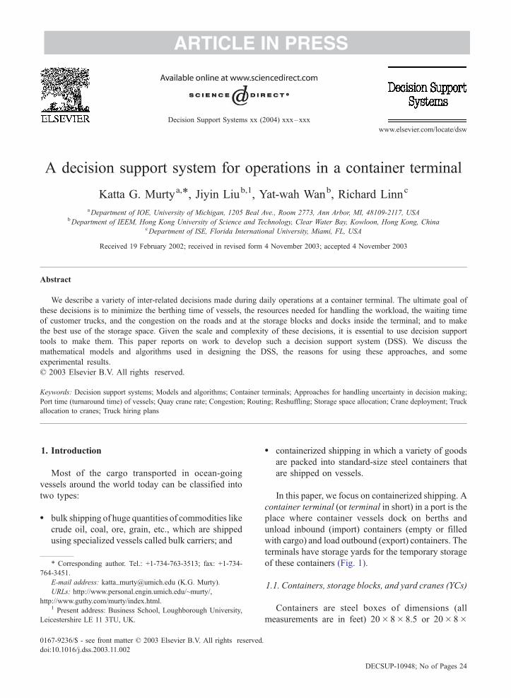
ARTICLE IN PRESS A decision support system for operations in a container terminal Katta G. Murty a, * , Jiyin Liu b,1 , Yat-wah Wan b , Richard Linn c a Department of IOE, University of Michigan, 1205 Beal Ave., Room 2773, Ann Arbor, MI, 48109-2117, USA b Department of IEEM, Hong Kong University of Science and Technology, Clear Water Bay, Kowloon, Hong Kong, China c Department of ISE, Florida International University, Miami, FL, USA Received 19 February 2002; received in revised form 4 November 2003; accepted 4 November 2003 Abstract We describe a variety of inter-related decisions made during daily operations at a container terminal. The ultimate goal of these decisions is to minimize the berthing time of vessels, the resources needed for handling the workload, the waiting time of customer trucks, and the congestion on the roads and at the storage blocks and docks inside the terminal; and to make the best use of the storage space. Given the scale and complexity of these decisions, it is essential to use decision support tools to make them. This paper reports on work to develop such a decision support system (DSS). We discuss the mathematical models and algorithms used in designing the DSS, the reasons for using these approaches, and some experimental results. D 2003 Elsevier B.V. All rights reserved. Keywords: Decision support systems; Models and algorithms; Container terminals; Approaches for handling uncertainty in decision making; Port time (turnaround time) of vessels; Quay crane rate; Congestion; Routing; Reshuffling; Storage space allocation; Crane deployment; Truck allocation to cranes; Truck hiring plans 1. Introduction Most of the cargo transported in ocean-going vessels around the world today can be classified into two types: bulk shipping of huge quantities of commodities like crude oil, coal, ore, grain, etc., which are shipped using specialized vessels called bulk carriers; and containerized shipping in which a variety of goods are packed into standard-size steel containers that are shipped on vessels. In this paper, we focus on containerized shipping. A container terminal (or terminal in short) in a port is the place where container vessels dock on berths and unload inbound (import) containers (empty or filled with cargo) and load outbound (export) containers. The terminals have storage yards for the temporary storage of these containers (Fig. 1). 1.1. Containers, storage blocks, and yard cranes (YCs) Containers are steel boxes of dimensions (all measurements are in feet) 20 8 8.5 or 20 8 0167-9236/$ - see front matter D 2003 Elsevier B.V. All rights reserved. doi:10.1016/j.dss.2003.11.002 * Corresponding author. Tel.: +1-734-763-3513; fax: +1-734- 764-3451. E-mail address: katta _ [email protected] (K.G. Murty). URLs: http://www.personal.engin.umich.edu/~murty/, http://www.guthy.com/murty/index.html. 1 Present address: Business School, Loughborough University, Leicestershire LE 11 3TU, UK. www.elsevier.com/locate/dsw DECSUP-10948; No of Pages 24 Decision Support Systems xx (2004) xxx – xxx
Transcript of A decision support system for operations in a …murty/DSSpaper.pdfA decision support system for...
ARTICLE IN PRESS
www.elsevier.com/locate/dsw
Decision Support Systems xx (2004) xxx–xxx
A decision support system for operations in a container terminal
Katta G. Murtya,*, Jiyin Liub,1, Yat-wah Wanb, Richard Linnc
aDepartment of IOE, University of Michigan, 1205 Beal Ave., Room 2773, Ann Arbor, MI, 48109-2117, USAbDepartment of IEEM, Hong Kong University of Science and Technology, Clear Water Bay, Kowloon, Hong Kong, China
cDepartment of ISE, Florida International University, Miami, FL, USA
Received 19 February 2002; received in revised form 4 November 2003; accepted 4 November 2003
Abstract
We describe a variety of inter-related decisions made during daily operations at a container terminal. The ultimate goal of
these decisions is to minimize the berthing time of vessels, the resources needed for handling the workload, the waiting time
of customer trucks, and the congestion on the roads and at the storage blocks and docks inside the terminal; and to make
the best use of the storage space. Given the scale and complexity of these decisions, it is essential to use decision support
tools to make them. This paper reports on work to develop such a decision support system (DSS). We discuss the
mathematical models and algorithms used in designing the DSS, the reasons for using these approaches, and some
experimental results.
D 2003 Elsevier B.V. All rights reserved.
Keywords: Decision support systems; Models and algorithms; Container terminals; Approaches for handling uncertainty in decision making;
Port time (turnaround time) of vessels; Quay crane rate; Congestion; Routing; Reshuffling; Storage space allocation; Crane deployment; Truck
allocation to cranes; Truck hiring plans
1. Introduction � containerized shipping in which a variety of goods
Most of the cargo transported in ocean-going
vessels around the world today can be classified into
two types:
� bulk shipping of huge quantities of commodities like
crude oil, coal, ore, grain, etc., which are shipped
using specialized vessels called bulk carriers; and
0167-9236/$ - see front matter D 2003 Elsevier B.V. All rights reserved.
doi:10.1016/j.dss.2003.11.002
* Corresponding author. Tel.: +1-734-763-3513; fax: +1-734-
764-3451.
E-mail address: [email protected] (K.G. Murty).
URLs: http://www.personal.engin.umich.edu/~murty/,
http://www.guthy.com/murty/index.html.1 Present address: Business School, Loughborough University,
Leicestershire LE 11 3TU, UK.
are packed into standard-size steel containers that
are shipped on vessels.
In this paper, we focus on containerized shipping. A
container terminal (or terminal in short) in a port is the
place where container vessels dock on berths and
unload inbound (import) containers (empty or filled
with cargo) and load outbound (export) containers. The
terminals have storage yards for the temporary storage
of these containers (Fig. 1).
1.1. Containers, storage blocks, and yard cranes (YCs)
Containers are steel boxes of dimensions (all
measurements are in feet) 20� 8� 8.5 or 20� 8�
DECSUP-10948; No of Pages 24

ARTICLE IN PRESS
Fig. 1. The container storage yard in a terminal with containers stored in columns or stacks of four to six containers. RTGCs (Rubber Tyred
Gantry Cranes), which help to stack containers and retrieve them, can also be seen among the containers. The storage yard is divided into
rectangular areas called blocks.
K.G. Murty et al. / Decision Support Systems xx (2004) xxx–xxx2
9.5 (called 20-ft containers), or 40� 8� 8.5 or
40� 8� 9.5 (called 40-ft containers), or specialized
slightly larger size boxes (for example, refrigerated
containers for cargo that must be kept at specified cold
temperatures during transit). In measuring terminal
throughput and vessel capacity, etc., a unified unit,
TEU (twenty-foot equivalent unit), is commonly used,
with each 40-ft or larger container being counted as 2
TEUs.
The storage yard in a terminal is usually divided
into rectangular regions called storage blocks or
blocks. A typical block has seven rows (or lanes) of
spaces, six of which are used for storing containers in
stacks or columns, and the seventh reserved for truck
passing. Each row typically consists of over twenty
20-ft container stacks stored lengthwise end to end.
For storing a 40-ft container stack, two 20-ft stack
spaces are used.
In each stack, containers are stored one on top of
another. The placing of a container in a stack, or its
retrieval from the stack, is carried out by huge
cranes called yard cranes. The most commonly used
yard cranes are Rubber Tyred Gantry Cranes
(RTGCs) that move on rubber tyres. The RTGC
stands on two rows of tyres and spans the seven
rows of spaces of the block between the tyres (Fig.
2). The bridge (top arm) of the RTGC has a spreader
(container picking unit) that can travel across the
width of the block between rows one to seven. The
RTGC can move on its tyres along the length of the
block. With these two motions, the RTGC can
position its spreader to pick up or place down a
container in any stack of the block, or on top of a
truck in the truck passing row.
The height of an RTGC determines the height of
each stack (i.e., the number of containers that can be
stored vertically in a stack). Older models of RTGCs
are five-level-high RTGCs. This model can store only
four containers in a stack, the 5th level is needed for
container movement across the width of the block.
Newer models are six-level-high RTGCs. They can
store five containers in a stack and use the sixth level
for container movement.
Some blocks are served by fixed Rail Mounted
Gantry Cranes (RMGCs) with 13 rows of spaces
between their legs and a higher storage height (six
levels of containers). The RMGCs are fixed to a
block, but the RTGCs, which move on rubber-tyred

ARTICLE IN PRESS
Fig. 2. An RTGC spans the width of a block with seven rows of spaces between its two legs. Six of these rows are used for container storage, the
seventh (rightmost in the figure, a parked truck is in the row) is for truck passing.
K.G. Murty et al. / Decision Support Systems xx (2004) xxx–xxx 3
wheels, can be transferred from block to block
offering greater flexibility. It is this flexibility for
movement that makes the RTGCs the most com-
monly used container handling equipment in storage
yard operations.
1.2. Outbound and inbound containers and other
equipment used in terminal operations
An outbound container is one that is being shipped
by a customer of the terminal through this port to
another destination port in the world. An inbound
container is one that comes on a vessel from some
other port in the world, to be unloaded in his port and
kept in temporary storage until the customer for whom
it is destined picks it up.
Customers bring outbound containers to the termi-
nal, and take away inbound containers from the
terminal, on their own trucks, which are called Exter-
nal Trucks (XTs). Within the terminal itself, containers
are moved using trucks known as Internal Trucks (ITs
or Stevedoring Tractors).
The unloading of containers from a vessel, or the
loading of containers into a vessel, is carried out by
huge cranes called Quay Cranes (QCs) (Fig. 3).
1.3. The Hong Kong port, the setting for this work
This paper describes the work being carried out to
develop a decision support system (DSS; computer-
ized decision support system) for optimizing the
operations of container terminals in Hong Kong.
Hong Kong is the busiest container port in the
world. Container shipping is the lifeblood of Hong
Kong’s economy. Hong Kong is the principal entry
port in the Southern China region, a region enjoy-
ing strong economic growth. The volume of con-
tainers transported through Hong Kong has been
increasing by 10% yearly since 1986. The through-
put in 2000 totaled 18.1 million TEUs. The
throughput is estimated to reach 32.8 million TEUs
by 2016 (Report of Hong Kong Port Development
Board, 1998). The intensity of container traffic in
Hong Kong is estimated to be seven times that of
New York, while the cramped space in Hong Kong
container yards makes it very challenging to main-
tain high-quality service.
The container port in Hong Kong is currently run
by four terminal operators, Hongkong International
Terminals Limited, Modern Terminals Limited, CSX
World Terminals Hongkong Limited, and COSCO-

ARTICLE IN PRESS
Fig. 3. Three QCs serving a vessel docked on the berth. An IT can also be seen. The QCs unload containers from the vessel and place them on
ITs, which take them to the storage yard for storage until they are picked up by consignees. ITs also bring outbound containers from the storage
yard for the QCs to load onto the vessel.
K.G. Murty et al. / Decision Support Systems xx (2004) xxx–xxx4
HIT Terminals (Hong Kong) Limited. The daily
operations of these companies are extremely com-
plex. There are around 65 QCs, 200 RTGCs, 30
RMGCs, and 300 ITs congested into storage yards
with the total area of 220 ha in all these terminals
put together. The storage yards are divided into
blocks, each capable of storing about 600 TEUs if
served by an RTGC and 1300 TEUs if served by an
RMGC. The stacking density is about 720 TEUs
per hectare, among the highest in the world. The 18
berths in Hong Kong add up to a 6-km-long berth
line. On average, all the terminals in Hong Kong
together process 35 ocean-going vessels per day,
with a container flow (both ways) of about 32,000
TEUs between the berths and the storage yard.
There are close to 30,000 XTs bringing export
containers to or picking up import containers from
these terminals every day.
Given the scale and complexity of the Hong Kong
container port, it is essential that computerized deci-
sion support tools be adopted. A DSS requires
intelligent decision support models and algorithms
and an efficient information system infrastructure to
generate the data needed by the algorithms in a
reliable fashion.
1.3.1. Hong Kong terminal operators’ experience
with decision making in terminal operations
All the terminal operators in Hong Kong have long
experience in the field and are successful. They have
invested huge sums in information infrastructures,
though their investment in intelligent decision support
systems remains relatively low. Most decision support
functions in their existing information systems are
based on experience and rules of thumb that evolved
over decades. While such systems satisfy the current
needs, the operators realize the necessity of introduc-
ing more intelligent decision support tools to meet
future challenges and to deal with the complexity of
operations more effectively. Modern container termi-
nals in other parts of the world may also be facing
similar situations. These situations have attracted
operations researchers to study terminal operations
and to develop decision support models and
approaches to resolve operations problems. Some past
studies are reviewed next.
1.3.2. Survey of previous work on decision making in
terminal operations
Van Hee and Wijbrands [23] develop a decision
support system for capacity planning of container
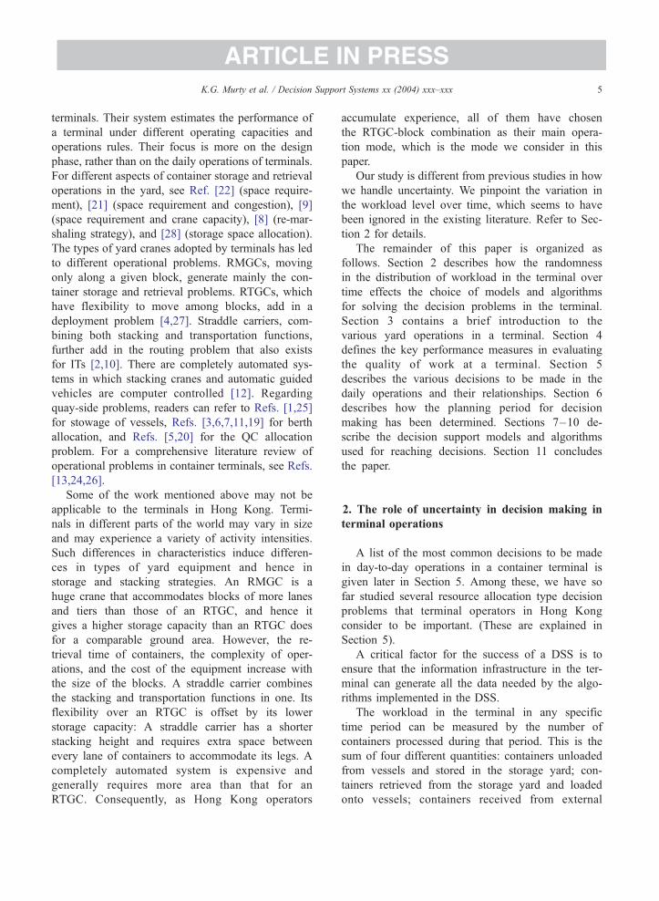
ARTICLE IN PRESSK.G. Murty et al. / Decision Support Systems xx (2004) xxx–xxx 5
terminals. Their system estimates the performance of
a terminal under different operating capacities and
operations rules. Their focus is more on the design
phase, rather than on the daily operations of terminals.
For different aspects of container storage and retrieval
operations in the yard, see Ref. [22] (space require-
ment), [21] (space requirement and congestion), [9]
(space requirement and crane capacity), [8] (re-mar-
shaling strategy), and [28] (storage space allocation).
The types of yard cranes adopted by terminals has led
to different operational problems. RMGCs, moving
only along a given block, generate mainly the con-
tainer storage and retrieval problems. RTGCs, which
have flexibility to move among blocks, add in a
deployment problem [4,27]. Straddle carriers, com-
bining both stacking and transportation functions,
further add in the routing problem that also exists
for ITs [2,10]. There are completely automated sys-
tems in which stacking cranes and automatic guided
vehicles are computer controlled [12]. Regarding
quay-side problems, readers can refer to Refs. [1,25]
for stowage of vessels, Refs. [3,6,7,11,19] for berth
allocation, and Refs. [5,20] for the QC allocation
problem. For a comprehensive literature review of
operational problems in container terminals, see Refs.
[13,24,26].
Some of the work mentioned above may not be
applicable to the terminals in Hong Kong. Termi-
nals in different parts of the world may vary in size
and may experience a variety of activity intensities.
Such differences in characteristics induce differen-
ces in types of yard equipment and hence in
storage and stacking strategies. An RMGC is a
huge crane that accommodates blocks of more lanes
and tiers than those of an RTGC, and hence it
gives a higher storage capacity than an RTGC does
for a comparable ground area. However, the re-
trieval time of containers, the complexity of oper-
ations, and the cost of the equipment increase with
the size of the blocks. A straddle carrier combines
the stacking and transportation functions in one. Its
flexibility over an RTGC is offset by its lower
storage capacity: A straddle carrier has a shorter
stacking height and requires extra space between
every lane of containers to accommodate its legs. A
completely automated system is expensive and
generally requires more area than that for an
RTGC. Consequently, as Hong Kong operators
accumulate experience, all of them have chosen
the RTGC-block combination as their main opera-
tion mode, which is the mode we consider in this
paper.
Our study is different from previous studies in how
we handle uncertainty. We pinpoint the variation in
the workload level over time, which seems to have
been ignored in the existing literature. Refer to Sec-
tion 2 for details.
The remainder of this paper is organized as
follows. Section 2 describes how the randomness
in the distribution of workload in the terminal over
time effects the choice of models and algorithms
for solving the decision problems in the terminal.
Section 3 contains a brief introduction to the
various yard operations in a terminal. Section 4
defines the key performance measures in evaluating
the quality of work at a terminal. Section 5
describes the various decisions to be made in the
daily operations and their relationships. Section 6
describes how the planning period for decision
making has been determined. Sections 7–10 de-
scribe the decision support models and algorithms
used for reaching decisions. Section 11 concludes
the paper.
2. The role of uncertainty in decision making in
terminal operations
A list of the most common decisions to be made
in day-to-day operations in a container terminal is
given later in Section 5. Among these, we have so
far studied several resource allocation type decision
problems that terminal operators in Hong Kong
consider to be important. (These are explained in
Section 5).
A critical factor for the success of a DSS is to
ensure that the information infrastructure in the ter-
minal can generate all the data needed by the algo-
rithms implemented in the DSS.
The workload in the terminal in any specific
time period can be measured by the number of
containers processed during that period. This is the
sum of four different quantities: containers unloaded
from vessels and stored in the storage yard; con-
tainers retrieved from the storage yard and loaded
onto vessels; containers received from external

ARTICLE IN PRESS
Fig. 4. The flow of outbound containers. SY= Storage Yard.
Underneath each location or operation, we list the equipment that
handles the containers there.
K.G. Murty et al. / Decision Support Systems xx (2004) xxx–xxx6
customer trucks and stored in the storage yard; and,
finally, containers picked up by external customers
from the storage yard. Each of these quantities for
any future time period is subject to many uncer-
tainties in terminal operations (arrival and departure
times of vessels depend on uncertainties posed by
weather; arrivals of customers’ trucks at the termi-
nal gates are subject to uncertain traffic conditions
on Hong Kong roads, which face congestion at
certain times).
Even after obtaining a reliable estimate of the total
workload for a time period, we have noticed that a
solution to a decision problem from a deterministic
optimization model based on the total workload esti-
mate performs well when implemented, only if this
workload is evenly distributed over the time period. In
reality, the workload in terminals quite often tends to
be unevenly distributed over time (when a vessel’s
processing is nearing completion and its departure
time is approaching, the workload undergoes a discrete
change in a very short time interval). For this reason,
we have found it necessary to develop approaches that
react well to momentary changes in the workload level
over time. Our choice of the model for a decision
problem and the algorithm for solving it has to
accommodate uncertainty in working conditions,
which is always there.
2.1. The special nature of terminal work
The workload in container terminals has the fol-
lowing special features:
(1) As described above, the distribution of the
workload over time tends to be uneven due to
many uncertainties in weather, traffic conditions
on roads, etc.
(2) It is not always possible to control the order in
which work comes, or the exact time of its arrival.
(3) Work has to be carried out when it arrives; its
processing cannot be delayed under ordinary
circumstances.
It is thus essential to choose models for problems
and algorithms that take all the above features into
account and that are practically intuitive and easy to
implement and maintain by the user’s operations and
information system teams.
3. The yard operations
3.1. The functions of a container terminal
A container terminal serves as an interface between
ocean and land transportation. Its main functions are:
� to receive outbound containers from shippers for
loading onto vessels and to unload inbound
containers from vessels for picking up by con-
signees; and� temporary storage of containers between ocean
passage and land transportation.
3.2. The flows of outbound and inbound containers
Outbound containers brought in by customer XTs
enter the terminal through the Terminal Gatehouse
(TG) where each container and its documentation are
checked. The TG then instructs the XT to proceed to
the storage block where the container will be stored
until the vessel into which it will be loaded arrives.
The RTGC working at that block removes the con-
tainer from the XT and puts it in its storage position.
When the time to load comes, the RTGC retrieves the
container from the stored position, puts it on an IT,
which takes it to a QC for loading onto the vessel. The
flow of outbound containers is represented in Fig. 4.
The flow of inbound containers has the reverse
features as indicated in Fig. 5.
3.3. How is a containerized vessel organized?
On a vessel, containers are stacked lengthwise along
the length of the vessel. Along its length, the vessel is

ARTICLE IN PRESS
Fig. 5. Flow of inbound containers.
K.G. Murty et al. / Decision Support Systems xx (2004) xxx–xxx 7
divided into segments, known as hatches or holds or
bays. Each of these can accommodate one 40-ft or two
20-ft containers along its length. In each hatch, up to 20
containers may be stacked in a row across the width of a
large vessel. The number of hatches in a vessel may be
over 20 depending on its total length. Some of the big
vessels may carry over 7000 TEUs. A vessel may call
on 5–10 ports in a voyage. For quick unloading and
loading, they usually assign containers to hatches
according to ports of call. When the vessel is docked
on the berth, several QCs work on it simultaneously,
with each QC working on a separate hatch. A QC itself
is wider than a hatch. Different QCs cannot work on
adjacent hatches at the same time.
A QC has four legs arranged in two rows of two
legs each. The space between the two rows is divided
into five truck lanes. While the QC is working on a
vessel, it has a set of ITs serving it (either taking away
the containers unloaded by the QC, or bringing
containers to be loaded into the vessel by the QC).
The ITs serving a QC always line up in one of the
lanes between the two rows of legs of the QC. Each of
these five lanes is assigned exclusively for the use of
the ITs serving one of the QCs working on the vessel
for the sake of safety and smooth operation. The
number of QCs that can work on a vessel is usually
limited by the number of these lanes. Normally, three
or four QCs work on a vessel simultaneously.
The unloading and loading sequence of containers
is usually determined by a special algorithm to make
sure that the docked vessel’s balance is not affected
while it is on the berth.
Fig. 6. Four containers stored in a stack.
3.4. RTGC operations
The RTGCs are expensive equipment (each costs
about US$850,000 at today’s prices) whose proper
utilization is very critical to the efficiency of container
handling operations in the storage yard.
The RTGCs move containers from ITs or XTs and
put them in their storage locations, and they retrieve
stored containers and put them on ITs or XTs. ITs and
XTs that arrive at a block to deliver or pick up a
container queue in the truck passing lane of the block
until the RTGC working in that block can serve them.
Thus, if RTGCs are not efficient in their work, there
may be truck congestion on the road near the block
and inside the block itself. Also, if the RTGC holds up
the ITs serving a QC working on a vessel, the QC may
have to wait, resulting in a delay in unloading or
loading the vessel.
There are two types of container retrieval opera-
tions of an RTGC:
� A productive move: When a container is moved
directly from its storage location to an IT or XT
waiting to pick it up, this is a productive move. For
example, retrieving the top container, A, from the
stack of four stored containers shown in Fig. 6 is a
productive move.� An unproductive or reshuffling move: When the
movement of a container, say A, becomes necessary
to retrieve another container stored underneath it in
the same stack, this is an unproductive move. In this
reshuffling move, container A is placed in another
stack in the same bay and may be put back in the
Fig. 7. Top view of a block B1 being served by an RTGC. Adjacent
block B2 shares a width line with B1; adjacent block B3 shares a
length line with B1.
ARTICLE IN PRESSK.G. Murty et al. / Decision Support Systems xx (2004) xxx–xxx8
original stack after the desired container is retrieved.
For example, to retrieve container C in Fig. 6,
containers A and B, stored above C, have to be
moved away first in reshuffling moves.
The number of reshuffling moves depends on the
strategy used for allocating storage spaces to arriving
containers.
Repositioning an RTGC from one block to another
is slow. If two blocks are adjacent by width (as B1 and
B2 in Fig. 7), the RTGC can move between them
without any turning motion. To move to an adjacent
block by length (as B1 and B3 in Fig. 7), the RTGC has
to come to the road on one end of the block, make a 90jturn of its wheels, then move on the road parallel to the
width line to the correct position for the adjacent block,
make another 90j turn, and enter that block. These 90jturns take extra time and also obstruct traffic on the
road for the time that the RTGC is on the road.
4. Key performance measures of a container
terminal
Container terminals work under multiple opera-
tional objectives. The most critical performance mea-
sure for rating the terminals is the ship turnaround
time (also called the port time of the ship), which is
the average time the terminal takes to unload and load
a docked vessel. This important objective function
must be minimized.
Closely related to the ship turnaround time, another
important measure is the average QC rate, which is
the quay cranes’ throughput measure during a period,
given by
QC rate
¼ no: of containers unloaded; loaded
total no: of QC hours of all QCs that worked:
In Hong Kong, as well as in some other places,
terminals charge shipping companies for every con-
tainer loaded into or unloaded from the vessel. Thus,
the QC rate must be maximized.
Note that these two measures are used internally by
a terminal to calibrate its own performance. In the
same terminal, with the same equipment, as the QC
rate goes up, the ship turnaround time goes down, and
vice versa. However, if the terminal acquires new QCs
and puts them in use, its ship turnaround time may go
down even without the QC rate changing.
The superior performance of Hong Kong’s termi-
nals can be seen from the following comparisons: In
2000, 6.6 million TEUs were handled by two Hong
Kong terminals, Hongkong International Terminals
(HIT) and COSCO-HIT, using 122 ha of land. Around
the same time (2001), Delta Terminal in the Nether-
lands, the busiest terminal in Europe, handled 2.5
million TEUs, using 280 ha of land, and the port of
Long Beach, one of the busiest container ports in the
United States, handled 4.6 million TEUs, using 295
ha of land.
On average, a QC in Hong Kong can handle over
30 containers per hour. Also, terminals in Hong Kong
seem to be always ready to invest in acquiring
adequate numbers of QCs to keep their ship turn-
around times short. This explains why terminals in
Hong Kong are considered among the most efficient
in the world.
As we will discuss in Section 5, the daily oper-
ations of terminals require a lot of inter-related deci-
sions. The very large number of decisions involved,
the multi-objective nature of the problem, the uncer-
tainty, and the complexity of the decisions, make it
impossible to derive answers to all the decisions by
solving a single mathematical model. The only prac-
tical way to obtain reasonable answers to these
decision problems is to study each of them separately
in a hierarchical fashion. We found the technique
called hierarchical decomposition with substitute ob-
jective functions for each stage developed in [16] very
useful in handling these decision making problems.
This is the basis for our DSS. Generally, the substitute
objective functions are consistent with the key per-
formance measure, i.e., they help reduce the ship
turnaround time and increase the QC rate.
4.1. A quantitative measure of congestion on the
roads inside the terminal
With so many trucks operating, the roads in the
terminal may get congested. Congestion slows the
trucks from carrying out their operation of transporting
containers from one location to another. This has an
undesirable effect on truck utilization and, more impor-
tantly, on the time taken to process the vessels. Hence,

ARTICLE IN PRESSK.G. Murty et al. / Decision Support Systems xx (2004) xxx–xxx 9
another important measure of performance is conges-
tion on the roads in the terminal, which must be
minimized.
Congestion is an easily recognized intuitive concept
in city traffic. Usually, in the street network of a city,
there may be arcs of different capacities. The average
speed and the standard deviations of speeds of vehicles
on different arcs may be very different; and there may
be different types of vehicles flowing on the arcs at the
same time. That is why developing a good measure of
congestion in city traffic is a difficult task.
4.1.1. The special nature of the road network inside a
terminal
Inside a terminal, however, both the road network
and the traffic on it have a special nature. All the roads
have the same traffic capacity and the traffic on them
consists of mostly trucks transporting containers. The
average speeds and the standard deviations or range
widths of speeds on all the roads are the same. It is thus
comparatively easier to develop a specialized quanti-
tative measure for congestion on the roads inside a
terminal in terms of the decision variables that can be
controlled in terminal operations.
We represent the gate, the berths, the blocks, and
all road intersections as nodes in a network. A road
segment is a portion of a road joining two such nodes.
If the road is two-way, each direction of it is consid-
ered to be a separate road segment. Thus, each road
segment can be traveled in only one direction and can
be represented by a directed arc joining the two nodes
on it. This leads to the representation of the road
system inside the terminal as a directed network,
which we denote by G.
We will measure flows on arcs in G in units of
trucks traveling through those arcs per unit time. Let s
denote the number of arcs in G, and for k = 1 to s, let
fk ¼ flow ðnumber of trucks traveling=unit timeÞ on the kth arc:
As the number of containers handled by the termi-
nal increases, flows on the arcs in G are expected to
increase. We are interested in a measure of congestion
in the whole road network, G, rather than on particular
arcs. Define
h ¼ Maxf fk : k ¼ 1; . . . ; sg;l ¼ Minf fk : k ¼ 1; . . . ; sg:
Since congestion is associated with high values
of flows on arcs, given the special nature of our
network G, h is a natural measure of congestion in
G. In reality, it is not only the value of h, but thenumber of arcs with such high flow values that
characterizes the quality of the traffic situation
inside the terminal. Minimizing h as the measure
of congestion does not provide any control on how
many arcs in G are subject to such high flow
values.
For a given volume of containers handled, we
can expect the best traffic situation to prevail if the
flows along the various road segments are as close
to each other as possible, because in this case, the
necessary traffic load is distributed among all the
road segments as much as possible instead of being
concentrated on just a few. Another measure of
congestion in the road system inside the terminal
is therefore h� l, and minimizing h� l may lead
to a better overall traffic situation than minimizing
only h.We will use h, h� l as the measures of congestion
to minimize. We will also consider the idea of adopt-
ing schemes that help distribute the traffic inside the
terminal equally along the various road segments in
order to alleviate the congestion.
4.2. Other important measures of performance to
optimize
Some of the other measures of performance to be
optimized are given below.
� The average waiting time of XTs that come to the
terminal to deliver outbound containers or pick up
inbound containers (to be minimized).� The average waiting time of the ITs in queues at
the QC and RTGC waiting to be serviced (to be
minimized).� The waiting time of the QC waiting for an IT (to be
minimized).� The volume of unproductive moves in the storage
yard (to be minimized).� The total number of ITs used in the various shifts
each day (to be minimized).
Optimizing all these performance measures re-
quires good resource allocation decisions, i.e., alloca-

ARTICLE IN PRESSK.G. Murty et al. / Decision Support Systems xx (2004) xxx–xxx10
tion and scheduling of berths and QCs to docked
vessels, allocation of storage spaces to containers,
deployment of RTGCs among blocks, allocation of
ITs to QCs and allocation of routes to traveling XTs
and ITs, in order to achieve a smooth and orderly flow
of containers between the gatehouse, the storage yard,
and the quayside.
5. Decisions to be made in daily operations
There are a variety of decisions to be made each
day. These are listed below.
D1. Allocation of berths to arriving vessels:
Allocate berths to arriving vessels to minimize
ship waiting time, port cost, and the dissatisfaction
felt by vessel’s captains about berthing order; and
to maximize utilization of berths and QCs.
D2. Allocation of QCs to docked vessels: Develop
a plan to allocate and schedule QCs to work on
docked vessels. This decision influences the turn-
around time of the vessels and the throughput rate
of the terminal.
D3. Appointment times to XTs: Ideally, all custom-
ers book the time to deliver outbound containers, or
to come to pick up their inbound containers, by
calling beforehand and making appointments.
Develop simple online decision rules to generate
these appointment times when they call, to help to
minimize XT waiting time and congestion in the
road network.
D4. Routing of trucks: Develop an algorithm to
route XTs and ITs inside the terminal to minimize
congestion on the roads.
D5. Dispatch policy at the TG and the dock:
Develop an online procedure for dispatching XTs
arriving at the TG with an outbound container and
ITs carrying an inbound container at the berth to
the blocks in the storage yard, to minimize
congestion at the blocks and congestion on the
roads.
D6. Storage space assignment: Assign storage
spaces to arriving containers to minimize reshuf-
fling volume and congestion on the roads.
D7. RTGC deployment: Determine how many
RTGCs should work in each block and when to
move an RTGC from one block to another. This
decision influences the port time of vessels and the
waiting times of QCs, XTs, and ITs.
D8. IT allocation to QC: Determine how many ITs
to allocate to each working QC to minimize the
vessel turnaround time and the waiting times of ITs
and the QC.
D9. Optimal IT hiring plans: Estimate IT require-
ments in each half-hour interval of the day and
develop a plan to hire ITs to meet these require-
ments, to minimize the total number of ITs hired
each day and to maximize IT utilization.
The decisions pertaining to containers have to be
made for each container as it goes through different
stages on its path through the terminal. The operations
of terminals are triggered by vessels. A terminal first
receives the information on a vessel a few weeks
before its actual arrival time. The terminal makes
temporary allocations of berth (D1) and of QCs
(D2) to the vessel based on its projected workload.
XTs with appointment times (D3) start to bring in
export containers for the vessel a few days before the
actual vessel arrival. These containers are dispatched
for storage in blocks (D5), depending on the situation
in the yard at the time of their arrivals. A container
allotted to a block is then assigned to a storage stack
(D6) where it requires the minimum number of
reshuffles.
The actual workload and the likely vessel arrival
time are known about a day or so before the actual
vessel arrival. The actual berth allocation (D1) and
QC allocation (D2) are determined based on this
information. With more updated total workload
requirements, the terminal determines the total
number of ITs (D9) to be hired on the following
day and formulates the preliminary plan of assign-
ing ITs to QC (D8). D5 also has an influence on
D8 and D9.
During the actual operations, the terminal makes
real-time decisions on the allocation of ITs to QC
(D8), the movement of yard cranes among blocks
(D7), and the routing of ITs between QC and blocks
(D4). All the other planned decisions as described
above are also subject to changes according to real-
time activities at the terminal.
The development of a DSS to make all these
decisions optimally is an ongoing effort. So far, we
have investigated strategies for making decisions D4

ARTICLE IN PRESSK.G. Murty et al. / Decision Support Systems xx (2004) xxx–xxx 11
to D9 because these decisions involve resource plan-
ning issues in the storage yard, which are issues of
primary interest to the terminals in Hong Kong.
6. The planning period and input data for decision
making
Container terminals work three 8-h shifts around
the clock, every day. It is convenient to make the
planning period for decision making equal to the time
interval of a shift, or less.
There are two important considerations for
selecting the appropriate length of the planning
period. One is that it should be possible to estimate
the total workload in the period with reasonable
accuracy. Another is that this total workload should
be distributed as uniformly as possible over time
during this period. Operators have found that a 4-
h period (i.e., half of a shift) comes closest to
meeting both these considerations adequately. With
shorter time periods, the accuracy of the estimate of
total workloads is poor. With longer time periods,
the distribution of the workload over time tends to
be uneven. Hence, terminals have found it conve-
nient to organize their work with a 4-h period as
the planning period for decision making. A day is
divided into six planning periods: 00:00–4:00,
4:00–8:00, 8:00–12:00, 12:00–16:00, 16:00–
20:00, and 20:00–24:00. Activities spanning across
more than one time period have their associated
quantities, such as workload and equipment de-
mand, shared across the time periods according to
the amount of time that the activity requires.
Towards the end of each period, the terminals use
the latest information available for the following
period to formulate a plan for operations in that
period.
The terminals in Hong Kong have advanced infor-
mation systems that keep real-time information on
container flows and the status of various resources in
them. This information is not only essential for
tracking the containers for security and customs
reasons, it also provides reliable input data for deci-
sion making. While the data needed for each decision
problem will be mentioned in the section for that
decision, here, we give a brief overview of the types
of data and their sources.
There are two types of input data for the
decisions: static and dynamic. Static data are the
system parameters that (generally) hold constant
throughout any planning horizon, e.g., the road
network in the yard, the number and capacities of
the blocks, the numbers of quay cranes and yard
cranes, etc. They are readily accessible from data-
base records whenever needed. Dynamic data re-
flect the status (values) of variables that change
with operations, e.g., the current positions of equip-
ment, the number of containers stored in each
block, and the storage position of each container,
etc. These are all updated in real time and their
current values are available from the information
system.
Changes to the dynamic data are triggered by
the arrivals and departures of containers into/from
the terminal. On the gate side, the times of con-
tainer arrivals and departures are determined when
the customers make appointments for dropping off
or picking up the containers. On the quayside, long
before a vessel arrives, information on the estimat-
ed arrival time, the number of containers to be
unloaded at a Hong Kong terminal and their exact
positions on the vessel is sent electronically to the
terminal by the carrier. The carrier also gives the
terminal details on the containers to be loaded into
the vessel and the hatch into which each of them
should go, based on its destination port, without
restricting the specific position in the hatch for
every individual container. Based on all the car-
riers’ information, the terminals operations planner
makes an unloading/loading work plan (the sequen-
ces of unloading and loading containers), using a
special-purpose software. The vessel’s arrival time
and this unloading/loading plan determine the ar-
rival times of inbound containers from the vessel
and the departure times of the outbound containers
to the vessel. With modern communication tools,
fairly accurate vessel-related data are available in
advance for planning decisions. The data on the
gate side are not always known in advance pre-
cisely because some customers do not make ap-
pointments before dropping off or picking up
containers. For planning purposes, we estimate the
number of such container arrivals and departures in
future periods based on the distributions of past
data.

ARTICLE IN PRESSK.G. Murty et al. / Decision Support Systems xx (2004) xxx–xxx12
7. Storage space assignment, dispatching policy at
the TG and the berth, and the routing of trucks in
the storage yard
Since storage spaces are sources and destinations
for truck travel within the terminal, the three deci-
sions on storage space assignment, the policy to be
followed at the TG and the berth for dispatching
XTs and ITs, and the routing of trucks are highly
inter-related, and we study them together.
The planning period for these decisions is a 4-
h period (the beginning or the ending half of a
shift) as discussed in Section 6. The input data
needed for the models consists of: the road network,
G (discussed in Section 4), the appointment time
database (a list of customers who have been given
appointments during the planning horizon, a list of
the outbound containers they are expected to drop
off, and a list of the inbound containers in storage
they are expected to pick up), the vessel schedule
data (the arrival time, workload), the vessel unload-
ing and loading plans, and other data as listed
below.
b=Number of berths in the terminal.
m =Number of blocks in the yard.
ki= Storage capacity of block i (in number of
containers), i = 1 to m.
ESi( p) =Number of outbound containers stored in
block i to be retrieved during period p for loading
onto vessels, i= 1 to m.
ESid( p) =Number of containers among ESi( p) that
have to go to berth d, d = 1 to b.
ESðpÞ ¼Pm
i¼1 ESiðpÞ, total number of stored
outbound containers to be retrieved during period
p for loading onto vessels.
ISi( p) =Number of inbound containers in storage
in block i expected to be retrieved during period p
for pickup by customers, i= 1 to m.
ISðpÞ ¼Pm
i¼1 ISiðpÞ = total number of inbound
containers to be picked up by customers during
period p.
IM( p) = Total number of inbound containers
expected to be unloaded from vessels during
period p.
IMd( p) =Number of inbound containers to be
unloaded from vessels docked at berth d, d = 1 to
b. We havePb
IMdðpÞ ¼ IMðpÞ.
d¼1EX( p) = Number of outbound containers ex-
pected to be brought in for storage during
period p.
XITi(t) =Number of XTs and ITs waiting in block i
for receiving service from the RTGC of block i, at
the time of observation t.
7.1. Storage space allocation decisions for the next
period, p+1
Let p be the current period. We discuss procedures
for making storage allocation decisions for containers
arriving in the next period, p + 1.
Each of the IM( p + 1) + EX( p + 1) new containers
arriving at the terminal during period p + 1 has to be
assigned a specific storage space in the yard for
storage. Ideally, the assignment policy could have an
impact on the congestion in the road network, at the
blocks, and on the total volume of reshuffling, all of
which must be minimized.
There are a large number of container storage
positions in the yard, some of which are already
occupied by containers in storage at the beginning
of this period. Determining a specific open storage
position for each of the newly arriving IM( p + 1) +
EX( p + 1) containers leads to a huge mathematical
model that will be impractical to solve. In Ref.
[15,18], this storage space assignment decision has
been divided into three stages.
7.1.1. Stage 1: block assignment
Determine the container quota for block i, which is
the number of containers among the arriving EX
( p + 1) + IM( p + 1) that will be stored in block i. This
determination leads to the following decision varia-
bles for this stage:
xi( p + 1) =Container quota number for block i
during period ( p + 1) = the total number of out-
bound and inbound containers arriving at the
terminal in this period to be stored in block i,
i = 1 to m.
Stage 1 determines only the container quota
numbers for the blocks, not the identities of contain-
ers which will be stored in each block. The identities
will be determined by the dispatching policy dis-
cussed in Stage 2.
ARTICLE IN PRESSupport Systems xx (2004) xxx–xxx 13
7.1.2. Stage 2: dispatching policy at the TG and the
docks
Determine a policy that TG and dock supervisors
will follow to dispatch XTs and ITs to the blocks in
the storage yard, so that by the end of the period, the
number of new containers that each block gets for
storage is equal to its quota number determined in
Stage 1, while minimizing congestion at the blocks
and on the roads.
The reason for a good dispatching policy can be
explained this way. Suppose the container quota for
block 1 is 13. If the TG sends 13 of the arriving XTs
consecutively one after the other to block 1, then
serious congestion will take place at block 1 right
away. The dispatching policy should ensure that
consecutive trucks in the arriving stream are dis-
patched to different blocks that are widely dispersed
in the storage yard, so that each block has adequate
time to process the truck reaching it before the next
truck sent to this block arrives there. Also, the
dispatching policy should distribute these trucks in
all directions to ensure that the truck traffic on the
roads is evenly distributed in all directions.
7.1.3. Stage 3: storage position assignment
For each container arriving at block i for storage,
determine the optimal available position in the block
for storing it to minimize the incidence of reshuffling
it when retrieving the containers underneath it.
7.2. A multicommodity network flow approach to the
Stage 1 storage problem (block assignment)
Given EX( p + 1), IMd( p + 1), ESid( p + 1), ISi
( p + 1), the problem of determining the values of the
decision variables, xi( p + 1) for i = 1 to m, to minimize
congestion on the road network (measured either by h,or h� l) has been formulated in Ref. [15] as a
multicommodity network flow problem on the net-
work G. This problem can easily be solved, since it is
a linear program, by using a commercial software
package like CPLEX. This problem is solely based on
the estimated total workload during period ( p + 1). We
found that the solution to this problem works well in
practice as long as the workload is distributed more or
less uniformly over time. The solution is poor during
periods in which the workload distribution over time
is uneven.
K.G. Murty et al. / Decision S
In Ref. [15], an alternative approach to this prob-
lem that adapts quite well to momentary changes in
the workload level is developed. We discuss that
approach next.
7.3. A fill ratio equalization approach to the Stage 1
storage problem (block assignment)
The alternative approach developed in Ref. [15]
for block assignment is based on the following
hypothesis.
Hypothesis : Assuming that the dispatching policy
developed in Stage 2 disperses consecutive trucks in
the arriving stream all around the storage yard, traffic
congestion in the terminal will be at its minimum (i.e.,
the traffic volume will tend to be equally distributed
on all the road segments and the blocks in the
terminal) if the fill ratios of all the blocks are
maintained to be nearly equal.
Applying this hypothesis leads to the following
very simple procedure for determining the Stage 1
decision variables, xi( p + 1) for i= 1 to m for next
period p + 1. Here,
xi( p) is the container quota number for block i in
period p,
Fi( p) is the fill ratio of block i at the beginning of
period p,
q( p) is the fill ratio for the whole storage yard
(including all the blocks) at the beginning of period
p,
Gi( p) is the number of containers stored in block i
at the beginning of period p; for i = 1 to m.
7.3.1. Procedure for Stage 1 (container quota number
determination) for period p+1
Here is a summary to help us understand the
calculations in the procedure. Step 1 uses the data
from the current period, p, to compute the fill ratios of
various blocks at the beginning of the next period
p+ 1. Step 2 uses these, the number of new containers
arriving, and the number of stored containers expected
to be retrieved during period p + 1 to compute the
container quota numbers for the various blocks in this
period to equalize the fill ratios in the various blocks
as much as possible by the end of the period (i.e., by
the beginning of period p + 2).

ARTICLE IN PRESS
Table 1
Illustration of Step 2
Data Computed results
i ki Ai qkiq( p+ 2)a xi( p+ 1)
1 600 100 452 352
2 600 120 452 332
3 550 150 414 264
4 550 300 414 92
5 500 325 376 0
6 500 350 376 0
7 500 375 376 0
8 500 400 376 0
9 500 450 376 0
EX( p+ 1) + IM( p+ 1) = 1040
Ai=Gi( p+ 1)� (ESi( p+ 1) + ISi( p+ 1))
K.G. Murty et al. / Decision Support Systems xx (2004) xxx–xxx14
Step 1. Compute the fill ratios of the blocks at the
beginning of period p+1.
Fiðpþ 1Þ ¼ ðGiðpþ 1Þ=kiÞ
¼ ðFiðpÞki � ESiðpÞ � ISiðpÞ þ xiðpÞÞ=ki:
Step 2. Computing the container quota numbers
xi( p+1) for blocks in period p+1. The fill ratio in
the whole storage yard at beginning of period p + 2
(i.e., the end of period p + 1) will be
qðpþ 2Þ
¼
Xmi¼1
Giðpþ 1Þ � ðESðpþ 1Þ þ ISðpþ 1ÞÞ þ EXðpþ 1Þ þ IMðpþ 1Þ
Xmi¼1
ki
:
Therefore, q( p + 2) can be computed from the
available data at the beginning of period p + 1. The
fill ratio equalization approach determines the con-
tainer quota numbers for blocks xi( p + 1) so that the
fill ratios for all the blocks come as close to q( p + 2)as possible by the end of period p + 1. This leads to the
following linear programming (LP) model (the varia-
bles in this LP are xi( p + 1), ui+, ui
�; all other symbols
denote known data elements):
MinimizeXmi¼1
ðuþi þ u�i Þ
subject to
½Giðpþ1Þ�ðESiðpþ1ÞþISiðpþ1ÞÞ� þ xiðpþ1Þþuþi � u�i¼kiqðpþ 2Þ; all i
Xmi¼1
xiðpþ 1Þ ¼ EXðpþ 1Þ þ IMðpþ 1Þ
all xiðpþ 1Þ; uþi ; u�i z0:
The optimal solution of this LP model leads to the
following scheme.
Let c( p + 1) = EX( p + 1) + IM( p + 1) initially. This
is the number of new containers arriving in period
p + 1 to be allotted to the blocks for storage.
Rearrange the blocks in increasing order of Gi
( p + 1)� (ESi( p + 1) + ISi( p + 1)), i.e., after rearrange-
ment, this quantity will be increasing in the order i= 1
to m. In this order i = 1 to m, carry out
1 . x i ( p + 1 ) = m in{max{0 , qk iq( p + 2 ) a� [ G i
( p + 1)� (ESi( p + 1) + ISi( p + 1))]}, current value
of c( p + 1)}.
2. New value of c( p + 1) = current value of c( p + 1)
� xi( p + 1).
3. If i <m, increment i by 1 and go back to Step 1.
This provides the broad outline of the procedure
for determining xi( p + 1). Container terminals do
make heuristic modifications to this general proce-
dure according to their preferences and any special
circumstances.
We provide a numerical example to illustrate Step
2. In this example, we consider a storage yard con-
sisting of only nine blocks. For blocks i = 1 to 9, data
on ki, Ai=Gi( p + 1)� (ESi( p + 1) + ISi( p + 1)) are giv-
en in Table 1.
In this numerical example, EX( p + 1) + IM( p + 1) =
1040. The fill ratio in the whole storage yard at the
end of period p + 1 will be
qðpþ 2Þ ¼ ð2570þ 1040Þ=4800 ¼ 0:752:
The blocks are already in increasing order of Ai,
i = 1 to 9. The computed values of the quota numbers,
xi( p + 1), are given in Table 1.
This algorithm assigns 1040 containers arriving for
storage in period p + 1 to blocks i = 1 to 9 in that order,
bringing the expected number of stored containers in
this block at the end of period p + 1 to kiq( p+ 2), until

ARTICLE IN PRESSK.G. Murty et al. / Decision Support Systems xx (2004) xxx–xxx 15
all these containers are assigned. Notice that the above
procedure only determines the values of the decision
variables xi( p + 1), i = 1 to m; it does not assign each
specific arriving container to a storage block. Once the
period begins, arriving containers are assigned to
blocks by the following online procedure that helps
to even out the traffic to the blocks and along the roads.
7.4. Online dispatching procedure for assigning
containers to storage blocks during a period (Stage 2)
Sending too many XTs or ITs to a block in a short
period of time creates congestion at that block. To
avoid this, the following truck dispatching policy is
used at the TG and the berths.
7.4.1. For outbound and inbound containers
When a new container arrives at time point t during
the period, either at the TG or from a QC at a berth,
the values of XITi(t) for those blocks with the current
value of xi( p + 1)>0 at that moment are examined, and
the container is assigned to the block with minimum
XITi(t). If there is a tie, the container is assigned to the
block with a higher xi( p + 1). Any further tie is broken
arbitrarily. After the container is assigned, the value of
xi( p + 1) is updated for that i, i.e., the new value of
that xi( p + 1) = the current value of that xi ( p+ 1)� 1
for the assigned block i. The values of XITi(t) are
updated in real time.
The terminals also make other heuristic modifica-
tions to this online block assignment procedure for
storage of arriving containers according to their
preferences.
To implement this dispatching policy, it is necessary
to set up a system that monitors how many trucks are
waiting in each block and to convey this information to
the TG and to the berth. In fact, each terminal operator
in Hong Kong has a centralized information system
with user terminals at the TG and inside the operator
cabinet on each YC and QC. Every container moving
between a truck and a QC and between a truck and a
block is monitored and its location is fed back to the
system. Hence, the real-time number of trucks waiting
in andmoving towards a block is readily available from
the system. The values of xi( p + 1) in the system are
also updated in real time. Therefore, it is convenient to
implement and embed the truck dispatching policy in
the information system. When a container arrives, the
operator at the TG or QC simply needs to inform the
system about its arrival; the system will use the dis-
patching policy to decide to which storage block the
container should go based on the real-time information
and convey the decision to the operator who then
directs the XT or IT driver accordingly.
7.5. Allocating storage spaces to containers within
blocks, the Stage 3 problem
Since we cannot control the order in which con-
tainers arrive for storage in a block and cannot hold
arrived containers before storage, only online algo-
rithms assigning positions to containers as they arrive
in the block are suitable for implementation.
The assignment of a storage position to a container
arriving in this block mainly impacts the total amount
of reshuffling in this block. These assignments have to
be made with the objective of minimizing the total
amount of reshuffling in this block.
A block consists of a number of stacks for storing
containers. Some of these stacks may already have
some containers stored in them. Others may be empty.
For each arriving container, we can make an esti-
mate of the time when it will be retrieved from storage.
7.5.1. For inbound containers in storage
Using the data on appointment times given to
customers, an estimate of the retrieval time of inbound
containers in storage can be obtained.
7.5.2. For outbound containers in storage
The expected time to retrieve an outbound con-
tainer in storage to load it into its vessel is obtained
using the data on vessel arrival times and the unload-
ing and loading sequences for them.
The storage position for an arriving container is
determined to minimize the number of reshuffling
moves that it may create. With tens of thousands of
storage location decisions to make in a day, the DSS
uses a simple decision tool, the reshuffle index. Define
the reshuffle index of an arriving container, A, for a
stack in the block that has space for storing it to be
0, if the stack is empty when A arrives for storage,
c = the number of stored containers in the stack
with estimated retrieval times before that of A,
otherwise.

ARTICLE IN PRESSK.G. Murty et al. / Decision Support Systems xx (2004) xxx–xxx16
The reshuffle index measures the number of times
that container A may have to be reshuffled if it is put
in storage in this stack at this time. It does not
consider the possible effect on reshuffling of contain-
ers coming at later times.
The problem of storing the containers assigned to
this block with the objective function of minimizing the
reshuffle indices of all the containers in their storage
positions is analogous to a bin packing problem with
the stacks playing the role of bins that can hold five (or
four, depending on the height of the RTGC serving this
block) containers. The main difference between this
problem and a traditional bin packing problem is that
the order of arrivals of containers is dynamic and
uncontrollable, and that the contribution of a container
to the objective function varies with the stack in which
it is stored. Under this analogy, we implement the
solution to this problem corresponding to the best fit
solution in bin packing. This leads to the online
procedure discussed below.
7.6. Online procedure for assigning storage positions
to containers arriving for storage in a block
When the container arrives, find the stack in the
block with an empty space that has the smallest
reshuffle index for it among all such stacks, breaking
ties in favor of the stack with the maximum number of
containers stored already. Store the container in the
top position of that stack.
This procedure has found acceptance from the
terminals as it is easy to implement with their infor-
mation infrastructures.
Several other strategies for this decision have been
proposed and analyzed in Ref. [26].
8. Optimal deployment of RTGCs among the
blocks
The RTGCs are a critical resource whose perfor-
mance in the storage yard influences the waiting times
of the XTs, ITs, and QCs, and, in turn, the port time of
vessels. As the workload in the various storage blocks
changes over time, deployment of RTGCs among
storage blocks in order to provide more RTGCs to
blocks with heavier workloads is an extremely impor-
tant issue in terminal operations management.
The planning horizon for the RTGC deployment
problem is also a 4-h period (the beginning or ending
half of a shift) as discussed in Section 6.
Because of the limited size of a block, there can be
at most two RTGCs working in a block at any time.
One of the big terminals in Hong Kong has 70 storage
blocks that need RTGCs and, on a typical day, has
around 95 RTGCs in working order to serve these
blocks. In a typical planning period, all the 70 blocks
will have some activity that requires an RTGC. It is
thus reasonable to assume that every block needs at
least one RTGC in every planning period for at least
part of the period. Some blocks with a lot of activities
may actually need two RTGCs to support the work in
them. Since there are not enough RTGCs to station
two in every block that needs them, it is necessary to
move them from blocks in which the workload is low
to those where it is high.
Since RTGC movement from one block to another
is slow and since this movement results in not only the
loss of productive time of the moving RTGC, but also
obstructs traffic on the roads between the blocks, the
terminals have adopted the policy that an RTGC can
move from one block to another at most once in each
period. Such a move can occur at any time within the
period.
As a period is 4 h long, the capacity of an RTGC in
a period can be stated as 240 RTGC minutes. From
observations in the storage yard, we determine
s = the average time in minutes that it takes an
RTGC to either stack a container in a column, or to
retrieve the stored top container from a column.
g = reshuffling frequency per productive move.
This is the average number of containers reshuffled
per container retrieved from storage, or the average
number of unproductive reshuffling moves per
productive move.
In terminals in Hong Kong, g has been observed to
be 1.17 reshuffling moves for each container
retrieved.
Given these observations, and the expected number
of containers to be stacked in and retrieved from a
block during a period, it is possible to measure the
RTGC workload in that block in that period in terms of
RTGC minutes. The RTGC deployment models use
this workload data for deployment decisions.

ARTICLE IN PRESSK.G. Murty et al. / Decision Support Systems xx (2004) xxx–xxx 17
It is very important that the RTGC workload in each
block in a period be finished in that period itself,
otherwise, this may result in excessive XT waiting
time or delay vessel departure times. An unfinished
RTGC workload will be carried over to the next
period. This will have to be finished during the first
part of the next period. We call the unfinished RTGC
workload in a block in a period the delayed RTGC
workload. The aim of RTGC deployment is to mini-
mize the total delayed RTGC workload in each period.
Besides the data elements s and g mentioned
above, RTGC deployment models for a period, p,
need ESi( p), ISi( p) defined in Section 7, xi( p) defined
and computed in Sections 7.1 and 7.3, and the
following data:
m =Number of blocks in the yard.
n =Total number of working RTGCs in the yard.
ri( p) =Number of RTGCs stationed in block i at
the beginning of period p, i= 1 to m.
cij =Time in minutes that it takes an RTGC to
move from block i to block j; for i, j= 1,. . .,m, andi p j. cij is set tol or a large positive number if the
terminal wants to forbid the movement of an
RTGC from block i to block j for any reason.
From this data, we can compute the expected
RTGC workload in block i in period p, measured in
RTGC minutes, to be
wiðpÞ ¼ ðESiðpÞ þ ISiðpÞÞð1þ gÞs þ xiðpÞs:
However, what makes the RTGC deployment
problem difficult is the following important fact.
Fact 1 (about RTGC workloads): If all the work of an
RTGC in a period is available to be carried out at the
beginning of the period, then the RTGC can quickly
finish it and move. Unfortunately, the RTGC work-
load in a period is usually not all available at the
beginning of the period. The need for an RTGC
occurs only when the trucks arrive in its block for its
service. Thus, the work to be carried out by an RTGC
is spread over the period as trucks arrive.
In Ref. [15], the RTGC deployment problem for a
single period and for minimizing the total delayed
workload has been modeled as an MIP (Mixed Integer
Programming) problem that can be solved quite
efficiently by commercial software packages like
CPLEX. Refs. [26,27] modeled the same problem
for six periods (a whole day) as a much larger MIP
and developed a special approach for solving the
problem efficiently based on Lagrangian relaxation.
One shortcoming of all these models is that they
ignore Fact 1 mentioned above.
If there is full-time work for an RTGC in the block
in which it is stationed at the beginning of period p,
that RTGC should continue to stay in the same block
during the entire period. We therefore first classify all
RTGCs in their current positions at the beginning of
period p into:
eligible RTGCs: those that can be moved from their
current blocks in period p;
ineligible RTGCs: those that will be kept in their
current blocks in period p.
Unfortunately, it is not a simple matter of com-
paring the workload, wi( p), in block i with the
available 240ri( p) RTGC minutes from the ri( p)
RTGCs stationed in this block at the beginning of
period p to determine whether some of these RTGCs
can be considered eligible, because of Fact 1. For this
reason, crane supervisors make decisions on which
RTGCs are eligible to move, based on the following
considerations.
(a) If a block has two RTGCs stationed in it at the
beginning of the period and after some time in the
period if the remaining workload in the block is
low enough that only one RTGC can handle it,
then one of these RTGCs is eligible to move from
this block at that time.
(b) If there is no remaining workload in a block after
some time in this period, then all the RTGCs in
this block are eligible to move from this block at
that time.
(c) An RTGC can move easily between a pair of
adjacent blocks that share a common width line. If
(B1,B2) is such a pair, and if the expected arrival
pattern of trucks in these two blocks during a
period is such that k ( = 1, 2, or 3) RTGCs in these
two blocks together can handle this workload by
moving between these two blocks freely, then any
RTGC in these two blocks put together beyond k
is eligible to move at the beginning of this period.

ARTICLE IN PRESS
Table 2
Travel time of eligible RTGCs to sink blocks (in minutes)
Eligible RTG Sink block
B1 B2 B3 B4 B5 B6 B7
RTGC 1 20 20 25 35 40 50 55
RTGC 2 25 10 20 30 35 45 50
RTGC 3 30 20 10 25 30 40 45
RTGC 4 35 25 20 20 25 35 40
RTGC 5 40 30 25 10 20 30 35
RTGC 6 45 35 30 20 10 25 30
RTGC 7 50 40 35 25 20 20 35
RTGC 8 50 40 35 25 20 20 35
RTGC 9 60 50 45 35 30 20 10
No. of eligible
RTGC needed
1 2 1 1 1 1 1
K.G. Murty et al. / Decision Support Systems xx (2004) xxx–xxx18
Crane supervisors use many such considerations to
determine which RTGC is eligible to move from its
initial block in this period and the time at which it can
move.
Also, block j in period p is classified as a sink block
if rj( p) = 1 or 0 and the expected workload in it exceeds
the capacities of these RTGCs. The expected number of
additional RTGCs it needs in this period, dj, is
dj= 1, if rj( p) = 1, because there can be at most two
RTGCs in a block at any time,
dj= 1 or 2, if rj( p) = 0, determined based on the
estimated workload in that block.
Let ne be the total number of eligible RTGCs in
period p; number them as RTGC 1 to RTGC ne.
Let ms be the number of sink blocks in period p;
number them as blocks 1 to ms. Define the decision
variable, xij, for i = 1 to ne, j= 1 to ms by
xij ¼1; if RTGC i moves to block j in period p;
0; otherwise:
8<:
Denote b(i) as the block in which eligible RTGC i
stays at the beginning of period p, thenPne
i¼1
Pms
j¼1
cbðiÞjxij measures the RTGC productive time lost in the
moves. This is like a substitute objective function for
the total delayed RTGC workload. Thus, the follow-
ing transportation problem is a suitable single period
model for RTGC deployment in that period when
nezSjdj.
MinimizeXnei¼1
Xms
j¼1
cbðiÞjxij
subject toXms
j¼1
xijV1; i ¼ 1; . . . ; ne
Xnei¼1
xij ¼ dj; j ¼ 1; . . . ;ms
xij ¼ 0 or 1; i ¼ 1; . . . ; ne; j¼1; . . . ;ms:
When ne <Sjdj, a similar transportation problem
can be formulated in which the RTGC constraints
hold as equality and the sink block constraints hold as
less than or equal to. Any of these transportation
problems can be easily solved to optimality. But the
strategy of using the more easily computed Vogel
solution [14] for it as a near optimum is simpler to
implement by the terminals.
For a numerical example, suppose that, in a certain
period, there are nine eligible RTGCs (RTGC1 to
RTGC9) and seven sink blocks (B1 to B7), where
sink block 2 needs two RTGCs in this period, and
each of the rest need one RTGC. Data on the travel
time in minutes of the eligible RTGCs to the sink
blocks is given in Table 2. In this numerical example,
the Vogel solution with a total cost of 115 min is in
fact an optimum solution of the transportation model.
The model has several alternative integer optimal
solutions. One of them is given by: x1,1 = x2,2 = x3,3 =
x4,2 = x5,4 = x6,5 = x7,6 = x9,7 = 1, and all other xij = 0.
9. Optimal allocation of ITs to QC
The workload of a QC working on a hatch of a
vessel can be estimated fairly accurately based on the
stowage situation of the inbound containers in the
hatch and by the stowage plan of the outbound
containers that go into that hatch. When a QC is
unloading containers from a docked vessel, a certain
number of ITs are allotted to it. These ITs queue up
under the QC. The QC unloads a container from the
vessel and puts it on the IT at the head of the queue.
That IT then takes the container to the storage block
where it is to be stored and queues up in the truck
ARTICLE IN PRESS
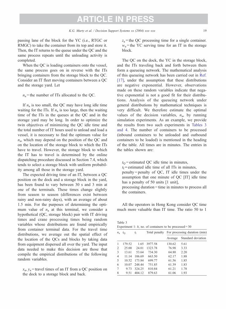
Table 3
Experiment 1: h, no. of containers to be processed = 30
na tQ tI Total penalty For processing duration (min)
Average Standard deviation
1 179.52 1.65 3977.58 130.62 5.61
2 25.00 24.01 1323.78 76.98 3.33
3 13.61 53.64 734.30 64.80 2.20
4 11.14 106.69 663.50 62.17 1.88
5 10.52 173.84 699.77 61.56 1.85
6 10.07 248.44 751.85 61.39 1.83
7 9.73 324.25 810.84 61.21 1.78
8 9.51 404.12 879.63 61.06 1.93
K.G. Murty et al. / Decision Support Systems xx (2004) xxx–xxx 19
passing lane of the block for the YC (i.e., RTGC or
RMGC) to take the container from its top and store it.
Then, the IT returns to the queue under the QC and the
same process repeats until the unloading activity is
completed.
When the QC is loading containers onto the vessel,
the same process goes on in reverse with the ITs
bringing containers from the storage block to the QC.
Consider an IT fleet moving containers between a QC
and the storage yard. Let
na = the number of ITs allocated to the QC.
If na is too small, the QC may have long idle time
waiting for the ITs. If na is too large, then the waiting
time of the ITs in the queues at the QC and in the
storage yard may be long. In order to optimize the
twin objectives of minimizing the QC idle time and
the total number of IT hours used to unload and load a
vessel, it is necessary to find the optimum value for
na, which may depend on the position of the QC and
on the location of the storage block to which the ITs
have to travel. However, the storage block to which
the IT has to travel is determined by the online
dispatching procedure discussed in Section 7.4, which
tends to select a storage block with uniform probabil-
ity among all those in the storage yard.
The expected driving time of an IT, between a QC
position on the dock and a storage block in the yard,
has been found to vary between 30 s and 3 min at
one of the terminals. These times change slightly
from season to season (differences exist between
rainy and non-rainy days), with an average of about
1.5 min. For the purposes of determining the opti-
mum value of na at this terminal, we consider a
hypothetical (QC, storage block) pair with IT driving
times and crane processing times being random
variables whose distributions are found empirically
from container terminal data. For the travel time
distributions, we average out the spatial effect of
the location of the QCs and blocks by taking data
from equipment dispersed all over the yard. The input
data needed to make this decision are those that
compile the empirical distributions of the following
random variables.
xa, ya = travel times of an IT from a QC position on
the dock to a storage block and back.
za = the QC processing time for a single container.
wa = the YC serving time for an IT in the storage
block.
The QC on the dock, the YC in the storage block,
and the ITs traveling back and forth between them
form a queueing network. The mathematical analysis
of this queueing network has been carried out in Ref.
[17], under the assumption that these distributions
are negative exponential. However, observations
made on these random variables indicate that nega-
tive exponential is not a good fit for their distribu-
tions. Analysis of the queueing network under
general distributions by mathematical techniques is
very difficult. We therefore estimate the optimal
values of the decision variables, na, by running
simulation experiments. As an example, we provide
the results from two such experiments in Tables 3
and 4. The number of containers to be processed
(inbound containers to be unloaded and outbound
containers to be loaded) is mentioned in the heading
of the table. All times are in minutes. The entries in
the tables shown are:
tQ = estimated QC idle time in minutes,
tI = estimated idle time of all ITs in minutes,
penalty = penalty of QC, IT idle times under the
assumption that one minute of QC [IT] idle time
has a penalty of 50 units [1 unit],
processing duration = time in minutes to process all
the containers.
All the operators in Hong Kong consider QC time
much more valuable than IT time. The ratio 50 to 1

ARTICLE IN PRESS
Table 4
Experiment 2: h, no. of containers to be processed = 60
na tQ tI Total penalty For processing duration (min)
Average Standard deviation
1 156.73 2.32 7838.68 258.79 8.18
2 47.87 29.14 2422.69 149.94 4.73
3 20.92 67.72 1113.75 122.95 3.16
4 13.90 147.70 842.52 115.80 2.47
5 12.30 261.25 876.30 114.34 2.20
6 11.91 386.90 982.58 114.23 2.33
7 11.49 516.07 1090.81 114.04 2.24
8 11.57 648.00 1226.62 114.12 2.38
K.G. Murty et al. / Decision Support Systems xx (2004) xxx–xxx20
has frequently been considered as the penalty for
idleness of these resources.
In both experiments, it can be seen that na = 4 ITs
allocated to the QC yielded the lowest penalty esti-
mate and very nearly the shortest processing duration
for all the containers.
The simulation experiments also give the estimated
expected time in minutes to process a hatch, and the
standard deviation of this time as functions of h,
where h is the number of containers to be processed
in this hatch. These quantities corresponding to the
optimum value of na are used for making decisions on
optimum IT hiring plans over the day as discussed in
the next section.
In all such simulation runs carried out for differ-
ent seasons, etc., the optimum value for na turned
out to be 4 or 5. In practice, the terminals have
decided to form a single pool of ITs serving all the
working QCs, instead of having a dedicated set of
ITs serving each QC working on a hatch separately.
They try to make sure that at each point of time, the
number of ITs in the pool is not less than 4 times of
the number of working QCs at that time. Also, each
IT in the pool returning to the dock after finishing
its work in the storage yard is dispatched to join the
queue of a QC with the smallest number of ITs in it
at that time.
and rðhÞ by r̂ðhÞ ¼ 1:31þ 0:019h:
10. IT hiring over the day
Terminals work around the clock every day, and
the demand for ITs varies over the day, triggered by
the schedules of the vessels arriving or leaving that
day. Here, we discuss how to prepare a profile of the
number of ITs needed to help the QC while they are
working on vessels, in half-hour intervals. Using this
information, we develop a model to determine the
optimal number of ITs to hire at various times of the
day to meet the requirements of the QCs, while
minimizing the total number of ITs hired during the
day. Throughout our discussion, we divide the day
into 48 half-hour intervals: 0:00–0:30, 0:30–1:00,
etc. These half-hour intervals are numbered 1 to 48.
The input data for these decisions are: vessel
arrival and departure times during the day, vessel
berthing information, the number of QCs allocated
to vessels, the workloads of QCs (which are deter-
mined from the assignment of hatches to QCs), and
the functions that give, respectively, the mean and the
standard deviation of the total time to complete a
given amount of the workload.
10.1. To estimate the total processing time for a hatch
ITs carrying inbound containers from the dock are
dispatched to a storage block in the yard using the
dispatching policy discussed in Section 7.4, which
tends to select that storage block uniformly among all
blocks in the yard. For this reason, in Section 9, we
discussed that the optimum number of ITs to allocate to
the QC working on a hatch with h containers to be
processed, the mean and standard deviation of the
processing time (in minutes) for this hatch could be
estimated using simulation on a hypothetical (QC,
storage block) pair for which the IT driving distance
between them is that of a random such pair in the yard.
Let l(h), r(h) denote the estimates of the mean and
standard deviation of the hatch processing time with
different values of h ( = the number of containers to be
processed in the hatch) obtained in the simulation,
corresponding to the optimum number of ITs to
allocate to the QC. Values of l(h), r(h) at one of
the terminals are shown in Table 5.
Plots of l(h), r(h) indicate that both these func-
tions can be approximated very closely by affine
functions of h. These affine functions of h for the
data in Table 5, determined by the least-squares fitting
method, indicate that we can approximate
lðhÞ by l̂ðhÞ ¼ 8:28þ 1:79h;

ARTICLE IN PRESS
Table 6
The planned processing duration for jobs on a vessel
Hatch
no.
ID of
QC
Workload Planned processing
duration (min)
1 1 32 68
2 1 26 57
3 1 36 75
4 1 32 68
5 1 40 82
6 2 56 111
7 2 39 81
8 2 27 59
9 2 56 111
10 3 25 55
11 3 35 73
12 3 46 93
13 3 58 115
Table 5
The mean and standard deviation of the total processing time for
jobs on a vessel (number of IT used = 4, optimum)a
h, No. of
containersbExpected value of
total processing time
Standard deviation of
total processing time
27 56.52 1.80
30 62.08 1.91
35 71.04 1.92
40 79.90 2.20
46 90.75 2.27
54 105.00 2.33
60 115.71 2.46
a This data corresponds to number of ITs used = 4, the one
corresponding to the lowest total penalty in the simulation run.b This is the sum of inbound and outbound containers to process
in this hatch.
K.G. Murty et al. / Decision Support Systems xx (2004) xxx–xxx 21
10.2. To determine the IT requirement profile over
time
We refer to the processing of a hatch as a job.
The mean and standard deviation, l̂(h), r̂(h), of theprocessing time (in minutes) for a job involving
h containers are determined as affine functions of
h as discussed above. For planning purposes, a safe
practice is to allow l̂(h)+kr̂(h) minutes for complet-
ing this job, where k is given some value between
0.5 and 1 depending on the terminal’s preference.
From the vessel’s schedule, and the unloading and
loading sequences, we know which of these jobs will
be carried out sequentially and which will be carried
out concurrently. From all this information, we
obtain a profile of the number of ITs needed for
the processing of this vessel over time, during its
processing interval.
Table 6 shows the information assembled in a
numerical example for computing the IT requirement
profile over time for processing a vessel during its
processing duration. The workload in a hatch is the
total number of containers to be unloaded from or
loaded into it at this terminal. In this example, 13
hatches on the vessel, numbered 1 to 13, have positive
workloads. When the vessel docks, three QCs, num-
bered 1, 2, and 3, are scheduled to work on it. QC1
will work on hatches 1 to 5 in that order, one after the
other; QC2 on hatches 6 to 9, and QC3 on hatches 10
to 13. We plan to allow l̂(h)+ r̂(h) minutes (rounded
up to its ceiling) for a QC to process a hatch with
workload h; this is the planned processing duration in
Table 6. Therefore, QCs 1, 2, and 3 take, respectively,
350, 362, and 336 min to finish their jobs on this
vessel. Also, for each working QC, we plan to have
4.5 ITs helping it from the pool of ITs.
Suppose that all three QCs start working on this
vessel at 5 AM. Then, from 5 AM to 10:36 AM, all
three QCs will be working on this vessel. During this
period, the IT requirement for this vessel will be 14
(rounding up 3� 4.5). From 10:36 AM to 10:50 AM,
only two QCs will be working on this vessel, creating a
requirement of 9 ITs for this vessel; from 10:50 AM to
11:02 AM, the requirement is 5 ITs. The vessel’s
processing will be completed by 11:02 AM.
Adding up this information from all the vessels
expected to be docked during the day, we get a profile
of the number of ITs needed during the whole day. We
then take the IT requirement in any half-hour interval
to be the maximum requirement at any point of time
in this interval. See Table 7 for an illustrative example
of the IT requirement profile for processing vessels in
a day.
10.3. To determine the optimal IT hiring
The most common plan for ITs in Hong Kong is to
work for 4 h, take an hour’s meal break, and then
work for three more hours. The model for determining
the IT hiring plan is based on the assumption that this
is the work plan for all the ITs hired. It is easy to
modify the model to accommodate other work plans.

ARTICLE IN PRESS
Table 8
K.G. Murty et al. / Decision Support Systems xx (2004) xxx–xxx22
Let
Number of ITs beginning service in each 30-min interval in theoptimal solution of the IT hiring model to meet the profile of
requirements shown in Table 7
Period Number of ITs
starting service
Period Number of ITs
starting service
1 20 21 2
3 6 22 1
6 1 23 5
7 5 24 6
8 6 25 3
9 2 27 2
dS = the requirement for ITs (i.e., the number of ITs
needed to help the QCs working on docked
vessels) during the S th half-hour interval of the
day, S = 1 to 48.
We assume that ITs can begin work at the terminal
at the beginning of any of the 48 half-hour intervals.
Define the decision variable
18 1 33 619 2 36 4
20 1 41 14
Only the periods in which a positive number of new ITs beginning
service are shown in the table.
xS = the number of ITs beginning work at the
beginning of the S th half hour interval of the day,
S = 1 to 48.
Since the workplan is for ITs to work for 4 h, take a
1-h meal break, and then work for three more hours,
the ITs that will be working in the S th half-hour
interval are those that started working at the beginning
of the half-hour intervals in the set
SS ¼ fS � 15 to S � 10; S � 7 to S g:
Depending on the value of S , some of the intervals
in the set, SS , might belong to the previous day. This
set, SS , depends on the work plan for ITs used at the
terminal. If different workplans are used, define SS to
be
SS = the set of half-hour intervals satisfying the
property that all ITs, which started working at the
Table 7
The profile of the number of ITs needed over a day
Interval Optimal number
of ITs
Interval Optimal number
of ITs
1–12 20a 33–36 20
13 17 37 14
14–15 12 38 9
16 10 39–40 8
17 12 41–44 20
18–20 8 45 17
21–30 20 46 13
31 17 47 12
32 12 48 24
a This means that in each of the periods 1–12, the number of ITs
needed is 20.
beginning of one of these intervals, will be
working during the S th half-hour interval.
Then, the model for determining the decision
variables, xS , to meet IT requirements using the
minimum number of ITs is the following integer
program
MinimizeX48S ¼1
xS
subject toXjaSS
xj z dS ; S ¼ 1; . . . ; 48
xS z 0; and integer for S :
This integer program can be solved quite efficient-
ly using a commercial software package like CPLEX.
Also, since the terminal uses ITs for many other
activities like reshuffling/restacking of stored contain-
ers, etc., we can also take the solution obtained by
rounding up the optimum solution of the LP relaxa-
tion of this model, to implement and assign any spare
time of ITs to these other activities. Table 8 gives the
hiring plan of ITs for meeting the requirements shown
in Table 7.
11. Conclusion
The daily operations of a container terminal are
complex and involve a variety of decisions to be made

ARTICLE IN PRESSK.G. Murty et al. / Decision Support Systems xx (2004) xxx–xxx 23
under conditions varying with time. We described
these in detail and discussed the strategies being used
to design a computerized DSS for making some of
these decisions efficiently. This is part of an ongoing
effort to keep the terminals in Hong Kong among the
most competitive in the global transportation logistics
industry.
Acknowledgements
This research was partially supported by the
HKUST Research Infrastructure Grant RI95/
96.EG04 funded by the University Grants Council
of Hong Kong, and by the Service Support Fund SSF/
066/96 of the Innovation and Technology Commis-
sion, Hong Kong SAR Government.
The present version of the paper has benefitted
from the excellent comments of two anonymous
referees. We are very grateful for their suggestions.
References
[1] M. Avriel, M. Penn, N. Shpirer, S. Witteboon, Stowage plan-
ning for container ships to reduce the number of shifts, Annals
of Operation Research 76 (1998) 55–71.
[2] E.K. Bish, T.Y. Leong, C.L. Li, J.W.C. Ng, D. Simchi-Levi,
Analysis of a new vehicle scheduling and location problem,
Naval Research Logistics 48 (5) (2001) 363–385.
[3] C.-Y. Chen, T.-W. Hsieh, A time–space network model for
the berth allocation problem, 19th IFIP TC7 Conference on
System Modeling and Optimization, July, Cambridge, UK,
1999.
[4] R.K. Cheung, C.-L. Li, W. Lin, Interblock crane deployment
in container terminals, Transportation Science 36 (1) (2002)
79–83.
[5] C.F. Daganzo, The crane scheduling problem, Transportation
Research. Part B: Methodological 23 (1989) 159–175.
[6] A. Imai, K. Nagaiwa, C.W. Tat, Efficient planning of berth
allocation for container terminals in Asia, Journal of Ad-
vanced Transportation 31 (1) (1997) 75–94.
[7] A. Imai, E. Nishimurra, S. Papadimitriou, The dynamic berth
allocation problem for a container port, Transportation Re-
search. Part B: Methodological 35 (2001) 401–417.
[8] K.H. Kim, J.W. Bae, Re-marshaling export containers in port
container terminals, Computers & Industrial Engineering 35
(3–4) (1998) 655–658.
[9] K.H. Kim, H.B. Kim, The optimal determination of the space
requirement and the number of transfer cranes for import con-
tainers, Computers & Industrial Engineering 35 (3–4) (1998)
427–430.
[10] E. Kozan, P. Preston, Genetic algorithms to schedule container
transfers at multimodal terminals, International Transactions
in Operational Research 6 (1999) 311–329.
[11] K.K. Lai, K. Shih, A study of container berth allocation, Jour-
nal of Advanced Transportation 26 (1) (1992) 45–60.
[12] C.I. Liu, H. Jula, P.A. Ioannou, Design, simulation, and eval-
uation of automated container terminals, IEEE Transactions
on Intelligent Transportation Systems 3 (1) (2002) 12–26.
[13] P.J.M. Meersmans, R. Dekker, Operations Research Supports
Container Handling, Report EI 2001-22, Econometric Insti-
tute, Erasmus University, Rotterdam, 2001.
[14] K.G. Murty, Operations Research: Deterministic Optimization
Models, Prentice-Hall, Englewood Cliffs, 1995.
[15] K.G. Murty, Storage Yard Planning in Container Shipping
Terminals, Technical Report, Dept. of IEEM, Hong Kong
University of Science and Technology, 1997.
[16] K.G. Murty, P.A. Djang, The US Army National Guard’s
mobile simulators location and routing problem, Operations
Research 47 (1999) 175–182.
[17] K.G. Murty, M.C.L. Tsang, Y.-W. Wan, A Newsboy Type
Model for Scheduling Stevedoring Tractors At Container Ter-
minals in Hong Kong, Technical Report, Dept. of IEEM,
Hong Kong University of Science and Technology, 1996.
[18] K.G. Murty, J. Liu, Y.-W. Wan, C. Zhang, M.C.L. Tsang, R.
Linn, DSS (Decision Support Systems) for operations in a
container shipping terminal, The Proceedings of the First
Gulf Conference on Decision Support Systems, Council of
Ministers General Secretariat, State of Kuwait, 2000 (6–8
November), pp. 189–208.
[19] E. Nishimura, A. Imai, S. Papadimitriou, Berth allocation in
the public berth system by genetic algorithms, European Jour-
nal of Operational Research 131 (2001) 282–292.
[20] R.I. Peterkofsky, C.F. Daganzo, A branch and bound solution
method for the crane scheduling problem, Transportation Re-
search-B 24 (3) (1990) 159–172.
[21] E.D. Roux, Storage Capacity for Import Containers at Sea-
ports, PhD thesis, University of California, Berkeley, 1996.
[22] M. Taleb-Ibrahimi, B.D. Castilho, C.F. Daganzo, Storage
space vs. handling work in container terminals, Transportation
Research. Part: B Methodological 27 (1) (1993) 13–32.
[23] K.M. Van Hee, R.J. Wijbrands, Decision support system for
container terminal planning, European Journal of Operational
Research 34 (1988) 262–272.
[24] I.F.A. Vis, R. De Koster, Transshipment of containers at a
container terminal: an overview, European Journal of Opera-
tional Research 147 (2003) 1–16.
[25] I.D. Wilson, P.A. Roach, J.A. Ware, Container stowage pre-
planning: using search to generate solution, a case study,
Knowledge-Based Systems 14 (2001) 137–145.
[26] C. Zhang, Resource Planning in Container Storage Yard, PhD
thesis, Dept. of IEEM, Hong Kong University of Science and
Technology, 2000.
[27] C. Zhang, Y.-W. Wan, J. Liu, R. Linn, Dynamic crane deploy-
ment in container storage yards, Transportation Research. Part
B: Methodological 36 (6) (2002) 537–555.
[28] C. Zhang, J. Liu, Y.-W. Wan, K.G. Murty, R.J. Linn, Storage
space allocation in container terminals, Transportation Re-
search. Part B: Methodological 37 (2003) 883–903.

ARTICLE IN PRESSK.G. Murty et al. / Decision Support Systems xx (2004) xxx–xxx24
Katta Murty is a Professor of Industrial
and Operations Engineering at the Uni-
versity of Michigan, Ann Arbor. He re-
ceived an MS in Statistics from the Indian
Statistical Institute in 1957, and Ph. D. in
Operations Research from the University
of California, Berkeley in 1968. His re-
search interests are in Operations Re-
search and its applications to complex
real world decision problems, and another
in studying human impacts on nature. He
consulted for Motorola, US Army, and other companies. This team
has been working on developing a DSS for the Hong Kong
Container Port since 1996.
Jiyin Liu is an Assistant Professor of
Industrial Engineering and Engineering
Management at the Hong Kong University
of Science and Technology. He received
his BEng in Industrial Automation and
MSc in Systems Engineering from North-
eastern University (NEU), China, and his
PhD in Manufacturing Engineering and
Operations Management from the Univer-
sity of Nottingham, UK. He was previous-
ly a lecturer at NEU and starting from 1
January 2004, he will be a Reader in Operations Management at
Loughborough University. His research is on operations planning
and scheduling problems in production and logistics systems.
Yat-wah Wan is an Assistant Professor in
the Department of Industrial Engineering
and Engineering Management at the Hong
Kong University of Science and Technol-
ogy. He received his BS, MS, and PhD
degrees from the University of Hong
Kong, the Texas A&M University, and
the University of California at Berkeley,
respectively. His research interests are in
applied stochastic models, stochastic
scheduling, and transportation and logis-
tics management.
Richard Linn is an Associate Professor of
Industrial and Systems Engineering at
Florida International University. He
recieved his Ph.D. in Industrial Engineer-
ing from the Pennsylvania State Univer-
sity. Production control, operation man-
agement and logistics are his areas of
specialty. He has worked with General
Instruments Corp., E.I. DuPont, and IBM
and consulted for companies such as
Hongkong International Terminal Limited,
Gold Peak Electronics, and Wong’s Printed Circuits. He has been an
ONR Senior Research Follow (Logistics) at the Naval Air Warfare
Center, Aircraft Division since 2001 and is serving on the Editorial
Board of The International Journal of Production Economics.