Y. Bazilevs, A.L. Marsden, F. Lanza di Scalea,

A. Majumdar, and M. Tatineni University of California, San Diego

A DDDAS Framework for Large-Scale Composite Structures Based on Continually and Dynamically

Injected Sensor Data

PhD Students/Postdocs: X. Deng, A. Korobenko, and J. Tippmann,

AFOSR DDDAS Program Review, IBM TJ Watson Research Center, December 1-3, 2014

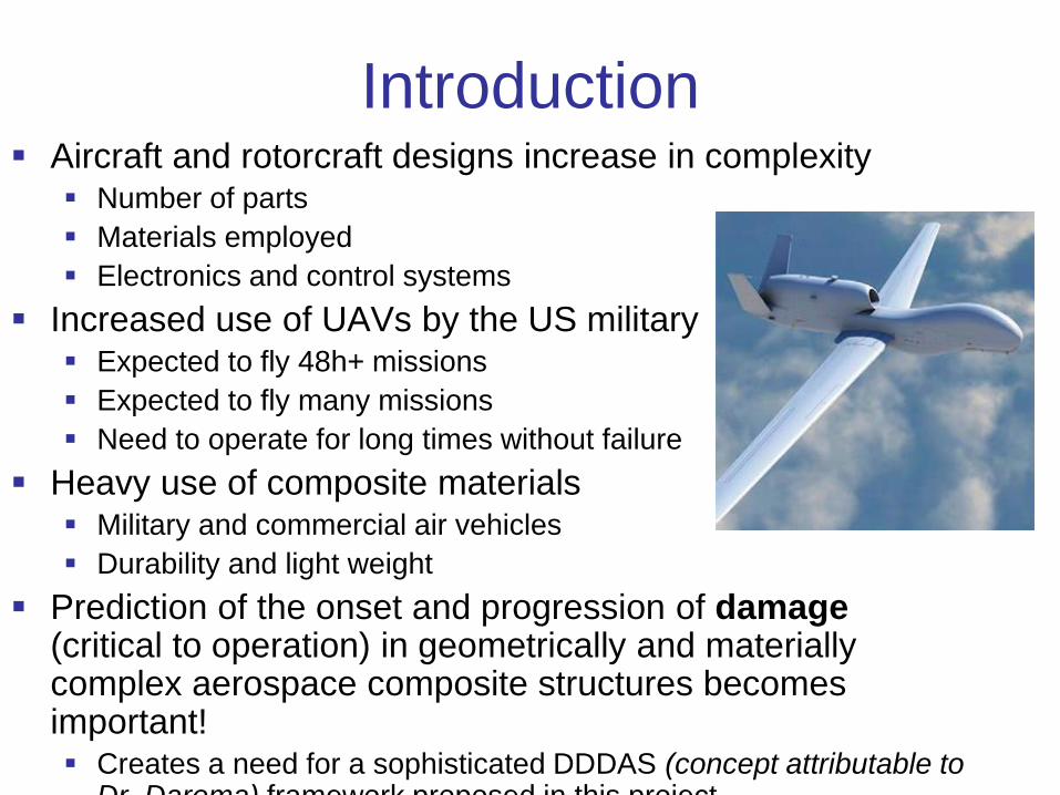
Introduction Aircraft and rotorcraft designs increase in complexity

Number of parts

Materials employed

Electronics and control systems

Increased use of UAVs by the US military Expected to fly 48h+ missions

Expected to fly many missions

Need to operate for long times without failure

Heavy use of composite materials Military and commercial air vehicles

Durability and light weight

Prediction of the onset and progression of damage (critical to operation) in geometrically and materially complex aerospace composite structures becomes important! Creates a need for a sophisticated DDDAS (concept attributable to

Dr. Darema) framework proposed in this project

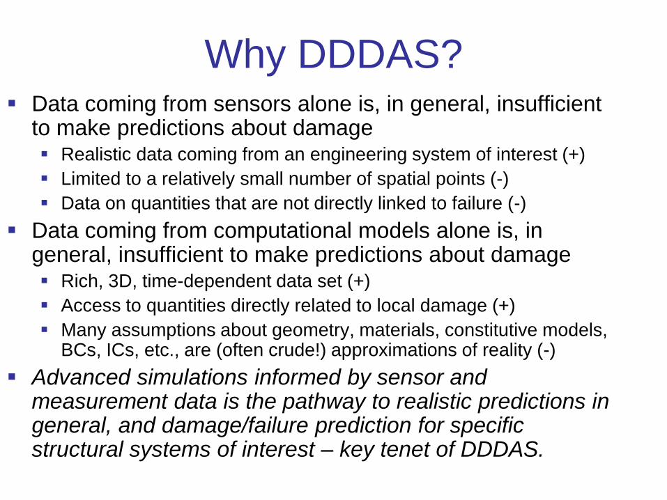
Why DDDAS? Data coming from sensors alone is, in general, insufficient

to make predictions about damage Realistic data coming from an engineering system of interest (+)

Limited to a relatively small number of spatial points (-)

Data on quantities that are not directly linked to failure (-)

Data coming from computational models alone is, in general, insufficient to make predictions about damage Rich, 3D, time-dependent data set (+)

Access to quantities directly related to local damage (+)

Many assumptions about geometry, materials, constitutive models, BCs, ICs, etc., are (often crude!) approximations of reality (-)

Advanced simulations informed by sensor and measurement data is the pathway to realistic predictions in general, and damage/failure prediction for specific structural systems of interest – key tenet of DDDAS.

Methodology:

Advanced modeling and simulation

Time-dependent, 3D complex geometry, non-linear

material behavior

Progressive and fatigue damage modeling in

composite materials

High-fidelity data outputs (stress and damage field

distributions)

Isogeometric Analysis (IGA) for structural mechanics

Efficiency, robustness and suitability for DDDAS

A full-scale 3D composite blade structure with built-in

structural defects

Verification and validation

Instrumented with ultrasonic sensor arrays, infrared

thermographic imaging, accelerometers, strain gauges.

Deployment of the DDDAS framework

Fatigue damage prediction using DDDAS

FSI modeling with nonmatching interfaces

Flexibility

Control using adjoint-based methods

GPU/OpenMP implementation for increased performance

Trailing Edge Adhesive Disbond (4” long disbond)

Shear web to Skin Adhesive Disbond (set of 3 different sizes, 0.5”, 1” and 2” diameter)

Skin to core delamination (set of 3 different sizes, 0.5”, 1” and 2” diameter)

Out-of-Plane Waviness (2 locations, same length, different thickness of waviness)

Trailing Edge Cracks (2-3” perpendicular from trailing edge)

In-plane Waviness (size unknown)

Resin Starved (size unknown)

1/2-thickness

Skin delamination (set of 3 different sizes, 0.5”, 1” and 2” diameter, at different depths)

Full thicknessBoxes not representative of actual size, only define approximate location

3 sizes Ø: 0.5, 1, 2”

IGA, Full-Scale Blade Structure,

Basic Model Validation, and DDDAS

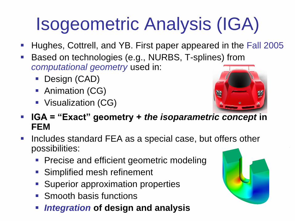
Isogeometric Analysis (IGA) Hughes, Cottrell, and YB. First paper appeared in the Fall 2005

Based on technologies (e.g., NURBS, T-splines) from computational geometry used in:

Design (CAD)

Animation (CG)

Visualization (CG)

IGA = “Exact” geometry + the isoparametric concept in FEM

Includes standard FEA as a special case, but offers other possibilities:

Precise and efficient geometric modeling

Simplified mesh refinement

Superior approximation properties

Smooth basis functions

Integration of design and analysis

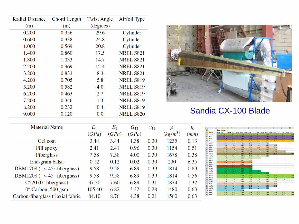
Sandia CX-100 Blade

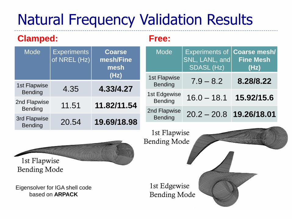
Natural Frequency Validation Results

Mode Experiments

of NREL (Hz)

Coarse

mesh/Fine

mesh

(Hz)

1st Flapwise

Bending 4.35 4.33/4.27

2nd Flapwise

Bending 11.51 11.82/11.54

3rd Flapwise

Bending 20.54 19.69/18.98

Mode Experiments of

SNL, LANL, and

SDASL (Hz)

Coarse mesh/

Fine Mesh

(Hz)

1st Flapwise

Bending 7.9 – 8.2 8.28/8.22

1st Edgewise

Bending 16.0 – 18.1 15.92/15.6

2nd Flapwise

Bending 20.2 – 20.8 19.26/18.01

Clamped: Free:

1st Flapwise

Bending Mode

1st Flapwise

Bending Mode

1st Edgewise

Bending Mode Eigensolver for IGA shell code

based on ARPACK

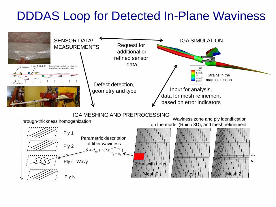
DDDAS Loop for Detected In-Plane Waviness

Ply 1

Ply 2

Ply i - Wavy

Ply N

…

…

Through-thickness homogenization

Mesh 0 Mesh 1 Mesh 2

dev sin(2u u1

u2 u1

)

u1

u2

Parametric description

of fiber waviness

Waviness zone and ply identification

on the model (Rhino 3D), and mesh refinement

Trailing Edge Adhesive Disbond (4” long disbond)

Shear web to Skin Adhesive Disbond (set of 3 different sizes, 0.5”, 1” and 2” diameter)

Skin to core delamination (set of 3 different sizes, 0.5”, 1” and 2” diameter)

Out-of-Plane Waviness (2 locations, same length, different thickness of waviness)

Trailing Edge Cracks (2-3” perpendicular from trailing edge)

In-plane Waviness (size unknown)

Resin Starved (size unknown)

1/2-thickness

Skin delamination (set of 3 different sizes, 0.5”, 1” and 2” diameter, at different depths)

Full thicknessBoxes not representative of actual size, only define approximate location

3 sizes Ø: 0.5, 1, 2”

SENSOR DATA/

MEASUREMENTS

IGA MESHING AND PREPROCESSING

IGA SIMULATION

Defect detection,

geometry and type

Zone with defect

Strains in the

matrix direction

Input for analysis,

data for mesh refinement

based on error indicators

Request for

additional or

refined sensor

data

Modeling of Damage in Large-Scale

Composite Structures: Progressive and Fatigue Damage Modeling

Damage in Composite Lamina & Laminates

Four failure modes considered here: • Fiber rupture in

longitudinal tension;

• Fiber buckling and kinking in longitudinal compression;

• Matrix cracking under in-plane transverse tension and shear;

• Matrix crushing under in-plane transverse compression and shear.

Failure modes of Composites (Courtesy of P. Camannho et al.)

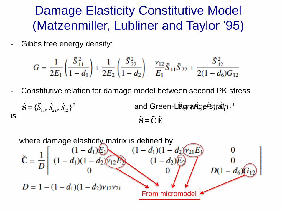
Damage Elasticity Constitutive Model

(Matzenmiller, Lubliner and Taylor ’95)

- Gibbs free energy density:

- Constitutive relation for damage model between second PK stress

and Green-Lagrange strain is

where damage elasticity matrix is defined by From micromodel

S = {S11, S22, S12}T

E = {E11, E22, E12}T

S =CE

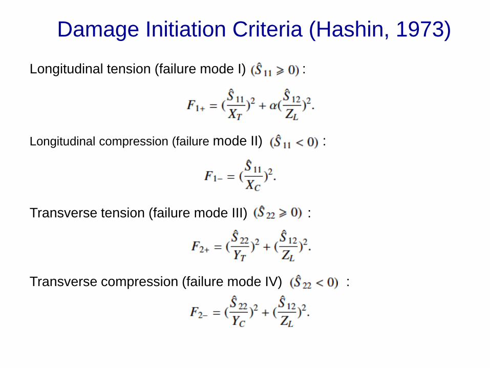
Damage Initiation Criteria (Hashin, 1973)

Longitudinal tension (failure mode I) :

Longitudinal compression (failure mode II) :

Transverse tension (failure mode III) :

Transverse compression (failure mode IV) :

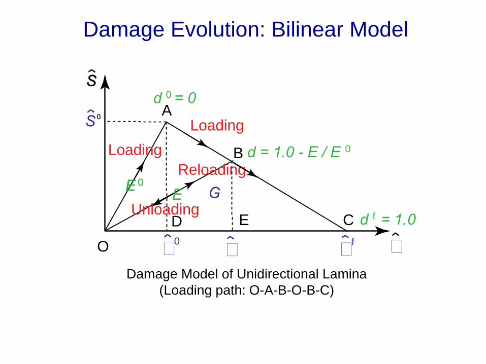
Damage Evolution: Bilinear Model

Damage Model of Unidirectional Lamina

(Loading path: O-A-B-O-B-C)

δ

Loading

Unloading

Loading

Reloading

O

A

B

C

S

0EE

0d = 0

fd = 1.0

0d = 1.0 - E / E

G 0E

0δ

fδ

δ

ED

0

S

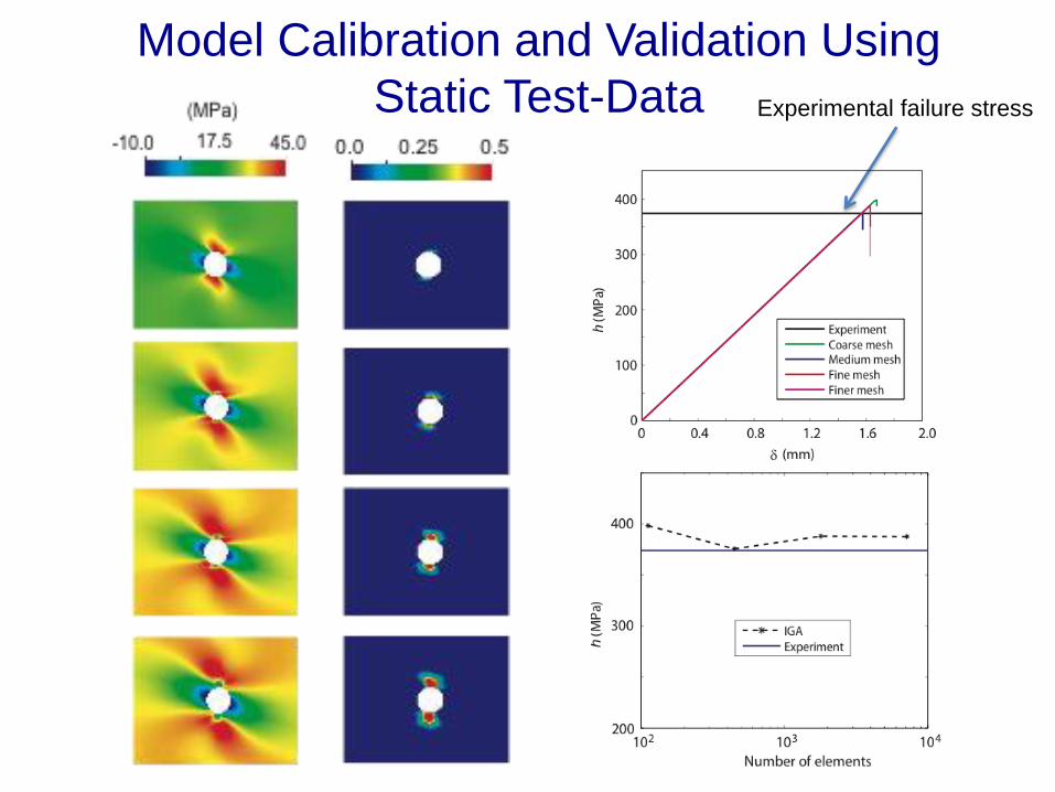
Experimental failure stress

Model Calibration and Validation Using

Static Test-Data

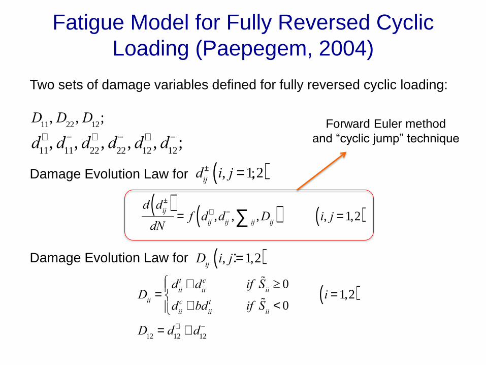
Two sets of damage variables defined for fully reversed cyclic loading:

Damage Evolution Law for :

Damage Evolution Law for :

d dij

±( )dN

= f dij

+ ,dij

- ,ij, D

ijå( ) i, j = 1,2( )

d

ij

± i, j = 1,2( )

D

iji, j = 1,2( )

Dii

=d

ii

t + dii

c

dii

c + bdii

t

ìíï

îï

if Sii³ 0

if Sii

< 0i = 1,2( )

D12

= d12

+ + d12

-

d

11

+ , d11

- , d22

+ , d22

- , d12

+ , d12

- ; D

11, D

22, D

12;

Fatigue Model for Fully Reversed Cyclic

Loading (Paepegem, 2004)

Forward Euler method

and “cyclic jump” technique

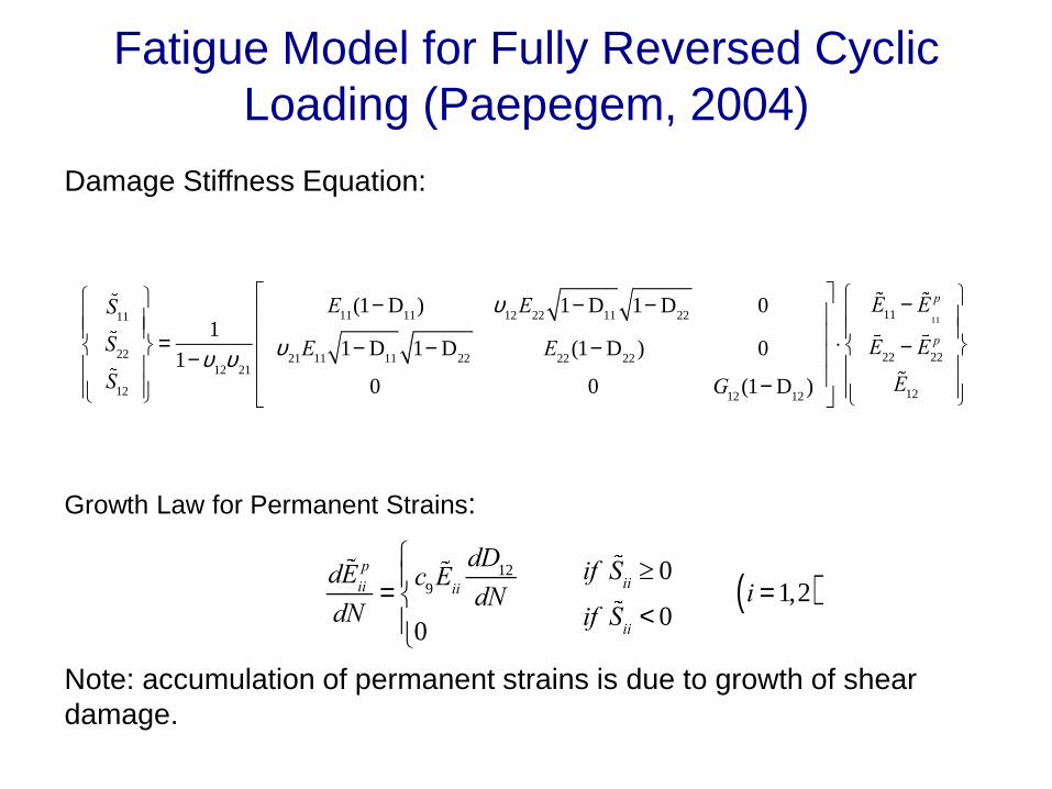
Damage Stiffness Equation:

Growth Law for Permanent Strains:

Note: accumulation of permanent strains is due to growth of shear

damage.

dEii

p

dN=

c9E

ii

dD12

dN

0

ì

íï

îï

if Sii³ 0

if Sii

< 0i = 1,2( )

S11

S22

S12

ì

í

ïï

î

ïï

ü

ý

ïï

þ

ïï

=1

1-u12u

21

E11

(1- D11

) u12

E22

1- D11

1- D22

0

u21

E11

1- D11

1- D22

E22

(1- D22

) 0

0 0 G12

(1- D12

)

é

ë

êêêê

ù

û

úúúú

×

E11

- E11

p

E22

- E22

p

E12

ì

í

ïï

î

ïï

ü

ý

ïï

þ

ïï

Fatigue Model for Fully Reversed Cyclic

Loading (Paepegem, 2004)

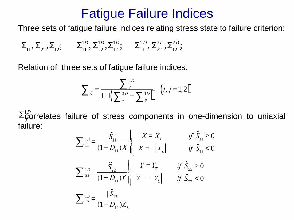
Fatigue Failure Indices Three sets of fatigue failure indices relating stress state to failure criterion:

Relation of three sets of fatigue failure indices:

correlates failure of stress components in one-dimension to uniaxial

failure:

ijå =ij

2 Då1+

ij

2Då -ij

1Då( )i, j = 1,2( )

S

11, S

22,S

12;

S

11

1D , S22

1D ,S12

1D; S

11

2D , S22

2D ,S12

2D;

11

1D =S

11

(1- D11

)Xå

X = XT

X = - XC

ì

íï

îï

if S11³ 0

if S11

< 0

22

1D =S

22

(1- D11

)Yå

Y = YT

Y = - YC

ì

íï

îï

if S22³ 0

if S22

< 0

12

1D =| S

12|

(1- D12

)ZL

å

S

ij

1D

correlates stress components in two-dimensional case to Tsai-Wu in-

plane failure surface:

1

XT

-1

XC

æ

èç

ö

ø÷

S11

11

2 D (1- D11

)å+

1

YT

-1

YC

æ

èç

ö

ø÷

S22

1- D22

+1

XT

XC

S11

11

2 D (1- D11

)å

æ

èç

ö

ø÷

2

+1

YT

YC

S11

1- D22

æ

èç

ö

ø÷

2

+1

ZL

2

S12

1- D12

æ

èç

ö

ø÷

2

= 1

1

XT

-1

XC

æ

èç

ö

ø÷

S11

1- D11

+1

YT

-1

YC

æ

èç

ö

ø÷

S22

22

2 D (1- D22

)å+

1

XT

XC

S11

1- D11

æ

èç

ö

ø÷

2

+1

YT

YC

S22

22

2 D (1- D22

)å

æ

èç

ö

ø÷

2

+1

ZL

2

S12

1- D12

æ

èç

ö

ø÷

2

= 1

1

XT

-1

XC

æ

èç

ö

ø÷

S11

1- D11

+1

YT

-1

YC

æ

èç

ö

ø÷

S22

1- D22

+1

XT

XC

S11

1- D11

æ

èç

ö

ø÷

2

+1

YT

YC

S22

1- D22

æ

èç

ö

ø÷

2

+1

ZL

2

S12

12

2 D (1- D12

)å

æ

èç

ö

ø÷

2

= 1

S

ij

2 D

Fatigue Failure Indices

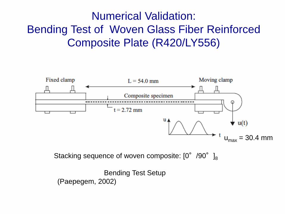
Numerical Validation:

Bending Test of Woven Glass Fiber Reinforced

Composite Plate (R420/LY556)

Stacking sequence of woven composite: [0°/90°]8

Bending Test Setup

(Paepegem, 2002)

umax = 30.4 mm

Material Properties of Woven Composite Lamina

E11

(GPa)

E22

(GPa) ν12

G12

(GPa)

24.57 23.94 0.153 4.83

Measured in-plane elastic properties of

woven composite lamina [0°/90°]

Xt

(MPa)

Xc

(MPa)

Yt

(MPa)

Yc

(MPa)

ZL

(Mpa)

390.7 345.1 390.7 345.1 100.6

Measured in-plane static strengths of

woven composite lamina [0°/90°]

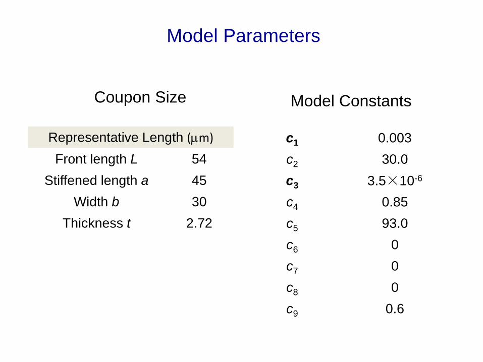
Model Parameters

Coupon Size

Representative Length (mm)

Front length L 54

Stiffened length a 45

Width b 30

Thickness t 2.72

Model Constants

c1 0.003

c2 30.0

c3 3.5×10-6

c4 0.85

c5 93.0

c6 0

c7 0

c8 0

c9 0.6

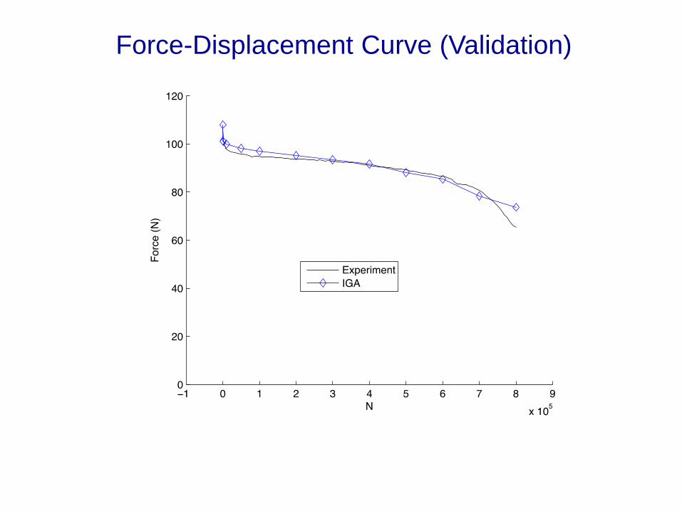
Force-Displacement Curve (Validation)

DDDAS for Full-Scale Blade Fatigue Test (work with Drs. Stuart Taylor (LANL) and

Michael Todd (UCSD), fatigue experiment done at NREL)

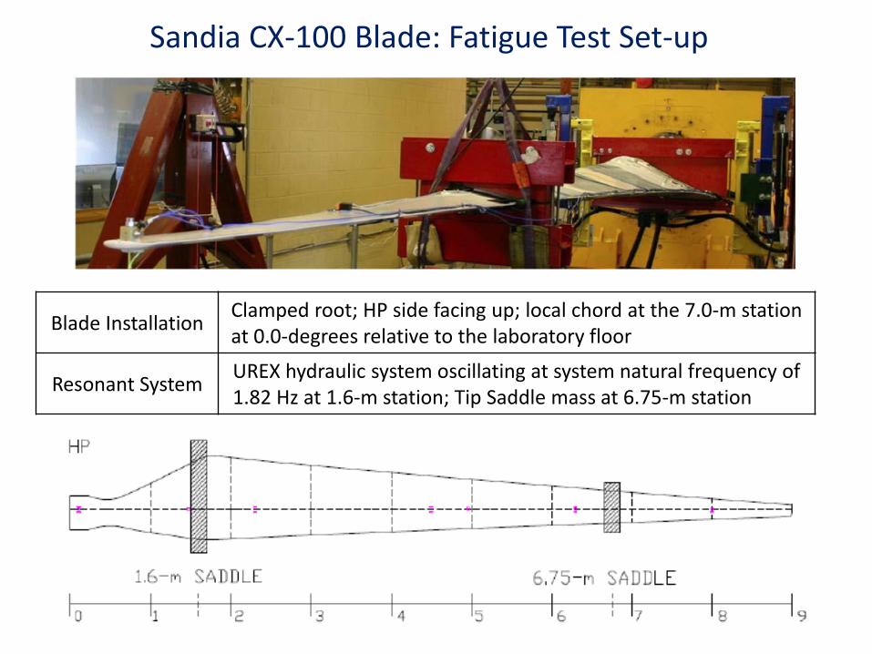
Sandia CX-100 Blade: Fatigue Test Set-up

Blade Installation Clamped root; HP side facing up; local chord at the 7.0-m station at 0.0-degrees relative to the laboratory floor

Resonant System UREX hydraulic system oscillating at system natural frequency of 1.82 Hz at 1.6-m station; Tip Saddle mass at 6.75-m station

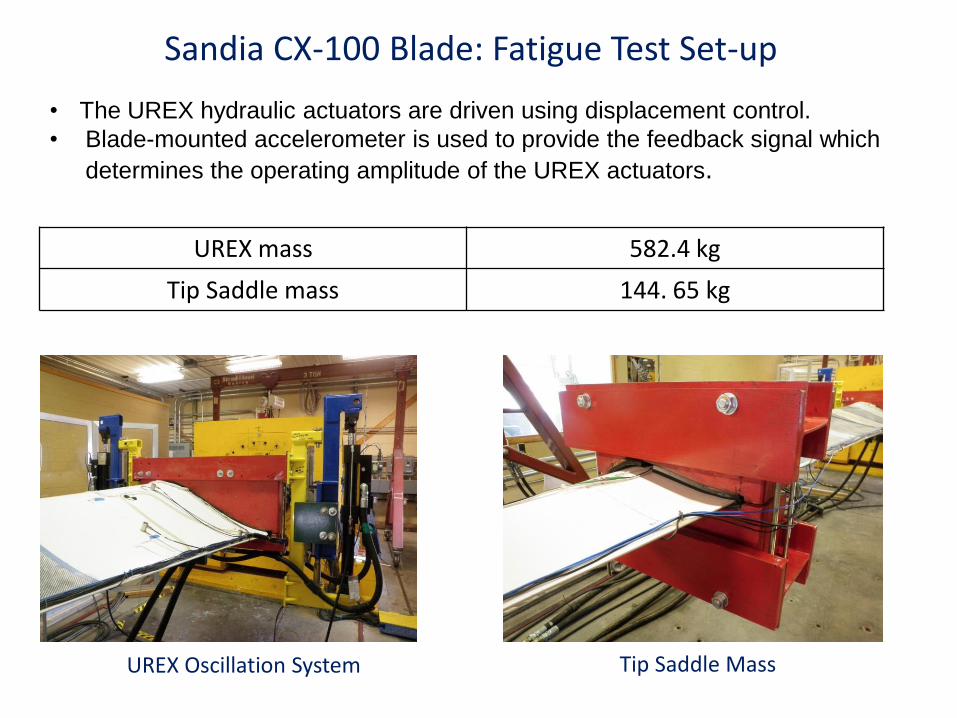
UREX Oscillation System Tip Saddle Mass

UREX mass 582.4 kg

Tip Saddle mass 144. 65 kg

• The UREX hydraulic actuators are driven using displacement control.

• Blade-mounted accelerometer is used to provide the feedback signal which

determines the operating amplitude of the UREX actuators.

Sandia CX-100 Blade: Fatigue Test Set-up

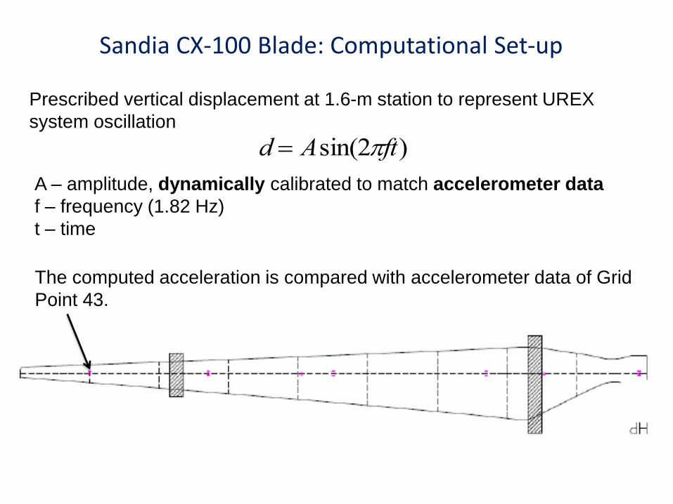
Sandia CX-100 Blade: Computational Set-up

d Asin(2ft)

Prescribed vertical displacement at 1.6-m station to represent UREX

system oscillation

A – amplitude, dynamically calibrated to match accelerometer data

f – frequency (1.82 Hz)

t – time

The computed acceleration is compared with accelerometer data of Grid

Point 43.

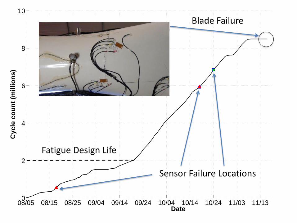
08/05 08/15 08/25 09/04 09/14 09/24 10/04 10/14 10/24 11/03 11/13 08/05 08/150

2

4

6

8

10

Date

Cy

cle

co

un

t (m

illio

ns

)

Sensor Failure Locations

Blade Failure

Fatigue Design Life

Artem’s Movie

Outlook: DDDAS in the Presence of Fluid-

Structure Interaction

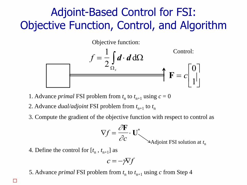
F c0

1

f 1

2d d

s

d

Objective function:

Control:

1. Advance primal FSI problem from tn to tn+1 using c = 0

2. Advance dual/adjoint FSI problem from tn+1 to tn

3. Compute the gradient of the objective function with respect to control as

f F

cU*

Adjoint FSI solution at tn

4. Define the control for [tn , tn+1] as

c f

5. Advance primal FSI problem from tn to tn+1 using c from Step 4

Adjoint-Based Control for FSI: Objective Function, Control, and Algorithm

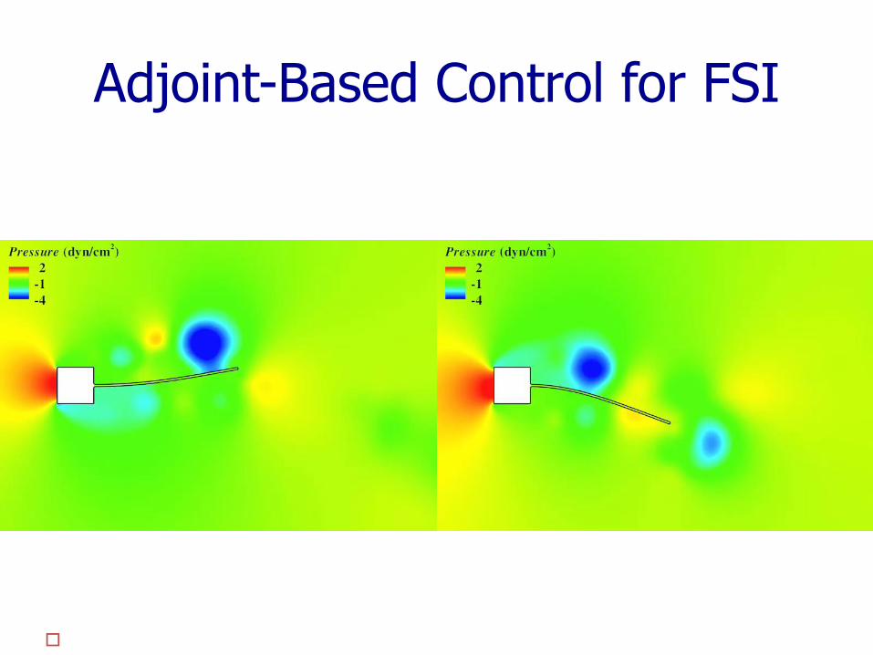
Adjoint-Based Control for FSI

Acknowledgements

AFOSR Award FA9550-12-1-0005, Dr. Frederica

Darema, award monitor

HPC resources provided by TACC and SDSC

Thank You!!!