A data collection and processing procedure for evaluating a

PACIFIC SOUTHWEST Forest and RangeExperiment Station

FOREST SERVICE

U. S. DEPARTMENT OF AGRICULTURE P.O. BOX 245, BERKELEY, CALIFORNIA

A DATA COLLECTION AND PROCESSING PROCEDURE for evaluating a research program

Giuseppe Rensi H. Dean Claxton

USDA FOREST SERVICE RESEARCH PAPER PSW- 81 /1972

CONTENTS Page

Introduction . . . . . . . . . . . . . . . . . . . . . . . . . . . . . . . . . . . . . . . . . . . . . . . . . 1

Input Data . . . . . . . . . . . . . . . . . . . . . . . . . . . . . . . . . . . . . . . . . . . . . . . . . . 2

Data Collection . . . . . . . . . . . . . . . . . . . . . . . . . . . . . . . . . . . . . . . . . . . 2

Data Formatting . . . . . . . . . . . . . . . . . . . . . . . . . . . . . . . . . . . . . . . . . . . 4

Matrix Generation . . . . . . . . . . . . . . . . . . . . . . . . . . . . . . . . . . . . . . . . . . . 6

Input and Generated Data Report . . . . . . . . . . . . . . . . . . . . . . . . . . . . . 7

Project Reports . . . . . . . . . . . . . . . . . . . . . . . . . . . . . . . . . . . . . . . . . . . 7

Organization Report . . . . . . . . . . . . . . . . . . . . . . . . . . . . . . . . . . . . . . . 7

Summary Tables . . . . . . . . . . . . . . . . . . . . . . . . . . . . . . . . . . . . . . . . . . 7

Zero-One Optimization . . . . . . . . . . . . . . . . . . . . . . . . . . . . . . . . . . . . . . 7

Analysis Reports Using Optimization . . . . . . . . . . . . . . . . . . . . . . . . . 8

Summary . . . . . . . . . . . . . . . . . . . . . . . . . . . . . . . . . . . . . . . . . . . . . . . . . . . 9

Appendixes . . . . . . . . . . . . . . . . . . . . . . . . . . . . . . . . . . . . . . . . . . . . . . . . 10

A—Examples of Data Collection . . . . . . . . . . . . . . . . . . . . . . . . . . 10

B—Operating Instructions for Program FILE . . . . . . . . . . . . . . . 14

C—Operating Instructions for Program ZERONE . . . . . . . . . . . 17

FOREWORD

Evaluating proposals for inclusion in a research program is an important, continuing, and difficult decision process for the research administrator. He usually decides on the basis of intuition and experience. Typically, only a small amount of data and analysis are available to him before proposals are selected and molded into a research program.

Recognizing the potential for improving this process, the consistency and perhaps the quality of the decisions, the Forest Service started both theoretical and empirical studies in 1967. Theoretical work was done at the Pacific Southwest Forest and Range Experiment Station in cooperation with the University of California, Berkeley. The U.S. Forest Products Laboratory at Madison, Wisconsin, cooperated by providing data for both theoretical and practical work.

The procedures reported in this paper were developed by the Station in cooperation with the University of California, Berkeley.

The Authors

GIUSEPPE RENSI is a research assistant in the Department of Agricultural Economics, University of California, Berkeley. He is working with the Station in accordance with a cooperative agreement, and was a member of the Station's research staff from 1967 to 1968. He is a graduate in agricultural science of the Facoltá di Agraria, Piacenza, Italy (1961), and holds a master's degree in statistics (1966) and a doctorate in agricultural economics (1968) from the University of California, Berkeley. H. DEAN CLAXTON is in charge of the Station's research on timber conversion systems, with headquarters in Berkeley. He earned a bachelor's degree in economics at Oklahoma State University (1955), a master of forestry degree at Duke University (1958), and a doctorate in agricultural economics at the University of California, Berkeley, in 1968. He joined the Forest Service and the Station staff in 1961.

D ecisions concerning the choice of research projects have historically been based mostly on the intuition, knowledge, and wisdom of the

administrator responsible for deciding. The complex nature of these decisions is readily recognized, but the traditional tools for reducing complex decisions, including the collection and analysis of data, are rarely applied to the problem.

With increasing public awareness of research costs and potential gains from research results, the need for greater internal consistency and rational planning is becoming more apparent than ever before. Increasing availability of large-scale data storage and processing equipment offers an opportunity to improve consistency and rationality in the research planning process.

In recognition of these needs and capabilities, the Forest Service started a series of special studies of the problem. A considerable amount of theoretical and empirical work was carried out to develop an analytical procedure for evaluating and planning research programs in the context of a government research organization. This analytical procedure is based on a descriptive model of a research organization. The definitions and assumptions underlying the model are found in a companion report An Analytical Pro-cedure to Assist Decision-Making in a Government Research Organization, by H. Dean Claxton and Giuseppe Rensi, published by the Pacific Southwest Forest and Range Experiment Station, Berkeley, California, as USDA Forest Service Research Paper PSW-80.

The analytical procedure developed can be most useful when coupled with computer programs or techniques for data storage and manipulation. It could not possibly be used without computer implementation.

This report describes a set of computer programs and subroutines that will partially fulfill the information processing requirements of this analytical procedure.

The over-all cycle of information gathering, processing, and utilization–as specified by the procedure–consists of these five steps:

1. Specification of the relevant data. 2. Assembly and storage of information. 3. Periodical updating of information. 4. Cross-checking of information. 5. Conversion of information into a form usable

for decision-making purposes. The programs documented in this paper were

developed to carry out data manipulations required in steps 2, 3, and 5. From a functional viewpoint, the operations performed in the three steps can be summarized as follows:

I Input data II Matrix generation III Input and generated data report IV Zero-one integer programing optimization V Analysis reports using optimization.

Operation I involves coding and formatting information about the research activity in a form acceptable to data processing media.

Operations II and III produce a schematic description of the status of a research organization at a given time, including: (1) Definition and measurement of performance criteria; (2) definition and measurement of limiting factors; and (3) definition and numerical description of research projects.

In operations IV and V, a zero-one integer programing algorithm uses the information matrix produced in operation II to obtain an optimum set of binary decisions concerning each potential research activity. A "yes" decision on a research project may be interpreted as a recommendation that the project be carried out in the next planning period; the opposite holds for a "no" decision. Operation V, in particular, provides options to use the optimization routine in a repetitive fashion to analyze the sensitivity of optimum decisions to variations in any of the parameters of the problem. Simulated responses to a variety of policy decisions can be thereby explored.

The programs and routines described in this paper do not account for all the information processing tasks required in the analytical approach to research

1

evaluation and planning. Some of the steps in that approach, for example, "cross-checking of the in-formation," do not lend themselves to automated execution. Therefore, these computer programs do not form an integrated, self-contained research plan-

ning software package. More accurately the software elements described here can be considered a means to utilize automated processing facilities in those phases of research planning that require routine manipulations of large amounts of data.

INPUT DATA

Information is assembled and structured in a format appropriate for automated processing. Two steps are involved: data collection and data formatting.

Data Collection The collection of data is done by means of three

reference lists and an appropriately designed data sheet. One such data sheet is used for each proposed research project.

Reference List 1 assigns to each research project in the organization (a) an identification code number; and (b) a title. The identification code is chosen among the numbers ranging from 1 through 999. Different projects should be assigned different code numbers. Different versions of the same research project corresponding to diverse levels of resource outlays and utility contributions should be assigned different code numbers and documented on separate project data sheets.

Reference List 2 contains a set of resources other than budget funds which are available in limited short-run supply to the research organization. The use of these resources is shared by the projects which require them. Examples of such resources may be laboratory space, computing facilities, and personnel with special skills. For each resource entered, Reference List 2 specifies (a) an identification code number; (b) a description of the resource; and (c) a unit of measure for the resource's use.

Reference List 3 specifies a set of achievement criteria other than dollar benefits. For every performance criterion entered, Reference List 3 indicates (a) an identification code number; (b) a description of the performance criterion; and (c) a unit of measure of such performance criterion. Examples of performance criteria other than dollar benefits may be air pollution abatement, and low cost housing.

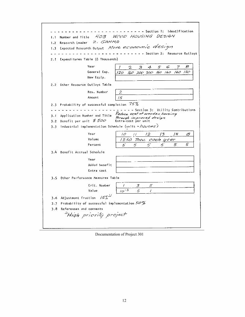
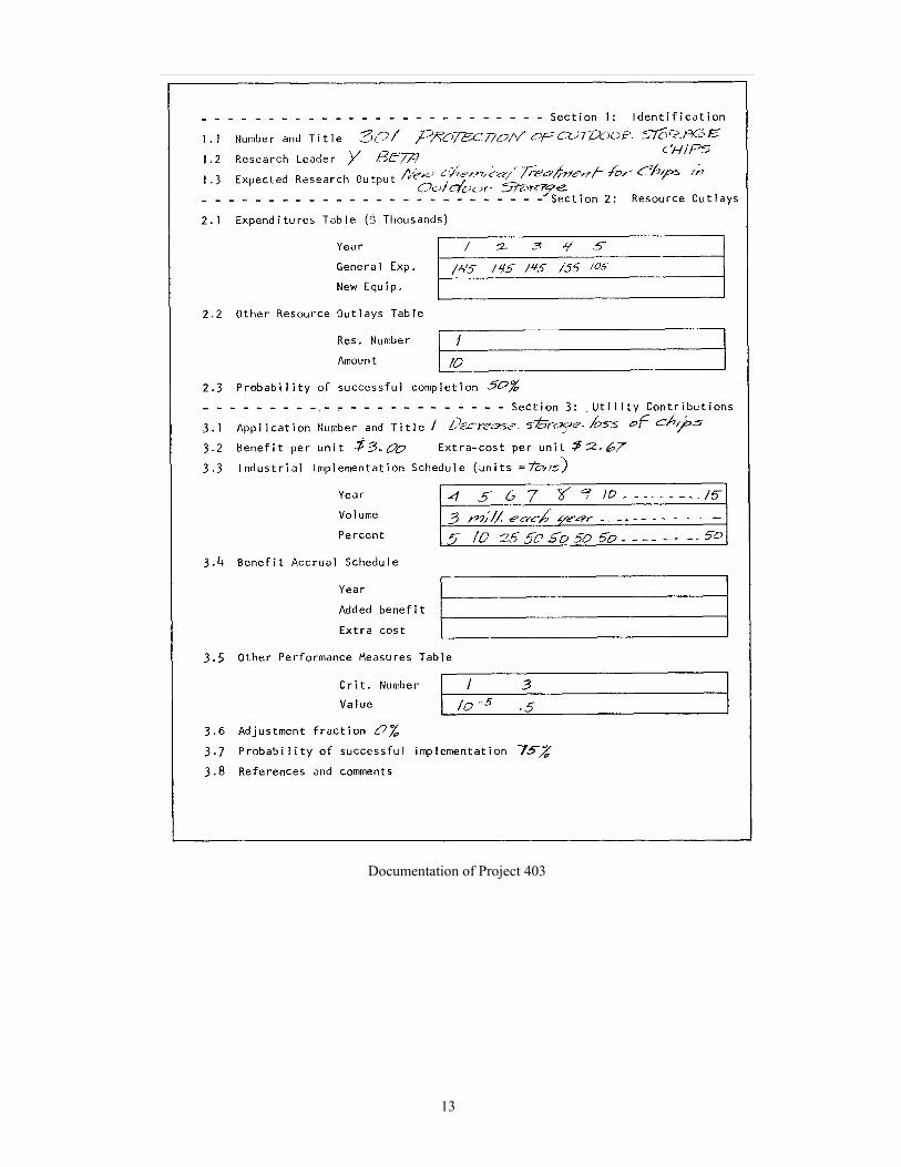
A project data sheet consists of three sections: (1) project identification items; (2) project resource outlays, namely, money expenditures and other

limited resources use; (3) expected utility contributions, namely, economic benefits and other performance measures. 1. Section One: Identification

1.1 Identification Number and Title For the identification code number, consult Reference List 1.

1.2 Research Leader Name of the researcher in charge of the project.

1.3 Expected Research Output. This item refers to the "research phase" of the project. The research phase may be followed by an "implementation phase," i.e., the conversion of research results into socio-economically useful applications. The implementation phase may or may not be carried out by the research organization. Only when the implementation phase is part of the research project do expected research output (item 1.3) and application (item 3.1) coincide. This can happen when a project involves technology development, or research extension. If a project deals exclusively with surveys, classifications, testing of hypotheses, or formulations or verifications of theories, then item 1.3 and 3.1 do not coincide.

2. Section Two: Resource Outlays 2.1 Expenditure Table

–Year –General Expenditures –New Equipment Expenditures

Number the years from 1 through T; T is the project's expected duration, measured in years. General expenditures include salaries, overhead, and current operating expenses. New equipment expenditures refer to procurement costs for equipment required exclusively by the project. Such is the case, for instance, when the project involves equipment development. Yearly

2

cash flows should be recorded to describe the type of transaction planned, e.g., lump payment, installment payments, rentals.

2.2 Other Resource Outlays Table –Resource Number –Amount Required

Resource number indicates the identification code assigned in Reference List 2. Amounts used are measured in the units established in Reference List 2.

2.3 Probability of Successful Completion This item expresses in percent the likelihood that the expected research output entered into 1.3 is achieved within the time and with the resources specified in 2.1 and 2.2.

3. Section Three: Utility Contributions 3.1 Application Number and Title

Applications are consequences of research which have measurable public value. When several applications are listed under the same project use sequential numbers starting from 1.

3.2 Benefit and Extra Cost per Unit Items 3.2 through 3.4 apply when the value of the application examined has an economic dimension, i.e., can be expressed in dollar terms. Such is the case for most technological changes, i.e., product or process innovations. Benefit Or unit expresses, in dollar units, the gross (net) added value per unit of product in a product innovation or the gross (net) cost saving per unit of production in a process innovation. If the net figure is entered, do not record extra cost per unit. If gross benefit per unit is reported, then extra cost per unit must be entered as well. Extra cost per unit measures the unit cost increase required to achieve the gross benefits per unit stated. In process innovations, cost savings in some phases of the production process may be accompanied, and partially offset by cost increases in other phases.

3.3 Industrial Implementation Schedule –Year –Volume –Percent Affected

This table describes the time path of diffusion of the innovation described in item 3.1. Years are counted to begin from the project's inception point, e.g., year t indicates the t-th year since the project

started. Volume equals total production in a given year. Percent affected estimates the fraction of total production affected by the innovation in the same year.

3.4 Benefit Accrual Schedule –Year –Added Benefit –Extra Cost

This item is used instead of item 3.2 and 3.3 when both are not available. If items 3.2 and 3.3 are appropriately filled in, disregard item 3.4. Years are numbered beginning from the project inception. Added benefit and extra cost specify total dollar estimates in a given year. When both added benefit and extra cost arrays are entered, "benefit" indicates gross benefit; when the extra cost row is left empty, "benefit" is interpreted as net benefit.

3.5 Other Performance Measures Table –Criterion Number –Contribution

Criterion number identifies the performance criterion code as specified in Reference List 3. Contribution represents a measure of the project's expected performance according to that criterion. Use the unit measure in Reference List 3.

3.6 Adjustment Fraction The adjustment fraction expresses, in percent, the rate at which the net dollar benefit of the project should be increased (discounted) to take into account desirable (or undesirable) aspects not properly reported under other items. Examples of such aspects may be positive or negative effects on income distribution, positive or negative effects on the quality of the environment not quantified otherwise, or lower priority of the project when similar research is carried out by other individuals or institutions.

3.7 Probability of Successful Implementation This item shows the likelihood, expressed in percent, that the results generated will be converted into useful applications as specified in items 3.1 through 3.5.

3.8 References and Comments Outline the sources of information and assumptions underlying the construction of estimates.

Appendix A illustrates examples of Reference Lists 1, 2, 3, and three project data sheets.

3

Data Formatting Data formatting consists of specifying the format

in which information data sheets are transferred onto punch cards. The sequencing of cards and the information content of each card in the sequence must be indicated. A complete card deck consists of three parts: (1) control cards; (2) project data cards; and (3) organization data cards.

Control Cards Control cards contain instructions concerning the

specification of basic constraints. "Basic" constraints are those constraints whose coefficients may be read directly from project data sheets. The three categories of basic constraints are: (1) Budget constraints; (2) Limited resources constraints; and (3) Performance target constraints.

A card deck sequence is as follows: 1. Basic constraints control card 2. Budget years control card(s) 3. Limited resources control card(s) 4. Performance target control card(s)

The control cards and deck setups outlined above allow a considerable degree of flexibility in the specification of basic constraints and the corresponding interaction with other data cards. Project data cards may contain information about constraints in any of the three categories of basic constraints not being used in the analysis. For example, information may be available on 20 limited resources, but the analyst wants to consider only five as actual constraints. Control cards allow him to disregard information about the remaining 15 constraints without modifying the information base contained in project data cards.

Appendix B details the coding instructions for control cards.

Project Data Cards Information about a single research project is

organized in a sequence of project data cards. The information recorded is the set of coefficients of the basic constraints and the benefit information. Both are taken directly from a project data sheet or constructed from the information on the sheet. Each data block of project data cards is arranged in this card sequence:

1. Project identification card 2. Project parameter card 3. General expenditures card(s) 4. New equipment expenditures card(s)1

5. Limited resources card(s)1

1These cards can be omitted or included depending on instructions in project parameter card. 2These cards can be omitted or included depending on instructions in application parameter card. 3Inclusion or omission of these cards depends on instructionsinput into the basic constraints control card.

6. Limited resources use card(s)1

7. Application title card 8. Application parameter card 9.* Benefit per unit card

10.* Production volume card(s) 11.* Percent acceptance card(s) 12. Performance criteria card(s)2

13. Performance measures card(s)2

If more than one application is documented, card sequence 7 through 13 is repeated for each application. Cards 9*, 10*, 11* are used only when items 3.2 and 3.3 are available in the project data sheet. This condition is called Benefit Documentation Case One. When only item 3.4 is recorded in the project data sheet (called Benefit Documentation Case Two), the starred card sequence is replaced by the sequence:

1. Added benefits card(s) 2. Extra cost card(s).

When only the "added benefit" row of item 3.4 is available in the project data sheet (Benefit Docu-mentation Case Three), the starred card sequence is replaced by:

Net benefit card(s).

Card sequence 1 through 13 has been designed to reflect the structure of the project data sheets.

Detailed coding instructions are in Appendix B.

Organization Data Cards

The organization data cards contain the information necessary to specify constraints of the organization. The bounds or limits on the basic constraints are stated first. The card sequence for basic constraint limits is:

1. Budget level card(s)3

2. Limited resource level card(s)3

3. Performance level card(s).3

Added next is information on "added" constraints, which can be of three types: (1) Allocation constraints; (2) Interdependence constraints; and (3) Miscellaneous constraints. Added constraints can be

4

specified independently of the information found in the project data sheets. The card deck organization is:

Allocation parameter card Allocation project card(s)

Interdependence parameter card Interdependence project card(s)

Miscellaneous parameter card Miscellaneous project card(s) Miscellaneous coefficient card(s)

The order in which the three added constraint types are input is unrestricted. For example, two allocation constraints, three interdependence constraints, and one miscellaneous constraint can be sequenced as follows: M, I, I, A, I, A. Given the added constraint type, however, i.e., A, I, or M, the card succession indicated must be respected. A separation card, i.e., a card with the character "9" punched across columns 1 through 80, must be interposed between project data cards and organization data cards. A termination card, i.e., a card with the character "–" punched across columns 1 through 80 must appear at the end of the complete deck. Detailed instructions as to the information content of each card are given in Appendix B.

To summarize, a complete deck is stacked as follows:

The order in which project data blocks are entered does not matter as long as the cards within a data block are properly ordered. After the information has been transferred to a card deck according to the instructions here specified, it can be processed by means of program FILE and its associated subroutines. In the listing 4 of FILE, input sections pertaining to different card types are carefully enclosed between comment statements. This arrangement makes it expedient for the user to identify the program instructions that affects each card input. Two types of error messages can be produced during the execution of FILE. The first type of error occurs when the maximum number of projects allowed is exceeded or when the maximum number of constraints allowed is exceeded. These maximum limits have been set, tentatively, at 250 projects and 50 constraints. The second type of error consists of improper card sequencing. The corresponding error message reveals which card has been misplaced or assigned an improper identification code.

4A listing of computer programs and subprograms described in this report can be obtained by writing to the Director, Pacific Southwest Forest and Range Experiment Station, P.O. Box 245, Berkeley, California 94701.

5

MATRIX GENERATION

As the data are processed by program FILE a basic information matrix is produced. This matrix represents the essential input for the optimization algorithms that characterize the two operations: Zero-One Optimization and Analysis Reports Using Optimization. The structure of the matrix can be illustrated in this way:

Column 0 of the matrix represents the values Vj; i = 1,...,N, of the projects listed. Columns 1 through M describe the constraints of the organization. For any given project index, a project's value is calculated as

V = po ∑ pj (1 + Wj)Dj - C j≥1

in which po = probability of successful completion pj = probability of implementation of appli

cation j Wj = priority factor for application j Dj = discounted net benefit for application j C = discounted cost of the project The discounted net benefit of any given appli

cation can be expressed as

1T 1D = ∑ z t ( )t

t=1 1+ r

in which zt is the net benefit in the year t, T1 is the last year in which benefits are generated from the application, and r is the rate used in the discount formula. In terms of project data zt is calculated in different ways, depending on the Benefit Documentation Case encountered. For Case One z t is calculated as the product of net unit benefit times volume in year t times percent affected in year t. In Case Two, zt is computed as the difference between added benefit and extra cost in year t. In Case Three, zt equals net benefit in year t as originally input.

The discounted research cost of the project (C) is

TC = ∑ c t ( 1 )t

t=1 1+ r

in which ct is the project's expenditure in year t, i.e., general expenditures plus new equipment expenditures, and T is the project's duration expressed in years.

A given constraint is specified by these three items: (1) The constraint coefficients a1; i=1, N; (2) the constraint inequality sign; and (3) the constraint bound b. The constraint bound is an upper bound when the inequality sign is "≤" and a lower bound when the inequality sign is "≥" The matrix columns display groups of constraints in this succession from left to right: (1) budget constraints; (2) limited resources constraints; (3) performance target constraints; and (4) added constraints.

For budget constraints, al is the planned research expenditure on project i in a given year and b is the organization's budget in that year. al is calculated by summing general research expenditures and new equipment expenditures for project i. The inequality sign is "≤" For limited resources constraints, aj represents resource consumption by project i and b is the amount of resource available to the organization. The inequality sign is also "≤" In the case of performance target constraints, al measures the performance contribution of project i and b is the minimum performance standard for the organization as a whole. The inequality sign is “≥” the case of added constraints, the definition of aj; i=1,..., N, b and the inequality sign depends on the specific instance of constraint considered. For details on the specification of added constraints see Appendix B.

6

5 Net in this context means net with respect to extra production costs incurred in the application.

INPUT AND GENERATED DATA REPORT The information input as well as data generated by

the program are printed in this order:

1. Project reports 2. Organization report 3. Summary tables.

Project Reports For each research project information package

processed the various data items input are printed out under appropriate titles. The outcome is essentially a computer-produced replicate of the original project data sheet. In addition, the computed net benefit schedule for the project is printed. This output feature can be used in several ways, such as checking for coding or keypunching errors, producing updated reports on the status of research activities, and providing material for updating or cross-checking purposes.

Organization Report The organization report provides a summary of the

number and types of constraints specified as feasibility criteria in the process of research program formulation. Constraints are numbered sequentially 1, 2, ..., etc. and for each number an explanatory title describes the nature of the constraint. The numbering of the constraints is consistent with the column number in the basic information matrix described in the chapter on Matrix Generation.

Summary Tables Three summary tables are produced. Table I

displays a number of intermediate stages in the elaboration of the project benefits, i.e., column zero of the basic information matrix. Table I consists of eight columns of numbers:

1. Project number is a sequential number 1, 2, ..., etc., indicating the listing order.

2. Project identification code number is the code assigned to the project in Reference List 1.

3. Gross benefit is the aggregate present value of net 5 benefits from all the documented applications of a project.

4. Research cost is the present value of planned project expenditures.

5. Net unadjusted benefit is gross benefit minus research cost.

6. U–factor is an estimate of the degree of confidence that the economic results of a project as documented will materialize.

7. EE–factor is an estimate of the adjustment required to account for intangibles, or externalities not sufficiently considered in the documentation of the project.

8. Adjusted net benefit equals unadjusted net benefit multiplied by U–factor and EE–factor. Adjusted net benefit corresponds to the first column of the basic information matrix described in Matrix Generation.

Table II shows a ranking of the projects in terms of benefit over cost ratio. Benefit here is equivalent to adjusted net benefit. Benefit over cost ranking is useful for a quick assessment on the comparative potential performance of the projects. Projects with unusually high or low ratios can be identified easily. Unexpected discrepancies between benefits and costs in certain projects may also alert the investigator to double check the basic data and assumptions put forth in the documentation of these projects.

Table III lists numerical values and inequality indexes for all the constraints described in the organization report. Table III corresponds to the constraint columns, i.e., columns 1 through M of the basic information matrix described in the chapter on Matrix Generation.

ZERO-ONE OPTIMIZATION

The zero-one integer programing method to select an optimum research program consists of identifying a mix of research projects whose sum of benefits is largest among all feasible alternatives. A research program is "feasible" if it is consistent with the organization's constraints. Several computer programs have been developed which identify an optimum

project mix by means of a zero-one integer programing algorithm. These programs have been tested on a UNIVAC 1108 computer. The input required is the basic information matrix described in the chapter

7

on Matrix Generation. The output generated includes: (1) Optimum research program; (2) total benefit associated with the optimum program; and (3) constraint levels corresponding to the optimum program.

In applied mathematics, the computational techniques used belong to the class of branch-and-bound integer programing algorithms. This class ofalgorithms is similar in structure to a tree-search algorithm because it must follow a path along the tree of solutions. Whether the node is terminal or not must be determined at each node of the tree. It is defined as "terminal" when all solutions having that node may be disregarded. This is the case only when all feasible solutions, if any–including the node–are worse off than the current best solution, i.e., the best solution found in prior search. When a terminal node is encountered the search backtracks to the immediately preceding node and embarks on a different path until another terminal node is found. The search is completed when the search process backtracks to the initial node of the tree, and such node is found to be terminal. In general the solution enumeration and record-keeping procedure implicit in this technique is common to most branch-and-bound types of zero-one programing algorithms. What distinguishes algorithms

is the type and sequencing of terminality tests, i.e., tests used to determine whether or not a node is terminal.

In this sense these four programs represent different zero-one integer programing algorithms: (1) Petersen algorithm; (2) revised Petersen algorithm; (3) GR algorithm; and (4) zero-one algorithm with bounded linear programing subroutine. The comparative performance of algorithms 1, 2, and 3, measures, in execution time, varied according to the data used in the test runs. Although the Petersen 6

algorithm requires more iterations to identify an optimum set than do algorithms 2 and 3, its computing time per iteration is less. The revised Petersen algorithm and the GR algorithm perform best when (a) the number of constraints is large in relation to the number of projects or (b) the constraints are tight and as a consequence, there are relative fewer feasible solutions to the optimum project mix problem. Algorithm 4 represents an attempt to implement a computational technique proposed by Geoffrion. 7 The attempt was only partially successful in that an operational program was developed, but further programing work is required to achieve fully the potential efficiency of the technique.

ANALYSIS REPORTS USING OPTIMIZATION Sensitivity analysis based on an optimization

scheme addresses itself to the question of how an optimum solution varies in response to changes in the problem data. In the context of research program formulation and evaluation, sensitivity analysis can be used to explore organization bottlenecks and robustness of optimum decisions.

Bottlenecks in an organization can be investigated by modifying the specification of the organization's constraints. This can be done by adding or deleting constraints as well as by relaxing or strengthening constraints. Comparing optimum sets of projects obtained under, different constraint specifications demonstrates the effect of changes in the constraints. At the same time constraint sensitivity-analysis provides an indication of the potential effectiveness of management policies which can be interpreted as changes in the organization's constraints. For instance, one may explore in a simulated experiment the effects of expanding future budgets by 10 percent on a research program.

Robustness of optimum decisions concerns the

question of how much errors in data affect the computation of optimum project sets. Since subjective judgments and guess work are used in determining a portion of the basic data pertaining to research evaluation and planning, the question is legitimate in this context. An optimum solution is said to be "robust" if it is not drastically affected by error variability in the estimates making up the data base. Robustness determinations can be made in two ways; (1) given a specific change in the optimum solution determine the variation in the data required to produce it; and (2) given a change in the data, determine the induced variation on the optimum set.

Sensitivity analysis in the context of zero-one optimization is performed by the program ZERONE

6 Petersen, Clifford C. Computational experience with vari-ants of the Balas algorithm applied to the selection of R. and D. projects. Manage. Sci. 13(9): 736-750. 1967. 7 Geoffrion, A. M. Implicit enumeration using an imbedded linear program. RAND Corp. RM-5406-PR. 13 o. 1967.

8

and its complementary subprograms. Standard options are provided for these types of analysis:

A: Add, delete. or change an activity or a con-straint.

B: In some specified constraints, change constraint bounds by a fixed additive or multiplicative amount.

C: For all projects listed, determine the amount of error in the estimate of the project benefit necessary to alter the optimum solution with respect to that project.

In ZERONE any sequence of sensitivity analyses can be carried out. The data deck is set up as follows:

1. Control cards 2. Basic tableau cards 3. Sensitivity analysis cards.

The control cards specify the dimensions of the basic tableau as well as the number and sequence of sensitivity analysis options desired. The basic tableau is similar to the basic information matrix described in the chapter on Matrix Generation. It includes project benefits, constraint coefficients, constraint inequality signs, and constraint bounds. Sensitivity analysis cards are required only for options in Type A and Type B. Specific operating instructions for ZERONE are given in Appendix C.

SUMMARY

Rensi, Giuseppe, and H. Dean Claxton. 1972. A data collection and processing procedure for evaluating a

research program. Berkeley, Calif., Pac. Southwest Forest and Range Exp. Stn. 18 p. (USDA Forest Serv. Res. Paper PSW-81)

Oxford: 945.4:U65.012–U681.142. Retrieval Terms: research administration; proposal evaluation; ana-lytical procedures; computer programs; mathematical models.

Evaluating and planning research in an organi-zation usually requires considerable detailed infor-mation. The data needed are concerned with the organization and its objectives and resources and, for each research proposal, the expected contributions to these aims and the requirements for resources.

To detail these information requirements, a data classification scheme was developed. From the scheme, a mechanism for collecting, processing, and analyzing data was devised.

This report provides instructions on how to complete the data collection forms, code the data for transfer to punchcards, and process the data by computer programs. It complements the publication An Analytical Procedure to Assist Decision-Making in a Government Research Organization (USDA Forest Service Research Paper PSW-80).

The set of standardized data collection forms include three reference lists, and project data sheets. Reference list one classifies and identifies the research proposals to be examined; reference list two itemizes the organization's resources; and reference list three

enumerates the organization's objectives. The project data sheets serve the purpose of collecting infor-mation on individual research proposals.

A coding system transfers the information from the data collecting forms to punchcards. This work involves essentially (a) the card deck layout, i.e., the sequence order of cards in the deck; (b) the infor-mation content of each card; and (c) the keypunch configuration for every item on a given card.

A set of computer programs is used to process the information stored on cards. Written in FORTRAN V language, the programs are operational on a UNIVAC 1108 computer. The major tasks that can be per-formed by these programs are: (a) preliminary elab-oration of data, such as calculation of sums, per-centages, discounted values, and benefit-cost ratios; (b) tabular display of data as originally entered as well as in elaborated form; (c) computation of best research activity mix under current organizational constraints; (d) computation of best project mix under alternative conditions, i.e., sensitivity analysis. The computations of (c) and (d) are centered around a zero-one integer programing optimization scheme.

9

APPENDIXES

A—Examples of Data Collection

Reference List 1 Code number

Project description: Polysulphide process 101 Better design in paper production 102 Dry forming 103 Quality of paper products 104 Cost of paper 105 Drying process for oak 201 Pit aspiration in coniferous sapwood 202 Moisture content prediction 203 Eliminate coloring defects 204 Check prevention method 205 Protection of chips in outdoor storage 301 Chemical properties of wood 302 Conversion of wood residues 303 Pollution reduction 304 Tall oil 305 Strength properties of wood elements 401 Interaction of wood elements 402 Techniques for use of wood in housing 403 Particle board, fiberboard design 404 Acoustical performance of wood housing 405 Wood defect detection 501 Wood species identification 502 Nutrient modification 503 Lumber grade mix 504 Sawing methods 505

Reference List 2

Code Unit of number measure

Resource description: Lignin chemists 001 Man years Wood engineers 002 Man years Systems analysts 003 Man years Electronic microscope Type A 004 Hrs. per week Electronic microscope Type B 005 Hrs. per week Computer Type X-next year 006 Hrs. per weekPilot plant space 007 Hrs. per week Laboratory space-next year 008 Sq. ft. Laboratory space-two years

from now 009 Sq. ft. Office space 010 Rooms

Reference List 3

Code number Unit of measure

Criterion description: Increase employment 001 Percentage points Increase proportion of people

above poverty level 002 Percentage points Reduce wood waste in

cutting 003 Million B.F. Reduce sulphur pollution

near paper plants 004 Percentage points Reduce wood waste in

processing 005 Million B.F. Increase amount of wood

products recycled-three years from now 006 Million cu. ft.

Same-five years from now 007 Million cu. ft. Same-ten years from now 008 Million cu. ft.

10

Documentation of Project 101

11


12


13

B—Operating Instructions

for Program FILE

A. General Instructions Coding instructions in Sections B, C, and D that

follow assign a field to each data item entered on a card. A "field" is a set of adjacent columns; for example, columns 1-6 form a six-column field. Except for titles, which can be entered in free format onto the preassigned field, coded data must be "right-oriented" or "right-justified." This require-ment means that any input item is placed in its field in such a way that its right most digit or letter falls into the right most column of the field. For example, the number "521" would be input into columns 43-48 as follows: columns 43-45 empty, "5" into column 46, "2" into column 47 and "1" into column 48.

In all cards, columns 69-80 are reserved for card identification codes:

1. Data package code number: columns 69-72 2. Card type code word: columns 73-76 3. Continuation card number: columns 77-80.

The data package code is "0"–or blank–for control cards and organization data cards. It corre-sponds to the project identification code number for project data cards. Card type code words are listed below in B, C, and D. Continuation card numbers are used to identify continuation cards that follow a given card. "1" identifies the first continuation card, "2" the second, etc.

Sets of information items can be entered onto data cards in two different "patterns": (1) A-pattern or array pattern; or (2) S-pattern or scatter pattern.

A-pattern is used to input arrays of numbers. The first 10 numbers of the array are entered into columns 1-60, one six-column field for each number. If the array contains more than 10 numbers, continu-ation cards are used, in the same fashion, to input the remaining numbers, one continuation card for every additional 10 numbers. Columns 61-66 can be used, if necessary, to enter a scale factor. This factor ex-presses the power of 10 by which the entries in columns 1-60 of the same card must be multiplied for scaling purposes. Numbers must be entered onto card(s) in the same order as they appear in the array.

The S-pattern is used to enter heterogeneous numerical items as well as titles. The order of entry is specified in the following instructions. Unless other-wise indicated, entries are assigned six-column fields– starting with columns 1-6.

B. Instructions for Control Cards

Card 1 Coding 2 Card 3 Entries sequence pattern type

1 S a. Number of budget constraints CCC

b. N umber of resource constraints

c. Nu mber of performance constraints

2 A Budget c onstraint years, as many as indicated in 1.a. If none omit card. YYY

3 A Resour ce code numbers, as many as indicated in 1.b. If none omit card. RRR

4 A Performance criteria numbers, as many as stated in 1.c. If none omit card. TTT

1 See text: Data Formatting–Control Cards.2 See A. General Instructions.3 Card type code word.

C. Instructions or Project Data Cards

Card1 Coding2 Card3

Entries sequence pattern type

1 S a. Project code number IDF b. Descriptive title: cols.

7-68 2 S a. Duration of project in

years PAR b. Probability of comple-

tion–DS 2.34

c. New equipment expend-i t u r e s ? "1 " i f y e s . Blank if none.

d. Nu mber of limited re-sources used. Blank if none.

e. Number of applications. Blank if only one.

3 A General expenditures ($1,000)–second row of DS GEN 2.1

4 A New equipment expendi-tures–third row of DS 2.1. EQP Omit if 2.c is blank.

5 A Resource code numbers–first row of DS 2.2. Omit if 2.d is blank. OLR

6 A Amounts used –second row of DS 2.2. Omit if 2.d is blank. USE

7 S Descriptive title of the application: cols. 1-68 APP

14

Card 1 Coding2 Card3


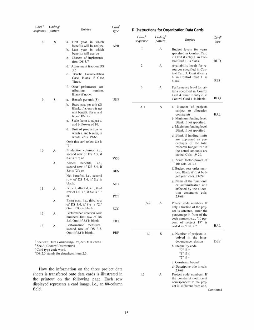
8 S a. First year in which benefits will be realize APR

b. L ast year in which benefits will accrue

c. Chances of implementa-tion–DS 3.7

d. Adjustment fraction DS 3.6

e. Benefit Documentation Case. Blank if Case Three.

f. Other performance con-tributions number. Blank if none.

9 S a. Benefit per unit ($) UNB b. Extra cost per unit ($)

Blank, if a. entry is net unit benefit. For a. and b. see DS 3.2.

c. Scale factor to adjust a. and b. Power of 10.

d. Unit of production to which a. and b. refer, in words, cols. 19-68.

Omit this card unless 8.e is“1”

10 A Production volumes, i.e.,second row of DS 3.3, if 8.e is "1"; or VOL

A Added benefits, i.e., second row of DS 3.4, if 8.e is "2"; or BEN Net benefits, i.e., second row of DS 3.4, if 8.e is blank. NET

11 A Percent affected, i.e., third row of DS 3.3, if 8.e is "1" or PCT

A Extra cost, i.e., third row of DS 3.4, if 8.e s " 2." Omit if 8.e is blank. ECO

12 A Performance criterion code numbers–first row of DS3.5. Omit if 8.f is blank. CRT

13 A Performance measures– second row of DS 3.5. Omit if 8.f is blank. PRF

1 See text: Data Formatting–Project Data cards. 2 See A. General Instructions. 3 Card type code word. 4 DS 2.3 stands for datasheet, item 2.3.

How the information on the three project data sheets is transferred onto data cards is illustrated in the printout on the following page. Each row displayed represents a card image, i.e., an 80-column field.

D. Instructions for Organization Data Cards Card 1 Coding2 Card3


I A Budget le vels for years specified in Control Card 2. Omit if entry a. in Con-trol Card 1. is blank. BUD

2 A Availability levels for resources specified in Con-trol Card 3. Omit if entry b. in Control Card 1. is blank. RES

3 A Perfor mance level for cri-teria specified in Control Card 4. Omit if entry c. in Control Card 1. is blank. REQ

A.1 S a. Number of projects subject to allocation constraints BAL

b. Minimum funding level. Blank if not specified.

c. Maximum funding level. Blank if not specified

d. Blank if funding limits are expressed as per-centages of the total research budget. "1" if the actual amounts are stated. Cols. 19-20.

e. Scale factor–power of 10: cols. 21-22

f. Budget year order num-ber. Blank if first bud-get year: cols. 23-24.

g. Name of the functional or administrative unit affected by the alloca-tion constraint: cols. 25-68

A.2 A Project code numbers. If only a fraction of the proj-ect is affected, enter the percentage in front of the code number, e.g., "10 per-cent of project 19" is coded as "10019." BAL

1.1 S a. Number of projects in-volved in the inter-dependence relation DEP

b. Inequality code: "0" if ≥"1" if ≤"2" if =

c. Constraint bound d. Descriptive title in cols.

25-68 1.2 A Project code numbers. If

the constraint coefficient correspondent to the proj-ect is different from one,

Continued

15

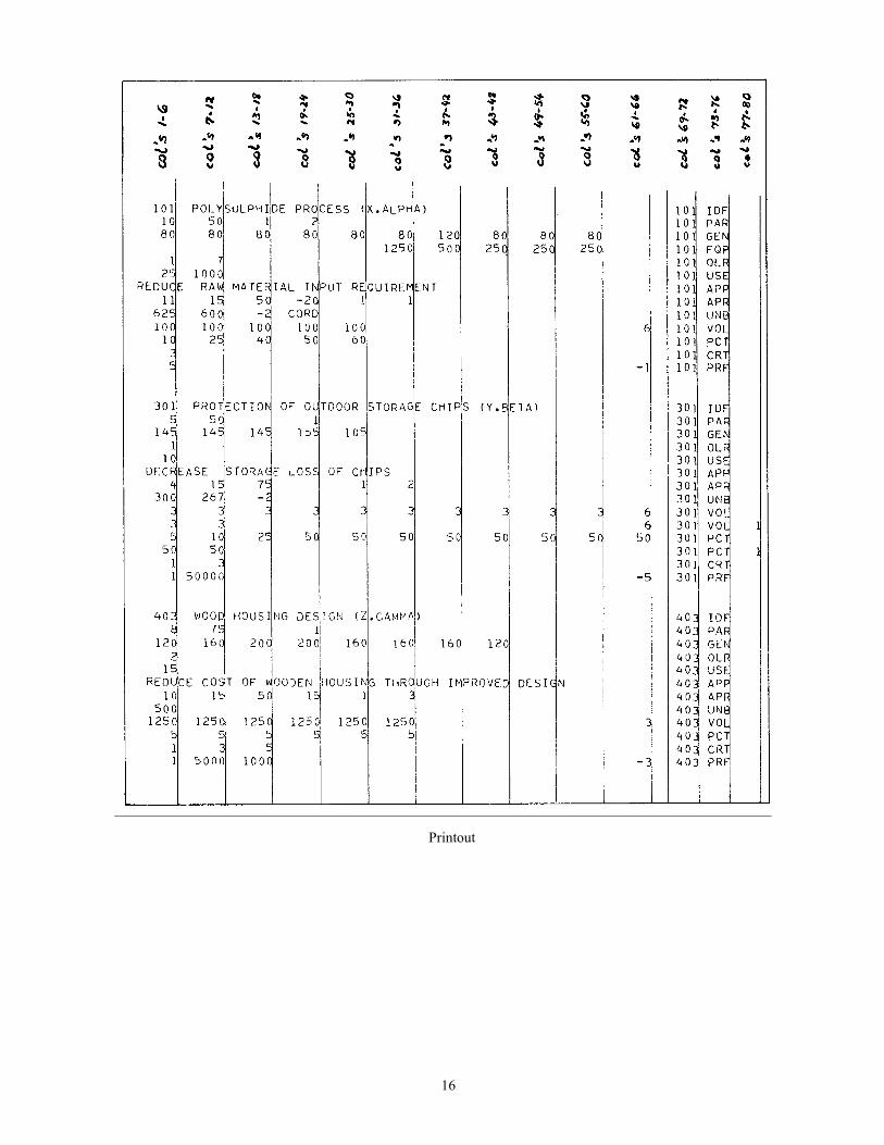
Printout

16

Card1 Coding2 Entries Card3

sequence pattern type

enter its value in front of the project code number, e.g., if the coefficient value for project 4 is "-3," the correct code is "-3004" DEP

M.1 S a. Number of projects whose coefficients are different from zero. MSC

b. Inequality code (See 1.1.b)

c. Co nstraint bound d. Scale factor–power of

10–to adjust entry c. e. Descriptive title: cols.

25-68 M.2 A Code numbers of projects

whose coefficients in the constraint specified are dif-ferent from zero MSC

M.3 A Coefficient values corres- VAL pondent to projects listed in M.2

1 See text: Data Formatting–Organization Data Cards.2 See A. General Instructions.3 Card type code word.

C—Operating Instructions

for Program ZERONE

Control Cards At most only two control cards are needed:

CC1 and CC2. The entries in card CC1 are: 1. Number of projects, i.e., rows of the basic

tableau: cols. 1-4. 2. Number of constraints, i.e., columns of the

basic tableau, except for column 0: cols. 5-8. 3. Number of sensitivity analysis options desired.

Blank if none: cols. 9-12. The entries in card CC2 are: Column 1: First sensitivity analysis option (A, B,

or C) wanted. Column 2: Second sensitivity analysis option (A,

B, or C) wanted, etc. Card CC2 is omitted if entry 3 in card CC1 is

blank.

Basic Tableau Cards The basic tableau cards input the basic informa-

tion matrix produced by program FILE (see chapter on Matrix Generation). For details on the card formats consult the eight FORTRAN V statements following the statement "10 CONTINUE" in the listing of program ZERONE. Note that MV : number of projects NC : number of constraints AZER0(1), I=1, MV : project benefits A(I,J), I=1, MV; J=1, NC : constraint coefficients JQ(J), J=1, NC : inequality indexed

"0" for ≥ "1" for ≤ "2" for =

B(J), J=1, NC : constraint bounds

Sensitivity Analysis Cards For each option Type A specified in control card

CC2, two sensitivity analysis cards are required: SA1 and SA2. The entries in card SA1 are:

1. Columns 4-6: blank if a constraint column of the basic tableau is modified (add, change or delete): "ACT" if a row of the basic tableau is modified.

2. Columns 7-12: number of constraint coeffi-cients modified.

3. Columns 13-18: new inequality sign when a constraint inequality is changed, blank otherwise.

4. Columns 19-24: new constraint bound in the modified row (column).

5. Columns 25-30: scale factor–power of 10–to adjust entry 4. Blank if not needed.

6. Columns 31-36: modification required, i.e., Blank if add one column (row)

"1" if delete one column (row) "2" if change one column (row).

7. Columns 37-42: column (row) number of array deleted or changed, blank otherwise.

8. Columns 45-80: explanatory title. Card SA2 is omitted if entry 6 in card SA1 is equal

to "1." The entries in card SA2 are the values of the non-zero coefficients of the modified column (row), together with their row (column) indexes. Eight-column fields are used to input such entries, the coefficient value in the first five columns and the coefficient index in the remaining three. Only 10 such composite entries can be fit into a card.

17

Consequently, more than one card is required if more than 10 are entered.

For each option Type B specified in control card CC2, one sensitivity analysis card (SB) is input. The entries in card SB are:

1. Columns 1-6: first constraint number in the sequence of constraints modified.

2. Columns 6-12: last constraint number in the sequence.

3. Columns 13-18: number of fixed increments desired in the constraint bounds.

4. Columns 19-24: additive or multiplicative incre-ment at each step.

5. Columns 25-30: scale factor–power of 10–to adjust entry 4.

6. Columns 31-36: blank if entry 4 specified an additive increment, "1" if entry, 4 specifies a multiplicative increment.

7. Columns 34-42: number of backward incre-ments required to adjust the magnitude of the constraint bounds after the last step is completed.

8. Columns 45-80: explanatory title.

No sensitivity analysis card is required for option Type C. As an example, suppose that card CC2 specified the option sequence CABCA. Then, the sensitivity analysis cards would be arranged in this sequence:

1. SA1 2. SA2 3. SB 4. SA1 5. SA2

And the ZERONE program would operate as follows: 1. Finds the optimum project mix on the basis of

the original basic tableau data. 2. Looks at the first project in the list and looks

up the original solution. If the project appears in the solution an exclusion constraint is imposed on the project, i.e., "the project must stay out." If the project does not appear in the solution an inclusion constraint is imposed on the project, namely, "the project must stay in." A new solution is found on the basis of the original data plus the additional constraint. The same process is repeated for each project in the list.

3. Modifies the original basic tableau according to the instructions contained in cards 1 and 2 and finds an optimum mix on the basis of the modified data.

4 Some constraint bounds are adjusted by a fixed increment according to the instructions in card 3. Entries 1 and 2 specify which constraints. Entries 4, 5, 6 specify the magnitude and type of the increment. The optimum project mix is found. These operations are repeated for as many steps as specified in entry 3. Before proceeding to the next sensitivity analysis the constraint bounds are readjusted as indicated in entry 7 of card 3.

5. Repeats operations specified under 2 above only this time starting from the basic tableau as modified through 3 and 4.

6. Modifies basic tableau according to instructions in cards 4 and 5 and then finds corresponding optimum solution.

18



A set of computer programs compiled for the information processing requirements of a model for evaluating research proposals are described. The programs serve to assemble and store information, periodically update it, and convert it to a form usable for decision-making. Guides for collecting and coding data are explained. The data-processing options available and instructions on operation of the software are outlined.

Oxford: 945.4: U65.012–U681.142. Retrieval Terms: research administration; proposal evaluation; analytical procedures; computer programs; mathematical models.













A data collection and processing procedure for evaluating a

Documents

Transcript of A data collection and processing procedure for evaluating a