A critical review of analytical methods for comprehensive ...
17
Water 2021, 13, 183. https://doi.org/10.3390/w13020183 www.mdpi.com/journal/water Supplementary Materials A critical review of analytical methods for comprehensive characterization of produced water Wenbin Jiang 1 , Lu Lin 1 , Xuesong Xu 1 , Xiaoxiao Cheng 1 , Yanyan Zhang 1 , Ryan Hall 2 , Pei Xu 1 * 1 Civil Engineering Department, New Mexico State University, Las Cruces, NM 88003, USA; [email protected] (W.J.); [email protected] (L.L.); [email protected] (X.X.); [email protected] (X.C.); [email protected] (Y.Z.) 2 NGL Water Solutions, NGL Energy Partners LP, Tulsa, Oklahoma 74136, USA; [email protected] * Correspondence: [email protected] 1. Produced Water Quality and Temporal Variability in Different Basins The United States produces large volumes of produced water (PW) from unconventional oil and gas development (UD). The production increase of the UD in the U.S. is mainly from seven key oil and gas basins: Appalachia including Marcellus and Utica (Pennsylvania, Ohio, and West Virginia), Bakken (North Dakota and Montana), Eagle Ford (South Texas), Haynesville (Louisiana and East Texas), Niobrara (Colorado and Wyoming), and the Permian Basin (West Texas and Southeast New Mexico) [1]. Table S1 summarizes the general physicochemical parameters of PW quality from primary UD plays in the U.S. Fig. S1 shows the temporal change of PW quality in Marcellus formation in Pennsylvania and Niobrara formation in Colorado. Because of the higher proportion of formation brine, PW typically has considerably higher total dissolved solids (TDS) concentrations than flowback water (FW). However, FW can have higher organics due to organic additives in fracturing fluid [2-4]. Fig. S1. Temporal variation of PW qualities in Marcellus shale, PA, two well sites [5]; and Niobrara formation, CO, two well sites [3,6]. 0 40000 80000 120000 160000 200000 0 5 10 15 20 25 30 Concentration (mg/L) Days Marcellus, PA TDS 1 TDS 2 Na 1 Na 2 Ca Cl 1 Cl 2 0 4000 8000 12000 16000 20000 24000 0 50 100 150 Concentration (mg/L) Days Niobrara, CO TDS 1 TDS 2 Na 1 Na 2 Ca Cl 1 Cl 2 TOC 1 TOC 2
Transcript of A critical review of analytical methods for comprehensive ...

Water 2021, 13, 183. https://doi.org/10.3390/w13020183 www.mdpi.com/journal/water
Supplementary Materials
A critical review of analytical methods for comprehensive characterization of produced water
Wenbin Jiang1, Lu Lin1, Xuesong Xu1, Xiaoxiao Cheng1, Yanyan Zhang1, Ryan Hall2, Pei Xu1*
1 Civil Engineering Department, New Mexico State University, Las Cruces, NM 88003, USA; [email protected]
(W.J.); [email protected] (L.L.); [email protected] (X.X.); [email protected] (X.C.); [email protected] (Y.Z.) 2 NGL Water Solutions, NGL Energy Partners LP, Tulsa, Oklahoma 74136, USA; [email protected]
* Correspondence: [email protected]
1. Produced Water Quality and Temporal Variability in Different Basins
The United States produces large volumes of produced water (PW) from unconventional oil and gas
development (UD). The production increase of the UD in the U.S. is mainly from seven key oil and gas
basins: Appalachia including Marcellus and Utica (Pennsylvania, Ohio, and West Virginia), Bakken
(North Dakota and Montana), Eagle Ford (South Texas), Haynesville (Louisiana and East Texas),
Niobrara (Colorado and Wyoming), and the Permian Basin (West Texas and Southeast New Mexico) [1].
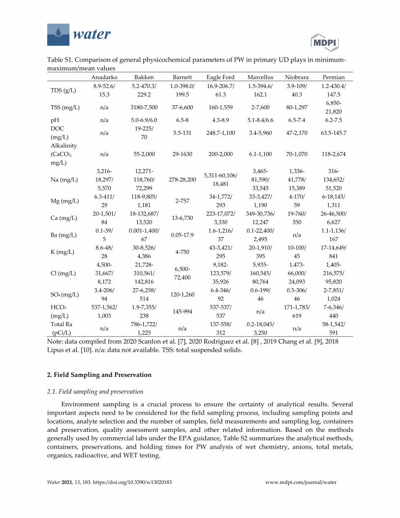
Table S1 summarizes the general physicochemical parameters of PW quality from primary UD plays in
the U.S. Fig. S1 shows the temporal change of PW quality in Marcellus formation in Pennsylvania and
Niobrara formation in Colorado. Because of the higher proportion of formation brine, PW typically has
considerably higher total dissolved solids (TDS) concentrations than flowback water (FW). However, FW
can have higher organics due to organic additives in fracturing fluid [2-4].
Fig. S1. Temporal variation of PW qualities in Marcellus shale, PA, two well sites [5]; and Niobrara
formation, CO, two well sites [3,6].
0
40000
80000
120000
160000
200000
0 5 10 15 20 25 30
Co
nce
ntr
atio
n (m
g/L
)
Days
Marcellus, PATDS 1
TDS 2
Na 1
Na 2
Ca
Cl 1
Cl 2
0
4000
8000
12000
16000
20000
24000
0 50 100 150
Co
nce
ntr
atio
n (m
g/L
)
Days
Niobrara, CO TDS 1
TDS 2
Na 1
Na 2
Ca
Cl 1
Cl 2
TOC 1
TOC 2
Water 2021, 13, 183. https://doi.org/10.3390/w13020183 www.mdpi.com/journal/water
Table S1. Comparison of general physicochemical parameters of PW in primary UD plays in minimum-
maximum/mean values Anadarko Bakken Barnett Eagle Ford Marcellus Niobrara Permian
TDS (g/L) 8.9-52.6/
15.3
5.2-470.3/
229.2
1.0-398.0/
199.5
16.9-206.7/
61.3
1.5-394.6/
162.1
3.9-109/
40.3
1.2-430.4/
147.5
TSS (mg/L) n/a 3180-7,500 37-6,600 160-1,559 2-7,600 80-1,297 6,850-
21,820
pH n/a 5.0-6.9/6.0 6.5-8 4.3-8.9 5.1-8.4/6.6 6.5-7.4 6.2-7.5
DOC
(mg/L) n/a
19-225/
70 5.5-131 248.7-1,100 3.4-5,960 47-2,170 63.5-145.7
Alkalinity
(CaCO3,
mg/L)
n/a 55-2,000 29-1630 200-2,000 6.1-1,100 70-1,070 118-2,674
Na (mg/L)
3,216-
18,297/
5,570
12,271-
118,760/
72,299
278-28,200 5,311-60,106/
18,481
3,465-
81,590/
33,545
1,336-
41,778/
15,389
316-
134,652/
51,520
Mg (mg/L) 6.3-411/
29
118-9,805/
1,181 2-757
34-1,772/
293
33-3,427/
1,190
4-170/
59
6-18,145/
1,311
Ca (mg/L) 20-1,501/
84
18-132,687/
13,520 13-6,730
223-17,072/
3,330
349-30,736/
12,247
19-760/
350
26-46,500/
6,627
Ba (mg/L) 0.1-39/
5
0.001-1,400/
67 0.05-17.9
1.6-1,216/
37
0.1-22,400/
2,495 n/a
1.1-1,136/
167
K (mg/L) 8.6-48/
28
30-8,526/
4,386 4-750
43-3,421/
295
20-1,910/
395
10-100/
45
17-14,649/
841
Cl (mg/L)
4,500-
31,667/
8,172
21,728-
310,561/
142,816
6,500-
72,400
9,182-
123,579/
35,926
5,935-
160,545/
80,764
1,473-
66,000/
24,093
1,405-
216,575/
95,820
SO4 (mg/L) 3.4-206/
94
27-6,258/
514 120-1,260
6.4-346/
92
0.6-199/
46
0.5-306/
46
2-7,851/
1,024
HCO3
(mg/L)
537-1,562/
1,003
1.9-7,355/
238 145-994
537-537/
537 n/a
171-1,783/
619
7-6,346/
440
Total Ra
(pCi/L) n/a
786-1,722/
1,225 n/a
137-558/
312
0.2-18,045/
3,250 n/a
58-1,542/
591
Note: data compiled from 2020 Scanlon et al. [7], 2020 Rodriguez et al. [8] , 2019 Chang et al. [9], 2018
Lipus et al. [10]. n/a: data not available. TSS: total suspended solids.
2. Field Sampling and Preservation
2.1. Field sampling and preservation
Environment sampling is a crucial process to ensure the certainty of analytical results. Several
important aspects need to be considered for the field sampling process, including sampling points and
locations, analyte selection and the number of samples, field measurements and sampling log, containers
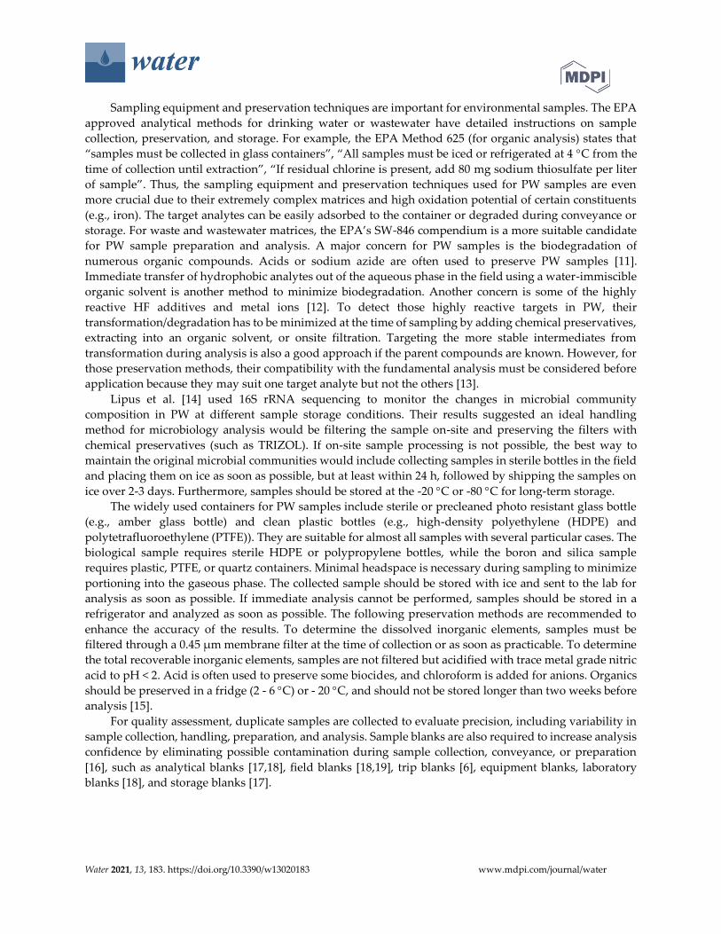
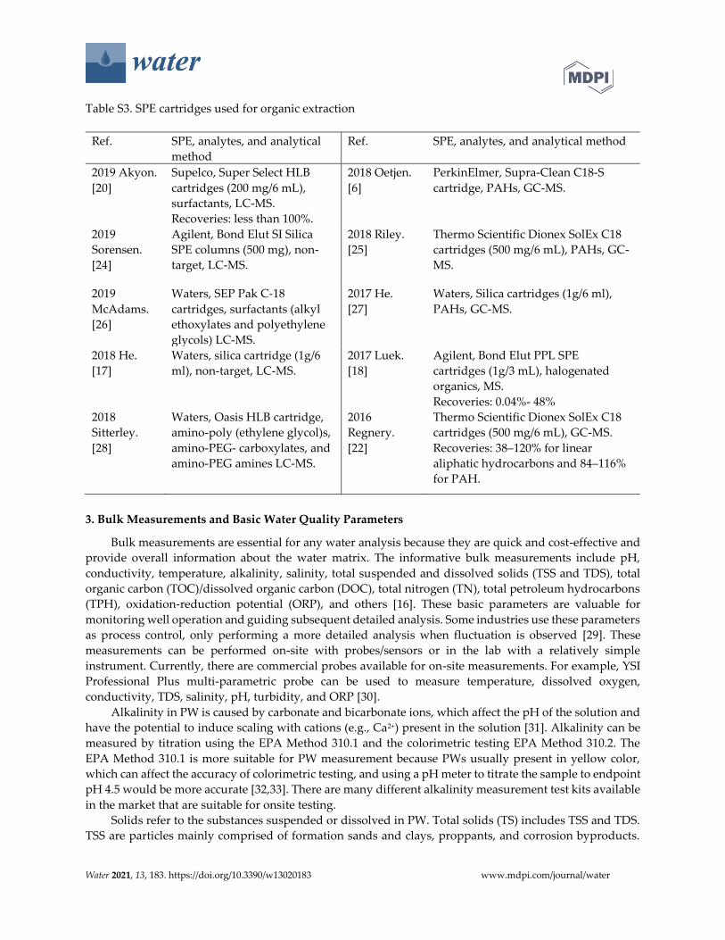
and preservation, quality assessment samples, and other related information. Based on the methods
generally used by commercial labs under the EPA guidance, Table S2 summarizes the analytical methods,
containers, preservations, and holding times for PW analysis of wet chemistry, anions, total metals,
organics, radioactive, and WET testing.
Water 2021, 13, 183. https://doi.org/10.3390/w13020183 www.mdpi.com/journal/water
Sampling equipment and preservation techniques are important for environmental samples. The EPA
approved analytical methods for drinking water or wastewater have detailed instructions on sample
collection, preservation, and storage. For example, the EPA Method 625 (for organic analysis) states that
“samples must be collected in glass containers”, “All samples must be iced or refrigerated at 4 C from the
time of collection until extraction”, “If residual chlorine is present, add 80 mg sodium thiosulfate per liter
of sample”. Thus, the sampling equipment and preservation techniques used for PW samples are even
more crucial due to their extremely complex matrices and high oxidation potential of certain constituents
(e.g., iron). The target analytes can be easily adsorbed to the container or degraded during conveyance or
storage. For waste and wastewater matrices, the EPA’s SW-846 compendium is a more suitable candidate
for PW sample preparation and analysis. A major concern for PW samples is the biodegradation of
numerous organic compounds. Acids or sodium azide are often used to preserve PW samples [11].
Immediate transfer of hydrophobic analytes out of the aqueous phase in the field using a water-immiscible
organic solvent is another method to minimize biodegradation. Another concern is some of the highly
reactive HF additives and metal ions [12]. To detect those highly reactive targets in PW, their
transformation/degradation has to be minimized at the time of sampling by adding chemical preservatives,
extracting into an organic solvent, or onsite filtration. Targeting the more stable intermediates from
transformation during analysis is also a good approach if the parent compounds are known. However, for
those preservation methods, their compatibility with the fundamental analysis must be considered before
application because they may suit one target analyte but not the others [13].
Lipus et al. [14] used 16S rRNA sequencing to monitor the changes in microbial community
composition in PW at different sample storage conditions. Their results suggested an ideal handling
method for microbiology analysis would be filtering the sample on-site and preserving the filters with
chemical preservatives (such as TRIZOL). If on-site sample processing is not possible, the best way to
maintain the original microbial communities would include collecting samples in sterile bottles in the field
and placing them on ice as soon as possible, but at least within 24 h, followed by shipping the samples on
ice over 2-3 days. Furthermore, samples should be stored at the -20 C or -80 C for long-term storage.
The widely used containers for PW samples include sterile or precleaned photo resistant glass bottle
(e.g., amber glass bottle) and clean plastic bottles (e.g., high-density polyethylene (HDPE) and
polytetrafluoroethylene (PTFE)). They are suitable for almost all samples with several particular cases. The
biological sample requires sterile HDPE or polypropylene bottles, while the boron and silica sample
requires plastic, PTFE, or quartz containers. Minimal headspace is necessary during sampling to minimize
portioning into the gaseous phase. The collected sample should be stored with ice and sent to the lab for
analysis as soon as possible. If immediate analysis cannot be performed, samples should be stored in a
refrigerator and analyzed as soon as possible. The following preservation methods are recommended to
enhance the accuracy of the results. To determine the dissolved inorganic elements, samples must be
filtered through a 0.45 µm membrane filter at the time of collection or as soon as practicable. To determine
the total recoverable inorganic elements, samples are not filtered but acidified with trace metal grade nitric
acid to pH < 2. Acid is often used to preserve some biocides, and chloroform is added for anions. Organics
should be preserved in a fridge (2 - 6 C) or - 20 C, and should not be stored longer than two weeks before
analysis [15].
For quality assessment, duplicate samples are collected to evaluate precision, including variability in
sample collection, handling, preparation, and analysis. Sample blanks are also required to increase analysis
confidence by eliminating possible contamination during sample collection, conveyance, or preparation
[16], such as analytical blanks [17,18], field blanks [18,19], trip blanks [6], equipment blanks, laboratory
blanks [18], and storage blanks [17].

Water 2021, 13, 183. https://doi.org/10.3390/w13020183 www.mdpi.com/journal/water
Table S2. Analyte containers, preservation, and holding times
Analyte Method (Technique) Sample
Container1
On-Site
Preservation
Holding
Time
Inorganic and Wet Chemistry
Alkalinity SM 2320 B-1997
(Titration) 250 mL - Plastic Cool to ≤ 6°C 14 Days1
Ammonia EPA 350.1
(Colorimetric) 250 mL - Plastic
H2SO4 until pH < 2,
Cool to ≤ 6°C 28 Days
Biochemical Oxygen
Demand (BOD5)
SM 5210 B-2001
(Titrimetric) 1000 mL - Plastic Cool to ≤ 6°C 48 Hours
Chemical Oxygen
Demand (COD)
EPA 410.4
(Spectrophotometric) 500 mL - Plastic
H2SO4 until pH < 2,
Cool to ≤ 6°C 28 Days
Chlorine, Total
Residual SM 4500 Cl- G 250 mL - Plastic Not required 15 Minutes
Dissolved Oxygen EPA 360.2 500 mL - Glass Not required 15 Minutes
Fluoride, Chloride,
Nitrite, Ortho-
Phosphate-p,
Bromide, Nitrate,
Sulfate Bromate,
Chlorite, Chlorate
EPA 300.0 (Ion
Chromatography) 500 mL - Plastic Cool to ≤ 6°C
28 Days
except NO2,
NO3, Ortho-
P 48 Hours
Fluoride, Chloride,
Nitrite, Ortho-
Phosphate, Bromide,
Nitrate, Sulfate
ASTM D4327
(Suppressed Ion
Chromatography)
500 mL - Plastic Cool to ≤ 6°C
28 Days
except NO2,
NO3, Ortho-
P 48 Hours
Hardness SM 2340B 250 mL - Plastic HNO3 until pH is <
2, Cool to ≤ 6°C 6 Months
Iodide EPA 345.1 250 mL - Plastic Cool to ≤ 6°C 24 Hours
Methylene Blue
Active Substances
(Surfactants, anionic)
EPA 425.1 250 mL - Plastic Cool to ≤ 6°C 48 Hours
N-Hexane
Extractable Material
(HEM) and Silica Gel
Treated N-Hexane
Extractable Material
(SGT-HEM)
EPA 1664A
(Gravimetric)
1 L - Wide-Mouth
Glass
HCl or H2SO4 until
pH < 2, Cool to ≤
6°C
28 Days
Water 2021, 13, 183. https://doi.org/10.3390/w13020183 www.mdpi.com/journal/water
Nitrogen, Ammonia SM 4500 NH3-B,C 500 mL - Plastic H2SO4 until pH < 2,
Cool to ≤ 6°C 28 Days
Nitrogen, Total
Kjeldahl
SM 4500Norg B,C
SM 4500 NH3-C 500 mL - Plastic
H2SO4 until pH < 2,
Cool to ≤ 6°C 28 Days
Phenolics EPA 420.4 1 L - Glass H2SO4 until pH < 2,
Cool to ≤ 6°C 28 Days
Phosphorous, Total ASTM D515 500 mL - Plastic H2SO4 until pH < 2,
Cool to ≤ 6°C 28 Days
Salinity SM 2520 250 mL - Plastic Cool to ≤ 6°C 28 Days
Silica EPA 200.7/6010 D 250 mL - Plastic Cool to ≤ 6°C 28 Days
Specific Conductance SM 2510 B-1997
(Conductivity Meter) 100 mL - Plastic Cool to ≤ 6°C 28 Days
Sulfate 300.0/375.4 500 mL - Plastic Cool to ≤ 6°C 28 Days
Sulfide SM 4500-S D 500 mL - Plastic
Cool to ≤ 6°C Zn
Acetate &
NaOH to pH > 9
7 Days
Sulfite SM 4500 SO3-B 100 mL - Plastic Not required 15 Minutes
Total Dissolved
Solids (TDS)
SM 2540 C-1997
(Gravimetric) 250 mL - Plastic Cool to ≤ 6°C 7 Days
Total Hardness SM 2340 C-1997
(Titrimetric) 250 mL - Plastic
HNO3 or H2SO4
until pH is < 2,
Cool to ≤ 6°C
6 Months
Total Organic Carbon
(TOC)
EPA 415.1 SM 5310
B-2000 (Combustion)
250 mL – Amber
Glass
H2SO4 or H3PO4
until pH < 2, Cool
to ≤ 6°C
28 Days
Total Suspended
Solids (TSS)
SM 2540 D-1997
(Gravimetric) 1000 mL - Plastic Cool to ≤ 6°C 7 Days
Turbidity EPA 180.1 100 mL - Plastic Cool to ≤ 6°C 28 Hours
Metals
Trace elements
(Total)
EPA 200.7 (ICP), EPA
200.8/EPA
6020B(ICPMS)
500 mL - Plastic HNO3 until pH is <
2 6 Months

Water 2021, 13, 183. https://doi.org/10.3390/w13020183 www.mdpi.com/journal/water
Trace elements
(Dissolved)
EPA 200.7 (ICP), EPA
200.8/EPA
6020B(ICPMS)
500 mL - Plastic
0.45 µm filtration in
15 minutes, HNO3
until pH is < 2
6 Months
Mercury
EPA 245.1 or 245.2
(Cold Vapor Atomic
Absorption)
500 mL - Plastic HNO3 until pH is <
2 28 Days
Hexavalent
Chromium
SM 3500 -Cr B-2009
(Colorimetric)/ EPA
7199
250 mL - Plastic Cool to ≤ 6°C 24 Hours
Organics
Alcohols EPA 8260C, 8270D,
and 8015C (GC/MS) 40-mL VOA vials
HCl until pH < 2,
Cool to ≤ 6°C 14 Days
Aldehydes EPA 8315(HPLC) 250 mL - Amber
Glass Cool to ≤ 6°C 3 Days
Diesel Range
EPA 3520C (sample
preparation) EPA
8015C (analysis) (GC)
1-L - Amber Glass Cool to ≤ 6°C 7 Days
Gasoline Range
EPA 5030B (sample
preparation) EPA
8015C (analysis) (GC)
40-mL VOA vials Cool to ≤ 6°C 7 Days
GCMS Purgeables EPA 524.2 40-mL VOA vials
Ascorbic acid and
HCl until pH < 2,
Cool to ≤ 6°C
14 Days
GCMS Purgeables EPA 624/8260C 40-mL VOA vials HCl until pH < 2,
Cool to ≤ 6°C 14 Days
Haloacetic Acids EPA 552.2 250 mL - Amber
Glass
Cool to ≤ 6°C,
NH4Cl 14 Days
Herbicides EPA 8151A (GC) 1-L - Amber Glass Cool to ≤ 6°C 7 Days
Oil & Grease
EPA 1664B
(Extraction and
Gravimetry)
1-L Amber Glass
HCl or H2SO4 until
pH < 2, Cool to ≤
6°C
28 Days
Pesticides EPA 608/8081B (GC) 1-L Amber Glass Cool to ≤ 6°C 7 Days
Semivolatile Organic
Compounds +
Tentative Identified
compounds
EPA 3520C/8270D
(GC /MS) 1-L - Amber Glass Cool to ≤ 6°C 7 Days

Water 2021, 13, 183. https://doi.org/10.3390/w13020183 www.mdpi.com/journal/water
Semivolatile Organic
Compounds +
Tentative Identified
compounds
EPA 625/8270D (GC) 1-L - Glass
Cool to ≤ 6°C, Add
Na2S2O3in the
presence of
residual chlorine
7 Days
Total Petroleum
Hydrocarbons
EPA 1664B
(Extraction and
Gravimetry)
1-L Amber Glass
HCl or H2SO4 until
pH < 2, Cool to ≤
6°C
28 Days
Volatile Organic
Compounds +
Tentative Identified
compounds
EPA 5030 or EPA
5035/8260C (GC/MS) 40-mL VOA vials
HCl until pH < 2,
Cool to ≤ 6°C 14 Days
Volatile Organic
Compounds +
Tentative Identified
compounds
EPA 624.1 (GC /MS) 40-mL VOA vials
HCl until pH < 2,
Cool to ≤ 6°C, Add
Na2S2O3 (a few
crystals) in the
presence of
residual chlorine
14 Days
Radioactive
Total Radium 226
(Liquid Samples)
EPA 903.1 (Radon
Emanation) 1-L - Plastic
HNO3 until pH is <
2 6 Months
Total Radium 228
(Liquid Samples)
EPA 904.0
(Radiochemical/Preci
pitation)
1-L - Plastic HNO3 until pH is <
2 6 Months
Total Radium 226
and 228 (Solid
Samples)
EPA 901.1 (Gamma
Spectroscopy)
215 grams - Wide-
Mouth Plastic None 6 Months
Gross Alpha/Beta
(Liquid Samples)
EPA 900.0
(Evaporation)
500 mL – Wide-
Mouth Plastic
HNO3 until pH is <
2 6 Months
Gross Alpha/Beta
(Solid Samples)
EPA 900.0
(Evaporation)
30 grams - Wide-
Mouth Plastic None 6 Months
Microbiological
Coliform, Fecal SM 9222D 250 mL - Sterile
Plastic Cool to ≤ 6°C 8 Hours
Coliform, Fecal Strep SM 9230A/B 250 mL - Sterile
Plastic Cool to ≤ 6°C 6 Hours
Coliform, Total EPA 1603 250 mL - Sterile
Plastic Cool to ≤ 6°C 8 Hours
Coliform, E.Coli EPA 1603 250 mL - Sterile
Plastic Cool to ≤ 6°C 8 Hours
Enterococci EPA 1600 250 mL - Sterile
Plastic Cool to ≤ 6°C 8 Hours

Water 2021, 13, 183. https://doi.org/10.3390/w13020183 www.mdpi.com/journal/water
Heterotrophic Plate
Count SM 9215B
250 mL - Sterile
Plastic Cool to ≤ 6°C 8 Hours
Whole Effluent Toxicity (WET)
Acute Nonvertebrate Ceriodaphnia dubia
EPA 2002.0
4-L - Plastic
Cubitainer Cool to ≤ 6°C 36 Hours
Acute Vertebrate Pimephales promelas
EPA 2000.0
4-L - Plastic
Cubitainer Cool to ≤ 6°C 36 Hours
Chronic
Nonvertebrate
Ceriodaphnia dubia
EPA 1002.0
4-L - Plastic
Cubitainer Cool to ≤ 6°C 36 Hours
Chronic Vertebrate Pimephales promelas
EPA 1000.0
4-L - Plastic
Cubitainer Cool to ≤ 6°C 36 Hours
1. Alkalinity: 14 days holding time for treated samples and should be analyzed as soon as possible for
untreated samples.
2.2. Sample preparation
Sample preparation is essential for PW analysis. It has several goals: 1) to concentrate or dilute target
analytes to meet the capability of analytical instrumentation; 2) to remove materials in the matrix that might
interfere with the chromatographic separation, ionization, or detection of target analytes. For inorganic
analysis, these goals are usually met by removing particles and diluting the sample to meet instrument
performance. For organic compound analyses, removing inorganic ions in PW while retaining specific
organics in the final solution is often required. The EPA’s SW-846 compendium consists of over 200
analytical methods for sampling and analyzing waste and other matrices. It includes the 3000 series for
inorganic sample preparation, 3500 series for organic sample extraction, and 3600 series for organic extract
cleanup. A variety of sample preparation methods suitable for PW samples are discussed in the following
sections.
2.2.1 Dilution, filtration, and centrifugation
Dilution is a useful way to address the sample matrix, making it more suitable for the analytical
instrument and adjusting the concentration of analytes into the calibration range. Filtration and
centrifugation are two simple sample preparation methods. They both remove particulate materials in PW
to make samples compatible with analytical methods and protect instruments, such as to prevent clogging
and high backpressure for ion chromatography (IC) and liquid chromatography (LC) columns [20].
However, filtration and centrifugation do not concentrate the sample or change the dissolved fraction of
the sample matrix, which may be required when analyzing PW, especially when targeting trace amounts
of organic analytes. Thus, these methods usually can only be applied to bulk and inorganic measurements
and need to be coupled with other pretreatment methods for organic sample analysis [21]. Another
important consideration for these methods is their bias toward chemical constituents adsorbed to the
suspended solids in the matrix, which are often removed during the filtration process [13]. Thus, the filtered
solids are sometimes collected and treated (e.g., acid digested) to analyze the PW sample comprehensively
[17].
2.2.2 Solid-phase extraction
Solid-phase extraction (SPE) is a powerful and widely used extraction technique that offers high
selectivity, flexibility, and automation. The EPA Method 3535A is a procedure for isolating target organic
analytes from aqueous samples using SPE media. SPE has been widely applied to concentrate and purify
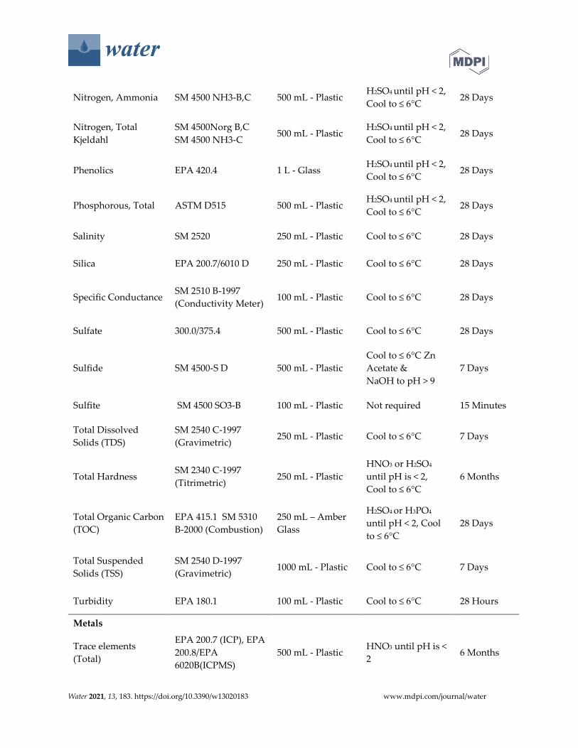
analytes from different water matrices, including wastewater and PW [6,22,23]. Table S3 summarizes the
SPE cartridges used in literature for organic analysis.
Water 2021, 13, 183. https://doi.org/10.3390/w13020183 www.mdpi.com/journal/water
Table S3. SPE cartridges used for organic extraction
Ref. SPE, analytes, and analytical
method
Ref. SPE, analytes, and analytical method
2019 Akyon.
[20]
Supelco, Super Select HLB
cartridges (200 mg/6 mL),
surfactants, LC-MS.
Recoveries: less than 100%.
2018 Oetjen.
[6]
PerkinElmer, Supra-Clean C18-S
cartridge, PAHs, GC-MS.
2019
Sorensen.
[24]
Agilent, Bond Elut SI Silica
SPE columns (500 mg), non-
target, LC-MS.
2018 Riley.
[25]
Thermo Scientific Dionex SolEx C18
cartridges (500 mg/6 mL), PAHs, GC-
MS.
2019
McAdams.
[26]
Waters, SEP Pak C-18
cartridges, surfactants (alkyl
ethoxylates and polyethylene
glycols) LC-MS.
2017 He.
[27]
Waters, Silica cartridges (1g/6 ml),
PAHs, GC-MS.
2018 He.
[17]
Waters, silica cartridge (1g/6
ml), non-target, LC-MS.
2017 Luek.
[18]
Agilent, Bond Elut PPL SPE
cartridges (1g/3 mL), halogenated
organics, MS.
Recoveries: 0.04%- 48%
2018
Sitterley.
[28]
Waters, Oasis HLB cartridge,
amino-poly (ethylene glycol)s,
amino-PEG- carboxylates, and
amino-PEG amines LC-MS.
2016
Regnery.
[22]
Thermo Scientific Dionex SolEx C18
cartridges (500 mg/6 mL), GC-MS.
Recoveries: 38–120% for linear
aliphatic hydrocarbons and 84–116%
for PAH.
3. Bulk Measurements and Basic Water Quality Parameters
Bulk measurements are essential for any water analysis because they are quick and cost-effective and
provide overall information about the water matrix. The informative bulk measurements include pH,
conductivity, temperature, alkalinity, salinity, total suspended and dissolved solids (TSS and TDS), total
organic carbon (TOC)/dissolved organic carbon (DOC), total nitrogen (TN), total petroleum hydrocarbons
(TPH), oxidation-reduction potential (ORP), and others [16]. These basic parameters are valuable for
monitoring well operation and guiding subsequent detailed analysis. Some industries use these parameters
as process control, only performing a more detailed analysis when fluctuation is observed [29]. These
measurements can be performed on-site with probes/sensors or in the lab with a relatively simple
instrument. Currently, there are commercial probes available for on-site measurements. For example, YSI
Professional Plus multi-parametric probe can be used to measure temperature, dissolved oxygen,
conductivity, TDS, salinity, pH, turbidity, and ORP [30].
Alkalinity in PW is caused by carbonate and bicarbonate ions, which affect the pH of the solution and
have the potential to induce scaling with cations (e.g., Ca2+) present in the solution [31]. Alkalinity can be
measured by titration using the EPA Method 310.1 and the colorimetric testing EPA Method 310.2. The
EPA Method 310.1 is more suitable for PW measurement because PWs usually present in yellow color,
which can affect the accuracy of colorimetric testing, and using a pH meter to titrate the sample to endpoint
pH 4.5 would be more accurate [32,33]. There are many different alkalinity measurement test kits available
in the market that are suitable for onsite testing.
Solids refer to the substances suspended or dissolved in PW. Total solids (TS) includes TSS and TDS.
TSS are particles mainly comprised of formation sands and clays, proppants, and corrosion byproducts.

Water 2021, 13, 183. https://doi.org/10.3390/w13020183 www.mdpi.com/journal/water
TDS are primarily charged particles (major cations and anions). TDS levels can vary considerably in a given
region. For example, PW in Bakken shale varies from 1,800 to 350,000 mg/L TDS [9]. There are two principal
methods for measuring TDS: gravimetric analysis and conductivity. The gravimetric method is more
accurate than the conductivity method, while the latter is more convenient. Dilution is often required for
the conductivity method to yield accurate results within the instrument measurement range. Currently, TS,
TSS, and TDS are often measured by the Standard Methods 2540 A-F (gravimetric methods, range up to
20,000 mg/L) approved by the EPA to analyze solids residue from domestic and industrial wastewater [34].
TS is measured by evaporating a well-mixed sample in a weighed dish and dried to constant weight in an
oven at 103 to 105 ºC. The increase in dish weight represents the TS (method 2540B). TSS and TDS can be
measured at the same time. A well-mixed sample is first filtered through a weighed standard glass-fiber
filter. The residue retained on the filter is dried to a constant weight at 103 to 105 ºC; the filter weight
increase represents the TSS (method 2540D). TDS is obtained by evaporating the filtrate in a weighed dish
and dried to constant weight at 180 ºC; the dish weight increase represents the TDS (method 2540C) [32,35].
TOC provides the concentration of organic carbon in water. It is a more convenient and accurate
measurement to perform in the lab than biochemical oxygen demand (BOD) or chemical oxygen demand
(COD) methods. The EPA Method 415.3 or the Standard Method 5310C is usually used to measure TOC.
Samples are first acidified by HCl, H3PO4, or H2SO4 to pH < 2, to remove the inorganic carbon (carbonate
and bicarbonate). The organic carbon is then oxidized to carbon dioxide by combustion or chemical
oxidation, which is then detected by a conductivity detector or a nondispersive infrared (NDIR) detector
[36]. DOC is another commonly measured parameter representing the dissolved (filtered) organic
compounds in water. The procedure requires the sample to be filtered by a 0.45 m filter before analysis
by a TOC analyzer (e.g., Shimadzu TOC analyzer TOC-L or TOC-V series) [37]. Dilution sometimes is
needed when the concentration of DOC exceeds the optimum range of the instrument [38].
TN is the sum of the inorganic nitrogen, organic nitrogen, and ammonia. Inorganic nitrite and nitrate
are analyzed using the EPA Method 353.2: nitrate in a filtered sample is reduced to nitrite, then all the
nitrite is measured colorimetrically. The sum of organic nitrogen and ammonia can be analyzed using EPA
Methods 351.2 and EPA-NERL 351.4. The sample is digested to convert total Kjeldahl nitrogen (total
nitrogen in organic substances and inorganic ammonia/ammonium) into ammonia. Then the concentration
of ammonia is measured using an ion-selective electrode [32,33]. Another method (ASTM D8083) to
determine TN is to convert all nitrogen compounds to NO, followed by photoelectric measurement of
radiation emitted when NO2 relaxes [39].
These methods are easy to perform if the samples are correctly prepared. Dilution is usually a
convenient way to avoid interferences because these bulk parameters do not measure constituents at trace
levels. Table S1 includes some measurement results of the typical water quality parameters from different
PW sources.
4. Organic Analysis
Table S4 summarizes 25 peer-reviewed publications analyzing organic compounds in shale gas PW
from 2016 to date. In summary, 14 publications used LC-MS, while 13 used GC-based techniques (the
overlap is because some publications used both techniques). This trend may be a result of advances in
HRMS and ultra-HRMS, in addition to the concerns surrounding undisclosed proprietary chemicals used
during HF and their transformation products during well production. Orbitrap (7 publications) and Q-ToF
(7 publications) have become the dominant HRMS/MS analyzers because of their high resolution and
relatively low price. In comparison, only 2 publications from the same group used FT-ICR-MS, likely due
to its high cost despite the high resolution.

Water 2021, 13, 183. https://doi.org/10.3390/w13020183 www.mdpi.com/journal/water
Table S4. Summary of the recent studies analyzing organic compounds in PW
Ref. Basin/formation,
sample Target analytes Pretreatment methods Analytical methods Quantified
2020 Almaraz.
[38]
DJ basin (CO),
PW
Iodinated organic
compounds (5 volatile IOCs)
during biological treatment
of FPW
IOCs are treated by
polydimethylsiloxane/divinyl
benzene (PDMS/DVB) fiber
HS-SPME-GC-MS(QQQ);
Iodide double-junction ion-
selective electrode
YES
2019 Akyon.
[20]
Utica and Bakken
shales, PW
Total, dissolved organic
carbon during biological
treatment
LLE (DCM) for GC-MS;
SPE for LC-MS. Super Select
HLB cartridges (200 mg/6 mL,
Supelco)
GC-MS (Q) for SVOCs;
LC-MS (Q-ToF) for
surfactants
YES
2019 Sorensen.
[24]
Norwegian
North Sea oil
field, PW
Total organic extracts
(TOEs);
Nontarget analysis
LLE (DCM) for TOEs;
Silica SPE cartridge (Agilent
Bond Elut SI)
Some samples derivatized
with BSFTA.
GC-FID for GC-amenable
compounds;
GC-MS (Q) for decalins,
PAHs, alkylated PAHs and
C0-9 phenols;
GC X GC-MS (ToF) and LC-
HRMS (Orbitrap) for non-
target analysis
YES
2019 Sun.
[40]
Duvernay
Formation
(Canada), FPW
over 30 days of
flowback
Nontarget profiling.
Identified 7 series of
homologues composed of
ethylene oxide and 2 series
of alkyl ethoxylates
LLE (DCM)
HPLC-HRMS (Orbitrap), ESI
both positive and negative
mode
Semi-
quantified
2019 Wang.
[41]
Bakken shale
(ND), FW;
Barnett shale
(TX), FW; DJ
basin (CO), PW
DOM n/a
3D EEM fluorescence
spectroscopy and FRI
analysis
YES

Water 2021, 13, 183. https://doi.org/10.3390/w13020183 www.mdpi.com/journal/water
2019
McAdams.
[26]
Marcellus Shale
(PA), FW
Alkyl ethoxylates (AEOs)
and polyethylene glycols
(PEGs)
SPE, SEP Pak C-18 cartridges
(Waters) LC-HRMS (Q-ToF) NO
2018
Butkovskyi.
[21]
Baltic shale
(Poland), PW
(after 2 months)
DOC and individual organic
compounds removal during
treatment
All samples filtered by 0.45
m filter;
MS sample filtered by 0.2 m
filter;
Dilution.
Volatile fatty acids (VFA)
and alcohols: GC-FID;
Headspace gas: GC-TCD;
Organic compounds: LC-
HRMS (Linear Ion Trap
Orbitrap)
Semi-
quantified
2018 He.
[17]
Duvernay
Formation
(Canada), FW
Non-target analysis and
targeted PAH analysis
0.4 m filters to separated
solid and aqueous; LLE
(DCM and hexane) to extract
organics from liquid; SPE to
clean samples, silica cartridge
(Waters)
HPLC-HRMS (Orbitrap) NO
2018
Hildenbrand.
[30]
Eagle Ford (TX),
PW
Comprehensive analysis of
PW during treatment No pretreatment
HSGC: VOCs;
GC-MS: SVOCs.
Semi-
quantified
2018 Luek.
[19]
Marcellus shale
(WV), fracturing
fluid (FF), FW,
and PW
Temporal change of
halogenated organic
compounds (iodinated are
dominant)
Through a 0.7 mm glass fiber
filter (Whatman GF/F);
SPE: 1 g/6 mL Bond Elut PPL
cartridges
Bruker Solarix 12T
electrospray ionization FT-
ICR-MS
Semi-
quantified
2018 Oetjen.
[6]
Niobrara
formation (DJ
basin, CO). FW
Temporal change of organic
compounds throughout the
flowback period
Hydrophobic: SPE
(automated, AutoTrace 280
SPE unit), Supra-Clean C18-S
cartridge (PerkinElmer);
Hydrophilic: salt assisted LLE
(NaCl with acetonitrile).
Hydrophilic: HPLC- MS (Q-
ToF)
Hydrophobic: GC-MS (Q)
Semi-
quantified

Water 2021, 13, 183. https://doi.org/10.3390/w13020183 www.mdpi.com/journal/water
2018 Oetjen.
[42]
CO, HF
wastewater spill
simulation
5 PEGs, 8 BACs, 14 AEOs.
Filtered with 0.45 m PES
filters;
Salt assisted LLE (NaCl with
acetonitrile)
LC-MS (Q-ToF) NO
2018 Nell.
[43]
Marcellus shale
(WV), PW, and
FW
19 HF additives, the matrix
effects on the ionization
efficiency
Filtered with 0.45 m PTFE
filters;
Dilution
LC-MS (Q-Orbitrap) YES
2018 Lyman.
[44]
Uinta basin (UT),
Upper green
river basin (WY).
PW
Methane, non-methane
hydrocarbons (C2-C11), light
alcohols, and carbon dioxide
Purge and trap
GC-FID for light
hydrocarbons (ethane,
ethylene, acetylene, propane,
and propylene).
GC-MS for the rest
compounds.
YES
2018 Riley.
[25]
Piceance basin
(CO) PW;
Denver-Julesburg
(DJ) basin (CO)
PW, and DJ basin
(CO) FW
Dissolved organic matter
(DOC) during treatment
LC-HRMS: Salt assisted LLE
(NaCl with Acetonitrile)
GC-MS: automated SPE
(AutoTrace 280, Thermo
Scientific). Octadecyl-bonded
silica cartridges
LC-MS (Q-ToF): low
molecular weight organics.
GC-MS (single Q): semi-
volatile aliphatic and
aromatic hydrocarbons.
3D fluorescence.
YES
2018 Sitterley.
[28]
CO, OK, TX, WY,
ND. FW and PW
Amino-poly (ethylene
glycol)s, amino-
poly(ethylene glycol)
carboxylates, and amino-
poly(ethylene glycol) amines
SPE, Oasis HLB cartridge
(Waters Corporation) HPLC-HRMS (Q-ToF) NO
2018 Tasker.
[45]
Marcellus shale
(PA), FW
Organics from O&G
wastewater used on a road LLE (DCM)
GC X GC - MS (ToF): diesel
and gas range organics. NO
2018 Varona-
Torres.
[46]
Permian Basin,
west TX. Soil
BETX in soil, close to UD
activities
Room temperature ionic
liquids (RTILs) as solvents for
HSGC
HS-GC-MS (QQQ) YES
Water 2021, 13, 183. https://doi.org/10.3390/w13020183 www.mdpi.com/journal/water
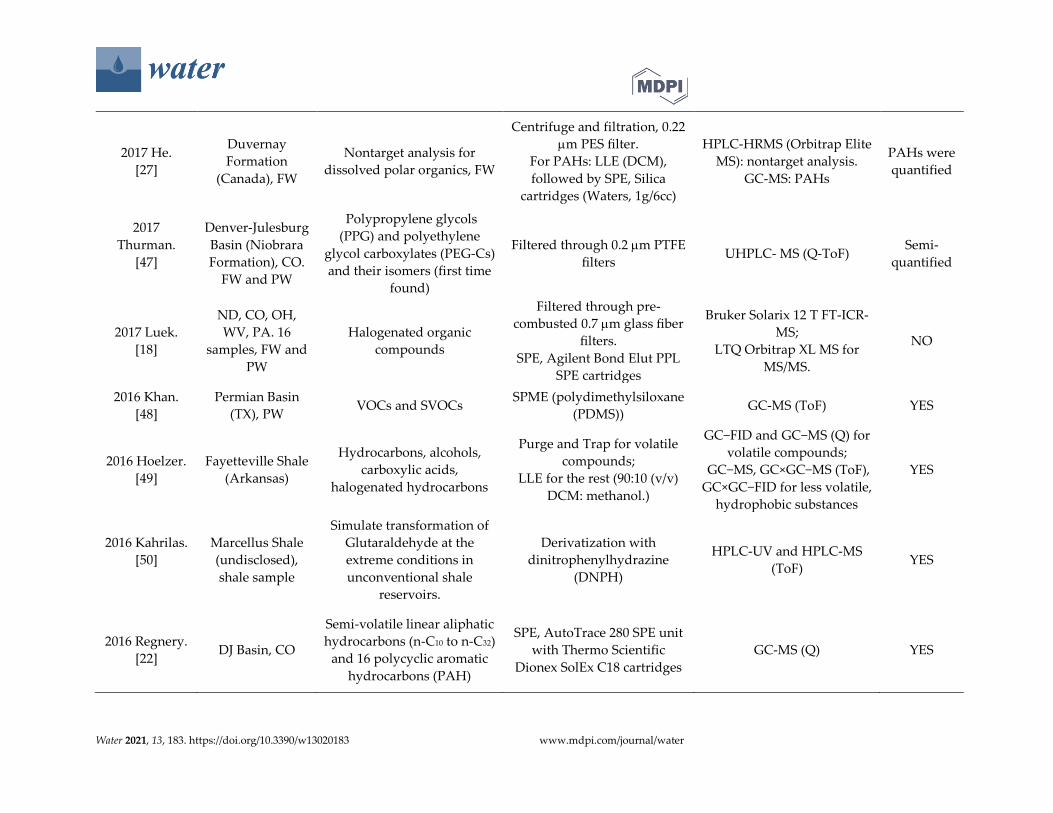
2017 He.
[27]
Duvernay
Formation
(Canada), FW
Nontarget analysis for
dissolved polar organics, FW
Centrifuge and filtration, 0.22
m PES filter.
For PAHs: LLE (DCM),
followed by SPE, Silica
cartridges (Waters, 1g/6cc)
HPLC-HRMS (Orbitrap Elite
MS): nontarget analysis.
GC-MS: PAHs
PAHs were
quantified
2017
Thurman.
[47]
Denver-Julesburg
Basin (Niobrara
Formation), CO.
FW and PW
Polypropylene glycols
(PPG) and polyethylene
glycol carboxylates (PEG-Cs)
and their isomers (first time
found)
Filtered through 0.2 m PTFE
filters UHPLC- MS (Q-ToF)
Semi-
quantified
2017 Luek.
[18]
ND, CO, OH,
WV, PA. 16
samples, FW and
PW
Halogenated organic
compounds
Filtered through pre-
combusted 0.7 m glass fiber
filters.
SPE, Agilent Bond Elut PPL
SPE cartridges
Bruker Solarix 12 T FT-ICR-
MS;
LTQ Orbitrap XL MS for
MS/MS.
NO
2016 Khan.
[48]
Permian Basin
(TX), PW VOCs and SVOCs
SPME (polydimethylsiloxane
(PDMS)) GC-MS (ToF) YES
2016 Hoelzer.
[49]
Fayetteville Shale
(Arkansas)
Hydrocarbons, alcohols,
carboxylic acids,
halogenated hydrocarbons
Purge and Trap for volatile
compounds;
LLE for the rest (90:10 (v/v)
DCM: methanol.)
GC−FID and GC−MS (Q) for
volatile compounds;
GC−MS, GC×GC−MS (ToF),
GC×GC−FID for less volatile,
hydrophobic substances
YES
2016 Kahrilas.
[50]
Marcellus Shale
(undisclosed),
shale sample
Simulate transformation of
Glutaraldehyde at the
extreme conditions in
unconventional shale
reservoirs.
Derivatization with
dinitrophenylhydrazine
(DNPH)
HPLC-UV and HPLC-MS
(ToF) YES
2016 Regnery.
[22] DJ Basin, CO
Semi-volatile linear aliphatic
hydrocarbons (n-C10 to n-C32)
and 16 polycyclic aromatic
hydrocarbons (PAH)
SPE, AutoTrace 280 SPE unit
with Thermo Scientific
Dionex SolEx C18 cartridges
GC-MS (Q) YES

Water 2021, 13, 183. https://doi.org/10.3390/w13020183 www.mdpi.com/journal/water
References:
1. U.S.EIA. Drilling Productivity Report. 2020.
2. Fisher, C.; Jack, R. Analysis of ions in hydraulic fracturing wastewaters using ion chromatography. In
Hydraulic Fracturing: Environmental Issues, ACS Publications: 2015; pp. 135-150.
3. Kim, S.; Omur-Ozbek, P.; Dhanasekar, A.; Prior, A.; Carlson, K. Temporal analysis of flowback and
produced water composition from shale oil and gas operations: impact of frac fluid characteristics.
Journal of Petroleum Science and Engineering 2016, 147, 202-210.
4. Rosenblum, J.; Nelson, A.W.; Ruyle, B.; Schultz, M.K.; Ryan, J.N.; Linden, K.G. Temporal
characterization of flowback and produced water quality from a hydraulically fractured oil and gas
well. Science of The Total Environment 2017, 596, 369-377.
5. Barbot, E.; Vidic, N.S.; Gregory, K.B.; Vidic, R.D. Spatial and temporal correlation of water quality
parameters of produced waters from Devonian-age shale following hydraulic fracturing.
Environmental science & technology 2013, 47, 2562-2569.
6. Oetjen, K.; Chan, K.E.; Gulmark, K.; Christensen, J.H.; Blotevogel, J.; Borch, T.; Spear, J.R.; Cath, T.Y.;
Higgins, C.P. Temporal characterization and statistical analysis of flowback and produced waters and
their potential for reuse. Science of the Total Environment 2018, 619, 654-664.
7. Scanlon, B.R.; Reedy, R.C.; Xu, P.; Engle, M.; Nicot, J.; Yoxtheimer, D.; Yang, Q.; Ikonnikova, S. Can
we beneficially reuse produced water from oil and gas extraction in the US? Science of The Total
Environment 2020, 717, 137085.
8. Rodriguez, A.Z.; Wang, H.; Hu, L.; Zhang, Y.; Xu, P. Treatment of Produced Water in the Permian
Basin for Hydraulic Fracturing: Comparison of Different Coagulation Processes and Innovative Filter
Media. Water 2020, 12, 770.
9. Chang, H.; Li, T.; Liu, B.; Vidic, R.D.; Elimelech, M.; Crittenden, J.C. Potential and implemented
membrane-based technologies for the treatment and reuse of flowback and produced water from
shale gas and oil plays: A review. Desalination 2019, 455, 34-57.
10. Lipus, D.; Roy, D.; Khan, E.; Ross, D.; Vikram, A.; Gulliver, D.; Hammack, R.; Bibby, K. Microbial
communities in Bakken region produced water. FEMS microbiology letters 2018, 365, fny107.
11. Vanderford, B.J.; Mawhinney, D.B.; Trenholm, R.A.; Zeigler-Holady, J.C.; Snyder, S.A. Assessment of
sample preservation techniques for pharmaceuticals, personal care products, and steroids in surface
and drinking water. Analytical and bioanalytical chemistry 2011, 399, 2227-2234.
12. Kahrilas, G.A.; Blotevogel, J.; Stewart, P.S.; Borch, T. Biocides in hydraulic fracturing fluids: a critical
review of their usage, mobility, degradation, and toxicity. Environmental science & technology 2014, 49,
16-32.
13. Oetjen, K.; Giddings, C.G.; McLaughlin, M.; Nell, M.; Blotevogel, J.; Helbling, D.E.; Mueller, D.;
Higgins, C.P. Emerging analytical methods for the characterization and quantification of organic
contaminants in flowback and produced water. Trends in Environmental Analytical Chemistry 2017, 15,
12-23.
14. Lipus, D.; Vikram, A.; Hammack, R.; Bibby, K.; Gulliver, D. The Effects of Sample Storage Conditions
on the Microbial Community Composition in Hydraulic Fracturing Produced Water. Geomicrobiology
Journal 2019, 36, 630-638.
15. Santos, I.C.; Hildenbrand, Z.L.; Schug, K.A. A Review of Analytical Methods for Characterizing the
Potential Environmental Impacts of Unconventional Oil and Gas Development. Analytical chemistry
2018, 91, 689-703.
16. Carlton Jr, D.D.; Hildenbrand, Z.L.; Schug, K.A. Analytical Approaches for High-Resolution
Environmental Investigations of Unconventional Oil and Gas Exploration. In Advances in Chemical
Pollution, Environmental Management and Protection, Elsevier: 2017; Vol. 1, pp. 193-226.

Water 2021, 13, 183. https://doi.org/10.3390/w13020183 www.mdpi.com/journal/water
17. He, Y.; Sun, C.; Zhang, Y.; Folkerts, E.J.; Martin, J.W.; Goss, G.G. Developmental toxicity of the
organic fraction from hydraulic fracturing flowback and produced waters to early life stages of
Zebrafish (Danio rerio). Environmental science & technology 2018, 52, 3820-3830.
18. Luek, J.L.; Schmitt-Kopplin, P.; Mouser, P.J.; Petty, W.T.; Richardson, S.D.; Gonsior, M. Halogenated
organic compounds identified in hydraulic fracturing wastewaters using ultrahigh resolution mass
spectrometry. Environmental science & technology 2017, 51, 5377-5385.
19. Luek, J.L.; Harir, M.; Schmitt-Kopplin, P.; Mouser, P.J.; Gonsior, M. Temporal dynamics of
halogenated organic compounds in Marcellus Shale flowback. Water research 2018, 136, 200-206.
20. Akyon, B.; McLaughlin, M.; Hernández, F.; Blotevogel, J.; Bibby, K. Characterization and biological
removal of organic compounds from hydraulic fracturing produced water. Environmental Science:
Processes & Impacts 2019, 21, 279-290.
21. Butkovskyi, A.; Faber, A.-H.; Wang, Y.; Grolle, K.; Hofman-Caris, R.; Bruning, H.; Van Wezel, A.P.;
Rijnaarts, H.H. Removal of organic compounds from shale gas flowback water. Water research 2018,
138, 47-55.
22. Regnery, J.; Coday, B.D.; Riley, S.M.; Cath, T.Y. Solid-phase extraction followed by gas
chromatography-mass spectrometry for the quantitative analysis of semi-volatile hydrocarbons in
hydraulic fracturing wastewaters. Analytical methods 2016, 8, 2058-2068.
23. Cluff, M.A.; Hartsock, A.; MacRae, J.D.; Carter, K.; Mouser, P.J. Temporal changes in microbial
ecology and geochemistry in produced water from hydraulically fractured Marcellus Shale gas wells.
Environmental science & technology 2014, 48, 6508-6517.
24. Sørensen, L.; McCormack, P.; Altin, D.; Robson, W.J.; Booth, A.M.; Faksness, L.-G.; Rowland, S.J.;
Størseth, T.R. Establishing a link between composition and toxicity of offshore produced waters using
comprehensive analysis techniques–A way forward for discharge monitoring? Science of The Total
Environment 2019, 694, 133682.
25. Riley, S.M.; Ahoor, D.C.; Regnery, J.; Cath, T.Y. Tracking oil and gas wastewater-derived organic
matter in a hybrid biofilter membrane treatment system: A multi-analytical approach. Science of the
Total Environment 2018, 613, 208-217.
26. McAdams, B.C.; Carter, K.E.; Blotevogel, J.; Borch, T.; Hakala, J.A. In situ transformation of hydraulic
fracturing surfactants from well injection to produced water. Environmental Science: Processes &
Impacts 2019, 21, 1777-1786.
27. He, Y.; Flynn, S.L.; Folkerts, E.J.; Zhang, Y.; Ruan, D.; Alessi, D.S.; Martin, J.W.; Goss, G.G. Chemical
and toxicological characterizations of hydraulic fracturing flowback and produced water. Water
research 2017, 114, 78-87.
28. Sitterley, K.A.; Linden, K.G.; Ferrer, I.; Thurman, E.M. Identification of proprietary amino ethoxylates
in hydraulic fracturing wastewater using liquid chromatography/time-of-flight mass spectrometry
with solid-phase extraction. Analytical chemistry 2018, 90, 10927-10934.
29. Hickenbottom, K.L.; Hancock, N.T.; Hutchings, N.R.; Appleton, E.W.; Beaudry, E.G.; Xu, P.; Cath,
T.Y. Forward osmosis treatment of drilling mud and fracturing wastewater from oil and gas
operations. Desalination 2013, 312, 60-66.
30. Hildenbrand, Z.L.; Santos, I.C.; Liden, T.; Carlton Jr, D.D.; Varona-Torres, E.; Martin, M.S.; Reyes,
M.L.; Mulla, S.R.; Schug, K.A. Characterizing variable biogeochemical changes during the treatment
of produced oilfield waste. Science of the Total Environment 2018, 634, 1519-1529.
31. Wasylishen, R.; Fulton, S. Reuse of flowback and produced water for hydraulic fracturing in tight oil.
Pet. Technol. Alliance Can 2012.
32. U.S.EPA. Clean Water Act Analytical Methods. 2019.
33. U.S.EPA. EPA 600/4‐79‐020 Methods for Chemical Analysis of Water and Wastes. 1983.
34. Mass (1990) Crop salt tolerance. In: Agricutlral Assessment and Mangament Manual.

Water 2021, 13, 183. https://doi.org/10.3390/w13020183 www.mdpi.com/journal/water
35. Rice, E.W.; Baird, R.B.; Eaton, A.D.; Clesceri, L.S. Standard methods for the examination of water and
wastewater. American Public Health Association, Washington, DC 2012, 541.
36. EPA, U. Method 415.3: Determination of Total Organic Carbon and Specific UV Absorbance at 254
Nm in Source Water and Drinking Water. Revision: 2009.
37. Potter, B.; Wimsatt, J. Method 415.3. Measurement of total organic carbon, dissolved organic carbon
and specific UV absorbance at 254 nm in source water and drinking water. US Environmental
Protection Agency, Washington, DC 2005.
38. Almaraz, N.; Regnery, J.; Vanzin, G.F.; Riley, S.M.; Ahoor, D.C.; Cath, T.Y. Emergence and fate of
volatile iodinated organic compounds during biological treatment of oil and gas produced water.
Science of The Total Environment 2020, 699, 134202.
39. International, A. Standard Test Method for Total Nitrogen, and Total Kjeldahl Nitrogen (TKN) by
Calculation, in Water by High Temperature Catalytic Combustion and Chemiluminescence
Detection. 2016.
40. Sun, C.; Zhang, Y.; Alessi, D.S.; Martin, J.W. Nontarget profiling of organic compounds in a temporal
series of hydraulic fracturing flowback and produced waters. Environment international 2019, 131,
104944.
41. Wang, H.; Lu, L.; Chen, X.; Bian, Y.; Ren, Z.J. Geochemical and microbial characterizations of
flowback and produced water in three shale oil and gas plays in the central and western United
States. Water research 2019, 164, 114942.
42. Oetjen, K.; Blotevogel, J.; Borch, T.; Ranville, J.F.; Higgins, C.P. Simulation of a hydraulic fracturing
wastewater surface spill on agricultural soil. Science of the Total Environment 2018, 645, 229-234.
43. Nell, M.; Helbling, D.E. Exploring matrix effects and quantifying organic additives in hydraulic
fracturing associated fluids using liquid chromatography electrospray ionization mass spectrometry.
Environmental Science: Processes & Impacts 2019, 21, 195-205.
44. Lyman, S.N.; Mansfield, M.L.; Tran, H.N.; Evans, J.D.; Jones, C.; O'Neil, T.; Bowers, R.; Smith, A.;
Keslar, C. Emissions of organic compounds from produced water ponds I: Characteristics and
speciation. Science of the Total Environment 2018, 619, 896-905.
45. Tasker, T.; Burgos, W.D.; Piotrowski, P.; Castillo-Meza, L.; Blewett, T.; Ganow, K.; Stallworth, A.;
Delompré, P.; Goss, G.; Fowler, L.B. Environmental and human health impacts of spreading oil and
gas wastewater on roads. Environmental science & technology 2018, 52, 7081-7091.
46. Varona-Torres, E.; Carlton Jr, D.D.; Hildenbrand, Z.L.; Schug, K.A. Matrix-effect-free determination
of BTEX in variable soil compositions using room temperature ionic liquid co-solvents in static
headspace gas chromatography mass spectrometry. Analytica chimica acta 2018, 1021, 41-50.
47. Thurman, E.M.; Ferrer, I.; Rosenblum, J.; Linden, K.; Ryan, J.N. Identification of polypropylene
glycols and polyethylene glycol carboxylates in flowback and produced water from hydraulic
fracturing. Journal of hazardous materials 2017, 323, 11-17.
48. Khan, N.A.; Engle, M.; Dungan, B.; Holguin, F.O.; Xu, P.; Carroll, K.C. Volatile-organic molecular
characterization of shale-oil produced water from the Permian Basin. Chemosphere 2016, 148, 126-136.
49. Hoelzer, K.; Sumner, A.J.; Karatum, O.; Nelson, R.K.; Drollette, B.D.; O’Connor, M.P.; D’Ambro, E.L.;
Getzinger, G.J.; Ferguson, P.L.; Reddy, C.M. Indications of transformation products from hydraulic
fracturing additives in shale-gas wastewater. Environmental science & technology 2016, 50, 8036-8048.
50. Kahrilas, G.A.; Blotevogel, J.; Corrin, E.R.; Borch, T. Downhole transformation of the hydraulic
fracturing fluid biocide glutaraldehyde: implications for flowback and produced water quality.
Environmental science & technology 2016, 50, 11414-11423.