A Critical Quantity for Noise Attenuation in Feedback …qnie/Publications/ja52.pdfA Critical...

A Critical Quantity for Noise Attenuation in FeedbackSystemsLiming Wang, Jack Xin, Qing Nie*

Center for Mathematical and Computational Biology, Center for Complex Biological Systems, and Department of Mathematics, University of California at Irvine, Irvine,

California, United States of America

Abstract

Feedback modules, which appear ubiquitously in biological regulations, are often subject to disturbances from the input,leading to fluctuations in the output. Thus, the question becomes how a feedback system can produce a faithful responsewith a noisy input. We employed multiple time scale analysis, Fluctuation Dissipation Theorem, linear stability, andnumerical simulations to investigate a module with one positive feedback loop driven by an external stimulus, and weobtained a critical quantity in noise attenuation, termed as ‘‘signed activation time’’. We then studied the signed activationtime for a system of two positive feedback loops, a system of one positive feedback loop and one negative feedback loop,and six other existing biological models consisting of multiple components along with positive and negative feedbackloops. An inverse relationship is found between the noise amplification rate and the signed activation time, defined as thedifference between the deactivation and activation time scales of the noise-free system, normalized by the frequency ofnoises presented in the input. Thus, the combination of fast activation and slow deactivation provides the best noiseattenuation, and it can be attained in a single positive feedback loop system. An additional positive feedback loop oftenleads to a marked decrease in activation time, decrease or slight increase of deactivation time and allows larger kinetic ratevariations for slow deactivation and fast activation. On the other hand, a negative feedback loop may increase the activationand deactivation times. The negative relationship between the noise amplification rate and the signed activation time alsoholds for the six other biological models with multiple components and feedback loops. This principle may be applicable toother feedback systems.

Citation: Wang L, Xin J, Nie Q (2010) A Critical Quantity for Noise Attenuation in Feedback Systems. PLoS Comput Biol 6(4): e1000764. doi:10.1371/journal.pcbi.1000764

Editor: Christopher V. Rao, University of Illinois at Urbana-Champaign, United States of America

Received May 6, 2009; Accepted March 25, 2010; Published April 29, 2010

Copyright: � 2010 Wang et al. This is an open-access article distributed under the terms of the Creative Commons Attribution License, which permitsunrestricted use, distribution, and reproduction in any medium, provided the original author and source are credited.

Funding: This work was supported by NIH grants R01GM75309, R01GM67247, and P50GM76516. The funders had no role in study design, data collection andanalysis, decision to publish, or preparation of the manuscript.

Competing Interests: The authors have declared that no competing interests exist.

* E-mail: [email protected]

Introduction

It has been identified that feedback loops play important roles in

a variety of biological processes, such as calcium signaling [1,2],

p53 regulation [3], galactose regulation [4], cell cycle [5–8], and

budding yeast polarization [9–13]. Although the detailed regula-

tion of feedback loops may vary in different systems, the overall

functions of feedback loop modules may be similar. For example,

positive feedback loops are mainly used for promoting bi-stable

switches and amplifying signals. One example is the cell cycle

system [5–8] in which the mitotic regulator CDK1 activates

Cdc25, which in turn activates CDK1, forming a positive feedback

loop. Conversely, Wee1 and CDK1 inactivate each other, forming

a double-negative feedback loop, equivalent to a positive feedback

loop. The overall positive feedback regulation gives rise to a bi-

stable switch that toggles between the inter-phase state and the

mitotic-phase state. Another example is the system of yeast mating

[9–15], in which multi-stage positive feedback loops enable the

localization of signaling molecules at the plasma membrane by

amplifying signals to initiate cell polarization and mating.

While most studies of feedback loops have been concerned with

their roles in signal amplification, switch (or switch-like) responses

[16–20], and oscillations [21] (See [22,23] for the latest review.),

recently, another important aspect of feedback loops has drawn

more and more attention: modulating (accelerating or delaying)

timing of signal responses [22,24,25]. Intuitively, positive feedback

could amplify signals inducing an expeditious activation, or delay

an activation by setting a higher threshold such that the system is

activated only when the response accumulates beyond that

threshold [22,25]. Because characteristics of noises (e.g., the

temporal frequency of a noise) in a biological process are closely

related to timing of a signaling system, feedbacks clearly play a

critical role in noise attenuation [26–29].

Thus, one of the central questions on noise analysis is how the

architecture of a feedback circuit affects its noise property. Some

studies suggested that positive feedbacks tended to amplify noise

and negative feedbacks typically attenuated noise [30–32]; on the

other hand, some other studies demonstrated that the positive

feedbacks could attenuate noises and there were no strong

correlations between the sign of feedbacks (negative or positive)

and the noise attenuation properties [28,33].

In their novel work [34], Brandman et al. linked the effect of

positive feedback loops on noise attenuation to the time scales of

the feedback loops. They studied a canonical feedback module

consisting of three components, i.e., an output C and two positive

feedback loops, A and B. The output C is turned on by the two

positive feedback loops and B, which are stimulated by an external

(or upstream) stimulus and are also facilitated by C (Figure 1A).

PLoS Computational Biology | www.ploscompbiol.org 1 April 2010 | Volume 6 | Issue 4 | e1000764

The output C becomes active (or stays inactive) as the pulse

stimulus is high (or low). Through numerical simulations, Brand-

man et al. [34] showed that, if one of the positive feedback loops

(e.g., loop A) was slow and the other one was fast (termed as dual-

time loops), the system could lead to distinct active output C even

in the presence of noise in the stimulus (at the high state).

Following this work, Zhang et al. [35] studied dual-time loops in

producing a bi-stable response with a constant input (unlike a pulse

input in [34]). They concluded that dual-time loops were the most

robust design among all combinations in producing bi-stable

output for a slightly different system in which the stimulus could

activate A or B without the participation of C. Kim et al. [36]

considered systems coupled with negative and positive feedback

loops. By assuming all the positive feedback loops have the same

time scale but different time delays, they obtained a system that

was capable of performing fast activation, fast deactivation, and

noise attenuation.

What remains unclear are the sufficient and necessary

conditions for a feedback system to achieve noise attenuation.

Are two, or at least two, positive feedback loops (as used in [34–

36]) required for controlling noise amplification in the input? Is a

fast loop necessary for a positive feedback loop system to achieve

noise attenuation? Are there any intrinsic quantities that connect

the dynamic property of a system in absence of noises with the

system’s capability of noise suppression? If such quantities exist,

how do positive feedbacks or negative feedbacks affect them?

In this work, we find that the capability of noise suppression in a

system strongly depends on a quantity that measures the difference

between the deactivation and activation times relative to the input

noise frequency. Specifically, this quantity, termed as the ‘‘signed

activation time’’, has an inverse relationship with the noise

amplification rate, with larger signed activation time leading to

better noise attenuation. In addition, the signed activation time ,

representing one of the essential temporal characteristics of the

system in absence of noises, may be controlled by either negative

or positive feedbacks. We explore the properties of the quantity

through both analytic approach (including linear stability analysis,

multiple time scale analysis, and Fluctuation Dissipation Theorem)

and numerical simulations. We first consider the same modules as

in [34], and find that, for example, an additional positive feedback

loop could drastically increase the signed activation time by

speeding up the activation time while still keeping the deactivation

time slow, as consistent with the previous observation [34] that

dual-time-loop systems suppress noises better than single-loop

systems. We next add a negative feedback loop to the positive-

feedback-only system and show that a negative feedback loop

usually slows down both activation and deactivation processes,

leading to better or worse noise attenuation depending on which

process (between activation and deactivation) is more significantly

affected. Finally, we study the signed activation time and its

relations to the noise amplification rate in different systems

involving various feedbacks (e.g., positive, negative, and feedfor-

ward), including a yeast cell polarization model [14,37], a

polymyxin B resistance model in enteric bacteria [38], and four

connector-mediated models [39]. All simulations confirm that the

capability of noise attenuation in those systems improves as the

signed activation time increases.

Results

The Difference between Deactivation and ActivationTime Scales Dictates Noise Attenuation Ability

A simple model with one positive feedback loop may have two

components with one upstream stimulus (inside the red dashed

Figure 1. Schematic diagrams of single-positive-loop, positive-positive-loop, and positive-negative-loop modules. (A) Thepositive feedback modules. In this plot, there are three components:loop A, loop B, and output C. A, B, and C denote the active forms,whereas A’, B’, and C’ stand for the corresponding inactive forms,respectively. The red dashed box represents the single-positive-loopmodule consisting of B and C only. In the B component, signals comein to active B with the help of C at the rate of kctb . All other activationprocesses of B are lumped into one term, the basal activation rate k4tb .The conversion from B to B’ has the rate tb . In the C component, C isactivated by B at the rate of k1 , and the deactivation of C is at the rateof k2 . The basal activation rate of C is k3 . Similar notations are used inthe A component. (B) The positive-negative-loop module. The positivefeedback from A to C is replaced by negative feedback (red arrow).doi:10.1371/journal.pcbi.1000764.g001

Author Summary

Many biological systems use feedback loops to regulatedynamic interactions among different genes and proteins.Here, we ask how interlinked feedback loops control thetiming of signal transductions and responses and, conse-quently, attenuate noise. Drawing on simple modelingalong with both analytical insights and computationalassessments, we have identified a key quantity, termed asthe ‘‘signed activation time’’, that dictates a system’s abilityof attenuating noise. This quantity combining the speed ofdeactivation and activation in signal responses, relative tothe input noise frequency, is determined by the propertyof feedback systems when noises are absent. In general,such quantity could be measured experimentally throughthe output response time of a signaling system driven bypulse stimulus. This principle for noise attenuation infeedback loops may also be applicable to other biologicalsystems involving more complex regulations.

Minimal Design Constraints for Noise Attenuation


box in Figure 1A). In this system, the output C is activated by B,

and B is triggered by a stimulus s and regulated by C. The

stimulus s drives the output of the system with a high (or low)

stimulus that corresponds to an active (or inactive) state of C.

Many biological circuits have positive feedback regulations of this

nature [1,2,19,40]. For example, C is a kinase to phosphorylate B’to B, and once B is activated, it catalyzes a conversion from an

inactive form C’ to an active form C [5]. Neglecting the

mechanistic details, while keeping the essential interactions, we

model the dynamics of the above module by the following system

of ordinary differential equations (Text S1):

dc

dt~k1b 1{cð Þ{k2czk3

db

dt~ kcsc 1{bð Þ{bzk4ð Þtb,

ð1Þ

where c and b represent normalized concentrations of C and B,

respectively. The normalized stimulus s, as a function of time, t,usually varies (continuously) between two states, i.e., an inactive

state in which s~0 (or the ‘‘off’’ state) and an active state in which

s~1 (or the ‘‘on’’ state). The parameters kc, k1, k2, and k3 are

kinetic constants, and tb indicates the time scale for loop B.

Once the output of the system reaches the ‘‘on’’ state driven by

the stimulus, how does system (1) respond to temporal noises in the

input signal s? What are the strategies for effectively maintaining

the system in the ‘‘on’’ state even with noises presented by the

stimulus? We find that the time scales, denoted by t1?0 and t0?1

(Figure 2), for the system to switch from the ‘‘on’’ state to the ‘‘off’’

state and from ‘‘off’’ to ‘‘on’’ respectively in the absence of noises

in the signal, play a critical role. Specifically, when t1?0{t0?1ð Þ is

significantly larger than the time scale of the noise, i.e.,

t1?0{t0?1ð Þ&1=v, where v is the frequency of the noise, the

output C of the system remains in the ‘‘on’’ state (Figures 3A–3B).

Intuitively, when the system in the stable ‘‘on’’ state receives a

noisy signal with an instantaneous value possibly near s~0, it

needs time t1?0 to react and detour to the ‘‘off’’ state. In the case

of t1?0&1=v, before the system settles down to the ‘‘off’’ state, a

noisy signal with an instantaneous value near s~1 shows up,

forcing the system to synchronize with the new value of the input

signal. If t0?1%1=v, the output recovers fast from the drift

towards the inactive state, and is more likely to maintain around

the ‘‘on’’ state. The above intuition suggests that the noise

attenuation at the ‘‘on’’ state depends positively on t1?0v and

negatively on t0?1v. Thus, the quantity t1?0{t0?1ð Þv, i.e., the

signed activation time , could be a good indicator of a system’s

ability of attenuating noise.

To investigate how noise level in the solution depends on the

signed activation time , we study the noise amplification rate,

defined as the relative ratio of the coefficients of variation of the

output (gc) and the noise (gs) [28]:

r2 : ~gc

gs

~std cð Þ=ScTstd sð Þ=SsT

:

First, we perform numerical simulations on system (1) (Methods) to

study the relationship between r2 and t1?0{t0?1ð Þv by varying

the activation and deactivation time scales while fixing v. This is

achieved by changing the kinetic parameteres k1,k2,kc, and tb

individually in the system, and r2 is found decreasing in

t1?0{t0?1ð Þv (Figure 3C). Next, we hold t1?0{t0?1ð Þ constant,

corresponding to no changes in all parameters, and vary the noise

frequency v. The trend of r2 remains the same (Figure 3D). We

also consider the dependence of r2 on t1?0 and t0?1 individually

(Figure S1). In the single loop case, it turns out that r2 is always

decreasing in t1?0 (Figures S1A–S1C), but it might be increasing

in t0?1 (Figure S1D). Similar results are also obtained for positive-

positive-loop systems (Figure S2). Both suggest that neither

deactivation nor activation alone can fully characterize the noise

amplification rate, and the noise amplification rate is more likely

determined by the difference between the deactivation and

activation time scales. Next, we further explore this system

through the following two analytical approaches.

Two-time-scale analysis. To understand why the relative

ratio of the time scale of noise in the input and the system’s

intrinsic time scales when noise is absent is important to noise

Figure 2. Schematic illustration of the activation (left) and deactivation (right) time scales.doi:10.1371/journal.pcbi.1000764.g002



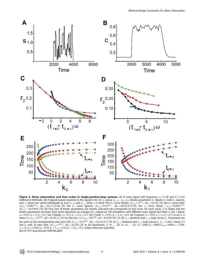
Figure 3. Noise attenuation and time scales in single-positive-loop systems. (A) A noisy signal with frequency v~1=40 and Es~0:62(defined in Methods). (B) A typical output response to the signal in (A). (C) r2 versus t1?0{t0?1ð Þv. Kinetic parameters k1 (black), k2 (red), kc (green),and tb (blue) are varied individually to tune t1?0 and t0?1 while v is fixed. The k1 curve (black): k1ð Þn~eDk1n, Dk1~ln 10ð Þ=20; the k2 curve (red):k2ð Þn~0:06eDk2n , Dk2~ln 1:2=0:06ð Þ=20; the kc curve (green): kcð Þn~0:5eDkcn , Dkc~ln(10=0:5)=20; the tb curve (blue): tbð Þn~0:005eDtbn,Dtb~{ln 0:005ð Þ=20. (D) Four sets of kinetic parameters are chosen, and each set corresponds to one curve. On each curve, v is varied, and thekinetic parameters are fixed. Each point represents an average of r2 based on 100 simulations with different noisy signals but fixed v. Set 1 (blue):tb~0:01, k1~3, k2~0:3. Set 2 (black): tb~0:1, k1~3, k2~0:3. Set 3 (red): tb~0:01, k1~3, k2~0:6. Set 4 (green): tb~0:01, k1~1, k2~0:3. In set 2, vtakes 1=vð Þm~2eDdm, Dd~ln 50=2ð Þ=10. For the rest, 1=vð Þm~20eDdm , Dd~ln 100=20ð Þ=10. (E) t0?1 (bottom) and t1?0 (top) versus kc . Parameters are

the same as the corresponding color set in (D). kcð Þn~0:5eDkcn , Dkc~ln 10=0:5ð Þ=20. (F) t0?1 (bottom) and t1?0 (top) versus k1 . kc~1 (set 1, blue), 0:5(set 2, red). In each plot, k1ð Þn~eDk1n , Dk1~ln 10ð Þ=20. In all simulations, n~0, . . . ,20, m~0, . . . ,10, T1~2000,T2~4000,Tmax~6000,t1~2300,t2~T2,k3~0:001,k4~0:01,kc~1,tb~0:01,k1~3,k2~0:3, unless otherwise specified.doi:10.1371/journal.pcbi.1000764.g003



attenuation, we carry out a two-time-scale asymptotic expansion of

the solutions [41]. The solutions are first written in terms of two

time scales, tz~t and ~tt~et, where e~tb,

c tz,~ttð Þ~c0 tz,~ttð Þzec1 tz,~ttð Þze2c2 tz,~ttð Þz � � � ,

b tz,~ttð Þ~b0 tz,~ttð Þzeb1 tz,~ttð Þze2b2 tz,~ttð Þz � � � :ð2Þ

When e is small, the two time scales are well separated. The

independent variables tz and ~tt correspond to the fast and

slow time scales, respectively. This two-time-scale asymptotic

expansion allows us to see a clear dependence of solutions on

different time scales. For fast varying input, the input s tz,~ttð Þ can

be written as the sum of a constant signal s0 and a fast altering

term s1 tzð Þ, i.e., s tz,~ttð Þ~s0zs1 tzð Þ. The solution of (1) is (Text

S1, Section 4)

c tz,~ttð Þ~ c0{k1b0 ~ttð Þzk3

k1b0 ~ttð Þzk2

� �e{ k1b0

~ttð Þzk2ð Þtzzk1b0 ~ttð Þzk3

k1b0 ~ttð Þzk2

zO eð Þ,

b tz,~ttð Þ~b0 ~ttð ÞzO eð Þ:

ð3Þ

Here, b0 and c0 are the initial conditions of b and c, respectively;

b0 is the solution of

db0

d~tt~kcs0 1{b0ð Þ k1b0zk3

k1b0zk2{b0zk4: ð4Þ

The zero-order solution, c0,b0ð Þ, approximates the full solution

when e is small (Figures S3A–S3C), and we thus focus on the noise

effect on the zero-order solution. Notice that the noise term s1 tzð Þdoes not show up in equation (4), so the zero-order approximations

with and without noise are the same, suggesting that fast varying

noises are filtered out through the system (Figures S3D–S3E).

If the input consists of both fast and slow noises (Figures S3G–

S3H), for example, when the input is decoupled to a sum of fast

and slow noise terms, i.e., s tz,~ttð Þ~s0zs1 tzð Þzs2 ~ttð Þ, then only

the slow part appears in the equation of b0 (Text S1, Section 4),

db0

d~tt~kcs2 ~ttð Þ 1{b0ð Þ k1b0zk3

k1b0zk2{b0zk4:

In this case, the noise term s2 ~ttð Þ could significantly affect the

output (Figures S3F, S3I–S3J). In summary, the single-positive-

loop system could function as a low-pass filter [42–45], and thus

the time scale of the input noise relative to the time scales of the

internal system is important to noise attenuation.

Fluctuation Dissipation Theorem (FDT) approach. To

see the inverse relation between the noise amplification rate

and the signed activation time , we employ the FDT approach

[27,28,46,47]. Under the linear approximation assumption in

FDT, the noise amplification rate can be computed analytically

(Text S1, Section 5), and when tb%1 and tb=v%1, we obtain

r22&

tb=v

SsT Kakc{1ð Þ Kaz1ð Þ kc

kcz1

, ð5Þ

where Ka : ~k1=k2 is the association constant, indicating the

strength of the activation from B to C.

Based on equation (5), one can infer a qualitative relation

between the noise amplification rate and the kinetic parame-

ters. For Ka, since Kakcw1 (Text S1, Section 1, the conditions

for a ‘‘switch-like’’ response), as Ka increases, the noise am-

plification rate r2 decreases. The parameter kc, measuring the

activation from C to B, negatively affects the noise amplifica-

tion rate, and the time scale of the B-loop, tb, positively

affects r2.

On the contrary, t1?0{t0?1ð Þ depends negatively on tb and

positively on Ka and kc (details later). Thus, a negative relation

between t1?0{t0?1ð Þ and r2 is expected (as confirmed by

simulations in Figures 3C–3D). In addition, tb and v appearing

together in (5) suggests a close dependence of the noise attenuation

capability on the noise frequency in the input and the intrinsic

time scales of the system in the absence of noise.

How to Control Deactivation and Activation Time ScalesIn the previous section, we have demonstrated that the noise

amplification rate depends negatively on the signed activation time.

Thus, if a system is persistent to noise at the ‘‘on’’ state, it should have

a large signed activation time . In this section, by studying the

dynamics of the noise-free system, we show that a small tb is

necessary for a slow deactivation, but not sufficient. With a fixed small

tb, larger kc or Ka could lead to slower deactivation and faster

activation.

Deactivation. When the input signal switches from s~1 to

s~0, the system responds through deactivation from the stabilized

active state to the inactive state. The dynamics of c around the

inactive state can be approximated by (Text S1, Section 1)

c tð Þ& c�0{b�0k1 k2{k3ð Þk1k4zk2ð Þ2

!e{ k1k4zk2ð Þt

zb�0k1 k2{k3ð Þk1k4zk2ð Þ2

e{tbtz�cc0:

ð6Þ

Here, �cc0 and �bb0 denote the steady state values of c and b at s~0,

respectively; c�0,b�0� �

~ c0{�cc0,b0{�bb0

� �, where c0 and b0 are the

initial conditions of c and b, respectively. Equation (6) clearly

indicates that the dynamics of c is not only determined by

parameters in the c-equation but also affected by the time scale

of the b-equation, tb. Without the positive feedback loop (b-

equation), c can be solved in a closed form:

c tð Þ~ c0{k3

k2

� �e{k2tz

k3

k2: ð7Þ

Comparing (7) with (6), it is clear that, to achieve a slower

deactivation when b is present, tb need to be much smaller than

k2. Conversely, if tb is on the same or higher order of k2, the

output c responds in a time scale of 1=k2 without slow

deactivation.

In addition to a small tb, the more significantly the second term

in (6) contributes to the dynamics of c, the slower c tð Þ converges to

�cc0, and thus, the larger t1?0 becomes. The contribution of e{tbt to

the deactivation time scale is characterized by (Text S1, Section 1)

Kaz1ð Þ kc

kcz1: ð8Þ

As a result, a large Ka or kc leads to a slow deactivation.

This is also demonstrated by direct simulations (Figures 3E–3F, top).

In addition to the linear stability analysis around either the

active state or the inactive state, under the assumption of tb%k2,



our previous two-time-scale asymptotic expansion provides a

uniformly approximated solution of (1) [41]. The leading order

of c yields a solution that is in a similar form of (6) (Text S1,

Section 4):

c tð Þ&

c�0{b�0k1 k2{k3ð Þ

k1k4zk2ð Þ k1 b�0e{tbtzk4

� �zk2

� � e{tbt

!e{ k1 b�

0e{tbt

zk4

� �zk2

� �t

zb�0k1 k2{k3ð Þ

k1k4zk2ð Þ k1 b�0e{tbtzk4

� �zk2

� � e{tbtz�cc0:

ð9Þ

Activation. Besides the deactivation time scale, the slow

positive loop B also affects the activation time scale. During the

activation process (Text S1, Section 1),

c tð Þ&lce{ k1�bb1zk2ð Þtzlb

Ka

Kaz1ð Þ21z

1

kc

� �2

e{ kc�cc1z1ð Þtbtz�cc1,ð10Þ

where lc and lb are two constants depending on the initial

conditions; �bb1 and �cc1 denote the steady state of b and c at s~1,

respectively. Different from the deactivation process, loop B affects

the dynamics of c through the term

e{ kc�cc1z1ð Þtbt, ð11Þ

instead of e{tbt. The extra factor kc�cc1 in the exponent of (11) can

lead to faster activation. Numerical simulations of system (1) with

different values of kc confirm this (Figure 3E, bottom). Another

way to accelerate the activation process is to minimize the

contribution of the exponential function in (11) to the dynamics of

c, characterized by (Text S1, Section 1)

1

Kaz11z

1

kc

� �: ð12Þ

Based on (12), increasing Ka or kc decreases the contribution from

e{tbt, and thus leads to faster activation (Figures 3E–3F, bottom).

In the extreme case of kc~0, there is no feedback from the output

C to the B system, and b evolves on its own time scale of 1=tb.

Thus, the output C driven by B is also on the slow time scale

of 1=tb.

In summary, a slow positive feedback loop is necessary for slow

deactivation, and a slow positive feedback can lead to fast

activation. It is worth pointing out that the above analysis of

achieving rapid activation and slow deactivation is based on a

system with one positive feedback loop. In a previous study [34],

the response of rapid activation and slow deactivation was

achieved through two positive feedback loops with two drastically

different time scales. This raises the question of why biological

processes often utilize multiple loops rather than a single positive

feedback loop when one positive feedback loop seems sufficient for

the basic objective.

Roles of an Additional Positive Feedback Loop: FasterActivation and Robustness

In many biological processes, such as cell cycle [5,6], often

two positive feedback loops A and B activate the output Csimultaneously (Figure 1A). Similar to system (1), the correspond-

ing equations take the form:

dc

dt~k1 azbð Þ 1{cð Þ{k2czk3

da

dt~ kcsc 1{að Þ{azk4ð Þta

db

dt~ kcsc 1{bð Þ{bzk4ð Þtb:

ð13Þ

Through direct numerical simulations, we find that the noise

amplification rate decreases in the signed activation time

(Figures 4A–4B), following the same principle as in the single-

positive-loop system (1). The activation time scale decreases in Ka

and kc, while the deactivation time scale increases in Ka and kc

(Figures 4C–4D, Table 1). We also find that an additional

feedback loop can lead to a faster activation (red and black versus

blue in Figures 4C–4D, bottom) and a slower (or similar)

deactivation (red and black versus blue in Figures 4C–4D, top),

compared to a single-positive-loop system, and a positive-positive-

loop system can achieve similar activation and deactivation rates

with larger ranges of kinetic parameters than a single-positive-loop

system (Table 2). Consequently, noise attenuation can be better

achieved in the positive-positive-loop system (Figures 4E–4F).

Below are details of the mathematical analysis for the roles of the

additional positive feedback.

Activation. During activation, the dynamics of c can be

approximated by (Text S1, Section 2)

c tð Þ&lcj1ce{lctzlaj1

ae{latzlbj1be{lbtz�cc1, ð14Þ

where {lc, {la, and {lb denote the eigenvalues of the Jacobian

matrix of system (13) at the active state; j1c , j1

a, and j1b are the first

coordinates of the corresponding eigenvectors, respectively; lc, la,

and lb are constants depending on initial conditions. Similar to the

single-positive-loop case, in order to achieve slow deactivation,

either ta or tb must be much smaller than k2. Without loss of

generality, we assume that tb%k2 and tbƒta because of the

symmetry between the two loops. Thus, analytically, we consider

the following two cases to illustrate the effect of the additional

feedback loop.

N k2&ta~tb, corresponding to a slow-slow-loop system. Loop Aand loop B both affect the dynamics of c through the term

e{ kc�cc1z1ð Þtbt, and their contributions are measured by (Text

S1, Section 2)

1

2Kaz1ð Þ21z

1

kc

� �, ð15Þ

which is smaller than (12), the corresponding contribution of

loop B to the single-positive-loop system. If Ka is large

compared to one, even though the additional loop is on the

slow time scale, the activation time scale can drop to one

quarter of that in the single-positive-loop system, which is also

suggested by direct simulations (Figures 4C–4D, lower red

dots).

N ta&k2&tb, corresponding to a fast-slow-loop system. In this

case, the term e{lat decays much faster than e{ kc�cc1z1ð Þtbt. As a

result, the slow dynamics of c mostly comes from loop Bthrough the term e{ kc�cc1z1ð Þtbt. The contribution from

ð9Þ



e{ kc�cc1z1ð Þtbt is characterized by (Text S1, Section 2)

1

2 2Kaz1ð Þ21z

1

kc

� �, ð16Þ

which is also smaller than (12). Notice that, if Ka is large

compared to one, (16) can be as small as one eighth of (12).

Direct numerical simulations also show that a fast-slow-loop

system has much smaller t0?1 than the corresponding single-

positive-loop system (Figures 4C–4D, lower black versus blue).

In summary, both cases suggest that an additional positive

feedback loop accelerates the activation process, and the activation

time scale decreases in Ka and kc (Figures 4C–4D, bottom), similar

to the single-positive-loop system.

Figure 4. Noise attenuation and time scales in positive-positive-loop systems. (A–B) The same plots as in Figures 3C–3D but with theadditional positive feedback loop A, where ta~1. (C–D) The change of t0?1 (bottom) and t1?0 (top) with respect to kc (C) and k1 (D) in single-positive-loop (blue), fast-slow-loop (ta~1, black), and slow-slow-loop (ta~0:01, red) systems. kc and k1 are varied the same way as in Figure 3E andFigure 3F, respectively. (E–F) The ratio of r2 in positive-positive-loop systems to r2 in the corresponding single-positive-loop systems with respect tokc (E) and k1 (F). ta~1 (blue), 0:1 (black), and 0:01 (red). All simulations use the same parameters and inputs as their counterparts in Figure 3 with theadditional parameter ta~1, unless otherwise specified.doi:10.1371/journal.pcbi.1000764.g004



Deactivation. During deactivation, the dynamics of c is


c tð Þ&lce{ 2k1k4zk2ð Þtzlak1 k2{k3ð Þ2k1k4zk2ð Þ2

e{tat

zlbk1 k2{k3ð Þ2k1k4zk2ð Þ2

e{tbtz�cc0,

ð17Þ

where lc, la, and lb are constants depending on initial conditions of

the system; { 2k1k4zk2ð Þ, {ta, and {tb are the eigenvalues of

the Jacobian matrix of system (13) at the inactive state. Let us

consider the same two cases studied in the activation process.

N k2&ta~tb, corresponding to a slow-slow-loop system. The

contributions of loop A and loop B to the dynamics of c are

measured by (Text S1, Section 2)

2Kaz1ð Þ kc

kcz1, ð18Þ

which is larger than (8), the corresponding contribution of loop

B to a single loop system. So, the additional slow positive

feedback loop sustains the deactivation process, as is also

shown in direct simulations (Figures 4C–4D, upper red dots).

N ta&k2&tb, corresponding to a fast-slow-loop system. In this

case, the contribution of the term e{tbt to the dynamics of c is

(Text S1, Section 2)

Kaz1

2

� �kc

kcz1, ð19Þ

smaller than (8). In other words, the deactivation time scale in

a positive-positive-loop system can be faster than that in a

single-positive-loop system. However, the relative difference of

the deactivation time scales between the two systems is small

(Figures 4C–4D, upper black and blue dots), because the ratio

of (19) to (8) isKaz1=2

Kaz1:

The above analysis suggests that the additional loop A increases

the deactivation time in a slow-slow-loop system and slightly

decreases the deactivation time in a fast-slow-loop system.

Equations (18) and (19) also suggest the positive dependence of

the deactivation time scale on Ka and kc, as confirmed by direct

simulations (Figures 4C–4D, top).

Moreover, as seen in Table 2, the activation time scale, t0?1, is

under tighter control in a positive-positive-loop system than a

single-positive-loop system when the kinetic parameters are varied.

In other words, a change of the kinetic parameters in a positive-

positive-loop system leads to less change in the activation time

scale than in a single-positive-loop system (Table 2); therefore, the

activation time scale in a positive-positive-loop system is more

robust to fluctuations in kinetic parameters (independent of

fluctuations in the input).

Even though the additional loop can lead to a slightly larger

deactivation time under certain conditions (e.g., ta~1), the

relative change is usually small, especially in comparison to the

relative decrease of the activation time (Table 2). As a result,

t1?0{t0?1ð Þ increases, and thus the noise amplification rate

becomes smaller in the positive-positive-loop system than in the

corresponding single-positive-loop system (Figures 4E–4F, blue

dots). Of course, when the additional loop A is slow (e.g.,

ta~0:01), the deactivation time scale increases, and the activation

time scale decreases, resulting in better noise attenuation than the

single-positive-loop system (Figures 4E–4F, red dots).

Roles of an Additional Negative Feedback Loop: SlowerDeactivation

In this section, we study how an additional negative feedback loop

affects noise attenuation in a system. One of the simplest ways to

introduce negative feedback to the single-positive-loop system (1) is to

let A deactivate C (Figure 1B) [21]. In this case, the model becomes

dc

dt~k1bb 1{cð Þ{ k2zk1aað Þczk3

da

dt~ kcasc 1{að Þ{azk4ð Þta

db

dt~ kcbsc 1{bð Þ{bzk4ð Þtb:

ð20Þ

Table 1. Qualitative relationship between response timescales and parameters Ka, kc, tb, and ta in single-positive-loop(S-P), positive-positive-loop (P-P), positive-negative-loop (P-N)systems.

Deactivation Activation

S-P P-P P-N S-P P-P P-N

Ka: : : : ; ; ;

kc: : : : ; ; ;

tb: ; ; ; ; ; ;

ta: NA ; : NA ; :

The up arrow : and down arrow ; denote increasing and decreasing,respectively. Variables Ka,kc,ta , and tb are positive.doi:10.1371/journal.pcbi.1000764.t001

Table 2. Changes of the activation and deactivation time scales with respect to parameter variations in single-positive-loop (S-P),fast-slow-loop (F-S), and slow-slow-loop (S-S) systems.

Parameter t0?1 t0?1 t0?1 t1?0 t1?0 t1?0

changes S-P F-S S-S S-P F-S S-S

kc[(0:5,10) (8:2,89:9) (0:8,3:9) (4:5,43:7) (196:7,283:3) (175:5,267:1) (244:8,336:4)

k1[(1,10) (15:6,158:2) (0:9,8:4) (8:9,75) (158:6,313:1) (132,284:5) (201:3,253:9)

k2[(0:06,1:2) (16,215:9) (1:5,6:5) (9:5,92:7) (141:8,349:5) (111,316:6) (180:3,385:9)

For example, when the parameter kc varies between 0:5 and 10, the activation time scale in the S-P system varies between 8:2 and 89:9; the activation time scale in theF-S system (ta~1) varies between 0:8 and 3:9; the activation time scale in the S-S system (ta~0:01) varies between 4:5 and 43:7.doi:10.1371/journal.pcbi.1000764.t002



Our analytical results show that the additional negative

feedback loop leads to slower deactivation and slower (or slightly

faster) activation compared to its single-positive-loop counter-

part (red and black versus blue in Figures 5C–5D). Moreover,

the deactivation time scale increases in Ka and kc, and the

activation time scale decreases in Ka and (Figures 5C–5D,

Table 1), similar to the single-positive-loop (Figures 3E–3F) and

positive-positive-loop systems (Figures 4C–4D). Numerical

simulations reinforce these findings and demonstrate that the

noise amplification rate of negative-positive-loop systems

decreases in the signed activation time , following the same

principle as their single-positive-loop counterparts (Figures 5A–

5B).

Below, we provide detailed analysis to show how the

deactivation and activation time scales depend on various kinetic

parameters, compared to the single-positive-loop case. In our

analytical studies, we assume kca~kcb : ~kc for simplicity.

However, kca and kcb are varied independently in numerical

simulations.

Deactivation. During deactivation, the dynamics of c is


c tð Þ&lce{ k1azk1bð Þk4zk2ð Þtzlak1b k2{k3ð Þ

k1azk1bð Þk4zk2ð Þ2e{tat

zlbk1b k2{k3ð Þ

k1azk1bð Þk4zk2ð Þ2e{tbtz�cc0,

ð21Þ

where lc, la, and lb are constants depending on initial conditions of

the system; { k1azk1bð Þk4zk2ð Þ, {ta, and {tb are the

eigenvalues of the Jacobian matrix of system (20) at the inactive

state. We focus on the following two cases.

N ta&k2&tb: fast negative loop and slow positive loop. In this

case, the contribution of e{tbt to the dynamics of c is measured

by (Text S1, Section 3)

1zKazKdð Þkc

kcz1zKd=Ka

: ð22Þ

Here, Ka~k1b=k2, the same as in the single-positive-loop case;

Kd is defined as k1a=k2. A straightforward calculation shows

Figure 5. Noise attenuation and time scales in positive-negative-loop systems. (A) Kinetic parameters k1b (black), k1a (orange), k2 (red), kcb

(green), kca (purple), ta (cyan), and tb (blue) are varied individually to tune t1?0 and t0?1 while v is fixed. In each parameter variation, 20 samples aresimulated. (B) The dependence of r2 on t1?0{t1?0ð Þv when v is varied and the kinetic parameters are fixed. We use the same four sets ofparameters as in Figure 3D with the additional parameters ta~k1a~kca~kcb~1. (C–D) The change of t0?1 (bottom) and t1?0 (top) with respect to kc

(C) and k1 (D) in single-positive-loop (blue), positive-negative-loop (ta~1, black), and positive-negative-loop (ta~0:01, red) systems. kc and k1 arevaried the same way as in Figure 3E and Figure 3F, respectively.doi:10.1371/journal.pcbi.1000764.g005



that (22) is always larger than (8), the corresponding

contribution of e{tbt to the single-positive-loop system (Text

S1, Section 3). Note that the more the e{tbt term contributes

to the dynamics, the slower c gets deactivated. As a result, the

deactivation in the fast-negative-slow-positive-loop system is

slower than that in the single-positive-loop system. In addition,

(22) increases in Ka and kc, and thus the deactivation time

scale increases in Ka and kc.

N k2&ta~tb: slow negative loop and slow positive loop. The

contribution from the slow term e{tbt is measured by (22)

minus a small term on the order of k3 and k4 (Text S1, Section

3), and is still larger than (8).

To summarize, in both cases the additional negative feedback

loop leads to slower deactivation, and the deactivation time scale

increases in Ka and kc (Figures 5C–5D, top).Activation. We again analyze the two cases of fast negative

loop and slow negative loop.

N ta&k2&tb: fast negative loop and slow positive loop. The

slow dynamics of c is characterized by (Text S1, Section 3)

kczkcKdz1

kc KazKdz1ð Þ , ð23Þ

which is bigger than (12), the corresponding contribution to

the single-positive-loop system. In addition, (23) is decreasing

in kc and Ka.

N k2&ta~tb: slow negative loop and slow positive loop. The

contribution to the slow dynamics of c is measured by (Text

S1, Section 3)

kczkcKdz1

kc KazKdz1ð Þ{Kd Kakc{1ð Þ

Kakc KazKdz1ð Þ , ð24Þ

which is smaller than (12). The function (24) decreases in kc

and Ka.

Together, compared to the single-positive-loop system, the

activation is slower when the negative feedback acts on a fast time

scale (ta&k2&tb), but faster when the the negative feedback is on

a slow time scale (k2&ta~tb). Numerical simulations confirm

these findings (Figures 5C–5D), and show that in the slow negative

loop case, the activation is about the same as the single-positive-

loop case, albeit slightly faster (Figures 5C–5D, lower red versus

blue). Moreover, the activation time scale decreases in kc and Ka

(Figures 5C–5D, lower).

Since the additional negative feedback loop in general leads to

slower deactivation and slower activation, the net effect to the

signed activation time is not straightforward. Numerical simula-

tions suggest that the noise amplification rate could either increase

or decrease depending on ta, the time scale of the negative

feedback loop (Figure S4).

Noise Attenuation in a Yeast Cell Polarization SystemUnlike the simple models in the previous section, a yeast cell

polarization signaling pathway model that we study next

(Figure 6A) consists of more than three components and multiple

feedback regulations [37,48]. Polarization in yeast cells (a or acells) is activated by pheromone gradients [48]. The pheromone

(L) binds to the receptor (R) and becomes activated (RL). The

activated receptor facilitates the conversion of the heterotrimeric

G-protein (G) into an activated a-subunit (Ga) and a free Gbcdimmer [49]. Ga is then deactivated to an inactive a-subunit (Gd),

which in turn binds to Gbc and forms the heterotrimeric G-

protein. The free Gbc recruits cytoplasmic Cdc24 to the

membrane, forming the membrane-bounded Cdc24 (Cdc24m),

an activator of Cdc42. Accumulation of the activated Cdc42

(Cdc42a) at the projection site is a key feature of polarization, and

thus is regarded as the output of the proposed system. The

activated Cdc42 participates in other polarization processes,

forming positive or negative feedback loops. For example, the

activated Cdc42 sequesters the scaffold protein Bem1 to the

membrane, which then recruits Cdc24 to the membrane [50].

This forms a positive feedback loop. Other functions of Cdc42

include the activation of Cla4 (Cla4a), an inhibitor of Cdc24,

resulting in a negative feedback loop [51].

Following the model proposed in [37] but ignoring the spatial

effect, we have the following system of equations:

d R½ �dt

~kRL½L�½R�zkRLm½RL�{kRd0½R�zkRs

d RL½ �dt

~kRL½L�½R�{kRLm½RL�{kRd1½RL�

d G½ �dt

~{kGa½RL�½G�zkG1½Gbc�½Gd�

d Ga½ �dt

~kGa½RL�½G�{kGd ½Ga�

d Cdc24m½ �dt

~k24cm0½Cdc24c�:h1 ½Gbc�ð Þ

zk24cm1½Cdc24c�:h2(½Gbc�,½Bem1m�)

{k24mc½Cdc24m�{k24d ½Cla4a�½Cdc24m�

d Cdc42a½ �dt

~k42a½Cdc24m�½Cdc42�{k42d ½Cdc42a�

d Bem1m½ �dt

~kB1cm½Cdc42a�½Bem1c�{kB1mc½Bem1m�

d Cla4a½ �dt

~kCla4a½Cdc42a�{kCla4d ½Cla4a�:

ð25Þ

Here, ½:� denotes the concentration of the corresponding protein;

[L] is the input signal, and [Cdc42a] is the output; the

concentrations of Gbc, Gd, the inactive form of Cdc42, the

Figure 6. Noise attenuation in a yeast cell polarization model. (A) Schematic diagram of the yeast cell polarization signal transductionpathway. (B) The active state (upper black) and the inactive state (lower red). The upper black curve is the output (concentration of Cdc42a) responseto the constant high pheromone concentration of [L]:10nM, and the lower red curve is the output response to the low pheromone concentration of[L]:0nM. (C) A noisy input signal with low amplitude. (D) The output response to (C). (E) A noisy input signal with large amplitude. (F) The outputresponse to (E). (G) The noise amplification rate versus the signed activation time. Ten parameters are varied systematically in +3-fold ranges basedon their original values given in (D). Each variation corresponds to one curve on the plot. The ten parameters are k42a (red), k42d (black), k24d (pink),k24cm0 (magenta), k24cm1 (yellow), k24mc (orange), kRL (cyan), kRLm (green), kB1cm (blue), kCla4a (brown). The leftmost point of the k42a curve is notshown in this picture, as it changes the scale of the picture. Please see Figure S7 for the full plot. Parameter values are mostly taken from [37], exceptn1~n2~1 and e1~e2~0:3, because of the loss of the spatial effect. The initial conditions are ½R�(0)~½G�(0)~104=SA, ½RL�(0)~½Ga�(0)~½Cdc24m�(0)~½Cdc42a�(0)~½Bem1m�(0)~½Cla4a�(0)~0, where SA~21:5mm2 .doi:10.1371/journal.pcbi.1000764.g006



cytoplasmic Cdc24, and the cytoplasmic Bem1 are derived

through conservation relations:

½Gbc�~G0{½G�, ½Gd�~G0{½G�{½Ga�,

½Cdc42�~Cdc42t=SA{½Cdc42a�,

½Cdc24c�~(Cdc24t{½Cdc24m�:SA)=V ,

½Bem1c�~(Bem1t{½Bem1m�:SA)=V :

Here, V is the volume of the cell; SA is the surface area of the cell;

G0,Cdc24t,Cdc24t, and Bem1t are the total numbers of molecules

per cell of the corresponding proteins. The two Hill functions h1

and h2 are defined as

h1 ½Gbc�ð Þ~ Gbc�n1

en11 z½Gbc�n1

,

h2(½Gbc�,½Bem1m�)~ (h1 ½Gbc�ð Þ:½Bem1m�:SA=Bem1t)n2

en22 z(h1 ½Gbc�ð Þ:½Bem1m�:SA=Bem1t)

n2:

These two functions represent two different ways of bringing

Cdc24 to the membrane. One is by the free Gbc (function h1), and

the other is through Bem1. The Bem1 recruitment is known to be

facilitated by Gbc’s binding to Ste20 [52], and the influence from

Gbc is modeled by the function h2. Kinetic parameters take the

same values as in [37], and see also the caption of Figure 6.

Starting from zero Cdc42a, giving high ([L] tð Þ:10nM) or low

([L] tð Þ:0nM) constant inputs, the output reaches active and

inactive states, respectively, which are clearly distinguished

(Figure 6B). Inputs with small amplitude (Figure 6C) can be

detected by the system (Figure 6D). On the other hand, the output

is robust to noise when it is around the active state (Figures 6E–

6F). To study how the noise amplification rate depends on the

relative time scales, we vary ten parameters systematically in their

+3-fold ranges. All of them show the same decreasing trend of the

noise amplification rate as a function of the signed activation time

(Figure 6G). This suggests that the negative relation between the

noise amplification rate and the signed activation time , derived

from the simple models, could also apply to models of complex

interactions and combinations of positive and negative feedback

loops. Such negative relationship may be a generic principle on

noise suppression for input-output systems with feedback loops.

Applications to Other SystemsA polymyxin B resistance model in enteric bacteria. To

further explore the generality of the proposed criterion, we

consider a recently discovered genetic regulatory network of the

connector-mediated polymyxin B resistance induced by Mg2z in

enteric bacteria [38]. At low Mg2z, the protein PhoP is

phosphorylated and activates the promoter of the connector

protein PmrD. PmrD then proceeds to activate the transcription

factor of pbgP, which eventually results in the resistance to

polymyxin B. In addition to the indirect regulation, PhoP also

promotes pbgP expression directly by binding to the pbgP

promoter [38]. The feedforward connector loop (FCL) model

proposed in [38] contains five variables and 13 parameters with

the input being the concentration of the phosphorylated PhoP and

the output being the pbgP mRNA level (Figure 7A).

Interestingly, the FCL model robustly exhibits fast activation

and slow deactivation as shown in [38], which would lead to a

strong noise attenuation capability based on our proposed

criterion. Indeed, when noise is introduced to the input

(Figure 7B), our simulation shows the output, pbgP mRNA,

maintains at a high level (Figure 7C). The noise amplification

rate is found to decrease as the signed activation time increases

(Figure 7D) when ten out of thirteen parameters in the model

are varied within their +3-fold ranges. (Please see Section 7 of

Text S1 for the equations and Table S1 for the parameter

values.)

Four connector-mediated models. Following the work

[38], Mitrophanov and Groisman proposed four different

regulatory mechanisms of a connector-mediated circuit [39].

The four generic models, mainly consisting of three components,

the connector, the sensor, and the regulator, differ in functions of

the connector protein. In the regulator-protecting (RP) model, the

connector protein binds to the phosphorylated regulator and

protects it from dephosphorylation by the sensor protein, whereas

in the regulator-activating (RA) model, the connector binds to the

unphosphorylated regulator and promotes its phosphorylation.

The connector in the phosphatase-inhibiting (PI) model binds to

the sensor to inhibit its phosphatase activity, instead of promoting

the kinase activity as in the kinase-stimulating (KS) model. The

same input used for the four models is the synthesis rate of the

connector protein, and their output is the concentration of the

phosphorylated regulator protein [39].

We first study the KS model (Figure 8A) to test the relation

between the noise amplification rate and the signed activation

time. The KS model used in [39] contains six variables and 13parameters. Based on the same parameter set used in [39], we vary

eight parameters within their +3-fold ranges individually. The

simulations consistently indicate the inverse relationship between

the noise amplification rate and the signed activation time

(Figure 8B), similar to our results for other systems.

Next, we study the four models and compare their noise

amplification rates and signed activation time s for the same

nominal parameter set used in [39]. Although the deactivation and

activation dynamics of the four models are quite different [39]

(Figures S8A–S8B), we notice that the same relationship between

the amplification rate and signed activation time seems to hold

across the four different models, i.e. a model with smaller signed

activation time has higher noise amplification rate than another

system with larger signed activation time (Table 3, Figures S8C–

S8F).

Discussion

Our theoretical and numerical studies have demonstrated that it

is not the sign of the feedback that determines the degree of noise

attenuation. In searching for a general framework for a relation

between feedback and noise attenuation, we have identified

a critical quantity, termed as the ‘‘signed activation time’’. Its

Figure 7. Noise attenuation in a polymyxin B resistance model. (A) Schematic diagram of the polymyxin B resistance network. (B) A typicalinput with noise. (C) The output response to the input in (B). (D) The noise amplification rate versus the signed activation time . Ten parameters arevaried in +3-fold ranges based on their original values given in Table S1. The ten parameters are kpbgP (red), kPmrD (black), kc (pink), kPmrA (magenta),kp (yellow), k{pbgP (orange), k{PmrD (cyan), k{c (green), k{PmrA (blue), k{p (brown). The equations of the system are given in Section 7 of Text S1.doi:10.1371/journal.pcbi.1000764.g007



Figure 8. Noise attenuation in the kinase-stimulating (KS) model. (A) Schematic diagram of the KS network. Here, X1,X2,X3,X4,X5 , and X6

represent the sensor protein in the kinase form, the sensor protein in the phosphatase form, the connector protein, the response regulator, thephosphorylated response regulator, and the connector-sensor(kinase) complex, respectively. (B) The noise amplification rate versus the signedactivation time . Eight parameters are varied in +3-fold ranges around their original values given in [39]. The eight parameters are k2 (red), k3 (black),k{3 (pink), kc (magenta), k{c (yellow), k4 (orange), k{4 (cyan), and k4{complex (green).doi:10.1371/journal.pcbi.1000764.g008



relation with the system’s ability of noise attenuation has been

explored, and we have revealed that the noise amplification rate

decreases in the signed activation time. These results are con-

cluded through employing multiple time scale analysis, Fluctuation

Dissipation Theorem, and linear stability analysis, combined with

numerical simulations, in three feedback modules (Figure 1):

single-positive-loop, positive-positive-loop, and positive-negative-

loop systems. To test the generality of the conclusion, we have

explored models (Figure 1A) with saturation effect, i.e., modeling

feedback loops by Hill functions (Text S1, Section 6, Figures S5,

S6), a yeast cell polarization model consisting of multiple

intermediate components (Figure 6), a polymyxin B resistance

model in enteric bacteria (Figure 7), and four connector mediated

models (Table 3, Figure 8). In all cases, the noise amplification rate

has been confirmed to be a decreasing function in the signed

activation time.

To analyze the roles of multiple positive and negative feedback

loops in our toy models, we have found that: 1) an additional

positive feedback loop could drastically reduce the activation time

scale, improving performance in noise attenuation; 2) the time

scales in positive-positive-loop feedback systems are more robust to

rate constant variations (e.g. due to variability of organisms or

variation of environments); and 3) adding a negative feedback loop

usually sustains both deactivation and activation processes, and

thus its overall effect on the signed activation time could be either

negative or positive.

To obtain slow deactivation and fast activation, we have

identified two key parameters, Ka, the association constant of B to

C, and kc, the association constant of C to B (Figure 1A), that

tightly control the deactivation and the activation time scales

(Tables 1 and 2). Interestingly, under appropriate conditions, even

the simplest single positive feedback loop system could display slow

deactivation and fast activation, which were not observed in

previous works [34–36].

The idea of connecting noise attenuation with the time scales of

signal responses was mentioned in other works, for example, [53],

in which only the activation time scale was considered. However,

we have shown that in our models neither the deactivation time

scale nor activation time scale alone predict correctly the trend of

the noise amplification rate (comparing Figure 3C to Figures S1C–

S1D, for example) and the noise amplification rate is an interplay

between the two time scales. Our proposed quantity, the signed

activation time , provides a more consistent relation linking to the

noise attenuation rate.

Direct approaches for analyzing noise may be applied to

feedback systems, such as the energy landscape method [4,35,54–

56] and the methods used for noise attenuation or amplification in

signaling cascades [28,57–60] and covalent modification cycles

[53]. To characterize signaling time scales, we have studied the

magnitude of eigenvalues and their corresponding eigenvectors of

the Jacobian matrices at each distinct state of the signal. Questions

concerning how the magnitude of signal output and signal

duration depend on properties of pathway components (e.g., the

effect of cascades) were explored from a system control point of

view in other works [61–63].

Our study features a novel approach using multiple time scale

asymptotic expansion [41]. Different from the one-time-scale

expansion, this approach provides an explicit relation between the

solutions and the two separated time scales, suggesting that the

single-positive-loop system can function as a low-pass filter and

explaining why the relative size of noise time scale and a system’s

intrinsic time scales is important to noise attenuation. This

approach may be applied to other biological systems with time

scale separations.

Our findings suggest that the negative relationship between the

noise amplification rate and the signed activation time could be a

general principle for many biological systems regardless of specific

regulations or feedback loops. Notice that the deactivation and

activation time scales are widely defined and could be measured

without detailed knowledge of a system’s internal structure. Thus,

the underline system could be treated as a black box and its ability

of noise attenuation could be estimated based on the signed

activation time . In general, if a system prefers to better attenuate

noise at the ‘‘on’’ state, the system should have a large signed

activation time .

We would like to point out that the studies done here mainly

focus on time scale changes within a fixed system, although

comparisons across different systems are likely to be consistent

with our result (e.g. the four connector-mediated models).

However, we might not expect two drastically different systems

with equal signed activation time to exhibit the same noise

amplification rate, which is likely to depend on other factors in the

system as well. We hope that the present work can shed some light

on general principles of noise attenuation, in particular, their

connections with timing of a system in the absence of noises.

Methods

SimulationsAll simulations are performed using Mathematica 6.0.0. To

compute the noise amplification rate r2, we use

Ec~

ffiffiffiffiffiffiffiffiffiffiffiffiffiffiVc,t1,t2

pMc,t1,t2

to approximate gc, where

Mc,t1,t2~

Ð t2t1

c tð Þdt

t2{t1, Vc,t1,t2

~

Ð t2t1

c tð Þ{Mc,t1,t2

� �2

dt

t2{t1:

We use

Es~

ffiffiffiffiffiffiffiffiffiffiffiffiffiVs,t1,t2

pMs,t1,t2

to approximate gs, where

Table 3. Time scales and noise amplification rates in fourconnector-mediated models.

RP RA KS PI

Activation time(t0?1)

30:1 30:4 4:5 62:4

Deactivation time(t1?0)

45:2 37:2 5:9 6:4

Signed activationtime

0:76 0:34 0:07 {2:8

Noise amplificationrate

0:14 0:34 0:5 0:85

RP, RA, PI, and KS stands for the regulator-protecting model, the regulator-activating model, the phosphatase-inhibiting model, and the kinase-stimulatingmodel, respectively. The same noise input (Figure S8G) is used for all fourmodels. The equations and parameters are taken from [39].doi:10.1371/journal.pcbi.1000764.t003



Ms,t1,t2~

Ð t2t1

s tð Þdt

t2{t1, Vs,t1,t2

~

Ð t2t1

s tð Þ{Ms,t1,t2

� �2

dt

t2{t1:

The noise is generated by dividing the time interval into sub-

intervals of length 1=v, and on each sub-interval the signal takes a

random number from a uniform distribution in ½{1,1�. See

Figure 3A for a typical noisy signal.

Linear analysis, two-time-scale asymptotical expansion,FDT approach

See Text S1.

Supporting Information

Text S1 Linear analysis, two-time-scale asymptotical expansion,

FDT approach, and equations of the polymyxin B resistance

model.

Found at: doi:10.1371/journal.pcbi.1000764.s001 (0.18 MB PDF)

Figure S1 Noise amplification rate in single-positive-loop

systems with respect to t1R0 and t0R1, respectively.


Figure S2 Noise amplification rate in positive-positive-loop

systems with respect to t1R0 and t0R1, respectively.


Figure S3 Two-time-scale decomposition of the single-positive-

loop system (1) in the main text.


Figure S4 The ratio of noise amplification rates in positive-

negative-loop systems to single-positive-loop systems.


Figure S5 Simulations of the Hill function model (46) in Text

S1.


Figure S6 Simulations of the Hill function model (47) in Text

S1.


Figure S7 The full plot of Figure 6G.


Figure S8 Simulations of the four connector-mediated models.

The activation (A) and deactivation (B) dynamics of the regulator-

protecting (RP) model (blue), the regulator-activating (RA) model

(green), the phosphatase-inhibiting (PI) model (black), and the

kinase-stimulating (KS) model (red). (C–F) The output of the RP

model (C), the RA model (D), the PI model (E), and the KS model

(F). In (C–F), we use the same input (G).


Table S1 Parameters used in the simulation of the polymyxin B

resistance model. The values of kp and k2p correspond to kpmax = 1,

k2pmax = 2, and f = 0.05 in [38], a case of mild activation from the

second input.


Acknowledgments

We thank the anonymous reviewers for their helpful suggestions and

references. We also thank Tau-Mu Yi, Travis Moore and Ching-Shan

Chou for their valuable discussions on yeast cell polarization models.

Author Contributions

Conceived and designed the experiments: LW JX QN. Performed the

experiments: LW. Analyzed the data: LW QN. Contributed reagents/

materials/analysis tools: LW JX. Wrote the paper: LW QN.

References

1. Berridge MJ (2001) The versatility and complexity of calcium signalling.Complexity in biological information processing 239: 52–67.

2. Lewis RS (2001) Calcium signaling mechanisms in T lymphocytes. Annu Rev

Immunol 19: 497–521.

3. Harris SL, Levine AJ (2005) The p53 pathway: positive and negative feedback

loops. Oncogene 24: 2899–2908.

4. Acar M, Becskei A, van Oudenaarden A (2005) Enhancement of cellularmemory by reducing stochastic transitions. Nature 435: 228–232.

5. Hoffmann I, Clarke PR, Marcote MJ, Karsenti E, Draetta G (1993)

Phosphorylation and activation of human cdc25-C by cdc2-cyclin B and itsinvolvement in the self-amplification of MPF at mitosis. EMBO Journal 12:

53–63.

6. Morgan DO (2007) The Cell Cycle: Principles of Control New Science Press.

7. Novak B, Tyson JJ (1993) Modeling the cell division cycle: M-phase trigger,oscillations, and size control. J Theor Biol 165: 101–134.

8. Solomon MJ, Glotzer M, Lee TH, Philippe M, Kirschner MW (1990) Cyclin

activation of p34cdc2. Cell 63: 1013–1024.

9. Altschuler SJ, Angenent SB, Wang Y, Wu LF (2008) On the spontaneous

emergence of cell polarity. Nature 454: 886–890.

10. Butty AC, Perrinjaquet N, Petit A, Jaquenoud M, Segall JE, et al. (2002) Apositive feedback loop stabilizes the guanine-nucleotide exchange factor Cdc24

at sites of polarization. The EMBO Journal 21: 1565–1576.

11. Drubin DG, Nelson WJ (1996) Origins of cell polarity. Cell 84: 335–344.

12. Wedlich-Soldner R, Altschuler S, Wu L, Li R (2003) Spontaneous cellpolarization through actomyosin-based delivery of the Cdc42 GTPase. Science

299: 1231–1235.

13. Wedlich-Soldner R, Wai SC, Schmidt T, Li R (2004) Robust cell polarity is adynamic state established by coupling transport and GTPase signaling. J Cell

Biol 166: 889–900.

14. Chou CS, Nie Q, Yi T (2008) Modeling robustness tradeoffs in yeast cellpolarization induced by spatial gradients. PLoS ONE 3: e3103.

15. Moore T, Chou CS, Nie Q, Jeon N, Yi TM (2008) Robust spatial sensing of

mating pheromone gradients by yeast cells. PLoS ONE 3: e3865.

16. Angeli D, Ferrell JE, Sontag ED (2004) Detection of multistability, bifurcations,

and hysteresis in a large class of biological positive-feedback systems. Proc NatlAcad Sci USA 101: 1822–1827.

17. Ferrell JE (2008) Feedback regulation of opposing enzymes generates robust, all-

or-none bistable responses. Current Biology 18: 244–245.

18. Ferrell JE, Xiong W (2001) Bistability in cell signaling: How to make continuous

processes discontinuous, and reversible processes irreversible. Chaos 11:

221–236.

19. Huang CY, Ferrell JE (1996) Ultrasensitivity in the mitogen-activated protein

kinase cascade. Proc Natl Acad Sci USA 93: 10078–10083.

20. Ingolia NT, Murray AW (2007) Positive-feedback loops as a flexible biological

module. Current biology 17: 668–677.

21. Tsai TY, Choi YS, Ma W, Pomerening JR, Tang C, et al. (2008) Robust,

tunable biological oscillations from interlinked positive and negative feedbackloops. Science 321: 126–129.

22. Brandman O, Meyer T (2008) Feedback loops shape cellular signals in space andtime. Science 322: 390–395.

23. Mitrophanov AY, Groisman EA (2008) Positive feedback in cellular controlsystems. Bioessays 30: 542–555.

24. Boulware M, Marchant J (2008) Timing in cellular Ca2+ signaling. CurrentBiology 18: R769–R776.

25. Freeman M (2000) Feedback control of intercellular signalling in development.Nature 408: 313–319.

26. Rao CV, Wolf DM, Arkin AP (2002) Control, exploitation and tolerance ofintracellular noise. Nature 420: 231–237.

27. Paulsson J (2004) Summing up the noise in gene networks. Nature 427: 415–418.

28. Hornung G, Barkai N (2008) Noise propagation and signaling sensitivity inbiological networks: a role for positive feedback. PLoS Comput Biol 4: e8.

29. Raj A, van Oudenaarden A (2008) Nature, nurture, or chance: Stochastic geneexpression and its consequences. Cell 135.

30. Alon U (2007) Network motifs: theory and experimental approaches. NatureReviews Genetics 8: 450–461.

31. Becskei A, Serrano L (2000) Engineering stability in gene networks byautoregulation. Nature 405: 590–593.

32. Austin D, Allen M, McCollum J, Dar R, Wilgus J, et al. (2006) Gene networkshaping of inherent noise spectra. Nature 439: 608–611.

33. Hooshangi S, Weiss R (2006) The effect of negative feedback on noisepropagation in transcriptional gene networks. Chaos 16: 026108.



34. Brandman O, Ferrell JE, Li R, Meyer T (2005) Interlinked fast and slow positive

feedback loops drive reliable cell decisions. Science 310: 496–498.35. Zhang XP, Cheng Z, Liu F, Wang W (2007) Linking fast and slow positive

feedback loops creates an optimal bistable switch in cell signaling. Physical

Review E 76: 031924.36. Kim D, Kwon YK, Cho KH (2007) Coupled positive and negative feedback

circuits form an essential building block of cellular signaling pathways. Bioessays29: 85–90.

37. Chou CS, Nie Q, Yi TM (2008) Modeling robustness tradeoffs in yeast cell

polarization induced by spatial gradients. PLoS ONE 3: e3103.38. Mitrophanov A, Jewett M, Hadley T, Groisman E (2008) Evolution and

dynamics of regulatory architectures controlling polymyxin B resistance inenteric bacteria. PLoS Genetics 4.

39. Mitrophanov A, Groisman E (2009) Response acceleration in post-translation-ally regulated genetic circuits. Journal of Molecular Biologyolecular biology;

doi:10.1016/j.jmb.2009.11.043.

40. Chang L, Karin M (2001) Mammalian MAP kinase signaling cascades. Nature410: 37–40.

41. Kevorkian J, Cole JD (1981) Perturbation Methods in Applied Mathematics,volume 34 of Applied Mathematical Sciences. Berlin and New York: Springer-Verlag.

42. Plack CJ (2005) The sense of hearing. Lawrence Erlbaum.

43. Shiro U, Itzhak A (1982) Digital low-pass differentiation for biological signalprocessing. IEEE Trans Biomed Engr BME-29: 686–693.

44. Muller J, Kuttler C, Hense BA (2008) Sensitivity of the quorum sensing system isachieved by low pass filtering. Biosystems 92: 76–81.

45. Garca-Niebla J, Serra-Autonell G (2009) Effects of inadequate low-pass filterapplication. J Electrocardiol;doi:10.1016/j.jelectrocard.2009.03.002.

46. Gardiner CW (2004) Handbook of Stochastic Methods Springer, third edition.

47. Paulsson J (2005) Models of stochastic gene expression. Phys Life Rev 2: 157–75.48. Sprague GF, Thorner JW (1992) The Molecular and Cellular Biology of the

Yeast Saccharomyces cerevisiae: Gene Expression. Cold Spring Harbor: ColdSpring Harbor Laboratory Press.

49. Dohlman HG, Thorner JW (2001) Regulation of G protein-initiated signal

transduction in yeast: paradigms and principles. Annu Rev Biochem 70: 703–54.

50. Butty AC, Perrinjaquet N, Petit A, Jaquenoud M, Segall JE, et al. (2002) A

positive feedback loop stabilizes the guanine-nucleotide exchange factor Cdc24at sites of polarization. Embo J 21: 1565–1576.

51. Gulli MP, Jaquenoud M, Shimada Y, Niederhauser G, Wiget P, et al. (2000)

Phosphorylation of the Cdc42 exchange factor Cdc24 by the PAK-like kinaseCla4 may regulate polarized growth in yeast. Mol Cell 6: 1155–1167.

52. Leeuw T, Fourest-Lieuvin A, Wu C, Chenevert J, Clark K, et al. (1995)Pheromone response in yeast: Association of Bem1p with proteins of the MAP

kinase cascade and actin. Science 270: 1210–1213.

53. Gomez-Uribe C, Verghese GC, Mirny LA (2007) Operating regimes of signalingcycles: Statics, dynamics, and noise filtering. PLoS Comput Biol 3: e246.

54. Frauenfelder H, Sligar SG, Wolynes PG (1991) The energy landscapes andmotions of proteins. Science 254: 1598–1603.

55. Hasty J, Pradines J, Dolnik M, Collins JJ (2000) Noise-based switches andamplifiers for gene expression. Proc Natl Acad Sci 97: 2075–2080.

56. Kim K, Wang J (2007) Potential energy landscape and robustness of a gene

regulatory network: toggle switch. PLoS Comput Biol 3: e60.57. Thattai M, van Oudenaarden A (2002) Attenuation of noise in ultrasensitive

signaling cascades. Biophys J 82: 2943–2950.58. Lan Y, Papoian GA (2006) The interplay between discrete noise and nonlinear

chemical kinetics in a signal amplification cascade. J Chem Phys 125: 154901.

59. Shibata T, Fujimoto K (2005) Noisy signal amplification in ultrasensitive signaltransduction. Proc Natl Acad Sci U S A 102: 331–336.

60. Tanase-Nicola S, Warren PB, ten Wolde PR (2006) Signal detection,modularity, and the correlation between extrinsic and intrinsic noise in

biochemical networks. Physical review letters 97.61. Heinrich R, Neel BG, Rapoport TA (2002) Mathematical models of protein

kinase signal transduction. Mol Cell 9: 957–970.

62. Chaves M, Dinerstein RJ, Sontag ED (2004) Optimal length and signalamplification in weakly activated signal transduction cascades. J Physical

Chemistry 108: 15311–15320.63. Chaves M, Sontag ED (2006) Exact computation of amplification for a class of

nonlinear systems arising from cellular signaling pathways. Automatica 42:

1987–1992.



A Critical Quantity for Noise Attenuation in Feedback …qnie/Publications/ja52.pdfA Critical...

Documents

Transcript of A Critical Quantity for Noise Attenuation in Feedback …qnie/Publications/ja52.pdfA Critical...