ARTICLE IN PRESS

1352-2310/$ - se

doi:10.1016/j.at

�Correspondfax: +612 6125

E-mail addr

Atmospheric Environment 39 (2005) 6223–6230

www.elsevier.com/locate/atmosenv

A critical assessment of shrinkage-based regressionapproaches for estimating the adverse health effects of

multiple air pollutants

Steven Roberts�, Michael Martin

School of Finance and Applied Statistics, Faculty of Economics and Commerce, Australian National University,

Canberra ACT 0200, Australia

Received 8 April 2005; received in revised form 23 June 2005; accepted 2 July 2005

Abstract

Most investigations of the adverse health effects of multiple air pollutants analyse the time series involved by

simultaneously entering the multiple pollutants into a Poisson log-linear model. Concerns have been raised about this

type of analysis, and it has been stated that new methodology or models should be developed for investigating the

adverse health effects of multiple air pollutants. In this paper, we introduce the use of the lasso for this purpose and

compare its statistical properties to those of ridge regression and the Poisson log-linear model. Ridge regression has

been used in time series analyses on the adverse health effects of multiple air pollutants but its properties for this

purpose have not been investigated. A series of simulation studies was used to compare the performance of the lasso,

ridge regression, and the Poisson log-linear model. In these simulations, realistic mortality time series were generated

with known air pollution mortality effects permitting the performance of the three models to be compared. Both the

lasso and ridge regression produced more accurate estimates of the adverse health effects of the multiple air pollutants

than those produced using the Poisson log-linear model. This increase in accuracy came at the expense of increased bias.

Ridge regression produced more accurate estimates than the lasso, but the lasso produced more interpretable models.

The lasso and ridge regression offer a flexible way of obtaining more accurate estimation of pollutant effects than that

provided by the standard Poisson log-linear model.

r 2005 Elsevier Ltd. All rights reserved.

Keywords: Time series; Air pollution; Mortality; Lasso; Ridge regression

1. Introduction

Numerous time series studies have investigated the

association between daily mortality or morbidity and

e front matter r 2005 Elsevier Ltd. All rights reserve

mosenv.2005.07.004

ing author. Tel.: +612 6125 3470;

0087.

ess: steven.roberts@anu.edu.au (S. Roberts).

daily ambient air pollution concentrations (Derriennic et

al., 1989; Ito et al., 1995; Rahlenbeck and Kahl, 1996;

Ostro et al, 1999; Chock et al., 2000; Cifuentes et al,

2000; Lee et al., 2000; Moolgavkar, 2003; Roberts, 2004;

Yang et al., 2004). These studies typically fit a Poisson

log-linear model using a generalized additive model

(GAM) (Hastie and Tibshirani, 1990) or generalized

linear model (GLM) (McCullagh and Nelder, 1989) to

d.

ARTICLE IN PRESSS. Roberts, M. Martin / Atmospheric Environment 39 (2005) 6223–62306224

concurrent time series of daily mortality or morbidity,

ambient air pollution, and meteorological covariates.

The fitted models are then used to quantify the adverse

health effects of ambient air pollution. Because the US

Environmental Protection Agency regulates pollutants

independently, most of the current time series research

on the adverse health effects of air pollution has focused

on estimating the effects of a single pollutant (Dominici

and Burnett, 2003). However, due to the potentially high

correlation between ambient air pollutants, the results

from studies that focus on a single pollutant can be

difficult to interpret in practice (Vedal et al., 2003). For

example, an observed positive association could occur

because the single air pollutant is a proxy for another air

pollutant or a mixture of air pollutants. To overcome

the limitations of single-pollutant time series studies, a

number of recent studies have investigated the con-

current adverse health effects of multiple air pollutants

(Hales et al., 1999; Moolgavkar 2003; Wong et al.,

2002). In the majority of studies of this nature, the

multiple air pollutants are simultaneously entered into a

single Poisson log-linear model.

In this paper, we introduce the use of the lasso

(Tibshirani, 1996) for estimating the adverse health

effects of multiple air pollutants in air pollution time

series studies. The statistical properties of the lasso for

this purpose will be compared to those of ridge

regression and the standard method of using a Poisson

log-linear model. Ridge regression has previously been

used to estimate the adverse health effects of multiple air

pollutants (Tze Wai et al., 1997) but to the best of our

knowledge its statistical properties for this purpose have

not been investigated. Both the lasso and ridge regres-

sion belong to a class of regression techniques called

shrinkage methods. The term shrinkage derives from the

fact that these methods use a penalty term to deliber-

ately bias, or ‘‘shrink’’, their coefficient estimates to

account for excessive variation in the original, unbiased

estimates. The consideration of shrinkage methods is

desirable when variables in a regression are highly

correlated, which is often the case with multiple air

pollutants in air pollution time series studies. It will be

shown that both the lasso and ridge regression can offer

an increase in statistical estimation precision com-

pared to the standard method of simultaneously

entering the multiple pollutants into a single Poisson

log-linear model. The development of new methodology

or models to concurrently estimate the adverse

health effects of multiple air pollutants has been

identified by statisticians, epidemiologists, and policy-

makers as an important area of future research

(Dominici and Burnett, 2003; Cox, 2000). The introduc-

tion of the lasso for this purpose and the investigation of

the statistical properties of both the lasso and ridge

regression for this purpose is a practical step in this

direction.

2. Methods

2.1. Data

The data used in this paper were obtained from the

publicly available National Morbidity, Mortality, and

Air Pollution Study (NMMAPS) database. The data

extracted consists of concurrent daily time series of

mortality, weather, and air pollution for Cook County,

Illinois and Harris County, Texas in the United States

for the period 1987–2000.

The mortality time series data, aggregated at the level

of county, are non-accidental daily deaths of individuals

aged 65 and over. Deaths of non-residents were excluded

from the mortality counts. The weather time series data

are 24 h averages of temperature and dew point

temperature, computed from hourly observations.

The five air pollutants considered are particulate

matter of less than 10mm in diameter (PM), ozone (O3),

sulphur dioxide (SO2), carbon monoxide (CO), and

nitrogen dioxide (NO2). For PM, SO2, CO, and NO2

average daily concentrations were used. For O3 the

maximum hourly concentration for each day was used.

For both counties the largest pairwise correlation

between the pollutants was 0.70 between NO2 and CO,

with all the other pairwise correlations below 0.60.

3. Simulation study

3.1. Mortality generation

In order to conduct the simulations, a way of

generating realistic mortality time series with known

air pollution mortality effects was required. We used a

method previously shown to generate realistic mortality

time series (Roberts, 2005), which proceeds by fitting the

following Poisson log-linear model similar to those used

in previous NMMAPS analyses (Daniels et al., 2000) to

the actual Cook County mortality and meteorological

time series data

logðmtÞ ¼ mþ St1ðtime; 4df per yearÞ

þ St2ðtemp0; 6dfÞ þ St3ðtemp1�3; 6dfÞ

þ St4ðdew0; 3dfÞ þ St5ðdew1�3; 3dfÞ þ gDOWt,

ð1Þ

where the subscript t refers to the day of the study, mt is

the mean number of deaths on day t, and m is an

intercept term. The Sti ( ) are smooth functions of time,

temperature and dew point temperature with the

indicated degrees of freedom. The smooth functions

are represented using natural cubic splines. The quantity

temp0 is the current day’s mean 24 h temperature and

temp1–3 is the average of the previous three days’ 24 h

mean temperatures. The values dew0 and dew1–3 are

ARTICLE IN PRESSS. Roberts, M. Martin / Atmospheric Environment 39 (2005) 6223–6230 6225

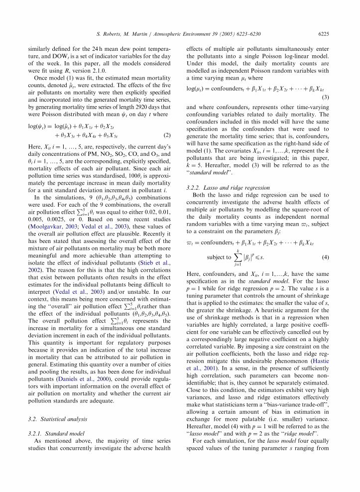
similarly defined for the 24 h mean dew point tempera-

ture, and DOWt is a set of indicator variables for the day

of the week. In this paper, all the models considered

were fit using R, version 2.1.0.

Once model (1) was fit, the estimated mean mortality

counts, denoted m̂t, were extracted. The effects of the five

air pollutants on mortality were then explicitly specified

and incorporated into the generated mortality time series,

by generating mortality time series of length 2920 days that

were Poisson distributed with mean ct on day t where

logðctÞ ¼ logðm̂tÞ þ y1X 1t þ y2X 2t

þ y3X 3t þ y4X 4t þ y5X 5t ð2Þ

Here, Xit i ¼ 1, y, 5, are, respectively, the current day’s

daily concentrations of PM, NO2, SO2, CO, and O3, and

yi i ¼ 1,y, 5, are the corresponding, explicitly specified,

mortality effects of each air pollutant. Since each air

pollution time series was standardised, 100yi is approxi-

mately the percentage increase in mean daily mortality

for a unit standard deviation increment in pollutant i.

In the simulations, 9 (y1,y2,y3,y4,y5) combinations

were used. For each of the 9 combinations, the overall

air pollution effectP5

i¼1yi was equal to either 0.02, 0.01,

0.005, 0.0025, or 0. Based on some recent studies

(Moolgavkar, 2003; Vedal et al., 2003), these values of

the overall air pollution effect are plausible. Recently it

has been stated that assessing the overall effect of the

mixture of air pollutants on mortality may be both more

meaningful and more achievable than attempting to

isolate the effect of individual pollutants (Stieb et al.,

2002). The reason for this is that the high correlations

that exist between pollutants often results in the effect

estimates for the individual pollutants being difficult to

interpret (Vedal et al., 2003) and/or unstable. In our

context, this means being more concerned with estimat-

ing the ‘‘overall’’ air pollution effectP5

i¼1yirather than

the effect of the individual pollutants (y1,y2,y3,y4,y5).The overall pollution effect

P5i¼1yi represents the

increase in mortality for a simultaneous one standard

deviation increment in each of the individual pollutants.

This quantity is important for regulatory purposes

because it provides an indication of the total increase

in mortality that can be attributed to air pollution in

general. Estimating this quantity over a number of cities

and pooling the results, as has been done for individual

pollutants (Daniels et al., 2000), could provide regula-

tors with important information on the overall effect of

air pollution on mortality and whether the current air

pollution standards are adequate.

3.2. Statistical analysis

3.2.1. Standard model

As mentioned above, the majority of time series

studies that concurrently investigate the adverse health

effects of multiple air pollutants simultaneously enter

the pollutants into a single Poisson log-linear model.

Under this model, the daily mortality counts are

modelled as independent Poisson random variables with

a time varying mean mt where

logðmtÞ ¼ confounderst þ b1X 1t þ b2X 2t þ � � � þ bkX kt

(3)

and where confounderst represents other time-varying

confounding variables related to daily mortality. The

confounders included in this model will have the same

specification as the confounders that were used to

generate the mortality time series; that is, confounderst

will have the same specification as the right-hand side of

model (1). The covariates Xit, i ¼ 1,y,k, represent the k

pollutants that are being investigated; in this paper,

k ¼ 5. Hereafter, model (3) will be referred to as the

‘‘standard model’’.

3.2.2. Lasso and ridge regression

Both the lasso and ridge regression can be used to

concurrently investigate the adverse health effects of

multiple air pollutants by modelling the square-root of

the daily mortality counts as independent normal

random variables with a time varying mean $t, subject

to a constraint on the parameters bj:

$t ¼ confounderst þ b1X 1t þ b2X 2t þ � � � þ bkX kt

subject toXk

j¼1

bj

�� ��pps. ð4Þ

Here, confounderst and Xit, i ¼ 1,y,k, have the same

specification as in the standard model. For the lasso

p ¼ 1 while for ridge regression p ¼ 2. The value s is a

tuning parameter that controls the amount of shrinkage

that is applied to the estimates: the smaller the value of s,

the greater the shrinkage. A heuristic argument for the

use of shrinkage methods is that in a regression when

variables are highly correlated, a large positive coeffi-

cient for one variable can be effectively cancelled out by

a correspondingly large negative coefficient on a highly

correlated variable. By imposing a size constraint on the

air pollution coefficients, both the lasso and ridge reg-

ression mitigate this undesirable phenomenon (Hastie

et al., 2001). In a sense, in the presence of sufficiently

high correlation, such parameters can become non-

identifiable; that is, they cannot be separately estimated.

Close to this condition, the estimators exhibit very high

variances, and lasso and ridge estimators effectively

make what statisticians term a ‘‘bias-variance trade-off’’,

allowing a certain amount of bias in estimation in

exchange for more palatable (i.e. smaller) variance.

Hereafter, model (4) with p ¼ 1 will be referred to as the

‘‘lasso model’’ and with p ¼ 2 as the ‘‘ridge model’’.

For each simulation, for the lasso model four equally

spaced values of the tuning parameter s ranging from

ARTICLE IN PRESSS. Roberts, M. Martin / Atmospheric Environment 39 (2005) 6223–62306226

0:85P5

j¼1 b̂j

������ to

P5j¼1 b̂j

������, inclusive were considered,

where b̂j are the parameter estimates obtained from

model (4) with no constraints placed on the coefficients.

This range of s values was based on an initial

exploratory analysis which suggested that smaller values

of s resulted in too much shrinkage and the fact that

values of sXP5

j¼1 b̂j

������ result in identical estimates being

obtained. For each simulation, the value of s within this

range that was used to obtain the estimates was based on

a test data set of length 365 days—the last 365 days of

each of the generated mortality time series was set-aside

and the s value that was ‘‘best’’ able to predict the 365

days of set-aside mortality was selected. For each

simulation, for the ridge model four values of the tuning

parameter s were also considered. The four values

considered corresponded to a similar level of shrinkage

as used in the lasso model. As for the lasso model, the s

value used to obtain the estimates was based on a test

data set of length 365 days. It is important to reiterate

that for each simulation that was run (i.e., for each

generated mortality time series) the procedures de-

scribed above were used to estimate two new values of

the tuning parameter s—one for the lasso model and one

for the ridge model. The estimation of the tuning

parameters was an explicit part of both the lasso and

ridge models estimation procedures.

The standard model was implemented using Poisson

log-linear regression based on the daily mortality counts,

while both the lasso and ridge models were implemented

using normal linear regression based on the square-root

of the daily mortality counts. The reason for this choice

is that the lasso and ridge regression were originally

developed in the context of the normal linear regression

framework. Previous studies have shown that for our

purposes Poisson log-linear regression and normal linear

regression with a square-root transformation lead to

similar results (Smith et al., 2000).

3.2.3. Criteria for evaluation

For each of the 9 (y1,y2,y3,y4,y5) combinations, 1000mortality time series were generated using model (2).

For each generated mortality time series, the individual

pollutant effects (y1,y2,y3,y4,y5) and the overall air

pollution effectP5

i¼1yi were estimated using the

standard, lasso and ridge models. For each set of 1000

simulations, the root mean squared error (rmse),

standard deviation, and bias of the estimates obtained

from each of the three models was calculated. The rmse

is a standard method of comparing estimators or models

that provides a measure of accuracy that incorporates

both bias and variance. Smaller rmse values correspond

to better estimators in the sense of having both relatively

small bias and small variance. The results of the

simulations are reported in Tables 1 and 2.

4. Results

Table 1 contains the results of the simulations for

mortality generated with each pollutant having either no

effect on mortality or each pollutant having an effect on

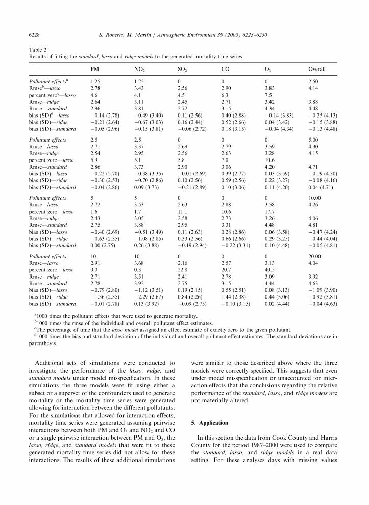
mortality. Table 2 contains the results of the simulations

for mortality generated with PM and NO2 having an

effect on mortality and SO2, CO, and O3 having no

effect on mortality. These tables contain the rmse, bias,

and standard deviation of the estimates obtained from

the standard, lasso, and ridge models.

In both tables the rmse values for the estimates

obtained from both the lasso and ridge models are

generally smaller than the rmse values for the estimates

obtained from the standard model. This indicates that

both the lasso and ridge models provide more accurate

estimates of both the effect of the individual pollutants

on mortality and of the overall effect of air pollution on

mortality than the standard model. The increase in

accuracy can sometimes be substantial. For example, in

simulation 9 the rmse value of the estimate obtained for

the effect of O3 on mortality from the lasso model was

30% smaller than the corresponding estimate obtained

from the standard model.

As discussed above, the increased accuracy of the

estimates obtained from both the lasso and ridge models

is due to a ‘‘bias-variance trade-off’’. From Tables 1 and

2, it can be seen that the individual pollutant effect

estimates obtained from both the lasso and ridge models

have a larger bias than the estimates obtained from the

standard model. This bias becomes material in simula-

tion 9 when PM and NO2 have a large effect on

mortality and SO2, CO, and O3 have no effect on

mortality. However, importantly, it can also be seen that

the overall pollution effect estimates obtained from the

both the lasso and ridge models do not have a material

bias. The increased bias of the estimates obtained from

both the lasso and ridge models is typically more than

compensated for by a reduction in variance, as

illustrated by the increased accuracy of the estimates

obtained from both the lasso and ridge models compared

to the standard model. The lasso model did not perform

well when large values of the overall effect of air

pollution on mortality were used, most notably simula-

tion 5. In this case, the bias component of the rmse rose

significantly for the lasso model. Statistically, the reason

for this phenomenon is that shrinkage is largest when

the effects are large resulting in the large increase in the

negative bias of the estimates from the lasso model.

The lasso model has one important advantage over

both the ridge and standard models. The nature of the

constraint on the coefficients in the lasso means that it

can return parameter estimates of exactly zero (Tibshir-

ani, 1996). In our context, this means that the lasso

model will sometimes return air pollutant effect esti-

mates of exactly zero; this will never be the case for both

ARTICLE IN PRESS

Table 1

Results of fitting the standard, lasso and ridge models to the generated mortality time series

PM NO2 SO2 CO O3 Overall

Pollutant effectsa 0 0 0 0 0 0

Rmseb—lasso 2.61 3.56 2.83 2.95 3.86 4.50

rmse—ridge 2.49 3.30 2.70 2.79 3.55 4.31

rmse—standard 2.78 3.90 2.95 3.17 4.28 4.83

Bias (SD)c—lasso 0.01 (2.61) �0.38 (3.54) 0.06 (2.83) 0.27 (2.94) 0.02 (3.86) �0.02 (4.50)

Bias (SD)—ridge 0.01 (2.50) �0.53 (3.26) 0.10 (2.70) 0.36 (2.77) 0.15 (3.55) 0.09 (4.31)

Bias (SD)—standard 0.05 (2.78) �0.14 (3.90) �0.08 (2.95) 0.11 (3.17) 0.12 (4.28) 0.07 (4.83)

Pollutant effects 0.50 0.50 0.50 0.50 0.50 2.50

rmse—lasso 2.63 3.53 2.78 2.96 3.89 4.50

rmse—ridge 2.54 3.21 2.66 2.77 3.56 4.29

rmse—standard 2.78 3.88 2.91 3.21 4.40 4.84

Bias (SD)—lasso �0.15 (2.63) �0.30 (3.52) 0.11 (2.78) 0.15 (2.96) �0.16 (3.89) �0.36 (4.49)

Bias (SD)—ridge �0.16 (2.53) �0.42 (3.18) 0.14 (2.65) 0.21 (2.76) �0.09 (3.56) �0.32 (4.28)

Bias (SD)—standard �0.09 (2.78) �0.02 (3.88) �0.02 (2.91) �0.04 (3.21) �0.01 (4.40) �0.18 (4.84)

Pollutant effects 1.00 1.00 1.00 1.00 1.00 5.00

rmse—lasso 2.61 3.48 2.72 2.84 3.81 4.41

rmse—ridge 2.49 3.12 2.60 2.65 3.52 4.25

rmse—standard 2.79 3.84 2.87 3.09 4.35 4.75

Bias (SD)—lasso �0.01 (2.61) �0.16 (3.48) �0.05 (2.73) 0.16 (2.83) �0.27 (3.80) �0.34 (4.40)

Bias (SD)—ridge �0.02 (2.49) �0.30 (3.10) �0.01 (2.60) 0.24 (2.64) �0.24 (3.51) �0.33 (4.24)

Bias (SD)—standard 0.08 (2.79) 0.14 (3.84) �0.19 (2.87) �0.02 (3.09) �0.09 (4.35) �0.07 (4.75)

Pollutant effects 2.00 2.00 2.00 2.00 2.00 10.00

rmse—lasso 2.70 3.68 2.70 2.97 3.74 4.11

rmse—ridge 2.58 3.36 2.59 2.83 3.63 4.11

rmse—standard 2.87 3.95 2.83 3.20 4.37 4.55

Bias (SD)—lasso �0.11 (2.70) �0.52 (3.64) 0.03 (2.70) 0.37 (2.95) �0.20 (3.74) �0.42 (4.09)

Bias (SD)—ridge �0.08 (2.58) �0.63 (3.30) 0.08 (2.59) 0.46 (2.79) �0.23 (3.63) �0.40 (4.09)

Bias (SD)—standard 0.07 (2.87) �0.23 (3.95) �0.04 (2.83) 0.22 (3.19) 0.19 (4.37) 0.20 (4.54)

Pollutant effects 4.00 4.00 4.00 4.00 4.00 20.00

rmse—lasso 2.70 3.57 2.81 2.99 3.95 5.06

rmse—ridge 2.50 3.13 2.65 2.75 3.80 4.58

rmse—standard 2.77 3.78 2.90 3.15 4.33 4.69

Bias (SD)—lasso �0.43 (2.67) �0.23 (3.57) �0.13 (2.81) �0.08 (2.99) �0.86 (3.86) �1.73 (4.76)

Bias (SD)—ridge �0.21 (2.49) �0.45 (3.10) 0.05 (2.65) 0.16 (2.75) �0.69 (3.74) �1.14 (4.44)

Bias (SD)—standard 0.03 (2.77) 0.06 (3.78) �0.01 (2.90) �0.16 (3.15) 0.04 (4.33) �0.04 (4.69)

a1000 times the pollutant effects that were used to generate mortality.b1000 times the rmse of the individual and overall pollutant effect estimates.c1000 times the bias and standard deviation of the individual and overall pollutant effect estimates. The standard deviations are in

parentheses.

S. Roberts, M. Martin / Atmospheric Environment 39 (2005) 6223–6230 6227

the ridge and standard models. Table 2 contains the

percentage of times in each set of 1000 simulations that

the lasso model returned an effect estimate of exactly

zero for each pollutant in simulations 6–9. From this

table it can be seen that in simulation 9, the lasso model

assigns estimates of zero a large percentage of the time

to the three pollutants with a zero mortality effect, but

apart from this the percentage of zero estimates assigned

to these three pollutants is quite small. Smaller values of

the tuning parameter s would result in a higher

percentage of zero estimates at the expense of further

increased bias. The ability of the lasso model to return

estimates of exactly zero is important because it may lead

to more interpretable models than those obtained from

both the ridge and standard models. This feature is

particularly important given that researchers have

recently concluded that pollutants measured and included

in models of daily mortality might better be interpreted as

indicators of the biologically relevant pollutant mixture

(Moolgavkar, 2003; Venners et al., 2003). The lasso model

with its ability to assign air pollutant effect estimates of

exactly zero clearly fits better into this paradigm, because

it allows for particular pollutant coefficients to be

eliminated completely during the modelling process.

ARTICLE IN PRESS

Table 2

Results of fitting the standard, lasso and ridge models to the generated mortality time series

PM NO2 SO2 CO O3 Overall

Pollutant effectsa 1.25 1.25 0 0 0 2.50

Rmseb—lasso 2.78 3.43 2.56 2.90 3.83 4.14

percent zeroc—lasso 4.6 4.1 4.5 6.3 7.5

Rmse—ridge 2.64 3.11 2.45 2.71 3.42 3.88

Rmse—standard 2.96 3.81 2.72 3.15 4.34 4.48

bias (SD)d—lasso �0.14 (2.78) �0.49 (3.40) 0.11 (2.56) 0.40 (2.88) �0.14 (3.83) �0.25 (4.13)

bias (SD)—ridge �0.21 (2.64) �0.67 (3.03) 0.16 (2.44) 0.52 (2.66) 0.04 (3.42) �0.15 (3.88)

bias (SD)—standard �0.05 (2.96) �0.15 (3.81) �0.06 (2.72) 0.18 (3.15) �0.04 (4.34) �0.13 (4.48)

Pollutant effects 2.5 2.5 0 0 0 5.00

Rmse—lasso 2.71 3.37 2.69 2.79 3.59 4.30

Rmse—ridge 2.54 2.95 2.56 2.63 3.28 4.15

percent zero—lasso 5.9 5.1 5.8 7.0 10.6

Rmse—standard 2.86 3.73 2.90 3.06 4.20 4.71

bias (SD)—lasso �0.22 (2.70) �0.38 (3.35) �0.01 (2.69) 0.39 (2.77) 0.03 (3.59) �0.19 (4.30)

bias (SD)—ridge �0.30 (2.53) �0.70 (2.86) 0.10 (2.56) 0.59 (2.56) 0.22 (3.27) �0.08 (4.16)

bias (SD)—standard �0.04 (2.86) 0.09 (3.73) �0.21 (2.89) 0.10 (3.06) 0.11 (4.20) 0.04 (4.71)

Pollutant effects 5 5 0 0 0 10.00

Rmse—lasso 2.72 3.53 2.63 2.88 3.58 4.26

percent zero—lasso 1.6 1.7 11.1 10.6 17.7

Rmse—ridge 2.43 3.05 2.58 2.73 3.26 4.06

Rmse—standard 2.75 3.88 2.95 3.31 4.48 4.81

bias (SD)—lasso �0.40 (2.69) �0.51 (3.49) 0.11 (2.63) 0.28 (2.86) 0.06 (3.58) �0.47 (4.24)

bias (SD)—ridge �0.63 (2.35) �1.08 (2.85) 0.33 (2.56) 0.66 (2.66) 0.29 (3.25) �0.44 (4.04)

bias (SD)—standard 0.00 (2.75) 0.26 (3.88) �0.19 (2.94) �0.22 (3.31) 0.10 (4.48) �0.05 (4.81)

Pollutant effects 10 10 0 0 0 20.00

Rmse—lasso 2.91 3.68 2.16 2.57 3.13 4.04

percent zero—lasso 0.0 0.3 22.8 20.7 40.5

Rmse—ridge 2.71 3.51 2.41 2.78 3.09 3.92

Rmse—standard 2.78 3.92 2.75 3.15 4.44 4.63

bias (SD)—lasso �0.79 (2.80) �1.12 (3.51) 0.19 (2.15) 0.55 (2.51) 0.08 (3.13) �1.09 (3.90)

bias (SD)—ridge �1.36 (2.35) �2.29 (2.67) 0.84 (2.26) 1.44 (2.38) 0.44 (3.06) �0.92 (3.81)

bias (SD)—standard �0.01 (2.78) 0.13 (3.92) �0.09 (2.75) �0.10 (3.15) 0.02 (4.44) �0.04 (4.63)

a1000 times the pollutant effects that were used to generate mortality.b1000 times the rmse of the individual and overall pollutant effect estimates.cThe percentage of time that the lasso model assigned an effect estimate of exactly zero to the given pollutant.d1000 times the bias and standard deviation of the individual and overall pollutant effect estimates. The standard deviations are in

parentheses.

S. Roberts, M. Martin / Atmospheric Environment 39 (2005) 6223–62306228

Additional sets of simulations were conducted to

investigate the performance of the lasso, ridge, and

standard models under model misspecification. In these

simulations the three models were fit using either a

subset or a superset of the confounders used to generate

mortality or the mortality time series were generated

allowing for interaction between the different pollutants.

For the simulations that allowed for interaction effects,

mortality time series were generated assuming pairwise

interactions between both PM and O3 and NO2 and CO

or a single pairwise interaction between PM and O3, the

lasso, ridge, and standard models that were fit to these

generated mortality time series did not allow for these

interactions. The results of these additional simulations

were similar to those described above where the three

models were correctly specified. This suggests that even

under model misspecification or unaccounted for inter-

action effects that the conclusions regarding the relative

performance of the standard, lasso, and ridge models are

not materially altered.

5. Application

In this section the data from Cook County and Harris

County for the period 1987–2000 were used to compare

the standard, lasso, and ridge models in a real data

setting. For these analyses days with missing values

ARTICLE IN PRESS

Table 3

Results of applying the lasso, ridge, and standard models to data from Cook County, Illinois and Harris County, Texas for the period

1987–2000

PM NO2 SO2 CO O3 Overalla

Cook County

lassob 0.49 (0.21) 0.00 (0.26) �0.45 (0.24) �0.08 (0.24) 0.00 (0.27) �0.05 (0.34)

Ridge 0.53 (0.23) 0.05 (0.33) �0.50 (0.24) �0.14 (0.25) 0.03 (0.31) �0.02 (0.36)

Standard 0.55 (0.23) 0.05 (0.30) �0.47 (0.22) �0.15 (0.24) 0.10 (0.34) 0.07 (0.37)

Harris County

Lasso �0.53 (0.53) �0.12 (0.84) 0.93 (0.58) �0.04 (0.62) 0.00 (0.67) 0.25 (0.80)

ridge �0.43 (0.52) �0.09 (0.73) 0.73 (0.51) �0.07 (0.60) 0.07 (0.56) 0.21 (0.78)

Standard �0.50 (0.60) �0.44 (1.02) 1.03 (0.62) 0.10 (0.73) 0.06 (0.72) 0.25 (0.82)

aThe increase in mortality for a simultaneous one standard deviation increment in the concentration of each pollutant.bThe estimated percentage increase in mortality for a one standard deviation increment in the pollutant. The values in parentheses

are the standard deviations of the estimates.

S. Roberts, M. Martin / Atmospheric Environment 39 (2005) 6223–6230 6229

across any of the variables were removed. This left 4835

days of data for Cook County and 1703 days of data for

Harris County. The form of the standard, lasso, and

ridge models that were fit to the data from each county is

specified in models (3) and (4) above.

Table 3 contains the results of applying the models to

the data from both counties. In both counties the

standard, lasso, and ridge models gave similar results for

the estimates of the effect of the individual pollutants on

mortality and for the overall effect of air pollution on

mortality. The ability of the lasso model to assign air

pollution effect estimates of exactly zero is clearly

illustrated for these two counties with PM and O3

receiving effect estimates of zero in Cook County and O3

receiving an effect estimate of zero in Harris County. As

discussed above, for reasons of interpretability and the

current interest in biologically relevant pollutant mix-

tures, the ability of the lasso model to assign zero effect

estimates is an important attribute that is not shared by

either the standard or ridge models.

6. Discussion

The results of our study demonstrate that both the

lasso and ridge regression can be used to provide more

accurate estimates of both the individual and overall

mortality effects of multiple air pollutants compared to

the standard method of using a Poisson log-linear

model. However, for estimating the mortality effect of

individual pollutants the increased accuracy of both the

lasso and ridge regression sometimes comes at the

expense of larger bias. This fact should be kept in mind

when these shrinkage methods are used to estimate the

adverse health effects of multiple pollutants.

The study also showed that the more accurate

estimates of the overall air pollution effect obtained

from both the lasso and ridge regression compared to

the standard Poisson log-linear model, came without

the introduction of material bias. This is important

information because it has recently been stated that

assessing the overall effect of the mixture of air

pollutants on mortality may be more meaningful than

assessing the effect of individual pollutants. This study

shows that for this purpose ridge regression should be

preferred to both the lasso and the standard Poisson log-

linear model.

Some other studies have also looked at alternative

models for investigating the adverse health effects of

multiple pollutants. Wong et al. (2002) adopted a

pairwise approach. If more than one pollutant seemed

to be associated with the outcome, the association with

one pollutant stratified by the level of the other pollutant

was sought. Hong et al. (1999) used a number of a priori

fixed air pollution indices to evaluate the combined

effects of various air pollutants. These models differ

from the standard, lasso, and ridge models investigated in

this paper. Unlike these three models which provide

individual effect estimates for each pollutant of interest,

the approach of Wong et al. will only provide estimates

for a subset of two of these five pollutants and the

approach of Hong et al. will only provide an estimate for

an a priori fixed air pollution index on mortality. Since

the approaches of Wong et al. and Hong et al. do not

provide individual effect estimates for each of the five

pollutants considered in this paper they were not

compared here to the standard, lasso, and ridge models.

Use of shrinkage methods such as the lasso or ridge

regression offer a flexible way of obtaining more

accurate estimation of pollutant effects than that

provided by the standard approach. This more accurate

estimation is due to the ‘‘bias-variance trade-off’’. The

results presented in this paper should help researchers

investigating the adverse health effects of multiple air

pollutants decide whether shrinkage methods are appro-

priate for their needs.

ARTICLE IN PRESSS. Roberts, M. Martin / Atmospheric Environment 39 (2005) 6223–62306230

References

Chock, D.P., Winkler, S.L., Chen, C., 2000. A study of the

association between daily mortality and ambient air

pollutant concentrations in Pittsburgh, Pennsylvania. Jour-

nal of Air &Waste Management Association 50, 1481–1500.

Cifuentes, L.A., Vega, J., Kopfer, K., Lave, L.B., 2000. Effect

of the fine fraction of particulate matter versus the coarse

mass and other pollutants on daily mortality in Santiago,

Chile. Journal of Air & Waste Management Association 50,

1287–1298.

Cox, L.H., 2000. Statistical issues in the study of air pollution

involving airborne particulate matter. Environmetrics 11,

611–626.

Daniels, M.J., Dominici, F., Samet, J.M., et al., 2000.

Estimating particulate matter-mortality dose–response

curves and threshold levels: an analysis of daily time-series

for the 20 largest US cities. American Journal of Epide-

miology 152, 397–406.

Derriennic, F., Richardson, S., Mollie, A., et al., 1989. Short-

term effects of sulphur dioxide pollution on mortality in two

French cities. International Journal of Epidemiology 18,

186–197.

Dominici, F., Burnett, R.T., 2003. Risk models for particulate

air pollution. Journal of Toxicology and Environmental

Health Part A 66, 1883–1889.

Hales, S., Salmond, C., Town, G.I., et al., 1999. Daily mortality

in relation to weather and air pollution in Christchurch,

New Zealand. Australian and New Zealand Journal of

Public Health 24, 88–91.

Hastie, T., Tibshirani, R., Friedman, J., 2001. The Elements Of

Statistical Learning. Springer, Berlin.

Hastie, T.J., Tibshirani, R.J., 1990. Generalized Additive

Models. Chapman & Hall, London.

Hong, Y.C., Leem, J.H., Ha, E.H., Christiani, D.C., 1999.

PM10 exposure, gaseous pollutants, and daily mortality in

Inchon, South Korea. Environmental Health Perspectives

107, 873–878.

Ito, K., Kinney, P.L., Thurston, G.D., 1995. Variations in PM-

10 concentrations within two metropolitan areas and their

implications for health effects analyses. Inhalation Toxicol-

ogy 7, 735–745.

Lee, J.T., Kim, H., Hong, Y.C., et al., 2000. Air pollution and

daily mortality in seven major cities of Korea, 1991–1997.

Environmental Research 84, 247–254.

McCullagh, P., Nelder, J.A., 1989. Generalized Linear Models.

Chapman & Hall, London.

Moolgavkar, S.H., 2003. Air pollution and daily mortality in

two US counties: season-specific analyses and exposure-

response relationships. Inhalation Toxicology 15, 877–907.

Ostro, B.D., Hurley, S., Lipsett, M.J., 1999. Air pollution and

daily mortality in the Coachella Valley, California: a study

of PM10 dominated by coarse particles. Environmental

Research 81, 231–238.

Rahlenbeck, S.I., Kahl, H., 1996. Air population and mortality

in East Berlin during the winters of 1981–1989. Interna-

tional Journal of Epidemiology 25, 1220–1226.

Roberts, S., 2004. Interactions between particulate air pollution

and temperature in air pollution mortality time series

studies. Environmental Research 96, 328–337.

Roberts, S., 2005. An investigation of distributed lag models in

the context of air pollution and mortality time series

analysis. Journal of Air & Waste Management Association

55, 273–282.

Smith, R.L., Davis, J.M., Sacks, J., et al., 2000. Regression

models for air pollution and daily mortality: analysis of data

from Birmingham, Alabama. Environmetrics 11, 719–743.

Stieb, D.M., Judek, S., Burnett, R.T., 2002. Meta-analysis of

time-series studies of air pollution and mortality: effects of

gases and particles and the influence of cause of death, age,

and season. Journal of Air & Waste Management Associa-

tion 52, 470–484.

Tibshirani, R., 1996. Regression shrinkage and selection via the

lasso. Journal of the Royal Statistical Society B 58, 267–288.

Tze Wai, W, Ka Ming, H, Tai Shing L, et al. 1997. A study of

short-term effects of ambient air pollution on public health.

A consultancy report for Environmental Protection Depart-

ment Hong Kong. Available from: http://www.epd.gov.hk/

epd/english/environmentinhk/air/studyrpts/cuhk97.html.

Accessed January 3, 2005.

Vedal, S., Brauer, M., White, R., et al., 2003. Air pollution and

daily mortality in a city with low levels of pollution.

Environmental Health Perspectives 111, 45–52.

Venners, S.A., Wang, B., Peng, Z., et al., 2003. Particulate

matter, sulfur dioxide, and daily mortality in Chongqing,

China. Environmental Health Perspectives 111, 562–567.

Wong, T.W., Tam, W.S., Yu, T.S., et al., 2002. Associations

between daily mortalities from respiratory and cardiovas-

cular diseases and air pollution in Hong Kong, China.

Occupational and Environmental Medicine 59, 30–35.

Yang, C.Y., Chen, Y.S., Yang, C.H., et al., 2004. Relationship

between ambient air pollution and hospital admissions for

cardiovascular diseases in Kaohsiung, Taiwan. Journal of

Toxicology and Environmental Health Part A 67, 483–493.