A Continuous Optimization Approach toProtein Design with Structural and

Functional Constraints

A Thesis

Submitted for the Degree of

Doctor of Philosophy

in the Faculty of Engineering

By

Sourav Rakshit

DEPARTMENT OF MECHANICAL ENGINEERING

INDIAN INSTITUTE OF SCIENCE

BANGALORE - 560 012

INDIA

April 2011

Contents

ii

i

To

The loving memory of

My grandparents

Binapani Rakshit

Sudhir Chandra Rakshit

Padmabati Saha

Sudhir Kumar Saha

ii

Table of Contents Title Page number

Abstract ................................................................................................................. iv

Acknowledgments ................................................................................................. v

List of Figures ...................................................................................................... vii

List of Tables ........................................................................................................ xi

List of Equations .................................................................................................. xii

1. Introduction ........................................................................................................ 1

1.1 Preamble ...................................................................................................... 1

1.2 Proteins ........................................................................................................ 3

1.2.1 A brief overview of protein structure and folding ................................ 3

1.2.2 A brief overview of protein design ...................................................... 8

1.3 Motivation .................................................................................................. 12

1.4 Problem statement ..................................................................................... 14

1.5 Scope of the thesis ..................................................................................... 17

1.6 Organization of the thesis .......................................................................... 18

1.7 Closure ....................................................................................................... 19

2. Literature Review ............................................................................................. 20

2.1 Reduced amino acid alphabet ................................................................... 20

2.2 Computational protein sequence design ................................................... 22

2.3 Elastic networks ....................................................................................... 25

2.4 Minimalist coarse-grained models ........................................................... 28

2.5 Closure ...................................................................................................... 31

3. Reduced Amino Acid Alphabet using Metric Multi-dimensional Scaling ...... 32

3.1 Introduction ............................................................................................... 32

3.2 Method ...................................................................................................... 33

3.3 Results and discussion ............................................................................... 37

3.4 Closure ....................................................................................................... 44

4. Search in the Sequence Space .......................................................................... 45

4.1 Introduction ............................................................................................... 45

4.2 The Double Sigmoid method ..................................................................... 49

iii

4.2.1 Formulation of the continuous optimization problem ........................ 49

4.2.2 Formulation of the constraints ............................................................ 55

4.2.3 Results ................................................................................................ 55

4.3 The Quadratic Programming method ........................................................ 69

4.3.1 Method ............................................................................................... 69

4.3.2 Results ................................................................................................ 71

4.4 Discussion .................................................................................................. 79

4.5 Closure ....................................................................................................... 81

5. Search in the Conformation Space ................................................................... 82

5.1 Introduction ............................................................................................... 82

5.2 Coarse-grained energy function formulation ............................................ 83

5.3 The Elastic Network Model ...................................................................... 88

5.3.1 Method .............................................................................................. 88

5.3.2 Results ................................................................................................ 92

5.3 Secondary structure formation using continuous optimization ................. 98

5.4 Conformation search using coarse-grained model with rigid secondary

structures .................................................................................................. 102

5.4.1 Method ............................................................................................. 102

5.4.2 Results .............................................................................................. 104

5.5 Discussion ................................................................................................ 110

5.6 Closure ..................................................................................................... 111

6. Simultaneous search in the sequence and conformation spaces:

An application ................................................................................................ 112

6.1 Introduction .............................................................................................. 112

6.2 A brief description the target protein: The hen egg-white Lysozyme ..... 115

6.3 Modeling and results ................................................................................ 117

6.4 Discussion ................................................................................................ 127

6.5 Closure ..................................................................................................... 129

7. Towards parallelization of tertiary structure prediction using Graphics

Processor Unit (GPU) based parallel computation ........................................ 130

7.1 Introduction and motivation ..................................................................... 130

iv

7.2 From CPU-based code to GPU-based code ............................................. 133

7.3 A case study with CPU and GPU based codes ........................................ 136

7.4 Closure ..................................................................................................... 141

8. Closure and future work ................................................................................. 142

8.1 Summary and conclusions ....................................................................... 142

8.2 Contributions of the thesis ....................................................................... 145

8.3 Future work ............................................................................................. 146

Appendix A ......................................................................................................... 149

Appendix B ......................................................................................................... 151

B1 Interior Point Optimization (IPOPT) ....................................................... 151

B2 SCWRL .................................................................................................... 152

B3 Nonlinear conjugate gradient method ..................................................... 152

B4 Online Secondary Structure prediction servers ....................................... 154

Appendix C ......................................................................................................... 156

References .......................................................................................................... 164

v

Abstract

We have developed a novel computational approach to functional de novo protein design

using gradient-based continuous optimization techniques. Motivated by many

engineering optimization applications in which a cost function is optimized subject to a

set of constraints, we pose functional protein design task as a continuous optimization

problem to search sequence and conformation spaces simultaneously. The methods used

in sequence-space search are analogous to the material-design formulations in topology

optimization of structures, whereas the conformation search techniques are similar to

mechanical-link like models and modal analysis of structures. Computationally efficient

techniques such as nonlinear conjugate gradient and interior point optimization are used

to solve the optimization problems. Both the sequence and conformation search

techniques are individually validated with real proteins. Coarse-grained as well as

atomistic level potentials are used to model the energy. Finally, we combined the

sequence and conformation search methods and propose a new strategy for simultaneous

search in the sequence and conformation spaces for designing functionalistic de novo

proteins. In view of lack of experimental resources, the proposed computational scheme

is validated by re-designing an existing protein, the hen-egg white lysozyme. Since the

thrust of this work is on developing computationally efficient models, we developed an

amino acid grouping scheme based on metric multi-dimensional scaling. Some structure-

prediction problems are also solved using Graphical Processing Unit (GPU) based

Compute Unified Device Architecture (CUDA) programming.

vi

Acknowledgments

Pursuing a doctorate degree in an interdisciplinary field at IISc has been the most

memorable achievement in my life. Through this experience I have known myself, my

strengths and drawbacks, and have explored territories that I wouldn’t have even thought

of getting into before I came to IISc. Hence, the largest share of my acknowledgment

goes to this Institute, which has not only molded my way of thinking but also my way of

life, my attitude towards life and society, and my character.

Now, turning to mortal beings, I have to do injustice to so many people by not

acknowledging them directly in this short space, who knowingly or unknowingly, have

helped me through this journey. However, the most prominent one who comes in my

mind is my research supervisor, professor G. K. Ananthasuresh, or Suresh as we call him.

Suresh was my research supervisor in M. Tech., and during this period I was

considerably influenced by his way of teaching, his interdisciplinary topics of research,

and of course his stress on good technical writing and presentations. However, it was

only during PhD that I was able to acquire the skills that are so necessary to convey one’s

ideas and works convincingly in a research paper or a presentation, and for that the credit

goes entirely to Suresh. My PhD topic involved subjects which were new to both of us,

and Suresh was always supportive of the new ideas that I thought of working on. During

the course of my PhD, there were both moments of enjoyment and crisis in my family,

and many times I took leaves which were much longer than what his other students used

to take. I am also grateful to him for allowing me to do so.

Due to the interdisciplinary nature of my work, I had to venture in several

subjects which were new to me. Various courses offered in different departments in IISc

were highly helpful to get initiated into unknown topics. Thus, I am indebted to all the

teachers whose classes I attended. Also, I learned many things relevant to my research

from friends in various departments in IISc, and I feel fortunate to be in such an

academic and research oriented community. I feel especially grateful to Mr. Sumanta

Mukherjee in bioinformatics, and frankly speaking, without his help I might not have

been so successful with the work that I have done. Sumanta helped me in installing the

IPOPT software, which I alone was not able to install in my computer, and further helped

vii

in debugging the C++ codes in which I used to get stuck. He taught me perl and other

scripting languages, which were necessary for running batch computations and parsing

operations, and still a part of my work depends on codes entirely written by him as the

work demanded a high level of codemanship which I have not acquired till now. These

were an invaluable service to an unskilled programmer like me. He was also an eager

helper in my efforts in parallelizing my codes and a part of my parallel codes were

actually tested in his cluster. Regarding parallel programming, I must acknowledge the

help of two of my lab mates, Meenakshi and Ganesh.

Biology was a remote subject to me when I started my work, and my last touch

with biology went back to 10th standard. Sumanta, Amit, Kalidas, Anupam and others

helped me to gain a footing in the area of molecular biophysics which was to be the area

of my research. I am also thankful to my friends Narayana, Sangamesh, Soumyakanti,

Pradipta, Pradeep, Nandkumar, Achintya, Indrajeet, and others who were always

available for a discussion on any theoretical and computational issues. I am especially

grateful to my friends Shamik, Anindya, and Deep, who even though were far away from

IISc, were always in touch with me and supportive of my efforts. And I will always be

thankful to all my friends like Kamalesh, Anirban, Arindam, Ranajit, Subhabrata, Anup,

Satadal, and many others who are like a family to me in IISc.

viii

List of Figures

Figure number Page number

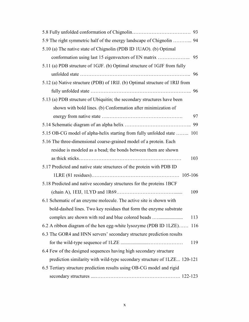
1.1 Analogy between compliant mechanisms and proteins ...………………… 2

1.2 The hierarchic levels of protein structure ………………………………… 5

1.3 Different energy funnels …………………………………………………. 7

1.4 A top view of a four-helix bundle ………………………………………... 8

1.5 The flow diagram of our functional protein design strategy ……………. 15

3.1 Plot of stress against number of dimensions ……………………………. 35

3.2 Scatter diagram showing the discrepancies between entries in the

distance matrix and corresponding distances calculated from the

MMDS map .................................................................................... 36

3.3 MMDS amino acid map constructed using the matrix where we

subtracted diagonal elements from the corresponding rows ....…….. 37

3.4 Amino acid map constructed using the metric multi-dimensional scaling

method and the modified Miyazawa-Jernigan matrix as the proximity

matrix …………………………………………………………………… 37

3.5 Properties of amino acids shown on the MMDS map ………………….. 39

3.6 The residues that have a positive log odd score in the BLOSUM62

matrix are connected by double ended arrows .…………………….. 40

3.7 The residues that have a positive log odd score in the PAM250

matrix are connected by double ended arrows ...…………………… 40

3.8 Dendrogram showing hierarchical grouping of amino acids based

on our distance matrix …………………………………………….. 42

3.9 Minimum distance between groups as a function of the number of

groups …………………………………………………………………… 43

3.10 Grouping of amino acids into five groups based on hierarchical

clustering method…………………………………………............... 44

4.1 Native structure of the four proteins that we target for sequence design.

The number of residues in each protein is also indicated ………………. 46

4.2 In clockwise order from the top ………………………………………… 50

ix

4.3 The double sigmoid function for energy of interaction between all

twenty amino acids …………………………………………………. 52

4.4 Sigmoid function representation of the secondary structure propensities.. 54

4.5 Plot of the constraints. Each colored line is the plot of the constraint ….. 56

4.6 Best designed sequences based on our scoring scheme using

different potentials with and without amino acid composition

constraints for each of the four proteins .………………….. ............. 58-59

4.7 Plots of energy gap ( E native avg decoysE E −∆ = − ) versus Eσ (the standard

deviation of energy of the decoy set structures) …………………….. 63-67

4.8 The highest scoring designed sequences for the four proteins ……… 74-77

4.9 Results of sequence alignment using sequence alignment program

CLUSTAL …………………………………………………………… 77-78

4.10 Plots of energy gap ( E native avg decoysE E −∆ = − ) versus Eσ (the standard

deviation of energy of the decoy set structures) ……………………….. 79

5.1 Variation of contact energy between thi and thj residues ( ijE in kT

units) as a function of distance between them ( ijL in 0A ).…………. 85

5.2 The limits of angle θ between three adjacent Cα atoms ………………. 86

5.3 Variation of bond energy Eθ with angle θ formed by three bonded Cα

atoms ……………………………………………………………………. 87

5.4 Elastic network model of a small de-novo protein, Chignolin ………….. 88

5.5 Flowchart showing our algorithm for large change in conformation

determined using eigenvectors of stiffness matrix K of EN …………… 90

5.6 Energy versus number of iterations for different intervals of

iteration (maxiter) at which optimization program fminunc updates

stiffness matrix of EN ………………………………………………. 91

5.7 Conformation of Chignolin in native state and after optimization.

The left conformation (red lines and blue circles) represent the

native state from PDB…………………………………………......... 92

x

5.8 Fully unfolded conformation of Chignolin……………………………… 93

5.9 The right symmetric half of the energy landscape of Chignolin ………... 94

5.10 (a) The native state of Chignolin (PDB ID 1UAO). (b) Optimal

conformation using last 15 eigenvectors of EN matrix ……………….. 95

5.11 (a) PDB structure of 1GJF. (b) Optimal structure of 1GJF from fully

unfolded state ………………………………………………………….. 96

5.12 (a) Native structure (PDB) of 1RIJ. (b) Optimal structure of 1RIJ from

fully unfolded state …………………………………………………….. 96

5.13 (a) PDB structure of Ubiquitin; the secondary structures have been

shown with bold lines. (b) Conformation after minimization of

energy from native state ….………………………………………. 97

5.14 Schematic diagram of an alpha helix ………………………………….. 99

5.15 OB-CG model of alpha-helix starting from fully unfolded state …….. 101

5.16 The three-dimensional coarse-grained model of a protein. Each

residue is modeled as a bead; the bonds between them are shown

as thick sticks……………………………………………………… 103

5.17 Predicted and native state structures of the protein with PDB ID

1LRE (81 residues)……………………………………………… 105-106

5.18 Predicted and native secondary structures for the proteins 1BCF

(chain A), 1EIJ, 1LYD and 1R69………………………………...... 109

6.1 Schematic of an enzyme molecule. The active site is shown with

bold-dashed lines. Two key residues that form the enzyme substrate

complex are shown with red and blue colored beads .….................... 113

6.2 A ribbon diagram of the hen egg-white lysozyme (PDB ID 1LZE)…… 116

6.3 The GOR4 and HNN servers’ secondary structure prediction results

for the wild-type sequence of 1LZE .......................………………… 119

6.4 Few of the designed sequences having high secondary structure

prediction similarity with wild-type secondary structure of 1LZE... 120-121

6.5 Tertiary structure prediction results using OB-CG model and rigid

secondary structures ....……………………………………………. 122-123

xi

6.6 Plots of energy gap ( E target structure avg decoysE E− −∆ = − ) versus Eσ (the

standard deviation of energy of the decoy set structures) for the

designed sequences..………………………………………………… 126

7.1 The logic of CPU and GPU based codes ……………………………… 132

7.2 Flow diagram of tertiary structure prediction code …………………… 133

7.3 Flowchart of the algorithm evalE_dEdx …………………………. 135-136

7.4 The function value and norm of the gradient of the same for

evalE_dEdx for the CPU and GPU codes ………………............. 139-140

xii

List of Tables

Table number Page number

4.1 Number of matches of the best designed sequences given in Fig.

4.6 using different grouping schemes for each of the four proteins

using all three types of potentials ………………………………….. 60-62

4.2 Average time taken for designing sequences of each protein using

MJ (Miyazawa and Jernigan, 1996), ZSk (Zhang and Skolnick,

1998) and atomistic potentials (Cornell at al., 1995, Fraternali and

Gunsteren, 1996)………………………………………………….... 69

4.3 Average time taken to design sequences for each protein in the FISA

decoy set using quadratic programming formulation ………………….. 72

5.1 Table showing number of iterations required by the optimization

program fminunc to converge as the stiffness matrix of K is

updated after a particular number of iterations for Chignolin …….. 91

5.2 Protein structure prediction results using nonlinear conjugate

gradient algorithm. The first column shows the PDB id. of the

protein, the number of residues in it, and the percentage of residues

in secondary structures (α -helices)……………………………..... 107-108

5.3 Results of ab initio structure prediction with secondary structures

predicted by the HNN server ..…………………………………... 110

6.1 Few selected examples of tertiary structure prediction results using

both energy models. Under each energy model, the first column

indicates the DRMSD of the unfolded conformation from 1LZE

(C α− coordinates only) which serves as input to optimization

program……………………………………………………….…... 124

7.1 Time required for different calculations in the function

evalE_dEdx in CPU and GPU. The calculations are named

similarly as they are presented in Fig. 7.3. ……………………....... 137

xiii

List of Equations

Equation number Page number

1.1…………………………………………………………………………….. 14

1.2…………………………………………………………………………….. 16

3.1…………………………………………………………………………….. 34

3.2…………………………………………………………………………….. 34

3.3…………………………………………………………………………….. 34

3.4…………………………………………………………………………….. 35

3.5…………………………………………………………………………….. 35

4.1…………………………………………………………………………….. 50

4.2…………………………………………………………………………….. 51

4.3…………………………………………………………………………….. 51

4.4…………………………………………………………………………….. 51

4.5…………………………………………………………………………….. 51

4.6…………………………………………………………………………….. 53

4.7…………………………………………………………………………….. 53

4.8…………………………………………………………………………….. 53

4.9…………………………………………………………………………….. 53

4.10…………………………………………………………………………… 53

4.11…………………………………………………………………………… 55

4.12…………………………………………………………………………… 55

4.13…………………………………………………………………………… 62

4.14…………………………………………………………………………… 69

4.15…………………………………………………………………………… 69

4.16…………………………………………………………………………… 70

4.17…………………………………………………………………………… 70

4.18…………………………………………………………………………… 71

4.19…………………………………………………………………………… 71

4.20…………………………………………………………………………… 78

5.1…………………………………………………………………………….. 84

xiv

5.2…………………………………………………………………………….. 85

5.3…………………………………………………………………………….. 86

5.4…………………………………………………………………………….. 87

5.5…………………………………………………………………………….. 87

5.6…………………………………………………………………………….. 89

5.7…………………………………………………………………………….. 99

5.8…………………………………………………………………………… 102

5.9…………………………………………………………………………… 103

5.10………………………………………………………………………….. 104

6.1…………………………………………………………………………… 118

6.2…………………………………………………………………………… 118

1

1. Introduction

• A preamble to the thesis is given.

• Brief reviews of protein structure and folding are presented.

• Brief review of protein design is given.

• The motivation for the work is described.

• Protein design is posed as an optimization problem.

• The scope of the thesis is noted.

• The organization of the thesis is described.

• The chapter is closed with a brief summary.

1.1 Preamble

This thesis presents work on computational design of protein molecules for structural and

functional specifications using gradient-based optimization. Proteins are molecular

machines that perform life-sustaining functions, for example, decoding genetic

information, catalyzing bio-chemical reactions, triggering immune response, sustaining

rigidity and shape of cells and tissues, facilitating chemical signaling among cells, etc.

(Brandon and Tooze, 2001). The sequence of amino acids along a protein’s linear chain

determines its folded structure, also called the conformation, which is crucial to its

specific function. Thus, the protein design problem entails the determination of the amino

acid sequence so that it folds into a suitable 3D structure to serve a desired function.

Optimization is inherent in protein design because a protein chain folds into a native

conformation that, reportedly, has the minimum free energy (Anfinsen, 1961, 1973) with

respect to other conformations.

This work is motivated by the broad principles that underlie optimal design of

machines and structures, and compliant mechanisms in particular. Compliant

mechanisms are elastically deformable structures (Howell, 2001). Figure 1 depicts the

analogy between proteins and compliant mechanisms. Both need specific structural forms

to perform their function and change their shape to do it. Just as a protein’s structure and

function are determined by its sequence of amino acids, a compliant mechanism’s

function is decided by its geometry and material. The deformed configuration of a

2

compliant mechanism is governed by the principle of minimum potential energy

analogous to the principle of minimum free energy of a protein obeys while folding. By

Fig. 1.1 Analogy between compliant mechanisms and proteins.

a) A compliant mechanism (a gripper) in the open position.

b) The same gripper in the closed position.

c) A protein (hexokinase) in its non-active (open) position (Adapted from Nelson

and Cox, 2008).

d) The same protein in its active (closed) position. The active site is encircled in the

figure(Adapted from Nelson and Cox, 2008).

(c)

Active site

(d)

(a)

(b)

3

taking advantage of the analogy between proteins and compliant mechanisms and

computationally efficient optimal design techniques developed for compliant mechanisms

and mechanical structures, this thesis adopts a new approach to computational protein

design. We pose de novo protein design (i.e., designing a protein anew) as an

optimization problem wherein the site of action of the protein is specified in terms of its

structure and amino acids as illustrated in Fig. 1.1.

The aspects of protein design considered in the thesis include: (i) reduced amino

acid alphabet that simplifies protein sequences, (ii) search in the sequence space using

continuous modeling, (iii) search in structure space using coarse-grained energy

potentials, and (iv) simultaneous search in sequence and structure spaces using coarse-

grained potentials as well as fine-grained atomistic potentials. While the design

philosophy of the thesis is general and independent of the potentials, we do consider

instances of real proteins to illustrate the efficacy of the proposed methodology.

Before explaining the specific motivation and the scope of the thesis, requisite

background to the different aspects of the work is provided next.

1.2 Proteins

1.2.1 A brief overview of protein structure and folding

Proteins are biopolymer chains made of monomers called amino acid residues (see

Appendix A). They constitute an important class of biomolecules which take part in all

life-sustaining processes. Proteins are the most versatile biomolecules in terms of the

functions they perform. A few activities in which proteins take active part are:

deoxyribonucleic acid (DNA) duplication, DNA to ribonucleic acid (RNA) transcription,

mediating biomolecular reactions, biosignalling, cytoskeleton generation, bioenergetics,

etc. The diverse functions that proteins are able to perform are due to their structure, i.e.,

spatial conformation. This has been possible because proteins differ from other

biopolymers in one significant aspect; unlike other polymers whose molecules exist in

randomly coiled (glassy) state under normal conditions of temperature, chemical and

other environmental conditions (such as those that exist on our planet), molecules of a

particular protein under most of these conditions have a remarkable similarity in

structure. Thus, all molecules of hemoglobin in our red blood cells have a particular

4

structure when they are transporting oxygen, and a slightly different structure when they

are transporting carbon-dioxide.

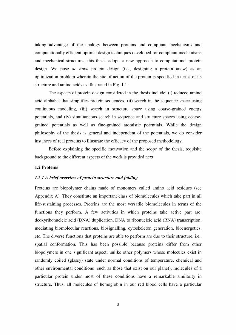
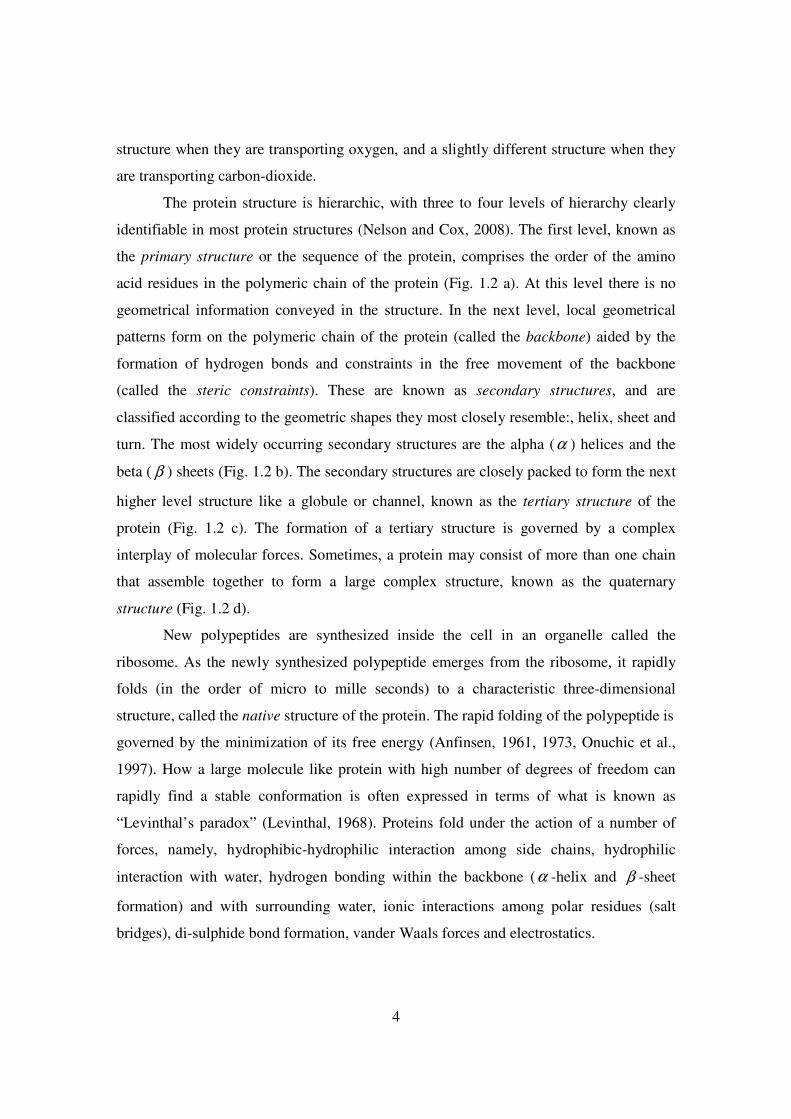
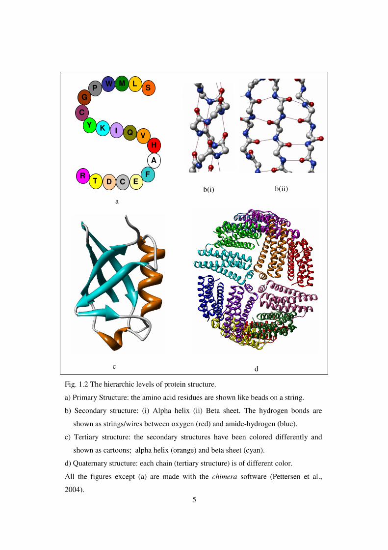
The protein structure is hierarchic, with three to four levels of hierarchy clearly

identifiable in most protein structures (Nelson and Cox, 2008). The first level, known as

the primary structure or the sequence of the protein, comprises the order of the amino

acid residues in the polymeric chain of the protein (Fig. 1.2 a). At this level there is no

geometrical information conveyed in the structure. In the next level, local geometrical

patterns form on the polymeric chain of the protein (called the backbone) aided by the

formation of hydrogen bonds and constraints in the free movement of the backbone

(called the steric constraints). These are known as secondary structures, and are

classified according to the geometric shapes they most closely resemble:, helix, sheet and

turn. The most widely occurring secondary structures are the alpha (α ) helices and the

beta ( β ) sheets (Fig. 1.2 b). The secondary structures are closely packed to form the next

higher level structure like a globule or channel, known as the tertiary structure of the

protein (Fig. 1.2 c). The formation of a tertiary structure is governed by a complex

interplay of molecular forces. Sometimes, a protein may consist of more than one chain

that assemble together to form a large complex structure, known as the quaternary

structure (Fig. 1.2 d).

New polypeptides are synthesized inside the cell in an organelle called the

ribosome. As the newly synthesized polypeptide emerges from the ribosome, it rapidly

folds (in the order of micro to mille seconds) to a characteristic three-dimensional

structure, called the native structure of the protein. The rapid folding of the polypeptide is

governed by the minimization of its free energy (Anfinsen, 1961, 1973, Onuchic et al.,

1997). How a large molecule like protein with high number of degrees of freedom can

rapidly find a stable conformation is often expressed in terms of what is known as

“Levinthal’s paradox” (Levinthal, 1968). Proteins fold under the action of a number of

forces, namely, hydrophibic-hydrophilic interaction among side chains, hydrophilic

interaction with water, hydrogen bonding within the backbone (α -helix and β -sheet

formation) and with surrounding water, ionic interactions among polar residues (salt

bridges), di-sulphide bond formation, vander Waals forces and electrostatics.

5

b(i) b(ii)

c d

Fig. 1.2 The hierarchic levels of protein structure.

a) Primary Structure: the amino acid residues are shown like beads on a string.

b) Secondary structure: (i) Alpha helix (ii) Beta sheet. The hydrogen bonds are

shown as strings/wires between oxygen (red) and amide-hydrogen (blue).

c) Tertiary structure: the secondary structures have been colored differently and

shown as cartoons; alpha helix (orange) and beta sheet (cyan).

d) Quaternary structure: each chain (tertiary structure) is of different color.

All the figures except (a) are made with the chimera software (Pettersen et al.,

2004).

M

G P

W L

I

A

T C

C

F

V

Y

R

H

Q

S

D E

K

a

6

However, recent views substantiated by atomic level experiments and extensive computer

simulations hold that the favorable increase in entropy, which occurs when hydrophobic

residues are packed in the interior of the protein starts the initial folding process (known

as the “hydrophobic collapse”); subsequently the initial folded state, also known as the

“molten globule” is stabilized by the formation of secondary structures, di-sulphide bonds

and ionic interactions among polar residues (Dill, 1990, Nelson and Cox, 2008). The

recent view of protein folding is explained in terms of “the energy landscape” or the

“folding funnel” (Wolynes, 2004). “The new perspective sees folding as a diffusion-like

process, where the motions of individual chains are asynchronous, each being buffeted by

Brownian forces through different sequences of chain conformations, which ultimately

all find their ways to the same native structure, in the same way that water flowing along

different routes down mountainsides can ultimately reach the same lake at the

bottom…..Since the lateral area of an energy landscape at a given depth represents the

number of conformations having the given intra-chain free energy, the funnel idea is

simply that as a folding chain progresses towards lower intra-chain free energies—by

increasing compactness, hydrophobic core development, intra-chain hydrogen bonding,

salt-bridge formation, and so forth—the chain’s conformational options become

increasingly narrowed, ultimately towards one native structure.” (Dill and Chan, 1997).

The different energy landscapes for explaining different observations of protein folding

have been shown in Fig. 1.3. Even though the theoretical framework of protein folding

has been satisfactorily explained based on energy-landscapes, computationally folding a

polypeptide from the conformation when it is released from the ribosome to the native

state is still a daunting task.

7

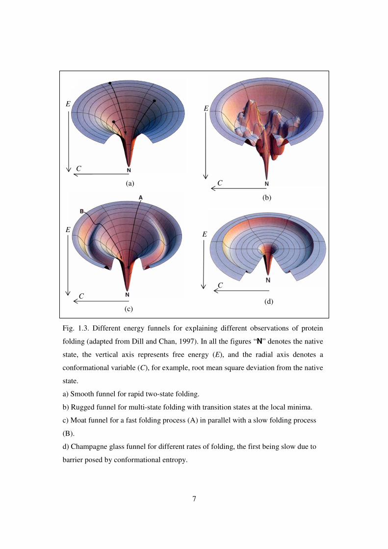
Fig. 1.3. Different energy funnels for explaining different observations of protein

folding (adapted from Dill and Chan, 1997). In all the figures “N” denotes the native

state, the vertical axis represents free energy (E), and the radial axis denotes a

conformational variable (C), for example, root mean square deviation from the native

state.

a) Smooth funnel for rapid two-state folding.

b) Rugged funnel for multi-state folding with transition states at the local minima.

c) Moat funnel for a fast folding process (A) in parallel with a slow folding process

(B).

d) Champagne glass funnel for different rates of folding, the first being slow due to

barrier posed by conformational entropy.

(a)

E

C

(b)

E

C

(c)

E

C (d)

E

C

8

1.2.2 A brief overview of protein design

There are two goals of protein design. The first is to design proteins from the first

principles, or de novo design as it is known, with an aim to understand the underlying

physical principles that govern protein folding (DeGrado et al. 1991). The goal in this is

to design amino acid sequences that will adopt a “unique and stable three-dimensional

structure” (Yue and Dill 1992). The second goal is to “create proteins with desired

functions” (Pokala and Handel 2001).

Fig. 1.4. A top view of a four-helix bundle. The helices are represented by helix

wheel representation using a repeat of 3.6 residues per turn. The polar residues are

shown as white circles and non-polar residues as black circles around the helix

wheel. It can appreciated from this figure that the core of the four-helix bundle is

composed of hydrophobic residues buried inside the protein (Adapted from

Kamtekar et al, 1993).

9

The first attempts of de novo protein designers were secondary structures such as helices

and strands, which under the action of hydrophobic forces self-assemble to form globular

protein-like conformations (Sym et al., 1984, Ho and DeGrado, 1987, Chin et al., 1992).

The design of self-assembling secondary structures was followed by the de novo design

and creation of coiled coils (Hodges et al., 1990, Cohen and Parry, 1990) and four-helix

bundles (Regan and DeGrado, 1988, Hecht et al., 1990, Kamtekar et al., 1993,

Schafmeister et al., 1997), which are among the simplest of all helical proteins observed

in nature. There have been attempts to design β -sheet proteins, but these designs were

not as successful as those of the α -helical bundles (Yan and Erickson, 1994, Hecht,

1994, Quinn et al., 1994). The successful design of helical bundles prompted designers to

formulate simple heuristic rules (Hecht, 1994, DeGrado, 1999); for example, “binary

patterning” of hydrophobic and hydrophilic residues for making the core of the designed

proteins (Kamtekar et al., 1993, Hecht, 1996, Woolfson, 2001, Ventura and Serrano,

2004). In binary patterning, the polar and non-polar residues are positioned on the

secondary structures periodically such that the secondary structures attract one another

and form a hydrophobic core like that of a globular protein (see Fig. 1.4). The design

procedure of such de novo proteins is described in detail in a few reviews (DeGrado,

1988, Sander, 1994, Gibney et al., 1997, Schafmeister et al., 1998).

The design of helix-bundles by simple heuristic rules is possible because of their

topological simplicity. However, this is not true for the de novo design of globular

proteins in general (Woolfson, 2001). De novo sequence design is a computationally

challenging task, which is argued to be an NP-hard problem (Pierce and Winfree, 2002).

The computational algorithms that are widely used for de novo sequence design can

be divided into two broad categories: combinatorial and heuristic (Desjarlais and Clarke,

1998). The combinatorial or the pruning approach, first simplifies the search space by

allowing certain discrete conformations. Then, by systematically applying a rejection

criterion, a number of the combinatorial possibilities are eliminated (Desmet et al., 1992,

Gordon and Mayo, 1999). The advantages of these algorithms are that they are robust and

can search a function for a global minimum, provided it exists. The problem of

combinatorial algorithms is that they become computationally expensive as the sequence

size grows (Voigt et al., 2000) or if the flexibility of the backbone is to be incorporated;

10

in the latter case heuristic rules have been applied (Harbury et al., 1998, Wernisch et al.,

2000). The second class of algorithms search the sequence space in a semi-random

manner that depends both on the energy landscape and algorithm-specific rules. The most

widely used algorithms of this type are the Monte-Carlo (MC) method (Metropolis et al.,

1953, Lee and Levitt, 1991, Hellinga and Richards, 1994, Dahiyat et al., 1997, Irbäck et

al., 1998, Kuhlman et al., 2003) and genetic algorithms (GA) (Holland, 1992, Tuffery et

al., 1991, Desjarlais and Handel, 1995, Pedersen and Moult, 1996, Raha et al., 2000). The

advantage of these algorithms is that they can be applied for sampling energy functions

and conformational spaces which are much more complicated than those handled by

combinatorial techniques; in particular, rotamer and backbone conformations can be

varied continuously (Hellinga and Richards, 1994, Desjarlais and Handel, 1999).

However, there is no guarantee that these algorithms will converge to a global minimum

(Desjarlais and Clarke, 1998, Voigt et al., 2000), or worse, they may converge to

different solutions depending upon different parameters used in the program (Goffe et al.,

1994). More recently, mean field theory-based approaches are used to identify the most

probable set of sequences for a given structure (Saven and Wolynes, 1997, Zou and

Saven, 2000, Kono and Saven, 2001). However, such techniques use statistically derived

potentials which may not have a physically realistic basis, and hence, are biased to the

particular set of structures for which the mean field is derived (Thomas and Dill, 1996,

Moult, 1997, Zhang and Skolnick, 1998).

The main goal for the development of de novo protein design computation techniques

is to help the experimental researchers in creating de novo proteins. To this end, a few of

the abovementioned algorithms have successfully helped researchers in making

sequences that have folded to correct target structures (Dahiyat and Mayo, 1997a,

Harbury et al., 1998, Bryson et al., 1998, Kraemer-Pecore et al., 2001, Kuhlman et al.,

2003).

Let us now turn to the second goal of protein design, i.e., design of proteins with

desired functions.

De novo protein designers have been successful in altering the activities/specificities

of some natural proteins by slightly modifying their sequences. These include: alteration

of DNA-binding specificity (Wharton and Ptashne, 1985), alteration of cofactor

11

specificity (Scrutton et al. 1990), alteration of substrate specificity (Hedstrom et al.,

1992), metal binding activity (Kuroki et al., 1989, Hellinga et al., 1991, Inaka et al.,

1991), site-specific-DNA-cleavage (Sluka et al., 1987), design of catalytic antibodies

(Lerner et al., 1991), etc. The design of novel proteins capable of binding to specific

ligands was achieved as early as 1979 by Gutte and co-workers (Gutte et al., 1979,

Jaenicke et al., 1980, Moser et al., 1983, Klauser et al., 1991). Considerable success is

achieved in the design of metal-binding proteins (for a detailed review, see DeGrado et

al., 1999). Membrane proteins are critical to many biological processes, and the design of

de novo membrane proteins with tailor-made activities is a significant step towards

achieving the aforementioned second goal of de novo protein design (Montal et al., 1990,

Oiki et al., 1990, DeGrado and Lear, 1990, Grove et al., 1991). In this vein, it is worth

noting that protein-like polymeric materials are developed to structurally change (expand

or contract) in response to changes in temperature, pH, etc. (Urry, 1990, Luan et al.,

1991); further, protein-like modules that self-assemble into hollow nanotubes are also

reported (Ghadiri et al., 1993).

The computational design of proteins with de novo functions pose significant

challenges to researchers in the pertinent field. The incorporation of functional specificity

entails considerable conformational flexibility of the backbone (Lassila, 2010). However,

with increase in the backbone flexibility, computational cost increases exponentially

because of exponential rise in the number of allowable rotamer states and corresponding

energy calculations. Recently, aided by high computational power and efficient

techniques, researchers were able to design a few proteins with novel functions (Bolon

and Mayo, 2001, Looger et al., 2003, Dwyer et al., 2004, Jiang et al., 2008, Rothlisberger

et al., 2008, Siegel et al., 2010). However, the performance of functionally designed de

novo proteins (say, enzymes) compared to their natural counterparts has raised sensitive

questions about the efficacy of the present theory underlying the computational methods

(Baker, 2010).

The present computational scenario for functionally active de novo protein design

provides a suitable background for the motivation of the work presented in this thesis.

12

1.3 Motivation

The preceding section gave a brief overview of computational protein design. Most of the

current computational methods for de novo sequence design are exclusively designed for

a fixed backbone structure with a few notable exceptions that allow for perturbations (Su

and Mayo, 1997, Harbury et al., 1998, Desjarlais and Handel, 1999, Kuhlman et al.,

2003). However, a true protein design strategy requires simulation and search in both

sequence and structure spaces (Schueler-Furman, 2005). Perhaps because of limited

computation power, until recently simultaneous searching in both sequence and structure

spaces was a difficult task for computational scientists. However, as de novo protein

design is entering a new era of functional de novo protein design, it is clear that

computational scientists have to design methods to efficiently search the sequence and

conformation spaces simultaneously (Mandell and Kortemme, 2009, Baker, 2010). We

are motivated by this requirement, and, in this thesis, present a novel approach for

efficient search of sequence and conformation spaces simultaneously with a view to

design proteins with predefined functions.

We formulate de novo protein design with predefined functions as a classic

constrained optimization problem consisting an optimization function of several variables

obeying a set of constraints. The general nature of such an optimization problem is shown

in Eq. (1.1). As we pose the problem in terms of continuously differentiable mathematical

functions we are in a position to utilize the mathematical framework of optimization

theory, the necessary and sufficient conditions for determining a local optimum, and the

Karush-Kuhn-Tucker conditions for determining Lagrange multipliers to solve nonlinear

optimization problems with continuously differentiable constraints (Luenberger,

Papalambros and Wilde, 2000). With the mathematical framework of the optimization

theory as our base, we use gradient-based optimization algorithms, for example,

conjugate gradient (CG) and sequential quadratic programming (SQP) to solve the

optimization problem. Gradient-based continuous optimization algorithms are efficient in

determining local minimum deterministically (with or without constraints); some of these

algorithms can solve a convex problem of n variables in O(n) steps (Luenberger,

Shewchuk 1994).

13

It should be noted from the preceding section that the computational algorithms for

protein sequence design, which are highlighted in the relevant literature, are mostly

combinatorial or heuristic as can be discerned from the review papers on de novo protein

design (see Chapre2)). Even in the case of protein structure prediction, the algorithms

most widely used are either molecular dynamics (Levitt, 1983, Case et al., 2005, Hess et

al., 2008) or Monte Carlo (Das and Baker, 2008) or heuristic techniques based on

template-matching (Sali and Blundell, 1993). However, we have chosen to use gradient-

based continuous optimization algorithms both for de novo protein sequence design and

for protein structure prediction. It can also be noticed from the brief overview of the

literature presented in the preceding section (and in Chapter 2 in detail) that much

emphasis is placed on discrete rotamer states for energy calculations. This often becomes

a bottleneck in terms of computation power, speed, and computer memory. However,

when there are relatively large changes in conformational states compared to side chain

movements, as it happens in case of an enzyme or a ligand binding protein, coarse-

grained structure prediction present an efficient way of conformational sampling than

their fine-grained counterparts (Mandell and Kortemme, 2009). We, in our approach use

coarse-grained structure prediction as it presents a way of searching a space that is almost

infinite1 at low computational cost. By combining our gradient-based optimization

programs for designing sequences and searching the conformation space, we present a

novel strategy for simultaneous search in sequence and conformation spaces, which is

described in the following section.

Before moving on to the next section, it is useful to mention a few things, which

might help the reader understand the philosophy of this work. Our endeavors to propose

novel formulations or use novel techniques with a view of computational efficiency have

sometimes led us to develop new methods, which, at the first sight, may appear unrelated

to the overall goal of functional protein design. We developed an amino acid grouping

scheme using metric multidimensional scaling for grouping amino acids with a view to

work with a reduced amino acid set for sequence design (Rakshit and Ananthasuresh,

2008), but later we used robust gradient-based optimization algorithms that can solve the

1 A large molecule such as a protein has very many number of degrees of freedom even after satisfying the constraints of the Ramachandran map, a fact that Levinthal used to pose an eponymous paradox.

14

sequence design problem with the full set of twenty amino acids. We also developed an

elastic network (EN) approach for tertiary structure prediction (Rakshit and

Ananthasuresh, 2010) with the goal of working with fewer variables than the full set of

residue coordinates by using the mode shapes of EN. However, we found that it was not

so as the calculation of mode shape itself proved to be an additional burden for efficient

computation. Subsequently, we did not follow this approach for tertiary structure

prediction. Thus, this work should not be judged as one which is well rounded-up and

finished; but rather as start of a new approach to computational protein design that is

complementary to approaches pursued by mostly biology researchers for over half a

century.

1.4 Problem Statement

Optimization problems can be broadly formulated as follows:

/ :

design variables

Objective FunctionMinimize Maximize

Subject to :

Governing Principle

Constraints

(1.1)

The governing principle that guides a protein molecule to fold it to its native structure

among a myriad of other possible structures is the minimization of its free energy

(Anfinsen 1961, 1973). We consider the minimization of free energy of the protein

molecule as the objective function in our protein design problem. We have two types of

design variables, material { }ρ and geometric { }x . The material variables are the types of

residues at a particular position in the sequence of the protein, whereas the geometric

design variables are the quantifiers for the position of the residues in space. Thus, while

designing the protein, one has to minimize the free energy in both the sequence (material)

and structure (geometric) spaces. The functional requirements of the protein (i.e., the

particular type of residue which takes part in a reaction or where ligand-binding takes

place) as well as the geometrical requirements of the structure (for example, the geometry

of the binding site in case of an enzyme (see Fig. 1.1) can be specified as constraints in

the optimization problem). One may also impose constraints on the composition of amino

acids, i.e., number of each type of amino acid, which the designed protein ought to have.

15

iii) Generate an ensemble of native-like tertiary structures.

vi) Test the sequences for specificity to the tertiary structure given by (iv) with respect to the ensemble of tertiary structures generated in (iii). vii) Select sequences with high Z-score.

i) Given the specified structure and residues, design the best possible sequences.

ii) From the designed sequences, predict secondary structures (alpha helices and beta sheets).

iv) Select the tertiary structure closest to the target structure based on a suitable metric.

v) Design sequences based on the tertiary structure given by (iv).

Fig. 1.5. The flow diagram of our functional protein design strategy.

16

Such a compositional constraint is necessary for sequence-structure specificity

(Shakhnovich and Gutin, 1993, Koehl and Levitt, 1999). Based on the abovementioned

design criterion and constraints the functional protein design problem is be posed as

( )

�{ } { } �

�{ } { } �

{ } { }

1

0

0

: ,

: : ; 1

: : ; 1

: ; 1 , 1 20

,

j

k

N

i i

i

j

k

ij j i

Minimize E x

Subject to

Material constraints j N

Geometric constraints x x x x k N

Composition constraints M n j N i

x

ρ

ρ ρ ρ ρ

ρ

ρ

=

∆

⊂ = ≤ <

⊂ = ≤ <

≤ ≤ ≤ ≤

∈ ∈

∑

=

� �

(1.2)

The step-by-step approach of our design strategy is as follows.

i) Given the specified structure and residues, design the best possible sequences.

ii) From the designed sequences, predict the secondary structures (alpha helices

and beta sheets).

iii) Select sequences with predicted satisfactory secondary structures and generate

an ensemble of energy minimized tertiary structures.

iv) Select the tertiary structure closest to the target structure based on a suitable

metric.

v) Design sequences based on the tertiary structure given by (iv).

vi) Test sequences for specificity to the tertiary structure given by (iv) with

respect to the ensemble of tertiary structures generated in (iii).

vii) Select sequences with high Z-score.

viii) Go to (ii) and iterate.

The flow diagram of this design strategy is presented in Fig. 1.5. Although we have

chosen to use continuous optimization as our main computational tool, we were not able

to solve all the steps of the abovementioned design strategy using continuous

optimization algorithms. The limitations and the scope of this work are presented in the

following section.

17

1.4 Scope of the thesis

We now outline the scope of the work described in this thesis. Our functional protein

design method is suitable for single-domain proteins, although, we believe that designing

multi-domain proteins will be an extension of our approach. Further, the number of

residues is to be specified a priori. If the numbers of amino acids of each type are

specified, then by imposing constraints on amino acid composition, specificity conditions

can be ensured during sequence design. The identification of the residues and the part of

the structure which forms the basis for the functional activity of the designed protein, is

also to be specified a priori, and should not be changed during the iterative design

process.

We have tried, to the best of our efforts, to adhere to continuous optimization

algorithms, but in certain cases, it was not possible. For example, secondary structure

prediction could not be formulated as a mathematical problem involving continuous

mathematical functions. In such cases, we have used freely available tools, for example,

web-based secondary structure prediction servers and programs for optimal side-chain

packing. Consequently, our results are be limited by the effectiveness of such tools.

Furthermore, we have used coarse-grained energy models to predict tertiary structures.

The issue of using coarse-grained (CG) models for predicting protein structures is an

often a topic of debate (Tozzini, 2010), for example, the applicability of coarse-grained

models to predict the formation of secondary structures (Sancho and Rey, 2006), or

inability of CG models to predict disulphide bonds. However, in this work we were more

concerned with searching the conformation space of a designed sequence about whose

structure nothing is assumed (except the small part which is specified as a constraint in

the problem). Hence, for computational efficiency, we chose to use CG models (C-α

atoms) with the view that the best candidate CG structures for the structure of the de novo

protein determined from our simulations can be supplemented by fine-tuned simulations

such as molecular dynamics. We have used a few CG energy models, namely, Miyazawa-

Jernigan (MJ) matrix (Miyazawa and Jernigan, 1996), Zhang and Skolnick matrix (Zhang

and Skolnick, 1998) and Levitt’s coarse-grained potentials (Levitt, 1976) for our tertiary

structure prediction program. We do not question the applicability of these CG energy

models in our functional de novo protein design strategy; rather we assume that they are

18

applicable. Hence, the results presented here will also be limited by the efficacy of these

potentials and energy matrices.

In summary, the spirit of this work is to be understood as an effort to treat protein

design problem differently from the existing approaches. The underlying philosophy is to

develop techniques that are amenable for gradient-based optimization techniques that are

known to be computationally efficient. The wherewithal needed to do this depends on the

concepts and techniques developed in the pertinent fields. Therefore, the methodology

presented in this thesis will come to fruition as all the related aspects also reach a state of

maturity and general acceptance. Nevertheless, efforts are made in this work to present

practicable results to the extent possible. Numerous examples, some realistic and

biologically relevant, are included.

1.6 Organization of the thesis

This thesis is organized into five broad divisions depending upon their individual

objectives. The first one is the introduction (Chapter 1, this chapter), the main purpose of

which is to introduce the subject matter of this work and explain the motivation. This is

followed by literature review (Chapter 2) on different computational methods that are

related to the methods we have used or developed as also the ultimate goal that we have

in view. After that, we describe the methods that we have developed keeping in mind the

ultimate goal of functional de novo protein design. The first method that we developed

was grouping of amino acids into a reduced alphabet set (Chapter 3). This is followed by

de novo design of sequences for fixed backbones, in which we present two novel methods

using continuous optimization (Chapter 4). As our work requires us to perform search

both in sequence and conformations spaces, we have also developed our method of

predicting protein tertiary structures using coarse-grained models and continuous

optimization. In the case of tertiary structure prediction, we developed two methods the

first of which uses elastic networks and the second, mechanistic linkage models (Chapter

5). We give a brief description of the progress from the prediction of primary structure

(the sequence) to the tertiary structure through an intermediate step of prediction of

secondary structures using secondary structure prediction servers. Finally, we combine all

our methods into the goal of designing a protein with predefined structural and functional

constraints (Chapter 6). We present the results in light of the strategy outlined in the

19

introduction. A brief section describing our efforts towards parallelizing our structure

prediction computer code using Graphics Processing Unit (GPU) based Compute Unified

Device Architecture (CUDA) technology is also included (Chapter 7). We end the thesis

with a concluding section where we discuss how this work may be extended in future

(Chapter 8).

1.5 Closure

We conclude this chapter by briefly summarizing what we have discussed till now. At the

outset, we explained the subject matter of this thesis and gave a brief overview of two

topics related to this work, namely, protein structure and folding, and de novo protein

design. Then, in the light of the emerging trends in de novo protein design, namely,

design of functionalistic proteins, we explained the motivation of this work. Next, we

presented the formulations of functionalistic de novo protein design as a continuous

optimization problem obeying a governing principle and subjected to a set of constraints.

We also gave a broad overview of our design strategy to help the reader in viewing our

computational strategy for functionalistic de novo protein. This was followed by the

scope of the work presented in this thesis. Finally, we described the organization of this

thesis before closing this chapter.

20

2. Literature Review

• We present a literature survey on the different techniques of simplifying the

amino acid alphabet set.

• We review the computational techniques on protein sequence design.

• We present a literature survey on elastic networks and its applications.

• We present a review on minimalist coarse-grained models pertaining to our work.

• The chapter is closed with a brief summary.

2.1 Reduced amino acid alphabet

The folding of a protein is governed by the information stored in its amino acid sequence

(Anfinsen, 1961, 1973). Amino acids, which are 20 in number, can be broadly classified

as hydrophobic and hydrophilic (Nelson and Cox, 2008). Hydrophobic collapse is one of

the dominant forces that govern folding of globular proteins (Chotia, 1984, Dill, 1990).

This notwithstanding, a broad classification into only two categories is often not

sufficient for better understanding of the evolution of proteins, conservation of protein

structures when some amino acids are substituted by others, and the general principles

underlying protein folding and design (Wolynes, 1997). Thus, grouping the amino acids

into simplified sets of more than two seems beneficial.

Dayhoff and co-workers (1972) were the first to quantify the relation between

amino acids by calculating the Relatedness Odds Matrix based on the common ancestry

of proteins. They classified the amino acid residues into five sets based on the chemical

properties of the residues. Based on the work of Dayhoff et al., French and Robson

(1983) used multidimensional scaling (Kruskal, 1964) to elucidate the gradual variation

of hydrophobicity when plotted on a two-dimensional map. Subsequently, with the

availability of a large number of experimentally solved protein structures and with the

high number of protein sequences to be threaded to these structures for suitable structure-

sequence matches, a number of reduced amino acid sets have been deduced based on

different criteria and different computational methods. A brief overview of such methods

follow.

21

Wang and Wang (1999) did an exhaustive enumeration of the “mismatch”

between different amino acids to put forward different reduced sets of simplified amino

acid alphabet varying from two to twenty. Their work was based on the Miyazawa

Jernigan (MJ) matrix (1996). They noted that the best number of reduced alphabets is

five, and they claimed it to be in agreement with the experimental work of Baker’s group

(1997). In a more recent work, Wang and Wang (2002) noted that there is a saturation

with respect to mismatches when the number of the simplified sets is around 10. Li et al.

(1997) did eigenvalue decomposition of the MJ matrix and came to the conclusion that

the MJ matrix reflected interaction of two main forces in protein folding, namely, the

hydrophobic force and the force of demixing that obeys Hildebrand’s solubility theory of

simple liquids.

Murphy et al. (2000) proposed a hierarchic grouping of the amino acids based on

correlation coefficients deduced from the BLOSUM 50 matrix (Heinkoff and Heinkoff,

1992). Cieplak et al. (2001) also did eigenanalysis of the MJ matrix by considering the

“distances” between the amino acids and classified them into five groups. Venkatarajan

and Braunn (2001) used principal component analysis (Johnson and Wichern, 2006) for

creating amino acid maps using large data sets. They used 237 physical-chemical

properties of amino acids to form a vector in a 237-dimensional space for each amino

acid and reduced the resulting matrix to a five dimensional space by using the first five

eigenvalues and eigenvectors. Cannata et al. (2002) applied the branch and bound

algorithm to evaluate all possible groupings of the amino acids based on the PAM

(Schwartz and Dayhoff, 1978) and BLOSUM (Heinkoff and Heinkoff, 1992) matrices. Li

et al. (2003) devised a global alignment method based on substitution matrices and

similarity scores and used the Monte Carlo algorithm to arrive at a reduced set for the

amino acids. Koisol et al. (2003) introduced a Markovian model of grouping the amino

acids that depends on amino acid replacement rate as proteins undergo mutation in

evolution.

More recently, Luthra et al. (2007) used the method of multidimensional scaling

(Kruskal, 1978) to calculate the inter-residue potentials of five reduced groups of amino

acids based on the MJ matrix. Rakshit and Ananthasuresh (2008) also used metric

multidimensional scaling to construct low-dimensional maps of amino acids based on the

22

MJ matrix. They showed that when the amino acids are plotted as points on a two-

dimensional map, there is a directional increase of hydrophobicity from one end to the

other. Based on their analysis, they concluded that the best representative number of

reduced amino acid sets is five.

There appears to be no clear consensus among researchers about the best

representative number of reduced sets for the amino acids, although according to our

literature survey it appears to be five. Some put it at five (Dayhoff et al., 1978, Wolynes,

1997, Wang and Wang, 1999, Cieplak et al., 2001, Koisol et al., 2004, Rakshit and

Ananthasuresh, 2008), some at six (Ptitsyn and Ting, 1999, Mirny and Shakhnovich,

1999, Mirny and Shakhnovich, 2001), seven (Plaxco et al., 1995, Bradley et al., 2002)

and even ten (Murphy et al., 2000, Fan and Wang, 2003, Li et al., 2003).

2.2 Computational de novo protein sequence design

The sequence design problem may be stated as: given a protein conformation, find the

best set of sequences that will preferentially fold to that conformation. Thus, if a protein

conformation consists of N residues, there will be 20N possible sequences for the

stipulated conformation. The exhaustive enumeration and evaluation of the sequence

space of a protein is still beyond the reach of modern computing power (Floudas et al.,

2006). However, there is an implicit consensus among researchers in this field that the

actual set of sequences that will fold to a given protein structure and be stable in that

structure, i.e., not fold to any other structure, is a very small set of the sequence space of

that protein (Saven, 2002, Xia and Levitt, 2004). This has been the guiding motive behind

the development of most computational methods for protein sequence design.

The sequence design problem, also known as “the inverse folding problem”, and

its complexity were first outlined by Drexler (1981). Ponder and Richards (1987)

developed an algorithm that could select sequences preferentially for a protein structure

core based on fixed tertiary templates. They first developed rotamer library for protein

sequences, which was later incorporated by some research groups (Hellinga and

Richards, 1994, Kono and Doi, 1994, Desjarlais and handel, 1995, Harbury et al., 1995,

Dahiyat and Mayo, 1996, 1997, DeMaeyer et al., 1997, Lazar et al., 1997, Malakauskas

and Mayo, 1998, Koehl and Levitt 1999,a,b, Raha et al., 2000, Moffet and Hecht, 2001,

23

Larson et al., 2002) as an essential tool for de novo protein design. Bowie et al. (1991)

developed a novel scoring function for amino acid residues for designing sequences of

known protein backbones. Their scoring function was based on the environment of the

residues in each protein structure.

Yue and Dill (1992) raised the question of finding good sequences that fold to a

target structure as native conformation. In their work, they asserted on the issue of

stability of the designed sequence, i.e., sequences that will fold to the target structure as

native conformation of lowest accessible free energy and simultaneously not fold into

other structures of the same or lower free energy. They developed a heuristic technique

for hydrophobic and polar residues and applied it on two-dimensional lattice models.

Their work brought forward an important conclusion, namely, a bound on the

composition of residues is essential for stability. Koehl and Levitt (1999, 2002) showed

that specificity of a designed sequence, i.e., incompatibility with competing folds is

achieved when amino acid composition is held fixed based on the approximations of the

Random Energy Model (REM) (Derrida, 1980, Shakhnovich and Gutin, 1993, Pande et

al., 1997). The general design principle for specificity is that the designed sequence

should be such that the energy gap between the target structure and other possible native

structures should be maximum. The requirement for maximization of energy gap is

formulated in terms of maximization of the Z-score (Shakhnovich and Gutin, 1993,

Abkevich et al., 1996, Mirny and Shakhnovich, 1996, Liwo et al., 1997b, Hao and

Scheraga, 1999, Lee et al., 2001).

Computational sequence design has been generally posed as a discrete search

problem because designing a sequence involves determining site-specific amino acid

residues which are discrete entities. A variety of discrete search techniques are used, the

most widely used deterministic technique being the dead-end elimination (DEE) method

(Desmet et al., 1992, Dahiyat and Mayo, 1996, 1997, Lasters et al., 1995, DeMaeyer et

al., 1997, Gordon and Mayo, 1998, Looger and Hellinga, 2001). The DEE method

systematically eliminates rotamer conformations incompatible with global energy

minimum using the dead-end elimination theorem (Desmet et al., 1992, Goldstein, 1994).

Incorporating backbone flexibility is the main drawback of DEE, as it leads to an

exponential increase in the number of rotamer conformations (Voigt et al., 2000). To

24

overcome this, some modifications have been proposed for using DEE efficiently for

protein design (Keller et al., 1995, Harbury et al. 1998, Gordon and Mayo, 1999, Pierce

et al., 2000, Wernisch et al., 2000). Another deterministic approach is based on the mean-

field theory, which incorporates the knowledge of a given set of backbone conformations

to design a potential which specifically selects sequences suitable to that set of backbone

conformations (Lee, 1994, Koehl and Delarue, 1994, Saven and Wolynes, 1997). Instead

of specifying particular sequences, this approach specifies the probabilities of different

amino acid residues at a particular position in the backbone (Saven and Wolynes, 1997,

Zou and Saven, 2000, Kono and Saven, 2001). However, since this approach is

knowledge-based, and it may contain potentials which may not have physically realistic

basis, it may face difficulties in designing sequences for de novo conformations (Thomas

and Dill, 1996, Moult, 1997, Zhang and Skolnick, 1998).

The other set of widely used techniques for de novo protein design is to search the

sequence space by sampling in a semi-random manner, which depends on algorithm

specific rules (Desjarlais and Clarke, 1998). This set consists of methods such as the

Monte Carlo Metropolis algorithm (MC) (Metropolis et al., 1953) and genetic algorithm

(GA) (Holland, 1993) and related methods. The advantages of both MC (Lee and Levitt,

1991, Hellinga and Richards, 1994, Dahiyat et al., 1997, Irbäck et al., 1998, Kuhlman et

al., 2003) and GA (Tuffery et al., 1991, Desjarlias and Handel 1995, Pedersen and Moult,

1996, Raha et al., 2000) are that both are easy to implement, to incorporate backbone

flexibility, and to design long chains. Furthermore, they do not depend on pair-wise

contribution of potential energy terms, which some (e.g., Gordon and Mayo, 1999)

believe may lead to erroneous calculations. The disadvantage of such stochastic methods

is that they may not converge to global minimum energy (Desjarlais and Clarke 1998,

Voigt et al., 2000). Hybrid methods have been developed to incorporate backbone

flexibility and to determine global minimum energy rotamer conformations without

computational deadlock. Such methods use both deterministic and stochastic search

techniques (Fung et al., 2008).

Recently, we note an interest in approaching the de novo protein sequence design

problem using gradient-based continuous optimization techniques (Koh et al., 2005 a, b,

Ananthasuresh, 2006, Jha et al., 2006, Koh et al., 2009, Jha et al., 2009). Continuous

25

gradient-based optimization is efficient in finding local minima deterministically

(Papalambros and Wilde, 2000). Using multiple initial inputs, continuous optimization

techniques can be used to efficiently search a multiple-minima problem such as the

inverse folding problem. Koh et. al. (2005) first proposed the protein sequence design

problem as a quadratic programming problem and attempted to solve it using gradient

based continuous optimization. They used the hydrophobic-hydrophilic (H-P) model for

amino acids and lattice models for protein structures. Ananthasuresh (2006) presented

different ways of posing the discrete sequence space as continuous functions which can

be solved by continuous optimization techniques. In this work, he drew analogy between

de novo sequence design and structural topology optimization problems with material

constraints. Jha et al. (2009) expanded the H-P model to a reduced five letter amino acid

alphabet and used real protein structures from Protein Data Bank (PDB). They used three

inter-residue coarse grained energy matrices to design several million minimum energy

sequences for a few proteins. Recently, Koh et al. (2009) also used the artificial power

law of gradient based topology optimization techniques to design protein sequences for a

few real proteins. The work presented in this thesis proposes two different continuous

function formulations for de novo sequence design and demonstrates their efficacy using

gradient based continuous optimization with suitable examples.

2.3 Elastic Network

The elastic network approach forms an important class of methods for analyzing the

motion of macromolecules. The normal modes of the elastic network of a protein provide

valuable information about its conformational space (Bahar and Rader, 2005).

The early works on normal mode analysis of proteins date back to 1980s (Go et

al., 1983, Brooks and Karplus, 1983, Levitt et al., 1985). In these works, the normal

modes were derived from the eigenanalysis of the Hessian matrix of the potential energy

as a function of the atomic coordinates of the proteins solved from the crystals. In these

early works, researchers realized that normal modes of the native state presented a novel

way of exploring the conformation space and dynamics of the proteins. However, the

calculation of the Hessian from the potential energy function was a computationally

daunting task and stood as a bottleneck in the normal mode analysis of large protein

structures (Tirion, 1996).

26

Tirion (1996) first proposed a single parameter harmonic potential for deriving

the normal modes of proteins and thus paved the way for computational efficiency of this

problem. His calculations showed good correlation with normal modes derived form

potential energy functions and B-factors obtained from X-ray crystal data. Bahar et al.

(1997) incorporated the random network theory of elastomers (Flory, 1976) and proposed

a Gaussian network model (GNM) for proteins. In this work (Bahar et a., 1997, Halilgolu

et al., 1997), they did eigenanalysis of the Kirchoff or the valency-adjacency matrix

(Eichinger, 1972) and showed that the normal modes of the Kirchoff matrix could be

successfully used to derive the temperature factors (B-factors) measured from X-ray

crystallographic data of protein crystals. These successes initiated the trend of normal

mode analysis using simple connectivity based matrices, thus making calculations of

normal modes for large protein structures more approachable as well as nullifying the

incorporation of experimental errors in theoretical models. The normal modes of the

Gaussian network give space-averaged fluctuation dynamics of the protein structures. To

account for anisotropy in directional fluctuations, Atilgan et al. (2001) proposed the

anisotropic network model (ANM) for proteins. Hinsen and co-workers (Hinsen, 1998,

Hinsen et al., 1999) presented a distance-dependant single parameter based elastic

network model for proteins. Coarse-grained elastic network models, which group

residues as rigid bodies (Tama et al., 2000, Li and Cui, 2002, Schuyler and Chirikjian,

2003, Bahar and Rader, 2005) or unified sites (Doruker et al., 2001, Kurkcuoglu et al.,

2004), have been proposed to analyze the motion of large proteins and supramolecular

complexes. Most of the present applications of elastic network theory on proteins are

based on GNM or ANM. Next, we present a brief overview of the wide application of

elastic network theory on the structural and functional aspect of proteins.

The success of the elastic network theory lies in capturing the functional and

domain motions of proteins using the eigenmodes of the elastic network matrix at low

computational cost compared to other methods such as molecular dynamics. The large-

scale dynamics of large supramolecular complexes like the ribosome (Tama et al., 2003,

Wang et al., 2004), GroEL (Ma and Karplus, 1998, Ma et al., 2000) and viral capsids

(Kim et al., 2003, Tama and Brooks, 2005, Rader et al., 2005), which are computationally

expensive for molecular dynamics, have been successfully simulated by elastic network

27

models. On this note, it will be pertinent to mention that the low frequency modes

derived from coarse-grained elastic network models have been used to steer molecular

dynamics simulations (Zhang et al., 2003, He et al., 2003, Tatsumi et al., 2004). Different

allosteric transitions, for example, the hinge bending motion of the transfer RNAs both in

free and bound form (Bahar and Jernigan, 1998), open/closed conformational transitions

in DNA dependant polymerases (Delarue and Sanejouand, 2002), transition of

haemoglobin from terse (T) state to relaxed (R) state (Xu et al., 2003), the hinge bending

motion of lysozyme (Brooks and Karplus, 1985, Levitt et al., 1985), etc., have been

explained using the low frequency modes of the elastic network of the corresponding

proteins. Elastic network models are also used in identifying residues that are important

for stability or are critical for folding (Micheletti et al., 2002, Rader and Bahar, 2004,

Rader et al., 2004), catalytic residues (Yang and Bahar, 2005), binding sites for receptor-

ligand complexes (Halilgolu et al., 2004, Erman, 2006, Halilgolu et al., 2008), and

deformable residues (Kovacs et al., 2004). Recently, the normal modes of elastic network

have been used to construct atomistic models of proteins from low resolution

experimental data, for example, cryo-electron microscopy (Tama et al., 2002, Delarue

and Dumas, 2004). Elastic network models have also been used in interpreting the gating

behavior of membrane proteins, for example, Gramicidin-A (Roux and Karplus, 1988),

Rhodopsin (Rader et al., 2004), potassium ion channels (Shen et al., 2002, Srivastava and

Bahar, 2006), mechanosensitive channels (Valadie et al., 2003), Nicotinic Acetylcholine

Receptor (Szarecka et al., 2007), etc.

Although, most of the applications of normal mode analysis using elastic

networks have been in analyzing functional motions around native state structures of

proteins, there are a few interesting applications of the elastic network theory in exploring

the global conformation space of proteins. Erman and Dill (2000) proposed a simplified

model of protein folding based on the equations of motion of the polypeptide. They used

Go models for polypeptides and their coarse-grained energy potential consisted of only

two components: a pairwise interaction term between residues, and an excluded volume

term acting on each residue to prevent collapse. They showed that the energy landscape

has multiple minima and the number of minima is a function of the number of

eigenvalues of their elastic network model for the polypeptides. Ball et al. (2002) further

28

proposed protein folding as a variant of the traveling salesman problem (TSP) using the

elastic network optimization strategy. Kim et al. (2003) used elastic networks to generate

transition models of protein structures between two conformational states. Miyashita et

al. (2005) used an elastic network model to explore the energy landscape between two

stable equilibrium structures of proteins. Güner et al. (2006) proposed a model for

generating optimal folding pathways of proteins based on elastic networks and optimal

control theory. Rakshit and Ananthasuresh (2010) used the normal modes of elastic

network to predict tertiary structures from unfolded states of proteins using gradient

based optimization techniques. We will discuss more about this work in section 5.3.

Other interesting application of elastic networks for proteins lie in automatic domain

decomposition (Kundu et al., 2004) and analysis of domain swapping in proteins (Kundu

and Jernigan, 2004), exploration of functional and evolutionary relations in protein

superfamilies (Leo-Macais et al., 2005) and the use of normal modes as a classifying

statistic for proteins (Krebs et al., 2002).

2.4 Minimalist coarse-grained models

Coarse-grained models and simulations have re-surfaced as important computational

tools with current emphasis on biomolecular-system simulations that span in orders of

magnitude both in the scales of space and time (Tozzini 2005, 2010). Minimalist coarse-

grained models for proteins are a sub-class of coarse-grained models which use the

“maximum level of coarsening that still allows us to explicitly represent some

fundamental feature of the bio-molecule, such as the secondary structure level” (Tozzini,

2010). The work presented in this thesis uses the simplest of the minimalist coarse-

grained models, namely the one-bead coarse-grained (OB-CG) model. In this section, we

review the literature related to OB-CG models.

One-bead models were first introduced by Gō (Ueda et al., 1978) for simplified

representation of protein structures on two and three-dimensional lattices. Since then,

lattice models have been successfully used to explore the physical-chemical properties of

proteins, for example, folding and hydrophobic collapse (Ueda et al., 1978, Abe and Gō,

1981, Dill, 1984, Yue et al., 1995, Mirny and Shakhnovich, 2001), energy funnels

(Bryngelson et al., 1995, Onuchic et al., 1997), designing and testing energy functions

(Mirny and Shakhnovich, 1996, Thomas and Dill, 1996), designing sequences (Yue and

29

Dill, 1992, Shakhnovich and Gutin, 1993), etc. The usefulness of lattice models lies in

reducing the infinite conformation space to a finite space of two or three dimensions.

Thus, using lattice models, the conformation space of a protein can be extensively

searched. However, although lattice models have been used to infer important properties

of proteins and can map real three-dimensional structure of small proteins onto lattice

structures, they cannot do so for medium or large proteins that demonstrate hierarchical

levels in structure.

Off-lattice one-bead models are the simplest of the minimalist coarse-grained

models based on realistic protein structures. Each bead in the OB-CG model represents a

residue in the polypeptide chain. The OB-CG models can be of different types depending

on the position of the representative bead relative to the backbone of the protein. The

most widely used schemes are the ones that place the bead on the C-α coordinates of the

backbone. This model has several advantages with respect to interchangeability with

experimental data (Trylska et al., 2005) and simplicity in representation of the force field

terms (Tozzini, 2010). However, representations of force field terms which depend on the

volume of each amino acid (e.g., the excluded volume effect) become complicated with

such OB-CG models. Other OB-CG models place the interacting bead on the C- β

coordinates or the centroid of each amino acid residue. Depending on the nature of

simulation, researchers have used models which use reductionist approach for higher

levels in proteins, for example, secondary structures (Erman et al., 1997, Nanias et al.,

2003, Sancho et al., 2004, Yue and Dill, 2008), tertiary folds (Doruker et al., 2001,

Schuyler and Chirikjian, 2003, Bahar and Rader, 2005) and even whole proteins (Tozzini,

2010).

Proteins fold under the action of complex interplay of a number of molecular

forces, the dominant ones being entropic (hydrophobic-hydrophilic interactions with

solvent), hydrogen bonds, disulphide bonds, salt bridges, electrostatics, van der Waals

interactions, etc. The process of protein folding is so complex that determining the final

protein structure, i.e., the tertiary or quaternary structure, from the sequence is regarded

as the holy grail (Klepeis and Floudas, 2003) of computational biology and chemistry.

However, considering the protein structures that exist in nature (referred to as the native-

state) are the most optimal ones with respect to folding and hence energy (Anfinsen,

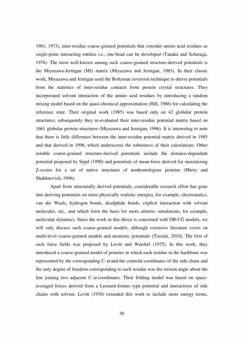
30

1961, 1973), inter-residue coarse-grained potentials that consider amino acid residues as

single-point interacting entities i.e., one-bead can be developed (Tanaka and Scheraga,

1976). The most well-known among such coarse-grained structure-derived potentials is

the Miyazawa-Jernigan (MJ) matrix (Miyazawa and Jernigan, 1985). In their classic

work, Miyazawa and Jernigan used the Boltzman inversion technique to derive potentials

from the statistics of inter-residue contacts from protein crystal structures. They

incorporated solvent interaction of the amino acid residues by introducing a random

mixing model based on the quasi-chemical approximation (Hill, 1986) for calculating the

reference state. Their original work (1985) was based only on 42 globular protein

structures; subsequently they re-evaluated their inter-residue potential matrix based on

1661 globular protein structures (Miyazawa and Jernigan, 1996). It is interesting to note

that there is little difference between the inter-residue potential matrix derived in 1985

and that derived in 1996, which underscores the robustness of their calculations. Other

notable coarse-grained structure-derived potentials include the distance-dependant

potential proposed by Sippl (1990) and potentials of mean-force derived for maximizing

Z-scores for a set of native structures of nonhomologous proteins (Mirny and

Shakhnovich, 1996).

Apart from structurally derived potentials, considerable research effort has gone

into deriving potentials on more physically realistic energies, for example, electrostatics,

van der Waals, hydrogen bonds, disulphide bonds, explicit interaction with solvent

molecules, etc., and which form the basis for more abinitio simulations, for example,

molecular dynamics. Since the work in this thesis is concerned with OB-CG models, we

will only discuss such coarse-grained models, although extensive literature exists on

multi-level coarse-grained models and atomistic potentials (Tozzini, 2010). The first of

such force fields was proposed by Levitt and Warshel (1975). In this work, they

introduced a coarse-grained model of proteins in which each residue in the backbone was

represented by the corresponding C-α and the centroid coordinates of the side chain and

the only degree of freedom corresponding to each residue was the torsion angle about the

line joining two adjacent C-α coordinates. Their folding model was based on space-

averaged forces derived from a Leonard-Jonnes type potential and interactions of side

chains with solvent. Levitt (1976) extended this work to include more energy terms,

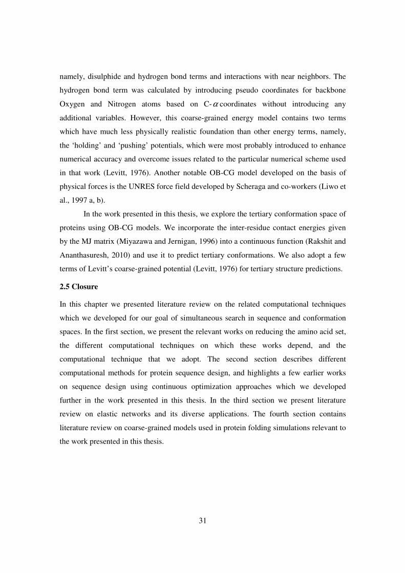
31

namely, disulphide and hydrogen bond terms and interactions with near neighbors. The

hydrogen bond term was calculated by introducing pseudo coordinates for backbone

Oxygen and Nitrogen atoms based on C-α coordinates without introducing any

additional variables. However, this coarse-grained energy model contains two terms

which have much less physically realistic foundation than other energy terms, namely,

the ‘holding’ and ‘pushing’ potentials, which were most probably introduced to enhance

numerical accuracy and overcome issues related to the particular numerical scheme used

in that work (Levitt, 1976). Another notable OB-CG model developed on the basis of

physical forces is the UNRES force field developed by Scheraga and co-workers (Liwo et

al., 1997 a, b).

In the work presented in this thesis, we explore the tertiary conformation space of

proteins using OB-CG models. We incorporate the inter-residue contact energies given

by the MJ matrix (Miyazawa and Jernigan, 1996) into a continuous function (Rakshit and

Ananthasuresh, 2010) and use it to predict tertiary conformations. We also adopt a few

terms of Levitt’s coarse-grained potential (Levitt, 1976) for tertiary structure predictions.

2.5 Closure

In this chapter we presented literature review on the related computational techniques

which we developed for our goal of simultaneous search in sequence and conformation

spaces. In the first section, we present the relevant works on reducing the amino acid set,

the different computational techniques on which these works depend, and the

computational technique that we adopt. The second section describes different

computational methods for protein sequence design, and highlights a few earlier works

on sequence design using continuous optimization approaches which we developed

further in the work presented in this thesis. In the third section we present literature

review on elastic networks and its diverse applications. The fourth section contains

literature review on coarse-grained models used in protein folding simulations relevant to

the work presented in this thesis.

32

3. Reduced Amino Acid Alphabet using Metric

Multi-dimensional Scaling (MMDS)

• We present the motivation behind reducing the amino acid set and using MMDS.

• The method of MMDS and the derivation of a low dimensional map from a set of

interconnected data are described.

• We use MMDS on the MJ matrix and present the results with suitable discussion.

• The chapter is closed by a brief summary.

3.1 Introduction

In this work we present a map based on the inter-residue contact energies given by the

Miyazawa-Jernigan (MJ) matrix (Miyazawa and Jernigan, 1996) using metric multi-

dimensional scaling (MMDS) (Kruskal, 1978). By presenting the data in a visual form,

we hope to reduce the complexity of finding out the inter-relations among the residues

which might not be directly evident from the MJ matrix. Each amino acid is represented

as a point on the MMDS map. The distance between two points on the map quantifies the

dissimilarity in their contact energies. The larger the distance the larger the dissimilarity.

This map elucidates relationships among the amino acids that are not easily discerned

from the MJ matrix.

The MMDS method is frequently used for a visual representation from a set of

data representing the relation among a number of objects. Similar work was reported by

French and Robson (1983) who had derived a map using MMDS for amino acids from

Dayhoff’s “relatedness odds matrix” (1972). The MMDS map presented in this chapter

verifies that hydrophobicity is the key feature that characterizes the amino acid residues

and the inter-residue contact energies represent a rough hydrophobicity scale (Cornette et

al., 1987, Chan, 1999, Venkatarajan and Braunn, 2001). Additionally, with the help of

this map, we compare (the similarities/differences among amino acid residues as

represented by) the MJ matrix with Block Substitution Matrix (BLOSUM) 62 (Heinkoff

and Heinkoff, 1992) and Pointwise Accepted Mutations (PAM) (Schwartz and Dayhoff,

1978) 250 matrices.

33

A novel feature of our map is that it can be used as a visual method of reducing

the amino acid set. We support this by determining the groups using a hierarchical

clustering method (Johnson and Wichern, 2006). We are also able to arrive at an

optimum number of groups for reducing the amino acid set by using this method.

3.2 Method

Metric Multi Dimensional Scaling (Mead, 1992) is a multi-variate statistical analysis

technique that is used for making a visual representation from a n n× matrix representing

the interaction between a set of n objects that one is interested to study. The thij entry in

the matrix represents the interaction between thi and thj objects. If the thij entry in the

matrix represents dissimilarity between the thi and thj objects, then the matrix is called

the dissimilarity or distance or proximity matrix. Here, as there can be no dissimilarity

between an object with itself all the diagonal elements are zero. On the other hand, if the

thij entry into the matrix represents similarity between the thi and thj objects, then the

matrix is called the similarity matrix. In this case, the diagonal elements are non-zero.

The results are represented as a plot of n points representing the n objects on a space of

two or higher dimensions. This method was first suggested by Torgerson (1952) and then

developed and used by Kruskal and Wish (1964) in representing as varied and qualitative

things as cultural similarity among nations and dialect of Salish Indians. More recently,

this map was used for classifying engineering materials based on ergonomic and aesthetic

considerations (Ashby and Johnson, 2002).

The key feature of MMDS method is that it reveals the hidden structure among

the objects that lies buried in the mass of data stored in a matrix form. Similar points are

huddled together in the plot and the distances among the points give a measure of

similarity among the objects. Furthermore, one can often identify variation of key

parameters on which these objects depend along different directions in the map.

Mathematically, constructing an MMDS map can be shown to be a least-square

minimization problem. Let n objects be represented by a set of n points on a plane. Let

the distance between thi and thj points be ij

d and its corresponding entry in the

34

proximity matrix is ij

δ . The MMDS technique attempts to minimize all such distances in

the sense of least squares, i.e. ,

( )( )2

2

,, 1

n

ij ij

i ji j

Minimize d δ=

≠

−∑x y

(3.1)

where,

1 2{ , , , }nx x x=x � and 1 2{ , , , }ny y y=y � are the x and y coordinates of the n points in

the map, and

( ) ( ) ( )2 22

ij i j i jd x x y y= − + − (3.2)

where the superscript in braces indicates the dimensionality of the MMDS map (in this

case it is two as we have chosen a planar representation). Therefore, we can write Eq. 3.1

as,

( ) ( )2

2 2

,, 1

n

i j i j ij

i ji j

Minimize x x y y δ=

≠

− + − −

∑

x y (3.3)

The solution of the minimization problem in Eq. 3.3 gives the coordinates of the points

and helps create the MMDS map. It should be noted that the MMDS map is unaffected

by the orientation of the chosen coordinate system, i.e., the final set of points may be

oriented differently in different runs with different initial guesses but the relative

positions of the points do not change. This happens because MMDS deals with only the

distances between the points which are devoid of any directional information. We have

used MATLAB’s optimization toolbox program fminunc (unconstrained optimization

which uses sequential quadratic programming combined with trust region method) to

solve the above least-square minimization problem in constructing the map. However, the

thij entry of the MJ matrix cannot be directly used as ijδ in Eq. 3.3. The treatment of the

MJ matrix to get the ijδ s is discussed next.

The thij entry in the MJ matrix represents the contact energy between thi and thj

amino acids. The diagonal entries represent contact energy between same amino acids.

Therefore, the extent to which the thij entry matches the corresponding diagonal entries

(both thi and thj diagonal entries) represents the similarity between the th

i and thj amino

35

acids. Thus, the MJ matrix can be taken as a similarity matrix. To convert the MJ matrix

to a proximity matrix we do the following operation:

2

ii jj

ij ij

M MMδ

+ = −

(3.4)

where , , and ii ii ijM M M are the , , and th th thii jj ij entries in the MJ matrix respectively.

Here, we take the absolute value as ijδ represents distance between two points and hence

is always positive. This symmetric transformation ensures that all the diagonal entries are

zero. With this matrix now one can select multiple dimensions (one and above) for

minimizing Eq. 3.3. For a given dimension it may not be possible to position all the

points on the map such that the distances among them exactly match the corresponding

distances given by the proximity matrix. The extent to which it deviates from the actual

data is given by a measure called stress (Kruskal and Wish, 1964). This stress is given

by,

( )( )2

2( )

q

ij ij

i j

i j

ij

i j

i j

d

Stress q

δ

δ<

<

−

=

∑∑

∑∑ (3.5)

where, q is the dimension of MMDS map. For example, when q is two ijd is given by

Eq. 3.2. The values of stress calculated for one, two and three dimensions are shown in

Fig. 3.1. We selected two as the dimension because stress is lowest there. We did not

Fig. 3.1. Plot of stress against number of dimensions

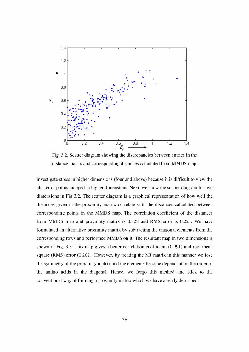
36

investigate stress in higher dimensions (four and above) because it is difficult to view the

cluster of points mapped in higher dimensions. Next, we show the scatter diagram for two

dimensions in Fig 3.2. The scatter diagram is a graphical representation of how well the

distances given in the proximity matrix correlate with the distances calculated between

corresponding points in the MMDS map. The correlation coefficient of the distances

from MMDS map and proximity matrix is 0.828 and RMS error is 0.224. We have

formulated an alternative proximity matrix by subtracting the diagonal elements from the

corresponding rows and performed MMDS on it. The resultant map in two dimensions is

shown in Fig. 3.3. This map gives a better correlation coefficient (0.991) and root mean

square (RMS) error (0.202). However, by treating the MJ matrix in this manner we lose

the symmetry of the proximity matrix and the elements become dependant on the order of

the amino acids in the diagonal. Hence, we forgo this method and stick to the

conventional way of forming a proximity matrix which we have already described.

ijd

ijδ

Fig. 3.2. Scatter diagram showing the discrepancies between entries in the

distance matrix and corresponding distances calculated from MMDS map.

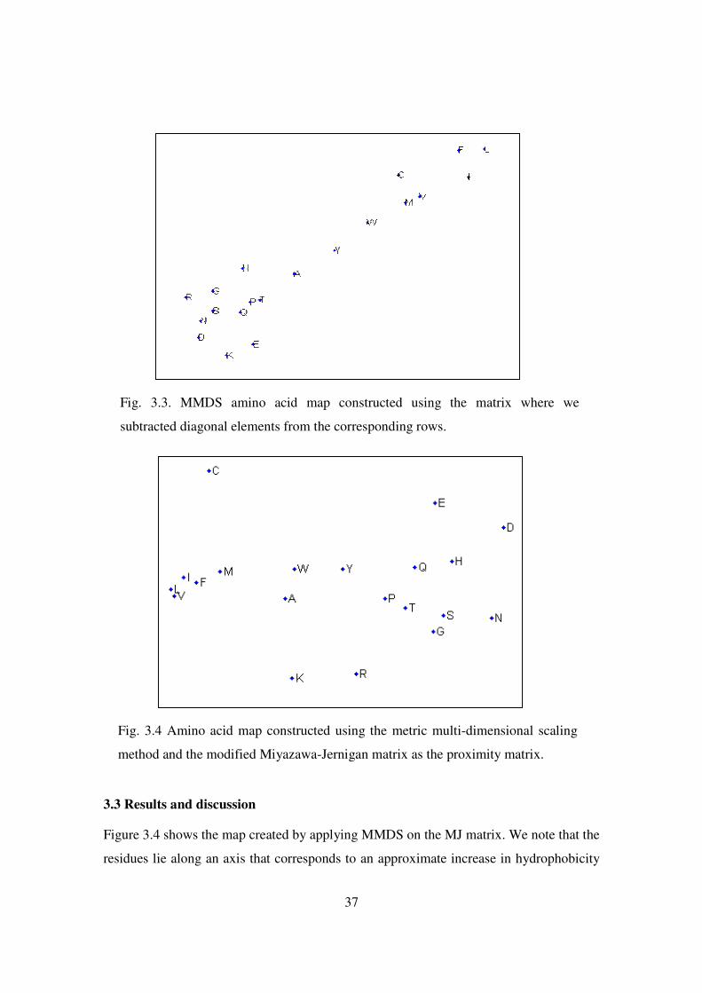
37

3.3 Results and discussion

Figure 3.4 shows the map created by applying MMDS on the MJ matrix. We note that the

residues lie along an axis that corresponds to an approximate increase in hydrophobicity

Fig. 3.4 Amino acid map constructed using the metric multi-dimensional scaling

method and the modified Miyazawa-Jernigan matrix as the proximity matrix.

Fig. 3.3. MMDS amino acid map constructed using the matrix where we

subtracted diagonal elements from the corresponding rows.

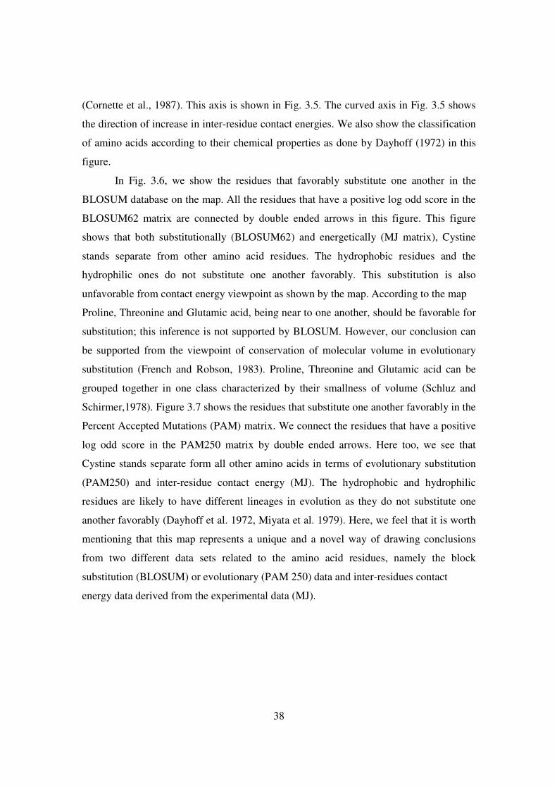
38

(Cornette et al., 1987). This axis is shown in Fig. 3.5. The curved axis in Fig. 3.5 shows

the direction of increase in inter-residue contact energies. We also show the classification

of amino acids according to their chemical properties as done by Dayhoff (1972) in this

figure.

In Fig. 3.6, we show the residues that favorably substitute one another in the

BLOSUM database on the map. All the residues that have a positive log odd score in the

BLOSUM62 matrix are connected by double ended arrows in this figure. This figure

shows that both substitutionally (BLOSUM62) and energetically (MJ matrix), Cystine

stands separate from other amino acid residues. The hydrophobic residues and the

hydrophilic ones do not substitute one another favorably. This substitution is also

unfavorable from contact energy viewpoint as shown by the map. According to the map

Proline, Threonine and Glutamic acid, being near to one another, should be favorable for

substitution; this inference is not supported by BLOSUM. However, our conclusion can

be supported from the viewpoint of conservation of molecular volume in evolutionary

substitution (French and Robson, 1983). Proline, Threonine and Glutamic acid can be

grouped together in one class characterized by their smallness of volume (Schluz and

Schirmer,1978). Figure 3.7 shows the residues that substitute one another favorably in the

Percent Accepted Mutations (PAM) matrix. We connect the residues that have a positive

log odd score in the PAM250 matrix by double ended arrows. Here too, we see that

Cystine stands separate form all other amino acids in terms of evolutionary substitution

(PAM250) and inter-residue contact energy (MJ). The hydrophobic and hydrophilic

residues are likely to have different lineages in evolution as they do not substitute one

another favorably (Dayhoff et al. 1972, Miyata et al. 1979). Here, we feel that it is worth

mentioning that this map represents a unique and a novel way of drawing conclusions

from two different data sets related to the amino acid residues, namely the block

substitution (BLOSUM) or evolutionary (PAM 250) data and inter-residues contact

energy data derived from the experimental data (MJ).

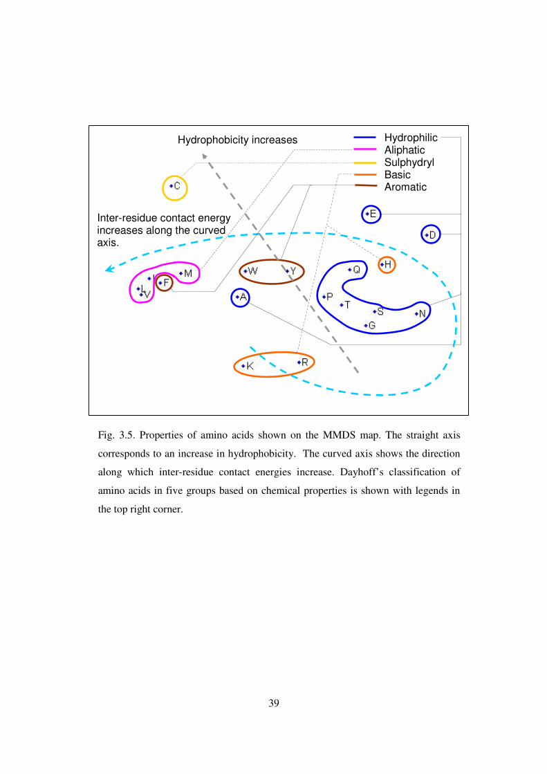
39

Fig. 3.5. Properties of amino acids shown on the MMDS map. The straight axis

corresponds to an increase in hydrophobicity. The curved axis shows the direction

along which inter-residue contact energies increase. Dayhoff’s classification of

amino acids in five groups based on chemical properties is shown with legends in

the top right corner.

Inter-residue contact energy increases along the curved axis.

Hydrophobicity increases Hydrophilic Aliphatic Sulphydryl Basic Aromatic

40

Fig. 3.7. The residues that have a positive log odd score in the PAM250

matrix are connected by double ended arrows.

Fig. 3.6. The residues that have a positive log odd score in the BLOSUM62

matrix are connected by double ended arrows.

41

Reducing the amino acid residues to a small set is a topic of active interest among protein

researchers. A few works based on the MJ matrix exist in the current literature (Wang

and Wang, 2002 and 1999, Cieplak et al., 2001, Li et al., 1997). All these works employ

different methods for reducing the amino acid set. The MMDS method provides an easy

visual method of grouping (see Fig. 3.4). To reinforce this, we use a hierarchical

clustering method based on average distance of clusters (Johnson and Wichern, 2006) on

our distance matrix to simplify the amino acid set. In this method, we find the minimum

distance in the distance matrix and group the corresponding amino acids. Next, we find

the distance between this group and all other amino acids by calculating the mean

distance from this group to all other amino acids or groups. Thus, if L (Leucine) and I

(Isoleucine) are clubbed together to form a group {L,I}, then the distance { },L I Gd of this

group from G (Glycine) is given by 2

LG IGd d+

. We continue this procedure starting

from 20 amino acids and go on grouping until we arrive at a single group. The resulting

dendrogram is shown in Fig. 3.8.

In Fig. 3.9 we plot the minimum distance between the groups as we go on

decreasing the number of groups. We see that the highest ratio of increase in the

minimum distance to the current minimum distance occurs when the number of clusters

changes from 19 to 18 and from five to four or four to three. A sudden increase in

minimum distance indicates that the groups are losing their compact size as they are

merged together. Since 18 is a large number for reducing the amino acid set we conclude

that five or four is the best number for simplifying the amino acid set. Our conclusion is

further supported by the fact that grouping amino acid residues into five sets is most

common in the literature (Dayhoff et al., 1972, Li et al., 1997, Wolynes, 1997, Murphy et

al., 2000, Wang and Wang, 2002 and 1999, Cieplak et al., 2001, Cannata et al., 2002, Li

et al., 2003, Koisol et al., 2004). In Fig. 3.10 we show these five groupings on our

MMDS map. Although our grouping is based on hierarchical clustering and our database

is contact energies from a statistical database we find distinctive chemical properties

within each group. D and E are acidic whereas K and R have basic properties. Q, H, P, T,

42

Fig. 3.8. Dendrogram showing hierarchical grouping of amino acids based on our distance matrix.

CMFILVWYAGTSNQDEHRKP

C MFILVWYAGTSNQDEHRKP

C MFILVWYAKR GTSNQDEHP

C MFILVWYA KR GTSNQDEHP

C MFILVWYA KR GTSNQHP DE

C KR WYA MFILV DE GTSNQHP

C KR WYA MFILV DE QH GTSNP

C KR WYA MFILV D QH GTSNP E

C KR D QH TP WYA MFILV E GSN

C KR D QH TP WY MFILV E GSN A

C K D QH TP WY MFILV E GSN A R

C K D QH TP

W

E GS

Y

R A MFILV WY N

C K D QH TP E GS R A MFILV

N

W Y C K D QH TP E GS R A FILV

N M

W Y C K D Q TP E GS R A FILV

N M H

W Y C K D Q TP E G R A FILV

N M H S

W Y C K D Q TP E G R A FI

N M H S LV

W Y C K D Q T E R A FI N

M H S LV P G

W Y C K D Q T E R A F N

M H S LV P G I

W Y C K D Q T E R A F N

M H S L P G I V

43

S, G, N all have small molecular volume and are hydrophilic in nature. On the other

hand L, V, I, M, F, W, Y (all except A in that group) are characterized by their largeness

in size and hydrophobic nature. Lastly, C stands alone because of its unique ability to

form disulphide bonds.

Fig. 3.9. Minimum distance between groups as a function of the number of groups.

The ratio of increase in minimum distance (between groups) as we reduce the

number of groups to the minimum distance (between groups) in current number of

groups is highest for 18 and five groups.

44

3.4 Closure

In this chapter we presented a map of the amino acids using the metric-multidimensional

scaling method. By applying this method on the MJ matrix we were able to uncover the

underlying similarities among the amino acids in the map. The map also enabled us to

compare the MJ matrix with other scoring matrices like the PAM and BLOSUM. Finally

we presented a hierarchic grouping scheme for the amino acids from which the best

number of reduced amino acid alphabets was deduced.

Fig. 3.10. Grouping of amino acids into five groups based on hierarchical clustering

method. This grouping coincides if one goes for clustering amino acids into five

groups on MDS map based on visual inspection alone. The hierarchical clustering in

Fig. 3.8 can also be done from our MDS map by mere visual inspection.

45

4. Search in the Sequence Space

• We give an introduction to protein sequence design for fixed backbone and its

relevance in simultaneous sequence and conformation search.

• We describe sequence design using double sigmoid interpolation technique and

apply it to design sequences for four proteins.

• We present sequence design using quadratic programming and test it on four

proteins.

• We compare the two methods and find out the relative advantages and drawbacks.

• We close the section by a brief summary.

4.1 Introduction

The sequence design problem, also known as “the inverse folding problem” (Drexler,

1981) has gained as much importance as the “protein folding problem” with recent

successes in the development of de-novo proteins (Hecht et al., 1990, Desjarlais and

Handel, 1995, Dahiyat and Mayo, 1996, 1997, Dahiyat et al., 1997, Street and Mayo,

1999, Dantas et al., 2003, Kuhlman et al., 2003, Offredi et al., 2003, Butterfoss and

Kuhlman, 2006). De-novo proteins with new folds (Farinas and Regan, 2003), higher

stability (Gillespie et al., 2003) and faster folding rates (Kuhlman et al., 2002, Dantas et

al., 2003) are giving new insights into the intricate mechanism by which proteins fold in-

vivo. A key to the success of designing a de-novo protein lies in the accurate specification

of sequences that will fold to a given target structure. With the help of computational

tools geared towards searching the vast sequence space efficiently, experimentalists can

save much effort and cost.

As discussed in the literature review section, to the best of our knowledge, all

computational sequence design techniques use discrete or heuristic optimization methods

for searching the sequence space. As mentioned earlier, our work is motivated by the

recent works of a few researchers (Koh et al. 2005, Koh et al. 2005, Ananthasuresh 2006,

Jha et al. 2006, Koh et al. 2009, Jha et al. 2009) in formulating protein sequence design

as a continuous optimization problem. In this work, we propose a novel continuous

formulation for protein sequence design using the double sigmoid function using

46

different potential functions (statistical and atomistic) and also extend the quadratic

programming formulation for protein sequence design (Koh et al., 2005) to all 20 amino

acids using atomistic potentials.

We demonstrate our methods on a set of four proteins, namely, homeodomain

chain C, PDB (Bernstein et al., 1977) ID 1HDD (Kissinger et al., 1990); calbindin, PDB

ID 4ICB (Svensson et al., 1992); protein A of human Fc fragment chain C, PDB ID 1FC2

(Deisenhofer, 1981) and Cro repressor, PDB ID 2CRO (Mondragon, et al. 1989b). The

native structures of these proteins are shown in Fig. 4.1. Our selection is based on the

FISA decoy set (Simons et al., 1997), which contains 500 decoy structures for each of the

2CRO 65 residues

1FC2 (chain C) 43 residues

1HDD (chain C) 57 residues

4ICB 76 residues

Fig. 4.1. Native structure of the four proteins that we target for sequence design.

The number of residues in each protein is also indicated.

47

aforementioned four proteins. We have used gradient-based large-scale nonlinear

optimization problem solver IPOPT (Wächter, 2002, Wächter and Biegler, 2004) (Please

refer to Appendix B1 for a short discussion on IPOPT) to design minimum energy

sequences for the abovementioned proteins. We align the designed sequences with the

wild-type sequences and find the site-specific amino acid residue matches without

inserting any gaps. The criterion for finding matches without inserting gaps is a stringent

criterion. Many sequence alignment programs align sequences by inserting gaps within

them. We, however, follow a different path by aligning sequences without gaps and

develop a novel scoring method by not only counting site-specific matches but also the

same based on simplified amino acid alphabet (Dayhoff et al., 1978, Wang and Wang,

1999, 2002, Murphy et al., 2000, Cieplak et al., 2001, Cannata et al., 2002, Li et al.,

2003, Koisol et al., 2004, Rakshit and Ananthasuresh, 2008). Reduced amino acid

alignment has been used for checking the designability of sequences (Brown et al., 2003).

Our results are satisfactory both for non-reduced and reduced amino acid set. When we

align our design sequences with the wild-type ones by using the CLUSTAL (version

1.83) (Higgins and Sharp, 1988), a software that inserts gaps for maximum alignment, we

find the number of matches increase, as expected. We also test our designed sequences by

threading them on the decoy set FISA for the aforementioned proteins (Simons et al.,

1997).

Before proceeding to the description of our sequence design methods, we would

like to specifically mention the scope of our sequence design formulations. Both the

formulations described here are based on the principle of minimization of free energy,

which governs protein folding (Anfinsen, 1961, 1973). Although wild-type sequences are

the outcomes of a complex interplay of various selective pressures, minimization of free

energy plays an important role in selecting them (Dill and Chan, 1997). Furthermore,

Shakhnovich and Gutin (1993) used lattice models to demonstrate that the minimum

energy sequences are also the ones that fold at faster rate than random sequences.

However, free energy minimization is not the best method for designing de novo protein

sequences, especially based on statistical potentials (Yue et al., 1995, Thomas and Dill,

1996, Moult, 1997, Zhang and Skolnick, 1998). Based on structural information of the

native-state, formulations have been developed to design sequences to maximize the Z-

48

score, i.e., maximization of the energy gap between native and competing structures and

minimization of the fluctuation of energy over all native-like structures (Deutsch and

Kurosky, 1996, Morrissey and Shakhnovich, 1996, Seno et al., 1996, Mirny and

Shakhnovich, 1996). Z-score optimization has also been used to calculate statistical

potentials or statistically tuned physical potentials specifically for guiding designed

sequences to fold to target structures (Koehl and Delarue, 1996, Dahiyat and Mayo, 1997,

Chiu and Goldstein, 1998, Zhang and Skolnick, 1998, Gordon and Mayo, 1999, Mendes

et al., 2002, Dokholyan, 2004, Gordon et al., 1999, Liang and Grishin, 2004, Pokala and

Handel, 2005, Alvizo and Mayo, 2008). However, in this work, we do simultaneous

search in sequence and conformation spaces. Z-score based potentials or Z-score based

formulations are not amenable to use when both sequence and conformation are

unknown. For this reason, we base our formulations on minimization of free energy

rather than Z-score.

In the first phase of simultaneous sequence and conformation search, when both

are unknown, we use statistical potentials to design sequences (our simultaneous

sequence and conformation search strategy will be described in detail in Chapter 6). The

applicability of statistical potentials has been argued for de novo sequence design (Yue et

al., 1995, Thomas and Dill 1996, Moult 1997, Zhang and Skolnick 1998). Hence, in the

subsequent sections where we evaluate our sequence design formulations, we present the

best designed sequences not on the basis of the energy of the designed sequences, but by

matching them against the wild-type sequences and also by calculating the energy gap

and dispersion of energy of the designed sequences. Thus, the above two criteria, i.e., the

number of matches with wild-type sequences and the calculation of the energy gap and

dispersion of energies based on decoy sets, serve as alternative tests for our formulation

of sequence design based on continuous optimization.

The rest of this chapter is organized as follows. We next describe our sequence

design formulations using the double sigmoid function. Thereafter, we present the results

using this method. In the following section, we describe sequence design formulation

using quadratic programming. After that, we present the results using quadratic

programming approach on the same set of proteins. We end the chapter with a discussion

of both the methods.

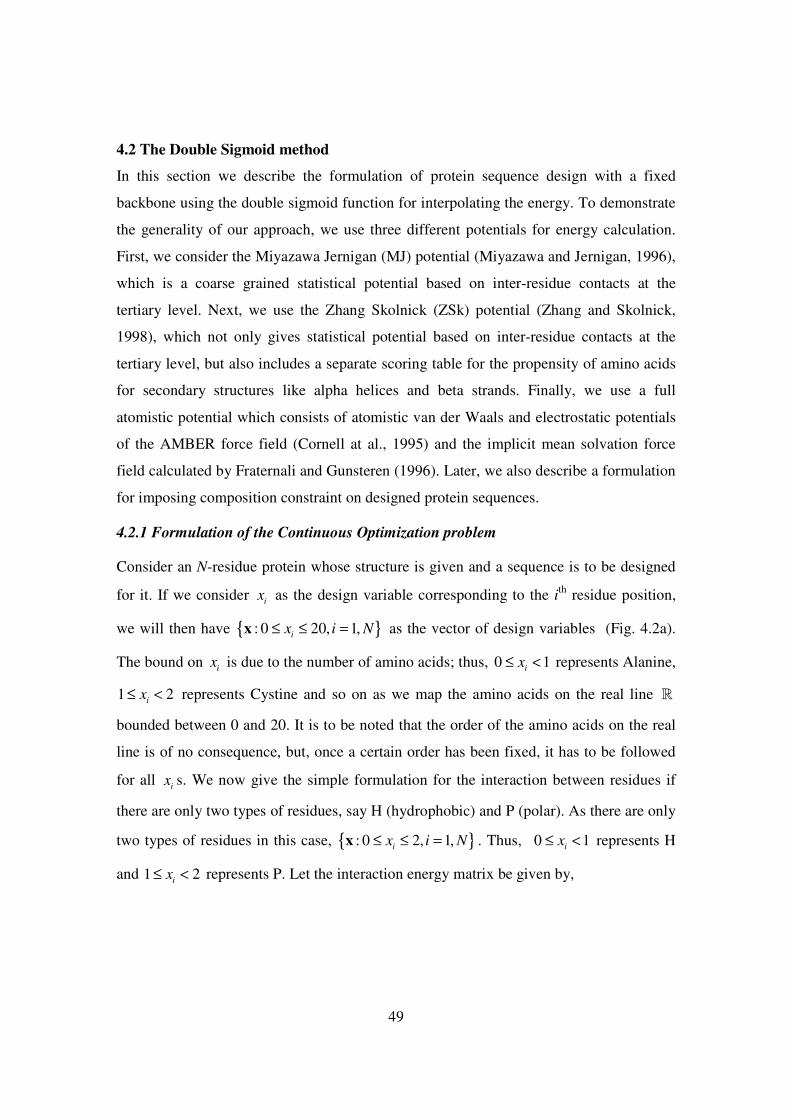
49

4.2 The Double Sigmoid method

In this section we describe the formulation of protein sequence design with a fixed

backbone using the double sigmoid function for interpolating the energy. To demonstrate

the generality of our approach, we use three different potentials for energy calculation.

First, we consider the Miyazawa Jernigan (MJ) potential (Miyazawa and Jernigan, 1996),

which is a coarse grained statistical potential based on inter-residue contacts at the

tertiary level. Next, we use the Zhang Skolnick (ZSk) potential (Zhang and Skolnick,

1998), which not only gives statistical potential based on inter-residue contacts at the

tertiary level, but also includes a separate scoring table for the propensity of amino acids

for secondary structures like alpha helices and beta strands. Finally, we use a full

atomistic potential which consists of atomistic van der Waals and electrostatic potentials

of the AMBER force field (Cornell at al., 1995) and the implicit mean solvation force

field calculated by Fraternali and Gunsteren (1996). Later, we also describe a formulation

for imposing composition constraint on designed protein sequences.

4.2.1 Formulation of the Continuous Optimization problem

Consider an N-residue protein whose structure is given and a sequence is to be designed

for it. If we consider ix as the design variable corresponding to the ith residue position,

we will then have { }: 0 20, 1,ix i N≤ ≤ =x as the vector of design variables (Fig. 4.2a).

The bound on ix is due to the number of amino acids; thus, 0 1ix≤ < represents Alanine,

1 2ix≤ < represents Cystine and so on as we map the amino acids on the real line �

bounded between 0 and 20. It is to be noted that the order of the amino acids on the real

line is of no consequence, but, once a certain order has been fixed, it has to be followed

for all ix s. We now give the simple formulation for the interaction between residues if

there are only two types of residues, say H (hydrophobic) and P (polar). As there are only

two types of residues in this case, { }: 0 2, 1,ix i N≤ ≤ =x . Thus, 0 1ix≤ < represents H

and 1 2ix≤ < represents P. Let the interaction energy matrix be given by,

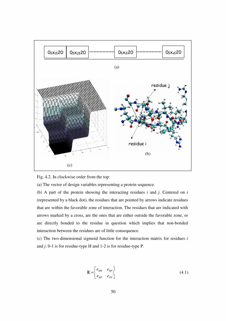
50

HH HP

HP PP

e e

e e

=

E (4.1)

Fig. 4.2. In clockwise order from the top:

(a) The vector of design variables representing a protein sequence.

(b) A part of the protein showing the interacting residues i and j. Centered on i

(represented by a black dot), the residues that are pointed by arrows indicate residues

that are within the favorable zone of interaction. The residues that are indicated with

arrows marked by a cross, are the ones that are either outside the favorable zone, or

are directly bonded to the residue in question which implies that non-bonded

interaction between the residues are of little consequence.

(c) The two-dimensional sigmoid function for the interaction matrix for residues i

and j. 0-1 is for residue-type H and 1-2 is for residue-type P.

0≤x1≤20 0≤x2≤20 0≤xi≤20 0≤xn≤20

(a)

residue i

residue j

(b)

(c)

51

When residues i and j are within the interaction distance as shown in Fig. 4.2b (the

interaction distance is taken as 6.5 Å from the C-α coordinates), the contact energy

between the residues is given by each element of E for each type of residue in Eq. 4.1,

i.e., when residue i is H ( 0 1ix≤ < ) and residue j is H ( 0 1j

x≤ < ), energy of interaction

is HHe , when residue i is H ( 0 1ix≤ < ) and residue j is P (1 2jx≤ < ), energy of

interaction is HPe , and so on. A continuous function representation of the matrix in

Eq. 4.1 is shown in Fig. 4.2c and the mathematical formula is a two-dimensional sigmoid

function as shown below,

( )

( )( )( )

( )( )( )

( )( ) ( )( )

1 1

2

1 1

j jii

j jii

HP HHHHij x xc xx

HP HH PP HP HH

c x c xc xx

e eeE

e e e e

e e e e e

e e e e

α ααα

α ααα

− −−−

− −−−

−= + +

+ + + +

− − ++

+ + + +

(4.2)

where,

α = smoothening parameter of the sigmoid function

= 25

c = 1

In a similar manner, the two-dimensional sigmoid function for twenty amino acids can be

constructed. Thus, for 20 amino acids, the formula is given by,

( ) ( )( )20 20

111 1

( , )

1 ji

ijx jx i

j i

f i jE

e eαα − − +− − +

= =

=+ +

∑∑ (4.3)

where the function ( , )f i j is given by,

( , ) ( , ) ( , )f i j M i j g i j= + (4.4)

where,

( , )M i j = the ijth value of the inter-residue contact energy matrix

and ( , )g i j is obtained recursively as,

( )( ) ( )1 1

(1,1) (1,1)

( , )( , ) ( , ) 1, 1

1

ji

i k j mk m

g M

g k mg i j M i j i j

e eβ ε β ε− + − − + −

= =

=

= − > >+ +

∑∑ (4.5)

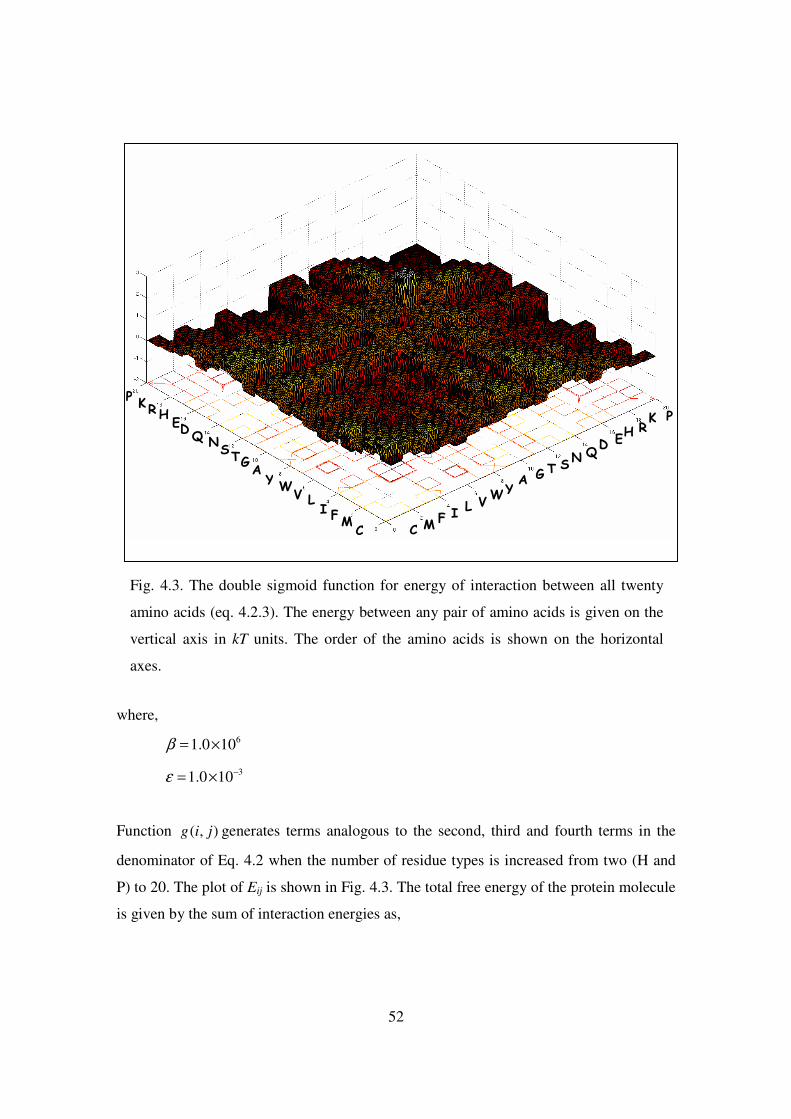
52

where,

61.0 10β = ×

31.0 10ε −= ×

Function ( , )g i j generates terms analogous to the second, third and fourth terms in the

denominator of Eq. 4.2 when the number of residue types is increased from two (H and

P) to 20. The plot of Eij is shown in Fig. 4.3. The total free energy of the protein molecule

is given by the sum of interaction energies as,

Fig. 4.3. The double sigmoid function for energy of interaction between all twenty

amino acids (eq. 4.2.3). The energy between any pair of amino acids is given on the

vertical axis in kT units. The order of the amino acids is shown on the horizontal

axes.

P

C M F I

L W Y A G T S

N Q

D E H R K

C M F I L

W Y A G T S

N Q

D E H R K

V V

P P

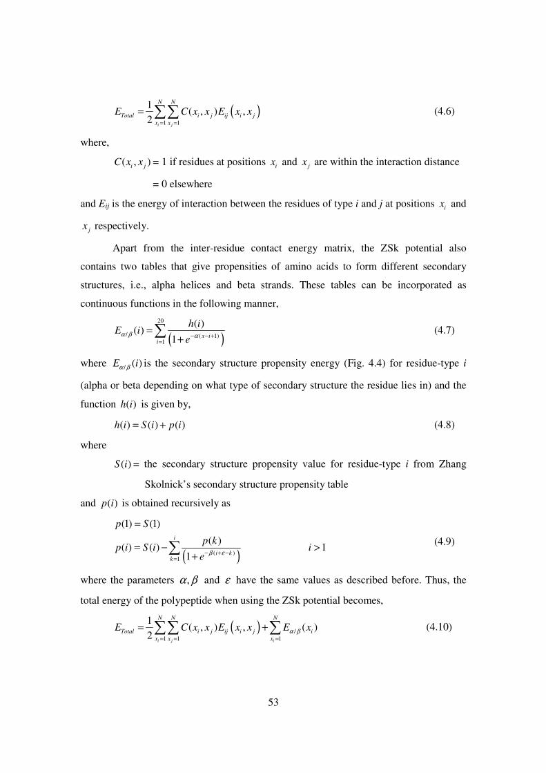
53

( )1 1

1( , ) ,

2i j

N N

Total i j ij i j

x x

E C x x E x x= =

= ∑∑ (4.6)

where,

( , )i jC x x = 1 if residues at positions ix and jx are within the interaction distance

= 0 elsewhere

and Eij is the energy of interaction between the residues of type i and j at positions ix and

jx respectively.

Apart from the inter-residue contact energy matrix, the ZSk potential also

contains two tables that give propensities of amino acids to form different secondary

structures, i.e., alpha helices and beta strands. These tables can be incorporated as

continuous functions in the following manner,

( )

20

/ ( 1)1

( )( )

1 x ii

h iE i

eα β α− − +

=

=+

∑ (4.7)

where / ( )E iα β is the secondary structure propensity energy (Fig. 4.4) for residue-type i

(alpha or beta depending on what type of secondary structure the residue lies in) and the

function ( )h i is given by,

( ) ( ) ( )h i S i p i= + (4.8)

where

( )S i = the secondary structure propensity value for residue-type i from Zhang

Skolnick’s secondary structure propensity table

and ( )p i is obtained recursively as

( )( )1

(1) (1)

( )( ) ( ) 1

1

i

i kk

p S

p kp i S i i

eβ ε− + −

=

=

= − >+

∑ (4.9)

where the parameters ,α β and ε have the same values as described before. Thus, the

total energy of the polypeptide when using the ZSk potential becomes,

( ) /1 1 1

1( , ) , ( )

2i j i

N N N

Total i j ij i j i

x x x

E C x x E x x E xα β= = =

= +∑∑ ∑ (4.10)

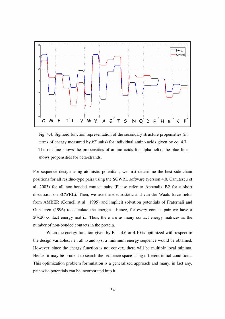
54

For sequence design using atomistic potentials, we first determine the best side-chain

positions for all residue-type pairs using the SCWRL software (version 4.0, Canutescu et

al. 2003) for all non-bonded contact pairs (Please refer to Appendix B2 for a short

discussion on SCWRL). Then, we use the electrostatic and van der Waals force fields

from AMBER (Cornell at al., 1995) and implicit solvation potentials of Fraternali and

Gunsteren (1996) to calculate the energies. Hence, for every contact pair we have a

20×20 contact energy matrix. Thus, there are as many contact energy matrices as the

number of non-bonded contacts in the protein.

When the energy function given by Eqs. 4.6 or 4.10 is optimized with respect to

the design variables, i.e., all xi and xj s, a minimum energy sequence would be obtained.

However, since the energy function is not convex, there will be multiple local minima.

Hence, it may be prudent to search the sequence space using different initial conditions.

This optimization problem formulation is a generalized approach and many, in fact any,

pair-wise potentials can be incorporated into it.

Fig. 4.4. Sigmoid function representation of the secondary structure propensities (in

terms of energy measured by kT units) for individual amino acids given by eq. 4.7.

The red line shows the propensities of amino acids for alpha-helix; the blue line

shows propensities for beta-strands.

C M F I L V W Y A G T S N Q D E H R K P

55

4.2.2 Formulation of the constraints

In cases when the amino acid composition of the target sequences are known, one may be

interested in designing sequences keeping the amino acid composition fixed. As proposed

by Koehl and Levitt (1999, 2002), this criterion ensures that the designed sequences are

specific to the target structure. In our optimization problem formulation, we can

incorporate the amino acid composition constraints. Let there be km numbers of residue

type k for each of the twenty types of amino acids. Then,

20

1k

k

m N=

=∑ (4.11)

where N is the total number of residues in the protein. km is related to the design

variables by the equation,

( )( ) ( )( )1 2

1

1 1

1 1i i

N

kx c x ci

me e

α α− −=

− =

+ + ∑ (4.12)

where 1c and 2c are the upper and lower ranges for residue type k, i.e., for example,

1c = 0.0 and 2c = 1.0 for Cystine from Fig. 4.3 and α is the smoothness parameter for the

sigmoid function. The plot of constraints against each residue position is shown in Fig.

4.5.

We would like to mention here that due to incorporation of such nonlinear

constraints (one constraint for each type of residue), often, optimization doesn’t

converge.

4.2.3 Results

As mentioned before, we choose a set of four proteins (PDB IDs 1FC2 chain C, 1HDD

chain C, 2CRO and 4ICB) to test our method. Even though we design sequences solely

based on minimization of the energy as given by Eq. 4.6 or 4.10, we thread the designed

sequences on the decoy set structures and check for specificity by calculating the energy

gap between the native structure and other structures in the decoy set and also standard

deviation of sequence energies over the structures in the same decoy set. Based on the

design criteria, i.e., minimization of energy and different initial values of the design

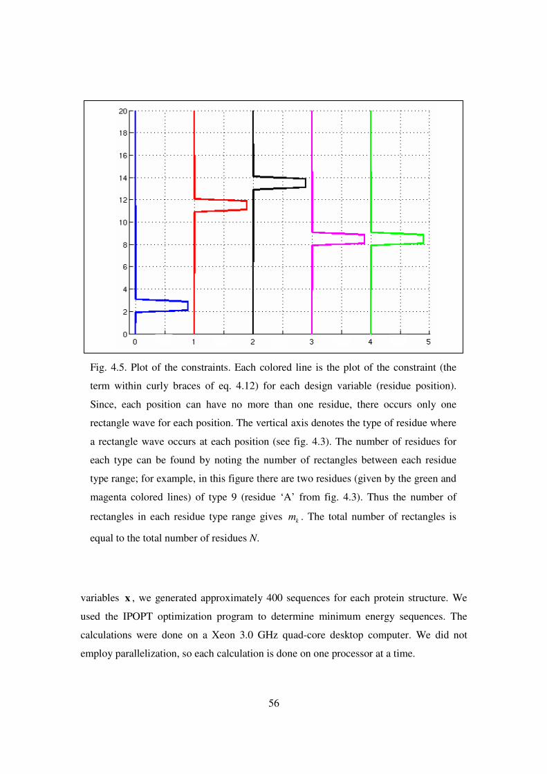
56

variables x , we generated approximately 400 sequences for each protein structure. We

used the IPOPT optimization program to determine minimum energy sequences. The

calculations were done on a Xeon 3.0 GHz quad-core desktop computer. We did not

employ parallelization, so each calculation is done on one processor at a time.

Fig. 4.5. Plot of the constraints. Each colored line is the plot of the constraint (the

term within curly braces of eq. 4.12) for each design variable (residue position).

Since, each position can have no more than one residue, there occurs only one

rectangle wave for each position. The vertical axis denotes the type of residue where

a rectangle wave occurs at each position (see fig. 4.3). The number of residues for

each type can be found by noting the number of rectangles between each residue

type range; for example, in this figure there are two residues (given by the green and

magenta colored lines) of type 9 (residue ‘A’ from fig. 4.3). Thus the number of

rectangles in each residue type range gives km . The total number of rectangles is

equal to the total number of residues N.

57

To demonstrate the generality of our approach, we use three different potentials for

energy calculation. As mentioned before, these are the Miyazawa Jernigan (MJ), Zhang

Skolnick (ZSk), and the atomistic potentials based on electrostatic and van der Waal’s

parameter values from the AMBER force field and solvation energy from implicit

solvation model of Fraternali and Gunsteren. For each protein, we design sequences both

with and without amino acid composition constraints. After designing the sequences we

align them with the corresponding wild-type sequence of each protein. For finding the

best sequence based on alignment, we not only calculate the number of amino acid

matches but also the matches based on the reduced amino acid sets. Apart from

hydrophobic-hydrophilic grouping of amino acids, we find grouping amino acids into

five sets most common in the literature. Here, we select 10 different five-letter grouping

schemes (Dayhoff et al. 1978, Wang and Wang 1999, Murphy et al. 2000, Cieplak et al.

2001, Cannata et al. 2002, Wang and Wang 2002, Li et al. 2003, Koisol et al. 2004,

Rakshit and Ananthasuresh 2008) based on different criteria and calculate matches

between designed and wild-type sequences after aligning them. Each grouping scheme

uses its own method for reducing the amino acid set and brings out common

characteristics between different amino acids based on which they are grouped. For

example, whereas Dayhoff’s classification (1978) is based on evolutionary criteria and

calculated using the PAM matrix, Rakshit and Ananthasuresh’s classification (2008) is

based on hydrophobicity-hydrophilicity criterion and calculated using the MJ matrix. We

calculate the total number of reduced-alphabet matches for each designed sequence based

on all grouping methods and add the number of non-reduced matches after weighting

them by a factor of four. This factor is introduced to compensate for the loss of

specificity from twenty to five letters. We can thus rank the designed sequences based on

a score given by

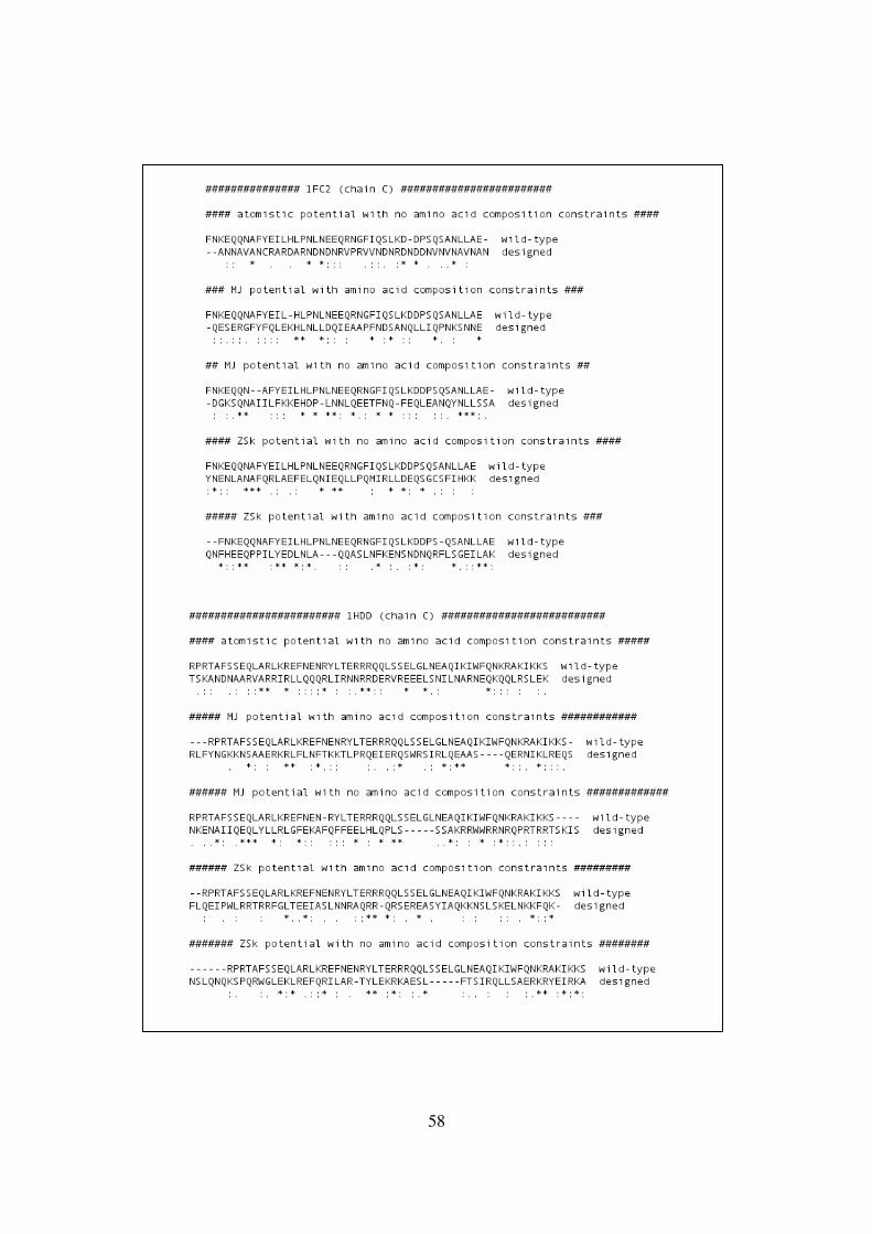
58

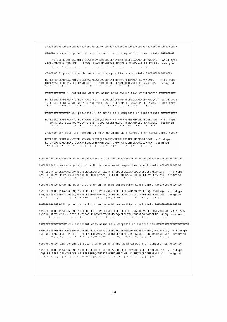
59

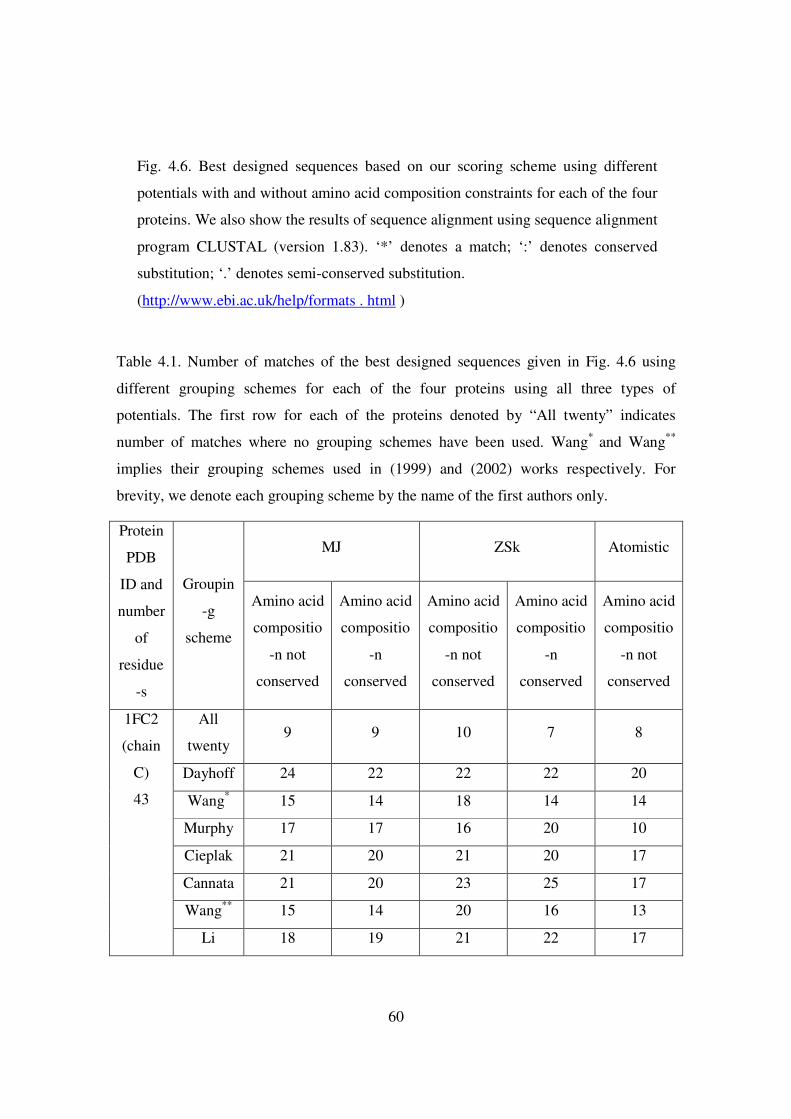
60

Table 4.1. Number of matches of the best designed sequences given in Fig. 4.6 using

different grouping schemes for each of the four proteins using all three types of

potentials. The first row for each of the proteins denoted by “All twenty” indicates

number of matches where no grouping schemes have been used. Wang* and Wang**

implies their grouping schemes used in (1999) and (2002) works respectively. For

brevity, we denote each grouping scheme by the name of the first authors only.

MJ ZSk Atomistic Protein

PDB

ID and

number

of

residue

-s

Groupin

-g

scheme

Amino acid

compositio

-n not

conserved

Amino acid

compositio

-n

conserved

Amino acid

compositio

-n not

conserved

Amino acid

compositio

-n

conserved

Amino acid

compositio

-n not

conserved

All

twenty 9 9 10 7 8

Dayhoff 24 22 22 22 20

Wang* 15 14 18 14 14

Murphy 17 17 16 20 10

Cieplak 21 20 21 20 17

Cannata 21 20 23 25 17

Wang** 15 14 20 16 13

1FC2

(chain

C)

43

Li 18 19 21 22 17

Fig. 4.6. Best designed sequences based on our scoring scheme using different

potentials with and without amino acid composition constraints for each of the four

proteins. We also show the results of sequence alignment using sequence alignment

program CLUSTAL (version 1.83). ‘*’ denotes a match; ‘:’ denotes conserved

substitution; ‘.’ denotes semi-conserved substitution.

(http://www.ebi.ac.uk/help/formats . html )

61

Koisol 27 27 28 27 25

Rakshit 18 15 20 16 16

All

twenty 12 9 10 8 9

Dayhoff 23 17 26 17 28

Wang* 20 19 23 20 27

Murphy 16 13 21 10 23

Cieplak 26 24 27 24 28

Cannata 26 20 30 23 31

Wang** 20 17 21 17 22

Li 23 20 28 19 29

Koisol 34 32 37 32 39

1 HDD

(chain

C)

57

Rakshit 21 15 23 14 22

All

twenty 11 11 10 14 10

Dayhoff 26 28 29 29 24

Wang* 24 19 29 25 22

Murphy 18 21 24 22 18

Cieplak 26 22 24 26 21

Cannata 26 27 33 23 25

Wang** 20 16 21 22 20

Li 23 24 29 20 23

Koisol 35 35 38 38 33

2 CRO

65

Rakshit 26 24 28 30 23

All

twenty 16 14 14 13 12

Dayhoff 36 34 37 34 33

Wang* 32 24 26 21 25

Murphy 25 24 26 24 22

4 ICB

76

Cieplak 38 34 38 29 30

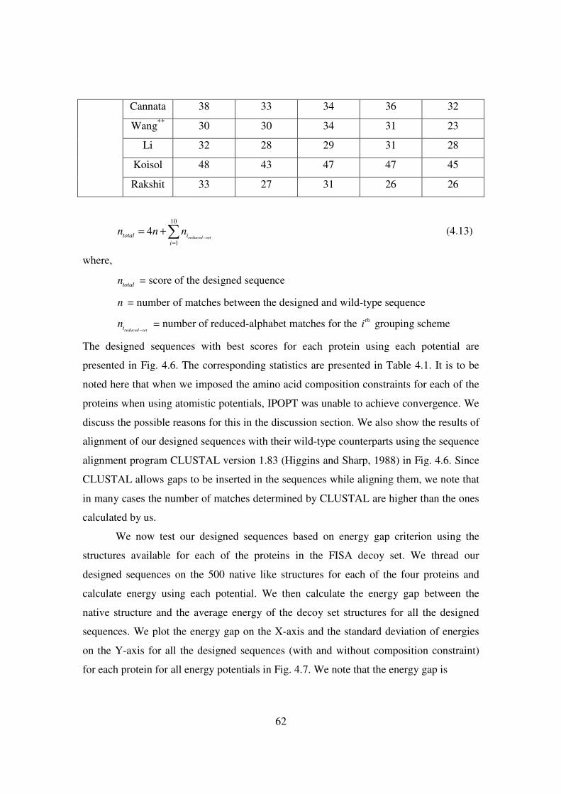
62

Cannata 38 33 34 36 32

Wang** 30 30 34 31 23

Li 32 28 29 31 28

Koisol 48 43 47 47 45

Rakshit 33 27 31 26 26

10

1

4reduced settotal i

i

n n n−

=

= +∑ (4.13)

where,

totaln = score of the designed sequence

n = number of matches between the designed and wild-type sequence

reduced setin

− = number of reduced-alphabet matches for the th

i grouping scheme

The designed sequences with best scores for each protein using each potential are

presented in Fig. 4.6. The corresponding statistics are presented in Table 4.1. It is to be

noted here that when we imposed the amino acid composition constraints for each of the

proteins when using atomistic potentials, IPOPT was unable to achieve convergence. We

discuss the possible reasons for this in the discussion section. We also show the results of

alignment of our designed sequences with their wild-type counterparts using the sequence

alignment program CLUSTAL version 1.83 (Higgins and Sharp, 1988) in Fig. 4.6. Since

CLUSTAL allows gaps to be inserted in the sequences while aligning them, we note that

in many cases the number of matches determined by CLUSTAL are higher than the ones

calculated by us.

We now test our designed sequences based on energy gap criterion using the

structures available for each of the proteins in the FISA decoy set. We thread our

designed sequences on the 500 native like structures for each of the four proteins and

calculate energy using each potential. We then calculate the energy gap between the

native structure and the average energy of the decoy set structures for all the designed

sequences. We plot the energy gap on the X-axis and the standard deviation of energies

on the Y-axis for all the designed sequences (with and without composition constraint)

for each protein for all energy potentials in Fig. 4.7. We note that the energy gap is

63

1FC2

a(i)

a(ii)

a(iii)

64

b(i)

1HDD

b(ii)

b(iii)

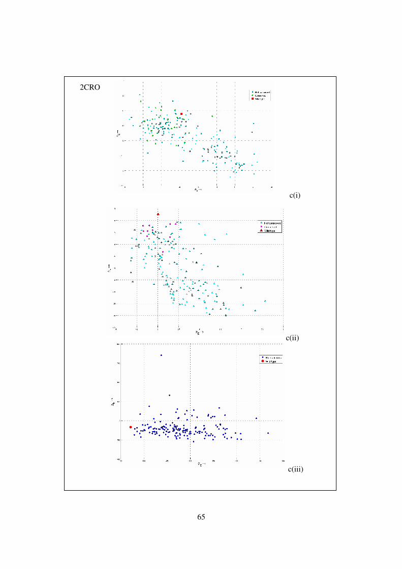
65

2CRO

c(i)

c(ii)

c(iii)

66

4ICB

d(i)

d(ii)

d(iii)

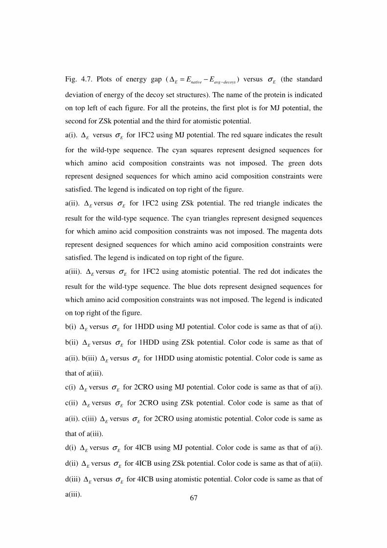
67

Fig. 4.7. Plots of energy gap (E native avg decoys

E E −∆ = − ) versus Eσ (the standard

deviation of energy of the decoy set structures). The name of the protein is indicated

on top left of each figure. For all the proteins, the first plot is for MJ potential, the

second for ZSk potential and the third for atomistic potential.

a(i). E∆ versus Eσ for 1FC2 using MJ potential. The red square indicates the result

for the wild-type sequence. The cyan squares represent designed sequences for

which amino acid composition constraints was not imposed. The green dots

represent designed sequences for which amino acid composition constraints were

satisfied. The legend is indicated on top right of the figure.

a(ii). E∆ versus Eσ for 1FC2 using ZSk potential. The red triangle indicates the

result for the wild-type sequence. The cyan triangles represent designed sequences

for which amino acid composition constraints was not imposed. The magenta dots

represent designed sequences for which amino acid composition constraints were

satisfied. The legend is indicated on top right of the figure.

a(iii). E∆ versus Eσ for 1FC2 using atomistic potential. The red dot indicates the

result for the wild-type sequence. The blue dots represent designed sequences for

which amino acid composition constraints was not imposed. The legend is indicated

on top right of the figure.

b(i) E∆ versus Eσ for 1HDD using MJ potential. Color code is same as that of a(i).

b(ii) E∆ versus

Eσ for 1HDD using ZSk potential. Color code is same as that of

a(ii). b(iii) E∆ versus Eσ for 1HDD using atomistic potential. Color code is same as

that of a(iii).

c(i) E∆ versus Eσ for 2CRO using MJ potential. Color code is same as that of a(i).

c(ii) E∆ versus Eσ for 2CRO using ZSk potential. Color code is same as that of

a(ii). c(iii) E∆ versus

Eσ for 2CRO using atomistic potential. Color code is same as

that of a(iii).

d(i) E∆ versus

Eσ for 4ICB using MJ potential. Color code is same as that of a(i).

d(ii) E∆ versus Eσ for 4ICB using ZSk potential. Color code is same as that of a(ii).

d(iii) E∆ versus

Eσ for 4ICB using atomistic potential. Color code is same as that of

a(iii).

68

always negative, i.e., the native state energy is less than the average of the decoy

structure energies for all the four proteins when we use the atomistic potential. This

implies that the wild-type sequence will favorably select the native structure over other

native-like structures. However, when we use the other potentials, we note that the energy

gap is not always negative for all the four proteins. We got negative energy gap for only

4ICB with the MJ potential, while negative energy gap was achieved for only 1FC2 with

ZSk potential. Thus, even though we are able to achieve convergence by keeping the

amino acid composition fixed for ensuring specificity while using MJ and ZSk potentials,

but are unable to do so while using atomistic potentials, the sequences designed using

atomistic potentials seem to be more appropriate as they satisfy the negative energy-gap

criterion. It is interesting to note that many of our designed sequences have energy gap

lower than that of the corresponding wild-type sequence. Some may find it surprising but

it is not uncommon in de novo protein design literature to come across works where

sequences have been redesigned to be more stable than their wild-type counterparts

(Chen et al., 2000, Dantas et al., 2003).

We also present the average time taken by IPOPT for designing sequences using

different potentials for all the four proteins in Table 4.2. Even though gradient-based

continuous optimization methods are computationally efficient in determining a local

minimum, the average time taken by IPOPT for designing sequences for the four proteins

(especially using atomistic potentials) is quite high in our opinion. In the next section, we

present the quadratic programming approach for designing sequences which is much

faster.

69

Table 4.2. Average time taken for designing sequences of each protein using MJ

(Miyazawa and Jernigan, 1996), ZSk (Zhang and Skolnick, 1998) and atomistic

potentials (Cornell at al., 1995, Fraternali and Gunsteren, 1996).

Protein PDB ID

and number of

residues

MJ ZSk Atomistic

1FC2 (chain C)

43 30 m 8 s 1 h 19 m 32 s 20 m 51 s

1HDD (chain C)

57 1h 36 m 2 s 2 h 55 s 3 h 36 m 2 s

2CRO

65 2 h 1 m 14 s 2 h 13 m 30 s 5 h 11 m 15 s

4ICB

76 3 h 12 m 10 s 2 h 51 m 21 s 6 h 4 m 58 s

4.3 The Quadratic Programming method

4.3.1 Method

In the quadratic programming approach, for an N residue protein we select a vector

20N∈x � with each element representing a particular amino acid at a particular position

in the sequence. Thus, at the thi residue position in the sequence, the th

m type of residue

will be identified by the element 20( 1)i mx − + of x . Hence, the dimension of x is 20 1N × .

The following ordering was used for the amino acids: {C M F I L V W Y A G T S N Q D

E H R K P}. The sequence design problem is formulated, following Koh et al. (2005) as

follows,

1Minimize

2T

E =x

x Qx (4.14)

Subject to =Bx c (4.15)

and 0 1 1, 20ix i N≤ ≤ ∀ =

where zero for an entry in x means vacancy at a corresponding site by a corresponding

amino acid residue and one implies occupancy at the same site by that particular residue.

70

Q is the energy matrix; the thij entry of Q gives the contact energy between the thi and

thj residues when the Cα atoms are within a contact distance of 7.0 Å of each other. The

contact energy consists of three atomistic potentials, namely, electrostatic, van der Waals

and solvation potentials. The atomistic electrostatic charges and van der Waals

parameters are taken from the AMBER force field (Cornell et al., 1995) and for solvation

energy, we use the implicit solvation energy model proposed by Fraternali and Gunsteren

(1996). The contact energy depends on the orientations of the side chains of the residues

in contact. We use SCWRL version 4 (2003) to determine the orientation of the side-

chains. SCWRL uses the backbone coordinates of each pair of interacting residues in the

native structure and gives the best side-chain orientation.

Based on assumptions stated above, the pair-wise contact energy is given by,

ij electrostatic VW solvation

Q E E E= + + if the thi and thj residues are in contact

= 0 otherwise

Thus, after expansion, Eq. 4.14 takes the following form

20 20

20( 1) 20( 1) ,20( 1) 20( 1)1 1 1 1

12

N N

i k i k j l j l

i j k l

E x Q x− + − + − + − += = = =

=

∑∑ ∑∑ (4.16)

where the indices i and j indicate the positions on the backbone that are in contact, and

the indices k and l indicate the type of amino acid at positions i and j respectively. B is

the constraint matrix and c the constraint vector. The first N rows of B and c indicate

the number of residues at any position on the backbone. Since, only one amino acid can

occupy a position on the backbone at a time, the first N rows of c are all ones. The thi

row of B ( i N≤ ) gives the coefficients of the variables { }x corresponding to the thi

position on the backbone; the only variables active at the thi position are from

20( 1) 1i − + to 20i . Thus for row i,

1ij

B = for 20( 1) 1 to 20j i i= − +

= 0 otherwise

Hence, the first N rows of the constraint eq. 4.4.2 can be written as

20

20( 1)1

1 for 1i j

j

x i N− +=

= ≤ ≤∑ (4.17)

71

The last 20 rows of B and c specify the amino acid composition of the sequence to be

designed. Thus, if the sequence to be designed should have five Glycines, then the

( )10th

N + row of c is equal to five (note that in the order of amino acids mentioned

above Glycine is at the 10th position). On the other hand, in the ( )10th

N + row of the left

hand side of Eq. 4.15, only variables corresponding to Glycine should be present. Hence,

every 10th element of B in the 10 thN + row should be one while the rest are zeroes.

Thus, the last 20 rows of the constraint Eq. 4.15 can be written as

20( 1)1

for 1 20N

j m m

j

x N m− +=

= ≤ ≤∑ (4.18)

where mN is the number of amino acids of type m. We also ensure that,

20

1m

m

N N=

=∑ (4.19)

because the sum of the number of different types of amino acids should add up to the

length of the sequence. From Eqs. 4.17 and 4.18 it is easy to see that the dimension of B

is (20 ) 20N N+ × and that of c is (20 ) 1N+ × .

We solve the optimization problem posed in Eqs. 4.14 and 4.15 by using the

interior point optimization method (IPOPT) (Wächter and Biegler, 2004) (refer Appendix

B1). Interior point optimization methods are efficient in handling a large number of

optimization variables, nonlinear objective function, and a large number of constraints.

As an example, for designing the smallest protein sequence which has 46 residues we

have 46 20 920× = design variables and 46 20 66+ = constraints along with the

optimization function given by Eq. 4.16. For such problems, IPOPT takes only six to

seven minutes on a Xeon 3.0 GHz desktop computer.

4.3.2 Results

Optimization using quadratic programming formulation is much faster compared to the

double sigmoid approach. We used quadratic programming on the same set of four

proteins in the FISA decoy set to design sequences. Based on these design criteria and

different initial values of the design variables x , we generate approximately 100

sequences for each protein structure. Table 4.3 gives the average time required for

72

Table 4.3 Average time taken to design sequences for each protein in the FISA decoy set

using quadratic programming formulation.

PDB ID Number of residues Average time

1FC2 (chain C) 43 7 m 39 s

1HDD (chain C) 57 16 m 47 s

2CRO 65 24 m 10.5 s

4ICB 76 46 m 30.5 s

designing set of sequences for each protein using quadratic programming formulation.

All the calculations were done in a Xeon 3.0 GHz quad-core desktop computer. As

before, we did not employ parallelization, so each calculation was done on one processor

at a time.

As explained in Section 4.3, we align the designed sequences with the wild-type

ones and also find matches with reduced set of five amino acid alphabets using the same

grouping schemes mentioned in section 4.3. We use the scoring scheme in Eq. 4.13 to

select the best designed sequences and present them in Fig. 4.8. The reduced amino acids

are represented by ‘A’, ‘B’, ‘C’, ‘D’ and ‘E’. When we align our maximum score

sequences with their wild-type counterparts by using the sequence alignment program

CLUSTAL version 1.83 (Higgins and Sharp, 1988) which allows gaps to be introduced in

the sequences, we notice that the number of matches increase. The results of CLUSTAL

alignment for the four proteins are shown in Fig. 4.9. As explained in Section 4.3, we

again test our designed sequences by threading them to the decoy structures in the FISA

decoy set and note the energy gaps and energy dispersions for these four proteins. The

results are presented in Fig. 4.10.

73

(a)

74

(b)

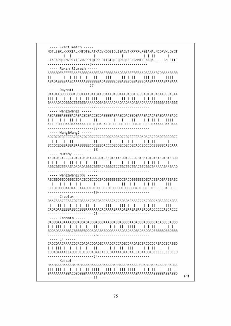
75

(c)

76

(d)

77

(a)

(b)

(d)

(c)

Fig. 4.8. The highest scoring designed sequences for the four proteins 1FC2 (chain

C), 1HDD (chain C), 2CRO and 4ICB. Each match is shown by a ‘|’ symbol. For

each protein, we first show the number of matches with all 20 amino acids which we

term as ‘exact match’, and then each five letter reduced amino acid sets denoted by

the corresponding authors. For every case, the top is the wild-type and the bottom

one is the designed sequence. The number of matches for each method is shown

below the each grouping scheme as well as the non-reduced one. Wang&Wang1,

Wang&Wang2 and Wand&Wang2002 refers (Wang and Wang, 1999 and Wang and

Wang, 2002) grouping schemes respectively.

(a) 1FC2 (chain C); 18.6 % amino acid matches without introducing gaps.

(b) 1HDD (chain C); 17.5 % amino acid matches without introducing gaps.

(c) 2CRO; 13.8 % amino acid matches without introducing gaps.

(d) 4ICB; 14.5 % amino acid matches without introducing gaps.

78

In Fig. 4.10, we note that energy gap, i.e., E native avg decoysE E −∆ = − is negative for all the

designed sequences (shown as blue stars) as well for the wild-type sequence (shown as a

red dot). Since, the free energy is always negative in sign, all our designed sequences as

well as the wild-type sequences satisfy the first criteria, i.e., the energy of the native

structure is lower than that of the decoy set structures. However, we see that the

dispersion in energy of the decoy structures is almost similar in magnitude as the energy

gap for 1FC2-C, 1HDD-C and 2CRO for the wild-type as well as the designed sequences.

Based on the definition of the Z-score (Shakhnovich and Gutin, 1993, Abkevich and

Shakhnovich, 1996) , i.e.,

_

_

decoy setnative

decoy set

E EZ

σ

−= (4.20)

we see that the dispersion in energy of the decoy structures is almost similar in magnitude

as the energy gap for 1FC2-C, 1HDD-C and 2CRO for the wild-type as well as the

designed sequences. Thus, for these three proteins 1Z ≈ , which is not encouraging from

the Z-score optimization point of view. This leaves the possibilities for improvement in

energy models and the implementation scheme which we discuss later. However, for the

other protein, 4ICB, we note that 4Z > for many designed sequences as well as for the

wild-type sequence. Thus, the designed sequences for this protein perfectly satisfies the

Z-score optimization criteria even though our sequence design method is not based on Z-

score optimization. As before, we note that some of the designed sequences are more

stable than the wild-type sequence based on the Z-score maximization criterion.

Fig. 4.9. Results of sequence alignment using sequence alignment program CLUSTAL

(version 1.83). ‘*’ denotes a match; ‘:’ denotes conserved substitution; ‘.’ denotes semi-

conserved substitution. ( http://www.ebi.ac.uk/help/formats.html ). As indicated, the top

sequence is the wild-type variety and the bottom the designed one.

(a) 1FC2 (b) 1HDD-C (c) 2CRO and (d) 4ICB.

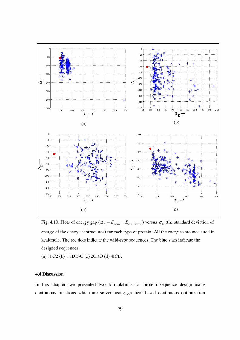
79

4.4 Discussion

In this chapter, we presented two formulations for protein sequence design using

continuous functions which are solved using gradient based continuous optimization

Fig. 4.10. Plots of energy gap ( E native avg decoysE E −∆ = − ) versus Eσ (the standard deviation of

energy of the decoy set structures) for each type of protein. All the energies are measured in

kcal/mole. The red dots indicate the wild-type sequences. The blue stars indicate the

designed sequences.

(a) 1FC2 (b) 1HDD-C (c) 2CRO (d) 4ICB.

(a) (b)

(c) (d)

80

methods. We now discuss a few merits and demerits of both the methods and also about

sequence design by free energy minimization using pair-wise contact potentials.

The double sigmoid method takes considerably more time (Table 4.2) than the

quadratic programming method (Table 4.3). Furthermore, with amino acid composition

constraints, especially with the atomistic potentials, the double sigmoid method was

unable to converge in many instances. On the other hand, the quadratic programming

method always converged with amino acid composition constraints using atomistic

potentials with different initial guesses. There is another inherent disadvantage of the

double sigmoid method; because of the nonconvexity on the energy surface it explores

(see Fig. 4.3), the solutions found by this method will depend on the contour of the

energy surface. Thus, if the energy surface profile is changed, which can be done by

altering the positions of amino acids, i.e., shifting rows and columns of the energy

matrices, the solutions found by the double sigmoid method will change for the same

initial inputs. Hence, the double sigmoid method is dependant on the order in which the

amino acids are presented in the energy matrices. As each amino acid represents a

separate design variable in the quadratic programming problem, no such problem will be

encountered. On the other hand, any value of the design variable between zero and

twenty represents an amino acid in the double sigmoid method; hence, whenever it

converges, it gives a specific sequence. However, in the quadratic programming

formulation, a specific amino acid is obtained only if the design variable corresponding to

it is one or near one (in our computer programs we kept this limit as greater than or equal

to 0.9). Hence, even though the quadratic programming method may converge obeying

all constraints, the final answer may not correspond to a protein sequence.

The present formulation based on pair-wise contact energies has a drawback when

we use atomistic potentials with implicit solvation model. Pair-wise energy calculation is

valid for electrostatic and van der Waals energies, but solvation energy depends upon

exposed surface area of the residues which is not pair-wise additive. Thus, the surface

area of a group of residues in close contact with one another is not equal to the sum of the

surface areas when two residues are taken at a time; in fact this leads to over-counting of

the surface area (Gordon and Mayo, 1999). One has to take all the atoms of all the

residues in contact simultaneously to calculate the surface area correctly. However,

81

determining the correct solvation energy by taking all residues together will lead to a high

increase in the computational cost. For example, if m residues are in contact with one

another, we now have 2

m

(i.e., ( )

!2 !2!

m

m −) contact energy matrices of size 20×20.

However, if we want to calculate all possible combinations of contact energies of 20

amino acids for such a m residue group we will have to calculate a 20×20×20×….×20

contact energy matrix of m dimensions which leads to an exponential increase in

dimensionality. The energy evaluation formula for the quadratic programming method

(eq. 4.4.3) will then be modified as,

1 1 2 2 1 2 2 2

1 2 1 2

20 20 20

20( 1) ,20( 1) ,....20( 1) 20( 1) 20( 1) 20( 1)1 1 1 1 1 1

1.... .... ....

2 m m m m

m m

N N N

m i k i k i k i k i k i k

i i i k k k

E Q x x x− + − + − + − + − + − += = = = = =

=

∑∑ ∑ ∑∑ ∑

for every m group of residues taken together, and there may be several such closely

packed groups in a protein.

4.5 Closure

In this chapter we presented two approaches for protein sequence design for fixed

backbone conformations. Both the methods minimize free energy to design sequences

which is posed as a continuous function and solved using gradient based optimization

methods. We also developed formulations to impose amino acid composition constraints

in the continuous optimization problem framework. We demonstrated the generality of

the methods by incorporating different potentials ranging from coarse-grained statistical

ones to atomistic, and use both the methods to design sequences for four proteins of

varying chain lengths. We further tested the designed sequences by matching them with

the wild-type ones and also checked for stability by calculating the energy gap and

dispersion in energies using the decoy sets available for the four proteins. We end by a

discussion on the merits and demerits of each method.

82

5. Search in the Conformation Space

• We explain our approach towards protein structure prediction from the point of its

application in simultaneous sequence and conformation search.

• We describe the formulation of a coarse-grained energy function from the MJ

matrix.

• We present a structure prediction formulation based on elastic network model and

show its application by taking examples of real proteins.

• We formulate a continuous coarse-grained energy function to form coarse-grained

models of secondary structures like alpha helix.

• We describe a coarse-grained tertiary structure prediction method with rigid

secondary structures and validate it using several proteins.

• We present a discussion on both the structure prediction methods and select one

of them for future use in simultaneous sequence and conformation search

application.

• We close the chapter by a brief summary.

5.1 Introduction

The work presented in this chapter is concerned with the search of the conformation

space of the designed sequences for minimum-energy conformations. Even though the

conformation of the protein molecule has to obey constraints within the limits of the

Ramachandran map, still the protein molecule can take an infinite number of

conformations in the three-dimensional space. Consequently, searching the

conformational space is a computational intensive task. Hence, our focus is on techniques

that are amenable for computationally efficient energy potentials. First, we present a

novel coarse-grained continuous energy function based on the MJ matrix (Miyazawa and

Jernigan, 1996). Then, we present two conformation search methods, both of which use

the OB-CG (One-Bead Coarse-Grained) model that we developed. The first conformation

search method that we developed is based on the elastic network model, which we

implemented in MATLAB. This model is applied on a few proteins that show

preliminary results starting from fully unfolded states of polypeptides. However, we have

83

not used it subsequently because of some issues which we discuss in the relevant section

on discussions about this method. We have tried to predict secondary structure formation

using continuous optimization and have been successful to formulate a continuous

function which can form OB-CG model of alpha-helices when optimized starting from a

fully unfolded state. We present a short section on the description of this method.

However, alpha helix formation does not take place when we incorporate this function

with other terms in the OB-CG model. Henceforth, we developed a simple chain/linkage

model that incorporates secondary structures such as alpha helices and beta strands as

rigid bodies. However, the formation of beta sheets by pairing of beta strands is a

combinatorial problem and is still open and is not addressed using gradient based

continuous optimization. The chain/linkage model with pre-specified rigid secondary

structures works well with alpha-helical proteins in predicting tertiary structures from

unfolded states. To increase the computational efficiency, we developed our own

nonlinear conjugate gradient program and implemented the chain/linkage model using

C++ language (Please refer to Appendix B3 to see the algorithm). The results of this

method are given for some alpha helical proteins of different chain lengths. We also

present a case where this method is used for ab intio structure prediction with sequence

information only. We have used this method in our simultaneous sequence and

conformation search method presented in Chapter 6 of this thesis.

5.2 Coarse-grained energy function formulation

We use the latest MJ matrix (Miyazawa and Jernigan, 1996) to get the energy of

interaction between two non-bonded but interacting residues. Two non-bonded residues

are said to be interacting when they are within a distance of 6.5 Å from each other.

Since our model is based on MJ matrix, we want to make our energy model closely

follow the limits of the MJ matrix. Thus, the contact energy ijE between the thi and thj

non-bonded interacting residues in our coarse-grained model should be equal to the value

in the MJ matrix for the corresponding pair of residues at thi and thj positions. We have

modeled this using a sigmoid function which is the 1st term on the right hand side of Eq.

5.1. However, this does not prevent two residues from coming too close and even

overlapping on one another. To prevent this unrealistic scenario, we add a parabolic

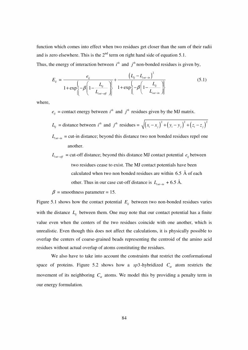
84

function which comes into effect when two residues get closer than the sum of their radii

and is zero elsewhere. This is the 2nd term on right hand side of equation 5.1.

Thus, the energy of interaction between thi and thj non-bonded residues is given by,

ijE = ( )

2

1 exp 11 exp 1

ij cut inij

ijij

cut incut off

L Le

LL

LLββ

−

−−

−+

+ − −+ − −

(5.1)

where,

ije = contact energy between thi and thj residues given by the MJ matrix.

ijL = distance between thi and thj residues = ( ) ( ) ( )

2 2 2

i j i j i jx x y y z z− + − + −

cut inL − = cut-in distance; beyond this distance two non bonded residues repel one

another.

cut offL − = cut-off distance; beyond this distance MJ contact potential ije between

two residues cease to exist. The MJ contact potentials have been

calculated when two non bonded residues are within 6.5 Å of each

other. Thus in our case cut-off distance is cut inL − + 6.5 Å.

β = smoothness parameter = 15.

Figure 5.1 shows how the contact potential ijE between two non-bonded residues varies

with the distance ijL between them. One may note that our contact potential has a finite

value even when the centers of the two residues coincide with one another, which is

unrealistic. Even though this does not affect the calculations, it is physically possible to

overlap the centers of coarse-grained beads representing the centroid of the amino acid

residues without actual overlap of atoms constituting the residues.

We also have to take into account the constraints that restrict the conformational

space of proteins. Figure 5.2 shows how a 3sp -hybridized Cα atom restricts the

movement of its neighboring Cα atoms. We model this by providing a penalty term in

our energy formulation.

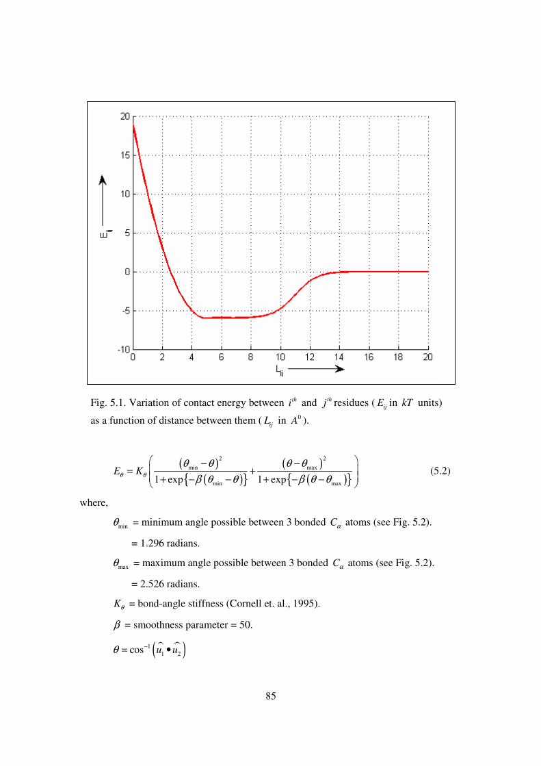
85

( )

( ){ }( )

( ){ }

2 2

min max

min max1 exp 1 expE Kθ θ

θ θ θ θ

β θ θ β θ θ

− −= +

+ − − + − − (5.2)

where,

minθ = minimum angle possible between 3 bonded Cα atoms (see Fig. 5.2).

= 1.296 radians.

maxθ = maximum angle possible between 3 bonded Cα atoms (see Fig. 5.2).

= 2.526 radians.

Kθ = bond-angle stiffness (Cornell et. al., 1995).

β = smoothness parameter = 50.

� �( )11 2cos u uθ −= •

Fig. 5.1. Variation of contact energy between thi and thj residues ( ijE in kT units)

as a function of distance between them ( ijL in 0A ).

86

and �1u and �2u are the unit vectors joining thi and ( 1)th

i − Cα atoms and thi and ( 1)th

i +

Cα atoms respectively. Figure 5.3 shows how the penalty term Eθ for the angle varies as

bond angle θ changes for three bonded Cα atoms. We incorporate another penalty term

to prevent the violation of the fixed bond-length between any two bonded Cα atoms. This

is done using the following function:

( )2

0bonded b ijE K L L= − (5.3)

where,

bK = bond length stiffness (Cornell et. al., 1995).

ijL = distance between th

i and thj bonded Cα atoms.

0L = equilibrium distance two bonded Cα atoms.

= 3.8 Å.

Fig. 5.2. The limits of angle θ between three adjacent Cα atoms. R (magenta

colored dots) represents a residue, CaCa the Cα atom, N (blue colored dots) for

Nitrogen and Coxy the Carboxyl Carbon atom. The Cα atoms on the ends can take

positions within the green cones only. This is due to the 3sp hybrid state of the Cα

atom at the center.

minθ

maxθ

φψ

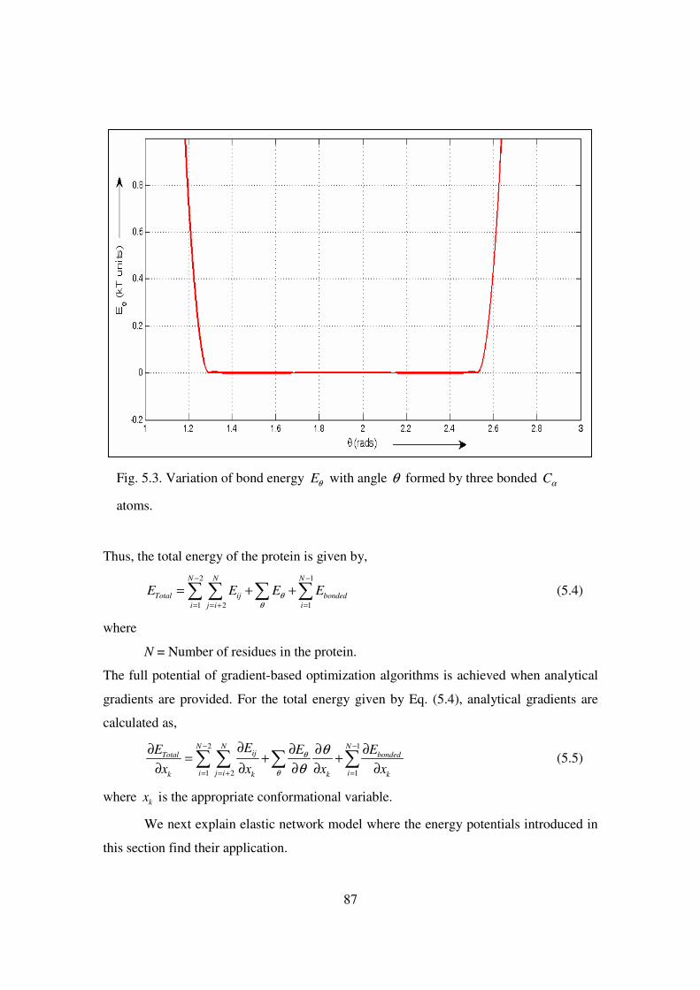
87

Thus, the total energy of the protein is given by,

2 1

1 2 1

N N N

Total ij bonded

i j i i

E E E Eθθ

− −

= = + =

= + +∑ ∑ ∑ ∑ (5.4)

where

N = Number of residues in the protein.

The full potential of gradient-based optimization algorithms is achieved when analytical

gradients are provided. For the total energy given by Eq. (5.4), analytical gradients are

calculated as,

2 1

1 2 1

N N NijTotal bonded

i j i ik k k k

EE E E

x x x x

θ

θ

θ

θ

− −

= = + =

∂∂ ∂ ∂∂= + +

∂ ∂ ∂ ∂ ∂∑ ∑ ∑ ∑ (5.5)

where kx is the appropriate conformational variable.

We next explain elastic network model where the energy potentials introduced in

this section find their application.

Fig. 5.3. Variation of bond energy Eθ with angle θ formed by three bonded Cα

atoms.

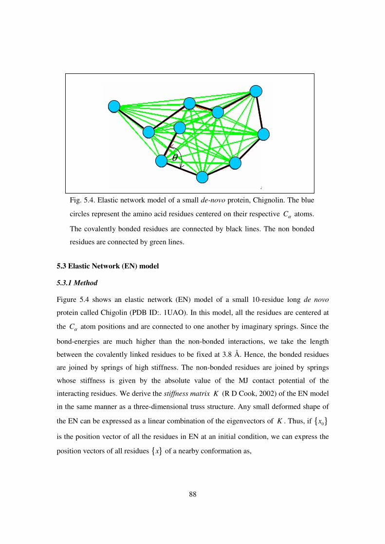
88

5.3 Elastic Network (EN) model

5.3.1 Method

Figure 5.4 shows an elastic network (EN) model of a small 10-residue long de novo

protein called Chigolin (PDB ID:. 1UAO). In this model, all the residues are centered at

the Cα atom positions and are connected to one another by imaginary springs. Since the

bond-energies are much higher than the non-bonded interactions, we take the length

between the covalently linked residues to be fixed at 3.8 Å. Hence, the bonded residues

are joined by springs of high stiffness. The non-bonded residues are joined by springs

whose stiffness is given by the absolute value of the MJ contact potential of the

interacting residues. We derive the stiffness matrix K (R D Cook, 2002) of the EN model

in the same manner as a three-dimensional truss structure. Any small deformed shape of

the EN can be expressed as a linear combination of the eigenvectors of K . Thus, if { }0x

is the position vector of all the residues in EN at an initial condition, we can express the

position vectors of all residues { }x of a nearby conformation as,

Fig. 5.4. Elastic network model of a small de-novo protein, Chignolin. The blue

circles represent the amino acid residues centered on their respective Cα atoms.

The covalently bonded residues are connected by black lines. The non bonded

residues are connected by green lines.

θ

89

{ } { } { }3

01

N

i i

i

x x α ω=

= +∑ (5.6)

where,

N = number of residues in the polypeptide.

{ }x = column vector of Cartesian coordinates of all Cα atoms; so its dimension is

3 1N × .

{ } = th

i iω eigenvector of K with dimension 3 1N × .

iα = scalar multiplier associated with thi eigenvector { }iω .

The scalar multipliers { }iα form the set of design variables in our optimization problem

formulation. By varying these coefficients, we change the conformation; and with it the

energy of the polypeptide. This method allows only small changes in conformation

because eigenvector decomposition is restricted to the linear regime. To apply this

method for large changes in conformation, we formulate a novel algorithm which updates

the stiffness matrix of EN of the polypeptide from time to time as optimization

progresses. This algorithm is shown in Fig. 5.5. It is implemented in MATLAB and uses

the optimization toolbox fminunc. As explained in Fig. 5.5, the rate at which we update

the stiffness matrix K is determined by the maximum number of iterations (maxiter)

specified in the optimization program. In Fig. 5.6 we show, for different values of

maxiter, how conformational energy of Chignolin varies with iteration as we minimize

the energy from a fully unfolded state. Table 5.1 compares the energy of the final

conformation, total number of iterations and actual cpu time for different values of

maxiter. It is interesting to note that the energy of the optimal conformation shows

insignificant change as maxiter is varied, as shown in Table 5.1. Even when we do not

update the stiffness matrix at all, the change in optimal value of the energy is very low.

To save time in the case of large polypeptides, one could perform the optimization

without updating K . In such case, one can think of using the eigenvectors as basis

90

Fig. 5.5. Flowchart showing our algorithm for large change in conformation

determined using eigenvectors of stiffness matrix K of EN.

No

Initial conformation: fully stretched polypeptide. Form the stiffness matrix K . Set tolerance =ε . Set initial guess of { }iα s.

Set maximum number of iterations (maxiter) for optimization program fminunc after which K is updated. Calculate energy E . Set E to some very large value.

Run optimization program fminunc. New energy = newE .

Update K with new { }iα s.

Update old energy

newE E= newE E ε− > Yes

Stop iterations. Final energy =

newE .

{ }i newα and eigenvectors of newK define final

conformation.

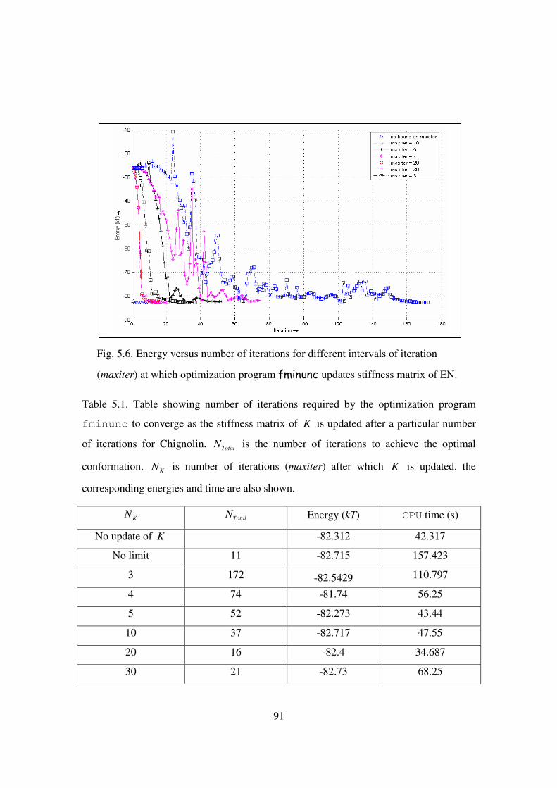
91

Table 5.1. Table showing number of iterations required by the optimization program

fminunc to converge as the stiffness matrix of K is updated after a particular number

of iterations for Chignolin. TotalN is the number of iterations to achieve the optimal

conformation. KN is number of iterations (maxiter) after which K is updated. the

corresponding energies and time are also shown.

KN TotalN Energy (kT) CPU time (s)

No update of K -82.312 42.317

No limit 11 -82.715 157.423

3 172 -82.5429 110.797

4 74 -81.74 56.25

5 52 -82.273 43.44

10 37 -82.717 47.55

20 16 -82.4 34.687

30 21 -82.73 68.25

Fig. 5.6. Energy versus number of iterations for different intervals of iteration

(maxiter) at which optimization program fminunc updates stiffness matrix of EN.

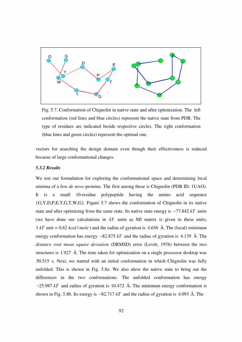
92

vectors for searching the design domain even though their effectiveness is reduced

because of large conformational changes.

5.3.2 Results

We test our formulation for exploring the conformational space and determining local

minima of a few de novo proteins. The first among these is Chignolin (PDB ID: 1UAO).

It is a small 10-residue polypeptide having the amino acid sequence

{G,Y,D,P,E,T,G,T,W,G}. Figure 5.7 shows the conformation of Chignolin in its native

state and after optimizing from the same state. Its native state energy is 77.842 kT− units

(we have done our calculations in kT units as MJ matrix is given in these units;

1 unit = 0.62 /kT kcal mole ) and the radius of gyration is 4.656 Å. The (local) minimum

energy conformation has energy 82.875 kT− and the radius of gyration is 4.139 Å. The

distance root mean square deviation (DRMSD) error (Levitt, 1976) between the two

structures is 1.927 Å. The time taken for optimization on a single processor desktop was

50.515 s. Next, we started with an initial conformation in which Chignolin was fully

unfolded. This is shown in Fig. 5.8a. We also show the native state to bring out the

differences in the two conformations. The unfolded conformation has energy

25.987 kT− and radius of gyration is 10.472 Å. The minimum energy conformation is

shown in Fig. 5.8b. Its energy is 82.717 kT− and the radius of gyration is 4.093 Å. The

Fig. 5.7. Conformation of Chignolin in native state and after optimization. The left

conformation (red lines and blue circles) represent the native state from PDB. The

type of residues are indicated beside respective circles. The right conformation

(blue lines and green circles) represent the optimal one.

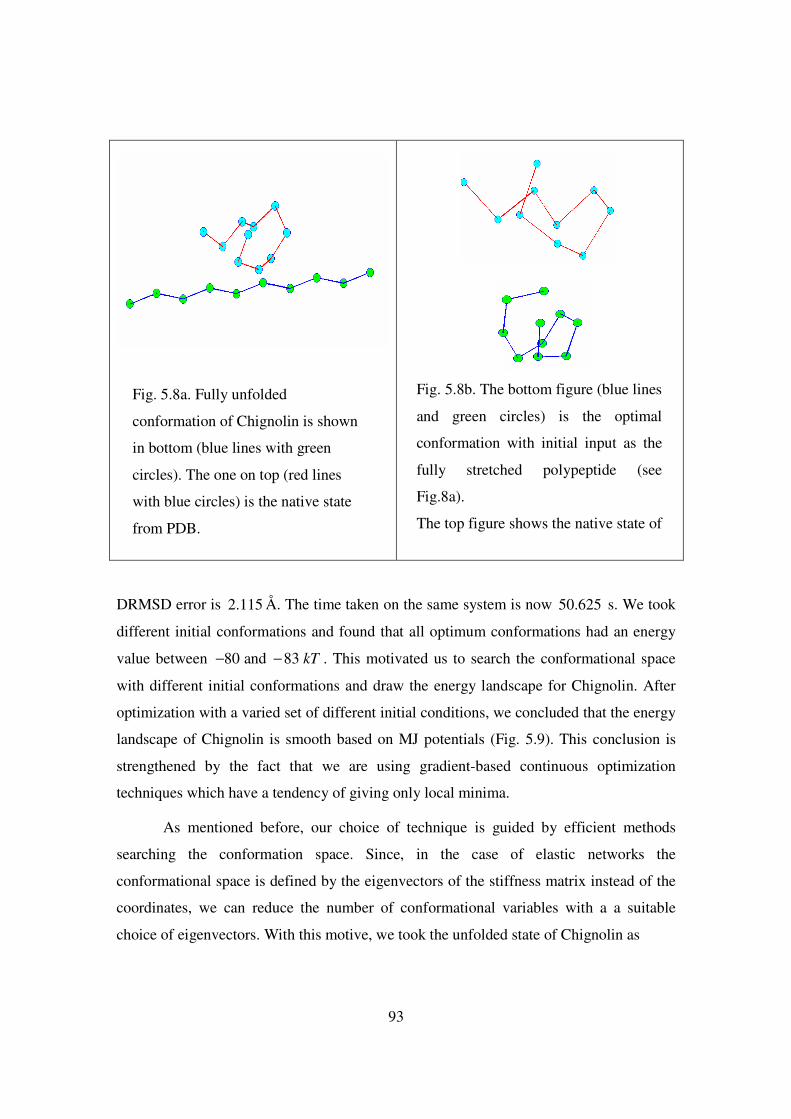
93

DRMSD error is 2.115 Å. The time taken on the same system is now 50.625 s. We took

different initial conformations and found that all optimum conformations had an energy

value between 80 and 83 kT− − . This motivated us to search the conformational space

with different initial conformations and draw the energy landscape for Chignolin. After

optimization with a varied set of different initial conditions, we concluded that the energy

landscape of Chignolin is smooth based on MJ potentials (Fig. 5.9). This conclusion is

strengthened by the fact that we are using gradient-based continuous optimization

techniques which have a tendency of giving only local minima.

As mentioned before, our choice of technique is guided by efficient methods

searching the conformation space. Since, in the case of elastic networks the

conformational space is defined by the eigenvectors of the stiffness matrix instead of the

coordinates, we can reduce the number of conformational variables with a a suitable

choice of eigenvectors. With this motive, we took the unfolded state of Chignolin as

Fig. 5.8b. The bottom figure (blue lines

and green circles) is the optimal

conformation with initial input as the

fully stretched polypeptide (see

Fig.8a).

The top figure shows the native state of

Fig. 5.8a. Fully unfolded

conformation of Chignolin is shown

in bottom (blue lines with green

circles). The one on top (red lines

with blue circles) is the native state

from PDB.

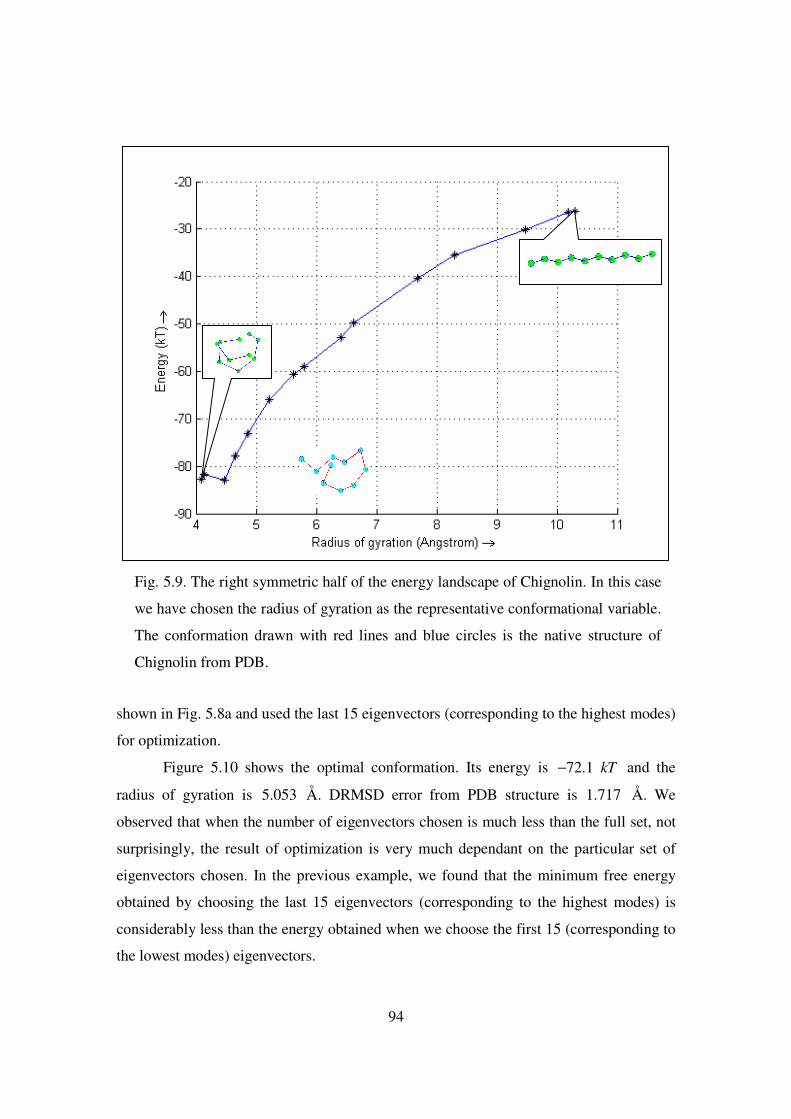
94

shown in Fig. 5.8a and used the last 15 eigenvectors (corresponding to the highest modes)

for optimization.

Figure 5.10 shows the optimal conformation. Its energy is 72.1 kT− and the

radius of gyration is 5.053 Å. DRMSD error from PDB structure is 1.717 Å. We

observed that when the number of eigenvectors chosen is much less than the full set, not

surprisingly, the result of optimization is very much dependant on the particular set of

eigenvectors chosen. In the previous example, we found that the minimum free energy

obtained by choosing the last 15 eigenvectors (corresponding to the highest modes) is

considerably less than the energy obtained when we choose the first 15 (corresponding to

the lowest modes) eigenvectors.

Fig. 5.9. The right symmetric half of the energy landscape of Chignolin. In this case

we have chosen the radius of gyration as the representative conformational variable.

The conformation drawn with red lines and blue circles is the native structure of

Chignolin from PDB.

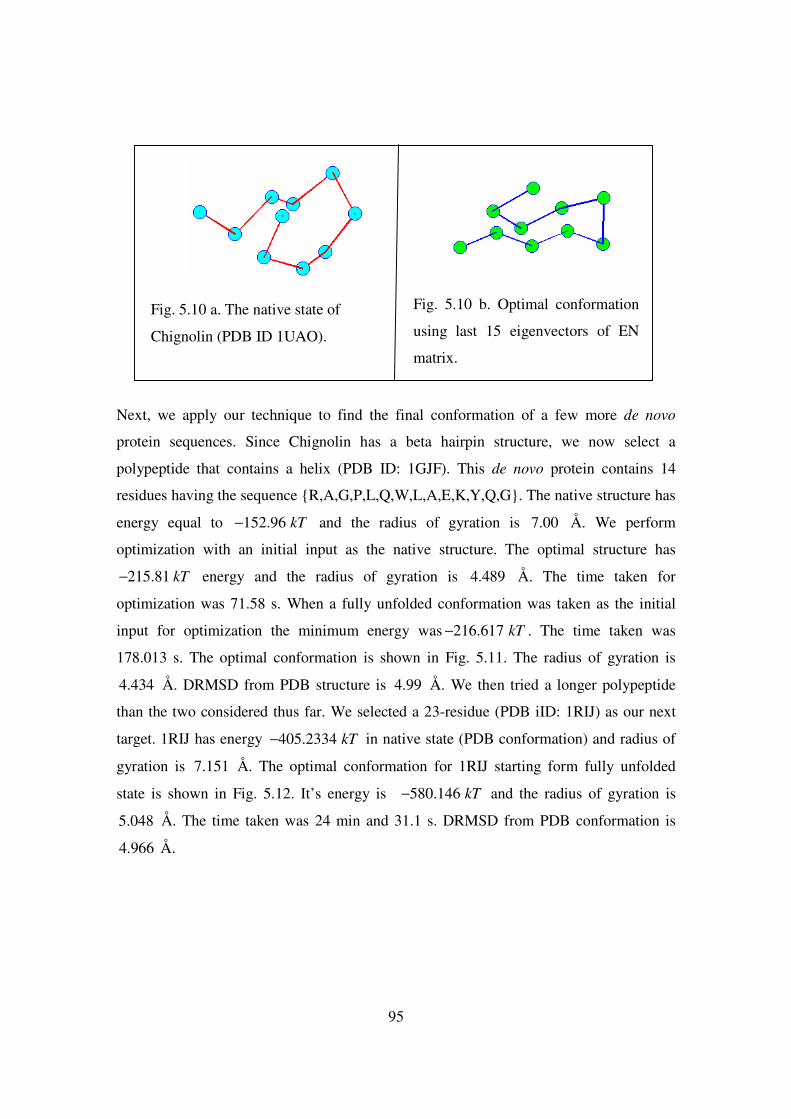
95

Next, we apply our technique to find the final conformation of a few more de novo

protein sequences. Since Chignolin has a beta hairpin structure, we now select a

polypeptide that contains a helix (PDB ID: 1GJF). This de novo protein contains 14

residues having the sequence {R,A,G,P,L,Q,W,L,A,E,K,Y,Q,G}. The native structure has

energy equal to 152.96 kT− and the radius of gyration is 7.00 Å. We perform

optimization with an initial input as the native structure. The optimal structure has

215.81 kT− energy and the radius of gyration is 4.489 Å. The time taken for

optimization was 71.58 s. When a fully unfolded conformation was taken as the initial

input for optimization the minimum energy was 216.617 kT− . The time taken was

178.013 s. The optimal conformation is shown in Fig. 5.11. The radius of gyration is

4.434 Å. DRMSD from PDB structure is 4.99 Å. We then tried a longer polypeptide

than the two considered thus far. We selected a 23-residue (PDB iID: 1RIJ) as our next

target. 1RIJ has energy 405.2334 kT− in native state (PDB conformation) and radius of

gyration is 7.151 Å. The optimal conformation for 1RIJ starting form fully unfolded

state is shown in Fig. 5.12. It’s energy is 580.146 kT− and the radius of gyration is

5.048 Å. The time taken was 24 min and 31.1 s. DRMSD from PDB conformation is

4.966 Å.

Fig. 5.10 b. Optimal conformation

using last 15 eigenvectors of EN

matrix.

Fig. 5.10 a. The native state of

Chignolin (PDB ID 1UAO).

96

Fig. 5.11a. PDB structure of 1GJF. Fig. 5.11b. Optimal structure of

1GJF from fully unfolded state.

Fig. 5.12 a. Native structure (PDB)

of 1RIJ.

Fig. 5.12 b. Optimal structure of

1RIJ from fully unfolded state.

97

We now take two natural proteins, namely, Ubiquitin (PDB ID: 1UBQ) with 76 residues,

and Lysozyme with 164 residues. Since, there was not much difference in results even

when K was not updated periodically, for these two cases we applied optimization

without updating K in order to save time. As discussed earlier, we can take the

eigenvectors of K as the basis vectors of the conformation space. When we perform

optimization in this space, there was no need to change the basis vectors of the space. The

optimal conformation and the native state of Ubiquitin from PDB are shown in Fig. 5.13.

Time taken for optimization was 23 h 29 m and 32 s. The energy of native conformation

was 2245.3 kT− with the radius of gyration equal to 11.493 Å. The energy after

optimization is 6830.5 kT− and radius of gyration is 5.576 Å. RMSD error from PDB

structure is 9.142 Å. The PDB conformation of Ubiquitin is far away from what we got

as the local minimum-energy conformation. We observe that our conformation is much

more compact than the PDB structure. This is because in the optimal conformation we do

not have secondary structures such as alpha helices and beta sheets. Secondary structures

Fig. 5.13 a. PDB structure of

Ubiquitin; the secondary structures

have been shown with bold lines.

Fig. 5.13 b. Conformation after

minimization of energy from native

state.

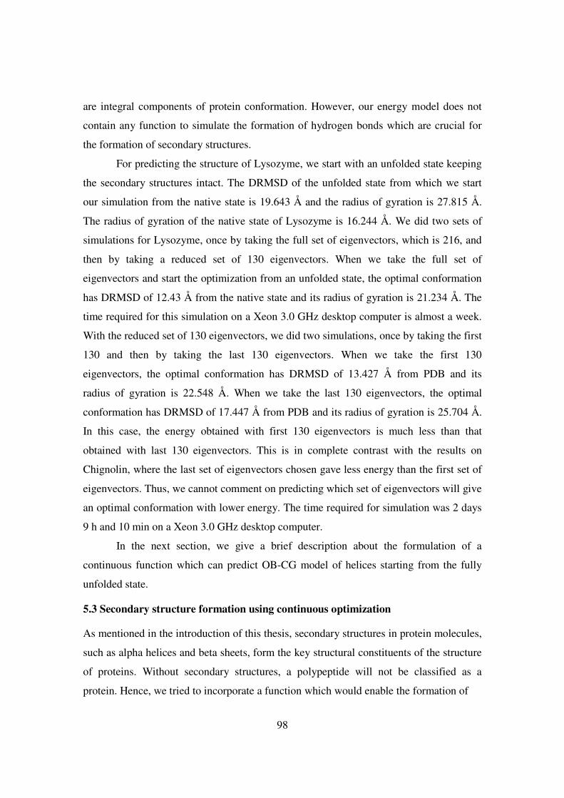
98

are integral components of protein conformation. However, our energy model does not

contain any function to simulate the formation of hydrogen bonds which are crucial for

the formation of secondary structures.

For predicting the structure of Lysozyme, we start with an unfolded state keeping

the secondary structures intact. The DRMSD of the unfolded state from which we start

our simulation from the native state is 19.643 Å and the radius of gyration is 27.815 Å.

The radius of gyration of the native state of Lysozyme is 16.244 Å. We did two sets of

simulations for Lysozyme, once by taking the full set of eigenvectors, which is 216, and

then by taking a reduced set of 130 eigenvectors. When we take the full set of

eigenvectors and start the optimization from an unfolded state, the optimal conformation

has DRMSD of 12.43 Å from the native state and its radius of gyration is 21.234 Å. The

time required for this simulation on a Xeon 3.0 GHz desktop computer is almost a week.

With the reduced set of 130 eigenvectors, we did two simulations, once by taking the first

130 and then by taking the last 130 eigenvectors. When we take the first 130

eigenvectors, the optimal conformation has DRMSD of 13.427 Å from PDB and its

radius of gyration is 22.548 Å. When we take the last 130 eigenvectors, the optimal

conformation has DRMSD of 17.447 Å from PDB and its radius of gyration is 25.704 Å.

In this case, the energy obtained with first 130 eigenvectors is much less than that

obtained with last 130 eigenvectors. This is in complete contrast with the results on

Chignolin, where the last set of eigenvectors chosen gave less energy than the first set of

eigenvectors. Thus, we cannot comment on predicting which set of eigenvectors will give

an optimal conformation with lower energy. The time required for simulation was 2 days

9 h and 10 min on a Xeon 3.0 GHz desktop computer.

In the next section, we give a brief description about the formulation of a

continuous function which can predict OB-CG model of helices starting from the fully

unfolded state.

5.3 Secondary structure formation using continuous optimization

As mentioned in the introduction of this thesis, secondary structures in protein molecules,

such as alpha helices and beta sheets, form the key structural constituents of the structure

of proteins. Without secondary structures, a polypeptide will not be classified as a

protein. Hence, we tried to incorporate a function which would enable the formation of

99

secondary structures based on our coarse-grained model. The following is a continuous

function which when optimized with respect to the conformation variables (the

coordinates of the residues) forms a helix from a fully unfolded polypeptide.

( ){ } ( )4

22 cos( ), 4

1 1

h

k

N N

HB HB k HB i i p

k i

E e e e L Lθ

θθ ω−

−

+= =

= − + + −∑ ∑ (5.7)

where,

HBe = strength of hydrogen bond in alpha helices (Arora and Jayram, 1997).

kθ = the kth dihedral angle between the planes formed by Cα atoms i, i+1, i+2 and

i+1, i+2, i+3 (Fig. 5.14).

ω = ideal coarse grained dihedral angle to form alpha helices (Tozzini and

Rocchia, 2006).

Fig. 5.14. Schematic diagram of an alpha helix; the Cα atoms are shown as black

dots. The bonds facing the viewer are drawn in thick black lines and the ones away

from the viewer are drawn dotted. �1v is the unit vector normal to the plane formed

by the i, i+1 and i+2 Cα atoms. �2v is the unit vector normal to the plane formed by

the i+1, i+2 and i+3 Cα atoms.

i +2

i

i +1

i +3

�1v

�2v

i +4

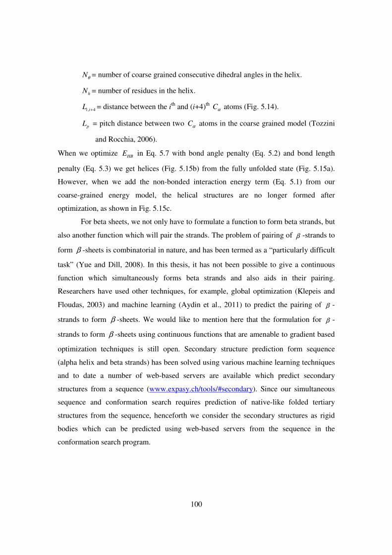
100

Nθ = number of coarse grained consecutive dihedral angles in the helix.

hN = number of residues in the helix.

, 4i iL + = distance between the ith and (i+4)th Cα atoms (Fig. 5.14).

pL = pitch distance between two Cα atoms in the coarse grained model (Tozzini

and Rocchia, 2006).

When we optimize HBE in Eq. 5.7 with bond angle penalty (Eq. 5.2) and bond length

penalty (Eq. 5.3) we get helices (Fig. 5.15b) from the fully unfolded state (Fig. 5.15a).

However, when we add the non-bonded interaction energy term (Eq. 5.1) from our

coarse-grained energy model, the helical structures are no longer formed after

optimization, as shown in Fig. 5.15c.

For beta sheets, we not only have to formulate a function to form beta strands, but

also another function which will pair the strands. The problem of pairing of β -strands to

form β -sheets is combinatorial in nature, and has been termed as a “particularly difficult

task” (Yue and Dill, 2008). In this thesis, it has not been possible to give a continuous

function which simultaneously forms beta strands and also aids in their pairing.

Researchers have used other techniques, for example, global optimization (Klepeis and

Floudas, 2003) and machine learning (Aydin et al., 2011) to predict the pairing of β -

strands to form β -sheets. We would like to mention here that the formulation for β -

strands to form β -sheets using continuous functions that are amenable to gradient based

optimization techniques is still open. Secondary structure prediction form sequence

(alpha helix and beta strands) has been solved using various machine learning techniques

and to date a number of web-based servers are available which predict secondary

structures from a sequence (www.expasy.ch/tools/#secondary). Since our simultaneous

sequence and conformation search requires prediction of native-like folded tertiary

structures from the sequence, henceforth we consider the secondary structures as rigid

bodies which can be predicted using web-based servers from the sequence in the

conformation search program.

101

b

a

c

Fig. 5.15. OB-CG model of alpha-helix starting from fully unfolded state.

a) An unfolded polypeptide.

b) OB-CG model of alpha helix after optimization of the function given by (5.2) +

(5.3) + (5.6) starting from the unfolded state shown in (a).

c) OB-CG model of alpha helix after optimization of the function given by (5.1) +

(5.2) + (5.3) + (5.6) starting from the unfolded state shown in (a).

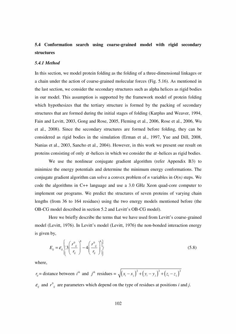
102

5.4 Conformation search using coarse-grained model with rigid secondary

structures

5.4.1 Method

In this section, we model protein folding as the folding of a three-dimensional linkages or

a chain under the action of coarse-grained molecular forces (Fig. 5.16). As mentioned in

the last section, we consider the secondary structures such as alpha helices as rigid bodies

in our model. This assumption is supported by the framework model of protein folding

which hypothesizes that the tertiary structure is formed by the packing of secondary

structures that are formed during the initial stages of folding (Karplus and Weaver, 1994,

Fain and Levitt, 2003, Gong and Rose, 2005, Fleming et al., 2006, Rose et al., 2006, Wu

et al., 2008). Since the secondary structures are formed before folding, they can be

considered as rigid bodies in the simulation (Erman et al., 1997, Yue and Dill, 2008,

Nanias et al., 2003, Sancho et al., 2004). However, in this work we present our result on

proteins consisting of only α -helices in which we consider the α -helices as rigid bodies.

We use the nonlinear conjugate gradient algorithm (refer Appendix B3) to

minimize the energy potentials and determine the minimum energy conformations. The

conjugate gradient algorithm can solve a convex problem of n variables in O(n) steps. We

code the algorithms in C++ language and use a 3.0 GHz Xeon quad-core computer to

implement our programs. We predict the structures of seven proteins of varying chain

lengths (from 36 to 164 residues) using the two energy models mentioned before (the

OB-CG model described in section 5.2 and Levitt’s OB-CG model).

Here we briefly describe the terms that we have used from Levitt’s coarse-grained

model (Levitt, 1976). In Levitt’s model (Levitt, 1976) the non-bonded interaction energy

is given by,

8 60 0

3 4ij ij

ij ij

ij ij

r rE

r rε

= −

(5.8)

where,

ijr = distance between thi and th

j residues = ( ) ( ) ( )2 2 2

i j i j i jx x y y z z− + − + −

ijε and 0ijr are parameters which depend on the type of residues at positions i and j.

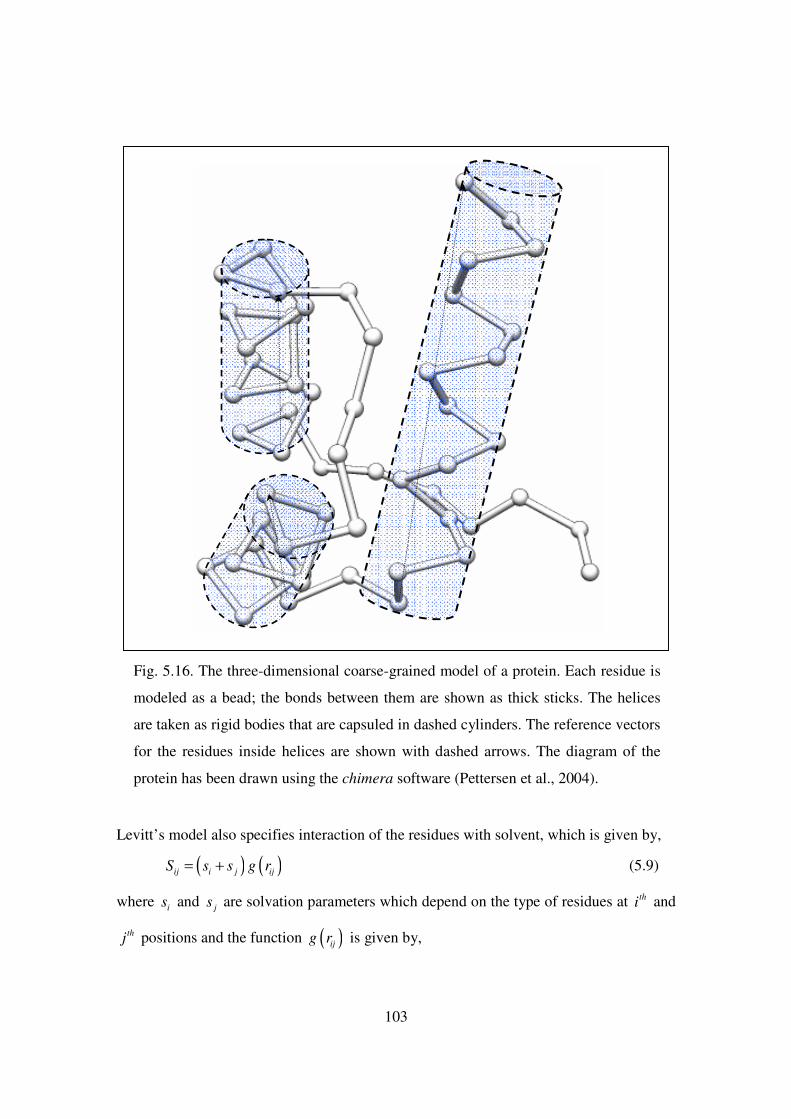
103

Levitt’s model also specifies interaction of the residues with solvent, which is given by,

( ) ( )ij i j ijS s s g r= + (5.9)

where is and

js are solvation parameters which depend on the type of residues at thi and

thj positions and the function ( )ijg r is given by,

Fig. 5.16. The three-dimensional coarse-grained model of a protein. Each residue is

modeled as a bead; the bonds between them are shown as thick sticks. The helices

are taken as rigid bodies that are capsuled in dashed cylinders. The reference vectors

for the residues inside helices are shown with dashed arrows. The diagram of the

protein has been drawn using the chimera software (Pettersen et al., 2004).

104

( ) ( )2 4 6 811 7 9 5

2ijg r x x x x= − − + − for 1x < (5.10)

0= for 1x ≥

where

9.0

ijrx =

Thus, the non-bonded energy using Levitt’s potential is given by ij ijE S+ . We have

omitted other terms in Levitt’s potential as those are not amenable to our OB-CG model.

5.4.2 Results

We take a set of seven proteins of different chain lengths to test the efficacy of the

gradient-based optimization method in predicting possible native-like protein structures.

The PDB IDs of each protein with the corresponding number of residues are given in

Table 5.2. Since, the optimization function (Eq. 5.4) is nonconvex, there ought to be

multiple minima. However, gradient-based optimization methods, even though very

efficient in determining local minima, cannot escape from a local minimum. Hence, we

search for minimum conformations using different initial structures (inputs to

optimization), i.e., structures which obey the constraints of the protein backbone (bond

length and angle constraints) but are conformationally well stretched as compared to the

native state, which is compact. We used 50-60 initial structures for proteins with residues

less than 50, 30-40 initial structures for proteins with residues between 50 and 100, and

20-25 initial structures for roteins with residues greater than 100.

Figure 5.17 shows the predicted structure of a protein with 81 residues (PDB ID:

1LRE). On the left hand side of the figure we show the predicted backbones using our

OB-CG potential (Fig. 5.17b) and Levitt (Fig. 5.17c) as also the native structure from

PDB (Fig. 5.17a). Since we have considered the α -helices as rigid bodies in our model,

the same are indicated with a different color (blue) on the backbone of the protein. As it

is difficult to understand the similarities/differences between three-dimensional chains of

proteins on a two-dimensional plane, we also show the contact map for each structure on

the right hand side. On the contact map, we consider the residue numbers along the X and

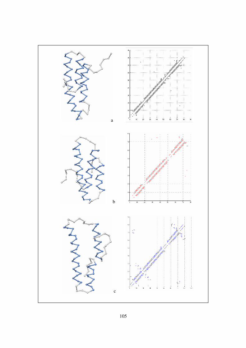
105

a

c

b

106

Y axes. If two non-bonded residues are within a particular distance (the contact distance,

which we take as 6.5 Å based on the MJ matrix) from each other a dot is placed on the

map at the corresponding position. For example, if residues i and j are within contact

distance, then we place a dot at the positions (i,j) and (j,i) on the map. The contact map is

very helpful in noting non-bonded residues which are far apart along the length of the

chain, but are in close proximity spatially. Such contacts indicate favorable interaction

among residues and are crucial in determining the tertiary or quaternary structure of the

protein. It is interesting to note that the α -helices appear as bands placed along the

diagonal in the contact maps (Figs. 5.17a, 5.17b, and 5.17c).

Table 5.2 shows the results of predicted structures for all the proteins. The first

column indicates the PDB ID, the number of residues in the protein, and also the

percentage of residues that are in the secondary structures, namely the α -helices. We do

this so that the reader can appreciate the simplification in computation once the α -

helices are assumed as rigid bodies in the simulation. In Table 5.2, we show the

DRMSDs for the predicted structure of each protein from corresponding native structures

Fig. 5.17. Predicted and native state structures of the protein with PDB id. 1LRE (81

residues). On the left hand side, we show the coarse-grained representation of the

protein (made with chimera), in which each residue is shown as a bead on the

backbone. The alpha helices are colored blue. On the right hand side we show the

corresponding contact map for the structure. Two non-bonded residues are taken to

be in contact if they are within a distance of 6.5 Å from each other. The contact

maps have been drawn using MATLAB software.

a) Native structure of the protein with PDB ID 1LRE. The contact map is shown on

the right hand side with black colored dots.

b) Minimum energy structure of the same protein using our OB-CG function. The

contact map is shown on the right hand side with red colored dots.

c) Minimum energy structure of the same protein using Levitt’s potential. The

contact map is shown on the right hand side with blue colored dots.

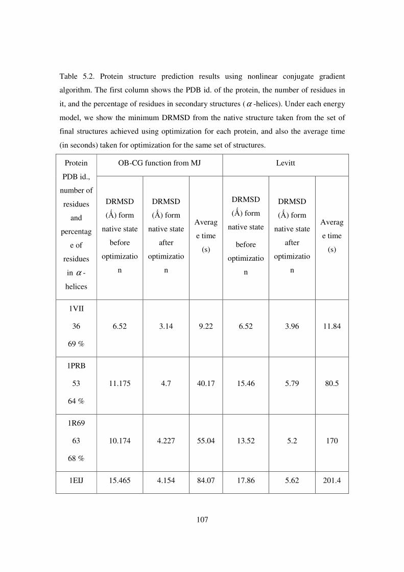
107

Table 5.2. Protein structure prediction results using nonlinear conjugate gradient

algorithm. The first column shows the PDB id. of the protein, the number of residues in

it, and the percentage of residues in secondary structures (α -helices). Under each energy

model, we show the minimum DRMSD from the native structure taken from the set of

final structures achieved using optimization for each protein, and also the average time

(in seconds) taken for optimization for the same set of structures.

OB-CG function from MJ Levitt Protein

PDB id.,

number of

residues

and

percentag

e of

residues

in α -

helices

DRMSD

(Ǻ) form

native state

before

optimizatio

n

DRMSD

(Ǻ) form

native state

after

optimizatio

n

Averag

e time

(s)

DRMSD

(Ǻ) form

native state

before

optimizatio

n

DRMSD

(Ǻ) form

native state

after

optimizatio

n

Averag

e time

(s)

1VII

36

69 %

6.52 3.14 9.22 6.52 3.96 11.84

1PRB

53

64 %

11.175 4.7 40.17 15.46 5.79 80.5

1R69

63

68 %

10.174 4.227 55.04 13.52 5.2 170

1EIJ 15.465 4.154 84.07 17.86 5.62 201.4

108

72

68 %

1LRE

81

74 %

14.79 3.886 68.17 17.4 6.05 237.8

1BCF

(chain A)

158

78 %

55.13 6.66 810.08 22.7 8.9 3599.6

1LYD

164

65 %

29.8 8.65 288.24 22.9 9.9 1926.6

using both energy models. Here, we only show the minimum DRMSDs that we get for

each protein from the set of different initial structures. To convey to the reader a sense of

the unfoldedness of the structures that we use as initial inputs (which are not shown

using three-dimensional figures or contact maps), we also show the DRMSD of the

corresponding initial structures for all proteins for both energy models. One can note

from Table 5.2 that gradient-based optimization methods are able to achieve a two to

four-fold reduction in DRMSD from the native structure. We also show the average time

(in seconds) taken for optimization of each protein structure for both the energy models

using the nonlinear conjugate algorithm.

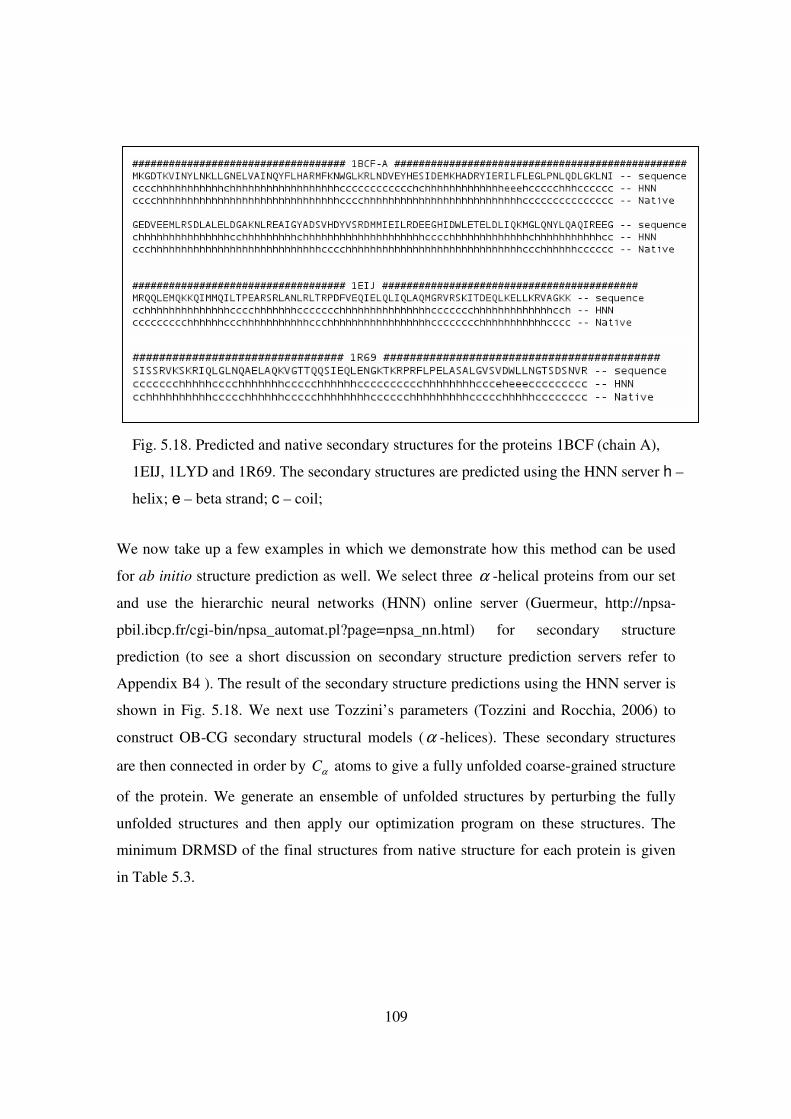
109

We now take up a few examples in which we demonstrate how this method can be used

for ab initio structure prediction as well. We select three α -helical proteins from our set

and use the hierarchic neural networks (HNN) online server (Guermeur, http://npsa-

pbil.ibcp.fr/cgi-bin/npsa_automat.pl?page=npsa_nn.html) for secondary structure

prediction (to see a short discussion on secondary structure prediction servers refer to

Appendix B4 ). The result of the secondary structure predictions using the HNN server is

shown in Fig. 5.18. We next use Tozzini’s parameters (Tozzini and Rocchia, 2006) to

construct OB-CG secondary structural models (α -helices). These secondary structures

are then connected in order by Cα atoms to give a fully unfolded coarse-grained structure

of the protein. We generate an ensemble of unfolded structures by perturbing the fully

unfolded structures and then apply our optimization program on these structures. The

minimum DRMSD of the final structures from native structure for each protein is given

in Table 5.3.

Fig. 5.18. Predicted and native secondary structures for the proteins 1BCF (chain A),

1EIJ, 1LYD and 1R69. The secondary structures are predicted using the HNN server h –

helix; e – beta strand; c – coil;

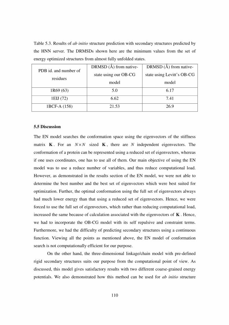
110

Table 5.3. Results of ab initio structure prediction with secondary structures predicted by

the HNN server. The DRMSDs shown here are the minimum values from the set of

energy optimized structures from almost fully unfolded states.

PDB id. and number of

residues

DRMSD (Ǻ) from native-

state using our OB-CG

model

DRMSD (Ǻ) from native-

state using Levitt’s OB-CG

model

1R69 (63) 5.0 6.17

1EIJ (72) 6.62 7.41

1BCF-A (158) 21.53 26.9

5.5 Discussion

The EN model searches the conformation space using the eigenvectors of the stiffness

matrix K . For an N N× sized K , there are N independent eigenvectors. The

conformation of a protein can be represented using a reduced set of eigenvectors, whereas

if one uses coordinates, one has to use all of them. Our main objective of using the EN

model was to use a reduce number of variables, and thus reduce computational load.

However, as demonstrated in the results section of the EN model, we were not able to

determine the best number and the best set of eigenvectors which were best suited for

optimization. Further, the optimal conformation using the full set of eigenvectors always

had much lower energy than that using a reduced set of eigenvectors. Hence, we were

forced to use the full set of eigenvectors, which rather than reducing computational load,

increased the same because of calculation associated with the eigenvectors of K . Hence,

we had to incorporate the OB-CG model with its self repulsive and constraint terms.

Furthermore, we had the difficulty of predicting secondary structures using a continuous

function. Viewing all the points as mentioned above, the EN model of conformation

search is not computationally efficient for our purpose.

On the other hand, the three-dimensional linkage/chain model with pre-defined

rigid secondary structures suits our purpose from the computational point of view. As

discussed, this model gives satisfactory results with two different coarse-grained energy

potentials. We also demonstrated how this method can be used for ab initio structure

111

prediction starting from the sequence with the aid of secondary structure prediction

servers. Henceforth, in our simultaneous sequence and conformation search problem, we

use this strategy of structure prediction from a sequence.

5.6 Closure

In this chapter, we described the formulation of our coarse-grained energy potential based

on the MJ matrix and two methods of searching the conformation space. We also

described the formulation of a continuous function, which when optimized, gives coarse-

grained model of alpha helices starting from a fully unfolded state of polypeptides. Both

the conformation search methods are validated for structure prediction by considering

proteins of different chain sizes. Based on the performance of these methods, we selected

a method for using in the simultaneous search of the sequence and conformation spaces.

112

6. Simultaneous search in the sequence and

conformation spaces: an application

• We consider the re-design of an existing enzyme as a demonstration of our

simultaneous sequence and conformation search strategy.

• A brief description of the target protein, the hen egg-white lysozyme, is given.

• We describe the modeling of the target protein and present the results.

• We discuss the computational methods and the simultaneous sequence and

conformation search strategy in the light of the results.

• The chapter is concluded with a summary.

6.1 Introduction

In this chapter, we present an application of the sequence and conformation search

techniques that are presented in the last two chapters. We combine these methods to

develop a step-by-step procedure for simultaneous sequence and conformation search for

computational protein design as mentioned in the problem statement section of the first

chapter. We take up the computational re-design of an actual protein, the hen-egg white

lysozyme (PDB ID 1LZE). The re-design of an existing protein was taken up because of

lack of access to experimental knowledge and facilities to design an actual protein that

can be experimentally validated. As mentioned in the introduction chapter, the goal of

our work is to give a method of protein design with structural and functional

specifications using gradient-based continuous optimization techniques. The structural

and functional specifications can be posed as constraints in the optimization problem.

Thus, if a few amino acids are crucial for a specific function of the target protein, those

type of amino acids are fixed in the corresponding positions in the sequence while we

search the sequence space for minimum-energy sequences. Again, if a part of the

conformation is important for the function of the target protein, for example, a ligand or

substrate-binding site, that part of the protein conformation can be modeled as a rigid

structure while we search the conformation space for minimum-energy conformations.

The aim of combining the sequence and conformation search techniques is that when

used iteratively, we should achieve convergence both in sequence and conformation

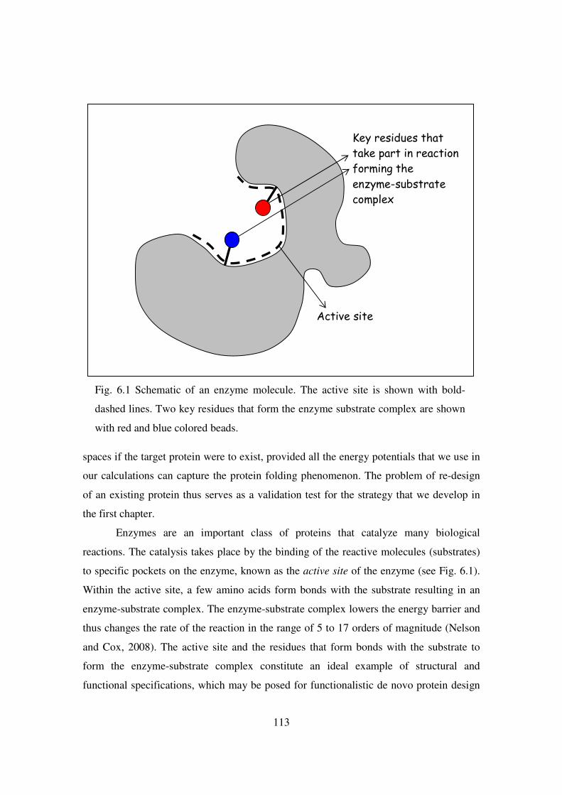
113

spaces if the target protein were to exist, provided all the energy potentials that we use in

our calculations can capture the protein folding phenomenon. The problem of re-design

of an existing protein thus serves as a validation test for the strategy that we develop in

the first chapter.

Enzymes are an important class of proteins that catalyze many biological

reactions. The catalysis takes place by the binding of the reactive molecules (substrates)

to specific pockets on the enzyme, known as the active site of the enzyme (see Fig. 6.1).

Within the active site, a few amino acids form bonds with the substrate resulting in an

enzyme-substrate complex. The enzyme-substrate complex lowers the energy barrier and

thus changes the rate of the reaction in the range of 5 to 17 orders of magnitude (Nelson

and Cox, 2008). The active site and the residues that form bonds with the substrate to

form the enzyme-substrate complex constitute an ideal example of structural and

functional specifications, which may be posed for functionalistic de novo protein design

Active site

Key residues that

take part in reaction

forming the

enzyme-substrate

complex

Fig. 6.1 Schematic of an enzyme molecule. The active site is shown with bold-

dashed lines. Two key residues that form the enzyme substrate complex are shown

with red and blue colored beads.

114

problem. This motivates us to consider the re-design of an enzyme, namely, the hen egg-

white lysozyme (PDB ID 1LZE), as an application of our computational protein design

strategy.

Before embarking on the application of our simultaneous sequence and

conformation search method and presentation of the results that we have achieved, we

would like to convey to the reader the broad perspective with respect to which this work

should be judged. As mentioned in the introductory chapter, developing computational

methods for functionalistic de novo protein design is a challenging problem (Baker,

2010). The difficulty of the problem can be understood when one realizes that both ab

initio structure prediction and de novo sequence design, the key constituents of

functionalistic de novo protein design (Schueler-Furman, 2005), are open problems by

themselves, and any generalized computational method for both these problems has not

yet been developed. Furthermore, each technique, when combined with the other, result

in issues for which the corresponding techniques were not developed individually. For

example, generating sequences and rotamer libraries for flexible backbone templates, and

ab initio structure prediction for large libraries of designed sequences, may encounter

problems when they are used in conjunction with other techniques. The best performing

methods for one problem (e.g., de novo sequence design) when used to address the larger

problem (i.e., simultaneous search of sequence and conformation spaces) results in a

computational deadlock. For instance, using the DEE method for de novo sequence

design for flexible backbone templates is computationally intractable. Thus, one of the

ways of approaching the larger problem will be to use models and techniques which may

give less accurate results but are computationally affordable. The work done in this thesis

takes this approach.

We have developed computational models and methods which are

computationally efficient and can be implemented on desktop computers, but, the

computational efficiency comes at the cost of accuracy. Each of these methods, i.e.,

sequence and conformation search techniques, were tested individually by considering

several examples. Now, we combine these methods; the results are a combination of the

pros and cons inherent in the methods and models that we use. We would further like to

point to the reader that the aim of this thesis is not the computational re-design of the hen

115

egg-white lysozyme (PDB ID 1LZE). The hen egg-white lysozyme is a good textbook

example of an enzyme whose activity and structural details are well understood (Nelson

and Cox, 2008). Furthermore, because of certain structural details which appear to be

conducive to our method (we discuss these details in the relevant section on modeling),

we consider it as an example of the application of the sequence and conformation search

techniques that we have developed. However, there are certain structural details of 1LZE

that have not been accounted for in our model; for example, pairing of Cystine residues to

form disulphide bonds. Thus, this example of application of our technique should be

judged more from the generalized computational point of view and less from the

convergence of results towards the particular protein taken up as a demonstrative

example.

6.2 A brief description of the target protein: The hen egg-white Lysozyme

The hen-egg white lysozyme (PDB ID 1LZE) is a 129 residue enzyme (see Fig. 6.2a) that

cleaves the carbohydrate peptidoglycan found in the cell walls of many bacteria (Nelson

and Cox, 2008). This protein was the first among enzymes to have its three-dimensional

structure determined by David Phillips and colleagues in 1965. There are four disulphide

bonds between Cystine pairs at the following positions: 6-127, 30-115, 64-80 and 76-94

(Maenaka et al., 1995). The key catalytic amino acid residues are Glu35 and Asp52 which

form intermediate bonds with the C—O bond between the N-acetylmuramic (Mur2Ac,

also referred as NAM) and the N-acetylglucosamine (GlcNAc, also referred as NAG)

sugar residues in the peptidoglycan molecule, ultimately leading to the cleavage of the

abovementioned C—O bond. Two different reaction pathways elucidating the enzymatic

action of this lysozyme have been proposed, the SN1 (Phillips mechanism) and the SN2

pathways (Withers et al., 2001). The details of these pathways can be found in relevant

texts (Nelson and Cox, 2008). At present, the SN2 pathway is more in agreement with

experimental results (Nelson and Cox, 2008). The sequence and the secondary structures

of 1LZE are shown in Fig. 6.2b.

116

Fig. 6.2a. A ribbon diagram of the hen egg-white lysozyme (PDB ID 1LZE). The

key catalytic residues, namely, Glu35 and Asp52 are shown as ball and stick models.

The portion of the structure which is assumed to have a fixed conformation is

colored blue.

b. The wild-type sequence of the hen egg-white lysozyme (PDB ID 1LZE). The

secondary structures are shown below the sequence: h – Alpha helix; e – Beta

strand.

Asp52

Glu35

(a)

(b)

117

6.3 Modeling and results

We follow the step-by-step design procedure for computational re-design of 1LZE as

outlined in Fig. 1.7 and in the problem statement section of the introduction chapter. The

problem statement requires that a few residues and a part of the conformation be

specified as inputs to the problem. In the case of 1LZE, we take Glu35 and Asp52 as the

specified residues which are fixed at 35th and 52nd positions respectively in the sequence

while designing the same. For the other specified quantity, i.e., a part of the

conformation, we chose the part of the conformation occupied by residues numbering

from 42 to 60. This is that part of the conformation where a β -sheet is formed from

pairing of three β -strands (shown in blue color in Fig. 6.2a). Although this part of the

conformation is spatially situated close to the active site and may play a role in the

stabilization of the same, we admit that we chose this part because our tertiary structure

prediction program cannot predict pairing of β -strands to form β -sheet. Thus, the

choice of the part of the conformation occupied by residue numbers 42-60 was more

guided by computational considerations than by biological significance. Here, we would

also like to point out that one of the reasons of selecting 1LZE as the target protein is

because of dominance of α -helices among its secondary structures (Fig. 6.2 b).

At present, our design method can consider only single-chain proteins. Thus,

before starting design, we consider the single chain information of 1LZE as a given

information. Furthermore, since this design strategy works for a fixed number of design

variables, the number of residues in the protein, i.e., 129, is also assumed to be a

specified quantity. Hence, the following are the inputs to the re-design of 1LZE:

i. the number of chains: 1.

ii. the number of residues: 129.

iii. fixed residues: Glutamic acid and Aspartic acid at positions 35 and 52

respectively.

iv. fixed conformation: The Cα coordinates from residue numbers 42-60.

v. apart from the fixed conformation the target protein comprises predominantly α -

helices, and

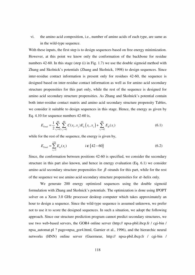
118

vi. the amino acid composition, i.e., number of amino acids of each type, are same as

in the wild-type sequence.

With these inputs, the first step is to design sequences based on free energy minimization.

However, at this point we know only the conformation of the backbone for residue

numbers 42-60. In this stage (step (i) in Fig. 1.7) we use the double sigmoid method with

Zhang and Skolnick’s potentials (Zhang and Skolnick, 1998) to design sequences. Since

inter-residue contact information is present only for residues 42-60, the sequence is

designed based on inter-residue contact information as well as for amino acid secondary

structure propensities for this part only, while the rest of the sequence is designed for

amino acid secondary structure propensities. As Zhang and Skolnick’s potential contain

both inter-residue contact matrix and amino acid secondary structure propensity Tables,

we consider it suitable to design sequences in this stage. Hence, the energy as given by

Eq. 4.10 for sequence numbers 42-60 is,

( )60 60 60

42 42 42

1( , ) , ( )

2i j i

Total i j ij i j i

x x x

E C x x E x x E xβ= = =

= +∑ ∑ ∑ (6.1)

while for the rest of the sequence, the energy is given by,

{ }129

1

( ) 42 60i

Total i

x

E E x iα=

= ∉ −∑ (6.2)

Since, the conformation between positions 42-60 is specified, we consider the secondary

structure in this part also known, and hence in energy evaluation (Eq. 6.1) we consider

amino acid secondary structure propensities for β -strands for this part, while for the rest

of the sequence we use amino acid secondary structure propensities for α -helix only.

We generate 200 energy optimized sequences using the double sigmoid

formulation with Zhang and Skolnick’s potentials. The optimization is done using IPOPT

solver on a Xeon 3.0 GHz processor desktop computer which takes approximately an

hour to design a sequence. Since the wild-type sequence is assumed unknown, we prefer

not to use it to score the designed sequences. In such a situation, we adopt the following

approach. Since our structure prediction program cannot predict secondary structures, we

use two web-based servers, the GOR4 online server (http:// npsa-pbil.ibcp.fr / cgi-bin /

npsa_automat.pl ? page=npsa_gor4.html, Garnier et al., 1996), and the hierarchic neural

networks (HNN) online server (Guermeur, http:// npsa-pbil.ibcp.fr / cgi-bin /

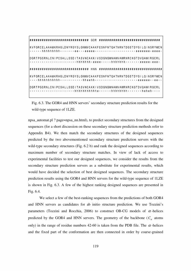
119

npsa_automat.pl ? page=npsa_nn.html), to predict secondary structures from the designed

sequences (for a short discussion on these secondary structure prediction methods refer to

Appendix B4). We then match the secondary structures of the designed sequences

predicted by the two abovementioned secondary structure prediction servers with the

wild-type secondary structures (Fig. 6.2 b) and rank the designed sequences according to

maximum number of secondary structure matches. In view of lack of access to

experimental facilities to test our designed sequences, we consider the results from the

secondary structure prediction servers as a substitute for experimental results, which

would have decided the selection of best designed sequences. The secondary structure

prediction results using the GOR4 and HNN servers for the wild-type sequence of 1LZE

is shown in Fig. 6.3. A few of the highest ranking designed sequences are presented in

Fig. 6.4.

We select a few of the best-ranking sequences from the predictions of both GOR4

and HNN servers as candidates for ab initio structure prediction. We use Tozzini’s

parameters (Tozzini and Rocchia, 2006) to construct OB-CG models of α -helices

predicted by the GOR4 and HNN servers. The geometry of the backbone ( Cα atoms

only) in the range of residue numbers 42-60 is taken from the PDB file. The α -helices

and the fixed part of the conformation are then connected in order by coarse-grained

Fig. 6.3. The GOR4 and HNN servers’ secondary structure prediction results for the

wild-type sequence of 1LZE.

120

121

beads to construct an unfolded structure, which serves as initial input to the tertiary

structure prediction program. We consider first five to ten of the highest-ranking

sequences predicted by each server and generate an ensemble of unfolded conformations

in a manner similar to that described in the chapter 5. For each sequence, approximately

50-100 unfolded conformations are generated. Thus, we generate approximately 1000

conformations to search the conformation space. Next, we optimize these structures to

form an ensemble of energy optimized structures. Since, the number of conformations to

be optimized is quite large (approximately 1000 in number), we use the nonlinear

conjugate gradient method which uses the one-bead coarse-grained (OB-CG) model with

rigid secondary structures. We use both the coarse-grained energy potentials, i.e., our

continuous function formulation incorporating the MJ matrix (Eq. 5.1) and Levitt’s

potentials (Eqs. 5.7 and 5.8) to predict tertiary structures from the abovementioned

unfolded states. We show two such predicted structures in Fig. 6.5 (b and d). The

unfolded states from which these structures were achieved are also shown (Fig. 6.5 a and

c respectively). A few of the best optimized structures are presented in Table 6.1. The

average time taken for optimization using nonlinear conjugate gradient on a Xeon 3.0

GHz processor desktop computer with Levitt’s model is approximately one hour, whereas

for our continuous function formulation incorporating the MJ matrix it is approximately

6-10 minutes.

In Table 6.1, we show the results of both the energy models. Under each energy

model, the first column indicates the DRMSD of the unfolded structures from the native

conformation in the PDB file 1LZE. The second column indicates the DRMSD of the

conformation after optimization using the corresponding potentials. In Table 6.1, we use

Fig. 6.4. Few of the designed sequences having high secondary structure prediction

similarity with wild-type secondary structure of 1LZE. The corresponding server

name, i.e., either GOR or HNN is indicated at the top before the sequences and

corresponding secondary structure prediction results are shown. The number of

secondary structure matches are also indicated. The secondary structures are

indicated below the sequences. As before, h – alpha helix and e – beta strand.

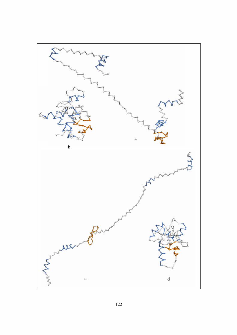
122

a

b

c d

123

a second metric apart from DRMSD, namely, the Template Modeling (TM) score (Zhang

and Skolnick, 2004, 2005). The TM-score is independent of the size of the protein and

can identify protein substructures (Zhang and Skolnick, 2004). Furthermore, recently it

has been claimed that the TM-score can be used for protein topology classification, i.e.,

“protein pairs with a TM-score >0.5 are mostly in the same fold while those with a TM-

score <0.5 are mainly not in the same fold” (Xu and Zhang, 2010). Thus, in the absence

of experimental verifications, the TM-score, apart from the DRMSD, can be considered

to be a suitable metric to rank our predicted tertiary structures. As shown in Table 6.1, we

achieved the highest TM-scores of 0.456 using Levitt’s potentials and 0.36 using our OB-

CG function from MJ matrix. The corresponding conformations are shown in figs. 6.5 b

and 6.5 d respectively. We consider the conformation shown in Fig. 6.4b as the best

conformation among all predicted conformations. This completes Step (iv) in our

simultaneous sequence and conformation search flow-diagram (Fig. 1.7).

In the next step, we design energy minimized sequences and further test them for

stability. Since, the tertiary structure is now available, we use the quadratic programming

method with atomistic potentials and amino acid composition constraints. Thus, in this

step we use the optimization function given by Eqs. 4.14 and 4.15. We generate Table

Fig.6.5. Tertiary structure prediction results using OB-CG model and rigid

secondary structures. The alpha-helices are colored blue; the part of the

conformation which we consider fixed, i.,e., backbone for residues 42-60 is colored

orange. The initial inputs to optimization are the conformations (a) and (c). The

final conformations after optimization are (b) and (c) respectively.

a) Initial conformation to optimization. The DRMSD from native state of 1LZE is

41.5 Å.

b) Final conformation after optimization from the structure shown in (a). The

DRMSD from native state of 1LZE is 7.52 Å.

c) Initial conformation to optimization. The DRMSD from native state of 1LZE is

46.2 Å.

d) Final conformation after optimization from the structure shown in (c). The

DRMSD from native state of 1LZE is 8.32 Å.

124

6.1. Few selected examples of tertiary structure prediction results using both energy

models. Under each energy model, the first column indicates the DRMSD of the unfolded

conformation from 1LZE ( C α− coordinates only) which serves as input to optimization

program. The second column is the DRMSD of the energy optimized structure from

1LZE ( C α− coordinates only). The third column shows the TM-score of the same

energy optimized structure. The conformation of the two highest TM-scoring structures

(0.456 and 0.36) are shown in figs. 6.4.b and 6.4.d respectively. The unfolded structures

from which these structures were achieved are shown in figs. 6.4.a and 6.4.c respectively.

OB-CG function from MJ Levitt

DRMSD

(Ǻ) form

native state

before

optimization

DRMSD

(Ǻ) form

native state

after

optimization

TM-score

DRMSD

(Ǻ) form

native state

before

optimization

DRMSD

(Ǻ) form

native state

after

optimization

TM-score

46.2 8.32 0.36 41.5 7.52 0.456

36.83 8.38 0.31 23.6 7.9 0.34

65.4 8.56 0.32 33.67 7.83 0.32

16.05 7.34 0.34 29.35 7.66 0.4

51.6 8.2 0.31 24.9 8.04 0.32

44.2 8.34 0.304 23.7 8.68 0.35

approximately 200 energy minimized sequences using the quadratic programming

method. The average time taken for designing each sequence by the IPOPT optimization

solver on a Xeon 3.0 GHz computer was approximately 10-12 hours. As mentioned

before, (step (vi) in Fig. 1.7), our aim now is to select the best sequence among these

designed sequences based on specificity requirements, i.e., the sequence which shows

maximum energy gap and minimum energy dispersion with respect to the selected

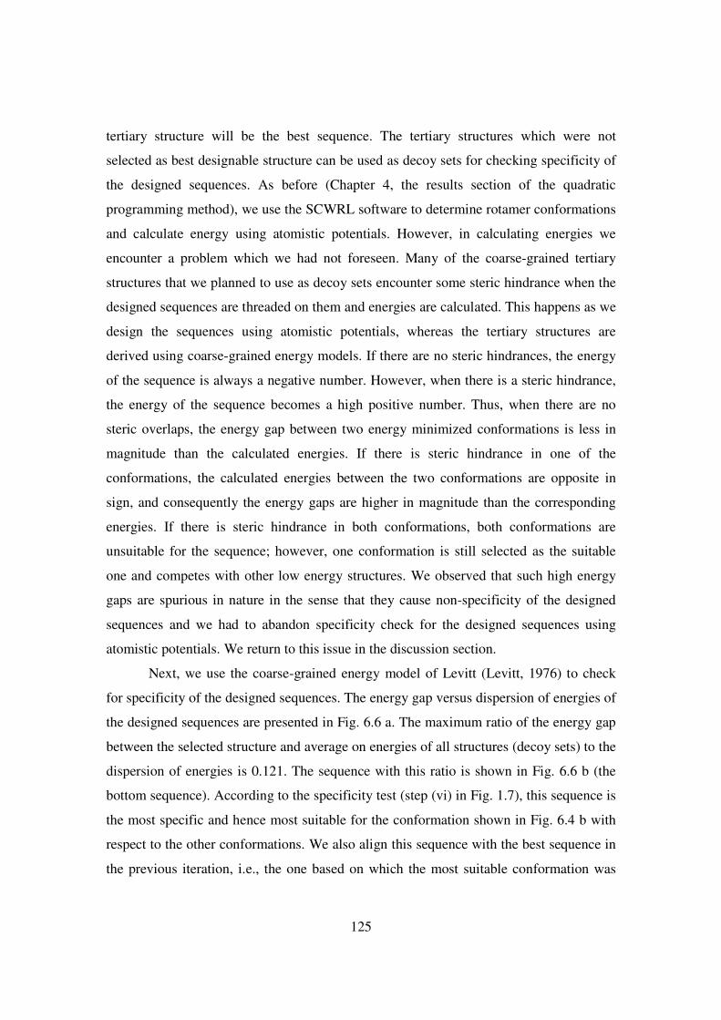
125

tertiary structure will be the best sequence. The tertiary structures which were not

selected as best designable structure can be used as decoy sets for checking specificity of

the designed sequences. As before (Chapter 4, the results section of the quadratic

programming method), we use the SCWRL software to determine rotamer conformations

and calculate energy using atomistic potentials. However, in calculating energies we

encounter a problem which we had not foreseen. Many of the coarse-grained tertiary

structures that we planned to use as decoy sets encounter some steric hindrance when the

designed sequences are threaded on them and energies are calculated. This happens as we

design the sequences using atomistic potentials, whereas the tertiary structures are

derived using coarse-grained energy models. If there are no steric hindrances, the energy

of the sequence is always a negative number. However, when there is a steric hindrance,

the energy of the sequence becomes a high positive number. Thus, when there are no

steric overlaps, the energy gap between two energy minimized conformations is less in

magnitude than the calculated energies. If there is steric hindrance in one of the

conformations, the calculated energies between the two conformations are opposite in

sign, and consequently the energy gaps are higher in magnitude than the corresponding

energies. If there is steric hindrance in both conformations, both conformations are

unsuitable for the sequence; however, one conformation is still selected as the suitable

one and competes with other low energy structures. We observed that such high energy

gaps are spurious in nature in the sense that they cause non-specificity of the designed

sequences and we had to abandon specificity check for the designed sequences using

atomistic potentials. We return to this issue in the discussion section.

Next, we use the coarse-grained energy model of Levitt (Levitt, 1976) to check

for specificity of the designed sequences. The energy gap versus dispersion of energies of

the designed sequences are presented in Fig. 6.6 a. The maximum ratio of the energy gap

between the selected structure and average on energies of all structures (decoy sets) to the

dispersion of energies is 0.121. The sequence with this ratio is shown in Fig. 6.6 b (the

bottom sequence). According to the specificity test (step (vi) in Fig. 1.7), this sequence is

the most specific and hence most suitable for the conformation shown in Fig. 6.4 b with

respect to the other conformations. We also align this sequence with the best sequence in

the previous iteration, i.e., the one based on which the most suitable conformation was

126

Fig. 6.6. a) Plots of energy gap (E target structure avg decoys

E E− −∆ = − ) versus Eσ (the

standard deviation of energy of the decoy set structures) for the designed sequences.

The target structure is the conformation shown in Fig. 6.4 b. The sequence that has

maximum /E Eσ∆ ratio is shown on the plot with the red dot.

b) The sequence with maximum /E Eσ∆ (bottom one) aligned with the best

designed sequence in the previous iteration (top one), i.e., the sequence for the

conformation in Fig. 6.4 b, using CLUSTAL (version 1.83) software.

(a)

(b)

127

achieved (Fig. 6.5 b). The determination of this sequence completes one iteration of our

simultaneous sequence and conformation search method (flowchart presented in Fig.

1.7).

6.4 Discussion

In the last section we presented one iteration in the loop of the flowchart of simultaneous

sequence and conformation search presented in Fig. 1.7. Before proceeding further, i.e.,

going through the second loop in the iteration which may take more than one month even

after our stress on computationally efficient techniques, one needs to re-evaluate the

computational techniques in the light of the results presented in the previous section. In

this section we evaluate the computational techniques and models in the order in which

the results were presented in the previous section. However, we do not question the

specified conditions, for example, how does one know beforehand the number of residues

or chains or the amino acid composition of the protein which is to be designed, which our

simultaneous sequence and conformation search technique requires as minimum inputs.

In the first stage we designed sequences using the double sigmoid method and

Zhang and Skolnick’s potentials. Although, the use of statistical potentials has been

questioned in designing sequences (Thomas and Dill, 1996), and methods have been

suggested for deriving statistical potentials based on the target backbone and decoy sets

(Mirny and Shakhnovich, 1996), we consider the use of Zhang and Skolnick’s potentials

in the first step justified, as minimal information is available at this stage in our problem,

viz. the length of the sequence and the backbone conformation for a limited part of the

chain. We had to consider a potential which does not depend on the tertiary structure

information, and a potential based on secondary structure propensities best suits this

purpose. However, once the sequences are designed, we do not rank them according to

energy, but with respect to some other criteria (like energy gap and energy dispersion).

Again, since no information on conformation for the whole sequence or decoy structures

is available, we could not apply the method of ranking the sequences as in Chapter 4.

Instead, we decided to rank the sequences in the order of predicted secondary structure

matches with the wild-type sequence. To this end, we used two online secondary

structure prediction servers, and considered the results from them as substitute to

128

experimental data. However, as Fig. 6.3 shows, the secondary structure prediction results

from these two servers differs from actual secondary structures of 1LZE even for the

wild-type sequence. Thus the deviations incurred in misprediction of secondary structures

will affect tertiary structure prediction, which in turn will affect sequence prediction in

the next round, and this effect will go on increasing. To the best of our knowledge we do

not know any secondary structure prediction technique that is 100% accurate, and at this

point, we are not certain how this will affect the convergence of results in the sequence

and conformation spaces.

In the second stage, we predicted tertiary structures from unfolded conformations

with rigid secondary structures. The underlying assumption of this prediction is that

secondary structures are formed before tertiary structures. However, as modern theories

suggest (Sinha and Udgaonkar, 2009), the secondary and tertiary structures evolve

simultaneously and the formation of one effects the other and vice-versa. Thus, in the

ideal case we should do structure prediction in one step, rather than in two steps.

However, even though we tried to develop models to predict secondary structures based

on continuous optimization techniques (which is presented as a short section in Chapter

5), a continuous function that can simultaneously develop secondary and tertiary

structures when minimized is yet to be developed. Furthermore, the coarse-grained

energy potentials based on which we do tertiary structure prediction, namely the MJ

matrix and Levitt’s potentials have their own limitations in reflecting the actual energy

governing protein folding. The limitations of theses coarse-grained energy models

became apparent when we threaded designed sequences on the energy minimized

structures and tried to calculate energy based on atomistic potentials. Many of the

conformations, which occupy a minimum energy position in the energy-conformation

space encountered steric hindrances and consequently high energy when different

sequences were threaded onto them. The reason for this may be that, coarse-grained

potentials, being lower degree polynomials than their atomistic counterparts, allow the

residues to be packed together closer than is actually possible, and the extent of packing

grows with the size of the protein. In such a situation, we think the best remedy is to run

some fine-grained atomistic potential-based simulation such as molecular dynamics on

129

each of the tertiary structures derived using coarse-grained potentials. But that would

involve substantial computation power and time.

As an alternative, we tried the other option; we threaded the sequences and calculated

energy using coarse-grained potentials. The reader may question the test for specificity

using coarse-grained energy where the sequences were designed using atomistic

potentials. We agree that such a question is justified. However, as indicated in the

motivation section of Chapter 1, there are few examples of protein design using search in

both sequence and conformation spaces. We were motivated to find out whether the

question of convergence in sequence and conformation spaces can be asked at all with the

methods that we have developed. Thus, although we have used different potentials to

design sequence and check for specificity, all the blue colored dots in Fig. 6.6(a) indicate

that our simultaneous sequence and conformation search strategy indeed yield sequences

that show specificity of the designed target tertiary structure over other competitive

structures, even though marginally. Thus, the aim that we set to achieve is a feasible one

and methods that we developed show some promise.

6.5 Closure

In this chapter, we considered the re-design of an existing enzyme, the hen egg-white

lysozyme (PDB ID 1LZE) using the sequence design and conformation search tools that

we develop in the previous chapters. We briefly described the target protein and how we

model the re-design of the same protein. We next applied the simultaneous sequence and

conformation search strategy that we proposed in Chapter 1 and presented the results in a

stepwise manner as described in our method. We closed this chapter with a discussion on

the efficacy of the computational tools in the light of the results.

130

7. Towards parallelization of tertiary structure

prediction using Graphics Processor Unit (GPU)

based parallel computation

• We give a brief introduction and our motivation for GPU-based code for tertiary

structure prediction.

• We describe the logic of conversion of the CPU-based code to the GPU-based

code.

• We present a case study with CPU and GPU based codes and present the results.

• We close this chapter with a summary.

7.1 Introduction and motivation

In this chapter we describe our attempt to parallelize the tertiary structure prediction

computer program using Graphics Processor Unit (GPU) based parallel programming

computation model, the Compute Unified Device Architecture (CUDA) introduced by

NVIDIA in 2007 (Kirk and Hwu, 2010). We select the tertiary structure prediction

program over the sequence design program as the optimization solver (nonlinear

conjugate gradient) for tertiary structure prediction is coded in-house. The nature of the

tertiary structure prediction program further makes it suitable for parallel computation in

the following way.

The tertiary structure prediction program optimizes the free energy of the protein

molecule calculated as a function of the coordinates of the residues in the OB-CG model

(Eq. 5.4). Thus if there are N residues in a protein, there are ( )N○ variables. Here we

assume that after reducing the secondary structures as rigid bodies, there is no reduction

in the order of the number of optimization variables, which is the case for the proteins

considered in this work. While calculating the non-bonded interaction energies (Eq. 5.1

or 5.7), for every residue, its interaction energy with all other residues are calculated.

Thus, for the non-bonded interaction energy there are ( )2N○ calculations (one may

consider a reduced number of calculations based on a cut-off list of interacting residues,

but since there is large change in conformation during optimization, such a cut-off list

131

will have to be updated from time to time during optimization). Gradient-based

optimization requires the calculation of the gradient of the optimizing function with

respect to the design variables (Eq. 5.5) during every step in optimization. Thus, if the are

N variables in an optimization program, the gradient will contain N components that will

involve ( )N○ calculations. Hence, the gradient of the non-bonded interaction energy

will involve ( )3N○ calculations. Apart from the non-bonded energy, the bond length

and bond-angle constraints each individually involve ( )N○ calculations. Thus, their

gradients will individually involve ( )2N○ calculations. A typical example of tertiary

structure optimization presented in the last chapter involved 210 design variables and

8,128 non-bonded interactions. Thus, the gradient of the non-bonded energy will involve

8,128 210 1,706,880× = order of numerical calculations. Even though we coded our

tertiary structure prediction programs in C++ which is compiled using the Intel C++

compiler with O3 optimization options and employed on a 64 bit Xeon 3.0 GHz

computer with static memory allocation to minimize time for allocation and de-allocation

of memory, it still takes more than an hour on the average to run each simulation. The

main reason for this is that in the CPU based code, the large number of calculations

involved in calculating energies and their gradients are done sequentially through loops

(for or while), although each of these calculation is independent of one another (Fig.

7.1). Hence, much time can be saved if each of the energy calculations and the

corresponding gradients can be done in parallel. The ability of CUDA to handle large

number of numerical computations in parallel was the motive behind our effort to convert

the CPU based codes into GPU based codes.

Our GPU programs were run on a C1060 Tesla Cluster with CUDA driver

version 3.20. Our CPU programs were run on an Intel i7 2.67 GHz processor.

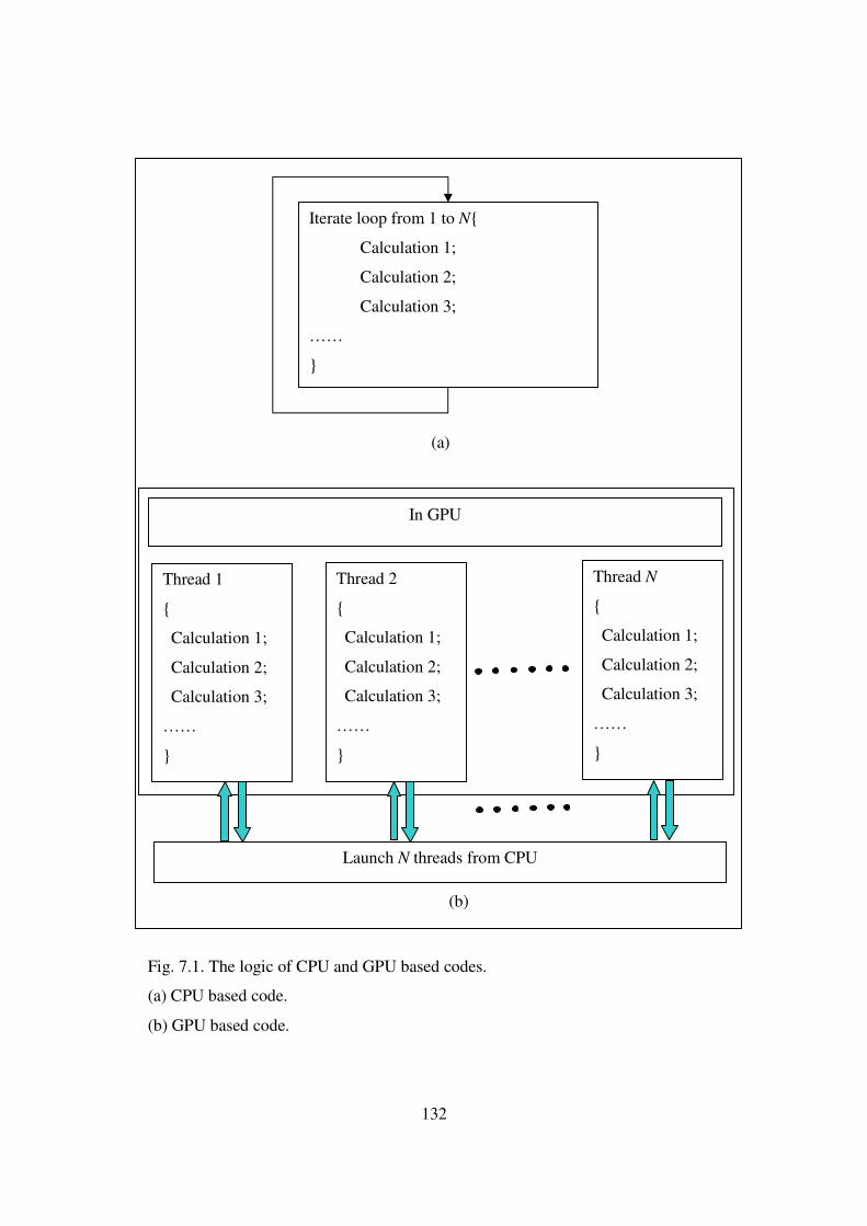
132

Iterate loop from 1 to N{

Calculation 1;

Calculation 2;

Calculation 3;

……

}

(a)

Fig. 7.1. The logic of CPU and GPU based codes.

(a) CPU based code.

(b) GPU based code.

Thread 1

{

Calculation 1;

Calculation 2;

Calculation 3;

……

}

Thread 2

{

Calculation 1;

Calculation 2;

Calculation 3;

……

}

Thread N

{

Calculation 1;

Calculation 2;

Calculation 3;

……

}

Launch N threads from CPU

In GPU

(b)

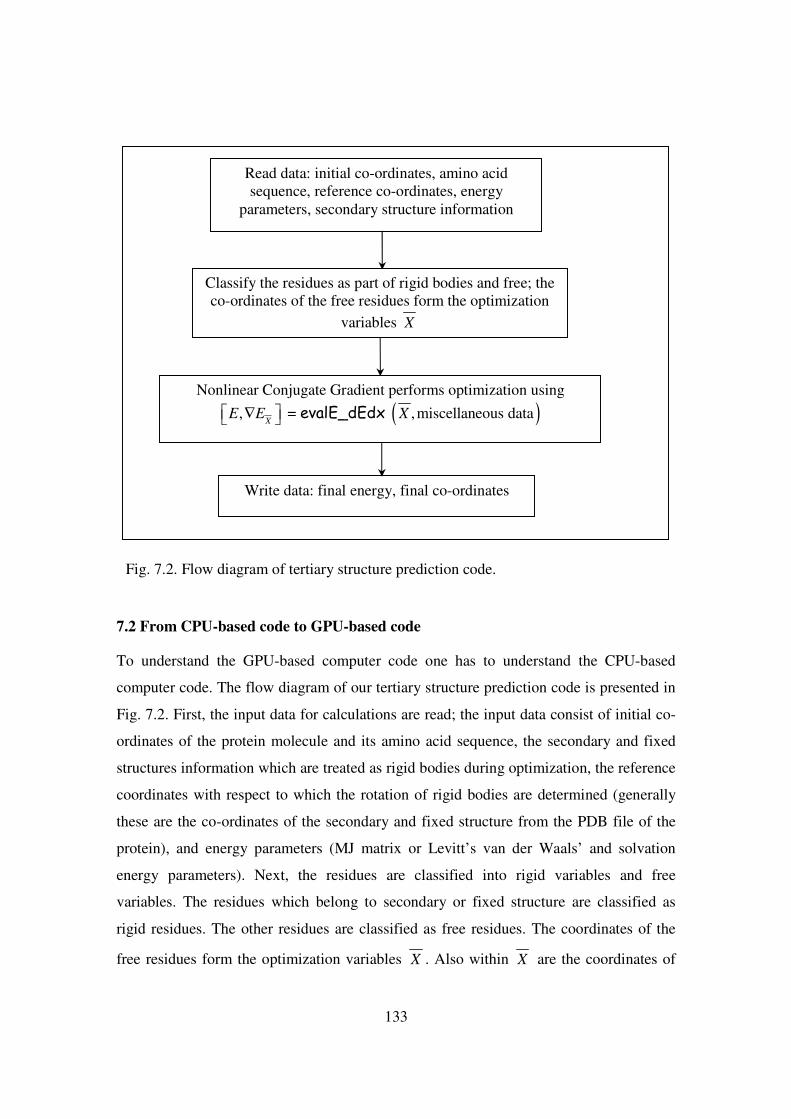
133

7.2 From CPU-based code to GPU-based code

To understand the GPU-based computer code one has to understand the CPU-based

computer code. The flow diagram of our tertiary structure prediction code is presented in

Fig. 7.2. First, the input data for calculations are read; the input data consist of initial co-

ordinates of the protein molecule and its amino acid sequence, the secondary and fixed

structures information which are treated as rigid bodies during optimization, the reference

coordinates with respect to which the rotation of rigid bodies are determined (generally

these are the co-ordinates of the secondary and fixed structure from the PDB file of the

protein), and energy parameters (MJ matrix or Levitt’s van der Waals’ and solvation

energy parameters). Next, the residues are classified into rigid variables and free

variables. The residues which belong to secondary or fixed structure are classified as

rigid residues. The other residues are classified as free residues. The coordinates of the

free residues form the optimization variables X . Also within X are the coordinates of

Fig. 7.2. Flow diagram of tertiary structure prediction code.

Read data: initial co-ordinates, amino acid sequence, reference co-ordinates, energy

parameters, secondary structure information

Write data: final energy, final co-ordinates

Nonlinear Conjugate Gradient performs optimization using

,X

E E ∇ = evalE_dEdx ( ),miscellaneous dataX

Classify the residues as part of rigid bodies and free; the co-ordinates of the free residues form the optimization

variables X

134

the first and last residues in a secondary structure which determines its position during

optimization and with respect to which the co-ordinates of the other residues inside that

secondary structure are calculated (Fig. 5.16). The optimization is done using the

nonlinear conjugate gradient algorithm which is presented in Appendix #. The nonlinear

conjugate gradient algorithm calls the function evalE_dEdx which calculates the bond

length (Eq. 5.3), the bond angle (Eq. 5.2) and the non-bonded (Eq. 5.1 or Eqs. 5.7 and

5.8) energies as functions of X and also the gradient of the same energies with respect to

X . As mentioned before, it is the calculation of the energies and their derivatives which

require maximum computational effort and is the target of parallelization; the other

functions, namely, reading data, classifying residues into free and rigid ones and

determining X , the nonlinear conjugate gradient, and writing functions are same for the

CPU and GPU-based codes, and is done on the CPU.

Let us now describe the function evalE_dEdx which is central to our

computation. The algorithm of evalE_dEdx is presented in Fig. 7.3. Each step in

evalE_dEdx can be done on the GPU. However, whenever a GPU based function is

called, some latency time is involved in transfer of data from CPU to GPU and back (ref.

CUDA manuals). If the number of calculations are small, then it is more efficient to do

the calculations on the CPU. Hence, a limit on the number of iterations for a specific

calculation which determines whether it will be done on the GPU or the CPU is

necessary; in our case, we choose this limit as 28 = 256. Thus, if the number of iterations

is less than 256, we do it on CPU; if greater, we do it on GPU. For the proteins on which

we have worked in this thesis, all the derivative calculations and non bondedE − fall in the

range of GPU, the rest are done on CPU. We next present the results for the GPU and

CPU based codes for a test case.

135

[ ,dE

Ed X

] = evalE_dEdx ( X , residueID, N , refX , RBdata, sequence, parametersE ){

1. Determine residue specific coordinates { }, ,x y z from design variable X

and derivatives of the same with respect to design variables.

( )1 if ( ) coordinate and ( ) variable represent the same coordinate

( )

in the same residue

0 otherwise

dx ix i X j

dX j=

=

2. Determine position of rigid bodies ( RBV ) by calculating the translation vector

transV and the rotation angle θ of RBV with respect to reference coordinates refX .

Calculate the rotation matrix ℜ for each rigid body. Calculate

, and transdV d d

d X d X d X

θ ℜ as follows,

{ } { }{ }

( )

( )

( )

11 2

2 11 2

2

1 2

( ) , , , ,

, ,( )

cos see Eq. 5.2

1

1

trans i i i ref ref ref

trans i i i

i

i i

RB

V i x y z x y z

d x y zdV i

d X d X

u u

dxd du duu u

dx dxd X d Xu u

d d d

dd X d X

V i V

θ

θ

θ

θ

−

= −

=

= •

−= • + •

− •

ℜ ℜ=

= ( )

( ) ( )

trans ref

RB trans

i V

dV i dV i d

d X d X d X

+ ℜ

ℜ= +

3. Calculate the position of the residues inside the rigid bodies using transV and ℜ .

Also, calculate their derivatives with respect to X .

4. Calculate bond length energy, bondedE (Eq. 5.3) and its derivatives with respect to

X , bondeddE

d X.

136

7.3 A case study with CPU and GPU based codes

We now consider an example for which we run both our CPU and GPU based codes and

see their performances. This example is an unfolded structure of hen egg-white lysozyme

(PDB ID 1LZE) with 129 residues in which the residue positions 42-60 are kept fixed

throughout optimization, i.e., they act like boundary conditions or constraints. There are

six secondary structures which are considered as rigid bodies during optimization. After

omitting the fixed part and considering the secondary structures as rigid bodies this

problem consist of 219 design variables. In Table 7.1 we show the time required by CPU

and GPU for different calculations in the algorithm of evalE_dEdx which is shown in

Fig. 7.3. In this table, we show results for those calculations for which the number of

iterations per function call of evalE_dEdx were greater than 256, for that is the limit

above which we do the calculation in the GPU as mentioned before.

(continued from previous page)

5. Calculate bond angle energy, Eθ (Eq. 5.2) and its derivatives with respect to X ,

dE

d X

θ .

6. Calculate nonbonded energy, (Eq. 5.1 or Eqs. 5.7 and 5.8) non bondedE − and its

derivatives with respect to X , non bondeddE

d X

− .

7. Calculate the total energy totalE (Eq. 5.4) and its derivatives totaldE

d X.

}

Fig. 7.3. Flowchart of the algorithm evalE_dEdx.

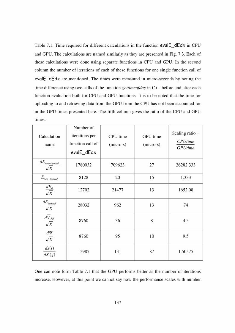
137

Table 7.1. Time required for different calculations in the function evalE_dEdx in CPU

and GPU. The calculations are named similarly as they are presented in Fig. 7.3. Each of

these calculations were done using separate functions in CPU and GPU. In the second

column the number of iterations of each of these functions for one single function call of

evalE_dEdx are mentioned. The times were measured in micro-seconds by noting the

time difference using two calls of the function gettimeofday in C++ before and after each

function evaluation both for CPU and GPU functions. It is to be noted that the time for

uploading to and retrieving data from the GPU from the CPU has not been accounted for

in the GPU times presented here. The fifth column gives the ratio of the CPU and GPU

times.

Calculation

name

Number of

iterations per

function call of

evalE_dEdx

CPU time

(micro-s)

GPU time

(micro-s)

Scaling ratio =

CPUtime

GPUtime

non bondeddE

d X

− 1780032 709623 27 26282.333

non bondedE − 8128 20 15 1.333

dE

d X

θ 12702 21477 13 1652.08

bondeddE

d X 28032 962 13 74

RBdV

d X 8760 36 8 4.5

d

d X

ℜ 8760 95 10 9.5

( )( )

dx i

dX j 15987 131 87 1.50575

One can note form Table 7.1 that the GPU performs better as the number of iterations

increase. However, at this point we cannot say how the performance scales with number

138

of iterations. It appears to depend on the nature of calculations. For example, both RBdV

d X

and d

d X

ℜ are iterated 8760 times; however, in the evaluation of

d

d X

ℜ the GPU is much

faster than the CPU than in the evaluation of RBdV

d X. There is another interesting point

which we would like to mention. It appears that the formula for all energy evaluation and

their derivatives pose complex tasks for the GPU. When we compiled with –arch=sm_13

option (required for double precision calculations) we got a failure message for all energy

and corresponding derivative function evaluations stating that memory and register

requirements were too high for all these functions. When we compiled with the

debugging option –g –G along with –arch=sm_13 option, the memory and register

requirements of these functions came down and we were able to run our program.

However, we are not sure as to how the –g –G option affects the performance of GPU2..

However, even with the –g –G option (about which we are not sure how it affects

the performance of the GPU) it leaves no doubt from the performance of the GPU as

presented in Table 7.1 that if we use the GPU based functions, the overall performance of

the optimization program (Fig. 7.2) will be much better. However, when we ran all our

inputs in the GPU based code, which amounts to a total of approximately 1000 initial

conformations, only in two cases the optimization code based on GPU actually converged

whereas, the optimization code based on CPU converges for greater than 99% cases. To

give the reader a feeling of how the CPU and GPU based codes converge to the final

result we present the results of iterations in Fig. 7.4. In this figure, we print the function

value and the norm of the gradient of the same for the function evalE_dEdx after every

219 (the number of variables in the chosen optimization problem) steps in optimization

using the nonlinear conjugate optimization program. Since the nonlinear conjugate

gradient algorithm consists of the linear conjugate gradient algorithm which is iterated

unless the function value or the gradient of the same converges, we chose the number of

2 Upon posting a message in the NVIDIA website as to why such a thing happens, the only reply received stated that our energy evaluation and derivative formulas were too complex to be handled in the GPU.

139

GPU code CPU code

continued on the next page…

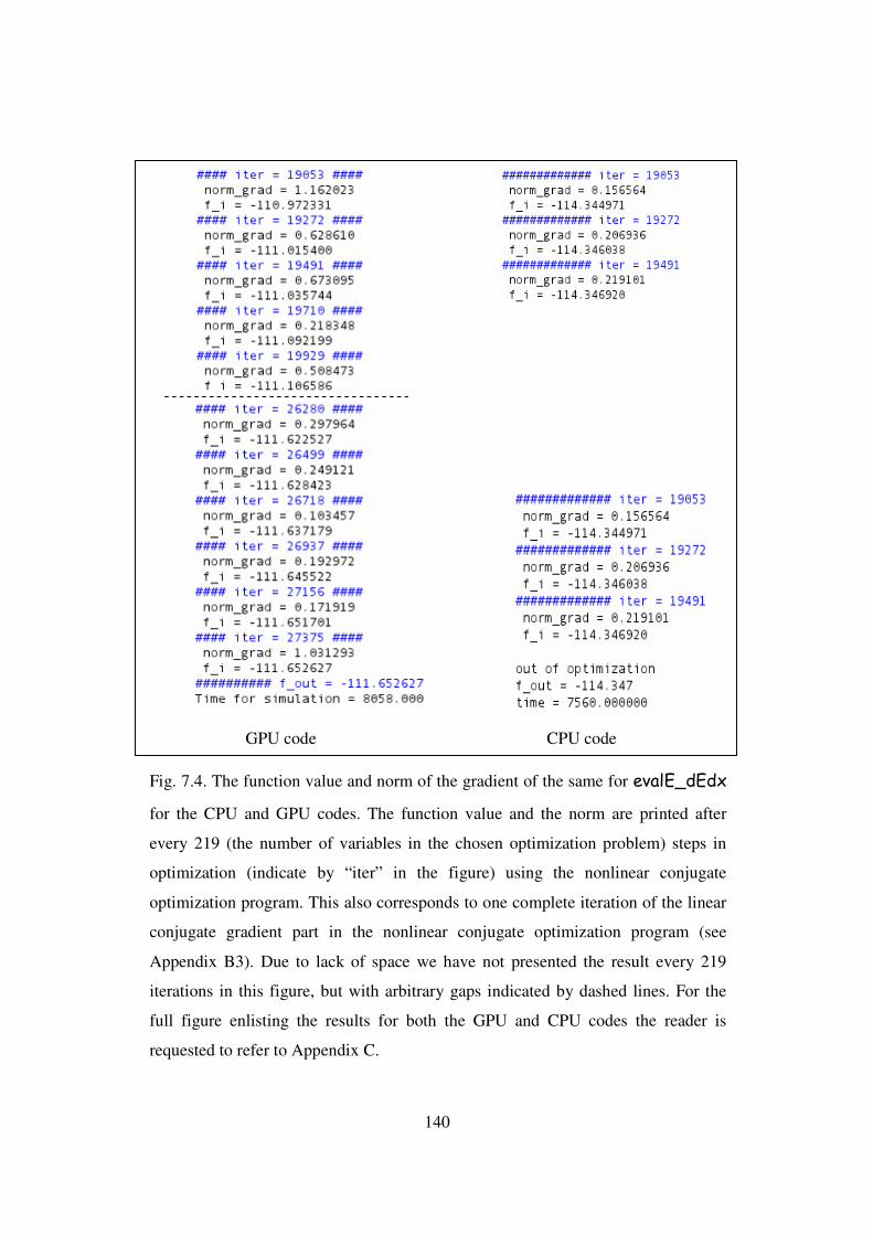
140

GPU code CPU code

Fig. 7.4. The function value and norm of the gradient of the same for evalE_dEdx

for the CPU and GPU codes. The function value and the norm are printed after

every 219 (the number of variables in the chosen optimization problem) steps in

optimization (indicate by “iter” in the figure) using the nonlinear conjugate

optimization program. This also corresponds to one complete iteration of the linear

conjugate gradient part in the nonlinear conjugate optimization program (see

Appendix B3). Due to lack of space we have not presented the result every 219

iterations in this figure, but with arbitrary gaps indicated by dashed lines. For the

full figure enlisting the results for both the GPU and CPU codes the reader is

requested to refer to Appendix C.

141

variables in optimization as a suitable step for printing values as it corresponds to the end

of every linear conjugate gradient solution to the nonlinear optimization problem. For a

comprehensive overview of the results, we do not present the full run in Fig. 7.4, but

insert gaps which are indicated with dashed lines in the same figure. The interested reader

is requested to refer to Appendix C for a step by step comparison of the performance of

the GPU and CPU codes.

We gave the same inputs and same set of energy calculation parameters to both

the CPU and GPU codes. At the start (iteration number 0), the results diverge by

55.41 10 %−× in function value and 54.4 10 %−× in the norm of the gradient, which we

ascribe due to the difference of the compilers, namely nvcc for the GPU code, and g++

for the CPU code. However, by 219 iterations we notice that the results for GPU and

CPU codes diverge by 2.41% in function evaluation and 10.75% in the norm of the

gradient. Towards the end, i.e., after 19272 iterations it appears that the GPU and CPU

codes have settled to their own, but slightly different converged values. However, we

notice that for a large number of iterations, i.e., from 19272 to 27375, i.e., for 8103 steps

the GPU code has run with small changes in the function value and oscillatory changes in

the gradient of the function which is indicated by its norm. This has lead to lower

performance of the GPU code which converged in 8058 s compared to the CPU code

which converged in 7560 s. We would also like to mention here that in the majority of

cases in which the GPU code failed (998 out of 100) as compared to the CPU code which

succeeded in 99% cases, the optimization in GPU showed such oscillatory nature of

gradient evaluations before failure in optimization. We did not investigate this matter any

further.

7.4 Closure

In this chapter we presented our efforts of parallelizing the tertiary structure prediction

program using GPU based CUDA programming model. We described our motivation for

going from CPU to GPU for tertiary structure prediction and present the logic of

converting the CPU-based code to the GPU-based code. We took up a test case and

present the times taken by various calculations in the CPU and the GPU. We also

presented the result of optimization for the GPU and CPU codes in steps so that their

performances can be compared.

142

8. Closure and Future Work

• The work presented in the thesis is summarized and its conclusions are noted.

• Contributions of this thesis are presented.

• Based on the conclusions, a few directions for future work are proposed.

8.1 Summary and Conclusions

The preceding chapters presented the computational methods that we developed and the

results that we achieved in our goal of functionalistic protein design using continuous

optimization methods. From our approach, it should be clear to the reader that wherever

possible, we have tried to formulate problems as continuous functions so that gradient-

based optimization techniques can be used. However, in a few instances (e.g., secondary

structure prediction) we have not been successful so far, and these problems can be taken

up as part of future work.

Protein design is an unsolved problem. Although questions have been raised in

the past on the feasibility of protein design, ingenious experiments have proved it to be

possible. However, theoretical models that can provide a sound basis for protein design

are yet to be developed. Even the atomistic potentials are questionable after a certain

limit of approximation, as they are not derived by solving Schrödinger’s wave equation,

as should be done in case of true atomistic potentials. So, the computational techniques

that are employed in protein design employ some form of knowledge-based parameters to

some extent or other, for example, from more or less generic atomistic potentials derived

from experimental results of small molecules to fully knowledge based statistical

potentials designed for specific proteins. Because of so much dependence on knowledge

derived from experiments over time, the computational techniques which are used for

protein design are almost always heuristic. However, we have tried to the best of our

efforts to adhere to computational methods that have a sound mathematical framework,

namely, gradient-based continuous optimization.

Computational protein design has sometimes been labeled as an N-P hard

problem, implying that it is intractable from theoretical and computational point of view.

Hence, we took a cautious approach when we set the goal of protein design and devised a

method of reducing the amino acid set from 20 to a much lower number for sequence

143

design. However, ultimately we did not use reduced amino acid sets in sequence design

as we came to learn and use IPOPT, a gradient-based optimization solver which can

handle nonlinear optimization problems with a large number of optimization variables

and nonlinear set of constraints. The sequences designed using IPOPT based on free

energy minimization were tested on two different uncorrelated design criteria different

from ours, namely, match with wild-type sequences and check for stability by calculating

the Z-score based on decoy sets. In the other domain of functionalistic protein design,

namely, structure prediction, we concentrated on coarse-grained models as fine grained

models can make the folding funnel of the designed protein rugged. With this view, we

developed our own continuous coarse-grained function from the Miyazawa-Jernigan inter

residue contact energy matrix. However, our efforts towards ab initio structure prediction

faced problems as the coarse-grained potentials developed were not conducive to

secondary structure formation. Keeping the larger goal of tertiary structure prediction

from sequence in view, we used web based servers for secondary structure prediction as

an intermediate step and went ahead with our own model of tertiary structure prediction

using continuous optimization. The tertiary structure prediction program was used with

two different coarse-grained energy models and validated on several proteins. We would

like to mention here that we have not been successful to formulate an optimization

function which can successfully pair up beta strands to form beta sheets which determine

the tertiary structure of proteins where beta sheets are present. The validations we

performed were only on alpha-helical proteins.

Once the tools were developed, we combined them to form a computational

strategy of simultaneous search in sequence and conformation spaces for functionalistic

protein design. The selection of a target protein was difficult as we have no resource of

experimental techniques or expertise. We chose the re-design of a well studied protein,

the hen egg-white lysozyme, which has a functionally active site and two key residues

that form the enzyme-substrate complex which can serve as the structural and functional

constraints in our optimization model. Although the tertiary structure of the hen egg-

white lysozyme is stabilized by four disulphide bonds and we had not taken into account

the formation of disulphide bonds in our optimization function formulation, we decided

to go ahead and see the structure prediction results with the tertiary structure prediction

144

program that we have developed. The structural constraint which we imposed was a part

of that part of the lysozyme structure dominated by beta sheets, and hence our selection

of that part was more guided by computational constraints than by actual functional

constraints of the same protein.

Following the simultaneous sequence and conformation search strategy proposed,

we first design sequences based on statistical potentials using only that part of the

structure specified as a functional constraint. At this point, a difficult situation arose

because of lack of access to experimental verification. The experimental results are much

needed feedback for rectifying computational models as the knowledgeable reader will

know. We could not also use the wild-type sequence as that would fail our purpose of re-

design of the hen egg-white lysozyme. One can argue that we could rank the designed

sequences in terms of their energy and select a small set possessing the lowest energies.

However, as our previous results on sequence design demonstrated a few limitations of

statistical potentials, we sought to devise a different criterion for selecting the designed

sequences based on maximum predicted secondary structure matches with the secondary

structures of lysozyme using web-based secondary structure prediction servers. With the

best ranked sequences selected as per the new design criterion, we did tertiary structure

prediction from approximately 1000 unfolded structures using two different coarse-

grained energy models and selected the structure with best TM-score. Following the

simultaneous sequence and conformation search strategy, we again designed sequences

for the selected tertiary structure, but now we used atomistic potentials and imposed

amino acid composition constraints to ensure stability of the designed sequences. This

time we test the designed sequences using the Z-score criterion with the unqualified set of

predicted teriary structures in the previous round serving as decoy sets for the designed

sequences. In this thesis we demonstrated two rounds of sequence prediction and one

round of structure prediction in the simultaneous sequence and conformation search

procedure with satisfactory results despite our lack in experimental feedback.

The thesis ends with an effort to parallelize the tertiary structure prediction code

using GPU based CUDA programming. The next section shows a bulleted list of

contributions of the work presented in this thesis.

145

8.2 Contributions of the Thesis

• Conception, formulation, and application of a simultaneous sequence and

conformation search method aimed at computational design of de novo functional

proteins.

• Development of a novel method of amino acid grouping using MMDS on the MJ

matrix and determination of a best sets of reduced amino acid alphabets.

• Formulation of protein sequence design for a fixed backbone as a free energy

minimization problem using a novel double sigmoid function, its application

using different potentials, and its verification on four different proteins.

• Formulation of protein sequence design for fixed backbone as a free energy

minimization problem using atomistic potentials and its verification on four

different proteins.

• Formulation of a novel continuous function one-bead coarse-grained model for

protein structure prediction from the MJ matrix.

• Formulation of a coarse-grained energy function for the formation of helices

using continuous optimization.

• Development of a novel coarse-grained elastic network model for ab initio protein

structure prediction and its validation using proteins of different sizes.

• Development of coarse-grained protein tertiary structure prediction model using

rigid secondary structures and its validation using proteins of different sizes.

• Coupling the above tertiary structure prediction program with on-line secondary

structure prediction servers for ab initio protein structure prediction.

• Formulation of a novel algorithm for simultaneous sequence and conformation

space searches using some of the aforementioned sequence and conformation

search tools.

• Exploring the parallelizing protein tertiary structure prediction program using the

GPU-based CUDA programming technique.

146

8.2 Future Work

As stated earlier, the work done in this thesis is the beginning of a long-term goal that

needs to be pursued over time. The scope of functionalistic protein design is enormous

from user-specific drug design to re-engineering microorganisms to produce biofuels and

myriad chemicals in environment friendly manner; in short, it can usher a new revolution

with the hope of a greener world. The aim of computational techniques is to aid

researchers in designing the right sort of experiments from the ad infinitum complexity

inherent in biological phenomena. Furthermore, as stressed previously, we sought to take

a separate path than conventional computational approaches by adopting computationally

efficient techniques.

A good way to identify future tasks is to critically review our own computational

tools. Let us ask the question that might have already come to the reader’s mind: when it

is already known that both the sequence and conformation space search that this thesis

proposes are non-convex problems, why are we sticking to continuous optimization that

only gives a local minimum? To this our answer has always been and still is that we stand

by continuous optimization because of its computational efficiency. However, if a

function has multiple minima, then the results of continuous optimization will definitely

depend on the starting points. To this end, we have always used random initial starting

points. Given the nonlinear nature of optimization function and the associated constraints

for sequence and conformation search, and admitting that we do not know beforehand the

intervals in which the minima lie, sampling techniques that can efficiently search the

design spaces and provide suitable initial inputs to continuous optimization are necessary.

Coming to sequence design, the pair-wise potential technique certainly has

drawbacks, which was perhaps reflected when we used the Z-score based design criterion

to test the designed sequences. Any formulation that eliminates the pair-wise potential

approach for calculating the implicit solvation energy will not only aid our attempt using

gradient based optimization formulations for sequence design, but also to the

computational de novo protein design research community in general. In the present work

we incorporated matching of predicted secondary structures using web-based secondary

structure servers as a criterion for selecting designed sequences as we were not confident

on the statistical potentials we used. However, if we had designed statistical potentials

147

based on the type of biomolecule that we were about to design, then we could have

trusted the designed sequence ranking on the basis of energy alone. Thus, the design of

statistical potentials using gradient based optimization methods and formulations can be

another development in our model.

In the structure prediction area, a lot of improvements can be made. First,

consider the prediction of secondary structures. We tried to develop a continuous

function formulation for prediction of helices and strands, but it failed. This can be a

good work in future. We also faced the problem of beta strand pairing to form beta

sheets. This is an open problem, and to the best of our knowledge there are only a few

works in this direction, that too, using other methods such as global optimization and

machine learning techniques. In tertiary structure prediction, we used the Cartesian

coordinates of the residues as variables in optimization. However, internal coordinates

such as dihedral angles may be used in tertiary structure prediction. The use of dihedral

angles will simplify the incorporation of fine-grained potentials in energy formulation.

However, structure prediction using dihedral angles has been done using stochastic

methods such as Monte-Carlo, and we found that formulating energy in terms of dihedral

angles makes the optimization function more nonsmooth which in turn affects the

performance of continuous optimization. Thus, the formulation of energy in terms of

dihedral angles and atomistic potentials which can be optimized using the nonlinear

conjugate gradient program that we have used can be another welcome development in

our method.

After designing sequences in the second round of simultaneous sequence and

conformation search we had to use coarse-grained potentials for testing the designed

sequences for stability even though they were designed using atomistic potentials because

of lack of some fine-tuned simulation, i.e., equilibrating the coarse-grained energy

minimized structures using MD simulations. We have recently come to know that CUDA

enabled MD simulations, for example, GROMACS, have become available, which are

much faster than CPU-based MD simulations. Such MD simulations can be used to

equilibrate the large number (we had approximately 1000) of coarse-grained energy

minimized structures before we thread the designed sequences on them and calculate the

Z-score.

148

Insisting on using continuous optimization methods, incidentally, motivates the

development of rigorous principles and models in protein design. This, we believe,

should be pursued with equal vigor in conjunction with heuristic and stochastic methods

largely followed in the current literature in the field. Generality of the methods–another

aspect emphasized in this work–rather than specific methods for specific proteins, helps

bring protein design into the ambit of rigorous methods that the engineering fields enjoy

today.

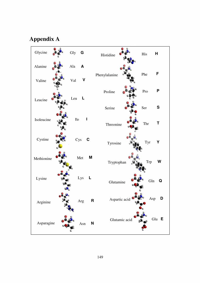
149

Appendix A

Alanine Ala A

Methionine Met M

Glycine Gly G

Valine Val V

Leucine Leu L

Isoleucine Ile I

Cystine Cys C

Lysine Lys L

Arginine Arg R

Asparagine Asn N

Histidine His H

Phenylalanine Phe F

Proline Pro P

Serine Ser S

Threonine Thr T

Tyrosine Tyr Y

Tryptophan Trp W

Glutamine Gln Q

Aspartic acid Asp D

Glutamic acid Glu E

150

Fig. A1. All twenty amino acids with their full name, the structure, followed by three-letter abbreviated name and single letter code. Black dots represent Carbon, red Oxygen, blue Nitrogen, yellow Sulphur and white Hydrogen.

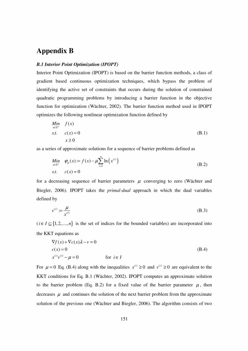
151

Appendix B

B.1 Interior Point Optimization (IPOPT)

Interior Point Optimization (IPOPT) is based on the barrier function methods, a class of

gradient based continuous optimization techniques, which bypass the problem of

identifying the active set of constraints that occurs during the solution of constrained

quadratic programming problems by introducing a barrier function in the objective

function for optimization (Wächter, 2002). The barrier function method used in IPOPT

optimizes the following nonlinear optimization function defined by

( )

. . ( ) 0

0

nx

Min f x

s t c x

x

∈

=

≥

�

(B.1)

as a series of approximate solutions for a sequence of barrier problems defined as

( )( )

1

( ) : ( ) ln

. . ( ) 0

n

ni

xi

Min x f x x

s t c x

µϕ µ∈

=

= −

=

∑� (B.2)

for a decreasing sequence of barrier parameters µ converging to zero (Wächter and

Biegler, 2006). IPOPT takes the primal-dual approach in which the dual variables

defined by

( )( )

:i

iv

x

µ= (B.3)

( { }1,2,....,i I n∈ ⊆ is the set of indices for the bounded variables) are incorporated into

the KKT equations as

( ) ( )

( ) ( ) 0

( ) 0

0 for i i

f x c x v

c x

x v i I

λ

µ

∇ + ∇ − =

=

− = ∈

(B.4)

For 0µ = Eq. (B.4) along with the inequalities ( ) 0ix ≥ and ( ) 0iv ≥ are equivalent to the

KKT conditions for Eq. B.1 (Wächter, 2002). IPOPT computes an approximate solution

to the barrier problem (Eq. B.2) for a fixed value of the barrier parameter µ , then

decreases µ and continues the solution of the next barrier problem from the approximate

solution of the previous one (Wächter and Biegler, 2006). The algorithm consists of two

152

loops, an “outer loop” in which the approximate solution of the barrier problem (Eq. B.2)

satisfies a given tolerance, and an “inner loop” in which Eq. B.4 is solved. IPOPT

converges superlinearly under standard second order sufficiency conditions for the

problem defined in Eq. B.1. For more details on the algorithm and the package, the reader

is requested to consult the IPOPT homepage (www.coin-or.org/Ipopt/) and the following

references (Wächter, 2002, Wächter and Biegler, 2006).

B.2 SCWRL

SCWRL is a side-chain prediction program based on a graph theoretic algorithm. The

graph-theory algorithm is based on representing side chains as vertices in an undirected

graph. Residues having non-zero rotamer interactions energies are considered to have an

edge between the vertices in the graph. Thus, the protein with its rotamers having

interactions with one another can be considered as a big undirected graph. SCWRL uses a

backbone-dependant rotamer library (Dunbrack and Karplus, 1994, Dunbrack and Cohen,

1997, Dunbrack, 2002), an energy function based on the log probabilities of the rotamers

in the library and a repulsive steric energy term. The newer versions of SCWRL (versions

3.0 and above) uses a biconnected graph partitioning algorithm which breaks the large

graph representing the protein into smaller components and then using DEE to solve

(Goldstein, 1994) the best rotamer conformations for each of the smaller components.

The interested reader is requested to refer to the details of the algorithm in the paper by

Dunbrack’s group (Canutescu et al., 2008).

B.3 Nonlinear conjugate gradient method

The conjugate gradient method was first proposed by Hestenes and Stiefel (Hestenes and

Stiefel, 1952) for solving a system of linear equations. Later Fletcher and Reeves

(Fletcher and Reeves, 1964) extended the conjugate gradient method for optimizing

general nonlinear functions. Conjugate gradient methods have low memory requirements

compared to other unconstrained convex optimization solvers like the quasi-Newton

methods (Bazara et al., 1993), and takes at most n iterations to solve an unconstrained

convex problem of n variables.

Let ( )f x be the function to be optimized. We used the nonlinear conjugate

gradient algorithm from the freely available text by Jonathan Richard Shewchuk

153

(www.cs.cmu.edu/~quake-papers/painless-conjugate-gradient.pdf) with minor

modifications, for example, using the Polak-Rebierre formula for β calculation. The

algorithm is presented below.

( ) ( )

( ) ( )

{ }

0;

, _ ;

_ ;

;

( & & & & )

{

, _ ;

;

;

( 0; ; )

{

( 0)

new

old old

new

old

new new old

old old

old

old

iter

f f evalE dEdx x

f Big number

r f

While iter Maxiter r f f

f f evalE dEdx x

d f

r d

for i i N i

if iter

else

δ ε

σ δ

=

∇ =

=

= −∇

< < − <

∇ =

= −∇

=

= < + +

== =

{ }

( ) ( )

_ ( , );

;

, _ ;

;

;

;

;

;

}

1;

}

new new

new new

new old

new

old old

new

old new

line search x d

x x d

f f evalE dEdx x

r f

r r r

r r

r r

d r d

r r

iter iter

σ α

α

α

β

β

=

=

= +

∇ =

= −∇

∆ = −

∆=

= +

=

= +

i

i

In the above algorithm, evalE_dEdx is the function that takes in the vector X (which we

denote by x for simplicity) and returns the function value f and the gradient f∇ evaluated

at X , and N is the size of X . The line_search function calculates α using the following

formula,

154

( )( ) ( )

f x d

f x d d f x dα σ

σ

∇= −

∇ + − ∇

i

i i (B.5)

The parameters , and Maxiter δ ε have values 8 6 31.0 10 , 1.0 10 and 1.0 10− −× × ×

respectively.

B.4 Online Secondary Structure prediction servers

A comprehensive list of online secondary structure prediction servers is given at

http://www.expasy.ch/tools/#secondary. From this website we selected two online

secondary structure prediction servers, namely, the GOR4 secondary structure prediction

server (http://npsa-pbil.ibcp.fr/cgi-bin /npsa_automat.pl?page=npsa_gor4.html, Garnier et

al., 1996), and the HNN server (Guermeur, http://npsa-pbil.ibcp.fr/cgi-bin/

npsa_automat.pl?page=npsa_nn.html) for predicting secondary structures from

sequences.

The GOR method uses the information function defined by,

( | )

( ; ) log( )

P S RI S R

P S

=

(B.6)

where, S is one of the three conformations, i.e. alpha helix (H), beta strand (E) or coil (C),

and R is one of the 20 amino acids. Thus, ( | )P S R is the conditional probability for

observing a conformation S when a residue R is present given by

( | ) ( , ) / ( )P S R P S R P R= , and ( )P S is the probability of observing S. For a large

database with known sequences and secondary structures the above probabilities can be

calculated as ,( , ) /S RP S R f N= , ( ) /RP R f N= , and ( ) /SP R f N= , where N is the total

number of amino acids in the database, ,S Rf is the frequency of residues R observed in

the conformation S in the same database, Rf is the total number of residues R, and

Sf the

total number of residues observed in the conformation S in the same database. Thus,

( )( )

, /( ; ) log

/S R R

S

f fI S R

f N

=

(B.7)

The actual program incorporates corrections for levels of data. For details of the program,

the interested reader is requested to refer to the paper by Robson and co-workers Garnier

et al., 1996).

155

The HNN method (Guermeur, PhD thesis) is based on an ensemble method based on a

multivariate linear regression algorithm which finds estimates of the class posterior

probabilities using optimization and generalized Vapnik-Chernonekis dimensions.

156

Appendix C

Simulation results for the GPU (left) and CPU (right) based tertiary structure prediction

codes. The time is measured in seconds. The function value and the norm are printed

after every 219 (the number of variables in the chosen optimization problem) steps in

optimization (indicate by “iter”) using the nonlinear conjugate optimization program.

This also corresponds to one complete iteration of the linear conjugate gradient part in the

nonlinear conjugate optimization program (see Appendix B3).

157

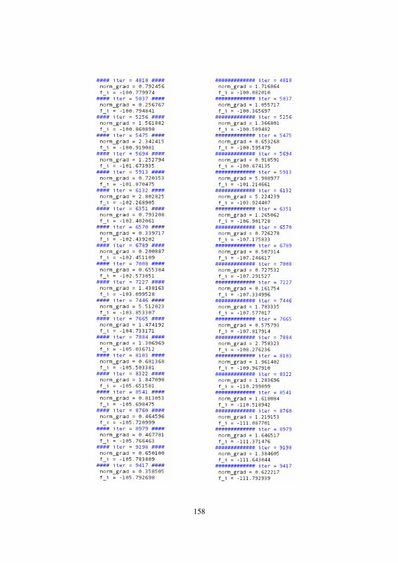
158

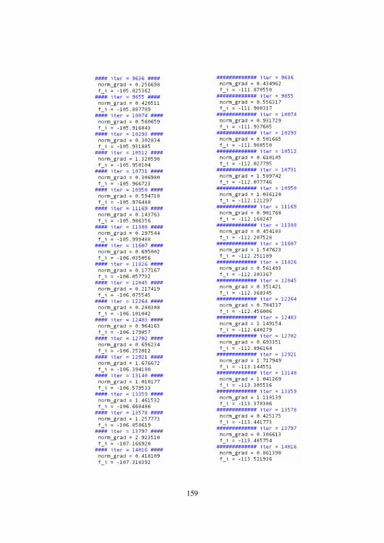
159

160

161

162

163

References

1. Abe, H., and Gō, N., Noninteracting local-structure model of folding and

unfolding transition in globular proteins. II. Application to two-dimensional

lattice proteins, Biopolym., 1981, vol. 20, p.p. 1013-1031.

2. Abkevich, V. I., Gutin, A. M., and Shakhnovich, E. I., Improved design of stable

and fast-folding model proteins. Fold. Desg., 1996, vol. 1, p.p. 221-230.

3. Alvizo, O., and Mayo, S. L., Evaluating and optimizing computational protein

design force fields using fixed composition-based negative design. PNAS, 2008,

vol. 105(34), p.p. 12242-12247.

4. Ananthasuresh, G. K., Protein sequence design on the basis of topology

optimization techniques. IUTAM symposium on topology design optimization of

structures, machines and materials, Ed. Bendsøe, Olhoff N. and Sigmund O.,

Springer, 2006, p.p. 237-248.

5. Anfinsen, C. B., et al., The kinetics of formation of native ribonuclease during

oxidation of the reduced polypeptide chain. PNAS, 1961, vol. 47(9), p.p. 1309-

1314.

6. Anfinsen, C. B., Principles that Govern the Folding of Protein Chains. Science,

1973, vol.181 (4096), p.p. 223-230.

7. Ashby, M. F., and Johnson, K., Materials and Design: The Art and Science of

Material Selection in Product Design, 2002, © Butterworth-Heinemann.

8. Arora, N., and Jayaram, B., Strength of hydrogen bonds in alpha helices. J.

Comput. Chem., vol. 18, no. 9, pp. 1245-1252, 1997.

9. Atilgan, A. R., et al., Anisotropy of fluctuation dynamics of proteins with an

elastic network model. Biophy. J., 2001, vol. 80, p.p. 505-515.

10. Aydin, Z., Altunbasak, Y., and Erdogan, H., Bayesian models and algorithms for

protein beta-sheet prediction. IEEE Trans. Comput. Biol. Bioinfo., 2011, vol. 8,

p.p. 395-409.

11. Ball, K. D., et al., The elastic net algorithm and protein structure prediction. J.

Comput. Chem., 2001, vol. 23, p.p. 77-83.

164

12. Bahar, I., Atilgan, A. R., and Erman, B., Direct Evaluation of thermal fluctuations

in proteins using a single-parameter harmonic potential. Fold. Des., 1997, vol. 2,

p.p. 173-181.

13. Bahar, I., and Jernigan, R. L., Vibrational dynamics of transfer RNAs:

Comparison of the free and synthetase-bound forms. JMB, 1998, vol. 281, p.p.

871-884.

14. Bahar, I., and Rader, A. J., Coarse-grained normal mode analysis in structural

biology. Curr. Op. Struct. Biol., 2005, vol. 15, p.p. 586-592.

15. Baker, D., An exciting but challenging road ahead for computational enzyme

design. Prot. Sci., 2010, vol. 19, p.p. 1817-1819.

16. Bazara, M. S., Sherali, H. D., and Shetty, C. M., Nonlinear Programming Theory

and Algorithms, 2nd Ed., © John Wiley & Sons, Inc.

17. Bernstein, F. C., Koetzle, T.F., Williams, G. J. B., Meyer, Jr. E. F., Brice, M. D.,

Rodgers, J. R., Kennard, O., Shimanouchi, T., and Tasumi, M., The protein data

bank: a computer based archival file for macromolecular structures. JMB, 1977,

vol. 112, p.p. 535-542.

18. Bolon, D. N., and Mayo, S. L., Enzyme-like proteins by computational design.

PNAS, 2001, vol. 98, p.p. 14274-14279.

19. Bowie, J. U., Lüthy, R., and Eisenberg, D., A method to identify protein

sequences that fold into known three-dimensional structure. Science, 1991, vol.

253, p.p. 164-170.

20. Bradley, P. et al, TRILOGS: discovery of sequence-structure patterns across

diverse proteins. PNAS, 2002, vol. 99, p.p. 8500-8505.

21. Brooks, B., and Karplus, M., Harmonic dynamics of proteins: Normal modes and

fluctuations in bovine pancreatic trypsin inhibitor. PNAS, 1983, vol. 80, p.p.

6571-6575.

22. Brown, S., Fawzi, N. J., and Head-Gordon, T., Coarse-grained sequences for

protein folding and design. PNAS, 2003, vol. 100(19), p.p. 10712-17.

23. Bryngelson, J. D., et al., Funnels, pathways, and the energy landscape of protein

folding: a synthesis. Proteins, 1995, vol. 21, p.p. 167-195.

165

24. Bryson, J. W. et al, From Coiled Coils to Small Globular Proteins: Design of a

Native-Like Three-Helix Bundle. Prot. Sci., 1998, vol. 7, p.p. 1404-1414.

25. Butterfoss, G. L., and Kuhlman, B., Computer-based design of novel protein

structures. Ann. Rev. Bioph. Biomol. Strs., 2006, vol. 35, p.p. 49-65.

26. Cannata, N., et al., Simplifying amino acid alphabets by means of a branch and

bound algorithm and substitution matrices. Bioinformatics, 2002, vol. 18, p.p.

1102-1108.

27. Canutescu, A. A., Shelenkov, A. A., and Dunbrack Jr., R. L., A graph-theory

algorithm for rapid protein side-chain prediction. Prot. Sci., 2003, vol. 12, p.p.

2001-2014.

28. Case, D. A., et al., The Amber biomolecular simulation programs. J. Comput.

Chem., 2005, vol. 26, p.p. 1668-1688.

29. Chan, H. S., Folding alphabets. Nature Struct. Biol., 1999, vol. 6 (11), p.p. 994-

996.

30. Chen, J., et al., Increase in the thermostability of the staphylococcal nuclease:

implications for the origin of protein thermostability. JMB, 2000, vol. 303, p.p.

125-130.

31. Chin, T. M., Berndt, K. M., and Yang, N. C., Self-Assembling Hexameric Helical

Bundle Forming peptides. JACS, vol. 114, p.p. 2279-2280.

32. Chiu, T-L., and Goldstein, R. A., Optimizing potentials for inverse protein folding

problem. Prot. Engg., 1998, vol. 11(9), p.p. 749-752.

33. Chotia, C., Principles that Determine the Structure of Proteins. Ann. Rev.

Biochem., 1984, vol53, p.p. 537-572.

34. Cieplak, M., et al, Amino acid classes and protein folding problem. J. Chem.

Phys., 2001, vol. 114, p.p. 1420-1423.

35. Cohen, V. and Parry, D., Alpha-Helical Coiled Coils and Bundles: How to Design

Alpha-Helical protein. Proteins, 1990, vol. 7, p.p. 1-15.

36. Cook, R. D., Malakus, D. S., Plesha, M. E., and Witt, R. J., Concepts and

applications of finite element analysis; Wiley, 2002 edition.

166

37. Cornell, W. D., et al., A second generation force field for the simulation of

proteins, nucleic acids, and organic molecules. J. Am. Chem. Soc., 1995, vol. 117,

p.p. 5179-5197.

38. Cornette, J. L., et al., Hydrophobicity scales and computational techniques for

detecting amphipatic structures in proteins. J. Mol. Biol., 1987, vol. 195, p.p. 659-

685.

39. Dahiyat, B. I., and Mayo, S. L., Protein design automation. Prot. Sci., 1996, vol.

5, p.p. 895-903.

40. Dahiyat, B. I., and Mayo, S. L., De novo protein design: fully automated sequence

selection. Science, 1997a, vol. 278, p.p. 82-87.

41. Dahiyat, B. I., and Mayo, S. L., Probing the role of packing specificity in protein

design. PNAS, 1997b, vol. 94, p.p. 10172-10177.

42. Dahiyat, B. I., Sarisky, C. A., and Mayo, S. L., De novo protein design: towards

fully automated sequence selection. JMB, 1997, vol. 273, p.p. 789-796.

43. Dantas, G., et al., A large scale test of computational protein design: Folding and

stability of nine completely redesigned globular proteins. JMB, 2003, vol. 332,

p.p. 449-460.

44. Das, R., and Baker, D., Macromolecular modeling with Rosetta. Ann. Rev.

Biochem., 2008, vol. 77, pp. 363-382.

45. David, S. R., et al, Functional Rapidly Folding Proteins from Simplified Amino

Acid Sequences. Nat. Struct. Biol., 1997, vol. 4(10), p.p. 805-809.

46. Dayhoff, M. O., Eck, R. V., Park, C. M., A model of evolutionary change in

proteins. Atlas of protein sequence and structure (Ed. M. O. Dayhoff , Maryland:

National Biomedical Research Foundation), 1972, p.p. 89-100.

47. DeGrado, Design of peptides and proteins. Adv. Prot. Chem., 1988, vol. 39, p.p.

51-124.

48. De Grado, W. F., and Lear, J. D., Conformationally constrained alpha-helical

peptide models for protein ion channels, Biopoly., 1990, vol. 29, p.p. 205-213.

49. DeGrado, W. F., Raleigh, D. P., and Handel, T., De novo protein design: what are

we learning ?. Curr. Op. Struct. Biol., 1991, vol. 1, p.p. 984-993.

167

50. DeGrado, W. F., Summa, C. F., Pavone, V., Nastri, F., and Lombardi, A., De

Novo design and Structural Characterization of Proteins and Metalloproteins.

Ann. Rev. Biochem., 1999, vol. 68, p.p. 779-819.

51. Deisenhofer, J., Crystallographic refinement and atomic models of a human FC

fragment and its complex with fragment B of protein A from staphylococcus

areus at 2.9 and 2.8 angstroms resolution. Biochem., 1981, vol. 20, p.p. 2361-

2370.

52. Delarue, M., and Sanejouand, Y.-H., Simplified normal mode analysis of

conformational transitions in DNA-dependant polymerases: the elastic network

model. JMB, 2002, vol. 320, p.p. 1011-1024.

53. Delarue, M., and Dumas, P., On the use of low-frequency normal modes to

enforce collective movements in refining macromolecular structural models.

PNAS, 2004, vol. 101, p.p. 6957-6962.

54. DeMaeyer, M., et al., All in one: a highly detailed rotamer library improves both

accuracy and speed in the modeling of side chains by dead-end elimination. Fold.

Des., 1997, vol. 2, p.p. 53-66.

55. Derrida, B., Random energy model: limit of a family of disordered models. PRL,

1980, vol. 45(2), p.p. 79-82.

56. Desjarlais, J. R., and Handel, T. M., De novo design of the hydrophobic cores of

proteins. Prot. Sci., 1995, vol 4, p.p. 5803-5807.

57. Desjarlais, J. R., and Handel, T. M., Side-chain and backbone flexibility in protein

core design. JMB, 1999, vol. 289, p.p. 305-318.

58. Desjarlais, J. R., and Clarke, N. D., Computer Search Algorithms in Protein

Modofication and Design. Curr. Op. Struct. Biol., 1998, vol. 8, p.p. 471-475.

59. Desmet, J., De Maeyer, M., Hazes, B. and Lasters, I., The dead-end elimination

theorem and its use in protein side-chain positioning. Nature, 1992, vol. 356, p.p.

539-542.

60. Deutsch, J. M., and Kurosky, T., New algorithm for protein design. PRL, 1996,

vol. 76 (2), p.p. 323-326.

61. Dill, K. A., Theory for the folding and stability of globular proteins, . Biochem.,

1985, vol. 24, p.p. 1501-1509.

168

62. Dill, K. A., Dominant Forces in protein Folding. Biochem., 1990, vol. 29 (31),

p.p. 7133-7155.

63. Dill, K. A., and Chan, H. S., From Levinthal to pathways to funnels. Nat. Struct.

Biol., 1997, vol. 4 (1), p.p. 10-19.

64. Dokholyan, N. V., What is protein design alphabet ?. Prot. Struct. Fun. Bioinfo.,

2004, vol. 54, p.p. 622-628.

65. Doruker, P., Jernigan, R. L., and Bahar, I., Dynamics of large proteins through

hierarchical levels of coarse-grained structures. J. Comput. Chem., 2002, vol. 23,

p.p. 119-127.

66. Drexler, K. E., Molecular engineering: An approach to the development of

general capabilities for molecular manipulation. PNAS, 1981, vol. 78(9), p.p.

5275-5278.

67. Dunbrack Jr., R. L., and Karplus, M., Conformational analysis of the backbone-

dependant rotamer preferences of protein sidechains. Nat. Struct. Biol., 1994, vol.

1, p.p. 334-340.

68. Dunbrack Jr., R. L., and Cohen, F. E., Bayesian statistical analysis of protein side-

chain rotamer preferences. Prot. Sci., 1997, vol. 6, p.p. 1661-1681.

69. Dunbrack Jr., R. L., Rotamer libraries in 21st century. Curr. Op. Struct. Biol.,

2002, vol. 12, p.p. 431-440.

70. Dwyer, M. A., Looger, L. L., and Hellinga, H. W., Computational Design of a

Biologically Active Enzyme. Science, 2004, vol. 304, p.p. 1967-1971.

71. Eichinger, B. E., Elasticity theory I. Distribution function for perfect phantom

networks. Macromol., 1972, vol. 5, p.p. 496-505.

72. Erman, B. , Bahar, I., and Jernigan, R. L., Equilibrium states of rigid bodies with

multiple interaction sites: Application to protein helices. J. Chem. Phys., 1997,

vol. 107, no. 6, pp. 2046-2058.

73. Erman, B., and Dill, K., Gaussian model of protein folding. J. Chem. Phys., 2000,

vol. 112(2), p.p. 1050-1056.

74. Farinas, E., and Regan, L., The de novo design of a rubredoxin-like Fe site. Prot.

Sci., 1998, vol. 7, p.p. 1939-1946.

169

75. Fletcher, R., and Reeves, C., Function minimization by conjugate gradients,

Computer J., 1964, vol. 7, p.p. 149-154.

76. Flory, P. J., Statistical thermodynamics of random networks. Proc. Roy. Soc. A.,

1976, vol. 351, p.p. 351-380.

77. Floudas, C. A., Fung, H. K., McAllister, H. R., Mönnigmann, M., and Rajgaria,

R., Advances in protein structure prediction and de novo protein design: a review.

Chem. Engg. Sci., 2006, vol. 61, p.p. 966-988.

78. Fraternali, F., and van Gunsteren, W. F., An efficient mean solvation force model

for use in molecular dynamics simulations of proteins in aqueous solution. JMB,

1996, vol. 256, p.p. 939-948.

79. Fung, H. K., Welsh, W. J., and Floudas, C. A., Computational de novo peptide

and protein design: Rigid templates versus flexible templates. Ind. Eng. Chem.

Res., 2008, vol. 47, p.p. 993-1001.

80. Garnier, J., et al., GOR secondary structure prediction method version IV.

Methods in Enzymology, 1996, Ed. Doolittle, R. F., vol. 266, p.p. 540-553.

81. Ghadiri, M. R., et al., Self-assembling organic nanotubes based on a cyclic

peptide architecture. Nature, 1993, vol., 366, p.p. 324-327.

82. Gillespie, B., et al., NMR and temperature junp measurements of de novo

designed proteins demonstrate rapid folding in the absence of expilict selection

for kinetics. JMB, 2003, vol. 330, p.p. 813-819.

83. Gibney, B. R. et al, Synthesis of novel proteins. Curr. Op. Chem. Biol., 1997, vol.

1, p.p. 537-542.

84. Gō, N., Noguti, T., and Nishikawa, T., Dynamics of small globular proteins in

terms of low-frequency vibrational modes. PNAS, 1983, vol. 80, p.p. 3690-3700.

85. Goffe, W. L., Ferrier, G. D., and Rogers, J., Global optimization of statistical

functions with simulated annealing. J. Econometrics, 1994, vol. 6, p.p. 65-99.

86. Goldstein, R. F., Efficient rotamer elimination applied to protein side chains and

related spin glasses. Biophys. J., 1994, vol. 66, p.p. 1335-1340.

87. Gordon, D. B., and Mayo, S. L., Radical performance enhancements for

combinatorial optimization algorithms based on the dead-end elimination

theorem. J. Comput. Chem., 1998, vol. 19(13), p.p. 1505-1514.

170

88. Gordon, D. B., Marshall, S. A., and Mayo, S. L., Energy functions for protein

design. Curr. Op. Struct. Biol., 1999, vol. 9, p.p. 509-513.

89. Gordon, D. B., and Mayo, S. L., Branch-and-Terminate: a combinatorial

optimization algorithm for protein design. Structure, 1999, vol. 7, p.p. 1089-1098.

90. Grove, A., et al., A molecular blueprint for the pore-forming structure of voltage-

gated ion channels, PNAS, 1991, vol. 88, p.p. 6418-6422.

91. Guermeur, Y., Combinaison de classifieurs statistiques, Application a la

prediction de structure secondaire des proteins. PhD Thesis. (http://npsa-

pbil.ibcp.fr/NPSA/npsa_references.html#hnn)

92. Güner, U., Arkun, Y., and Erman, B., Optimum folding pathways of proteins:

their determination and properties. J. Chem. Phys., 2006, vol. 124, 139411(1-12).

93. Gutte, B., et al.,

94. Halilgolu, T., Bahar, I., and Erman, B., Gaussian dynamics of folded proteins.

PRL, 1997, vol. 79(16), p.p. 3090-3093.

95. Halilgolu, T., et al., How similar are protein folding and protein binding nuclei?

Examination of vibrational motions of energy hot spots and conserved residues.

Biophys. J., 2005, vol. 88, p.p. 1552-1559.

96. Hao, M-H, and Scheraga, H. A., Designing potential energy functions for protein

folding. Curr. Op. Struct. Biol., 1999, vol. 9, p.p. 184-188.

97. Harbury, P. B., et al, High-Resolution Protein Design with Backbone Freedom.

Science, 1998, vol. 282, p.p. 1462-1467.

98. He, J., et al., Efficiently explore the energy landscape of proteins in molecular

dynamics simulations by amplifying collective motions. Biophys. J., 2003, vol.

119, p.p. 4005-4017.

99. Hecht, M. H., et al, De Novo Design, Expression, and Characterization of Felix:

A Four-Helix Bundle Protein of Native-Like Sequence. Science, 1990, vol. 249,

p.p. 884-891.

100. Hecht, M. H., De novo design of beta-sheet proteins. PNAS, 1994, vol. 91, p.p.

8729-8730.

101. Hecht, M. H., Strategies for the Design of Novel Proteins. Protein Engineering

and Design, 1996, Academic Press Inc., Ed. Carey, P. R., p.p. 1-46.

171

102. Hedstrom, L., Converting trypsin to chymotrypsin: the role of surface loops,

Science, 1992, vol. 255, p.p. 1249-1253.

103. Heinkoff, S., and Heinkoff, J. G., Amino acid substitution matrices from protein

blocks. PNAS, 1992, vol. 89, p.p. 10915-10919.

104. Hellinga, H. W., et al., Construction of ligand binding sites in proteins of known

structure. II: Grafting of a buried transition metal binding site into E.Coli

thioredoxin. JMB, 1991, vol. 222, p.p. 787-803.

105. Hellinga, H. W., and Richards, F. M., Optimal sequence selection in proteins of

known structure by simulated evolution. PNAS, 1994, vol. 91, p.p. 5803-5807.

106. Hellinga, H. W., Rational protein design: Combining theory and experiment.

PNAS, 1997, vol. 94, p.p. 10015-10017.

107. Hess, B., et al, GROMACS 4: Algorithms for Highly Efficient, Load-Balanced,

and Scalable Molecular Simulation. J. Chem. Theory & Comput., 2008, vol.

4(2), pp. 435-447.

108. Hestenes, M. R., and Stiefel, E., Methods of conjugate gradients for solving

linear systems, J. Res. National Bereau of Standards, 1952, vol. 49, p.p. 409-

436.

109. Higgins, D. G., and Sharp, P. M., CLUSTAL: a package for performing multiple

sequence alignment on a microcomputer. Gene, 1988, vol. 73, p.p. 237-244.

110. Hill, T. L., An Introduction to Statistical Thermodynamics, © Dover, 1986.

111. Ho, S. P. , and DeGrado, W. F., Design of a 4-Helix Bundle Protein: Synthesis

of Peptides which Self-Associate into a Helical Protein. JACS, 1987, vol. 109,

p.p. 6751-6758.

112. Hodges, R. S. et al, Synthetic Model Proteins: Contribution of Hydrophobic

Residues and Disulphide Bonds to Protein Stability. Pep. Res., 1990, vol. 3, p.p.

123-137.

113. Holland, J. H., Adaptation in natural and artificial systems. 1992, © MIT press.

114. Horton et al, Principles of Biochemistry, 4th Ed. © Pearson Education Inc.

115. Irbäck, A., Peterson, C., Potthast, F., and Sandelin, E., Monte Carlo procedure

for protein design. PRL E, 1998, vol. 58 (5), p.p. 5249-52.

172

116. Inaka, K., et al., Crystal structures of the apo- and holomutant human lysozymes

with an introduced Ca2+ binding site. J. Biol. Chem., 1991, vol. 266, p.p.

20666-20671.

117. Jaenicke, R., et al., Conformation of a synthetic 34-residue polypeptide that

interacts with nucleic acids. FEBS Lett., 1980, vol. 114, p.p. 161-164.

118. Jernigan, R. L., and Bahar, I, Structure-derived potentials and protein

simulations. Curr. Op. Struct. Biol., 1996, vol. 6, p.p. 195-209.

119. Jha, A. N., Ananthasuresh, G. K., and Vishveshwara, S., Protein sequence

design based on the topology of the native state structure. J. Theo. Biol., 2006,

vol. 248, p.p. 81-90.

120. Jha, A. N., Ananthasuresh, G. K., and Vishveshwara, S., A search for energy

minimized sequences of proteins. PLOS 1, 2009, vol. 4(8), e6684.

121. Jiang, L., et al, De novo computational design of retro-aldol enzymes. Science,

2008, vol. 319, p.p. 1387-1391.

122. Johnson, R. A., and Wichern, Applied Multivariate Statistical Analysis, 2006, ©

Pearson Education Inc.

123. Keller, D. A., et al., Finding global minimum: a fuzzy end elimination

implementation. Prot. Engg., 1995, vol. 8, p.p. 893-904.

124. Kim., M. K., Chirikjian, G. S., and Jernigan, R. L., Elastic models of

conformational transitions in macromolecules. J. Mol. Graph. Model., 2002, vol.

21, p.p. 151-160.

125. Kim, M. K., Jernigan, R. L., and Chirikjian, G. S., An elastic network model of

HK97 capsid maturation, J. Struct. Biol., 2003, vol. 143, p.p.107-117.

126. Kirk, D. B., and Hwu, W., Programming Massively Parallel Processors A

Hands-on Approach, 2010, © Elsevier Inc.

127. Kissinger, C. R., et al., Crystal structure of an engrailed homeodomain/DNA

complex at 2.8 angstroms resolution: a framework for understanding

homeodomain/DNA interactions. Cell, 1990, vol. 63, p.p. 579-590.

128. Klauser, S., et al., Structure-function studies of designed DDT-binding

polypeptides. Biochem. Biophys. Res. Comm., 1991, vol. 179, p.p. 1212-1219.

173

129. Klepeis, J. L., and Floudas, C. A., ASTRO-FOLD: A combinatorial and global

optimization framework for ab initio prediction of three-dimensional structures

of proteins from amino acid sequences. Biophys. J., 2003, vol. 85, p.p. 2119-

2146.

130. Klepeis, J. L., and Floudas, C. A., Prediction of β -sheet topology and

disulphide bridges in polypeptides. J. Comput. Chem., vol. 24, pp. 191-208,

2003.

131. Koehl, P., and Delarue, M., Application of self-consistent mean-field theory to

predict proteins side-chains conformation and estimate their conformational

entropy. JMB, 1994, vol. 239, p.p. 249-275.

132. Koehl, P., and Levitt, M., De novo protein design. I. In search of stability and

specificity. JMB, 1999a, vol. 293, p.p. 1161-1181.

133. Koehl, P., and Levitt, M., De novo protein design. II. Plasticity in sequence

space. JMB, 1999a, vol. 293, p.p. 1183-1193.

134. Koehl, P., and, Levitt, M., Improved recognition of native-like protein structures

using a family of designed sequences. PNAS, 2002, vol. 99(2), p.p. 691-696.

135. Koh, S. K., Ananthasuresh, G. K. and Vishveshwara S., A deterministic

optimization approach to protein sequence design using continuous models. Int.

J. Rob. Res., 2005, vol. 24, p.p. 109-130.

136. Koh, S. K., Ananthasuresh, G. K., and Croke, C., A quadratic programming

formulation for the design of reduced protein models in continuous sequence

space. J. Mech. Des., 2005, vol. 127, p.p. 728-734.

137. Koh, S. K., Guangjun, L., and Zhu, W-H, A continuous protein design model

using artificial power law in topology optimization. J. Mech. Des., 2009, vol.

131, 041001.

138. Koisol, C., Goldman, N., and Buttimore, H. N., A new criteria and method for

amino acid classification. J. Theo. Biol., 2004, vol. 228, p.p. 97-106.

139. Kono, H., and Doi, J., Energy minimization method using automata network for

sequence and side-chain conformation prediction from given backbone

geometry. Proteins, 1994, vol. 19, p.p. 244-255.

174

140. Kono, H., and Saven, J. G., Statistical theory for protein combinatorial libraries.

Packing interactions, backbone flexibility and sequence variability of a main-

chain structure. JMB, 2001, vol. 306, p.p. 607-628.

141. Kraemer-Pecore C. M., et al, Computational Protein design, Curr. Op. Chem.

Biol., 2001, vol. 5, p.p. 690-695.

142. Krebs et al., Normal mode analysis of macromolecular motions in a database

framework: developing mode concentration as a useful classifying statistic.

Proteins, 2002, vol. 48, p.p. 682-695.

143. Kruskal J. B., and Wish M., Multidimensional Scaling,1978, Sage publications.

144. Kuhlman, B., O’Neill, J. W., Kim, D. E., Zhang, K. Y., and Baker, D., Accurate

computer-based design of new backbone conformation in the second turn of

protein L. JMB, 2002, vol. 315, p.p. 471-477.

145. Kuhlman, B., Dantas, G., Ireton, G. C., Varani, G., Stoddard ,B. L., and Baker,

D., Design of a novel globular protein fold with atomic-level accuracy. Science,

2003, vol. 302, p.p. 1364-1368.

146. Kundu, S., et al., Automatic domain decomposition of proteins by a Gaussian

network model. Proteins, 2004, vol. 57, p.p. 725-733.

147. Kundu, S., and Jernigan, R. L., Molecular mechanism of domain swapping in

proteins: an analysis of slower motions. Biophys. J., 2004, vol. 86, p.p. 3846-

3854.

148. Kurkcuoglu, O., et al., Mixed levels of coarse graining of large proteins using

elastic network model succeeds in extracting the slowest motions. Polym., 2004,

vol. 45, p.p. 649-657.

149. Kuroki, R., et al., Design and creation of a Ca2+ binding site in human

lysozyme to enhance structural stability. PNAS, 1989, vol. 86, p.p. 6903-6907.

150. Larson et al., Thoroughly sampling sequence space: Large-scale protein design

of structural ensembles. Prot. Sci., 2002, vol. 11, p.p. 2804-2813.

151. Lassila, J. K., Conformational diversity and computational enzyme design. Curr.

Op. Chem. Biol., 2010, vol. 14, p.p. 676-682.

175

152. Lasters, I., De Maeyer, M. and Desmet, J., Enhanced dead-end elimination in the

search for global minimum energy conformation of a collection of protein

sidechains. Prot. Engg., 1995, vol. 8, p.p. 815-822.

153. Lazar, et al., De novo design of the hydrophobic core of ubiquitin. Prot. Sci.,

vol. 6, p.p. 1167-1178.

154. Lee, C., and Levitt, M., Accurate prediction of the stability and activity effects

of site-directed mutagenesis on a protein core. Nature, 1991, vol. 352, p.p. 448-

451.

155. Lee C., Predicting protein mutant energetics by self-consistent ensemble

optimization. JMB, 1994, vol. 236, p.p. 918-939.

156. Leo-Macais et al., An analysis of core deformations in protein superfamilies.

Biophys. J., 2005, vol. 88, p.p. 1291-1299.

157. Lerner, R. A., et al., At the crossroads of chemistry and immunology: catalytic

antibodies. Science, 1991, vol. 252, p.p. 659-667.

158. Levitt, M., and Warshel, A., Computer simulation of protein folding. Nature,

1975, vol. 253, p.p. 694-698.

159. Levitt, M., A Simplified Representation of Protein Conformations for rapid

Simulation of Protein Folding. JMB, 1976, vol. 104, p.p. 59-107.

160. Levitt, M., Protein Folding by Restrained Energy Minimization and Molecular

Dynamics. JMB, 1983, vol. 170, p.p. 723-764.

161. Levitt, M., Sander, C., and Stren, P. S., Protein normal mode dynamics: Trypsin

inhibitor, Crambin, Ribonuclease and Lysozyme. JMB, 1885, vol. 181, p.p. 423-

447.

162. Li, H., Tang, C., and Wingreen, N. S., Nature of driving force for protein

folding: A result from analyzing statistical potential. Phy. Rev. Lett., 1997, vol.

79(4), p.p. 765-768.

163. Li, G., and Cui, Q., A coarse-grained normal mode approach for

macromolecules: an efficient implementation and application to Ca2+-ATPase.

Biophys. J., 2002, vol. 83, p.p. 2457-2474.

164. Liang, S., and Grishin, N. V., Effective scoring functions for protein sequence

design. Prot. Struct. Fun. Bioinfo., 2004, vol. 54, p.p. 271-281.

176

165. Liwo, A., et al., A United-Residue Force Field for Off-Lattice Protein-Structure

Simulations. I. Functional forms and parameters of long-range side-chain

interaction potentials from protein crystal data. J. Comput. Chem., 1997a, vol.

18, p.p. 849-873.

166. Liwo, A., et al., A United-Residue Force Field for Off-Lattice Protein-Structure

Simulations. II. Parameterization of short-range interactions and determination

of weights of energy terms by Z-score optimization. J. Comput. Chem., 1997b,

vol. 18, p.p. 874-887.

167. Looger, L. L., and Hellinga, H. W., Generalized dead-end elimination

algorithms make large-scale protein side-chain structure prediction tractable:

implications for protein design and structural genomics. JMB, 2001, vol. 307,

p.p. 429-445.

168. Looger, L. L., Dwyer, M. A., Smith, J. J., and Hellinga, H. W., Computational

design of receptor and sensor proteins with novel functions, Nature, 2003, vol.

423, p.p.185-190.

169. Luan, C. H., et al., Differential scaning calorimetry studies of NaCl effect on the

inverse temperature transition of some elastin-based polytetra-, polypenta-, and

polynanopeptides. Biopoly., 1991, vol. 31, p.p. 465-475.

170. Luenberger, D. G., Linear and non-linear programming; 2nd Ed. © Springer

Verlag.

171. Luthra, A., Jha, A. N., Ananthasuresh, G. K. and Vishveshwara, S., A Method

for Computing the Inter-Residue Interaction Potentials for reduced Amino Acid

Alphabet. J. Biosci., 2007, vol. 32 (5), p.p. 883-889.

172. Malakauskas, S. M., and Mayo, S. L., Design, structure and stability of a

hyperthermophilic protein variant. Nat. Struct. Biol., 1998, vol. 5, p.p. 470-475.

173. Mandell, D. J., and Kortemme, T., Backbone flexibility in computational protein

design. Curr. Op. Biotech., 2009, vol. 20, p.p. 420-428.

174. Mead, A., Review of the development of Multidimensional Scaling methods.

The Statistician, 1992, vol. 41 (1), p.p. 27-39.

175. Mendes, J., Guerois, R., and Serrano, L., Energy estimation in protein design.

Curr. Op. Struct. Biol., 2002, vol. 12, p.p. 441-446.

177

176. Metropolis, N., Rosenbluth, A. W., Rosenbluth, M. N., Teller, A. H., and Teller,

E., Equations of state calculations by fast computing machines. J. Chem. Phys.,

1953, vol. 21, p.p. 1087-1092.

177. Micheletti, C., et al., Elastic properties of proteins: insight on the folding process

and evolutionary selection of native structures. JMB, 2002, vol. 321, p.p. 909-

921.

178. Mirny, L., and Shakhnovich, E., How to derive a protein folding potential: A

new approach to an old problem. JMB, 1996, vol. 264, p.p. 1164-1179.

179. Mirny, L., and Shakhnovich, E., Universally conserved positions in protein

folds: reading evolutionary signals about stability, folding kinetics and function.

J. Mol. Biol, 1999, vol. 291, p.p. 177-196.

180. Mirny, L., and Shakhnovich, E., Evolutionary conservation of the folding

nucleus. J. Mol. Biol, 2001, vol. 308, p.p. 123-129.

181. Mirny, L., and Shakhnovich, E., Protein folding theory: from lattice to all atom

models. Ann. Rev. Biophys. Biomol. Struct., 2001, vol. 30, p.p. 361-396.

182. Miyazawa, S. and Jernigan. R. L., Estimation of effective interresidue contact

energies from protein crystal structures: quasi-chemical approximation.

Macromol., 1985, vol. 18, p.p. 534-552.

183. Miyazawa, S. and Jernigan, R. L., Residue-residue Potentials with a Favorable

Contact Pair term and an Unfavorable High Packing Density Term, for

Simulation and Threading. JMB, 1996, vol. 256, p.p. 623-644.

184. Miyashita, O., Wolynes, P. G., and Onuchic, J. N., Simple energy landscape

model for the kinetics of functional transitions in proteins. J. Phys. Chem. B.,

2005, vol. 109, p.p. 1959-1969.

185. Miyata, T., Miyazawa, S., and Yasunaga, T., Two types of amino acid

substitutions in protein evolution. J. Mol. Evol., 1979, vol. 12, p.p. 219-236.

186. Moffet, D. A., and Hecht, M. H., De novo proteins from combinatorial libraries.

Chem. Rev., 2001, vol. 101, p.p. 3191-3203.

187. Mondragon, A., Wolberger, C., and Harrison, S. C., Structure of phage 434 cro

protein at 2.35 angstroms resolution. JMB, 1989 b, vol. 205, p.p. 179-188.

178

188. Moser, R., et al., An artificial crystalline DDT-binding polypeptide. FEBS Lett.,

1983, vol. 157, p.p. 247-251.

189. Moult, J., Comparison of database potentials and molecular mechanics force

fields. Curr. Op. Struct. Biol., 1997, vol. 7, p.p. 194-199.

190. Morrissey, M. P., and Shakhnovich, E. I., Design of proteins with selected

thermal properties. Fold. Desg., 1996, vol. 1, p.p. 391-405.

191. Murphy, R. L., Wallqvist, A., and Levy, M. R., Simplified amino acid alphabets

for protein fold recognition and implications for folding. Prot. Engg., 2000, vol.

13, p.p. 149-152.

192. Nanias, M. , et al., Packing helices in proteins by global optimization of a

potential energy function. PNAS, 2003, vol. 100, no. 4, pp. 1706-1710.

193. Nelson, D. L., and Cox, M. M., Principles of Biochemistry, 5th Ed. © W. H.

Freeman and Company.

194. Offredi, F., et al., De novo backbone and sequence design of an idealized /α β -

barrel protein: evidence of stable tertiary structure. JMB, 2003, vol. 325, p.p.

163-174.

195. Oiki, S., et al., Bundles of amphiphatic transmembrane alpha-helices as a

structural motif for ion-conducting channel proteins: Studies on sodium

channels and acetylcholine receptors. Proteins, 1990, vol. 8, p.p. 226-236.

196. Onuchic, J. N., Luthey-Schulten, Z., and Wolynes, P. G., Theory of Protein

Folding: The Energy Landscape Perspective. Ann. Rev. Phys. Chem., 1997, vol.

48, p.p. 545-600.

197. Pande, V. S., Grosberg, A. Y., and Tanaka, T., Statistical mechanics of simple

models of protein folding and design. Biophys. J., 1997, vol. 73, p.p. 3192-3210.

198. Papalambros, P. P. and Wilde, D. J., Principles of optimal design – modeling

and computation. Cambridge University Press, 2000.

199. Pedersen, J. T., and Moult, J., Genetic algorithms for protein structure

prediction. Curr. Op. Struct. Biol., 1996, vol. 6, p.p. 227-231.

200. Pettersen et al., UCSF Chimera – a visualization system for exploratory research

analysis. J. Comput. Chem., 2004, vol. 25(13), p.p. 1605-1612.

179

201. Pierce, N. A., et al., Conformational splitting: a more powerful criterion for

dead-end elimination. J. Comput. Chem., 2000, vol. 21, p.p. 999-1009.

202. Plaxco, K. W., et al, Simplified proteins: minimalist solutions to the ‘protein

folding problem’. Curr. Op. Struct. Biol., 1998, vol. 8, p.p. 80-85.

203. Pokala, N., and Handel, T. M., Review: Protein design — Where We Were,

Where We Are, Where We’re Going. J. Struct. Biol., 2001, vol. 139, p.p. 269-

281.

204. Ponder, J. W., and Richards, F. M., Tertiary templates for proteins Use of

Packing criteria in the enumeration of allowed sequences for different structural

classes. JMB, 1987, vol. 193, p.p. 775-791.

205. Ptitsyn, O. B., and Ting, K. L. H., Non-functional conserved residues in globins

and their possible role as a folding nucleus. JMB, 1999, vol. 291, p.p. 671-682.

206. Quinn, T. P. et al, Betadoublet: De novo design, synthesis, and characterization

of a beta-sandwich protein. PNAS, 1994, vol. 91, p.p. 8487-8751.

207. Rader, A. J., and Bahar, I., Folding core predictions from network models of

proteins. Polym., 2004, vol. 45, p.p. 659-668.

208. Rader, A. J., et al., Identification of core amino acids stabilizing rhodopsin.

PNAS, 2004, vol. 101, p.p. 7246-7251.

209. Rader, A. J. et al., Maturation dynamics of HK97 bacteriophage capsid. Struct.,

2005, vol. 13, p.p. 413-421.

210. Raha, K., Wollacott, A. M., Italia, M. J., and Desjarlais, J. R., Prediction of

amino acid sequence from structure. Prot. Sci., 2000, vol. 9, p.p. 1106-1119.

211. Rakshit, S., and Ananthasuresh, G. K., An amino acid map of inter-residue

contact energies using metric multi-dimensional scaling. J. Theo. Biol., 2008,

vol. 250, p.p. 291-297.

212. Rakshit, S., and Ananthasuresh, G. K., A novel approach for large-scale

polypeptide folding based on elastic networks using continuous optimization. J.

Theo. Biol., 2010, vol. 262, p.p. 488-497.

213. Ramachandran, G. N., Ramakrishnan, C., Sasisekharan, V., Stereochemistry of

polypeptide chain configurations. JMB, 1963, vol. 7, p.p. 95-99.

180

214. Regan, L., and DeGrado, W. F., Characterization of Helical protein designed

from First Principles. Science, 1988, vol. 241, p.p. 976-978.

215. Rothlisberger, D., et al, Kemp elimination catalysis by computational enzyme

design. Nature, 2008, vol. 453, p.p. 190-195.

216. Roux, B., and Karplus, M., The normal modes of the Gramacidin-A dimmer

channel. Biophys. J., 1988, vol. 53, p.p. 297-309.

217. Sali, A., and Blundell, T. L., Comparative protein modeling by satisfaction of

spatial restraints. JMB, 1993, vol. 234, pp. 779-815.

218. Sancho, D. D., et al., Evolutionary Method for the Assembly of rigid protein

Elements. J. Comput. Chem., 2004, vol. 26, pp. 131-141.

219. Sander, C., Design of protein structures: helix bundles and beyond. Trends.

Biotech., 1994, vol. 12, p.p. 163-167.

220. Saven, J. G., and Wolynes, P. G., Statistical Mechanics of The Combinatorial

Synthesis and Analysis of Folding Macromolecules. J. Phys. Chem. B, 1997,

vol. 101, p.p. 8375-8389.

221. Saven, J. G., Combinatorial protein design. Curr. Op. Struct. Biol., 2002, vol.

12, p.p. 453-458.

222. Schueler-Furman, O., et al, Progress in Modeling of Protein Structures and

Interactions. Science, 2005, vol. 310, p.p. 638-642.

223. Schulz, G. E., and Schirmer, R. H., Principles of Protein Structure., Ed. Charles

R Cantor, (Springer advanced texts in chemistry) © Springer Verlag , 1979, pp.

10-16.

224. Schuyler, A. D., and Chirikjian, G. S., Normal mode analysis of proteins: a

comparison of rigid cluster modes with C-alpha coarse graining. J. Mol. Graph.

Model., 2004, vol. 22, p.p. 183-193.

225. Scrutton, N. S., et al., Redesign of the coenzyme specificity of a dehydrogenase

by protein engineering. Nature, vol. 343, p.p. 38-43.

226. Schwartz, R. M. and Dayhoff, M. O., Matrices for detecting distant

relationships. Atlas of Prot. Struct., 1978, vol. 5, p.p. 353-358.

227. Shakhnovich, E. I., and Gutin, A. M., Engineering of stable and fast-folding

sequences of model proteins. PNAS, 1993, vol. 90, p.p. 7195-7199.

181

228. Seno, F., et al., Optimal protein design procedure. PRL, 1996, vol. 77 (9), p.p.

1901-1904.

229. Shen, Y., et al., Intrinsic flexibility and gating mechanism of the potassium

channel KcsA. PNAS, 2002, vol. 99(4), p.p. 1949-1953.

230. Shewchuk, J. R., 1994, www.cs.cmu.edu/~quake-papers/painless-conjugate-

gradient.pdf (as on 28th December, 2009).

231. Shafmeister, C. E., et al, A designed four helix bundle protein with native-like

structure. Nat. Struct. Biol., 1997, vol. 4(12), p.p. 1039-1046.

232. Shafmeister, C. E., and Stroud, R. M., Helical protein design. Curr. Op.

Biotech., 1998, vol. 9, p.p. 350-353.

233. Shakhnovich, E. I., and Gutin, A. M., Engineering of stable and fast-folding

sequences of model proteins. PNAS, 1993, vol. 90, p.p. 7195-7199.

234. Siegel et al, Computational design of an enzyme catalyst for a stereoselective

biomolecular Diels-Alder reaction. Science, 2010, vol. 329, p.p. 309-314.

235. Simons, K. T., Kooperberg, C., Huang, E., and Baker, D., Assembly of protein

tertiary structures from fragments with similar local sequences using simulated

annealing and Bayesian scoring functions. JMB, 1997, vol. 268, p.p. 209-225.

236. Sinha, K. K. and Udgaonkar, J. B. Early events in protein folding. Curr. Sc.,

2009, vol. 96 (8), pp. 1053-1070.

237. Sippl, M. J., Calculation of conformational ensembles from potentials of mean

force. An approach to the knowledge-based prediction of local structures in

globular proteins. JMB, 1990, vol. 213, p.p. 859-883.

238. Sluka, J. P. et al., Synthesis of a sequence-specific DNA-cleaving peptide.

Science, 1987, vol. 238, p.p. 1129-1132.

239. Srivastava, I., and Bahar, I., Common mechanism of pore opening shared by

five different potassium channels. Biophys. J., 2006, vol. 90, p.p. 3929-3940.

240. Street, A. G., and Mayo, S. L., Computational protein design. Structure, 1999,

vol. 7(5), p.p. 105-109.

241. Su, A., and Mayo, S. L., Coupling backbone flexibility and amino acid sequence

selection in protein design. Prot. Sci., 1997, vol. 6, p.p. 1701-1707.

182

242. Svensson, L. A., Thulin, E., and Forsen, S., Proline cis-trans isomers in

calbindin D9K observed by X-ray crystallography. JMB, 1992, vol. 223, p.p.

601-606.

243. Sym, L., Taneja, A. K., and Hodges, R. S., Synthesis of a model protein of

defined secondary and quaternary structure. J. Bio. Chem., 1984, vol. 259, p.p.

13253-13261.

244. Szarecka, A., Xu, Y, and Tang, P., Dynamics of heteropentameric nicotinic

acetylcholine receptor: Implications of the gating mechanism. Proteins, 2007,

vol. 68, p.p. 948-960.

245. Taly, A., et al., Normal mode analysis suggests a quaternary twist model for the

nicotinic receptor gating mechanism, Biophys. J., 2005, vol. 88, p.p. 3954-3965.

246. Tama, F., et al., Building-block approach for determining low-frequency normal

modes of macromolecules. Proteins, 2000, vol. 41, p.p. 1-7.

247. Tama, F., et al., Exploring global distortions of biological macromolecules and

assemblies from low-resolution structural information and elastic network

theory. JMB, 2002, vol. 321, p.p. 297-305.

248. Tama, F., and Brooks III, C. L., Diversity and identity of mechanical properties

of icosahedral viral capsids studied with elastic network normal mode analysis.

JMB, 2005, vol. 345, p.p. 299-314.

249. Tanaka, S., and Scheraga, H. A., Medium- and long-range interaction

parameters between amino acids for predicting three-dimensional structures for

proteins. Macromol., 1976, vol. 9, p.p. 945-950.

250. Tatsumi, R., et al., A hybrid method of molecular dynamics and harmonic

dynamics for docking of flexible ligand to flexible receptor. J. Comput. Chem.,

2004, vol. 25, p.p. 1995-2005.

251. Tirion, M. M., Large amplitude elastic motions in proteins from a single-

parameter, atomic analysis. PRL, 1996, vol. 27(9), p.p. 1905-1908.

252. Thomas, P. D., and Dill, K. A., Statistical Potentials Extracted from Protein

Structures: How accurate are they ?. JMB, 1996, vol. 257, p.p. 457-469.

253. Torgerson, W. S., Multidimensional Scaling: I. Theory and Method.

Psychometrica, 1952, vol. 17 (4), p.p. 401-419.

183

254. Tozzini, V., Coarse-grained models for proteins. Curr. Op. Struct. Biol., 2005,

vol. 15, p.p. 144-150.

255. Tozzini, V., and Rocchia, W., Mapping All-Atom Models onto One-Bead

Coarse-Grained Models: General Properties and Applications to a Minimal

Polypeptide Model. J. Chem. Theory Comput., vol. 2, pp. 667-673, 2006.

256. Tozzini, V., Multiscale modeling of proteins. Acc. Chem. Res., 2010, vol. 43(2),

p.p. 220-230.

257. Tozzini, V., Minimalist models for proteins: a comparative analysis. Quat. Rev.

Biophy., 2010, vol. 43(3), p.p. 333-371.

258. Trylska, J., et al., Exploring global motions and correlations in the ribosome.

Biophys. J., 2005, vol. 89, p.p. 1455-1463.

259. Tuffery, P., et al, A new approach to the rapid determination of protein side

chain conformations. J. Biomol. Struct. Dyn, 1991, vol. 8, p.p. 1267-1269.

260. Valadie et al., Dynamical Properties of the MscL of Escherichia coli: A normal

mode analysis. JMB, 2003, vol. 332, p.p. 657-674.

261. Venkatarajan, M. S., and Braun, W., New quantitative descriptors of amino-

acids based on multidimensional scaling of a large number of physical-chemical

properties. J. Mol. Model, 2001, vol. 7, p.p. 445-453.

262. Ueda, Y., Taketomi, H., and Gō, N., Studies on protein folding, unfolding, and

fluctuations by computer simulation. II. A three-dimensional lattice model of

Lysozyme. Macromol., 1978, vol. 17, p.p. 1531-1548.

263. Urry, D. W., Protein Folding: Deciphering the Second Half of the Genetic Code.

American Assoc. for the Advancement of Science (Eds. L. Gierasch and J. King),

1990, p.p. 63-67.

264. Voigt, C. A., Gordon, D. B., and Mayo, S. L., Trading accuracy for speed: A

Quantitative Comparison of Search algorithms in Protein Sequence Design.

JMB, 2000, vol 299, p.p. 789-803.

265. Wächter, A., An Interior Point Algorithm for Large-Scale Nonlinear

Optimization with Applications in Process Engineering. PhD thesis, Carnegie

Mellon University, Jan. 29, 2002.

184

(http://www.research.ibm.com/people/a/andreasw/papers/thesis.pdf as on 24th

July, 2010).

266. Wächter, A., and Biegler, L. T., On the implementation of an interior-point filter

line-search algorithm for large-scale nonlinear programming. Mathematical

Programming, 2006, vol. 106 (1), p.p. 25-57.

267. Wang, J. and Wang, W., A computational approach to simplifying the protein

folding alphabet. Nat. Struct. Biol., 1999, vol. 6 (11), p.p. 1033-1038.

268. Wang, J., and Wang, W., Grouping of residue based on their contact

interactions. PRL E, 2002, vol. 65, doi. 041911-5.

269. Wernisch, L., Hery, S., and Wodak, S. J., Automatic protein design with all

atom force-fields by exact and heuristic optimization, 2000, vol. 301, p.p. 713-

736.

270. Wharton, R. P., and Ptashne, M., Changing the binding specificity of a represser

by redesigning an alpha-helix. Nature, 1985, vol. 316, p.p. 601-605.

271. Wolynes, P. G., As simple as can be ?, Nat. Struct. Biol., 1997, vol. 4 (11), p.p.

871-874.

272. Wolynes, P. G., Energy landscapes and solved protein-folding problems, Phil.

Trans. R. Soc. A., 2004, vol. 363, p.p. 453-467.

273. Woolfson, D. N., Core-directed protein design. Curr. Op. Struct. Biol., 2001,

vol. 11, p.p. 464-471.

274. Xia, Y., and Levitt, M., Simulating protein evolution in sequence and structure

space. Curr. Op. Struct. Biol., 2004, vol. 14, p.p. 2002-2007.

275. Xu, C., Tobi, D., and Bahar, I., Allosteric changes in protein structure computed

by a simple mechanical model: haemoglobin T↔R2 transition. JMB, 2003, vol.

333, p.p. 153-168.

276. Xu, J., and Zhang, Y., How significant is a protein structure similarity with TM-

score=0.5 ?. Struct. Bioinform., 2010, vol. 26 (7), p.p. 889-895.

277. Yan, Y., and Erickson, B. W., Engineering of betabellin 14D: Disulphide-

induced folding of a beta-sheet protein. Prot. Sci., 1994, vol. 3, p.p. 1069-1073.

185

278. Yang, L. W., and Bahar, I., Coupling between catalytic site and collective

dynamics: A requirement for mechanochemical activity of enzymes. Struct.,

2005, vol. 13, p.p. 893-904.

279. Yue, K., and Dill, K. A., Inverse protein folding problem: Designing polymer

sequences. PNAS, 1992, vol. 89, p.p. 4163-4167.

280. Yue, K., et al., A test of lattice protein folding algorithms. PNAS, 1995, vol. 92,

p.p. 325-329.

281. Yue, K., et al., Constraint-based assembly of tertiary protein structures from

secondary structure elements. Prot. Sci., 2008, vol. 9, pp. 1935-1946.

282. Zhang, L., and Skolnick, J., How do potentials derived from structural databases

relate to “true” potentials?. Prot. Sci., 1998, vol. 7, p.p. 112-122.

283. Zhang, Z., Shi, Y., and Liu, H., Molecular dynamics simulations of peptides and

proteins with amplified collective motions. Biophy. J., 2003, vol. 84, p.p. 3583-

3593.

284. Zhang, Y., and Skolnick, J., Scoring function for automated assessment of

protein structure template quality. Proteins, vol. 57, pp. 702-710, 2004.

285. Zhang, Y., and Skolnick, J., TM-align: a protein structure alignment algorithm

based on the TM-score. Nucleic Acids Res., vol. 33, no. 7, pp. 2302-2309, 2005.

286. Zou, J., and Saven, J. G., Statistical theory of combinatorial libraries of folding

polypeptides: energetic discrimination of a target structure. JMB, 2000, vol. 296,

p.p. 281-294.