
Structured 2D Representation of 3D Data for Shape Processing
A Continuous Model for
Salient Shape Selection and Representation
by
Hsing-Kuo Kenneth Pao
A dissertation submitted in partial fulfillment
of the requirements for the degree of
Doctor of Philosophy
Department of Computer Science
New York University
May 2001
Davi Geiger

c Hsing-Kuo Kenneth Pao
All Rights Reserved, 2001


The good life is one inspired by love and guided by knowledge.
- Bertrand Russell /1872 – 1970/, “What I Believe”
v

vi

To My Family
vii

viii

Acknowledgements
I would like to thank my advisor Davi Geiger who introduced me to this field and pro-
vided me the environment for research. He encouraged me and gave me the freedom
to do research with my own interests and background.
Chuan-Kai Yang has been my great friend since college. He and his wife, Mei-Hui
Lin gave me a nice memory throughout my PhD study. We shared ideas in science
and many topics out of science. Joey Huang told me the way of doing research
without losing our original curiosity and creativity, and more importantly, enjoying
what we are doing simultaneously. He also suggested me to use the most natural way
to solve problems. We spent wonderful time in this wonderful city. Tai-Peng Tsai
always gave me enough mathematical background when I felt too far from what I
might learn or might not learn in my undergraduate education. I want to thank Tyng-
Luh Liu, as he introduced me to my advisor and the vision field. He has been my
great senior friend since then.
Thank you to Ian Jermyn and Hiroshi Ishikawa. We spent time in discussing our
research and having fun. Many pieces of the shining memory are connected to many
different places, Santa Barbara (steak & wine), Kerkyra in Greece (sea) and the city
ix

of New York (baseball).
Thank you to Jong Oh who companied me and shared the busy and exciting mo-
ment of writing thesis. Thank you to Allen Leung for helping me to survive from the
Titanic experience in 7th floor, by providing a fast HP account to complete my simu-
lation. Thank you to Niranjan Nilakantan, Henning Biermann for being officemates
and friends in my study.
I would like to thank Prof. Nava Rubin from Neural Science Center in NYU. She
always provided me the story from a different viewpoint, the approach from neu-
ral science. Also, for my topics very close to neural science, she gave me enough
information and references to extend my knowledge in related area.
Thank you to Prof. Chee Yap with his help and suggestions in my dissertation and
my independent study with him in computational geometry and visualization.
Thank you to David Jacobs and Michael L. Overton, who served as my committee
members and gave me suggestions whenever I needed it.
Thank you to Courant Institute, especially Rosemary, Anina and Lourdes, who are
continually friendly and helpful.
With all my best, I thank my family, my parents, my sister and my brothers who
support me throughout all my PhD study. I could not finish the degree without their
encouragement.
x
Abstract
We propose a new framework for shape representation and scenery shape selection.
Various topics including figure/ground separation, shape axis construction, junction
detection and illusory figure finding will be discussed.
The model construction is inspired by the Gestalt studies. They suggest proximity,
convexity, symmetry, etc, as cues for figure/ground separation and visual organiza-
tion. By our distributed systems, we quantify those attributes for complete/partial
shapes and use them for shape evaluations and representations. In particular, the
shape convexity instead of other well-studied shape attributes such as the symmetry
axis or size, will be emphasized.
Two models are proposed. The decay diffusion process is applied in predicting fig-
ure/ground phenomenon, based on a convexity measure for figure/ground sharing the
same area. The orientation diffusion process, adopting orientation information on
shape boundaries/edges, will discuss the figure/ground separation or shape convex-
ity comparison for regions not owning the same size. A Kullback-Leibler convexity
measure is proposed, with a flexible scenario. Through a parameter, we are allowed
to choose between a size-invariant convexity measure or one with small-size prefer-
xi

ence. For convexity comparison of perfectly convex shapes, a preference of circles
over triangles will be given, as well as the preference of squares over rectangles.
These two models are also used in generating the symmetry information. In par-
ticular, the symmetry information suggested by the orientation process is computed
by only local operations. The junction information will be derived similarly, where
junctions are considered no more than “boundary axis points”.
Our framework, based on variational formulations will produce the static-state
results. The simulation is continuous, rely on no artificial binary thresholds. For
convexity measurement, other than the mathematical0-1 definition, we distinguish
between “more” or “less” convex shapes. For axis construction, we provide the in-
formation which continuously describes strength of the axes for natural axis pruning.
For junction detection, the transition from low-curvature or high-curvature curves to
curves with a discontinuous curvature will be seen.
The decay diffusion process, with help of the convexity/entropy measure will also
be applied in shape selection. Hence, our framework integrally combining many
different functions is useful as a universal low- to middle-level vision simulation.
xii

Contents
DEDICATION vii
Acknowledgements ix
Abstract xi
List of Figures xvii
List of Tables xxi
1 Introduction 1
1.1 Representation of Shapes . . . . . . . . . . . . . . . . . . . . . . . 15
1.1.1 A Continuous Simulation. . . . . . . . . . . . . . . . . . . 22
1.1.2 A Global Simulation . . . . . . . . . . . . . . . . . . . . . 23
1.2 Problem Proposed .. . . . . . . . . . . . . . . . . . . . . . . . . . 24
xiii

2 Convexity and Size in Figure/Ground Separation 27
2.1 From Binary to Continuous Definitions . . .. . . . . . . . . . . . 27
2.2 Decay Diffusion Process . . . .. . . . . . . . . . . . . . . . . . . 38
2.2.1 Decay Diffusion Process as Energy Minimization . . . . . . 39
2.2.2 Entropy Criteria . . . . . . . . . . . . . . . . . . . . . . . 42
2.2.3 Convexity and Decay Coefficient . .. . . . . . . . . . . . 43
2.2.4 Size and Proximity . . . . . . . . . . . . . . . . . . . . . . 48
2.2.5 The Speed of Decay . .. . . . . . . . . . . . . . . . . . . 50
2.2.6 Implementations . . . . . . . . . . . . . . . . . . . . . . . 51
3 Orientation Diffusion Process 53
3.1 Orientation Diffusion inR2 S1 . . . . . . . . . . . . . . . . . . . 61
3.1.1 Variational Formulation and Energy Functional . . . . . . . 64
3.1.2 Kullback-Leibler Measure . . . . . . . . . . . . . . . . . . 69
3.2 Convexity Measurement by 2nd Order Process . . . . . . . . . . . . 74
3.2.1 Figure/Ground Separation . . . . . .. . . . . . . . . . . . 75
3.2.2 Convexity Comparison of Shapes . . . . . . . . . . . . . . 78
3.3 Convexity versus Size . . . . . . . . . . . . . . . . . . . . . . . . . 80
3.3.1 Size Invariance by Letting! 0 . . . . . . . . . . . . . . 81
3.3.2 Figure/Ground Separation in Convexity-Symmetry Image . 82
xiv
3.3.3 Convexity Comparison of Shapes and Tuning of . . . . . 84
3.4 Comparison of Convex Shapes and Pr¨agnanz Law . . . . . . . . . . 87
3.4.1 From Rectangle to Square . . . . . . . . . . . . . . . . . . 88
3.4.2 From Triangle to Circle . . . . . . . . . . . . . . . . . . . . 88
3.5 Coarse Scale Structures . . . . . . . . . . . . . . . . . . . . . . . . 90
3.6 Implementations . . . . . . . . . . . . . . . . . . . . . . . . . . . 92
3.6.1 Boundary Condition and Shape Surroundedness . . . . . . . 93
4 Internal Shape Representation 95
4.1 Symmetry Information . . . . . . . . . . . . . . . . . . . . . . . . 95
4.1.1 Symmetry by Traveling in-surface . . . . . . . . . . . . 96
4.1.2 Results of-surface Traveling Method . . . . . . . . . . . 100
4.1.3 Symmetry by Local Computation Method . . . . . . . . . . 101
4.1.4 Results of Local Computation Method . . . . . . . . . . . . 105
4.2 Junction Detection. . . . . . . . . . . . . . . . . . . . . . . . . . 109
4.2.1 Junction as a Global Property of Shapes . . .. . . . . . . . 110
5 Visual Organization 113
5.1 Introduction . . . .. . . . . . . . . . . . . . . . . . . . . . . . . . 113
5.2 L-junctions and Prior Distribution of Hypotheses . .. . . . . . . . 116
5.2.1 Experiments . . . . . . . . . . . . . . . . . . . . . . . . . 125
xv

5.2.2 Discussions. . . . . . . . . . . . . . . . . . . . . . . . . . 127
6 Conclusion 129
6.1 Continuous Simulation based on Global Considerations . . . . . . . 132
6.2 Shape Description and Shape Completion . . . . . . . . . . . . . . 133
A 2-D Dirac Delta function 135
B Decay Diffusion Process, Random Walk and Discrete Settings 139
B.0.1 Random Walk Formulation . . . . . .. . . . . . . . . . . . 142
B.1 Decay Process and Convexity . .. . . . . . . . . . . . . . . . . . . 149
Bibiography 153
xvi

List of Figures
1.1 Figure/ground problem in different levels . .. . . . . . . . . . . . 7
1.2 Various illusory effects . . . . .. . . . . . . . . . . . . . . . . . . 9
1.3 Kanizsa square and two of its 3-D constructions . . .. . . . . . . . 10
1.4 Depth interpretation and 3-D convexity preference . .. . . . . . . . 11
1.5 Identification may introduce combinatorial explosion. . . . . . . . 13
1.6 Depth information introduced by various features . .. . . . . . . . 14
1.7 Shape representation and coarse scale convexity . . . . . . . . . . . 16
1.8 Size as the dominant factor to decide figure/ground separation and
Law of proximity . . . . . . . . . . . . . . . . . . . . . . . . . . . 19
1.9 Similarity is not a metric . . . . . . . . . . . . . . . . . . . . . . . 21
2.1 Convexity as dominator in F/G separation for “shell” images . . . . 28
2.2 Convexity examination in two shared-edge regions .. . . . . . . . 29
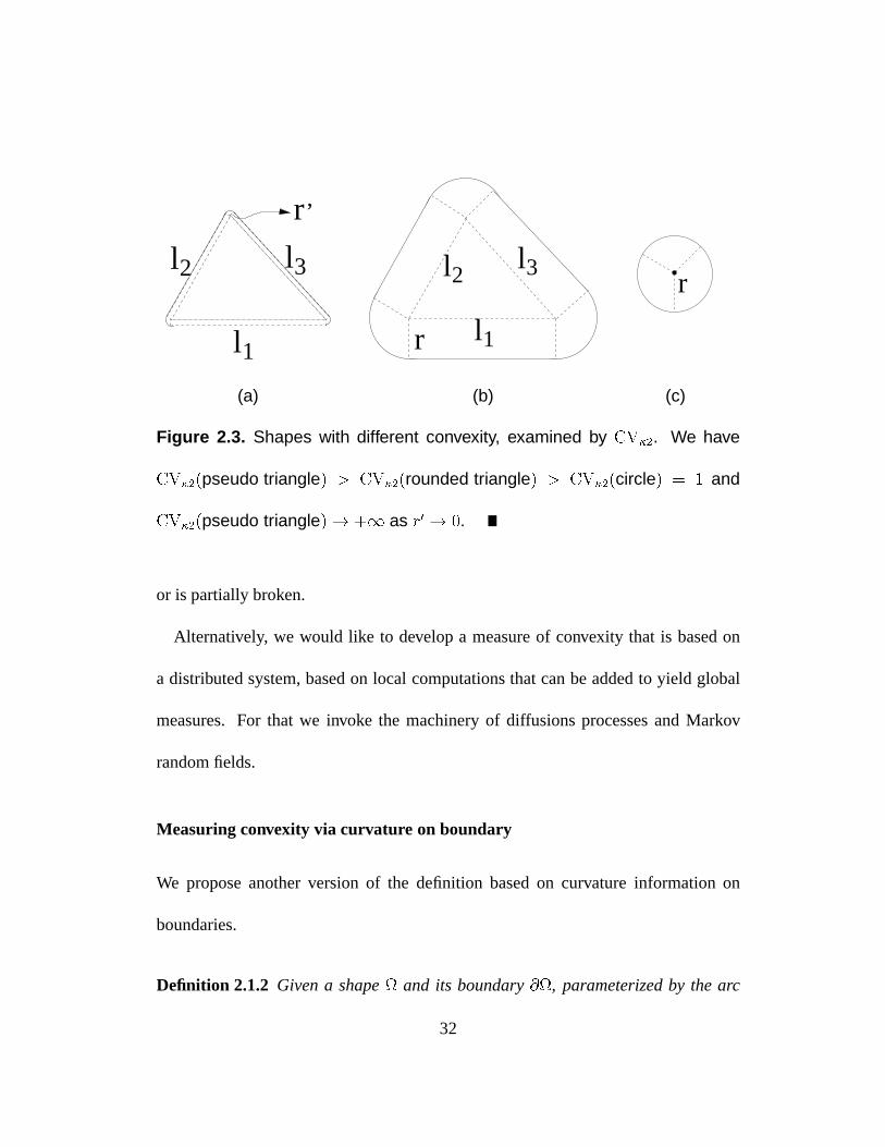
2.3 Shapes with different convexity, examined byCV2 . . . . . . . . . 32
xvii

2.4 Shape compactness measure is not appropriate in vision applications 35
2.5 Convexity measurement and decay effect introduced by . . . . . . 44
2.6 Continuous manner of decay convexity measure . . .. . . . . . . . 46
2.7 F/G separation by decay process: convexity and size preferences . . 47
2.8 Exponential decay in decay diffusion process. . . . . . . . . . . . 50
3.1 Decay convexity measure cannot give consistent prediction for trans-
lating convexity-versus-symmetry images . .. . . . . . . . . . . . 54
3.2 Concave cusp feature serves as cue for F/G .. . . . . . . . . . . . 57
3.3 Concave cusp feature as cue for F/G, caught by orientation process . 57
3.4 Orientation diffusion process and its boundary condition . . . . . . 62
3.5 Results of orientation diffusion process by two presentations . . . . 70
3.6 Arc image measured by orientation process . . . . . . . . . . . . . 72
3.7 The colonnade images of different sizes, measured by orientation dif-
fusion process . . . . . . . . . . . . . . . . . . . . . . . . . . . . . 76
3.8 Orientation process is more capable of picking concave cusp feature
than decay process. . . . . . . . . . . . . . . . . . . . . . . . . . 77
3.9 Convexity-versus-symmetry images of different sizes, measured by
decay process and orientation process . . . .. . . . . . . . . . . . 78
xviii

3.10 Level sets and relative entropy of ellipse and bell shapes, measured
by different’s . . . . . . . . . . . . . . . . . . . . . . . . . . . . 79
3.11 Convexity comparison between a concave shape and a circle, by de-
cay diffusion process . . . . . . . . . . . . . . . . . . . . . . . . . 80
3.12 Comparison between shapes with different sizes and convexity . . . 85
3.13 A square is favored over a rectangle . . . . .. . . . . . . . . . . . 87
3.14 The preference of triangle, hexagon and circle from decay process
and orientation proess . . . . . . . . . . . . . . . . . . . . . . . . . 89
3.15 Level sets of relative entropy for shapes with different convexity in
fine and coarse scales . . . . . . . . . . . . . . . . . . . . . . . . . 91
3.16 Level sets from decay process for shapes with different convexity in
various scales . . . . . . . . . . . . . . . . . . . . . . . . . . . . . 91
3.17 Convexity measure for various shapes with different convexity in dif-
ferent scales . . . .. . . . . . . . . . . . . . . . . . . . . . . . . . 92
4.1 Shape axis picked in the surfaceS with its characteristic points . . . 96
4.2 Shape axis is smoother than the symmetry axis . . . . . . . . . . . 97
4.3 Shape axis from decay process by-surface traveling method . . . 100
4.4 Most sinkage indicates the place of symmetry . . . . . . . . . . . . 104
xix

4.5 Shape axissym by choosing the resultant vector from result of
orientation process . . . . . . . . . . . . . . . . . . . . . . . . . . 106
4.6 Shape axissymM by choosing the maximum vectorM from result
of orientation process . . . . . . . . . . . . . . . . . . . . . . . . . 106
4.7 Shape axis with a continuous manner . . . . .. . . . . . . . . . . . 107
4.8 Shape axis with protrusion on boundaries and their transitions . . . 108
4.9 Junction informationjunc from orientation process . . . . . . . . . 109
4.10 Junction information as a global property of shapes .. . . . . . . . 110
5.1 Various illusory figures with different surface reconstructions . . . . 114
5.2 L-Junction with its various depth interpretations . . .. . . . . . . . 115
5.3 Kanizsa Square image with its optimal organization . . . . . . . . . 118
5.4 Kanizsa Square with different ratios ofr = R=L to decide . . . . 122
5.5 Four crosses image and its typical surface reconstruction . . . . . . 123
5.6 Four crosses image with its various organizations . .. . . . . . . . 124
5.7 Kanizsa square image with its various surface reconstructions . . . . 126
A.1 2-D Dirac-delta function defined on . . . . . . . . . . . . . . . . 135
B.1 Random walks in convex and concave regions. . . . . . . . . . . . 150
xx

List of Tables
1.1 The level of human tasks . . . . . . . . . . . . . . . . . . . . . . . 4
3.1 The convexity-versus-symmetry images measured by decay process
and orientation process with different’s . . . . . . . . . . . . . . 83
xxi

xxii

Chapter 1
Introduction
A goal in computer vision is to simulate human visual system with computer routines.
There are variations in the visual system among different individuals or even among
different occasions for the same individual. Thus, the general simulation must be de-
fined in a statistical sense. In general, the success of computer vision model is based
on some percentage of agreements between experiments in human visual system and
prediction of the computational simulation.
Statistics and Bayes Rule The performance of a visual system on a particular ex-
periment can be modeled as the outcome of a certain random variable. The random-
ness implies that, no outcome from any particular experiment will be essential as
testing data for our simulation. However, we pursue the general behavior for a group
1

of random variables. Two cases can be studied. When we try to build a theory across
different individuals, our principle is to search the agreement between the prediction
of our simulation and majority of outcomes from human tests. In this case, one “di-
verse” human visual system can be treated as an “imperfect machine”. More likely,
we accept a weaker, the computational view. The simulation is the goal to find a
model with the help of so-calledmethod of undetermined parameters, waiting for the
hidden parameters owned by each individual to be filled in.
On the other hand, we can also pursue the theory built for a single individual
among different occasions. When the outcomes are sorted by time,learning is in-
volved.
One basic rule applied in the decision making process is the Bayes Rule. Based on
an observation recorded by the vector x0, an objectA can be categorized as one of
k categoriesf!i; i = 1; :::; kg by investigating value of the conditional probabilityy
of !i onx0,
P (!ijx0) =p(x0j!i)P (!i)
p(x0); (1.1)
where
p(x0) =kXi=1
p(x0j!i)P (!i): (1.2)
A bold face will be used for vectors to distinguish from scalars.yWe use an upper-caseP to denote the probability mass function and a lower-casep to
denote the probability density function.
2
For a fixed observationx0, the result is decided by the conditional probabilityp(x0j!i)
and thea priori probabilityP (!i). Moreover, in the case whereP (!i) is a constant,
independent of the categories!i, we can adopt a more useful form,
P (!ijx0) / p(x0j!i) ; (1.3)
known as the maximum likelihood method. A larger conditional probabilityP (!ijx0),
called thea posterioriprobability suggests the decision “A belongs to the category
!i”. In the case where Eq. 1.3 can be assumed, we have a universal theory, indepen-
dent from the “time” and different individuals. When Eq. 1.3 is not applicable, for a
fixed individual, we look for an asymptotic result within a period, if there is any.
Let us discussP (!ijx0) for different applications. In high-level vision problems,
a decision may be made for guessing whether or not the object is a cat or a dog based
on some features in a given image. In low-level vision problems, the decision may
be the detection or not of a feature in a particular location of an image. Middle-
level vision makes the transition from a distributed (local) low-level information to a
more abstract, object oriented, perhaps symbolic representation. It may address the
problem of distinguishing between the figures and the background in images.
High-level x low-level vision In general, the concept of different level tasks in
human intelligence can be illustrated in Tab 1.1. The tasks in levelsn, n+1 andn+2
3

Level Task
...
n + 8 Tasting baptism water sweeter than normal water
n + 7 Knowing “Path Finder” may not find the path
n + 6 Realizing he is your grandfather if your father calls him father
n + 5 Ignoring the ads on the web
n + 4 Reading text through a mirror
n + 3 Object recognition
. . . . . . . . . . . . . . . . . . . . . . . . . . . . . . . . . . . . . . . . . . . . . . . . . . . . . . . . . . . . . . . . . . . . . .
n + 2 Object detection
n + 1 Texture detection
n Detection of intensity difference
...
Table 1.1. The level of human tasks. The tasks above the dot line may not be
accomplished by using only the visual system. The level n+ 5 and the levels
below it are called the literal levels.
4
may be accomplished by introducing only the visual system. The tasks in levelsn,
n+ 1 may be accomplished by applying only local considerations in images.
There are differences between low-level and high-level vision and we want to ex-
pand on this topic.
i In low-level vision many of the random variables, each associated with an im-
age feature, are defined everywhere in the image. In higher level vision, the
variables are more global (not defined everywhere in the image) and possibly
there are fewer variables than for the low-level vision case. Therefore, a vari-
able in the high-level vision is expected to have higher complexity than the
one in the low-level vision. It can lead to tough challenge for the high-level
simulation.
ii The distributions associated with low-level tasks are more ambiguous than for
high-level ones. One is expected to have, in general, more difficulties in decid-
ing whether there is a corner or not in an image location than to decide if there
is a face of a person in an image location. The distribution associated with face
recognition consists of so many different random variables (distributions) that
it is expected to be a much sharper/more peaked distribution (see Fig. 1.1).
iii There are more variations across human visual systems over the task-distributions
in the high-level vision than in the low-level vision. Someone that has never
5

seen birds will have a very different high-level description/distribution of a
bird when seeing one, than most of us who have seen birds. High-level de-
scriptions/distributions are learned through experience and therefore have more
varieties according to individual experiences. In this way, it is easier to collect
consistent data for a low-level human task than for a high-level one.
iv The outcome from the high-level task usually overrides the outcome from the
low-level task when there is a conflict. If an edge-boundary is needed to com-
plete a face figure the high-level system will “see” the edge, even if no intensity
gradient exists.
v The high-level task will interact more strongly with other brain activities (other
types of intelligence), such as in speech or upon playing chess.
From low-level to high-level, figure-ground separation and visual organization
The middle-level vision is where the transition from low-level vision to high-level
vision occurs. It transforms a distributed (local) set of informations into a coherent,
object oriented, abstract, description of the world, but yet, without naming objects or
recognizing objects from past experience (memory). In our view, it is where local
properties are integrated into surfaces or objects. The choice of intergration is called
visual organization.
6
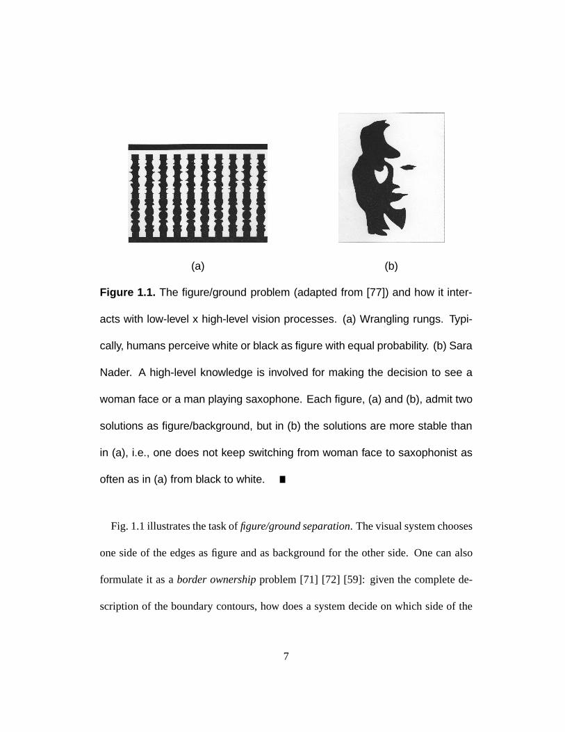
(a) (b)
Figure 1.1. The figure/ground problem (adapted from [77]) and how it inter-
acts with low-level x high-level vision processes. (a) Wrangling rungs. Typi-
cally, humans perceive white or black as figure with equal probability. (b) Sara
Nader. A high-level knowledge is involved for making the decision to see a
woman face or a man playing saxophone. Each figure, (a) and (b), admit two
solutions as figure/background, but in (b) the solutions are more stable than
in (a), i.e., one does not keep switching from woman face to saxophonist as
often as in (a) from black to white.
Fig. 1.1 illustrates the task offigure/ground separation. The visual system chooses
one side of the edges as figure and as background for the other side. One can also
formulate it as aborder ownershipproblem [71] [72] [59]: given the complete de-
scription of the boundary contours, how does a system decide on which side of the
7
boundary is the surface that gives rise to that border? It is the simplest visual organi-
zation problem where the search of organization is equivalent to the binary selection
of F/G. As formulated by the border ownership problem, usually, we discuss the F/G
separation through pairs of experiments of inverse intensities, as in the convexity-
versus-symmetry images in Fig. 1.6(a1) & (a2). Without the contrast polarity, the
result of F/G is decided by geometry of the (partial) shapes. To describe the F/G
problem by Bayes Rule, we can assume a constanta priori probabilityP (!i) with
!i = gure; ground in Eq. 1.1.
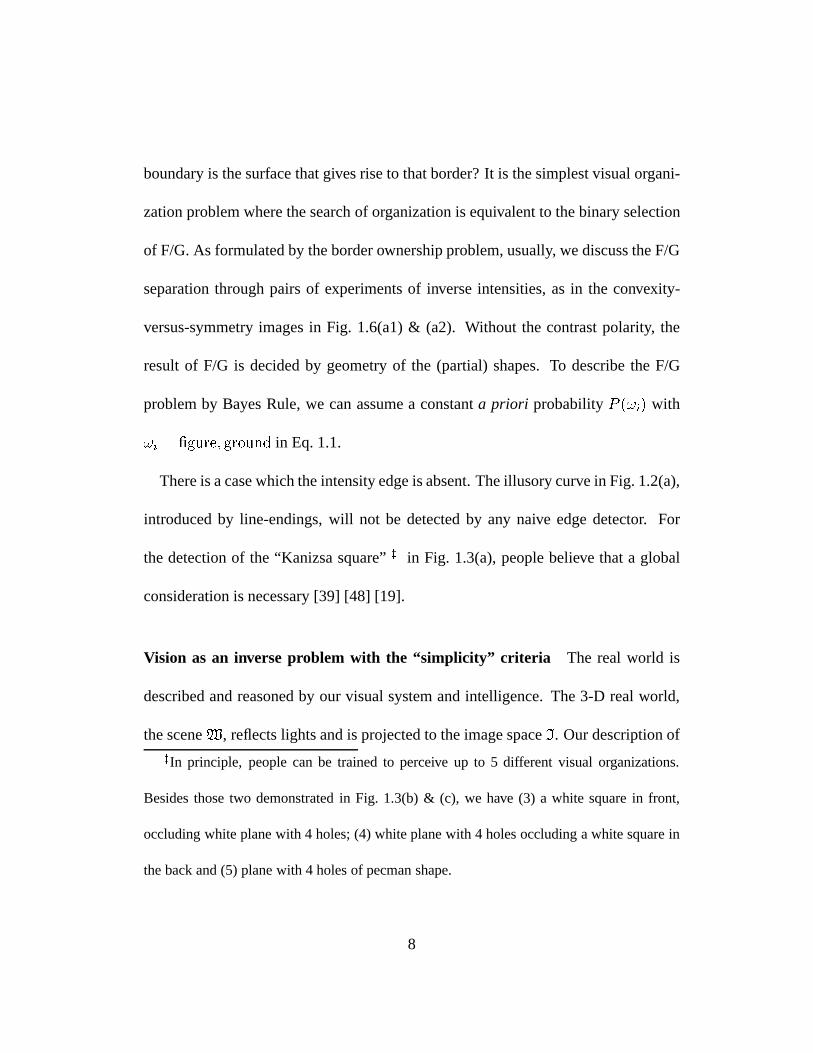
There is a case which the intensity edge is absent. The illusory curve in Fig. 1.2(a),
introduced by line-endings, will not be detected by any naive edge detector. For
the detection of the “Kanizsa square”z in Fig. 1.3(a), people believe that a global
consideration is necessary [39] [48] [19].
Vision as an inverse problem with the “simplicity” criteria The real world is
described and reasoned by our visual system and intelligence. The 3-D real world,
the sceneW, reflects lights and is projected to the image spaceI. Our description ofzIn principle, people can be trained to perceive up to 5 different visual organizations.
Besides those two demonstrated in Fig. 1.3(b) & (c), we have (3) a white square in front,
occluding white plane with 4 holes; (4) white plane with 4 holes occluding a white square in
the back and (5) plane with 4 holes of pecman shape.
8
(a) (b) (c)
Figure 1.2. (a) The illusory curve (adapted from Schumann [79]). (b) Random
oriented dots with the suggestion of closure. (c) Constant intensity square
with 1-D linear gray from 100% black to 100% white in the background from
left to right, inspired by Shapley and Gordon [76]. The illusory gradient is
perceived inside the square without any support of intensity changes. In par-
ticular, the gradient is extended in the direction perpendicular to the square
boundaries.
the scene is an inverse process from the image to the scene.
Wf I :
We consider searching of the inverse off , the mappingI 7!W, to be the computer
vision research. Given a single image, the mappingWf7! I is considered not 1-
1. It is neither an onto mapping in the sense that the majority part ofI is with low
probability within the range off . Most images in the image space are just white
9
(a) (b) (c)
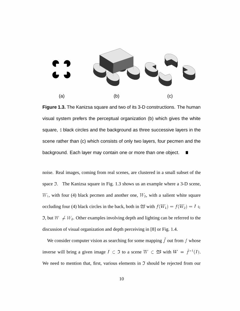
Figure 1.3. The Kanizsa square and two of its 3-D constructions. The human
visual system prefers the perceptual organization (b) which gives the white
square, 4 black circles and the background as three successive layers in the
scene rather than (c) which consists of only two layers, four pecmen and the
background. Each layer may contain one or more than one object.
noise. Real images, coming from real scenes, are clustered in a small subset of the
spaceI. The Kanizsa square in Fig. 1.3 shows us an example where a 3-D scene,
W1, with four (4) black pecmen and another one,W2, with a salient white square
occluding four (4) black circles in the back, both inW with f(W1) = f(W2) = I 2
I, butW1 6= W2. Other examples involving depth and lighting can be referred to the
discussion of visual organization and depth perceiving in [8] or Fig. 1.4.
We consider computer vision as searching for some mapping~f out fromf whose
inverse will bring a given imageI 2 I to a sceneW 2 W with W = ~f1(I).
We need to mention that, first, various elements inI should be rejected from our
10
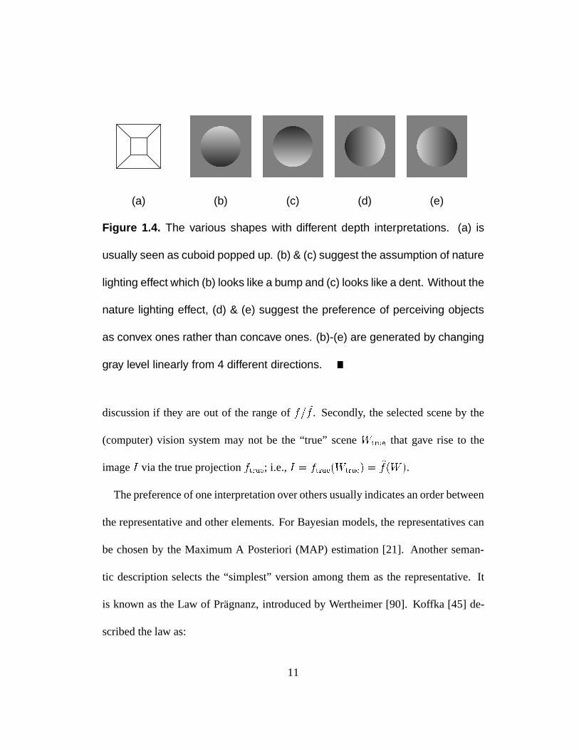
(a) (b) (c) (d) (e)
Figure 1.4. The various shapes with different depth interpretations. (a) is
usually seen as cuboid popped up. (b) & (c) suggest the assumption of nature
lighting effect which (b) looks like a bump and (c) looks like a dent. Without the
nature lighting effect, (d) & (e) suggest the preference of perceiving objects
as convex ones rather than concave ones. (b)-(e) are generated by changing
gray level linearly from 4 different directions.
discussion if they are out of the range off= ~f . Secondly, the selected scene by the
(computer) vision system may not be the “true” sceneWtrue that gave rise to the
imageI via the true projectionftrue; i.e.,I = ftrue(Wtrue) = ~f(W ).
The preference of one interpretation over others usually indicates an order between
the representative and other elements. For Bayesian models, the representatives can
be chosen by the Maximum A Posteriori (MAP) estimation [21]. Another seman-
tic description selects the “simplest” version among them as the representative. It
is known as the Law of Pr¨agnanz, introduced by Wertheimer [90]. Koffka [45] de-
scribed the law as:
11
Of several geometrically possible organizations that one will actually occur
which possesses the best, simplest and most stable shape.
For the Kanizsa square, the law can be expressed by having less corners to account
for the square/4-circle interpretation than the 4-pecman one. In noisy images, a more
regular geometry is easier to describe as it costs less information (in a compression
sense) and so one produces methods of image restoration to identify the “simplest”
image representative of the noisy image.
For the search of the function~f , it is possible that the search is exponentially hard
on the size of the images which one wants to explain. The so-called “visual orga-
nization research” is introduced to describe the physical or semantic structure from
the 2-D input. Operationally, this information dramatically reduces the number of
combinatorial alignments needed for searching possible figures in the scene, from
exponential to polynomial [25]. The evidences of experiments on human visual sys-
tems imply that the “depth”x information is appropriate for such mission [56].
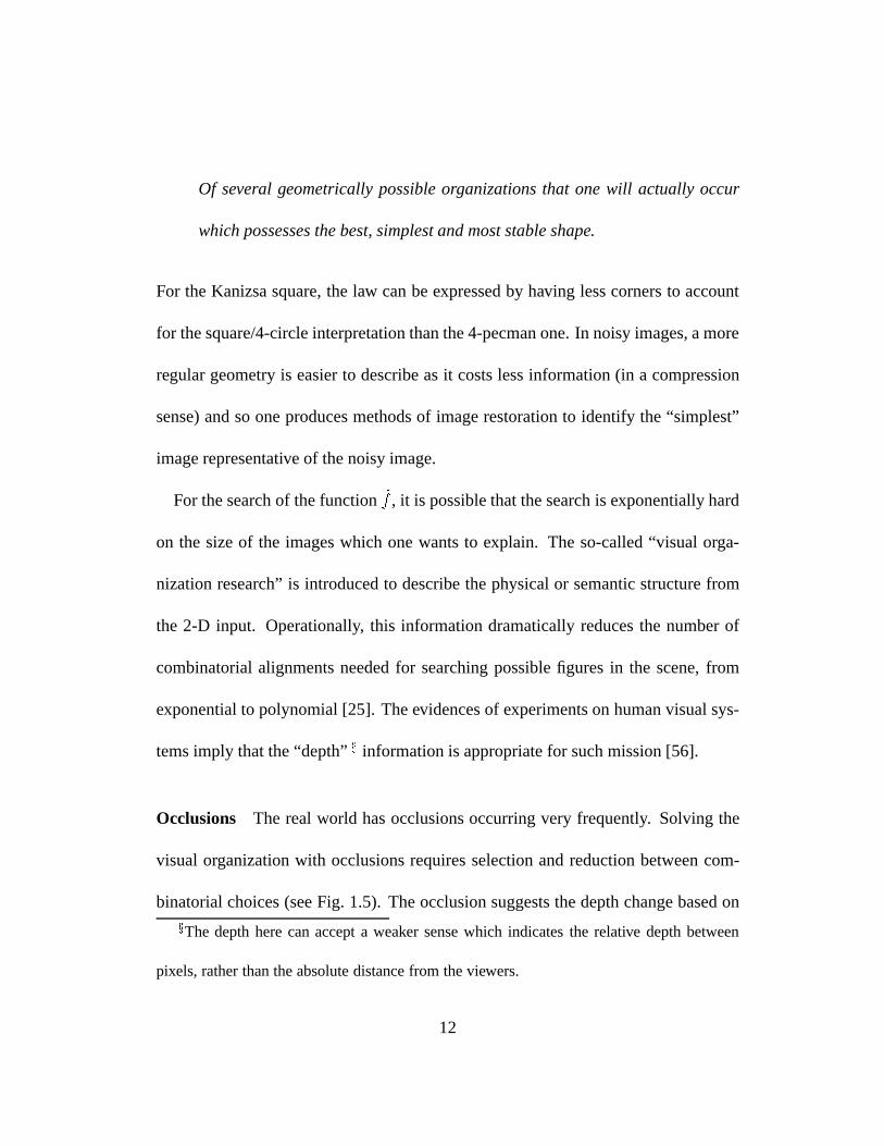
Occlusions The real world has occlusions occurring very frequently. Solving the
visual organization with occlusions requires selection and reduction between com-
binatorial choices (see Fig. 1.5). The occlusion suggests the depth change based onxThe depth here can accept a weaker sense which indicates the relative depth between
pixels, rather than the absolute distance from the viewers.
12
A
B
C
(a) (b) (c) (d) (e)
Figure 1.5. Various samples may introduce combinatorial explosion in the
identification process(adapted from Cooper [10]). (a) square identification,
and various objects violating the assumption of “flat objects” in 212-D recon-
struction, from simple to difficult: (b) nonrigid, (c) broken, (d) self-occluded
and (e) self-occluded with cycles.
local interpretations. In the Kanizsa square image, and various examples in Fig. 1.6,
the line endings, T- (or L-) junctions, convexity, size or parallelism suggest informa-
tion beyond 2-D [39] [48] [63] [32] [8] [56] [92] [79]. These are local cues in images,
an additional step from local to global is necessary [48] [86] [27].
Some past works are stated here. Kumaran et al. [48] approached the organization
problem from considering the local (corner) configurations. To conquer the input
with discretization, a perfect corner detector was assumed, same as the assumption
made in Mumford [58] and Williams and Jacobs [91] for the occluded edge comple-
tion by Elastica, with the assumption of “good continuation” for edges. Also, all of
their works showed no intention of handling different scales of images. The work of
13
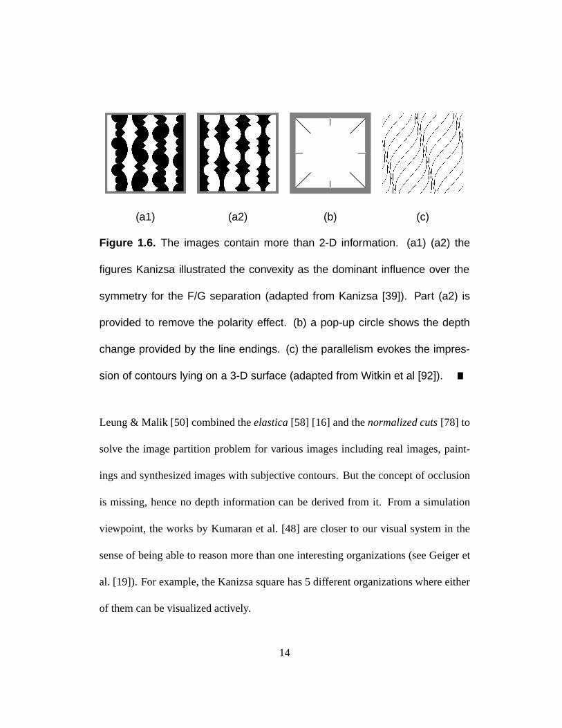
(a1) (a2) (b) (c)
Figure 1.6. The images contain more than 2-D information. (a1) (a2) the
figures Kanizsa illustrated the convexity as the dominant influence over the
symmetry for the F/G separation (adapted from Kanizsa [39]). Part (a2) is
provided to remove the polarity effect. (b) a pop-up circle shows the depth
change provided by the line endings. (c) the parallelism evokes the impres-
sion of contours lying on a 3-D surface (adapted from Witkin et al [92]).
Leung & Malik [50] combined theelastica[58] [16] and thenormalized cuts[78] to
solve the image partition problem for various images including real images, paint-
ings and synthesized images with subjective contours. But the concept of occlusion
is missing, hence no depth information can be derived from it. From a simulation
viewpoint, the works by Kumaran et al. [48] are closer to our visual system in the
sense of being able to reason more than one interesting organizations (see Geiger et
al. [19]). For example, the Kanizsa square has 5 different organizations where either
of them can be visualized actively.
14
Visual Organization, Figure/Ground, Shapes and Gestalt Laws We will consult
the Gestalt Laws [45] [46] [90] [8] for 2-D shapes and visual organization to sketch
the plan for salient figure selection. The Gestalt psychology is usually known by the
assertion “the whole is greater than the sum of its parts”. As we argued, the F/G
separation is the simplest example for the search of visual organization. It is the case
where the search of organization is equivalent to the binary selection from several
regions, which is also equivalent to investigation of the shape geometry. It is the
place where the Gestalt laws will be invoked.
The Gestalt laws says that proximity, convexity, similarity, good continuation, clo-
sure, relative size, surroundedness, orientation, symmetry are useful for F/G separa-
tion or visual organization construction [45] [46] [90] [8]. Our plan is first, construct
a model to quantify the Gestalt Laws for 2-D shapes and the quantified result will be
used in shape representations and evaluations. The salient surface is chosen based on
such information. In other words, we will design the shape representation with those
Gestalt laws included explicitly or implicitly.
1.1 Representation of Shapes
Our ultimate goal is to account for the Gestalt Laws of proximity (Ch. 2, 3), convexity
(Ch. 2, 3), good continuation (Ch. 5), closure (Ch. 5), relative size (Ch. 3), surround-
15
C2
C1
(a) (b1) (b2) (b3)
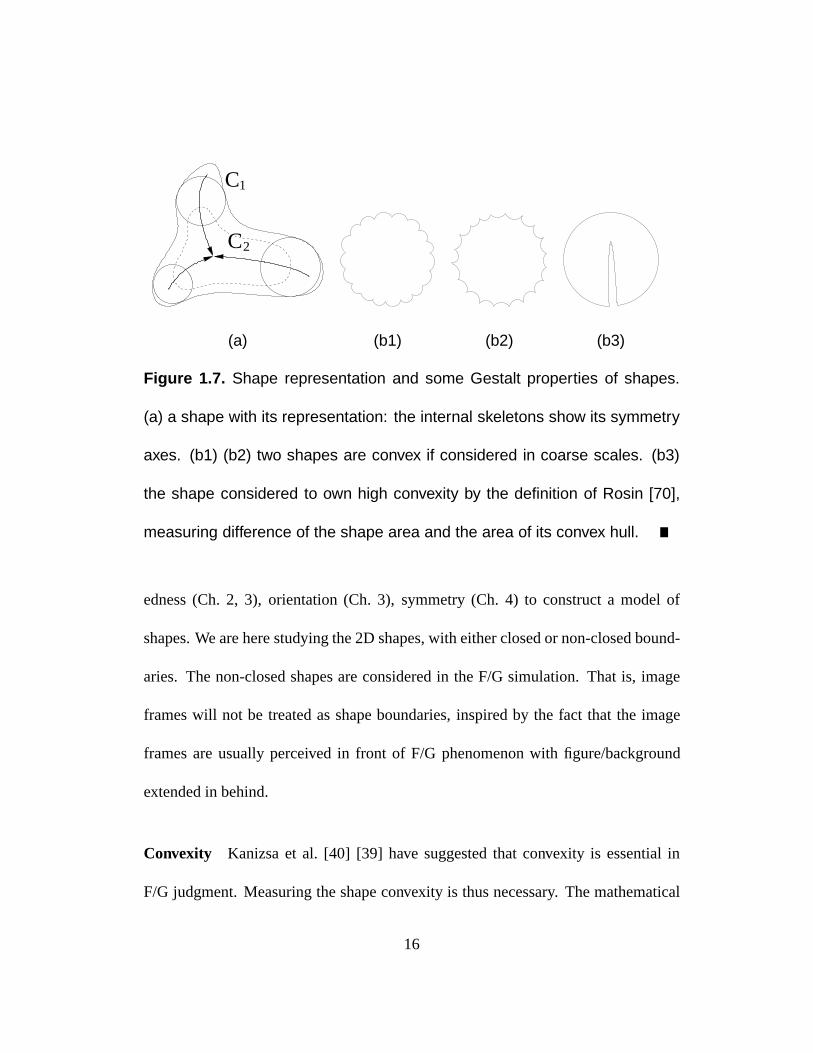
Figure 1.7. Shape representation and some Gestalt properties of shapes.
(a) a shape with its representation: the internal skeletons show its symmetry
axes. (b1) (b2) two shapes are convex if considered in coarse scales. (b3)
the shape considered to own high convexity by the definition of Rosin [70],
measuring difference of the shape area and the area of its convex hull.
edness (Ch. 2, 3), orientation (Ch. 3), symmetry (Ch. 4) to construct a model of
shapes. We are here studying the 2D shapes, with either closed or non-closed bound-
aries. The non-closed shapes are considered in the F/G simulation. That is, image
frames will not be treated as shape boundaries, inspired by the fact that the image
frames are usually perceived in front of F/G phenomenon with figure/background
extended in behind.
Convexity Kanizsa et al. [40] [39] have suggested that convexity is essential in
F/G judgment. Measuring the shape convexity is thus necessary. The mathematical
16
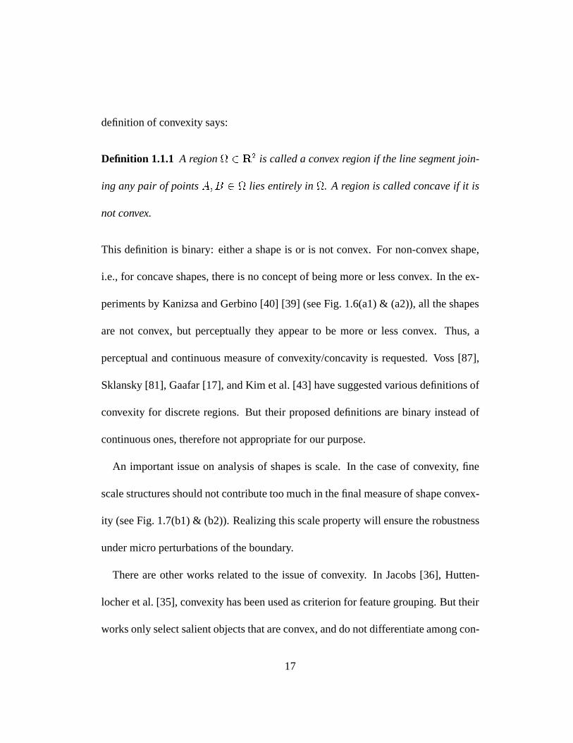
definition of convexity says:
Definition 1.1.1 A region 2 R2 is called a convex region if the line segment join-
ing any pair of pointsA;B 2 lies entirely in. A region is called concave if it is
not convex.
This definition is binary: either a shape is or is not convex. For non-convex shape,
i.e., for concave shapes, there is no concept of being more or less convex. In the ex-
periments by Kanizsa and Gerbino [40] [39] (see Fig. 1.6(a1) & (a2)), all the shapes
are not convex, but perceptually they appear to be more or less convex. Thus, a
perceptual and continuous measure of convexity/concavity is requested. Voss [87],
Sklansky [81], Gaafar [17], and Kim et al. [43] have suggested various definitions of
convexity for discrete regions. But their proposed definitions are binary instead of
continuous ones, therefore not appropriate for our purpose.
An important issue on analysis of shapes is scale. In the case of convexity, fine
scale structures should not contribute too much in the final measure of shape convex-
ity (see Fig. 1.7(b1) & (b2)). Realizing this scale property will ensure the robustness
under micro perturbations of the boundary.
There are other works related to the issue of convexity. In Jacobs [36], Hutten-
locher et al. [35], convexity has been used as criterion for feature grouping. But their
works only select salient objects that are convex, and do not differentiate among con-
17

cave or convex shapes in a continuous manner. In Weiss [89], convexity was used as
the criterion for F/G separation without considering the small-size preference for F/G
(see next paragraph). Besides, the regional consideration was left out. All of their
works can not account, nor aim to do so, for the Kanizsa and Gerbino experiments.
Also, the concept of scale was missing in those approaches. Results can be altered
by fine-scale perturbations.
In the research of shape analysis, various definitions of convexity was proposed for
shape decomposition. One approach is to examine the difference between a shape
and its convex hull. For instance, Rosin [70] used the area difference between the
shape and its convex hull to define a continuous convexity. In Held et al. [29], a
continuous measure of convexity, calledapproximate convexitywas defined based
on the fraction of region boundary coinciding with convex hull of the region. In
many cases, shape attributes like area and perimeter are not enough to specify the
shape properties. For the shape in Fig. 1.7(b3), the area difference between the shape
and its convex hull is small, therefore, own a high convexity by the definition of
Rosin [70]. We claim that missing of the internal axis information is the key for the
failure. The shape in Fig. 1.7(b2) will obtain a bad convexity measure in the sense of
approximate convexity by Held et al. [29].
18
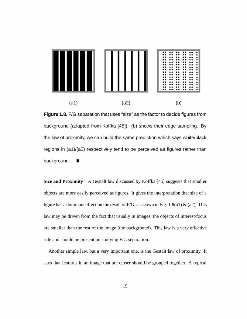
(a1) (a2) (b)
Figure 1.8. F/G separation that uses “size” as the factor to decide figures from
background (adapted from Koffka [45]). (b) shows their edge sampling. By
the law of proximity, we can build the same prediction which says white/black
regions in (a1)/(a2) respectively tend to be perceived as figures rather than
background.
Size and Proximity A Gestalt law discussed by Koffka [45] suggests that smaller
objects are more easily perceived as figures. It gives the interpretation that size of a
figure has a dominant effect on the result of F/G, as shown in Fig. 1.8(a1) & (a2). This
law may be driven from the fact that usually in images, the objects of interest/focus
are smaller than the rest of the image (the background). This law is a very effective
rule and should be present on studying F/G separation.
Another simple law, but a very important one, is the Gestalt law of proximity. It
says that features in an image that are closer should be grouped together. A typical
19
image example is given with set of black dots in white background and perceptually
the closer ones are grouped together.
We can relate these two laws by the following argument. Suppose we have smaller
objects in an image, once features such as edges are extracted, they will be grouped
by the proximity law. The border ownership problem will then be resolved. I.e.,
edges that belong to larger objects will give the ownership to smaller objects since
the latter ones will be grouped together. Then smaller objects become salient/figures.
One can see this effect in Fig. 1.8(b). Once the edges are extracted and grouped by
proximity, they will belong to the smaller width strips, and so smaller width strips
will be figures and the larger width strips will be the background.
Symmetry Axis and Symmetry Measure The symmetry axis was first introduced
by Blum [4] as thegrass firedescription. For a given curveC0(s) parametrized by
s, Kimia et al. [44] [80] extended the idea of Blum by giving a nice description of
shape and medial axis via the evolution equation
@tC = (0 1) ~N ;
C(s; 0) = C0(s) :
with ~N denotes the normal vectors in boundaries. The coefficients0 and1 were
used to produce the constant flow and the curvature flow respectively. The medial
20
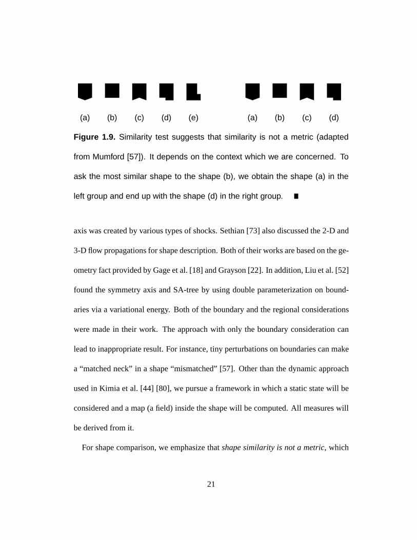
(a) (b) (c) (d) (e) (a) (b) (c) (d)
Figure 1.9. Similarity test suggests that similarity is not a metric (adapted
from Mumford [57]). It depends on the context which we are concerned. To
ask the most similar shape to the shape (b), we obtain the shape (a) in the
left group and end up with the shape (d) in the right group.
axis was created by various types of shocks. Sethian [73] also discussed the 2-D and
3-D flow propagations for shape description. Both of their works are based on the ge-
ometry fact provided by Gage et al. [18] and Grayson [22]. In addition, Liu et al. [52]
found the symmetry axis and SA-tree by using double parameterization on bound-
aries via a variational energy. Both of the boundary and the regional considerations
were made in their work. The approach with only the boundary consideration can
lead to inappropriate result. For instance, tiny perturbations on boundaries can make
a “matched neck” in a shape “mismatched” [57]. Other than the dynamic approach
used in Kimia et al. [44] [80], we pursue a framework in which a static state will be
considered and a map (a field) inside the shape will be computed. All measures will
be derived from it.
For shape comparison, we emphasize thatshape similarity is not a metric, which
21

was discussed in Mumford [57]. First, the matching process between shapes is not
symmetric. If we sayA is similar toB, what we mean isB is some kind of prototype
in a category which includesA. Also, the similarity betweenA andB depends
strongly on contexts. E.g., in Fig. 1.9, by given a shape, we are asked to choose the
most similar one among others. In the experiment I(the left group), we are asked
the most similar one tob among others. In the experiment II(the right group),e is
removed and the same question is asked again. Many people reported thata is the
most similar one tob in the experiments I whiled is the most similar one tob in the
experiment II. It gives
d(b; a) < d(b; c); d(b; d); d(b; e) and d(b; d) < d(b; a); d(b; c) :
A contradiction occurs. Therefore, to search for a universal concept of shape simi-
larity is not appropriate.
1.1.1 A Continuous Simulation
We consider the shape representation from a brand-new approach. We call it the
continuous simulation.
For the convexity measure, instead of using the binary definition adopted in mathe-Suppose there is a non-symmetric metric “d” and d(x; y) denotes the difference for “x
compared toy” (not vice versa).
22
matics, we would like to search for a continuous version definition. By this definition,
we can discuss “more convex” shapes and “less convex” shapes, for two non-convex
ones. Our comparison will be meaningful even between two perfectly convex shapes.
For study of the symmetry axis, we would like to derive a new axis representation
of shapes. On this representation, more than giving the information telling a point is
on or off an axis, we would like to provide the information which can describe “how
likely” a point is on the axis or “how strong” this axis is.
We will also provide a way to detect junction features. For the junction detection,
we look for a representation which instead of giving a brutely1 or 0 declaration, will
provide the transition from low-curvature curves, high-curvature curves to curves
with discontinuous curvature.
1.1.2 A Global Simulation
In our simulation, we consider the shape information as a whole. For convexity
measurement, we would like to have the ability to discuss the coarse scale convexity.
For the symmetry axis, the information which we look for is based on a global
consideration. So a small axis coming from noise in fine scales shall not be confused
with main axes of the shape.
For the junction detection, we will not only concentrate on the finest scale fea-
23

tures. We are also able to pick up junction features in coarse scales, with a stronger
declaration.
1.2 Problem Proposed
For a given single and still image, my proposed problems are
i How can we characterize 2D shapes via local computations and diffusion pro-
cesses where this characterization is particular useful in perceptual simulation?
ii How can the Gestalt studies help us in defining such shape characterization ?
iii How can we find one (or more than one) plausible organization(s) from an
image based on the study of 2-D shapes ?
For the first two topics, in Chapter 2 and Chapter 3, two models will be proposed,
called thedecay diffusion processand theorientation diffusion processso as two
measures called thedecay diffusion measureand theorientation diffusion measure.
The F/G separation and shape convexity will be discussed through these two mea-
sures. In Chapter 4, we use two ways, from the results of the decay process and the
orientation diffusion process to generate the shape axis. Also, junction information
can be derived from the result of orientation process. For the third topic, in Chapter 2
and 3, we use the result from shape analysis to predict the F/G. In Chapter 5, we
24

discuss salient shape selection and visual organization. We conclude our result and
sketch the future work in Chapter 6.
25

26
Chapter 2
Convexity and Size in Figure/Ground
Separation
2.1 From Binary to Continuous Definitions
For a (compact) shape and its boundary set@, we discuss the idea of convexity.
In mathematics, convexity is described by
tP1 + (1 t)P2 2 : 8t 2 [0; 1]; P1&P2 2 (2.1)
The condition of the definition can be changed to an equivalent one as8t 2 [0; 1],
8P1&P2 2 @, checking only boundary points. Sometimes, only part of or @ is
visible due to restriction of image frame. E.g., in Fig. 2.2, onlya is visible out of
27
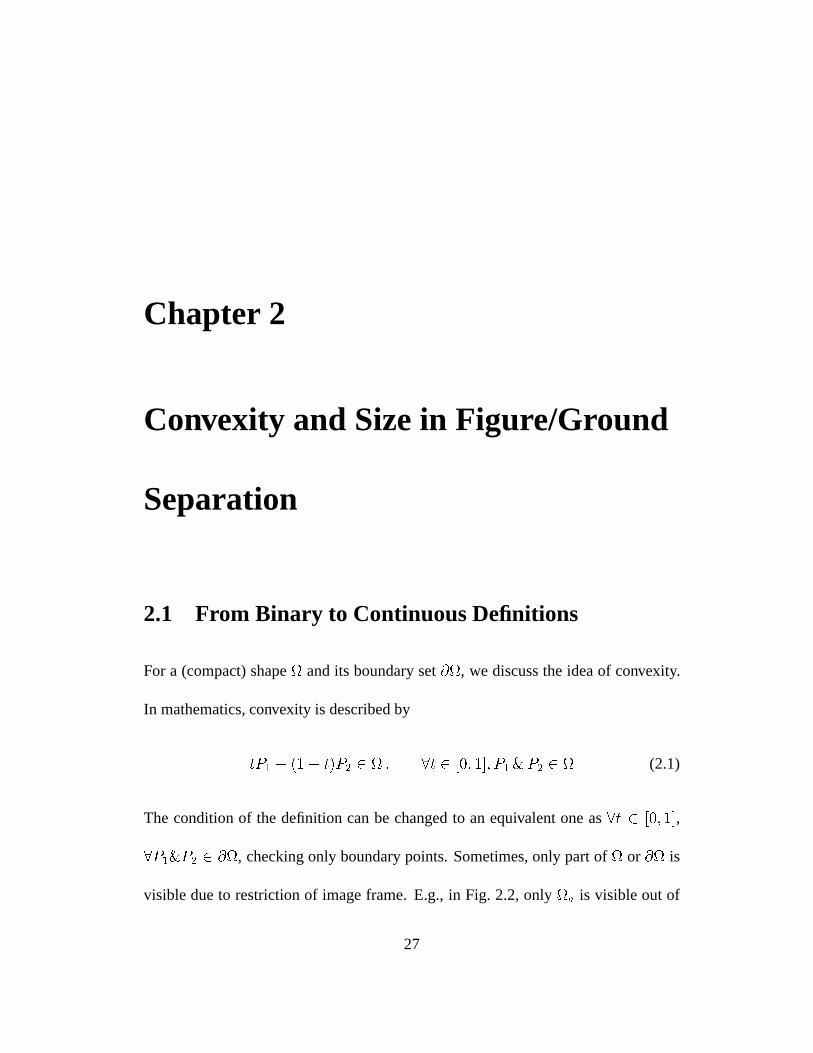
(a) (b)
Figure 2.1. The figures adapted from Kanizsa et al. [39] [40] to illustrate
the important role of convexity in F/G separation. Human results show the
black/white area in (a)/(b) respectively is more likely to be considered as fig-
ures.
a complete region with its partially visible boundary curves @. A definition
similar to Eq. 2.1 can be formulated for the partial cases such as the regiona or its
partial boundary. The equivalence argument between checking boundary points or
interior points can also be made.
The idea of convexity for F/G separation was proposed by Kanizsa et al. [39] [40]
in their convexity versus symmetry experiments. In Fig. 1.6(a1) & (a2) and Fig. 2.1,
the idea of “convexity” (other than symmetry) is proposed as the dominant criteria
for F/G decision. However, the convexity of these regions does not follow the mathe-
matical definition of convexity in the sense that most regions are considered concave.
Therefore we need a continuous version definition for convexity which allows us to
distinguish between “more” and “less” convex shapes. Various definitions will be
discussed.
28
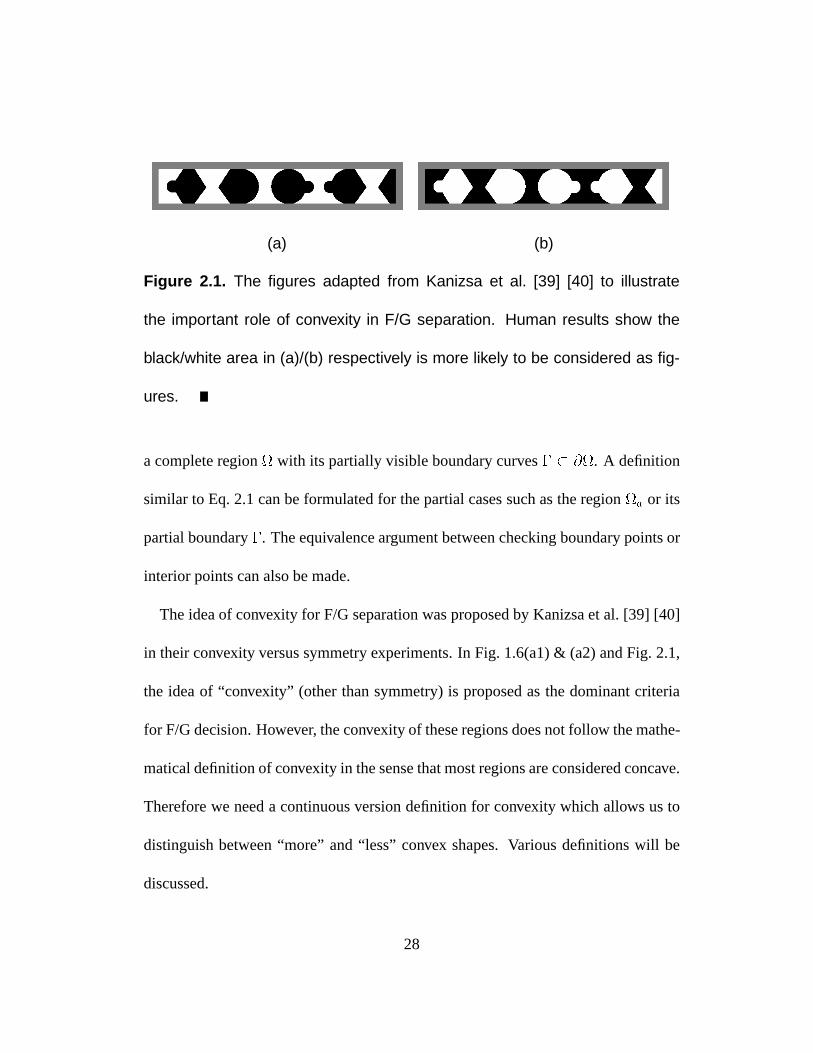
Ω
V−convexity
−convexityU
−Ω
B
A
2
P3
P4
1 Ω
2
P1
ΩQ
Q
ab P
Γ
(a)
Figure 2.2. The convexity examination of the region and its complement
sitting on two sides of the boundary @. The regions , and boundary
@ may be only partially explored and end up with a, b and respectively.
We measure convexity by shortest paths connecting two points through two
(partial) regions a and b separately.
Measuring convexity via shortest path
Let us analyze Fig. 2.2 and try to propose a continuous measure of convexity. We
have a rectangular frame, an imageI, divided into two regionsa andb I a,
both with the same area (within the frame) and a common edge boundary. Before
we can decide the border ownership problem, we assume a and b. Both
regions, if interpreted as shapes, are concave and yet, we perceive one region as more
29
convex than the other.
We observe that in Fig. 2.2(a), length of the segmentP1P2 a is shorter than
length of the curve]P1P2 b. For pointsP3 andP4, the straight segmentP3P4 a
connects two points in the convex side, but a longer path, the segmentsP3Q2 [
Q2P4 b is chosen in the concave side. The smaller the angle\Q2 is, the bigger
the difference between the length of the two shortest paths (s.p.) in both regions.
The same is true for the case where (the integral of) curvature in the curve]P1P2 gets
larger. In Fig. 2.2(a), based on the evidence pointsP1 andP4, the regiona is more
convex than the regionb by owning the shorter pathP1P3P4 a compared to the
pathP1Q1Q2P4 b.
We then propose a definition of convexity as follow. The version which we will
give is for a complete shape. A similar version for partial exploreda, b or can
also be formulated similarly.
Definition 2.1.1 Given a shape and its boundary@, we estimate the shortest
pathsp(Pi; Pj) between pair of pointsPi; Pj wheresp(Pi; Pj) & Pi; Pj2@. Its
length is denoted byEsp(Pi; Pj). Suppose@ is parameterized by its arc length, we
define s.p. convexityas the integral of such distance over all pairs of points on@,
CVsp1(@) =
Z L
0
Z L
0
Esp(P (s1); P (s2)) ds1 ds2 ; (2.2)
whereL is length of@. It can be normalized by the Euclidean distancekP (s1)
30
P (s2)k, which gives
CVsp2(@) =
Z L
0
Z L
0
Esp(P (s1); P (s2)) ds1 ds2Z L
0
Z L
0
kP (s1) P (s2)k ds1 ds2
: (2.3)
A rough estimation gives
CVsp1(@) ML2 ;
whereM denotes the maximum lengthEsp for pair of points in@. For a per-
fectly convex shape, M is its diameter. For the normalized version, we have
CVsp2(@) = 1 for convex shapes, andCVsp2(@) > 1 for concave shapes. It
provides a continuous definition of convexity. On the other hand, we can write a
variant of the definition which checks all points in instead of@. We can also
consider the case when image frame exists. We compare convexity for two (partially
explored) regionsa andb with a shared edge by computing convexity of them
via either the boundary or the regional version of the definition.
Let us take a look at these measures. Suppose we sample@ by N points, the
computation of these measures requiresO(N2) operations and it can not be paral-
lelized belowO(N) computations. One needs to verify, for each pointP (s(i)), all
the other pointsP (s(j))0s. Moreover, it assumes that the shape is given. I.e., it does
not provide an automatic way to extend this approach when shapes need to be de-
tected, e.g., the case of noisy images or illusory figures where the shape is not clear
31
’
2l
r
1l
3l
r
l2
l
l
1
3r
(a) (b) (c)
Figure 2.3. Shapes with different convexity, examined by CV2. We have
CV2(pseudo triangle) > CV2(rounded triangle) > CV2(circle) = 1 and
CV2(pseudo triangle)! +1 as r0 ! 0.
or is partially broken.
Alternatively, we would like to develop a measure of convexity that is based on
a distributed system, based on local computations that can be added to yield global
measures. For that we invoke the machinery of diffusions processes and Markov
random fields.
Measuring convexity via curvature on boundary
We propose another version of the definition based on curvature information on
boundaries.
Definition 2.1.2 Given a shape and its boundary@, parameterized by the arc
32
lengths. The curvature convexityis given by
CV1(@) =1
2
Z L
0
j(s)j ds; (2.4)
where denotes curve curvature on@. Or we can try a quadratic form
CV2(@) =L
42
Z L
0
j(s)j2 ds: (2.5)
For shapes with smooth boundary, we haveCV1(@) = 1 for any convex shapes
andCV1(@) > 1 for concave shapes. For non-smooth boundaries where some
undefined curvature points were occurred, we can make them “curved” and compute
the convexity on the perturbed ones. It will be well-defined. It gives us
CV1(circle) = CV1(triangle) = 1 :
The second definitionCV2 can only be discussed on smooth curves. For a circle of
arbitrary radius, we haveCV2(circle) = 1. In fact,CV2 is invariant under scaling.
For figures in Fig. 2.3, we have
CV2(pseudo triangle) > CV2(rounded triangle) > CV2(circle) = 1 :
A similar one calledaverage bending energy, normalized by the curve length instead,
was given byE(@) = 1L
R L0 j(s)j2 ds in Young et al. [93]. Our definition is made to be
size-invariant.
33
The computation givesCV2(rounded triangle) = 1+(l1+ l2+ l3)=2r. So we have
CV2(rounded triangle)! +1 if r! 0
CV2(rounded triangle)! 1 if l1 + l2 + l3 ! 0 :
In fact, Young et al. [93] proved that circle shape will minimize the criteria, either
the curvature convexityCV2 or their average bending energy, if the curve length is
fixed. It is possible to have a convex shape owning bigger measure ofCV2 than a
concave shape.
Let us check how effective these measures are. First of all, both definitions are not
appropriate in the F/G problem, either for measuring convexity of complete regions
& or incomplete regionsa & b with shared edges on an image (Fig. 1.6(a1)
& (a2) and Fig. 2.1). Those regions will have the exact same value on both sides no
matter what we consider, the smoothed or non-smoothed versions. Again, we need to
know the shape before we can execute the computation involved in both definitions.
Compactness
We discuss a related criteria calledshape compactnessy, which has been discussed in
Bacus et al. [2], Green [23], Rosenfeld [69] and Bribiesca [7].yIn Young et al. [93], the average bending energy, similar to the convexity definitionCV2
was used to substitute the conventional definition of shape compactness.
34
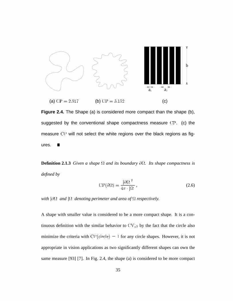
1 a2a
b
(a) CP = 2:917 (b) CP = 3:152 (c)
Figure 2.4. The Shape (a) is considered more compact than the shape (b),
suggested by the conventional shape compactness measure CP. (c) the
measure CP will not select the white regions over the black regions as fig-
ures.
Definition 2.1.3 Given a shape and its boundary@. Its shape compactness is
defined by
CP(@) =j@j2
4 jj; (2.6)
with j@j andjj denoting perimeter and area of respectively.
A shape with smaller value is considered to be a more compact shape. It is a con-
tinuous definition with the similar behavior toCV2 by the fact that the circle also
minimize the criteria withCP(circle) = 1 for any circle shapes. However, it is not
appropriate in vision applications as two significantly different shapes can own the
same measure [93] [7]. In Fig. 2.4, the shape (a) is considered to be more compact
35
than the shape (b), if measured byCP. To apply this measure to F/G simulation,
it will not give a correct prediction. For example, we can design a F/G experiment
such as in Fig. 2.5(a) where both regions own the same area. It gives the same
compactness for both regions if only the edge boundaries are considered as shape
boundaries. If we do consider the image frame as part of the shape boundaries, we
will not select the white regions in Fig. 2.4(c) as the favored regions. Their mea-
sures areCPwhite = 4(a1 + b)2=(4a1b) andCPblack = 4(a2 + b)2=(4a2b). It gives
CPwhite > CPblack if b2 > a1a2 or b > a1; a2, which is the case in Fig. 2.4(c).
Namely, for this size/proximity experiment, we will collect a result against the per-
ceptual phenomenon, predicting black regions as figures. In fact, the area term is
assigned as the denominator. Therefore, larger regions will be favored given the
same perimeter. To accomplish the task of F/G separation, a measure with the
small-size preference is preferred, if a measure with size preference is offered. On
the other hand, the convexity definitionCVsp1, given by examining shortest paths
within shapes, is more appropriate than the shape compactnessCP, for deciding
F/G. Smaller shapes will be favored, with shorter shortest-paths.
U-convexity andV-convexity
Let us discuss two different types of convexity. In Fig. 2.2, the regionA andB
are considered different as on boundaries of the regionA (an arc or aU), curvature
36
= _(s) (suppose orientation is parameterized by the arc lengths) shares the same
sign while boundaries ofB (an angle or aV) has curvature equal to0 except at the
angle peak. The first kind is called arc convexityor U-convexityand the second
kind is called angle convexityor V-convexity. We say that the convexity is concen-
trated on a single point on the boundaries withV-convexity (regionB) while it is
more uniformly distributed over the boundaries withU-convexity (regionA). It tells
one important difference between them. When a small aperture is randomly put on
these two kinds of boundaries, we have a better chance of knowing where the convex
side is by putting it on the boundaries withU-convexity than the boundaries withV-
convexity. We argue that this local suggestion makes theU-convexity more favorable
than theV-convexity. Another evidence of our argument comes from the experiments
provided by Stevens et al. [82] or Fig. 3.2. The concave cusp feature (more like own-
ing V-convexity) suggests that it is the background side rather than the figures. Also,
in the Kanizsa image in Fig. 1.6(a1), we do have similar number ofU’s (arcs) or
V’s (angles) for the black and white regions. Although, the perception provides the
preference of black regions (with moreU-convexity) as figures.
In the next section and in Chapter 3, we proceed to construct two kinds of convex-
ity measure. Thedecay diffusion measureis derived by a process called thedecay
diffusion processand theorientation diffusion measureis from a process working on
the domain ofI [0; 2), called theorientation diffusion process. They are the 1st
37
and 2nd order of Markov processes respectively. Those images and perceptual ex-
periments that we have discussed will be studied again under these measures. As we
have discussed, the measures that we will propose is based on a distributed system,
a highly-parallelizable algorithm. Besides, the frameworks should not be recognized
as having only the goal to derive the (convexity) measures for F/G prediction. Other
features of shapes, such as symmetry or junctions, can also be obtained as side re-
sults. It will be discussed in Chapter 4.
2.2 Decay Diffusion Process
We seek a computational model to measure convexity of a complete or partial shape
or a in a continuous manner. Based on boundary input, the first step of our
framework is designed to generate a field insidez the shape while the value of each
point can be viewed as convexity on that point. The field calleddecay diffusion field
is derived by a leaking energy diffusion process where the discrete formulation can
link this process to a 2-D decay walk, starting from the boundaries (Appendix B). It
means that the computation during this part can be done locally through interactions
between adjacent pixels. A judgment of convexity, called convexity measure is givenzThe inside (or outside) means just one side of an closed contour, depending on where the
interesting part is. For a partial shape, the interesting region is restricted within the image.
38
by computing (point-wise) entropy of the field belonging to. A shape with a smaller
measure is called a more convex shape. More discussions will show that not only
convexity, but also size preference, will be caught by this measure. As we know,
both are important to F/G. From now on, we will not clearly distinguish a complete
shape from a partial onea or @ from unless it is necessary to do so. We use
and@ throughout our formulation.
2.2.1 Decay Diffusion Process as Energy Minimization
Notations and Assumptions
Given a binary synthesized imageI [0; A] [0; B] R2 with the characteristic
functionI(x) of the region as intensity function. The feature set of the image, is
given by the edge/boundary set@ = fx 2 I : 9Nx s:t: I(x) 6= I(Nx)gwhereNx
is drawn from the neighborhood set of the pointx. A discretization in the Euclidean
grid gives four neighbors asNx = f(x1+1; x2); (x11; x2); (x1; x21); (x1; x2+1)g
for the pointx = (x1; x2). We record this edge set by its characteristic functione(x),
which is,
e(x) =
8>><>>:
1 ; if x 2 @
0 : if x 2 @
(2.7)
Rest of the formulation is set related to this function (as well as the intensity function
39
I). The input0, also called the inducer or hypothesis function, is given by
0(x) =
8>><>>:
1 ; if x 2 @
0 : if x 2 @
(2.8)
The area of is recorded byjj, andj@j denotes length of the edge set.
Variational Formulation
We adopt a variational formulation in our framework. Solving of the decay diffusion
field is the minimization process on a given energy. The energy functional which we
are interested in is
Edecay(j0;; ) =
Z
(x) ((x) 0(x))2 +M(x) kr(x)k2 dx ; (2.9)
for a given input0. The function : ! R is the field we need to evaluate. The
function(x) in the first term (data fitting) is given by
(x) =
8>><>>:
Æ2(x) ; if x 2 @
; if x 2 @
(2.10)
whereÆ2(x) stands for the 2-D Dirac delta function s.t.R@Æ2(x) dx = 1. A com-
plete definition can be found in Appendix A. In the discrete case, it is provided by
(x) = 1=;x 2 @ for a small constant, called the delta function coefficient(Ap-
pendix B). On the inside part of, we choose(x) = , a small positive constant
called the decay coefficient. The functionM(x) in the second term (smoothness),
40
called smoothness function is simply assigned asM(x) = 1 for the homogeneous
case.
The first part stands for fidelity to the input. The second part stands for the smooth-
ness assumption, minimizing square of the gradient valuekr(x)k. Let us re-
organize the energy functional into two parts @ and@ and write down its
Euler-Lagrange equation
(x) = (x) ; x 2 @
(x) = 0(x) ; x 2 @
(2.11)
where = @xx + @yy is the Laplacian operator. When touches image frame, an
absorbing barrieris assumed for the boundary condition.
We solve the equation by the finite difference method which will be demonstrated
in Appendix B. The solution, written as(x) is the decay diffusion field we need.
Practically, for the convexity comparison of two shared-edge regions within an im-
age, we solve the field for both regions andI simultaneously by discretely
assigning0 = 1 and1 to both sides of the edges. As for the original image
Fig. 2.5(a), we assign black/white color as1=1 to pixels on both sides of the edges,
and assign50% gray or0 to pixels inI@ representing0(x), so called the inducers
or the hypothesis function. A simple example of F/G image is shown in Fig. 2.5.
41
2.2.2 Entropy Criteria
In order to obtain a convexity measure, first, we convertx the field1 (x) 1
into a probability distribution at each pixel, via a linear mapping
p(x) =1
2(1 + (x)) : (2.12)
For a F/G problem,p(x) can be treated as the probability of being in front (salient).
In Appendix B, we will give a random walk formulation to describe the solution
as well as the probability fieldp. As we will show in Appendix B,p(x) is the
probability to reach any “figure inducers” before reach any “background inducers”,
for a walk starting atx. Either with or without broken edges, the probability to reach
“background inducers” can be greater than zero. The reason is that the walks stopped
in interior points will be considered having half of the probability contributing to
the “background part”, as it lacks of knowledge to commit. Therefore, it is natural
to characterize the region as the setfx : p(x) 0:5g andI as the setfx :
p(x) < 0:5g. When two regions on both sides of edges are solved simutaneously, the
(discrete) pixels on the edges, wherep(x) = 1=0 (or (x) = 1= 1) is considered
as the strongest commitment to be salient/background respectively. The place withxIt is possible to have(x) 0 as we are solving the field simultaneously on both sides
of the edges. Later when we introduce the mechanism of organization selection for illusory
figures, we have another case of(x) 0. Please see Chapter 5 for more discussion.
42

p(x) = 0:5 (or (x) = 0) stands for the place being neutral or non-commitant.
The criteria is given by calculating (point-wise) entropy of the shape,
S(p) = 1
jj
Z
p(x) log p(x) + (1 p(x)) log(1 p(x)) dx : (2.13)
A shape withsmallermeasureS is considered more convex. As we said, we can
substitute the sub-index of the summation by an equivalent conditionp(x) 0:5. We
compute this measure for both regions andI, indicated byS andS respectively.
Conventionally,p(x) = 1=0 is reserved for convex/concave side respectively and we
useS to denote the measure for convex side andS for concave side if the convex or
concave side can be easily distinguished. The sharper the diffusion, the closer to1=0
p(x) for / I is, the smaller the entropy we can obtain. The entropy is a point-
wise entropy or entropy of the region normalized by the area of in the discrete
case.
2.2.3 Convexity and Decay Coefficient
We analyze our model by the random walk formulation. In Appendix B, a discrete
form energy functional will be given and the process becomes a decay walk in 2-D.
From the random walk viewpoint, the solution(x) is the summation of probability
carried by all the walks starting from inducers on boundaries (may be with different
weights) to the pixelx. The decay coefficient controls how strong the decay effect
43
200 250 300 350
50
100
150
200
250
(a) (b) (c) (d)
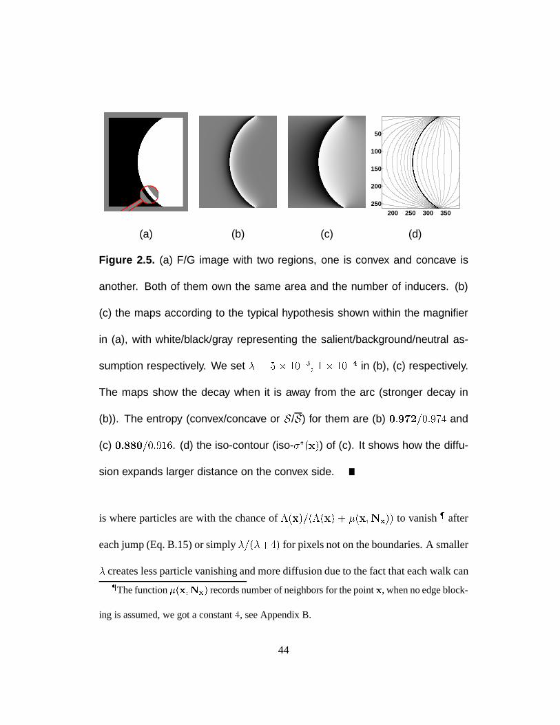
Figure 2.5. (a) F/G image with two regions, one is convex and concave is
another. Both of them own the same area and the number of inducers. (b)
(c) the maps according to the typical hypothesis shown within the magnifier
in (a), with white/black/gray representing the salient/background/neutral as-
sumption respectively. We set = 5 103; 1 104 in (b), (c) respectively.
The maps show the decay when it is away from the arc (stronger decay in
(b)). The entropy (convex/concave or S/S) for them are (b) 0:972=0:974 and
(c) 0:880=0:916. (d) the iso-contour (iso-(x)) of (c). It shows how the diffu-
sion expands larger distance on the convex side.
is where particles are with the chance of(x)=((x) + (x;Nx)) to vanish after
each jump (Eq. B.15) or simply=(+4) for pixels not on the boundaries. A smaller
creates less particle vanishing and more diffusion due to the fact that each walk canThe function(x;Nx) records number of neighbors for the pointx, when no edge block-
ing is assumed, we got a constant4, see Appendix B.
44
remain for a longer period. The effect is illustrated in Fig. 2.5(b) and (c). The idea
why convexity is caught by our model can be presented in the following way. First
of all, random walks tend not to cross over boundaries. The chance of particles
vanishing on boundaries is given by1=(1 + (x;Nx)) with a small. So we can
assume that the walks are more likely to visit the boundaries only once by choosing a
small enough. Therefore, we can discuss walks in the convex side and the concave
side separately. For walks starting from boundary inducers to points in or I ,
shorter ones in the convex side will be accumulated which mean less decay while
longer ones will be chosen in the concave side (see Fig. B.1). In Fig. 2.5(d), it can be
seen that the convex side has wider iso-contour than the concave side, which means
a sharper diffusion and a smaller convexity measure.
Continuous Convexity Measure
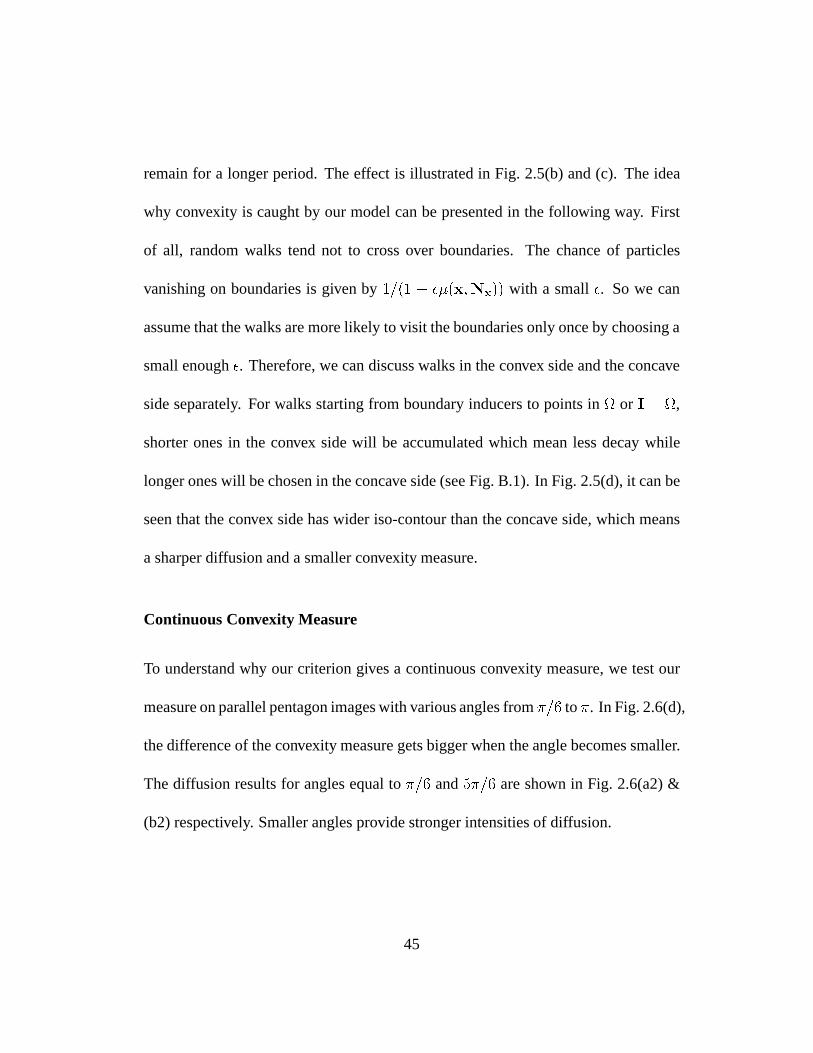
To understand why our criterion gives a continuous convexity measure, we test our
measure on parallel pentagon images with various angles from=6 to. In Fig. 2.6(d),
the difference of the convexity measure gets bigger when the angle becomes smaller.
The diffusion results for angles equal to=6 and5=6 are shown in Fig. 2.6(a2) &
(b2) respectively. Smaller angles provide stronger intensities of diffusion.
45
(a1) (a2)
(b1) (b2)
50 100 150 200 250
20
40
60
(c)
20 40 60 80 100 120 140 160 1800
0.02
0.04
0.06
0.08
0.1
0.12
0.14
Degree of Angle
Ent
ropy
(bac
kgro
und)
− E
ntro
py(f
oreg
roun
d)
Convexity vs Entropy Difference
(d)
Figure 2.6. (a1) (b1) source images with angles of =6 and 5=6 and (a2)
(b2) their diffusion result (only middle parts are shown). The entropy val-
ues for (a2) and (b2) are 0:721 / 0:870 (convex/concave or S / S) and 0:944 /
0:950 respectively, with = 1 104. (c) The iso-contour with angle equal to
=2 (complete map). (d) The difference between entropy for the convex and
concave regions as a function of the angle (“inverse of convexity”).
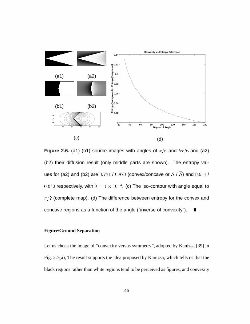
Figure/Ground Separation
Let us check the image of “convexity versus symmetry”, adopted by Kanizsa [39] in
Fig. 2.7(a), The result supports the idea proposed by Kanizsa, which tells us that the
black regions rather than white regions tend to be perceived as figures, and convexity
46
(a) Original (a) Diffusion (c) Original
(b) Original
(b) Diffusion (c) Diffusion
Figure 2.7. F/G separation by the decay process, with the convexity and size
preferences. (a) the Kanizsa figure for the convexity-versus-symmetry ex-
periments. The entropy values are S=S = 0:546=0:560 for the black/white
regions respectively. Beware that we have more diffusion near the neck area.
(b) another F/G dominated by the figural convexity. The decay measure gives
the measure as S=S = 0:723=0:747, favoring the “shell” shapes, the white re-
gions. (c) The size preference is given by the measure of S=S = 0:220=0:602,
favoring the white/small strips.
47
is the key for this phenomenon. Another example given in Fig. 2.7(b), prefers the
“shell” shapes. We discuss other properties of our model in the following sections.
2.2.4 Size and Proximity
As we mentioned, the idea of using size as a criteria for F/G separation is highly
related to the Gestalt law of proximity. In our model, as we can realize in the random
walk argument that proximity between the inducers of a shape and any points in
the shape is the key for large intensities of diffusion. So for the size preference
test in Fig. 2.7(c), without any effect of convexity, our model will prefer the white
regions which are the regions with smaller size. This is because the white regions
have inducers closer to each other, where inducers will support the diffusion in the
nearby regions before the particles vanish in an exponential decay. An extreme case
can be given by neglecting the smoothing in Eq. 2.9. We have(x) = 0(x). The
convexity measure is given by
S(p) =jj j@j
jj= 1
j@j
jj: (2.14)
A smaller area (or more number of inducers) will yield a smaller measure. It matches
our visual perception, a known fact proposed by Koffka [45].
48
Size Invariance and Tuning of
We would also like to discuss the relation betweensimilar shapes with different sizes.
It can be seen from the Euler-Lagrange equation in Eq. 2.11. In Eq. 2.11, for a scaling
of s from the shape to0, we subsititutex by x0 = sx and let0(x0) = (x), also
00(x0) = 0(x). A new equation is obtained as
s20(x0) = 0(x0) ; x0 2 0 @0
0(x0) = 00(x0) : x0 2 @0
(2.15)
It means that if we choose a new decay coefficient0 = =s2, we can collect a similar
field 0 to the original field with 0(x0) = (x).
To speak of the convexity measure, we consider Eq. 2.13. For two probability maps
p andq with p(x) = q(x0) derived from and0 on and0 respectively, we
have
S(q) =1
j0j
Z0q log q + (1 q) log(1 q) dx0
=1
s2jj s2Z
p log p + (1 p) log(1 p) dx = S(p) : (2.16)
Therefore, the same convexity measure can be obtained for both shapes if the decay
coefficient is carefully adjusted.
49
RΩΟ
0 50 100 150 200 2500
0.1
0.2
0.3
0.4
0.5
0.6
0.7
0.8
0.9
1Profile of a Circle
Location
Fie
ld
0 50 100 150 200 2500
0.1
0.2
0.3
0.4
0.5
0.6
0.7
0.8
0.9
1Profile of a Circle
Location
Fie
ld
(a) (b1) (b2)
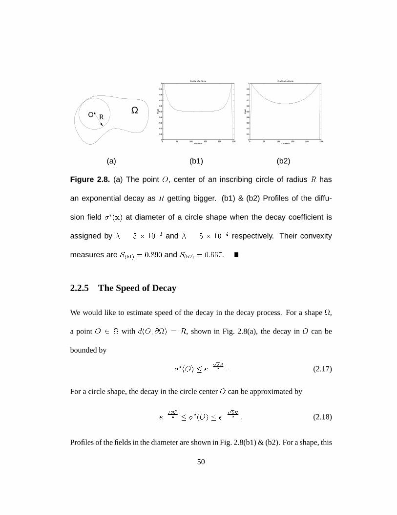
Figure 2.8. (a) The point O, center of an inscribing circle of radius R has
an exponential decay as R getting bigger. (b1) & (b2) Profiles of the diffu-
sion field (x) at diameter of a circle shape when the decay coefficient is
assigned by = 5 103 and = 5 104 respectively. Their convexity
measures are S(b1) = 0:890 and S(b2) = 0:667.
2.2.5 The Speed of Decay
We would like to estimate speed of the decay in the decay process. For a shape,
a pointO 2 with d(O; @) = R, shown in Fig. 2.8(a), the decay inO can be
bounded by
(O) epR2 : (2.17)
For a circle shape, the decay in the circle centerO can be approximated by
eR2
4 (O) epR2 : (2.18)
Profiles of the fields in the diameter are shown in Fig. 2.8(b1) & (b2). For a shape, this
50
exponential decay weakens the possible description of its coarse scale structures. For
“highly convex” shapes with minor perturbations such as the shapes in Fig. 1.7(b1)
& (b2), an appropriate convexity measure should depend on not only fine scale con-
vexity, but more importantly, coarse scale convexity. To improve this, in next chapter,
the orientation measure will be introduced based on the orientation diffusion process.
2.2.6 Implementations
We choose the parameter set as the decay coefficient = 5 103 and the delta
function coefficient = 101. This set is fixed throughout all our experiments unless
different notification is given.
For the F/G problem, we design the input images with the same size in both of
the black and white regions. By doing this, we remove the size bias which may be
created in Eq. 2.14. Also, we would like to discuss the boundary condition with more
details.
Boundary Condition
As we mentioned, all experiments are tested under the assumption of absorbing bar-
riers for image frames, which has(x) = 0 if x 2 @I. To be more careful, we can
choose the frame used for computation to be a little bigger than the image frame.
The principle is to choose a frame for computation big enough s.t. we can assume
51

all walks going beyond the (computation) frame are likely to be stopped. So those
walks can be ignored in computation without losing too much precision for the final
measurement. When the image frame is extended, in Eq. 2.13, we use the criteria of
fx :p(x) 0:5g=fx :p(x) < 0:5g to characterize figure/ground respectively.
In perception, this assignment is interpreted as the F/G phenomenon prevailing
below image frames with certain range. For an evidence, we can refer to Fig. 2.7(c)
where we can perceive a fatter strip near the boundaries in the right end.
52
Chapter 3
Orientation Diffusion Process
The purpose of quantifying convexity of shapes was inspired by figure/ground sepa-
ration. Therefore, a convexity measure was pursued and applied to F/G problems. We
consider this measure a definition of shape convexity, with the small-size preference.
With the perceptual evidences provided by Kanizsa [39], this definition is useful for
the F/G problems, by providing F/G predictions statistically similar to the results
from our visual systems. Computationally, our model was designed in a distributed
system; hence, a highly parallelizable scheme can easily be obtained. Let us dis-
cuss how well this decay diffusion model can fit our goals from different viewpoints.
Again, we do not try to distinguish between partial or complete shapes. Although
as a measure to suggest F/G it is more likely to discuss partial shapes, while as an
abstract definition for shape convexity, we are interested more in the complete ones.
53

(a1) (a2) (b2)
Figure 3.1. When we horizontally translate the boundaries in (a1), a copy of
Fig. 2.7(a1) to (a2), we have a different convexity judgment from the decay
model. The diffusion result of (a2) is in (b2) with the convexity measures
S=S = 0:588=0:515, predicting the white regions as figures, opposite to the
result for (a1) which gives S=S = 0:546=0:560, predicting the black regions
as figures. Nevertheless we did not perceive much difference between (a1)
& (a2) which has just pixels difference in location.
Figure/Ground Separation
From the F/G point of view, presumably, we can use the output from the decay model
to predict the answer of F/G. More precisely, based on the studies of the convexity
and size preferences of the decay measure in the last chapter, we should be able
to use the measure in F/G prediction if the F/G phenomenon in input images are
dominantly decided by these two factors. The remaining question is that, in the
54
decay model, we need to check if these two are “well-balanced/normalized” as in
our visual systems. We design a simple experiment by horizontally translating the
boundaries of the convexity-versus-symmetry image in Fig. 3.1. Under the convexity
shape preference which yields the preference of black regions in (a1) as figures, the
knowledge of small shape preference also tells us the following phenomenon:
When we translate the boundaries via the direction of expanding/shrinking the
black/white regions respectively, we can expect the white regions will eventually be-
come the prevailing parts as figures rather than background.
This phenomenon can be seen either through our model or the experiments in our
visual systems (e.g. Stevens et al. [82]). For each of them, a “no difference” point
exists where both regions share the same preference there. So the succeeding ques-
tion is: Will they happen to be identical to each other? From Fig. 3.1(a1) to (a2), we
horizontally translate the boundaries for a few pixel distance. The result from the de-
cay model shows the result ofS=S = 0:546=0:560 for (a1) andS=S = 0:588=0:515
for (a2). It suggests a “black region preference” in (a1) and a “white region prefer-
ence” in (a2), opposite to our perceptual observation where we can hardly describe
the difference between them if one of them is hidden from the other. Namely, our
model is too sensitive to the size preference. It indicates a failure and we would like
to improve it by accounting for this observation.
In the new framework as well as the new convexity measure that will be proposed,
55
a free parameter is provided and two no-difference points from the simulation and
our visual systems can be synchronized by tuning this parameter.
Definition of Convexity
In the decay model, a convexity measure favoring small size regions has been pro-
posed. If this measure is considered as a quantitative definition for shape convex-
ity, it is natural to ask for a size-invariant one. By adjusting the decay coefficient
(Eq. 2.9, 2.10), it is possible to give the same measure from the decay process for
similar shapes with different sizes, according to Eq. 2.15 and Eq. 2.16. But the choice
of needs region area as an input. In general, this knowledge is not available before
the whole shape outline is detected. So this adjustment is not preferable for images
containing illusory shapes, or noisy images. We would like to put it forward, with
more flexibility. We would like to construct a convexity measure with or without the
preference of small size regions.
In the next two sections, we will discuss some technical issues and see why the
decay diffusion model is not appropriate under such considerations.
U-convexity,V-convexity, Boundary Curvature and 2nd Order Transition
On boundaries, we examine two typical types of convexity, theV-convexity and the
U-convexity, defined in Sec.2.1 or Fig. 2.2. For the curves withV-convexity, the
56
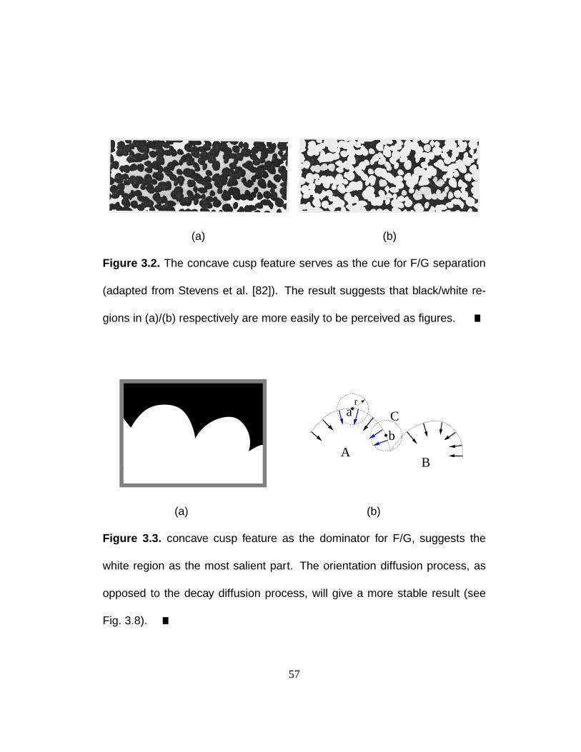
(a) (b)
Figure 3.2. The concave cusp feature serves as the cue for F/G separation
(adapted from Stevens et al. [82]). The result suggests that black/white re-
gions in (a)/(b) respectively are more easily to be perceived as figures.
B
C
Ab
ar
(a) (b)
Figure 3.3. concave cusp feature as the dominator for F/G, suggests the
white region as the most salient part. The orientation diffusion process, as
opposed to the decay diffusion process, will give a more stable result (see
Fig. 3.8).
57
convexity is concentrated on one peak of the boundaries, while for the ones with
U-convexity, the convexity is more uniformly distributed along the boundaries.
Perceptually, we say that theU-convexity is more preferred than theV-convexity.
As we argued in Sec. 2.1, if boundaries with both types are sampled through asmall
aperture, more likely, the F/G can be picked up from boundaries withU-convexity
than withV-convexity, for the reason that most areas (except the peak) inV-convexity
boundaries provide no clue for the F/G. For theU-convexity boundaries, F/G is more
likely to be decided in a small scope, and in a separated way. Namely, for theU-
convexity ones, we can decide the F/G by a small scope observation and by only
one of the numerous observations. It is important, for the reason that profiles pro-
jected from objects in the 3-D world are mostly partial, broken or occluded and more
collections of such local suggestions give a better chance to decide F/G efficiently.
Furthermore, the angle peaks/junctions inV-convexity regions sometime suggest a
potential visual organization movement. Different organization constructions lead to
different F/G choices and figural hypotheses can be assigned on either the convex
or concave side [48] [19] [32] [33] [34]. In various situations, junctions, the place
with theV-convexity, are produced by object overlapping seen through a particular
perspective, and hence, are of no physical significance. All these reasons show more
importance of theU-convexity than theV-convexity, and it may lead to the prefer-
ence of theU-convexity for F/G separation. It is true that information collected by
58
a small aperture is local, sometime incompatible with other local decisions and can
be altered by a global consideration in visual organization construction. However,
we discuss the boundaries with only the “balanced” presence ofU-convexity andV-
convexity. In this situation, the F/G decision will be chosen favoring theU-convexity
rather than theV-convexity. It is exact the case in the convexity-versus-symmetry
image provided by Kanizsa [39] (Fig. 1.6(a1), (a2) or Fig. 3.1) where number of
U-convexity andV-convexity curves are similar.
Another similar evidence is provided by Stevens et al. [82]. In Fig. 3.2, they argue
that the concave cusp feature is the dominator for F/G. We tend to choose black area
as figures in (a) or white area as figures in (b). For a concave cusp (more like owning
theV-convexity) in Fig. 3.3, the white region (owning theU-convexity) will be the
favored part.
To speak of the decay diffusion model, a discussion can be made in the concave
cusp in Fig. 3.3(b). We draw a small circle at either the pointa or b with the same
radiusr. For the diffusion result, we say that the pointb gets better support on the
black side than the pointa on the white side because the circle centered inb covers
more inducers than the circle centered ina. This fact may lead a better result in the
black region than in the white region. A numerical evidence is shown in Fig. 3.8.
We can consider curves with theU-convexity andV-convexity from a different
view. Suppose the diffusion from boundaries are set to be oriented, i.e., the bound-
59
ary inducers,0 in Eq. 2.8 or Eq. 2.9 are oriented ones, depending on the bound-
ary normals and delivered by an oriented transition (a tendency to keep the previ-
ous orientations). In the curves withU-convexity, we can see diffusion comes from
neighboring points and “converging” with similar orientations while for the curves
with V-convexity, we either have no such “convergence” or have “convergence” from
non-adjacent neighboring inducers. A 2nd-order Markov chain will be used as the
transition mechanism to carry those normal information to form a regional descrip-
tion of shapes.
We are interested in another experiment which may be related to the discussion in
this section. In Fig. 1.2(c), an image generated by a square with constant intensity and
1-D linear0100% gray on the background (inspired by Shapley et al. [76] where a
circle figure was used). The intensity difference on boundaries suggests the illusory
gradient inside the square, even no intensity change is provided. In particular, the
gradient is extended in the direction perpendicular to the square boundaries. We are
interested in what process can simulate this effect.
The Speed of Decay and Coarse Scale Structures
In Sec. 2.2.5, we estimated the speed of decay in the decay process. The decay is
exponential, therefore the field lose structures when it is far from inducers. For the
convexity measure, few structure in coarse scales will be considered. For convex
60

shapes with fine-scale perturbations, such as Fig. 1.7(b1) & (b2), an appropriate con-
vexity measure should depend on not only fine scale convexity, but more importantly,
coarse scale convexity.
3.1 Orientation Diffusion in R2 S
1
The new convexity measure based on an orientation diffusion process will be pro-
posed to improve the decay model in the following sense:
i. The new measure allows the flexibility of switching between measuring con-
vexity with or without size preference.
ii. The 2nd order Markov chain is used as the transition mechanism to simulate
the preference ofU-convexity overV-convexity.
iii. Fine scale protrusion, either convex or concave can only have minor contribu-
tion to the final measure.
iv. The measure can distinguish two perfectly convex shapes. The result shows a
simulation of the Law of Pr¨agnanz for 2-D shapes (described in Chapter 1 or
by Wertheimer [90] and Koffka [45]).
v. Many shape attributes, such as symmetry and junction feature can be naturally
obtained through computation of the measure.
61
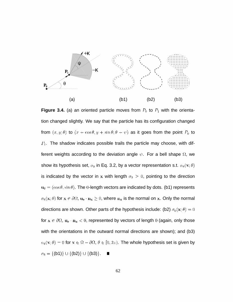
θ
ψ
0P
P1
+
−κ
κ
(a) (b1) (b2) (b3)
Figure 3.4. (a) an oriented particle moves from P0 to P1 with the orienta-
tion changed slightly. We say that the particle has its configuration changed
from (x; y; ) to (x + cos ; y + sin ; + ) as it goes from the point P0 to
P1. The shadow indicates possible trails the particle may choose, with dif-
ferent weights according to the deviation angle . For a bell shape , we
show its hypothesis set, 0 in Eq. 3.2, by a vector representation s.t. 0(x; )
is indicated by the vector in x with length 0 0, pointing to the direction
u = (cos ; sin ). The 0-length vectors are indicated by dots. (b1) represents
0(x; ) for x 2 @, u nx 0, where nx is the normal on x. Only the normal
directions are shown. Other parts of the hypothesis include: (b2) 0(x; ) = 0
for x 2 @, u nx < 0, represented by vectors of length 0 (again, only those
with the orientations in the outward normal directions are shown); and (b3)
0(x; ) = 0 for x 2 @, 2 [0; 2). The whole hypothesis set is given by
0 = f(b1)g [ f(b2)g [ f(b3)g.
62
We will discuss the first four topics in this chapter and postpone the fifth topic to the
next chapter.
The plan is designed similarly to the decay model. After a field is generated by
a process, we derive a measure by a point-wise computation. The new diffusion
process, called the orientation diffusion, augment the working space for diffusion
from the image spaceR2 toR2 S1 with an additional dimension [0; 2). The
idea of orientation diffusion can be illustrated in Fig. 3.4(a). Apart from the decay
diffusion which is considered as a random walk or a Brownian motionW (t) with the
property
The incrementW (t)W (s) is independent ofW (s) : 8t s
The walk carries no memory other than its location as it proceeds. The orientation
diffusion takes additional memory in the orientation dimension. With a known ori-
entation at times, it is more likely to keep this orientation to the next status of
time t, up to some noise. In Fig. 3.4(a), a particle with the configuration(x; y; )
at the times could end up with the next step of timet with a new configuration
(x + cos ; y + sin ; + ) where is created by noise. While the previous model
caught convexity by the support of two near points, we now catch convexity in a
different sense.The support of orientation diffusion is always from neighboring in-
ducers, unlike the support of decay diffusion which may come from two non-adjacent
63
ones. E.g., in the diffusion map in Fig. 2.7(a) & (b) or Fig. 3.1(b2), results generated
by the decay process, we can find more diffusion near the neck area of the white
regions.
Some works have been done with models dealing with oriented data or working on
an oriented space. Tang et al. [85] collected the unary oriented information as input
and a process, called thedirection diffusionwas applied to the data regularization.
Some other works related to image regularization and segmentation by isotropic or
anisotropic diffusion can be referred to Weickert [88]. Mumford [58], William and
Jacobs [91] used an oriented process and applied the EulerElasticaof two oriented
sources (junctions) to complete occluded-curves. Unlike those works, our works
are derived from boundary input, and the result is recorded by a vector-bundle field
instead of a scalar or a vector field. Besides, our interests are concentrated on de-
scribing 2-D shapes, including deriving convexity measure, computing shape axis
and junction information.
3.1.1 Variational Formulation and Energy Functional
Notations
For a given region (represented by its boundaries@) in an input imageI, either
partial or complete, we discuss its convexity. A set of useful information is collected
64
as follows. For an intensity functionI(x), the oriented edge map
e(x; ) =1
Me
@I(x)@u
2 [0; 1]; x 2 @ (3.1)
records the normalized magnitude of the intensity change at the pointx in the di-
rection ofu = (cos ; sin ), namely, the (unsigned) directional derivative inu,
normalized byMe = maxfj@I(x)=@uj : x 2 I; 2 g, the largest directional
intensity edge in the imageI. Also, on@, a hypothesis set is defined by
0(x; ) =
8>><>>:
e(x; ) ; if u n 0 ^ x 2 @
0 ; if u n < 0 _ x 2 @
(3.2)
as inducers. On the boundary, the vectorn is the unit normal vector chosen with the
inward direction. Intuitively, we say a direction closer to the inward normal is in the
source mode, or otherwise, in thesink mode. That is, on boundaries, we prefer a value
of greater than/equal to0 for the orientations going inward/outward respectively. It
is a different design from the decay model. The positive inducers only occur in the
inward orientations. Finally, a field
(x; ) : ! R
will be evaluated by our orientation diffusion process.
We will use vector notation to “visualize” (as well as0), where(x; ) will be
denoted by a vector atx with lengthj(x; )j, pointing to the direction. All vectors
located atx form a vector bundle ofx.
65
Local Hypotheses and Data Fitting
The field (x; ) should take the local hypothesis value0(x; ), where they are
available. In this case, they are available at all intensity edge points (points on@)
according to their strengthe(x; ). I.e., we seek the(x; ) which minimizes
Edata(j0) =
Z
(x; ) ((x; ) 0(x; ))2 dx d ; (3.3)
where the function(x) is given by
(x; ) =
8>><>>:
e(x; ) Æ2(x) ; if u n 0 ^ x 2 @
; if u n < 0 _ x 2 @
(3.4)
with the 2-D Dirac delta functionÆ2(x) s.t.R@
Æ2(x) dx = 1 (Appendix A). For a
non-smooth, a binary intensity functionI(x) valued inf0; 1g characterizing, we
can assign the edge map by
e(x; ) = ju nj :
The directions perpendicular to boundaries are the one with the maximum value in
e(x; ), with either an inward (0 = 1) or outward (0 = 0) hypothesis.
For the homogeneous regions (where no intensity edge is present), the functions
0(x; ) and(x; ) are given by respectively assigning a local hypothesis of value
0 and a small constant strength0 < 1, known as the decay coefficient. As
before, the coefficient controls the decay effect of the energy when it is away fromWhen this functional is analyzed as a Markov chain, the parameter plays the role of
66
the inducers (hypothesis set). A larger has a stronger effect in bringing points away
from the intensity edges to take value0 (see Fig. 3.5(d) & (e)).
Smoothness
Propagation of the local hypothesis is done by adding a smoothness term that prefers
neighboring points with similar orientations to share similar values. For instance, in
Fig. 3.4(a), the vector in positionP0 with the orientation and its neighborP1 with
the orientation+ are encouraged to share similar values in. A simple quadratic
form is applied here by minimizing
1
X =
M(x; ; )((x+cos ; y+sin ; + ) (x; ) )2 ;
for each pointx. A continuous form gives the smoothness functional as
Esmooth() =
Z
1
Z
M(x; ; )(cos x+sin y+ )2d
dxd : (3.5)
The functionM(x; ; ) is simply provided bycos( 2k), giving the cosine weight-
ing for the smoothness that concentrates particularly on small deviations. A more
complicated version of the functionM may also depend onx(non-homogeneous) or
(anisotropic).
the decay parameter, or the probability of “vanishing”, of the random walk associated with
this functional.
67
A new parameter is introduced, 2 (0; ), called the deviation factory, control-
ling how likely moving particles will keep their orientations. Later in the discussion
of normalization between convexity and size, we can tune this factor to give a convex-
ity measure between a size-invariant one and a measure with small shape preference.
Energy Functional
The total energy functional is summation of the functionals Eq. 3.3 and Eq. 3.5,
E(j0) = Edata(j0) + Esmooth() : (3.6)
For Eq. 3.5, the functional within the bracket, calledH(jx; ) can be rewritten by
H(jx; )
= (cos x + sin y)2
1
Z
M(x; ; ) d
+2(cos x + sin y) 1
Z
M(x; ; ) d
+2
1
Z
2M(x; ; ) d
= A (cos x + sin y)2 + 2B (cos x + sin y) + C
2 : (3.7)
For the simplest case whereM(x; ; ) = cos( 2k) 8x 2 ; 2 , we have
A = 4=,B = 0 andC = 42
(1 8
2). In this case, its Euler-Lagrange equation can
yWe avoid the degenerate case, = 0, when the smoothness functional becomes
Px;M(x; ; 0)((x; ) (x+cos ; y+sin ; ))2, no longer depending on , and the
minimization process can be operated separately through different’s.
68
be given by
cos2 xx + 2 sin cos xy + sin2 yy + 2(18
2) =
4 ; (3.8)
with the boundary condition(x; ) = 0(x; ), if (x; ) 2 @ .
Numerically, the energy function is quadratic and the minimizer can be straightfor-
wardly obtained by rewriting Eq. 3.6 in matrix form and solving the matrix inverting
problem. The minimizer will be written as(x; ). By the random walk formula-
tion, the result(x; ) can be viewed as the expectation of0 at the first vanishing
point of walks starting atx with orientation. The vanishing is done by either hitting
the boundaries or decay along the walk. Equivalently, up to a constant, the result
can also be viewed as summation of all walks starting at boundary points, carrying
the value0. Some examples of(x; ) are shown in Fig. 3.5(a) & (b). Also,
Fig. 3.5(f1) shows the result among all orientations, by using the vector representa-
tion.
3.1.2 Kullback-Leibler Measure
Once the field(x; ) is obtained, we can evaluate the convexity. First of all, from
the solution space to the image space, we perform a vector summation
considering(x; ) as a vector in the direction ofu = (cos ; sin ) with length
69
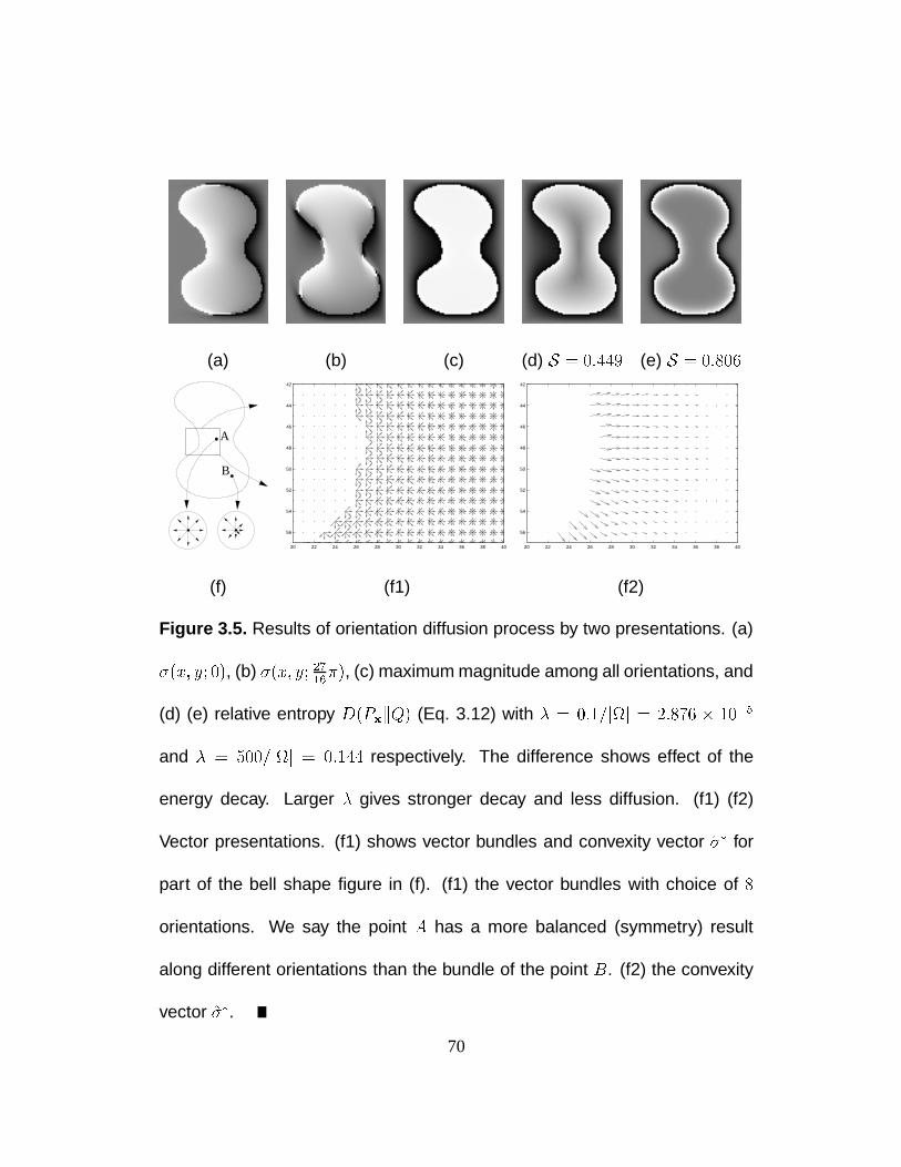
(a) (b) (c) (d) S = 0:449 (e) S = 0:806
B
A
20 22 24 26 28 30 32 34 36 38 40
42
44
46
48
50
52
54
56
20 22 24 26 28 30 32 34 36 38 40
42
44
46
48
50
52
54
56
(f) (f1) (f2)
Figure 3.5. Results of orientation diffusion process by two presentations. (a)
(x; y; 0), (b) (x; y; 2716), (c) maximum magnitude among all orientations, and
(d) (e) relative entropy D(PxkQ) (Eq. 3.12) with = 0:1=jj = 2:876 105
and = 500=jj = 0:144 respectively. The difference shows effect of the
energy decay. Larger gives stronger decay and less diffusion. (f1) (f2)
Vector presentations. (f1) shows vector bundles and convexity vector for
part of the bell shape figure in (f). (f1) the vector bundles with choice of 8
orientations. We say the point A has a more balanced (symmetry) result
along different orientations than the bundle of the point B. (f2) the convexity
vector .
70
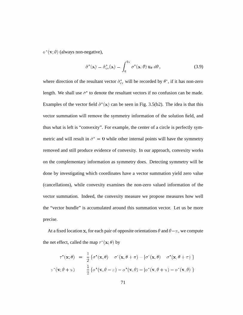
(x; ) (always non-negative),
(x) = cv(x) =
Z 2
0
(x; )u d ; (3.9)
where direction of the resultant vectorcv will be recorded by, if it has non-zero
length. We shall use to denote the resultant vectors if no confusion can be made.
Examples of the vector field(x) can be seen in Fig. 3.5(b2). The idea is that this
vector summation will remove the symmetry information of the solution field, and
thus what is left is “convexity”. For example, the center of a circle is perfectly sym-
metric and will result in = 0 while other internal points will have the symmetry
removed and still produce evidence of convexity. In our approach, convexity works
on the complementary information as symmetry does. Detecting symmetry will be
done by investigating which coordinates have a vector summation yield zero value
(cancellations), while convexity examines the non-zero valued information of the
vector summation. Indeed, the convexity measure we propose measures how well
the “vector bundle” is accumulated around this summation vector. Let us be more
precise.
At a fixed locationx, for each pair of opposite orientations and+, we compute
the net effect, called the map (x; ) by
(x; ) =1
2f(x; ) (x; + ) + j(x; ) (x; + )jg
(x; + ) =1
2f(x; + ) (x; ) + j(x; + ) (x; )jg
71
(a) (b)
Figure 3.6. A simple experiment used for F/G separation and its relative en-
tropy D(PxkQ). While right side is convex and left side is concave, we have
S=S = 0:605=0:671 respectively. Both regions are equally sized.
= (x; ) (x; ) + (x; + ) ; (3.10)
where a cyclic boundary condition = + 2 is used. Note that equation (3.9) can
be rewritten as
(x) =
Z 2
0
(x; )u d :
The second step is to transform(x; ) to P (x; ) or simply Px(), by a linear
transformation, similar to what we did for the decay model in Eq. 2.12. It is
P (x; ) =1
2(1 + (x; )) :
Unlike any previous work, we propose a Kullback-Leibler distance (or relative
entropy) to measure convexity. The mapPx() is compared to a Gaussian map inS1
(not normalized)
Q() =1
1 + Nexp(
( )2
22); (3.11)
72
where the center ofQ is located in the direction, the direction of vector (here
stands for standard deviation, not the diffusion field. It is set to2:0 throughout all the
experiments). A small positive constantN is given to avoid the case ofQ() = 1.
The Kullback-Leibler distance, computed at every pointx, betweenQ() andPx()
is given by
D(PxkQ) =
Z 2
0
Px() logPx()
Q()+ (1 Px()) log
1 Px()
1Q()d : (3.12)
Intuitively, it measures the inefficiency of assuming that the distribution isQ()when
the real distribution isPx(). That is, we assume the map inS1 has a sharp peak at
. D(PxkQ) is always equal to or greater than0, and it can be greater than1. A
smaller measure means a better fit.
This measure is given for each pointx. To obtain a global measure of a shape, we
simply average this measure over the points on the figure, i.e., the final measure of a
shape is
S(Px) =1
jj
Z
D(PxkQ) dx ;
A shape with a smaller measure is considered more convex than others. A simple
example can be seen in Fig. 3.6 as a F/G experiment. We continue to useS to denote
the measure for background area.
73

3.2 Convexity Measurement by 2nd Order Process
The process can be considered as a 2nd order Markov chain with memory of location
and orientation. Various studies suggest that the 2nd order Markov chain with the
help of Kullback-Leibler measure provides better convexity measurement than the
one derived from the decay process. We use numerous experiments to show the
difference between them. The result strongly depends on the appropriate choice of
. But in this section, we will only sketch various experiments that we are interested
and their results. The results derived by using different’s and their relations will be
discussed in Sec. 3.3. Other results are separated in different sections in rest of this
chapter. The comparison of two perfectly convex shapes are discussed in Sec. 3.4.
In Sec. 3.5, we discuss convexity of the shape with minor perturbations in the fine
scales. The implementation details are given in Sec. 3.6.
The first series is organized as F/G experiments. It includes the images with the
concave cusp feature in Fig. 3.3, inspired by Stevens et al. [82] and the convexity-
symmetry images adapted from Kanizsa [39]. Besides the F/G experiments, in the
second series of experiments, we compare convexity of different shapes. It is a
figure-to-figure rather than figure-to-ground comparison. The reason that we com-
pare “figure” to “figure” by this model instead of the decay model is because many
unnecessary attributes in the decay model such as size or symmetry preference have
74
been removed here. Therefore, it is appropriate to mention “convexity measure” of
shapes as it solely owns the name now. The comparison can thus be applied to a
wider range. In most experiments, results from the decay model are provided for
comparison.
3.2.1 Figure/Ground Separation
We examine our measure using four prototypes, a simple arc in Fig. 3.6, the colon-
nade in Fig. 3.7, concave-cusp figures in Fig. 3.8 and the Kanizsa figures in Fig. 3.9.
Shapes with higher convexity win on all trials.
Arc For a F/G experiment of arc shape in Fig. 3.6, the measure is given byS=S =
0:605=0:671, favoring the white region.
Colonnade In the second series shown in Fig. 3.7, we test our measure in colonnade-
figure images. The result is consistent through images with different ratios of bk/wt
area. Also, we do observe the size effect from (a) to (c): the difference between
figures and background becomes less as black/white regions get smaller/larger re-
spectively.
Concave Cusp For concave-cusp images in Fig. 3.8(a) & (b), we apply both of the
decay diffusion and the orientation diffusion process as methods for F/G separation.
75
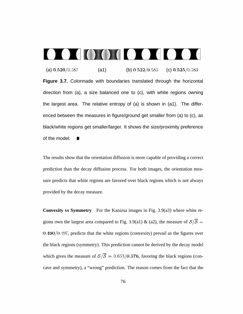
(a) 0:520=0:587 (a1) (b) 0:522=0:585 (c) 0:525=0:583
Figure 3.7. Colonnade with boundaries translated through the horizontal
direction from (a), a size balanced one to (c), with white regions owning
the largest area. The relative entropy of (a) is shown in (a1). The differ-
enced between the measures in figure/ground get smaller from (a) to (c), as
black/white regions get smaller/larger. It shows the size/proximity preference
of the model.
The results show that the orientation diffusion is more capable of providing a correct
prediction than the decay diffusion process. For both images, the orientation mea-
sure predicts that white regions are favored over black regions which is not always
provided by the decay measure.
Convexity vs Symmetry For the Kanizsa images in Fig. 3.9(a3) where white re-
gions own the largest area compared to Fig. 3.9(a1) & (a2), the measure ofS=S =
0:490=0:497, predicts that the white regions (convexity) prevail as the figures over
the black regions (symmetry). This prediction cannot be derived by the decay model
which gives the measure ofS=S = 0:653=0:576, favoring the black regions (con-
cave and symmetry), a “wrong” prediction. The reason comes from the fact that the
76
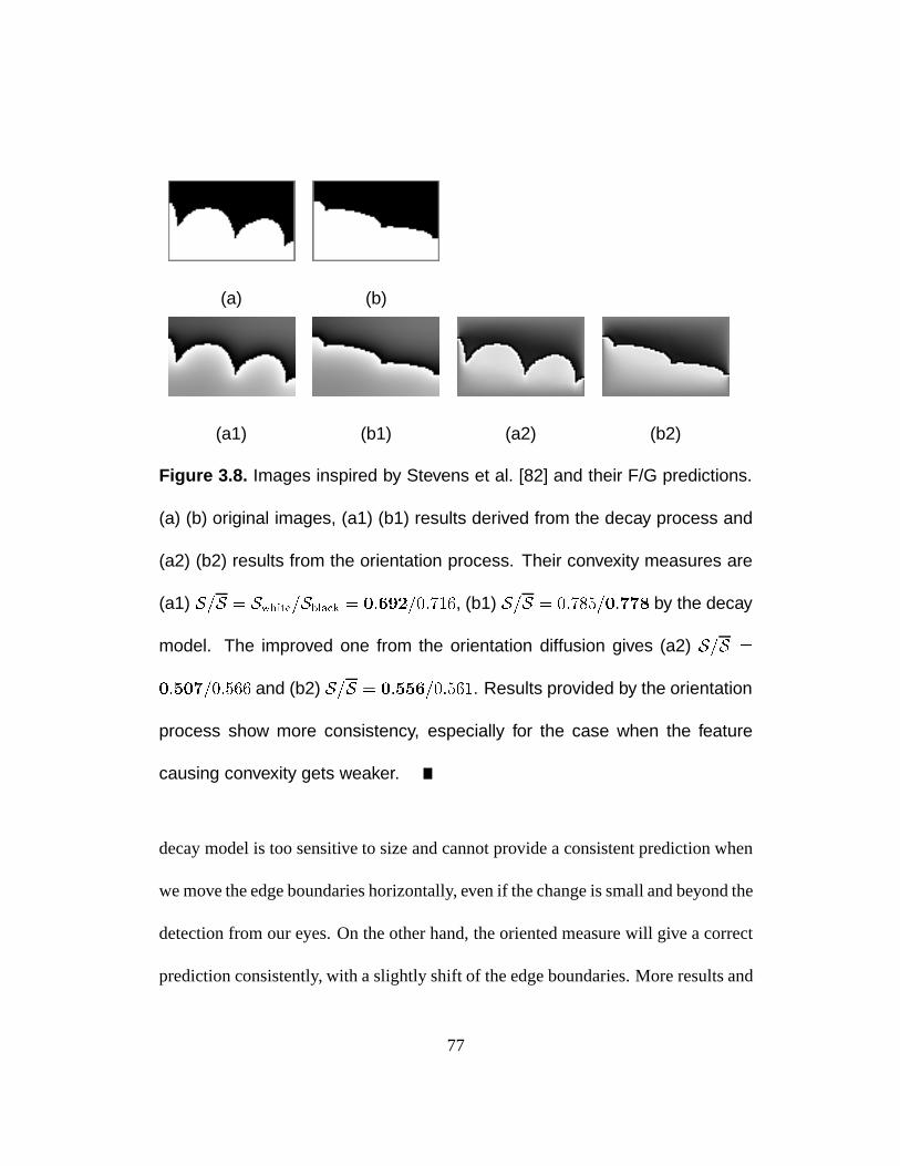
(a) (b)
(a1) (b1) (a2) (b2)
Figure 3.8. Images inspired by Stevens et al. [82] and their F/G predictions.
(a) (b) original images, (a1) (b1) results derived from the decay process and
(a2) (b2) results from the orientation process. Their convexity measures are
(a1) S=S = Swhite=Sblack = 0:692=0:716, (b1) S=S = 0:785=0:778 by the decay
model. The improved one from the orientation diffusion gives (a2) S=S =
0:507=0:566 and (b2) S=S = 0:556=0:561. Results provided by the orientation
process show more consistency, especially for the case when the feature
causing convexity gets weaker.
decay model is too sensitive to size and cannot provide a consistent prediction when
we move the edge boundaries horizontally, even if the change is small and beyond the
detection from our eyes. On the other hand, the oriented measure will give a correct
prediction consistently, with a slightly shift of the edge boundaries. More results and
77
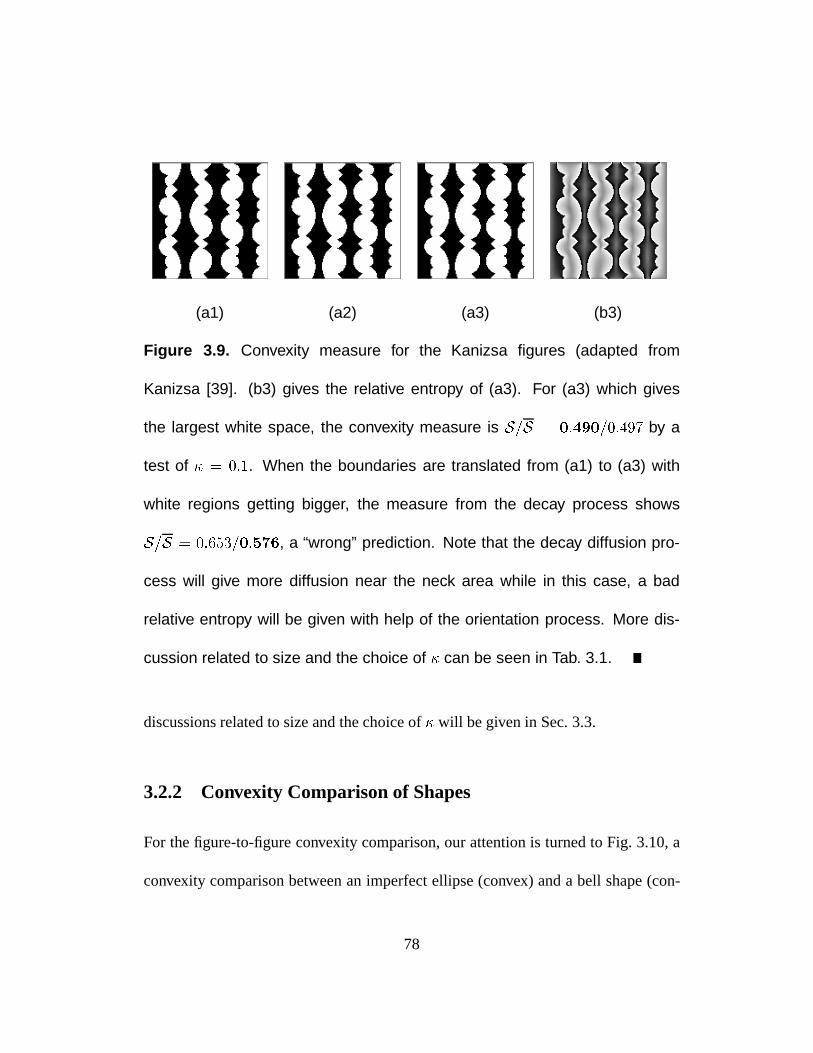
(a1) (a2) (a3) (b3)
Figure 3.9. Convexity measure for the Kanizsa figures (adapted from
Kanizsa [39]. (b3) gives the relative entropy of (a3). For (a3) which gives
the largest white space, the convexity measure is S=S = 0:490=0:497 by a
test of = 0:1. When the boundaries are translated from (a1) to (a3) with
white regions getting bigger, the measure from the decay process shows
S=S = 0:653=0:576, a “wrong” prediction. Note that the decay diffusion pro-
cess will give more diffusion near the neck area while in this case, a bad
relative entropy will be given with help of the orientation process. More dis-
cussion related to size and the choice of can be seen in Tab. 3.1.
discussions related to size and the choice of will be given in Sec. 3.3.
3.2.2 Convexity Comparison of Shapes
For the figure-to-figure convexity comparison, our attention is turned to Fig. 3.10, a
convexity comparison between an imperfect ellipse (convex) and a bell shape (con-
78
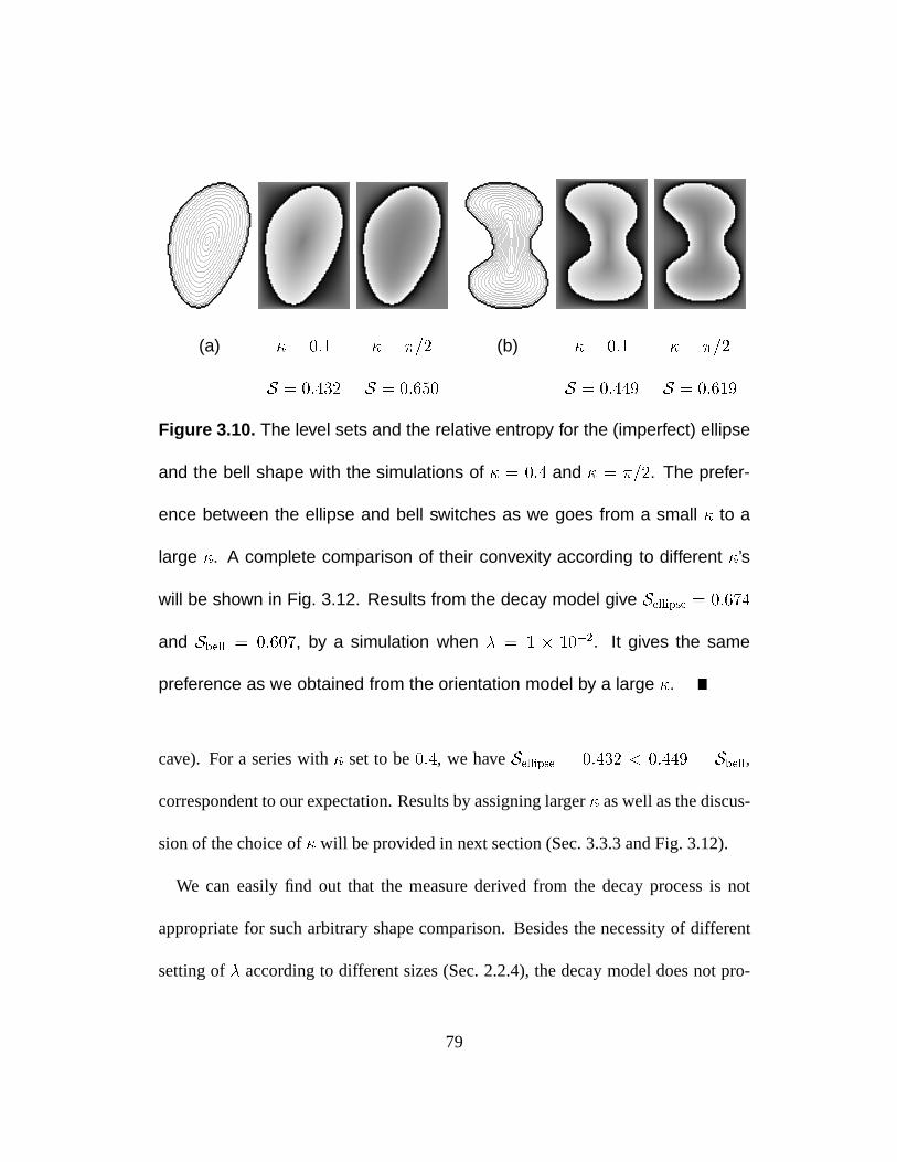
(a) = 0:1 = =2 (b) = 0:1 = =2
S = 0:432 S = 0:650 S = 0:449 S = 0:619
Figure 3.10. The level sets and the relative entropy for the (imperfect) ellipse
and the bell shape with the simulations of = 0:4 and = =2. The prefer-
ence between the ellipse and bell switches as we goes from a small to a
large . A complete comparison of their convexity according to different ’s
will be shown in Fig. 3.12. Results from the decay model give Sellipse = 0:674
and Sbell = 0:607, by a simulation when = 1 102. It gives the same
preference as we obtained from the orientation model by a large .
cave). For a series with set to be0:4, we haveSellipse = 0:432 < 0:449 = Sbell,
correspondent to our expectation. Results by assigning larger as well as the discus-
sion of the choice of will be provided in next section (Sec. 3.3.3 and Fig. 3.12).
We can easily find out that the measure derived from the decay process is not
appropriate for such arbitrary shape comparison. Besides the necessity of different
setting of according to different sizes (Sec. 2.2.4), the decay model does not pro-
79
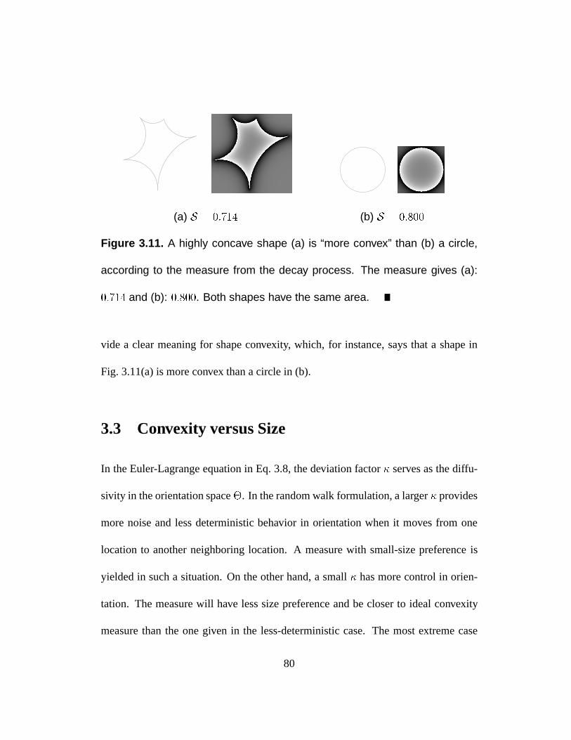
(a) S = 0:714 (b) S = 0:800
Figure 3.11. A highly concave shape (a) is “more convex” than (b) a circle,
according to the measure from the decay process. The measure gives (a):
0:714 and (b): 0:800. Both shapes have the same area.
vide a clear meaning for shape convexity, which, for instance, says that a shape in
Fig. 3.11(a) is more convex than a circle in (b).
3.3 Convexity versus Size
In the Euler-Lagrange equation in Eq. 3.8, the deviation factor serves as the diffu-
sivity in the orientation space. In the random walk formulation, a larger provides
more noise and less deterministic behavior in orientation when it moves from one
location to another neighboring location. A measure with small-size preference is
yielded in such a situation. On the other hand, a small has more control in orien-
tation. The measure will have less size preference and be closer to ideal convexity
measure than the one given in the less-deterministic case. The most extreme case
80
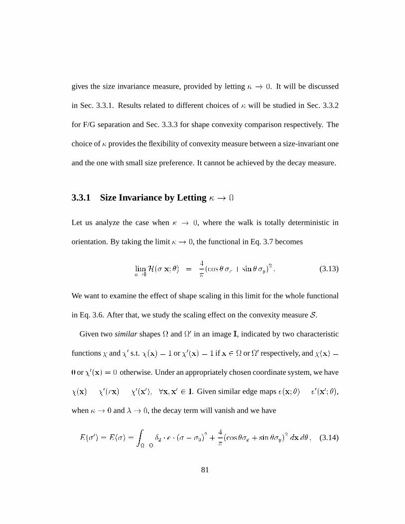
gives the size invariance measure, provided by letting ! 0. It will be discussed
in Sec. 3.3.1. Results related to different choices of will be studied in Sec. 3.3.2
for F/G separation and Sec. 3.3.3 for shape convexity comparison respectively. The
choice of provides the flexibility of convexity measure between a size-invariant one
and the one with small size preference. It cannot be achieved by the decay measure.
3.3.1 Size Invariance by Letting! 0
Let us analyze the case when ! 0, where the walk is totally deterministic in
orientation. By taking the limit! 0, the functional in Eq. 3.7 becomes
lim!0
H(jx; ) =4
(cos x + sin y)
2 : (3.13)
We want to examine the effect of shape scaling in this limit for the whole functional
in Eq. 3.6. After that, we study the scaling effect on the convexity measureS.
Given twosimilar shapes and0 in an imageI, indicated by two characteristic
functions and0 s.t.(x) = 1 or0(x) = 1 if x 2 or0 respectively, and(x) =
0 or0(x) = 0 otherwise. Under an appropriately chosen coordinate system, we have
(x) = 0(rx) = 0(x0); 8x;x0 2 I. Given similar edge mapse(x; ) = e0(x0; ),
when! 0 and! 0, the decay term will vanish and we have
E(0) = E() =
Z
Æ2 e ( 0)2 +
4
(cos x + sin y)
2 dx d ; (3.14)
81
if we assign0(x0; ) = (x; ). So the minimizer for either functional can be ob-
tained easily when the other one has been computed. Two minimizers are related by
(x; ) = 0(x0; ). Different orientations are worked independently here.
Let us discuss the scaling effect on the convexity measure. For two similar maps
, 0, we can obtain the similarity betweenPx andPx0 orD(PxkQ) andD(Px0kQ).
Therefore, for the convexity measure, we have
S(Px0) =1
j0j
Z0D(Px0kQ) dx
0
=1
r2jj r2Z
D(PxkQ) dx = S(Px) : (3.15)
It is an ideal case where we can achieve a measure with no sensitivity to the size.
Examples in the discrete case can be found in Fig. 3.12 and Sec. 3.3.3. When is
not zero, we need to set a smaller0 = =r2 to achieve the similarity(x; ) =
0(x0; ).
3.3.2 Figure/Ground Separation in Convexity-Symmetry Image
We will use the Kanizsa figures in Fig. 3.9 to illustrate our points. As we have
discussed, the decay model cannot provide a consistent prediction when the area
ratio of different regions is changed, even though the change is small and beyond the
detection from our eyes. The orientation model will give a consistent prediction, with
a small shift of edge boundaries. The trick lies in the free parameter which on one
82
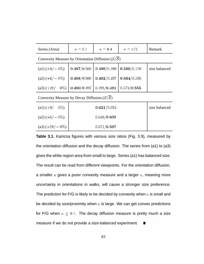
Series (Area) = 0:1 = 0:4 = =2 Remark
Convexity Measure by Orientation Diffusion (S=S)
(a1) (+0= 0%) 0:487=0:502 0:490=0:499 0:560=0:570 size balanced
(a2) (+6= 0%) 0:488=0:500 0:492=0:497 0:564=0:565
(a3) (+28= 0%) 0:490=0:497 0:495=0:491 0:573=0:555
Convexity Measure by Decay Diffusion (S=S)
(a1) (+0= 0%) 0:621=0:653 size balanced
(a2) (+6= 0%) 0:638=0:635
(a3) (+28= 0%) 0:671=0:597
Table 3.1. Kanizsa figures with various size ratios (Fig. 3.9), measured by
the orientation diffusion and the decay diffusion. The series from (a1) to (a3)
gives the white region area from small to large. Series (a1) has balanced size.
The result can be read from different viewpoints. For the orientation diffusion,
a smaller gives a purer convexity measure and a larger , meaning more
uncertainty in orientations in walks, will cause a stronger size preference.
The prediction for F/G is likely to be decided by convexity when is small and
be decided by size/proximity when is large. We can get convex predictions
for F/G when 0:1. The decay diffusion measure is pretty much a size
measure if we do not provide a size-balanced experiment.
83
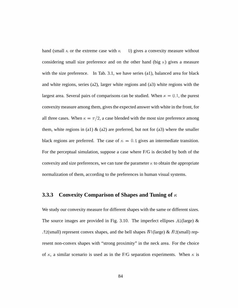
hand (small or the extreme case with = 0) gives a convexity measure without
considering small size preference and on the other hand (big) gives a measure
with the size preference. In Tab. 3.1, we have series (a1), balanced area for black
and white regions, series (a2), larger white regions and (a3) white regions with the
largest area. Several pairs of comparisons can be studied. When = 0:1, the purest
convexity measure among them, gives the expected answer with white in the front, for
all three cases. When = =2, a case blended with the most size preference among
them, white regions in (a1) & (a2) are preferred, but not for (a3) where the smaller
black regions are preferred. The case of = 0:4 gives an intermediate transition.
For the perceptual simulation, suppose a case where F/G is decided by both of the
convexity and size preferences, we can tune the parameter to obtain the appropriate
normalization of them, according to the preferences in human visual systems.
3.3.3 Convexity Comparison of Shapes and Tuning of
We study our convexity measure for different shapes with the same or different sizes.
The source images are provided in Fig. 3.10. The imperfect ellipsesA1(large) &
A2(small) represent convex shapes, and the bell shapesB1(large) &B2(small) rep-
resent non-convex shapes with “strong proximity” in the neck area. For the choice
of , a similar scenario is used as in the F/G separation experiments. When is
84
0 0.2 0.4 0.6 0.8 1 1.2 1.4 1.6
0.4
0.45
0.5
0.55
0.6
0.65
Deviation Parameter
Rel
ativ
e E
ntro
py
Relative Entropy for Various Shapes
ellipse A1: area=3324small ellipse A2: area=1682bell B1: area=3477small bell B2: area=1652
Figure 3.12. A comparison between shapes with different sizes and convex-
ity. Four curves listed in = =2, from top to bottom are for the (imperfect)
ellipse A1, bell B1, small ellipse A2 and small bell B2, shown in Fig. 3.10. A
measure with small will pick shapes by convexity. A measure with large
will pick shapes by size/proximity; therefore, either small sized shapes or the
bells which own strong proximity near the neck will be favored. When = 0:1,
the case with the least size preference, the measures for all similar shapes
with different sizes will coincide with each other.
85
small, we pick shape by convexity and when is larger, we either pick the smaller
size shapes or pick the bell shape with stronger proximity. The details are shown in
Fig. 3.12.
Convexity comparison of shapes with the same sizeWhen two shapes share the
same size, we can easily pick up the ellipse as the more convex shape by choosing
0:6. A large will favor proximity and therefore pick the bell as the more
favorable shape. We haveSA1 < SB1 andSA2 < SB2 when 0:6.
Convexity comparison of shapes with any sizesTo make the measure capable to
be applied in a wider range, we compare shapes with different sizes, achieved by
using an even smaller 0:4. In this case, no size/proximity issues need to be
considered and the measure becomes a “convexity measure”. We haveSA1;SA2 <
SB1;SB2 if 0:4 is provided. The smallest or = 0:1 provides a measure
with the least sensitivity to the size. As we can see, the values of similar shapes with
different sizes are coincided to each other in this situation.
Large and size/proximity preference When is large, it is the case of diffusion
with low certainty in orientation. We will have the result favoring smaller size shapes,
as we haveSA2;SB2 < SA1;SB1. When similar size shapes are compared, a shape
with stronger proximity will prevail. Therefore, the bellB1 is favored over the ellipse
86
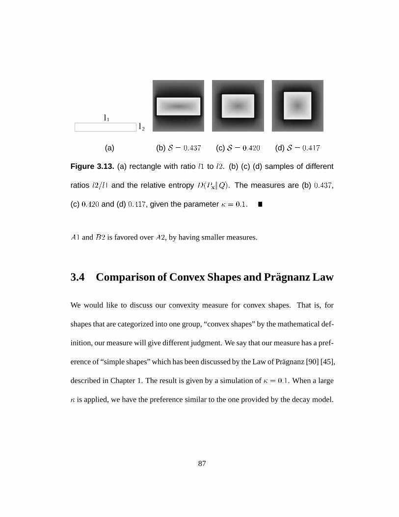
l 2
1l
(a) (b) S = 0:437 (c) S = 0:420 (d) S = 0:417
Figure 3.13. (a) rectangle with ratio l1 to l2. (b) (c) (d) samples of different
ratios l2=l1 and the relative entropy D(PxkQ). The measures are (b) 0:437,
(c) 0:420 and (d) 0:417, given the parameter = 0:1.
A1 andB2 is favored overA2, by having smaller measures.
3.4 Comparison of Convex Shapes and Pragnanz Law
We would like to discuss our convexity measure for convex shapes. That is, for
shapes that are categorized into one group, “convex shapes” by the mathematical def-
inition, our measure will give different judgment. We say that our measure has a pref-
erence of “simple shapes” which has been discussed by the Law of Pr¨agnanz [90] [45],
described in Chapter 1. The result is given by a simulation of = 0:1. When a large
is applied, we have the preference similar to the one provided by the decay model.
87
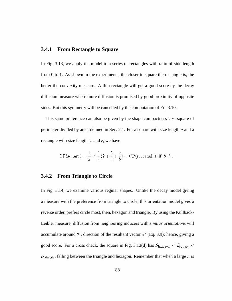
3.4.1 From Rectangle to Square
In Fig. 3.13, we apply the model to a series of rectangles with ratio of side length
from 0 to 1. As shown in the experiments, the closer to square the rectangle is, the
better the convexity measure. A thin rectangle will get a good score by the decay
diffusion measure where more diffusion is promised by good proximity of opposite
sides. But this symmetry will be cancelled by the computation of Eq. 3.10.
This same preference can also be given by the shape compactnessCP, square of
perimeter divided by area, defined in Sec. 2.1. For a square with size lengtha and a
rectangle with size lengthsb andc, we have
CP(square) =4
<
1
(2 +
b
c+c
b) = CP(rectangle) if b 6= c :
3.4.2 From Triangle to Circle
In Fig. 3.14, we examine various regular shapes. Unlike the decay model giving
a measure with the preference from triangle to circle, this orientation model gives a
reverse order, prefers circle most, then, hexagon and triangle. By using the Kullback-
Leibler measure, diffusion from neighboring inducers withsimilar orientationswill
accumulate around, direction of the resultant vector (Eq. 3.9); hence, giving a
good score. For a cross check, the square in Fig. 3.13(d) hasShexagon < Ssquare <
Striangle, falling between the triangle and hexagon. Remember that when a large is
88
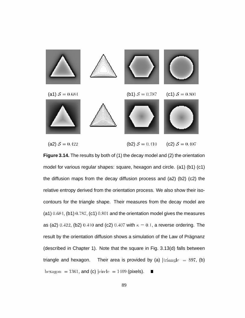
(a1) S = 0:684 (b1) S = 0:787 (c1) S = 0:801
(a2) S = 0:422 (b2) S = 0:410 (c2) S = 0:407
Figure 3.14. The results by both of (1) the decay model and (2) the orientation
model for various regular shapes: square, hexagon and circle. (a1) (b1) (c1)
the diffusion maps from the decay diffusion process and (a2) (b2) (c2) the
relative entropy derived from the orientation process. We also show their iso-
contours for the triangle shape. Their measures from the decay model are
(a1) 0:684, (b1) 0:787, (c1) 0:801 and the orientation model gives the measures
as (a2) 0:422, (b2) 0:410 and (c2) 0:407 with = 0:1, a reverse ordering. The
result by the orientation diffusion shows a simulation of the Law of Pragnanz
(described in Chapter 1). Note that the square in Fig. 3.13(d) falls between
triangle and hexagon. Their area is provided by (a) jtrianglej = 897, (b)
jhexagonj = 1361, and (c) jcirclej = 1469 (pixels).
89
applied, we have the reverse preference, the same as the one provided by the decay
measure.
The shape compactnessCP will also give the same order of preference. As we
have discussed in Sec. 2.1, the shape compactness is not appropriate to be applied
in F/G problems. For balanced-sized regions, shape compactness will give the same
result if the image frame is not considered to be part of the shape boundaries. On the
other hand, larger regions will be selected, opposite to our perception, if we do con-
sider the image frame as part of the shape boundaries. The results created by different
considerations of the image frame will be discussed in Sec. 3.6.1. Another difference
between the shape compactness measure and the orientation diffusion measure is
that they have different considerations for structures in different scales. It will be
discussed in Sec. 3.5.
3.5 Coarse Scale Structures
The decay diffusion process is not appropriate to measure convexity of shapes with
small perturbations in fine scales as in Fig. 3.15 or Fig. 3.16. Due to the exponential
drop in the energy, the measure derived from the decay process catches only the
properties in fine scales. But for the shapes in (a1) and (a2), we are more interested
in the global properties which describe them as circles up to some noise on fine
90
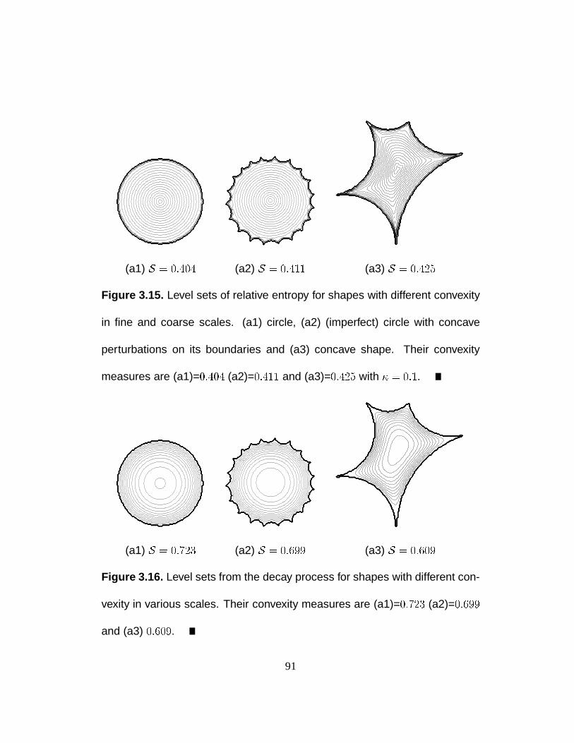
(a1) S = 0:404 (a2) S = 0:411 (a3) S = 0:425
Figure 3.15. Level sets of relative entropy for shapes with different convexity
in fine and coarse scales. (a1) circle, (a2) (imperfect) circle with concave
perturbations on its boundaries and (a3) concave shape. Their convexity
measures are (a1)=0:404 (a2)=0:411 and (a3)=0:425 with = 0:1.
(a1) S = 0:723 (a2) S = 0:699 (a3) S = 0:609
Figure 3.16. Level sets from the decay process for shapes with different con-
vexity in various scales. Their convexity measures are (a1)=0:723 (a2)=0:699
and (a3) 0:609.
91
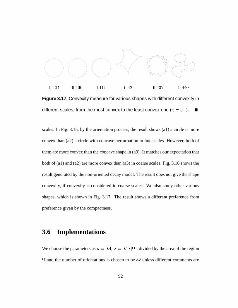
0:404 0:406 0:411 0:425 0:437 0:440
Figure 3.17. Convexity measure for various shapes with different convexity in
different scales, from the most convex to the least convex one ( = 0:1).
scales. In Fig. 3.15, by the orientation process, the result shows (a1) a circle is more
convex than (a2) a circle with concave perturbation in fine scales. However, both of
them are more convex than the concave shape in (a3). It matches our expectation that
both of (a1) and (a2) are more convex than (a3) in coarse scales. Fig. 3.16 shows the
result generated by the non-oriented decay model. The result does not give the shape
convexity, if convexity is considered in coarse scales. We also study other various
shapes, which is shown in Fig. 3.17. The result shows a different preference from
preference given by the compactness.
3.6 Implementations
We choose the parameters as = 0:4, = 0:1=jj, divided by the area of the region
and the number of orientations is chosen to be32 unless different comments are
92
made. The 2-D delta function is chosen in the same manner as we did in the decay
diffusion process and the delta function coefficient is chosen to be = 105 j@j,
a constant normalized by the perimeter of. The normalization of the parameters
and according to area and perimeter of respectively is not essential for the
convexity measurement. As we discussed in Sec. 3.3.1, a small enough and can
bring us to a measurement close to a size-invariance one. The standard deviation
used in the Kullback-Leibler measure is set to be2:0 all the times unless different
comment is given.
3.6.1 Boundary Condition and Shape Surroundedness
We adopt the absorbing barriers as boundary/frame condition throughout our sim-
ulations. We would like to give an example to illustrate how different choices of
boundary condition/shape surroundedness can lead to different judgment of salience.
In the image where size/proximity can dominately decide the F/G phenomenon
(e.g., Fig. 2.7 (c)) we can use the orientation measure to predict the “correct” F/G.
On the other hand, a different boundary/frame consideration can be made where
the image frame is also considered as inducer boundaries. The salience competi-
tion becomes the comparison between the (closed-) thinner rectangle shapes and the
(closed-) thicker rectangle shapes. The study in Sec. 3.4.1 suggests that the black
93

thicker rectangles, closer to squares, will have a better convexity measure, therefore
provide a different answer. The preference of the white regions in our visual system
supports the first choice of boundary condition. It implies thatimage frames should
not be considered as part of the shape boundaries.
We would like to relate our models, either the decay model or the orientation
model, to the issue of shape surroundedness which is known to be one of the fac-
tors affecting the decision of salience. We can easily understand it from our models,
with or without the orientation consideration. It predicts that shapes with full sur-
rounded boundaries will have better/smaller measure than the ones without closed
boundaries.
94
Chapter 4
Internal Shape Representation
4.1 Symmetry Information
To illustrate that internal shape representation is included in our diffusion models, we
compute shape axis. The idea that shape axis can be captured by our diffusion models
is not particularly new or surprising. For example, based on the work of Siddiqi and
Kimia [80] or Kimia et al. [44], we know that the diffusion process over shapes will
“meet” (yield shocks) at the symmetry axis. However, the results from our models,
based on variational approaches are provided in the static state. Therefore, the def-
inition of axis will no longer be decided by pairs of points, but a global property of
the boundaries. The term “shape axis” is used instead of “symmetry axis” or “medial
axis” to distinguish from the axis generally mentioned in the medial axis transform or
95
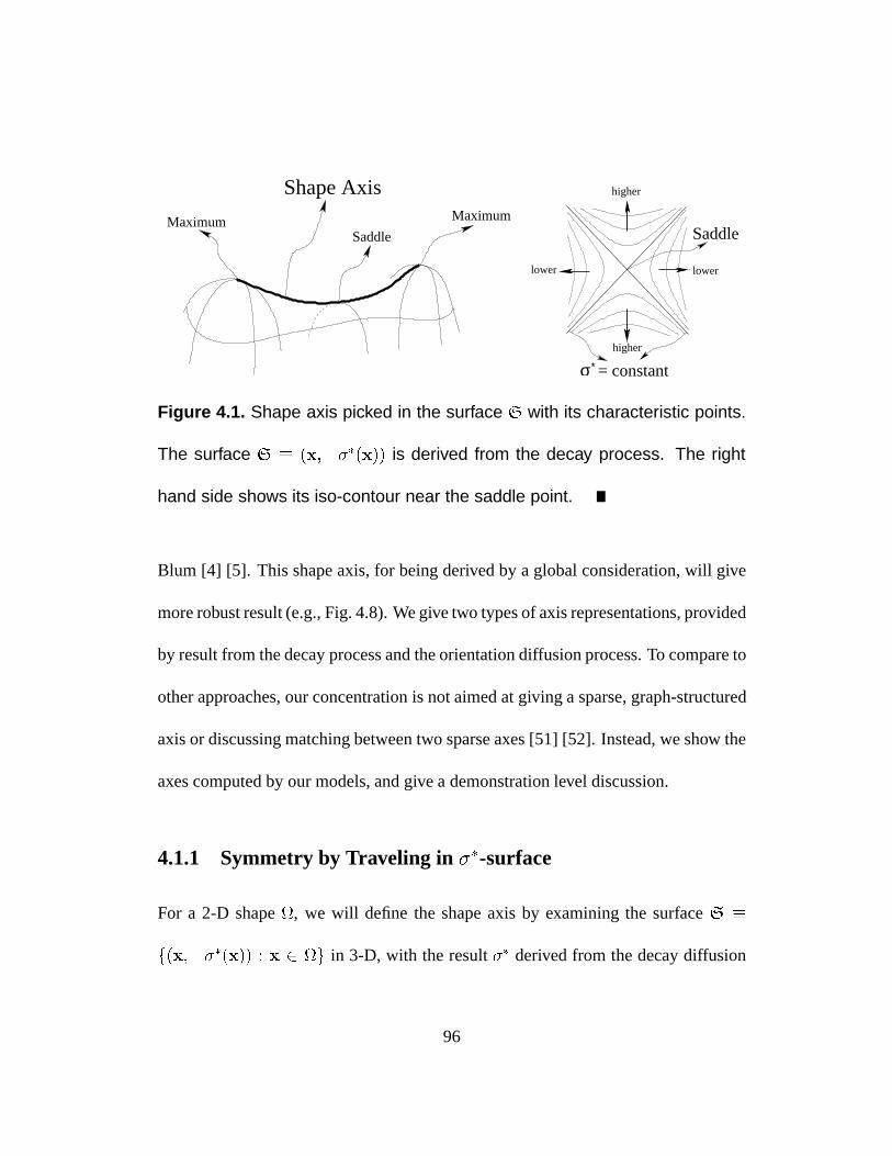
MaximumSaddle
Maximum
Shape Axis
∗σ = constant
lower lower
higher
higher
Saddle
Figure 4.1. Shape axis picked in the surface S with its characteristic points.
The surface S (x;(x)) is derived from the decay process. The right
hand side shows its iso-contour near the saddle point.
Blum [4] [5]. This shape axis, for being derived by a global consideration, will give
more robust result (e.g., Fig. 4.8). We give two types of axis representations, provided
by result from the decay process and the orientation diffusion process. To compare to
other approaches, our concentration is not aimed at giving a sparse, graph-structured
axis or discussing matching between two sparse axes [51] [52]. Instead, we show the
axes computed by our models, and give a demonstration level discussion.
4.1.1 Symmetry by Traveling in-surface
For a 2-D shape, we will define the shape axis by examining the surfaceS
f(x;(x)) : x 2 g in 3-D, with the result derived from the decay diffusion
96
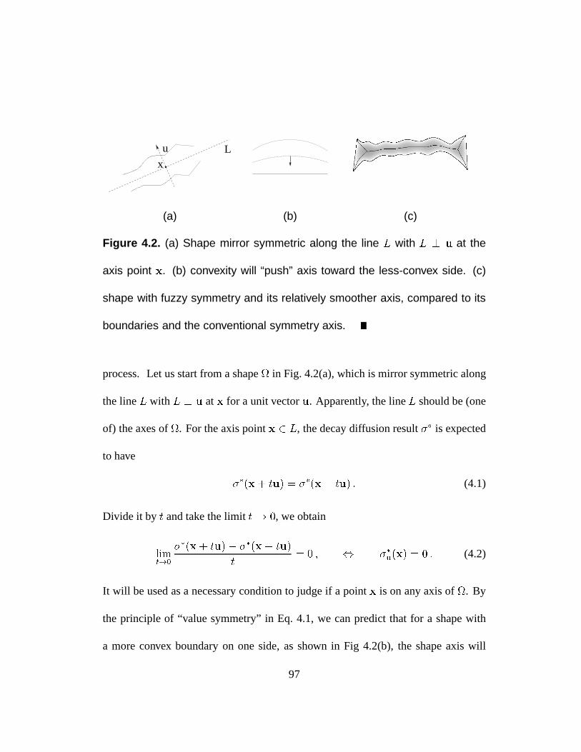
u Lx
(a) (b) (c)
Figure 4.2. (a) Shape mirror symmetric along the line L with L ? u at the
axis point x. (b) convexity will “push” axis toward the less-convex side. (c)
shape with fuzzy symmetry and its relatively smoother axis, compared to its
boundaries and the conventional symmetry axis.
process. Let us start from a shape in Fig. 4.2(a), which is mirror symmetric along
the lineL with L ? u atx for a unit vectoru. Apparently, the lineL should be (one
of) the axes of. For the axis pointx 2 L, the decay diffusion result is expected
to have
(x+ tu) = (x tu) : (4.1)
Divide it by t and take the limitt! 0, we obtain
limt!0
(x+ tu) (x tu)
t= 0 ; ,
u(x) = 0 : (4.2)
It will be used as a necessary condition to judge if a pointx is on any axis of. By
the principle of “value symmetry” in Eq. 4.1, we can predict that for a shape with
a more convex boundary on one side, as shown in Fig 4.2(b), the shape axis will
97
appear near the less-convex side, if the axis does exist. It is because points in the
convex side will get stronger support from the boundary inducers (Sec. 2.2). This
fact makes the shape axis different from the conventional symmetry axis. We define
the shape axis setA to be the projection (to the planez = 0) of the curve setC where
each length-parametrized curveC(s) 2 C satisfies:
1. The curveC(s) is a curve going from one characteristic point to another char-
acteristic point onS. The set of characteristic points includes saddle points,
local maxima and junctions .
2. At each pointx 2 C(s), in direction of the curve normaln, we haven(x) = 0,
satisfying the necessary condition Eq. 4.2.
To meet the first condition, e.g., for the surface of a half sphere, we have only the
projected circle center as the “axis”. Because there is only one characteristic point
on the surface, the maxima in the middle. Before giving the algorithm to compute
the axis, let us discuss those characteristic points. The maximum is caught by
r = (x; y) = 0 ;
with a positive Hessian matrixH s.t.
tTHt = tT
2664 xx xy
yx yy
3775 t 0 ; 8t 6= 0
We mean the place onS where its projection onz = 0 forms a junction of.
98
with the row matrixtT denoting transpose oft = (u; v), the small change aroundx.
Similarly, we can find the minimum if we havetTHt 0, 8t 6= 0. When either of
them happens for differentt’s, we find the saddle point or we can use the equivalent
criteria
det(H) = xxyy xy
2 < 0 ;
evaluated at the pointx. In our algorithm,the junction information will be given as
an input.
We collect all axis points by traveling through the curves from a characteristic point
to another characteristic point. We choose the “uphill” direction. By the maximum
principle, the field will decay from the shape boundaries to interior part of the
shape (meaning(x;(x)) will be rising from the boundaries). Therefore, the only
possible trials fitting the condition (1) are trials from a saddle point or a junction to a
maximum point or another saddle point. The algorithm to find the axes is therefore
given by an initial step and a recursive step:
i Find the maximum points and saddle points on the surfaceS.
ii Start from each saddle point and junction, we choose the most steepest uphill
direction to visit, until any maximum is reached.
2-D projection of these trails, including all the maxima and saddle points are called
the maximum shape axes or shape axes, opposite to those axes going downhill from
99
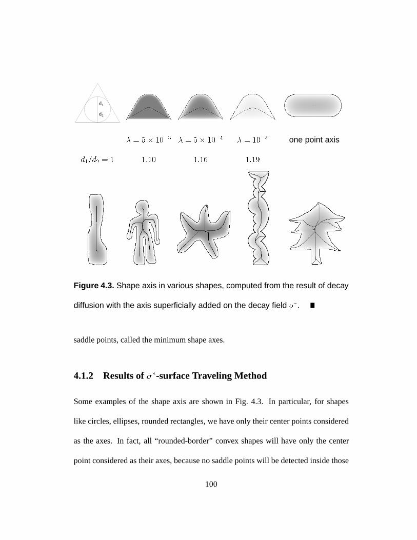
2
d1
d
= 5 103 = 5 104 = 105 one point axis
d1=d2 = 1 1:10 1:16 1:19
Figure 4.3. Shape axis in various shapes, computed from the result of decay
diffusion with the axis superficially added on the decay field .
saddle points, called the minimum shape axes.
4.1.2 Results of-surface Traveling Method
Some examples of the shape axis are shown in Fig. 4.3. In particular, for shapes
like circles, ellipses, rounded rectangles, we have only their center points considered
as the axes. In fact, all “rounded-border” convex shapes will have only the center
point considered as their axes, because no saddle points will be detected inside those
100
shapes.
To compare the shape axis and the traditional medial axis, we can refer the shape
axes found in Fig. 4.3. In the first row, three shapes are designed by regular triangles
with upper angles substituted by their inscribing circles. Their axes found here are
lower than their medial axes which should stay in the middle of the shapes. We say
that the shape axis is “smoother” than the medial axis defined by Blum [4], especially
when the decay coefficient is small. In Fig. 4.2(c), we have smoother axes than its
boundaries and medial axes.
4.1.3 Symmetry by Local Computation Method
We would like to define another set of shape axes by alocal computation method,
based on the result of orientation diffusion process. We would like to emphasize the
differences of this method from previous approaches.
i The axis information given by this method will not be binary represented.
Namely, instead of giving information to tell if a point is on an axis or not, we
compute a map to describe “how likely” a point is on an axis or how “strong”
the axis is.
ii We use a local computation technique to catch the shape axis. The axis will be
locally decided by the result from orientation process. Once the computation
101
of the process is finished, the step to collect shape axes is relatively easier and
more robust than the approach used in other axis generators.
iii The junction feature considered as special axis points, will be collected by a
similar computation.
In our approach, the axis is shown by a continuous map. The continuous information
give us more clue to distinguish between main axis and minor axis. The minor axis
will be declared by a weak representation, e.g., the weak axis created by an obtuse
angle (first order shock) or a pair of weakly mirror-symmetric boundaries (higher or-
der shock) (Fig. 4.4 - 4.8). It provides a natural way of axis pruning if there is a need.
For the second topic, the robustness of our approach comes from two levels. The
local computation is robust, compared to, e.g., the traveling method used in the pre-
vious section. Because missing the detection of an axis point can prevent any further
exploration and miss an axis branch. Secondly, the robustness of our computation
comes from the fact that the shape axis computed by us are based on a global prop-
erty of the shape. We examine the effect of protrusion created on shape boundaries
in Fig. 4.8. The result show that we are able to deal with shape boundaries with small
protrusion (ignore), boundaries with large protrusion (surrender proportionally) with
a transition between them. The third topic as well as the junction detection will be
discussed in next section (Sec. 4.2).
102
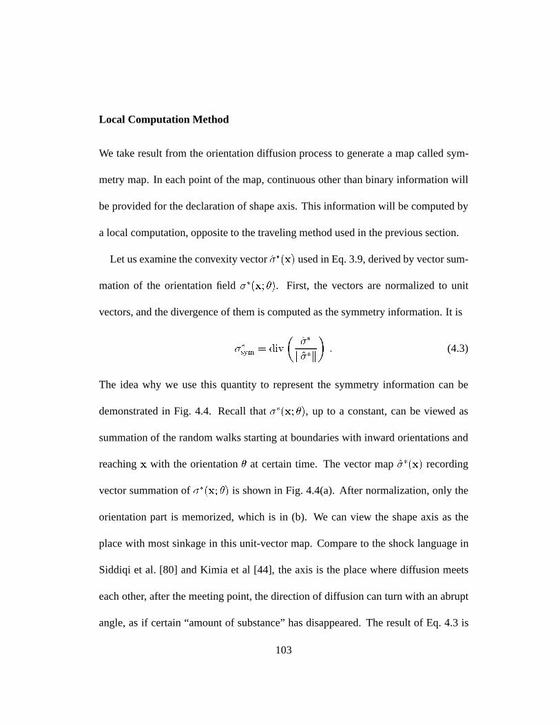
Local Computation Method
We take result from the orientation diffusion process to generate a map called sym-
metry map. In each point of the map, continuous other than binary information will
be provided for the declaration of shape axis. This information will be computed by
a local computation, opposite to the traveling method used in the previous section.
Let us examine the convexity vector(x) used in Eq. 3.9, derived by vector sum-
mation of the orientation field(x; ). First, the vectors are normalized to unit
vectors, and the divergence of them is computed as the symmetry information. It is
sym = div
kk
: (4.3)
The idea why we use this quantity to represent the symmetry information can be
demonstrated in Fig. 4.4. Recall that(x; ), up to a constant, can be viewed as
summation of the random walks starting at boundaries with inward orientations and
reachingx with the orientation at certain time. The vector map(x) recording
vector summation of(x; ) is shown in Fig. 4.4(a). After normalization, only the
orientation part is memorized, which is in (b). We can view the shape axis as the
place with most sinkage in this unit-vector map. Compare to the shock language in
Siddiqi et al. [80] and Kimia et al [44], the axis is the place where diffusion meets
each other, after the meeting point, the direction of diffusion can turn with an abrupt
angle, as if certain “amount of substance” has disappeared. The result of Eq. 4.3 is
103
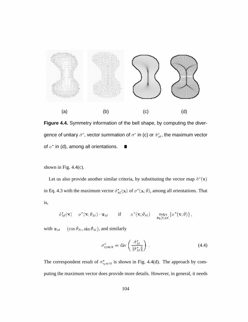
(a) (b) (c) (d)
Figure 4.4. Symmetry information of the bell shape, by computing the diver-
gence of unitary , vector summation of in (c) or M , the maximum vector
of in (d), among all orientations.
shown in Fig. 4.4(c).
Let us also provide another similar criteria, by substituting the vector map(x)
in Eq. 4.3 with the maximum vectorM(x) of (x; ), among all orientations. That
is,
M(x) = (x; M) uM if (x; M) = max2[0;2)
f(x; )g ;
with uM = (cos M ; sin M ), and similarly
symM = div
MkMk
: (4.4)
The correspondent result ofsymM is shown in Fig. 4.4(d). The approach by com-
puting the maximum vector does provide more details. However, in general, it needs
104
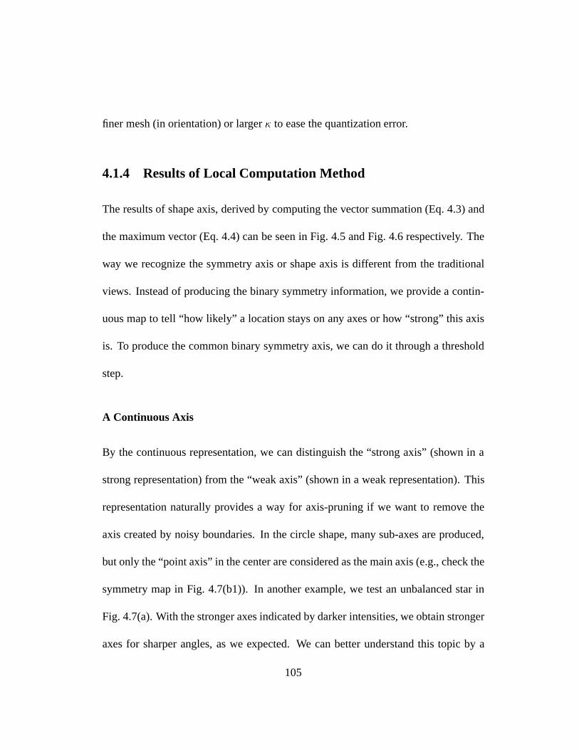
finer mesh (in orientation) or larger to ease the quantization error.
4.1.4 Results of Local Computation Method
The results of shape axis, derived by computing the vector summation (Eq. 4.3) and
the maximum vector (Eq. 4.4) can be seen in Fig. 4.5 and Fig. 4.6 respectively. The
way we recognize the symmetry axis or shape axis is different from the traditional
views. Instead of producing the binary symmetry information, we provide a contin-
uous map to tell “how likely” a location stays on any axes or how “strong” this axis
is. To produce the common binary symmetry axis, we can do it through a threshold
step.
A Continuous Axis
By the continuous representation, we can distinguish the “strong axis” (shown in a
strong representation) from the “weak axis” (shown in a weak representation). This
representation naturally provides a way for axis-pruning if we want to remove the
axis created by noisy boundaries. In the circle shape, many sub-axes are produced,
but only the “point axis” in the center are considered as the main axis (e.g., check the
symmetry map in Fig. 4.7(b1)). In another example, we test an unbalanced star in
Fig. 4.7(a). With the stronger axes indicated by darker intensities, we obtain stronger
axes for sharper angles, as we expected. We can better understand this topic by a
105
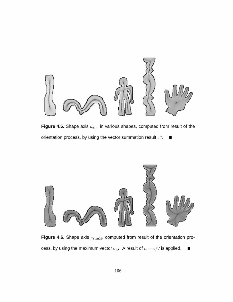
Figure 4.5. Shape axis sym in various shapes, computed from result of the
orientation process, by using the vector summation result .
Figure 4.6. Shape axis symM, computed from result of the orientation pro-
cess, by using the maximum vector M . A result of = =2 is applied.
106
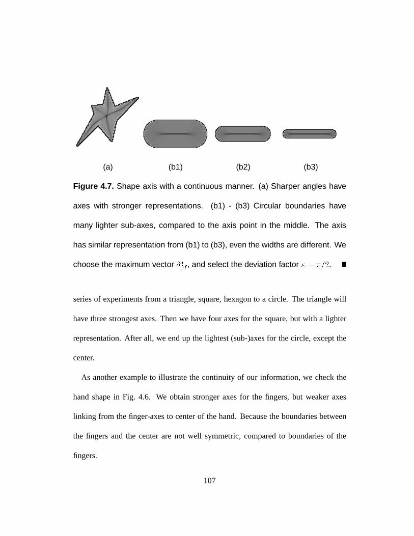
(a) (b1) (b2) (b3)
Figure 4.7. Shape axis with a continuous manner. (a) Sharper angles have
axes with stronger representations. (b1) - (b3) Circular boundaries have
many lighter sub-axes, compared to the axis point in the middle. The axis
has similar representation from (b1) to (b3), even the widths are different. We
choose the maximum vector M , and select the deviation factor = =2.
series of experiments from a triangle, square, hexagon to a circle. The triangle will
have three strongest axes. Then we have four axes for the square, but with a lighter
representation. After all, we end up the lightest (sub-)axes for the circle, except the
center.
As another example to illustrate the continuity of our information, we check the
hand shape in Fig. 4.6. We obtain stronger axes for the fingers, but weaker axes
linking from the finger-axes to center of the hand. Because the boundaries between
the fingers and the center are not well symmetric, compared to boundaries of the
fingers.
107
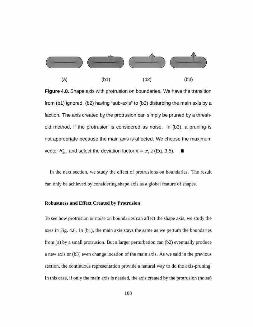
(a) (b1) (b2) (b3)
Figure 4.8. Shape axis with protrusion on boundaries. We have the transition
from (b1) ignored, (b2) having “sub-axis” to (b3) disturbing the main axis by a
faction. The axis created by the protrusion can simply be pruned by a thresh-
old method, if the protrusion is considered as noise. In (b3), a pruning is
not appropriate because the main axis is affected. We choose the maximum
vector M , and select the deviation factor = =2 (Eq. 3.5).
In the next section, we study the effect of protrusions on boundaries. The result
can only be achieved by considering shape axis as a global feature of shapes.
Robustness and Effect Created by Protrusion
To see how protrusion or noise on boundaries can affect the shape axis, we study the
axes in Fig. 4.8. In (b1), the main axis stays the same as we perturb the boundaries
from (a) by a small protrusion. But a larger perturbation can (b2) eventually produce
a new axis or (b3) even change location of the main axis. As we said in the previous
section, the continuous representation provide a natural way to do the axis-pruning.
In this case, if only the main axis is needed, the axis created by the protrusion (noise)
108
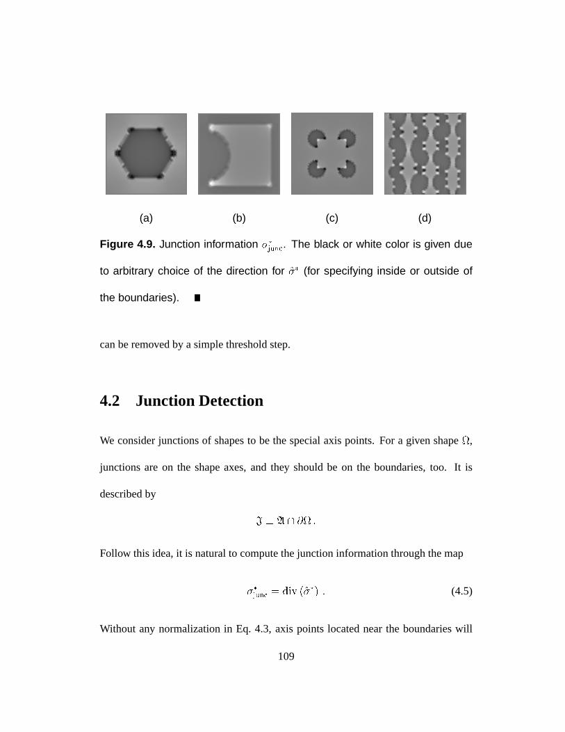
(a) (b) (c) (d)
Figure 4.9. Junction information junc. The black or white color is given due
to arbitrary choice of the direction for (for specifying inside or outside of
the boundaries).
can be removed by a simple threshold step.
4.2 Junction Detection
We consider junctions of shapes to be the special axis points. For a given shape,
junctions are on the shape axes, and they should be on the boundaries, too. It is
described by
J A \ @ :
Follow this idea, it is natural to compute the junction information through the map
junc = div () : (4.5)
Without any normalization in Eq. 4.3, axis points located near the boundaries will
109
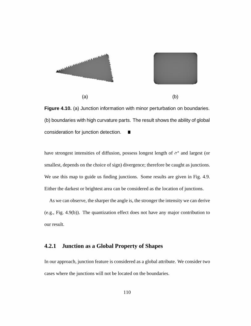
(a) (b)
Figure 4.10. (a) Junction information with minor perturbation on boundaries.
(b) boundaries with high curvature parts. The result shows the ability of global
consideration for junction detection.
have strongest intensities of diffusion, possess longest length of and largest (or
smallest, depends on the choice of sign) divergence; therefore be caught as junctions.
We use this map to guide us finding junctions. Some results are given in Fig. 4.9.
Either the darkest or brightest area can be considered as the location of junctions.
As we can observe, the sharper the angle is, the stronger the intensity we can derive
(e.g., Fig. 4.9(b)). The quantization effect does not have any major contribution to
our result.
4.2.1 Junction as a Global Property of Shapes
In our approach, junction feature is considered as a global attribute. We consider two
cases where the junctions will not be located on the boundaries.
110

When the boundaries have minor perturbations, we can still collect correct infor-
mation even if only the junction feature in the coarsest scale is needed. In Fig. 4.10(a),
our approach provides correct detection for a triangle with noisy boundaries. The
perturbations, if there is any, can create only “minor” junctions.
In our approach, we do not consider junction feature as a binary information. In-
stead, we provide the transition from curves with low curvature to high curvature,
and eventually become discontinuous. In Fig. 4.10(b), a rounded square is tested,
and an easied junction information is obtained.
111

112
Chapter 5
Visual Organization
5.1 Introduction
Discovering perceptual organizations is understood as the transition from low-level
vision to high-level vision. Without the help from object naming, pixels are formed
as surfaces abstractly or symbolically during this process. The illusory figures, such
as the Kanizsa square shows an example where the intensity edges are not the only
information matters for such intergration, but also geometry of the edges. Fig. 5.1
(a1) gives another example of illusory figures. The open edges around the empty
space show cues for occlusions, implying the surface completion with a triangle in
the middle. To describe this choice of completion, first of all, the triangle border
gives a good (linear) continuation. Secondly, unlike the figure given in (a2), the
113
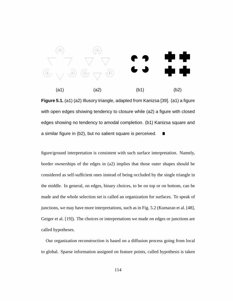
(a1) (a2) (b1) (b2)
Figure 5.1. (a1) (a2) Illusory triangle, adapted from Kanizsa [39]. (a1) a figure
with open edges showing tendency to closure while (a2) a figure with closed
edges showing no tendency to amodal completion. (b1) Kanizsa square and
a similar figure in (b2), but no salient square is perceived.
figure/ground interpretation is consistent with such surface interpretation. Namely,
border ownerships of the edges in (a2) implies that those outer shapes should be
considered as self-sufficient ones instead of being occluded by the single triangle in
the middle. In general, on edges, binary choices, to be on top or on bottom, can be
made and the whole selection set is called an organization for surfaces. To speak of
junctions, we may have more interpretations, such as in Fig. 5.2 (Kumaran et al. [48],
Geiger et al. [19]). The choices or interpretations we made on edges or junctions are
called hypotheses.
Our organization reconstruction is based on a diffusion process going from local
to global. Sparse information assigned on feature points, called hypothesis is taken
114
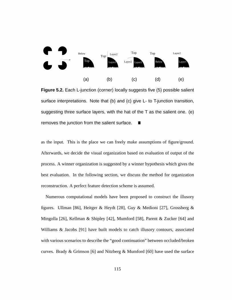
Top
Below
Layer1
Layer2Top
Layer1
Top
Layer2 Below
Top
Layer1
Layer2
(a) (b) (c) (d) (e)
Figure 5.2. Each L-junction (corner) locally suggests five (5) possible salient
surface interpretations. Note that (b) and (c) give L- to T-junction transition,
suggesting three surface layers, with the hat of the T as the salient one. (e)
removes the junction from the salient surface.
as the input. This is the place we can freely make assumptions of figure/ground.
Afterwards, we decide the visual organization based on evaluation of output of the
process. A winner organization is suggested by a winner hypothesis which gives the
best evaluation. In the following section, we discuss the method for organization
reconstruction. A perfect feature detection scheme is assumed.
Numerous computational models have been proposed to construct the illusory
figures. Ullman [86], Heitger & Heydt [28], Guy & Medioni [27], Grossberg &
Mingolla [26], Kellman & Shipley [42], Mumford [58], Parent & Zucker [64] and
Williams & Jacobs [91] have built models to catch illusory contours, associated
with various scenarios to describe the “good continuation” between occluded/broken
curves. Brady & Grimson [6] and Nitzberg & Mumford [60] have used the surface
115
reconstruction formulation to describe the salient/occluded surfaces. Besides the con-
struction of the illusory contours/surfaces, our model provides a reason to describe
why the illusory effect happens in one case instead of others by a surface/regional
description.
5.2 L-junctions and Prior Distribution of Hypotheses
The idea of picking correct visual organization is inspired by the Kanizsa square.
However, we do not perceive the similar phenomenon for another similar figure,
the four-crosses in Fig. 5.1 (b2). The key to make this difference comes from the
smooth curve preference for surface reconstruction. We consider an organization
picking scheme with such preference. In particular, on surface contours, L-junctions,
T-junctions and their interpretations will be studied.
For a given imageI, we build the bridge between sparse data and global decision
by the decay diffusion process used in Sec. 2.2. A discrete version which has been
discussed in Appendix B is examined here. We have the hypothesis choice basis
H = f1; 0; 1g ;
with 1 and1 represent foreground and background respectively and0 is the neutral
hypothesis indicating an ignorance. Each edge feature is assigned by such local
116
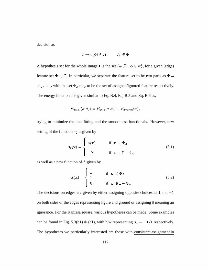
decision as
! a() 2 H : 8 2
A hypothesis set for the whole imageI is the setfa() : 2 g, for a given (edge)
feature set I. In particular, we separate the feature set to be two parts as =
A [ O with the setA=O to be the set of assigned/ignored feature respectively.
The energy functional is given similar to Eq. B.4, Eq. B.5 and Eq. B.6 as,
Edecay(j0) = Edata(j0) + Esmooth() ;
trying to minimize the data fitting and the smoothness functionals. However, new
setting of the function0 is given by
0(x) =
8>><>>:
a(x) ; if x 2 A
0 : if x 2 I A
(5.1)
as well as a new function of given by
(x) =
8>><>>:
1
; if x 2 A
0 : if x 2 I A
(5.2)
The decisions on edges are given by either assigning opposite choices as1 and1
on both sides of the edges representing figure and ground or assigning0 meaning an
ignorance. For the Kanizsa square, various hypotheses can be made. Some examples
can be found in Fig. 5.3(b1) & (c1), with b/w representing0 = 1=1 respectively.
The hypotheses we particularly interested are those with consistent assignment in
117
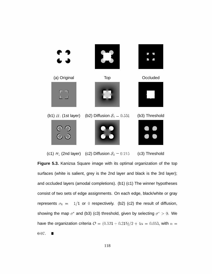
(a) Original Top Occluded
(b1) H1 (1st layer) (b2) Diffusion S1 = 0:531 (b3) Threshold
(c1) H1 (2nd layer) (c2) Diffusion S2 = 0:215 (c3) Threshold
Figure 5.3. Kanizsa Square image with its optimal organization of the top
surfaces (white is salient, grey is the 2nd layer and black is the 3rd layer);
and occluded layers (amodal completions). (b1) (c1) The winner hypotheses
consist of two sets of edge assignments. On each edge, black/white or gray
represents 0 = 1=1 or 0 respectively. (b2) (c2) the result of diffusion,
showing the map and (b3) (c3) threshold, given by selecting > 0. We
have the organization criteria O = (0:531 + 0:215)=2 + 4 = 0:653, with =
0:07.
118
neighboring edgesexcept those neighbors crossing the edges. However, we do al-
low more freedom in the assignment of junctions, by adopting the interpretations of
junctions in Fig. 5.2.
For each hypothesis set, a diffusion result can be derived, called. By the same
linear transform used in Eq. 2.12, we find the probability mapp.
Zero Energy Decay For the function(x) in Eq. 5.2, we mainly follow the choice
made in Geiger et al. [19] where the decay coefficient is chosen to be0, no energy
decay throughout our discussions and experiments in this chapter.
Modal, Amodal Completion and Multiple Surfaces
After the process, a surface is collected by those pointsx with p(x) > 0:5, called
the salient surface. Usually, scenes contain more than one surface. We will obtain all
of them by consecutively applying the above procedure. Namely, after the removal
of a surface, the “used/not ignored” featuresA where0 6= 0 will be removed
as well, and another hypothesis set can be assigned for those “not used/ignored”
featuresO = A. Multiple surfaces can be found in such manner. We have
=SS
s=1s for a S-surface reconstruction with the assigned featureA = s in
the s-th surface reconstruction. For the Kanizsa square, two surfaces (three layers,
including the background) can be formed in Fig. 5.3(b3) & (c3). The top row shows
119
the typical multiple-surface reconstruction.
Prior Distribution of Hypothesis
The prior distribution for shapes suggests smooth contours. Therefore, a favored hy-
pothesis set should be the one with more cancellation of L-junctions. That is, on L-
junctions, we assign non-zeroa() on both sides of the peak in different steps of sur-
face reconstructions. Thus the L-junctions become T-junctions, such as in Fig. 5.2(b)
or (c). We evaluate such movement by the cost
C1(fa()g) = #(L-junction! T-junction) :
Because number of L-junctions from the input is fixed, the previous criteria can be
substituted by another equivalent one as
C(fa()g) =SXs=1
#L-junctions(ps) ;
counting number of L-junctions for the resultps on the surfaces. The criteriaC and
C1 are just a constant away from each other. A smaller one gives a higher preference.
Entropy of Visible Surfaces
To give the decision for the best organization, we also compute the (normalized)
entropy for allS surfaces by
S(fa()g) = 1
S
SXs=1
1
Ns
Xx2s
ps(x) log ps(x) + (1 ps(x)) log(1 p
s(x)) ; (5.3)
120
whereNs = jsj denotes number of pixels in thes-th surfaces.
Organization Criteria
Our final organization criteria is the sum of both criteria
O(fa()g) = C(fa()g) + S(fa()g) ;
for a parameter. For instance, the hypothesis yielding the original Kanizsa image
will haveO = C(fa()g) + 0 = 12 because we have a closed-door diffusion.
The parameter balances both terms can be decided empirically by the following
experiment (Fig. 5.4).
For the Kanizsa square, one set of hypothesesH0 can be given by the original
setting, suggesting the original four pecmen as the (only) salient surfaces. Another
set of hypothesesH1, the typical hypothesis set suggests (1) a salient square and (2)
four occluded circles on the back. The human experiments suggest that for Kanizsa
images, salience of the square decreases as we move those four pecmen away from
each other as those from Fig. 5.4(a) to (c). Empirically, we can obtain the transition
point where the hypothesisH0 andH1 yield the same preference. This situation can
be described by
4 + S = 12 , = S=8 ;
whereS is the entropy value of configuration of the transition point (perception
121
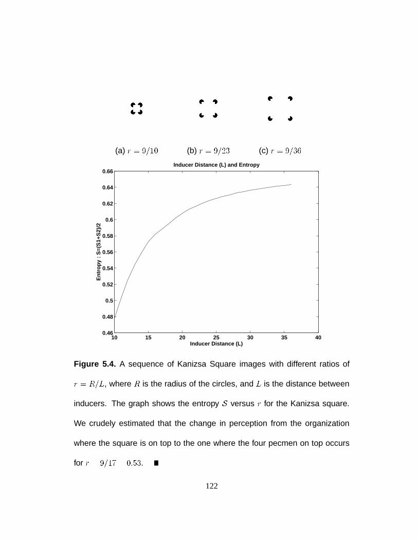
(a) r = 9=10 (b) r = 9=23 (c) r = 9=36
10 15 20 25 30 35 400.46
0.48
0.5
0.52
0.54
0.56
0.58
0.6
0.62
0.64
0.66Inducer Distance (L) and Entropy
Inducer Distance (L)
Ent
ropy
: S
=(S
1+S
2)/2
Figure 5.4. A sequence of Kanizsa Square images with different ratios of
r = R=L, where R is the radius of the circles, and L is the distance between
inducers. The graph shows the entropy S versus r for the Kanizsa square.
We crudely estimated that the change in perception from the organization
where the square is on top to the one where the four pecmen on top occurs
for r = 9=17 = 0:53.
122
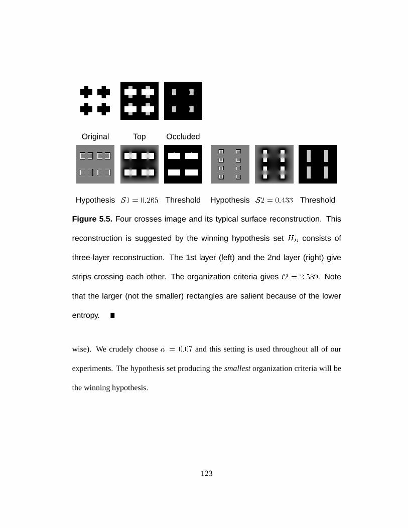
Original Top Occluded
Hypothesis S1 = 0:265 Threshold Hypothesis S2 = 0:433 Threshold
Figure 5.5. Four crosses image and its typical surface reconstruction. This
reconstruction is suggested by the winning hypothesis set HD consists of
three-layer reconstruction. The 1st layer (left) and the 2nd layer (right) give
strips crossing each other. The organization criteria gives O = 2:589. Note
that the larger (not the smaller) rectangles are salient because of the lower
entropy.
wise). We crudely choose = 0:07 and this setting is used throughout all of our
experiments. The hypothesis set producing thesmallestorganization criteria will be
the winning hypothesis.
123
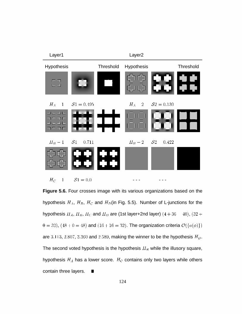
Layer1 Layer2
Hypothesis Threshold Hypothesis Threshold
HA 1 S1 = 0:495 HA 2 S2 = 0:130
HB 1 S1 = 0:711 HB 2 S2 = 0:422
HC 1 S1 = 0:0 - - - - - -
Figure 5.6. Four crosses image with its various organizations based on the
hypothesis HA, HB, HC and HD(in Fig. 5.5). Number of L-junctions for the
hypothesis HA, HB, HC and HD are (1st layer+2nd layer) (4 + 36 = 40), (32+
0 = 32), (48+ 0 = 48) and (16+ 16 = 32). The organization criteria O(fa()g)
are 3:113, 2:807, 3:360 and 2:589, making the winner to be the hypothesis HD.
The second voted hypothesis is the hypothesis HB while the illusory square,
hypothesis HA has a lower score. HC contains only two layers while others
contain three layers.
124
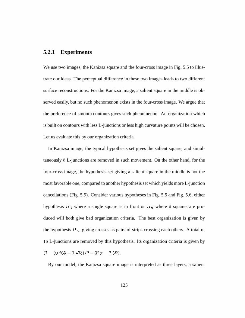
5.2.1 Experiments
We use two images, the Kanizsa square and the four-cross image in Fig. 5.5 to illus-
trate our ideas. The perceptual difference in these two images leads to two different
surface reconstructions. For the Kanizsa image, a salient square in the middle is ob-
served easily, but no such phenomenon exists in the four-cross image. We argue that
the preference of smooth contours gives such phenomenon. An organization which
is built on contours with less L-junctions or less high curvature points will be chosen.
Let us evaluate this by our organization criteria.
In Kanizsa image, the typical hypothesis set gives the salient square, and simul-
taneously8 L-junctions are removed in such movement. On the other hand, for the
four-cross image, the hypothesis set giving a salient square in the middle is not the
most favorable one, compared to another hypothesis set which yields more L-junction
cancellations (Fig. 5.5). Consider various hypotheses in Fig. 5.5 and Fig. 5.6, either
hypothesisHA where a single square is in front orHB where9 squares are pro-
duced will both give bad organization criteria. The best organization is given by
the hypothesisHD, giving crosses as pairs of strips crossing each others. A total of
16 L-junctions are removed by this hypothesis. Its organization criteria is given by
O = (0:265 + 0:433)=2 + 32 = 2:589.
By our model, the Kanizsa square image is interpreted as three layers, a salient
125
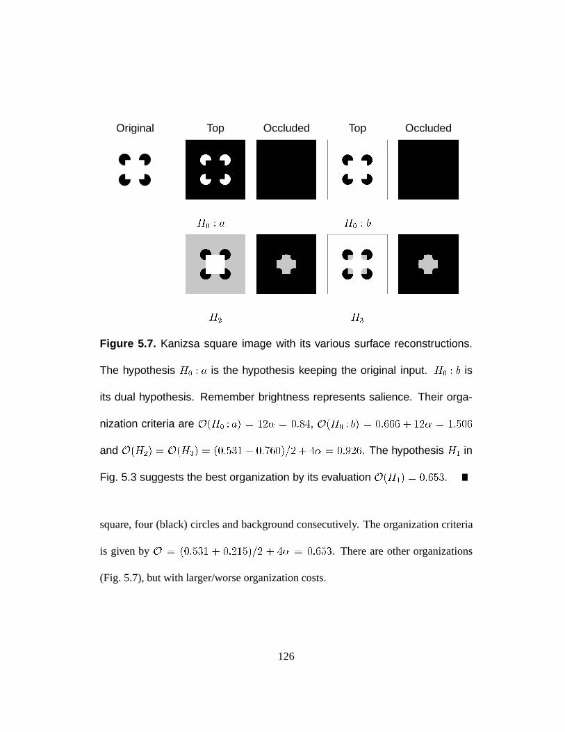
Original Top Occluded Top Occluded
H0 : a H0 : b
H2 H3
Figure 5.7. Kanizsa square image with its various surface reconstructions.
The hypothesis H0 : a is the hypothesis keeping the original input. H0 : b is
its dual hypothesis. Remember brightness represents salience. Their orga-
nization criteria are O(H0 : a) = 12 = 0:84, O(H0 : b) = 0:666 + 12 = 1:506
and O(H2) = O(H3) = (0:531 + 0:760)=2 + 4 = 0:926. The hypothesis H1 in
Fig. 5.3 suggests the best organization by its evaluation O(H1) = 0:653.
square, four (black) circles and background consecutively. The organization criteria
is given byO = (0:531 + 0:215)=2 + 4 = 0:653. There are other organizations
(Fig. 5.7), but with larger/worse organization costs.
126

5.2.2 Discussions
First of all, this approach is different from the approach by Kumaran et al. [48].
Each of their hypothesis set might produce2 dual hypothesis sets, figure/ground or
ground/figure in our set of organizations. Namely, no knowledge of F/G were consid-
ered in their context. The junction interpretations such as Fig. 5.2(a) and (d) were not
distinguished. Accordingly, while their computation of entropy is made throughout
all image space, we only compute entropy for the “visible surfaces”, i.e., points for
p > 0:5.
To speak of minors of this approach. The organization criteria contain two parts,
entropy of the visible surfaces and the cost of L-junctions. More L- to T-junction
transformations can ease the cost of organization criteria and give good organization.
Therefore, this approach is highly relies on the input from a good junction detector.
In general, we should be able to pick up junctions or high-curvature points on images
without making artificial border between them.
Let us discuss complexity of this approach. To pick the best organization, we use a
brute force search. So number of the trials is exponential to the number of junctions.
Because junctions are the only place the hypothesis can be switched, based on our
assumption that only consistent hypothesis (in neighboring points on one side of the
edges) is considered.
127

128
Chapter 6
Conclusion
We discussed the issues of figure ground separation, shape representation and per-
ceptual organization which are generally considered as low- to middle-level vision
problems. Two types of diffusion processes, the decay process and the orientation
process were defined, followed by two convexity measures. Our convexity measure-
ment was a support to the traditional1-0 convexity definition in mathematics which
separates shapes into two groups, “convex” and “concave” without any further de-
scriptions. The continuous manner in our convexity measures was established to
provide the transition from “highly convex” to “highly concave” shapes. Besides
convexity measuring, our processes were able to collect other shape information, in-
cluding symmetry and junction information.
129
Decay Diffusion Process The decay process was used in particular for simulating
the F/G phenomenon. For a F/G image, when the size of regions and the number of
inducers were normalized to be the same, we predicted the “correct” answer corre-
sponding to the outcome from the majority of human tests.
Orientation Diffusion Process For the orientation process, a wider range of im-
ages have been tested. First, it could deal with F/G images with sizes of regions
not yet normalized to be the same. A brand new design of introducing a free pa-
rameter allowed us to surf between the size-invariant convexity measuring and the
convexity measuring with the small-size preference. Other than predicting the F/G
phenomenon, the model could be considered as a definition for shape convexity. The
shapes with either similar or not similar sizes could be compared to each other, by
the choice of a small parameter. To discuss the perfectly-convex shapes which
was categorized as one group by the mathematical definition, our measure showed
the ability to distinguish between them. The study showed that the convexity mea-
sure based on the orientation process gave the scores of circles better than hexagons,
followed by squares and then triangles. Another series of experiment suggested the
preference of squares over rectangles. It could be understood as the simulation of
the Law of Pragnanz for 2-D shapes. A Kullback-Leibler distance was used as the
convexity measure.
130
Internal Shape Representation Our diffusion processes could also be used to
compute the internal shape structure, generally known as the axis study. In our ap-
proaches, two so called “shape axes” have been defined, one from the decay diffusion
and the other from the orientation diffusion. We defined two operations generating
two types of axes. For the decay process, a traveling method on the 3-D surface
S (x;(x)) was used, based on the result(x) derived from the process.
For the orientation process, a simple technique, called the local computation method
was used to collect the axes. In this case, we adopted a different point of view for
the axis finding. Instead of producing any binary axis information, we derived the
symmetry mapssym andsymM to give suggestions for shape axes. Our approach
had many benefits. First, once the diffusion process was done, the computation, via
some local operations, was easier compared to other algorithms to find the symmetry
axis. Secondly, our shape axes were computed by a global consideration. Within a
shape, we could distinguish between strong axes and weak axes. When noise, such
as protrusion were added to the boundary, our result showed a continuous transition
from ignored, having minor axes to disturbing the main structure of the shape. Also,
the junction detection was discussed. To us, the junction feature was no more than
thespecial axis point, just those happened to be on the borders. Combine with the
convexity measuring, we tried to emphasize that our simulations has the goal to cover
wide range of the applications.
131

6.1 Continuous Simulation based on Global Consid-
erations
In our simulations, based on the global considerations, we tried to remove the artifi-
cial assumptions generally used in many studies:
i For the convexity measuring, we did not draw the border between the convex
and concave shapes which was used in mathematics. Instead, we defined con-
tinuous convexity measures. They are more appropriate than the1=0 definition
in most vision applications.
ii For axis, we did not assume that the place was on or off the axes, instead, we
gave the map telling “how likely” the place was an axis point and how strong
the axis is. Therefore, we did not have to apply any additional heuristic or
non-heuristic algorithms to deal with the axis pruning or selection. The axes
generated by us had different weights themselves to guide the process.
iii For junctions, we did not distinguish between “discontinuous junctions” and
“high curvature junctions”. Instead, a map was derived and the threshold de-
cided later could be used to collect the information whatever fits to our appli-
cations.
132

6.2 Shape Description and Shape Completion
In our approach, the partial and completed shapes were treated similarly. For the
perceptual organization problem, the same framework, the decay process and entropy
measurement used for the F/G separation, was applied to select the salient shapes.
To improve the decay model used in the perceptual organization finding, we put
our future concentrations on:
i Adopt the orientation diffusion process in the perceptual organization finding.
The assumption of perfect junction detection will no longer be necessary.
ii Search for an efficient algorithm or approach to achieve the best organization.
iii Real image studies.
133

134
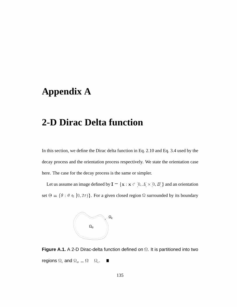
Appendix A
2-D Dirac Delta function
In this section, we define the Dirac delta function in Eq. 2.10 and Eq. 3.4 used by the
decay process and the orientation process respectively. We state the orientation case
here. The case for the decay process is the same or simpler.
Let us assume an image defined byI fx : x 2 [0; A][0; B]g and an orientation
set f : 2 [0; 2)g. For a given closed region surrounded by its boundary
Ωα
Ωε
Figure A.1. A 2-D Dirac-delta function defined on . It is partitioned into two
regions and .
135
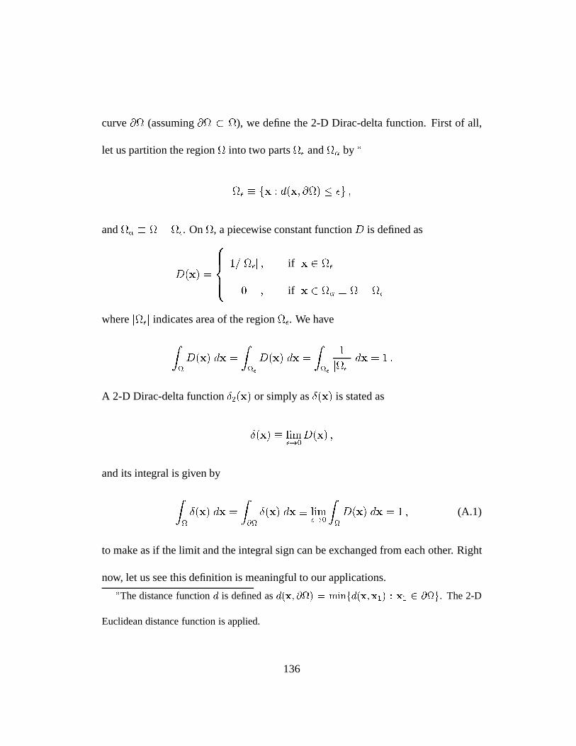
curve@ (assuming@ ), we define the 2-D Dirac-delta function. First of all,
let us partition the region into two parts and by
fx : d(x; @) g ;
and . On, a piecewise constant functionD is defined as
D(x) =
8>><>>:
1=jj ; if x 2
0 ; if x 2
wherejj indicates area of the region. We have
Z
D(x) dx =
Z
D(x) dx =
Z
1
jjdx = 1 :
A 2-D Dirac-delta functionÆ2(x) or simply asÆ(x) is stated as
Æ(x) lim!0
D(x) ;
and its integral is given by
Z
Æ(x) dx =
Z@
Æ(x) dx lim!0
Z
D(x) dx = 1 ; (A.1)
to make as if the limit and the integral sign can be exchanged from each other. Right
now, let us see this definition is meaningful to our applications.The distance functiond is defined asd(x; @) = minfd(x;x1) : x1 2 @g. The 2-D
Euclidean distance function is applied.
136
For a binary input, an intensity functionI characterizing, we define the hypoth-
esis function0(x; ) as
0(x; ) =
8>><>>:
u n if u n 0 ^ x 2 @
0 if u n < 0 _ x 2 @
and based on it, a function(x; ) is defined by
(x; ) =
8>><>>:
0(x; ) Æ(x) if u n 0 ^ x 2 @
if u n < 0 _ x 2 @
The operation “ ” denotes the conventional inner product inR2. The vectoru and
n(x) respectively denote the unit vector(cos ; sin ) and the unit inward normal on
x 2 @. For the case that a smooth intensity functionI(x) is available, we can define
0(x; ) as
(x; ) =
8>><>>:
1Me
@I(x)@u
Æ(x) if x 2 @
if x 2 @
The constantMe is defined bymaxfj@I(x)@u
j : x 2 I; 2 g, evaluated on a compact
set. In either case, we would like to discuss the integral of(x; ) on, for two
parts@ and( @) . The inside part is
Z(@)
(x; ) dx d = 2jj : (A.2)
The “border part” can be estimated by
Z@
(x; ) dx d
Z 2
0
Z@
1 Æ(x) dx d =
Z 2
0
1 d = 2; (A.3)
137
which gives an upper bound of the integral. Furthermore, let us assume, at each
pointx of the curve@, the normal direction to the curve@ is always the gradient
direction of the intensity functionI at pointx. The lower bound of the integral can
be given as by
Z@
(x; ) dx d
Z@
Z 2
2
mg cos Æ(x) d dx
= mg
Z@
2Æ(x) dx = 2mg ; (A.4)
givenmg = minfkrI(x)k=Me : x 2 @g, the (normalized) minimal value of
length of the gradient vectors on the boundary@. We can assumemg > 0. It gives
0 <R@
(x; ) dx d 2. Therefore it is meaningful to include the data-fitting
integral in our variational functionals, as in Eq. 2.9 and Eq. 3.6.
138
Appendix B
Decay Diffusion Process, Random
Walk and Discrete Settings
To write down the discrete form of the energy functional either Eq. 2.9 or Eq.2.9,
first, let us discretize the information and represent the input data0, the function
and the diffusion field as column vectors by the raster scanning order. That is,
for anM N image as an index setI fk = 1; ; K = N Mg containing the
shape, the input vector is given by0(k) : I ! f1; 0; 1g and the function is
(k) : I ! f; 1=g for a small constant called delta function coefficientwhereThe conversation in this section will deal with the most general case happened in our
text. It covers discussions for Sec. 2.2 and Chapter 5. Also, we will continue to use the same
set of notations here in discrete case.
139
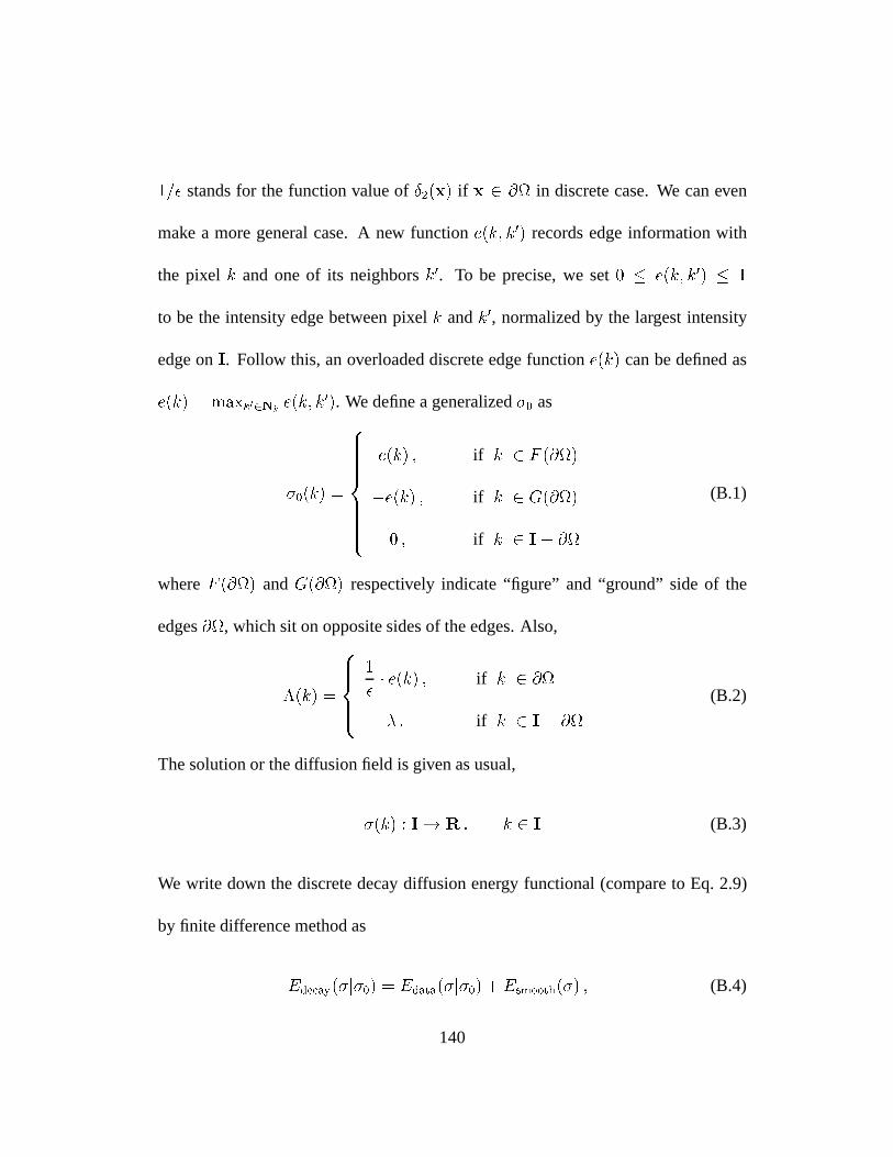
1= stands for the function value ofÆ2(x) if x 2 @ in discrete case. We can even
make a more general case. A new functione(k; k0) records edge information with
the pixelk and one of its neighborsk0. To be precise, we set0 e(k; k0) 1
to be the intensity edge between pixelk andk0, normalized by the largest intensity
edge onI. Follow this, an overloaded discrete edge functione(k) can be defined as
e(k) = maxk02Nke(k; k0). We define a generalized0 as
0(k) =
8>>>>>><>>>>>>:
e(k) ; if k 2 F (@)
e(k) ; if k 2 G(@)
0 ; if k 2 I @
(B.1)
whereF (@) andG(@) respectively indicate “figure” and “ground” side of the
edges@, which sit on opposite sides of the edges. Also,
(k) =
8>><>>:
1
e(k) ; if k 2 @
: if k 2 I @
(B.2)
The solution or the diffusion field is given as usual,
(k) : I! R : k 2 I (B.3)
We write down the discrete decay diffusion energy functional (compare to Eq. 2.9)
by finite difference method as
Edecay(j0) = Edata(j0) + Esmooth() ; (B.4)
140
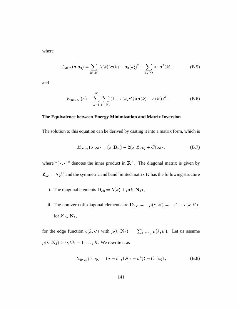
where
Edata(j0) =Xk2@
(k)((k) 0(k))2 +
Xk 62@
2(k) ; (B.5)
and
Esmooth() =KXk=1
Xk02Nk
(1 e(k; k0))((k) (k0))2: (B.6)
The Equivalence between Energy Minimization and Matrix Inversion
The solution to this equation can be derived by casting it into a matrix form, which is
Edecay(j0) = (;D) 2(;L0) + C(0) : (B.7)
where “( , )” denotes the inner product inRK. The diagonal matrix is given by
Lkk = (k) and the symmetric and band limited matrixD has the following structure
i. The diagonal elementsDkk = (k) + (k;Nk) ,
ii. The non-zero off-diagonal elements areDkk0 = (k; k0) = (1 e(k; k0))
for k0 2 Nk,
for the edge functione(k; k0) with (k;Nk) =P
k02Nk(k; k0). Let us assume
(k;Nk) > 0, 8k = 1; : : : ; K. We rewrite it as
Edecay(j0) = ( ;D( )) + C1(0) ; (B.8)
141
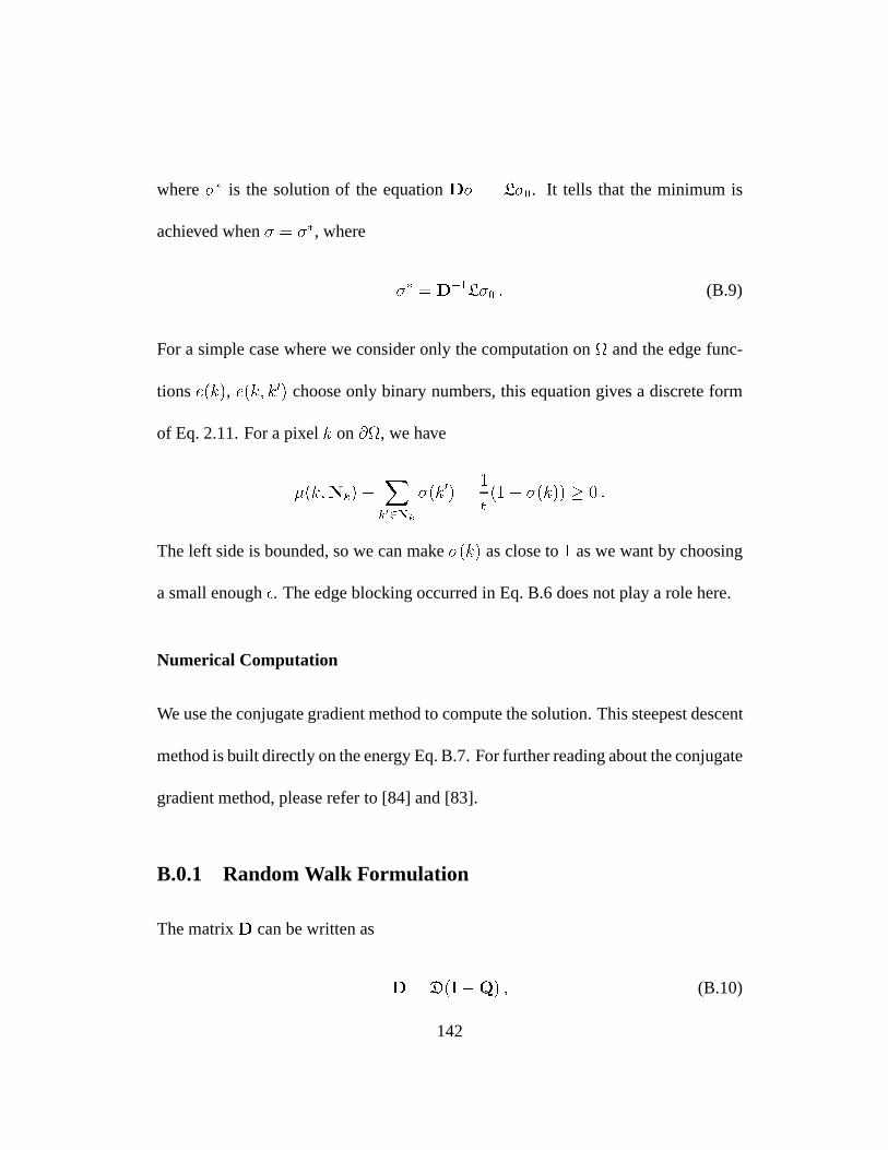
where is the solution of the equationD = L0. It tells that the minimum is
achieved when = , where
= D1L0 : (B.9)
For a simple case where we consider only the computation on and the edge func-
tionse(k), e(k; k0) choose only binary numbers, this equation gives a discrete form
of Eq. 2.11. For a pixelk on@, we have
(k;Nk)Xk02Nk
(k0) =1
(1 (k)) 0 :
The left side is bounded, so we can make(k) as close to1 as we want by choosing
a small enough. The edge blocking occurred in Eq. B.6 does not play a role here.
Numerical Computation
We use the conjugate gradient method to compute the solution. This steepest descent
method is built directly on the energy Eq. B.7. For further reading about the conjugate
gradient method, please refer to [84] and [83].
B.0.1 Random Walk Formulation
The matrixD can be written as
D = D(IQ) ; (B.10)
142
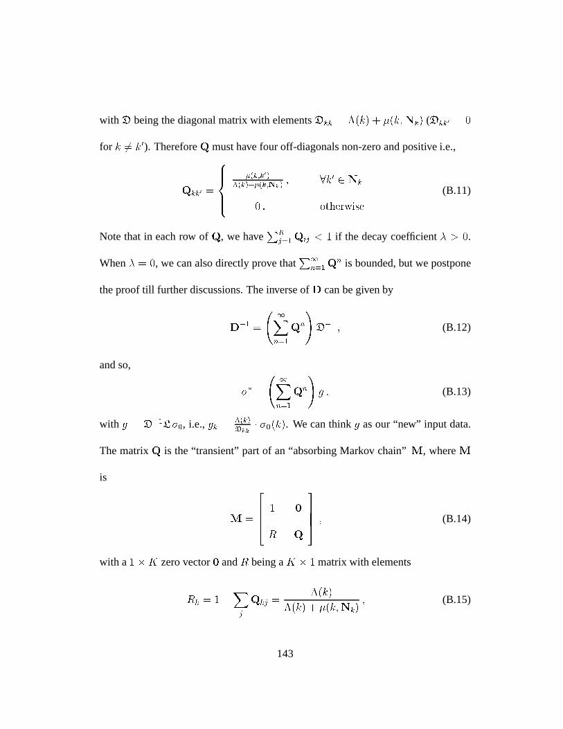
with D being the diagonal matrix with elementsDkk = (k) + (k;Nk) (Dkk0 = 0
for k 6= k0). ThereforeQ must have four off-diagonals non-zero and positive i.e.,
Qkk0 =
8>><>>:
(k;k0)(k)+(k;Nk)
; 8k0 2 Nk
0 : otherwise
(B.11)
Note that in each row ofQ, we havePK
j=1Qij < 1 if the decay coefficient > 0.
When = 0, we can also directly prove thatP1
n=1Qn is bounded, but we postpone
the proof till further discussions. The inverse ofD can be given by
D1 =
1Xn=1
Qn
!D1 ; (B.12)
and so,
=
1Xn=1
Qn
!g ; (B.13)
with g = D1L 0, i.e.,gk =(k)Dkk
0(k). We can thinkg as our “new” input data.
The matrixQ is the “transient” part of an “absorbing Markov chain”M, whereM
is
M =
2664 1 0
R Q
3775 ; (B.14)
with a1K zero vector0 andR being aK 1 matrix with elements
Rk = 1Xj
Qkj =(k)
(k) + (k;Nk); (B.15)
143
so thatPK+1
j=0 Mij = 1, 8i. The stochastic matrixM is of sizeK + 1 byK + 1. It is
clear that
Mn =
2664 1 0
R0 Qn
3775 ;
whereR0 =Pn
=0QR. M is an absorbing Markov chain in the sense that if one
starts with any states0, by successively applyingM, one ends up in the statesnal =
(1; 0; 0; :::; 0), i.e., snal = limn!1 s0Mn (we are applying the matrix to the vector
to the “left”). This is clear from the fact thatlimn!1Qn = 0. This is whyQ is the
transient part ofM. The interpretation of the states = (1; 0; :::; 0), is of “death” of
the random walk, since the random walk jumped to the zero-th coordinate that is not
a pixel in the lattice. Moreover, once it reaches the zero-th coordinate it never leaves,
i.e., s = (1; 0; 0; ::::; 0) is an eigenstate ofM or sM = s (or equivalently, to the
“right” sT is an eigenstate ofMT , withMT sT = sT . This is the absorbing state.
Random Walk View
Let us clarify the random walk interpretation of the matrices.
(Qn)kj- probability that a random walk that started at pixelk will reach pixel
j in then-th step.
Rk- probability that a random walk will vanish at pixelk (move to the zero-th
state coordinate).
144
R0k = (
Pn
=0QR)
k- probability that the random walk vanished at pixelk in
n steps.
(P1
n=1Qn)k;j-probability that the random walk started at pixelk and reached
pixel j in any number of steps.
The last statement gives a reason whyPn
k=1Qn is bounded no matter is 0 or not.
To speak of the random walk interpretation, in one step, for example, the random
walk starting atk has probability non-zero,Qk;j =(k;j)
(k)+(k;Nk), to move to one of its
j 2 Nk neighbors and with probabilityRk =(k)
(k)+(k;Nk)to be vanished. A random
walk path is a path which starts from the pixelk, travels around the image, ends up a
pixel j and vanishes there with probabilityRj. Thus, we conclude this section with
the random walk view interpretation of the solution (Eq. B.9 or Eq. B.13) :
The solution(k) corresponds to the expected value of0 at the first vanishing
point of the random walk starting at the pixelk.
The vanishing point can be either on the boundaries@ or not on the boundary. The
probability of one pathWk starting atk, going throughk = k0; : : : ; kn and vanishes
atkn can be written as
P(Wk) = Rkn
n1Yi=0
Qki;ki+1 = Rkn
n1Yi=0
(ki; ki+1)
(ki) + (ki; Nki): (B.16)
Usually, for the simple case wheree(k), e(k; k0) take only binary numbers, we can
expect that once a particle reach@, it is likely to be vanished there if we choose
145
small enough to make the vanish probabilityRk = 1=(1 + (k;Nk)), k 2 @ as
close to1 as we want. Thus, we can provide a simpler form forP(Wk) as
P(Wk) = Rkn
n1Yi=0
Qki;ki+1 n1Yi=0
Qki;ki+1 = (+ 4)n ; (B.17)
if the path touch boundary only once and vanishes there atkn. Under this approx-
imation, with or without edge blocking is no longer an issue. All the paths touch
boundaries more than once can simply be ignored as truncation of higher order terms,
compared to previous type walks. For other paths stopy atk 2 I@, i.e., the paths
never reach any part of the boundary, we have
P(Wk) = Rkn
n1Yi=0
Qki;ki+1 =
+ 4(+ 4)n : (B.18)
Keep remember that a smaller provides less decay.
Let us run all the paths backward, and consider only the path starting from@, we
can write another version of interpretation for:
The solution(k) correspond to the summation of probability of multiple source
random walks, where each random walk starts from a boundary pixeli 2 @ and
arrives (not “stops”) atk. The walk carries the weightgi =(i)
(i)+(i;Ni) 0(i) or
yFor random walks, we will use “stops” and “arrives” at certain location to specify
whether we need to multiply the vanishing probability which only applied to the case of
stopped walks.
146
for a simpler case asgi =1
1+(i;Ni)from a pixeli 2 @ (i.e., corners tend to weight
more).
When both sides andI are considered simutaneously, the weight carried by
those random walks can be either positive or negative depends on the sign of0. The
calculation is therefore done by summing all those “signed probability”. Here the
summation cares only the walks starting from a boundary pixelk 2 @. I.e., for the
simple case wheree(k), e(k; k0) take only binary values, under this interpretation,
we need to consider only those paths as in Eq. B.17 and paths as in Eq. B.18 can be
ignored, if we choose a small enough.
Probability Interpretation
For the last two interpretations, we consider the solution as an expectation or a sum-
mation. It is interesting to view the result as a probability distribution. To see this,
we need a linear transform from to p by
p(k) =1
2(1 + (k)) ;
as we have used in Eq. 2.12. Let us discuss the case with = 0 first, withp0(k) being
either1 or 0 for k 2 @ (i.e., the inducers0(k) = 1 / 1), assuminge(k) = 1,
8k 2 @. Again, we assume that the walk hitting boundaries more than once will
vanish very likely and can be ignored. Therefore, the solutionp, similar to, is an
147
expectation and can be written as
p(k) = 1 X
i2F (@);t
P(W (t) = i; stops ati jW (0) = k)
+ 0 X
i2G(@);t
P(W (t) = i; stops ati j W (0) = k)
X
i2F (@);t
P(W (t) = i; stops ati and visits@ for the first time jW (0) = k)
= P(W visitsF (@) before it visitsG(@) jW (0) = k) (B.19)
asF (@) andG(@) indicating “figure” and “ground” side of the edges@. We
can makep(k) as close to the probabilityP(Wk visitsF (@) beforeG(@)) as we
want, if we choose small enough,
When the decay coefficient is not zero, we have an extra term
1
2X
i2@;t
P(W (t) = i; stops ati without touching@ jW (0) = k) :
It is for the case where a walk stops at interior pixelsi 2 @. We can say
that for half of the chance, the location will be figure and will be background for the
other half of the chance, for it lacks of knowledge to commit. The same probability
interpretation forp that we just described can stand still. We conclude it as
The solution0 p(k) 1, derived by a linear transformation from1 (k)
1, is an approximation to the probabilityP(Wk visitsF (@) before it visitsG(@)).
The approximation can be as good as we want, if a small enough is provided.
This interpretation suggests us to use the entropy criteria to measure the shape con-
148
vexity, as we described in Sec. 2.2.2 or Eq. 2.12 & Eq. 2.13.
B.1 Decay Process and Convexity
Let us examine why our model can catch convexity. We will check the example
in Fig. B.1 where the regionsa andb = I a share a common boundary.
A simpler version of the energy functional in Eq. B.4 wheree(k) ande(k; k0) take
only binary numbers will be discussed. For pixelsp andq, we usepq to indicate the
Euclidean distance between them. The shortest legal path betweenp andq within the
shapea (orb) is indicated byda(p; q) (or db(p; q)).
In Fig. B.1, given a source pixelp (along the boundary) and given a pixelq at the
convex side of the figure, there is a pixelq0 equally distant top (Euclidean distance)
in the concave side (There are many pixelsq0 with such property). In the concave
region the shortest legal walk betweenp and q0 traverse a distanced(p; q0) > pq0
while in the convex region, the shortest legal walk betweenp andq always traverse a
distanced(p; q) = pq = pq0.
By the result of random walk in last section, the contribution to the the final so-
lution (q) and(q0) of the sourcep to q andq0 is directly dependent ond(p; q)
andd(p; q0) respectively. This is because with the decay term, only the pixels with
shorter distance can be reached by the random walk. The longer is the path to reach
149
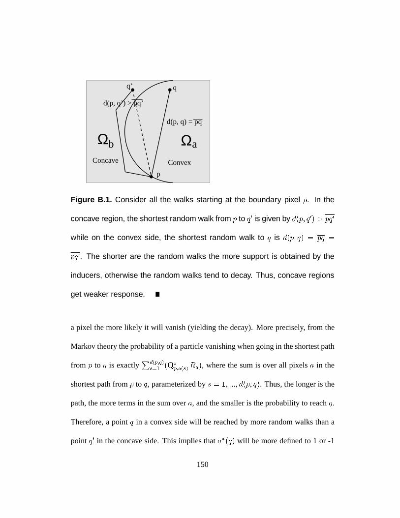
d(p, q) = pq
d(p, q’) > pq’
Concave
p
q’ q
Convex
bΩ aΩ
Figure B.1. Consider all the walks starting at the boundary pixel p. In the
concave region, the shortest random walk from p to q0 is given by d(p; q0) > pq0
while on the convex side, the shortest random walk to q is d(p; q) = pq =
pq0. The shorter are the random walks the more support is obtained by the
inducers, otherwise the random walks tend to decay. Thus, concave regions
get weaker response.
a pixel the more likely it will vanish (yielding the decay). More precisely, from the
Markov theory the probability of a particle vanishing when going in the shortest path
from p to q is exactlyPd(p;q)
s=1 (Qsp;a(s)Ra), where the sum is over all pixelsa in the
shortest path fromp to q, parameterized bys = 1; :::; d(p; q). Thus, the longer is the
path, the more terms in the sum overa, and the smaller is the probability to reachq.
Therefore, a pointq in a convex side will be reached by more random walks than a
point q0 in the concave side. This implies that(q) will be more defined to 1 or -1
150

(to figure or ground) than(q0) and the entropy will satisfyS(q) < S(q0). Thus,
convexity is encouraged by the entropy criteria.
151

152

Bibliography
[1] E. Adelson and P. Anandan. “Ordinal characteristics of transparency”,Proc.
AAAI Workshop on Qualitative Vision, pp. 552–573, CA, 1990.
[2] J. W. Bacus and E. E. Gose. “Leukocyte pattern recognition”,IEEE Trans. on
Systems, Man, Cybernetics, SMC-2(4), pp. 513–526, 1972.
[3] A. Blake and A. Zisserman.Visual Reconstruction, MIT Press, Cambridge,
MA, U.S.A., 1987.
[4] H. Blum. “Biological shape and visual science (part I)”,J. of Theoretical
Biology, 38: pp. 205–287, 1973.
[5] H. Blum. “A Transformation for Extracting New Descriptors of Shape”,Sym-
posium Models for Speech and Visual Form, Weiant Whaten-Dunn (ed.) Cam-
bridge, MA: MIT Press. 1967
153

[6] M. Brady and W. E. L. Grimson. “The perception of subjective surfaces”A. I.
Memo, 666, AI Lab., MIT, 1982.
[7] E. Bribiesca. “Measuring 2D Shape Compactness using the Contact Perimeter”,
Computers and Mathematics with Applications, 33(11): pp. 1–9, 1997.
[8] V. Bruce, P. R. Green and M. A. Georgeson.Visual Perception, Physiology,
Psychology, and Ecology(3rd ed.), Psychology Press, 1996.
[9] J. B. Burns, R. S. Weiss and E. M. Riseman. “The non-existence of general-case
view-invariants”, J. L. Mundy and A. Zisserman (eds.),Geometric Invariance
in Computer Vision, pp. 120–131, 1992.
[10] M. Cooper. Visual Occlusion and the Interpretation of Ambiguous Pictures,
Ellis Horwood Limited, 1992.
[11] T. M. Cover and J. A. Thomas.Elements of Information Theory, John Wiley &
Sons, 1991.
[12] R. O. Duda and P. E. Hart.Pattern Classification and Scene Analysis, John
Wiley & Sons, June 1973.
[13] J. Elder and S. W. Zucker. “Computing contour closure”,Proc. Euro. Conf.
Comp. Vis., pp. 399–412, June, 1994.
154
[14] J. Elder and S. W. Zucker. “A measure of Closure”,Vis. Res., 34(24): pp. 3361–
3369, 1994.
[15] J. Elder and S. W. Zucker. “The effect of contour closure on the rapid discrimi-
nation of two-dimensional shapes”,Vis. Res., 33: pp. 981–991, 1993.
[16] L. Euler. Methodus inveniendi lineas curvas maximi minimive proprietate gau-
dentes, Lausanne, 1744.
[17] M. Gaafar. “Convexity verification, block-chords, and digital straight lines”,
Comp. Graphics and Image Processing, 6: pp. 361–370, 1977.
[18] M. Gage and R. Hamilton. “The heat equation shrinking convex plane curves”,
J. Diff. Geom., 23: pp. 69–96, 1986.
[19] D. Geiger, H. Pao and N. Rubin. “Salient and Multiple Illusory Surfaces”,
Computer Vision and Pattern Recognition, June. 1998.
[20] D. Geiger and A. Yuille. “A common framework for image segmentation”,Int’l
J. of Comp. Vis., 6(3): pp. 227–243, 1991.
[21] S. Geman, D. Geman. “Stochastic relaxation, gibbs distributions, and the
Bayesian restoration of images”,IEEE Trans. PAMI1984.
155
[22] M. Grayson. “The heat equation shrinks embedded plane curves to round
points”, J. Diff. Geom., 26: pp. 285–314, 1987.
[23] J. E. Green.IEEE Conference Records. Symposium on Feature Extraction and
Selection in Pattern Recognition, (Argonne, IL), pp. 100–109, IEEE: New York,
1970.
[24] G. R. Grimmett and D. R. Stirzaker.Probability and Random Processes, Oxford
Science Publications, 2nd ed., 1992.
[25] W. E. L. Grimson. “The combinatorics of heuristic search termination for ob-
ject recognition in cluttered environment”,Proc. 1st Euro. Conf. Comput. Vis.,
pp. 552–556, 1990.
[26] S. Grossberg and E. Mingolla. “Neural dynamics of perceptual grouping: tex-
tures, boundaries and emergent segmentations”,Perception & Psychophysics,
38(2): pp. 141–170, 1985.
[27] G. Guy and G. Medioni. “Inferring global perceptual contours from local fea-
tures”, Proc. IU Workshop DARPA, Sept. 1992.
[28] F. Heitger and R. von der Heydt. “A computational model of neural contour
processing: Figure–ground segregation and illusory contours”,Proc. of the
IEEE, pp. 32–40, 1993.
156

[29] A. Held and K. Abe. “On the decomposition of binary shapes into meaningful
parts”, Pattern Recognition, 27(5): pp. 637–647, 1994.
[30] R. von der Heydt, E. Peterhans and G. Baumgartner. “Neuronal responses to
illusory contour stimuli reveal stages of visual cortical processing”,Visual Neu-
rosc., Cambridge: Cambridge University Press, pp. 343–351.1986.
[31] R. von der Heydt, E. Peterhans and G. baumgartner. “Illusory contours and
cortical neuron responses”,Science, 224: pp. 1260–1262, 1984.
[32] D. A. Huffman. “A duality concept for the analysis of polyhedral scenes”,
Machine Intelligence, 6, Edinb. Univ. Press, Edinb., U.K., 1971.
[33] D. D. Huffman and W. Richard. “Representing smooth plane curves for recogni-
tion: Implementations for figure-ground reversal”, Proceedings of the National
Conf. of the America Association for Artificial Intelligence (Los Altos, CA: W
Kaufmann): pp 5–8, 1982.
[34] D. D. Huffman and W. Richard. “Parts of recognition”, Cognition,18: pp 65–
96, 1984.
[35] D. Huttenlocher and P. Wayner. “Finding convex edge groupings in an image”,
Int’l J. of Comp. Vis., 8(1): pp. 7–29, 1992.
157

[36] D. W. Jacobs. “Robust and efficient detection of convex groups”IEEE Trans.
PAMI, 1995.
[37] S. Ito. Diffusion Equations, American Mathematical Society, 1992.
[38] I. H. Jermyn and H. Ishikawa. “Global optimal regions and boundaries”,Int’l
Conf. on Comp. Vis., pp. 904–910, Sep. 1999.
[39] G. Kanizsa. Organization in Vision, Essays on Gestalt Perception, Praeger,
1979.
[40] G. Kanizsa and W. Gerbino. “Convexity and symmetry in figure-ground orga-
nization”, Vision and Artifact, M. Henle (ed.), New York: Springer, 1976.
[41] M. Kass, A. Witkin, D. Terzopoulos. “Snakes: active contour models”,Int’l J.
of Comp. Vis., pp. 321–331, 1988.
[42] P. J. Kellman and T. F. Shipley. “A theory of visual interpolation in object
perception”,Cognitive Psychology, 23: pp. 141–221, 1995.
[43] C. E. Kim and A. Rosenfeld. “Digital straight lines and convexity of digital
regions”, IEEE Trans. PAMI, 4: pp. 149–153, 1982.
158
[44] B. Kimia, A. Tannenbaum, S. Zucker. “Shapes, shocks, and deformations I: the
components of two-dimensional shape and the reaction-diffusion space”,Int’l
J. of Comp. Vis., 1: pp. 189–224, 1995.
[45] K. Koffka. Principles of Gestalt Psychology, New York: Harcourst Brace,
1935.
[46] W. Kohler. Gestault Psychology: An Introduction to New Concepts in Modern
Psychology(rev. ed.), New York: Liveright, 1947.
[47] I. Kovacs and B. Julesz. “A closed curve is much more than an incomplete one:
effect of closure in figure-ground segmentation”,Proc. Natl. Acad. Sci. USA,
90: pp. 7495–7497, 1993.
[48] K. Kumaran, D. Geiger and L. Gurvits. “Illusory surfaces and visual organiza-
tion”, Network: Comput. in Neural Syst., 7:(1) pp. 33–60, Feb. 1996.
[49] A. Leaci and S. Solimini. “Variational problems with a free discontinuity set”,
Bart M. ter Haar Romeny (ed.),Geometry-Driven Diffusion in Computer Vision,
pp. 147–154, 1994.
[50] T. Leung and J. Malik. “Contour continuity in region based image segmenta-
tion”, Euro. Conf. Comp. Vis., pp. 544–559, 1998.
159
[51] T.-L. Liu and D. Geiger. “Approximate Tree Matching and Shape Similarity”,
Proc. IEEE Intl. Conference on Computer Vision, 1: pp: 456–462, 1999.
[52] T-L. Liu, D. Geiger and R. V. Kohn. “Representation and self-similarity of
shapes”,Int’l Conf. on Comp. Vis., pp. 1129–1135, 1998.
[53] Z. Liu, D. W. Jacobs and R. Basri. “The role of convexity in perceptual comple-
tion: beyond good continuation”,Vision Research, 39: pp. 4244–4257, 1999.
[54] S. Loncaric. “A survey of shape analysis techniques”,Pattern Recognition,
31(8): pp. 983–1001, 1998.
[55] S. Mallat.a Wavelet Tour of Signal Processing, Academic Press, 1998.
[56] D. Marr. Vision, New York: Freeman, 1982.
[57] D. Mumford. “Mathematical theories of shape: Do they model perception”,
Conf. Geom. Meth. In Comp. Vis., SPIE Proceedings Series, 1570: pp. 2–10,
1991.
[58] D. Mumford. “Elastica and computer vision”, C. L. Bajaj (ed.),Algebraic
Geometry and Its Applications: pp. 491–506, Springer-Verlag, New York, 1994.
160
[59] K. Nakayama, Z. J. He, S. Shimojo, “Visual surface representation: a critical
link between lower-level and higher-level vision”, S. M. Kosslyn and D. N. Os-
herson (eds.),Visual Cognition, Cambridge, MA: MIT Press, pp. 1–70, 1995.
[60] M. Nitzberg and D. Mumford. “The 2.1-D Sketch”,IEEE Int’l Conf. on Comp.
Vis., pp. 138–144, Osaka, Dec. 1990.
[61] M. Nitzberg, D. Mumford and T. Shiota.Filtering, Segmentation, and Depth,
Berlin: Springer, 1993.
[62] B. Øksendal.Stochastic Differential Equations, An Introduction with Applica-
tions, Spring-Verlag, 1989.
[63] H. Pao, D. Geiger and N. Rubin. “Measuring convexity for figure/ground sepa-
ration”, Int’l Conf. on Comp. Vis., pp. 948–955, Sep. 1999.
[64] S. Parent and S. W. Zucker. “Trace inference, curvature consistency and curve
detection”,IEEE PAMI, 11(8): pp. 823–839, 1989.
[65] G. Parisi.Statistical Field Theory, Addison-Wesley, 1988.
[66] P. Perona and J. Malik. “Scale space and edge detection using anisotropic dif-
fusion”, IEEE Trans. Pattern Anal. Mach. Intell., 12, pp. 629–639, 1990.
161
[67] D. L. Ringach and R. Shapley. “Spatial and temporal properties of illusory
contours and amodal boundary completion”,Vision Research, 36: pp. 3037–
3050, 1996.
[68] L. C. G. Rogers and D. Williams.Diffusions, Markov Processes, and Martin-
gales, 1 (2nd ed.), John Wiley & Sons, 1994.
[69] A. Rosenfeld. “Compact figures in digital pictures”,IEEE Trans. on Systems,
Man, Cybernetics, SMC-4, pp. 221–223, 1974.
[70] P. L. Rosin. “Shape Partitioning by Convexity”,IEEE Trans. Systems, Man,
and Cybernetics, part A, 30(2): pp. 202–210, 2000.
[71] E. Rubin.Visuell wahrgenommene Figuren, Copenhagen: Gyldendals, 1921.
[72] N. Rubin, K. Nakayama and R. Shapley. “Enhanced perception of illusory
contours in the lower versus upper visual hemifields”,Science, 271: pp. 651–
653, 1996
[73] J. A. Sethian.Level Set Methods, Evolving Interfaces in Geometry, Fluid Me-
chanics, Computer Vision, and Materials Science, Cambridge, 1996
[74] A. Shashua and S. Ullman. “Structural saliency: The detection of globally
salient structures using a locally connected network”,Int’l Conf. Comp. Vis.,
pp. 321–327, 1988.
162
[75] L. G. Shapiro and R. M. Haralick. “Decomposition of two-dimentional shapes
by graph-theoretic clustering”,IEEE Trans. PAMI, 1(1): pp. 10–20, 1979.
[76] R. Shapley and J. Gordon. “The existence of interpolated illusory contours
depends on contrast and spatial separation”, S. Petry and G. E. Meyer (eds.),
The Perception of Illusory Contours, Springer-Verlag, pp. 109–115, 1987.
[77] R. Shepard.Mind Sights, W. H. Freeman and Co., NY, 1990
[78] J. Shi and J. Malik. “Normalized cuts and image segmentation”,IEEE Conf.
Comp. Vis. and Pat. Rec., Puerto Rico, June 1997.
[79] F. Shumann. “Einige beobachtungen uber die zusammenfassung von gesicht-
seindrucken zu einheiten”,Physiologische Studien, 1: pp. 1–6, 1904.
[80] K. Siddiqi and B. Kimia. “A shock grammar for recognition”,Computer Vision
and Pattern Recognition, 1996.
[81] J. Sklansky. “Recognition of convex blobs”,Pattern Recognition, 2: pp. 3–10,
1970.
[82] K. A. Stevens, A. Brookes. “The concave cusp as a determiner of figure-
ground”, Perception, 17: pp. 35–42, 1988.
163
[83] J. Stoer and R. Bulirsch.Introduction to numerical analysis, translated by
R. Bartels, W. Gautschi, and C. Witzgall (2nd ed.), New York : Springer-Verlag,
1993.
[84] J. C. Strikwerda.Finite Difference Schemes and Partial Differential Equations,
Wadsworth & Brooks/Cole, 1989.
[85] B. Tang, G. Sapiro and V. Caselles. “Direction Diffusion”,Int’l Conf. on Comp.
Vis., Sep. 1999.
[86] S. Ullman. “Filling in the gaps: the shape of subjective contours and a model
for their generation”,Biological Cybernetics, 25: pp. 1–6, 1976.
[87] K. Voss.Discrete Images, Objects, and Functions inZn, Springer-Verlag, 1993.
[88] J. Weickert. “A Review of Nonlinear Diffusion Filtering”, B. ter Haar Romeny,
L. Florack, J. Koenderink, M. Viergever (eds.),Scale-Space Theory in Com-
puter Vision, Lecture Notes in Computer Science, Springer, Berlin,1252: pp. 3–
28, 1997.
[89] Y. Weiss. “Interpreting images by propagating Bayesian beliefs”, M. Mozer,
M. Jordan and T. Petsche (eds.),Advances in Neural Information Processing
System, 9: pp. 908–915, 1997.
164
[90] M. Wertheimer. Untersuchungen zur Lehre von der Gestalt, II.Psychologische
Forschung, 4: pp. 301–350. Translated as “Laws of organisation in perceptual
forms” in W. D. Ellis (1955),A source book of Gestalt psychology, London:
Routledge and Kegan Paul, 1923.
[91] L. R. Williams and D. W. Jacobs. “Stochastic completion fields: a neural model
of contour shape and salience”,Neural Computation, 9: pp. 849–870, 1997.
[92] A. P. Witkin and J. M. Tenenbaum. “On the role of structure in vision”, J. Beck,
B. Hope and A. Rosenfeld (eds.),Human and Machine Vision, 1981.
[93] I. Young, J. Walker and J. Bowie. “An Analysis technique for biological shape”,
Information and Control, 25: pp. 357–370, 1974.
165


