A Condensed Review of Nuclear Reactor Thermal … Condensed Review of Nuclear Reactor...
138
A Condensed Review of Nuclear Reactor Thermal-Hydraulic Computer Codes for Two-Phase Flow Analysis by M. Kazimi* and M. Massoud Energy Laboratory Report No. MIT-EL 79-018 February 1980 *Associate Professor, Department of Nuclear Engineering
Transcript of A Condensed Review of Nuclear Reactor Thermal … Condensed Review of Nuclear Reactor...

A Condensed Review of Nuclear ReactorThermal-Hydraulic Computer Codes
for Two-Phase Flow Analysis
by
M. Kazimi* and M. Massoud
Energy Laboratory Report No. MIT-EL 79-018February 1980
*Associate Professor, Department of Nuclear Engineering

x\
A CONDENSED REVIEW OF NUCLEAR
REACTOR THERMAL-HYDRAULIC COMPUTER CODES
FOR TWO-PHASE FLOW ANALYSIS
by
M. Kazimi and M. Massoud
Nuclear Engineering Department
and
Energy Laboratory
Massachusetts Institute of TechnologyCambridge, Massachusetts 02139
Written: April 1979
Published: February 1980
Sponsored by
Boston Edison CompanyConsumers Power Company
Northeast Utilities Service CompanyPublic Service Electric and Gas Company
Yankee Atomic Electric Company
under
MIT Energy Laboratory Electric Utility Program
Energy Laboratory Report No. MIT-EL 79-018

-2-
ABSTRACT
A review is made of the computer codes developed in the
U.S. for thermal-hydraulic analysis of nuclear reactors. The
intention of this review is to compare these codes on the
basis of their numerical method and physical models with
particular attention to the two-phase flow and heat transfer
characteristics. A chronology of the most documented codes
such as COBRA and RELAP is given. The features of the recent
codes as RETRAN, TRAC and THERMIT are also reviewed. The
range of application as well as limitations of the various
codes are discussed.
i

-3-
TABLE OF CONTENTS
Page
Abstract 2
Table of Contents 3
Abbreviations 5
List of Figures 6
List of Tables 7
1. Introduction 8
2. Classification of Nuclear Reactor Thermal- 10Hydraulic Codes
2.1 Classification According to System 11Analysis Capability
2.1.1 Component Codes 11
2.1.2 Loop Codes 17
2.2 Classification According to Two-Phase Model 18
2.2.1 The Homogeneous Equilibrium Model 18
2.2.1.1 Approximations to the Field 20Equations - Component Codes
2.2.1.2 Approximations to the Field 24Equations - Loop Codes
2.2.2 Improvements on the Homogeneous 33Equilibrium Model
2.2.2.1 Dynamic Slip Model 34
2.2.2.2 Drift Flux Model 37
2.2.3 The Two-Fluid Model 40
2.3 Classification According to Range of 47Application
2.3.1 LOCA Codes 47
-4-
2.3.1.1
2.3.1.2
Evaluation Model Codes ........
Best Estimate Codes ...........
Page
48
49
3. Two-Phase Heat Transfer Models ...........
3.1 Heat Transfer Regimes and Correlations
........ 55
....... 57
4. Fuel
4.1
4.2
4.3
Rod Models .................................
Fuel Region ................................
Fuel-Clad Gap ...............................
Clad Region ..................................
5. Numerical Methods .
6. Summary and Conclusions
6.1 Summary ..........
6.2 Conclusions
6.2.1 Component Co
6.2.2 Loop Codes .
........................... 85
........................... 85
........................... 100
des ...................... 100
,el e e e e . e e e e l e l .. . 1 0 5
107References
Appendix 1
Appendix 2
Appendix 2 - References ................................
112
117
127
REPORTS IN REACTOR THERMAL HYDRAULICS RELATED TO THE MITENERGY LABORATORY ELECTRIC POWER PROGRAM .................129
66
70
74
76
78

-5-
Abbreviations
The following abbreviations are referenced in this report:
ATWS: Anticipated Transients Without Scram
COBRA: Coolant Boiling in Rod Arrays
DBA: Drift Flux Model
DSM: Dynamic Slip Model
EPRI: Electric Power Research Institute
FLECHT: Full Length Emergency Cooling Heat Transfer
HEM: Homogeneous Equilibrium Model
LOFT: Loss of Flow Transient
LOCA: Loss of Coolent Accident
MWR: Method of Weighted Residuals
NSSS: Nuclear Steam Supply System
RIAs: Reactivity Insertion Accidents
RETRAN: RELAP4 - TRANsient
TRAC: Transient Reactor Analysis Code
UHl: Upper Heat Injection
WREM: Water Reactor Evaluation Model

-6-
LIST OF FIGURES
No. Page
1 Coolant Centered and Rod Centered 13
2 Lateral Heat Conduction 16
3 Control Volumes for Subchannel Analysis 21
4 Geometry for Mass, Momentum and Energy Equations 26
5 Flow Path Control Volume 28
6 Lumped Parameter Simplification of Multi- 28dimensional Flow Regimes
7 A Downcomer Representation in RELAP4 31
8 Schematic of RELAP4 Model of a Large PWR 32
9 PWR LOCA Analysis 50
10 BWR LOCA Analysis 51
11 Heat Transfer Regimes Traversed in Blowdown 54
12 Flow and Heat Transfer Regimes in Rod Array 55with Vertical Flow
13 Heat Transfer Regimes at Fixed Pressure 56
14 Effect of Quality on Calculated Boiling Curve 61Predicted by BEEST Package

-7-
LIST OF TABLES
No. Page
1.1 List of Reviewed Thermal-Hydraulic Codes 9
2.1 Cases Where 1-D HEM is not Acceptable 40
2.2 Two-Phase and Single-Phase Comparison with 42Respect to the Flow Equations
2.3 Two-Phase Flow Model Description 45
2.4 ATWS in BWRs and PWRs 53
3.1 Heat Transfer Regime Selection Logic 67
3.2 Heat Transfer Correlations - Pre-CHF 68
3.3 Heat Transfer Correlations - Post-CHF 69
4.1 Approximations Made to the Equation of Heat 75Conduction
6.1 Component and Loop Codes Comparisons 86
6.2 Models and Methods Used in Some Thermal- 89
Hydraulic Codes
996.3


-8-
1. Introduction
Numerous computer codes have been written to calculate
the thermal-hydraulic characteristics of the reactor core and
the primary loop under steady-state and operational transient
conditions as well as hypothetical accidents. New versions of
some of these codes are still to come. The main purposes of
the continuing effort in the development of such computer codes
have been improved computational effectiveness and improved
ability to predict the response of the core and the primary
loop. Therefore, efforts have been continued to incorporate
the recent models and methods of analysis in the areas of both
hydrodynamics and heat transfer in two-phase flow to the extent
that their prediction are reasonably reliable. For example,
such a step by step development has been effected in the various
versions of COBRA and RELAP Computer Programs.
The code users are therefore confronted with the need to
develop criteria to choose the most appropriate version to
handle a specified case. This is a two pronged decision since
it requires not only an evaluation of the models and methods
used in each code but also a comparison between the results and
experimental data to observe how well these data are predicted.
An attempt is made here to address the first step, i.e.,
comparison of the models and methods. To accomplish this, a
study was made on the physical models and numerical methods
which have been employed in the WOSUB, RETRAN, TRAC and THERMIT
as well as various versions of COBRA and RELAP as listed in
Table 1-1.

-9-
Table 1-1
List of reviewed thermal hydraulic codes.
Name of Code
COBRA-I
COBRA- I I
COBRA-III
COBRA-IIIC
COBRA-IIIP
COBRA-IV-I
COBRA-DF
COBRA-TF
RELAP2
RELAP3
RELAP3B-MOD101
RELAP4
RELAP4-MOD5
RELAP4-MOD6
RELAP4-MOD7
RELAP 4-EM
RELAP5
WOSUB
RETRAN
TRAC
THERMIT
Reference Number
1
2
3
4
5
6
7
8
9
10
11
12
13
14
14
15
16
17
18
19
20

-10-
These codes, especially COBRA and RELAP series, are well
known thermal hydraulic computer codes and have been extensively
used in the nuclear industry. WOSUB and RETRAN introduce a
new treatment for the hydrodynamics modeling. TRAC and THERMIT
have gone further by applying the most advanced existing treat-
ment of the two-phase flow, namely, three-dimensional, two-
fluid, non-equilibrium model.
In the comparison that follows, both the advantages and
drawbacks are noted in each code and ultimately it is attempted
to assess the capability of each code for handling a specified
case.
2. Classification of Nuclear Reactor Thermal-Hydraulic Codes
The existing thermal hydraulic codes may be classified
under several categories as follows:
1) Capability of the system analysis
This contains two different classes of codes, namely,
system component codes and loop codes. Basically, the hot
channel or the fuel behavior codes are system component codes;
however, some of these codes are extended to other situations
far removed from subchannel (one channel) geometry. Integration
of the down comer, jet pumps (in BWR's), bottom flooding, UHI
and the like models into a component codes, makes itta vessel
code. As distinct from the loop codes which are devised to
analyze the whole primary side including reactor core and the
secondary side, a variety of codes ranging from hot channel to
vessel codes are called system component codes in this report.

-11-
2) Type of two-phase flow modeling
This part deals with the mathematical models used in
thermal hydraulic codes to calculate the characteristics of
the two-phase flow either in the reactor core or in the primary
loop. The two pertinent methods in this respect, namely,
the homogeneous equilibrium model and the two-fluid model fall
in this category.
3) Range of application
Since the capability of each code to handle flow
and fuel rod calculations depends upon the mathematical models
used to represent the physical situations as well as the
numerical methods employed, codes can be classified in these
respects into steady-state, transient and accident analysis
(such as LOCA) codes. Naturally, the more demanding codes
in this respect are ATWS and LOCA codes.
4) Type of application
Codes may also be classified based upon their types,
i.e., Best Estimate (BE) type and Evaluation Model (EM) type.
The latter group are basically devised for the purpose of
licensing.
The type of nuclear reactor for which thermal hydraulic
codes are devised (such as PWR, BWR and LMFBR) may be another
category. A detailed discussion concerning each mentioned
category is presented in the following sections.
2.1 Classification According to System Analysis Capability
2.1.1 Component Codes
Core thermal hydraulic assessments necessitates analysis

-12-
of fluid passing axially along the parallel rod arrays. Such
analysis is difficult to conduct due to the degree of freedom
associated with parallel rod array and the two-phase flow and
heat transfer involved in nuclear reactors. In addition,
radial and axial variations of the fuel rod power generation
exacerbates this situation.
Assumptions have been made to simplify the task of model-
ing the hydrodynamics and heat transfer characteristics of
the rod arrays.
Generally, there are three pertinent methods (21)used in
rod bundle thermal hydraulic analysis of the nuclear reactor
core as well as heat exchangers, namely, (a)-subchannel analysis,
(b)-porosity and distributed resistance approach and finally
(c)-benchmark rod-bundle analysis which uses a boundary fitted
coordinate system.
The first approach is widely used in the subchannel codes
such as COBRA, FLICA, HAMBO and THINC. Whereas the second
approach is employed in THERMIT.
The subchannel approach will be more elaborated upon here,
while a discussion in detail of these three concepts is pre-
sented in Ref 21.
In the subchannel approach, the rod array is considered
to be subdivided into a number of parallel interacting flow
subchannels between the rods. The fluid enthalpy and mass velocity
is then found by solving the field or conservation equations
for the control volume taken around the subchannel.
Although a rod-centered system with subchannel boundaries

-13-
I I I I- - - -.- \
G 1 7 1 8 I 9 I 10
-O 0-006 1 7 ! 8 1 9 1 10
'C> IC> fY61I I I I :/
(a)
1 ;12 3 14 }15I
,- - r -
I- --
Ir_ _
. .- J t - -
('):0,0
'r -,
IIU',1'iQ9VI I
- _ - -
) QII I
) 0.'1i z - ,
(b)
Fig. 1 [22] (a) Coolant centered subchannel andconventional subchannel numbering.
(b) Rod center system with subchannelboundaries.
- axis of Isy'rmetry
1~ I wS
_ _ ---------
\\I - L - -_ _

-14-
defined by lines of "zero-shear stress" between rods (Fig. l-b)
seems to be a well-defined control volumes, it has become
customary to consider a coolant centered subchannel as a con-
trol volume (Fig. -a). The number of the above-mentioned
control volumes axially is as many as the number of the channel
length intervals.
Unlike the benchmark rod-bundles approach, the subchannel
approach does not take into account the fine structure of both
**
velocity and temperature within a subchannel. In other
words, there are no radial gradients of flow and enthalpy in
the subchannels but only across subchannel boundaries. There-
fore, the flow parameters such as velocity, void fraction,
and temperature are averaged over the subchannel area. Further-
more, the averaged values are assumed to be located at the sub-
channel centroid. The following example elaborates the latter
assumption. (48)
The transverse heat conduction in the fluid passing
through the subchannels shown in Fig. 2-a becomes
T. - T.q"ij= k. 1 [1.a3
13
* This model was first introduced in the Italian subchannel,code (CISE (23). It is especially preferred in modeling thestrict annual two-phase flow condition, due to its resemblanceto the annual geometry.
** An excellent discussion concerning the fine structure of theflow field within the coolant region is presented in Ref. (24).

-15-
and
T. - Tq jk= kjk J 1jj Il.b]
ljk
where q", k, T and 1 are heat flux, thermal conductivity,
averaged temperature and finally centroid-to-centroid distance
between the adjacent subchannels respectively. Assuming
identical fuel rods, the centroid located averaged subchannel
temperature seems to be a valid assumption for subchannel j.
However, for subchannels i and k, it is expected that the
averaged temperatures are located closer to the gap 1 and
gap m respectively. This is also the case for the temperatures
shown in Fig. 2-b. The centroid located averaged temperature
is a valid assumption for low conductivity coolants and high
P ratios, whereas, it is a dramatic assumption for highD *conductivity coolants and tight rod bundles.
* A discussion in detail and a suggested method to correct thecentroid located averaged values are presented in reference 25.
___

-16-
I Gap 1
I i I TI
-I
II * I ,I ij ibchannel
=ntroid
I ili_
. .13 ljk-. ,
(a)
(-
a
I -
(b)
Fig. 2 Lateral heat condition.
iJ
" I

-1 /-
2.1.2 Loop Codes
Analysis of the whole primary system during transient
conditions and hypothetical accidents such as loss of coolant,
pump failure and nuclear excursions, necessitates modeling the
whole loop components such as pipes, pressurizer (in PWR's),
pumps, steam generator, jet pumps (in BWR's), valves and reactor
vessel. Also, the effects of the secondary system need to be
considered.
The thermal hydraulic behavior of the reactor core during
the course of a transient is tied to the core nuclear character-
istics through the reactor kinetics. HIence, the reactivity
feedback should be considered in the process of the primary
loop modeling.
The RELAP series of computer programs are the well-known
transient loop codes which have been extensively used in the
nuclear industry. These codes are basically devised to analyze
transients and hypothetical accidents in the nuclear reactor
loop of LWR's and mainly consist of four major parts as follows:
(1) a thermal hydraulic loop part,
(2) a thermal hydraulic core part,
(3) a heat conduction part,
(4) a nuclear part.
In these codes, the primary system is divided into volumes
and junctions. The fluid volumes serve as control volumes,
describe plenums, reactor core, pressurizer, pumps and heat
exchangers. Each connection between volumes may be specified
as a normal junction, a leak or a fill junction. A fill junc-
tion as its name implies, injects water into a well-specified
volume. By definition, volumes specify a region of fluid within

-18-
a given set of fixed boundaries, whereas junctions are the
common flow areas of connected volumes.(10) Any fluid volumes
may be associated with a heat source or a heat sink, such as
fuel rods or the secondary side of a heat exchanger, respectively.
While RELAP2 is able to handle only three control volumes
with a fixed set of pipes connecting these volumes, representing
the whole primary loop, RELAP3B and RELAP4 are capable of handling
as many as 75 volumes and 100 junctions or even more, at the
expense of more computer core.
2.2 Classification According to Two-Phase Model
2.2.1 Homogeneous Equilibrium Model
Flow characteristics in component and loop codes are cal-
culated through solving the field or conservation equations
written for the well specified control volumes. The basic
assumption made in modeling the two-phase flow is representing
the two-phase by a pseudo single phase. This method of model-
ing is also known as homogeneous equilibrium model (HEM). The
HEM is extensively used in the thermal hydraulic codes. The
homogeneous assumption implies that the phase velocities are
equal and flow in the same direction, also the phase distribu-
tion is uniform throughout the control volumes. The equilibrium
assumption requires the phase to be at the same pressure and
temperature.
The one dimensional HEM codes use an approximate set of
.*To do this, only the array sizes in the COMMON blocks shouldbe increased.
-19-
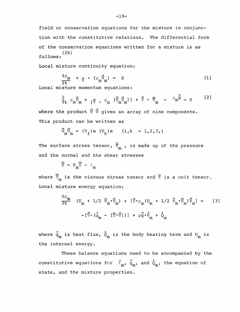
field or conservation equations for the mixture in conjunc-
tion with the constitutive relations. The differential form
of the conservation equations written for a mixture is as
(26)follows:
Local mixture continuity equation:
Pm + * (P m V ) = 0 [1]3t
Local mixture momentum equations:
+ v +vm = Om [2]7t PmVm [ m (Vm m] m
where the product V V gives an array of nine components.
This product can be written as
VmVm = (Vi)m (Vk)m (i,k = 1,2,3,)
The surface stress tensor, T , is made up of the pressure
and the normal and the shear stresses
T=P I -m m
where T is the viscous stress tensor and T is a unit tensor.m
Local mixture energy equation:
mt (U + 1/2 V V ) + [VPm (U + 1/2 V )V ] = [3]
-[V (q - [T-V])] + pg-V +m m m
where qm is heat flux, Qm is the body heating term and Um is
the internal energy.
These balance equations need to be accompanied by the
constitutive equations for Tm' qm, and Qm' the equation of
state, and the mixture properties.

-20-
2.2.1.1 Approximation to the field equations -Component Codes
Approximations which are made in solving the conserva-
tion equations in the component codes using the homogenous
equilibrium model for the two-phase flow will be discussed in
this section.
Basically, none of the existing subchannel codes use
such a generalized three dimensional set of field equations
as are given by Equations 1, 2 and 3. Rather simplifying
assumptions are made in these equations. For example, in
most of the COBRA versions, flow is assumed to have a
predominantly axial direction and all the "lateral" flow is
lumped into one lateral momentum equation. The reason for
such treatment may be justified by considering the none-
orthogonal characteristics of subchannel arrangement (Fig. 3)
which do not allow treatment of the lateral or transverse
momentum equations as rigorously as the axial momentum
equation. It is assumed that the interaction between two
adjacent subchannels in the transverse direction is through
two distinct processes,* namely, diversion cross-flow and
turbulent mixing. Axial turbulent mixing between nodes is
ignored.
The first process, diversion cross-flow is assumed to
exist due to local transverse pressure difference in the
adjacent subchannels. Such a process transfers mass, momentum
*A more general classification is given in Ref. (27) and isreferenced in the model making process of WOSUB (17). Alsosee Ref. (47) for basic notation in subchannel analysis.

-21-
Exact control volumefor transverse mom.equi
Control volume for axialmom., equation
/
Fig. 3[21] Control volume:subchannel ana
.. S... --

-22-
and energy with the assumption that the cross flow loses its
sense of direction when it enters a subchannel(4) Unlike the
HEM versions of COBRA, WOSUB which is essentially devised for
analysis of ATWS in BWRs does not account for diversion
cross flow.
The second process, turbulent mixing is assumed to be
caused by both pressure and flow fluctuation. In this process,
no net mass transfers, only energy and momentum are involved.
This is due to the assumption of the equi-mass model.* The
magnitude of the turbulent mixing term is determined either
by some correlations or by a physical model that includes
empirical constant.
All the COBRA versions account for a single phase
turbulent mixing while the two phase turbulent mixing term was
added in the versions following COBRA-II, since COBRA-I does
not account for this term.
It should be mentioned that forced flow mixing which
is caused by some rod spacing methods such as a wire wrap or
diverter vanes is taken into account, especially in those codes
which are capable of analyzing fluid flow in LMFBRs such as
COBRA-IIIC and COBRA-IV-I. Recently, a wire wrap model has
been added(2 8) to COBRA-III-P which makes it capable of
handling LMFBR flow analysis.
*The equi-volume model which is based on the change of samevolume of flow is used in the MIXER code. For further detailsee Ref. (22).
-23-
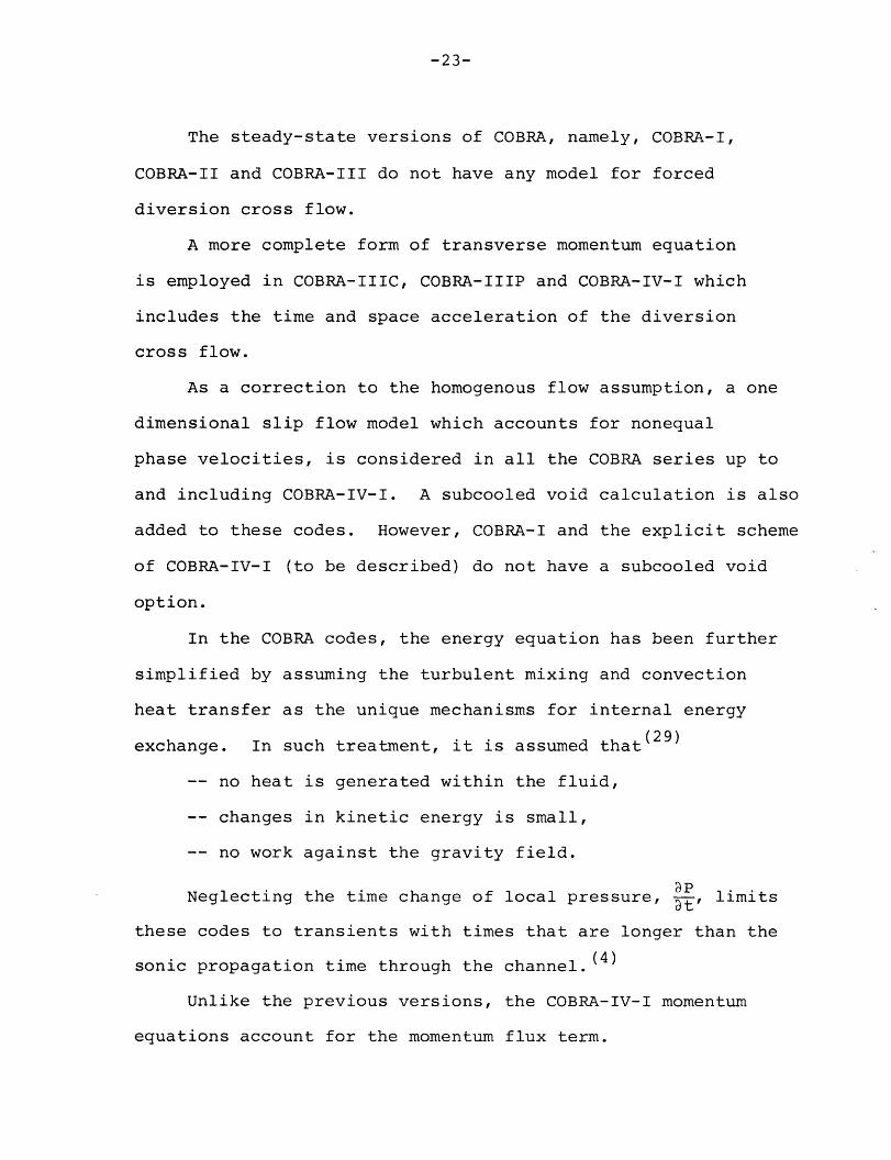
The steady-state versions of COBRA, namely, COBRA-I,
COBRA-II and COBRA-III do not have any model for forced
diversion cross flow.
A more complete form of transverse momentum equation
is employed in COBRA-IIIC, COBRA-IIIP and COBRA-IV-I which
includes the time and space acceleration of the diversion
cross flow.
As a correction to the homogenous flow assumption, a one
dimensional slip flow model which accounts for nonequal
phase velocities, is considered in all the COBRA series up to
and including COBRA-IV-I. A subcooled void calculation is also
added to these codes. However, COBRA-I and the explicit scheme
of COBRA-IV-I (to be described) do not have a subcooled void
option.
In the COBRA codes, the energy equation has been further
simplified by assuming the turbulent mixing and convection
heat transfer as the unique mechanisms for internal energy
exchange. In such treatment, it is assumed that(29 )
-- no heat is generated within the fluid,
-- changes in kinetic energy is small,
-- no work against the gravity field.
Neglecting the time change of local pressure, , limits
these codes to transients with times that are longer than the
sonic propagation time through the channel. (4)
Unlike the previous versions, the COBRA-IV-I momentum
equations account for the momentum flux term.
-24-
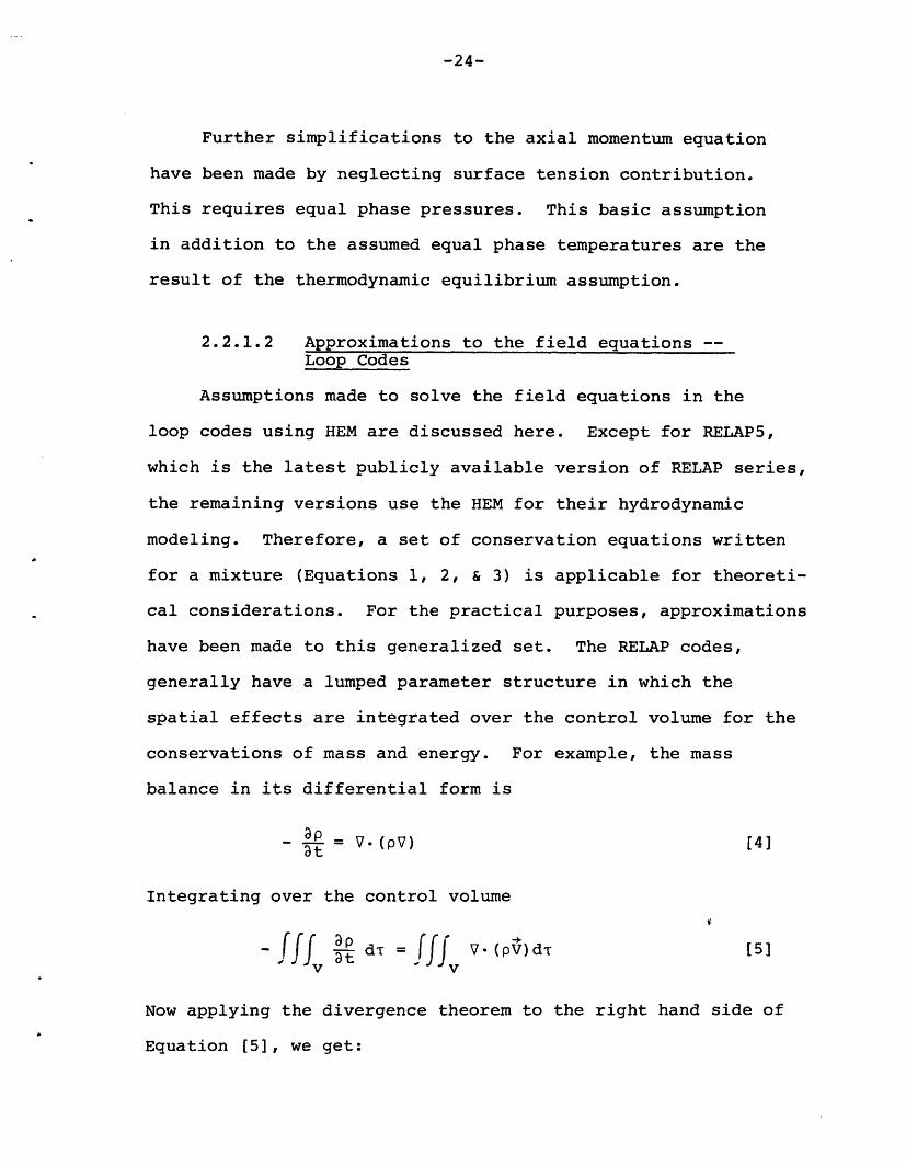
Further simplifications to the axial momentum equation
have been made by neglecting surface tension contribution.
This requires equal phase pressures. This basic assumption
in addition to the assumed equal phase temperatures are the
result of the thermodynamic equilibrium assumption.
2.2.1.2 Approximations to the field equations --Loop Codes
Assumptions made to solve the field equations in the
loop codes using HEM are discussed here. Except for RELAP5,
which is the latest publicly available version of RELAP series,
the remaining versions use the HEM for their hydrodynamic
modeling. Therefore, a set of conservation equations written
for a mixture (Equations 1, 2, & 3) is applicable for theoreti-
cal considerations. For the practical purposes, approximations
have been made to this generalized set. The RELAP codes,
generally have a lumped parameter structure in which the
spatial effects are integrated over the control volume for the
conservations of mass and energy. For example, the mass
balance in its differential form is
p = V-(p) [4]at
Integrating over the control volume
-i v at dr = fjf V- (pV)d-r [5]
Now applying the divergence theorem to the right hand side of
Equation [5], we get:

-25-
JJ -T ftV.(PV')dT= fT pV ndsV Vv v
or
n-.(pV)ds + t d = 0 [6]
s V
Using M as the existing mass in the volume J atJ
time ti and considering the term -ni .(pSV)i = W. which is
equal to the inflow from side "i" into volume J (Fig. 4),
the mass balance reduces to
[7]
dt M = E W..dt 3 i=l 13
Similarly, a simplified form of the energy equation
which has been used in RELAP2 and various MOD's of RELAP3 is
as follows:n
dt= Wij. .h. .+Q [8i=l ij1 1 j
where U. is the internal energy of volume J, hij is the enthalpy
of fluid flowing from side i into volume j and finally Qj is
the heat input to volume j.
The effect of kinetic, potential and frictional energies
are neglected in Equation [8]. However, the RELAP4 energy
equation accounts for kinetic and potential energy changes.
Unlike the mass and energy equations, the momentum equa-
tion is written for a shifted control volume as shown in Fig. 4.
This method minimizes the extrapolation of boundary conditions.
The final form of the momentum equation used in various MOD's
of RELAP3 is as follows:

-26-
j + 1A
WJ+1 = WL
pi+l
J -l-
J-1
AK
A
X
Momentumcell
Junction J
lass andenergy cell
Fig. 4 Geometry for mass, momentum and energy quations.
Flowchannelwall
a
W = WKL
---- ~I J
CJ-1 W

-27-
1 L dW.c(L d = P P + AP + Pdz kjWj j I
144gc dt i+lj 1 4 4 [9]Pj
However, like the energy equation, an improved form of the
momentum equation is implemented in RELAP4 which takes the
form: (30)
dW.I It = (P +P ) (P+P ) - F F
< -1-> z <-3- <-4--> <-5.-> < K L f>6-
L . L. L.L. I dP - I1 d(vW)
- dF - KK A [10]soK oK 1
< 7--8- > <8 > <--9 -- >
dWtIt is assumed that the junction inertia term, I dt in equa-
tion [10] or the corresponding term d in equation [9]
represents the rate of change of momentum everywhere in the
selected control volume J. (Fig. 5) In equation 10, I is
the geometric "inertia" for the flow path and also,
W. = flow rate in junction J,
Pk = Pressure in volume K,
Pkgj = gravity head contribution for volume K,
F = friction terms,
v = velocity,
A = flow area.
The significance of each term in equation [10] is as follows:
Term 1 represents the rate of change of momentum,
Term 2 and 4 represent the pressure drop between two volumes,
Terms 3 and 5 represent gravity,
Terms 7 and 8 represent the friction and pressure dropassociated with expansion and contraction.
Term 6 represents the fanning friction terms.
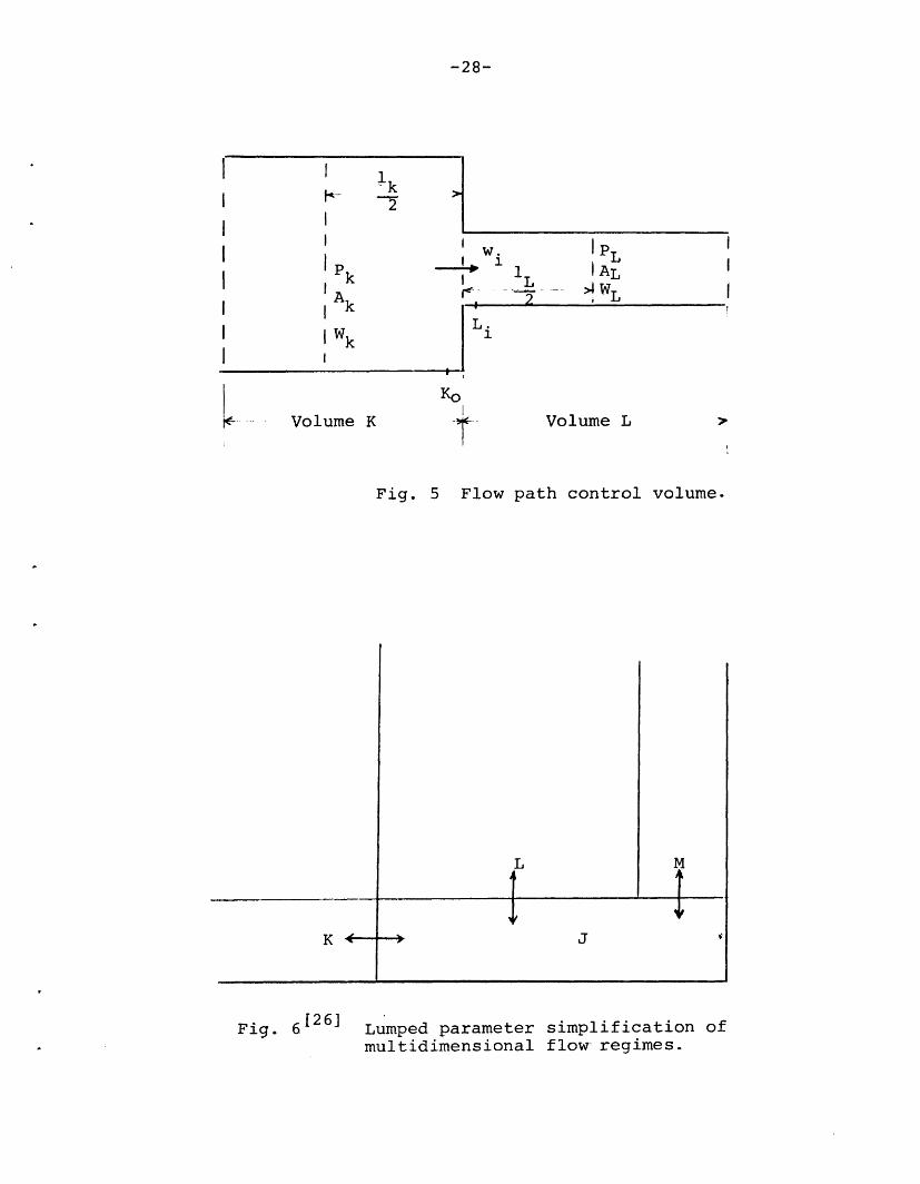
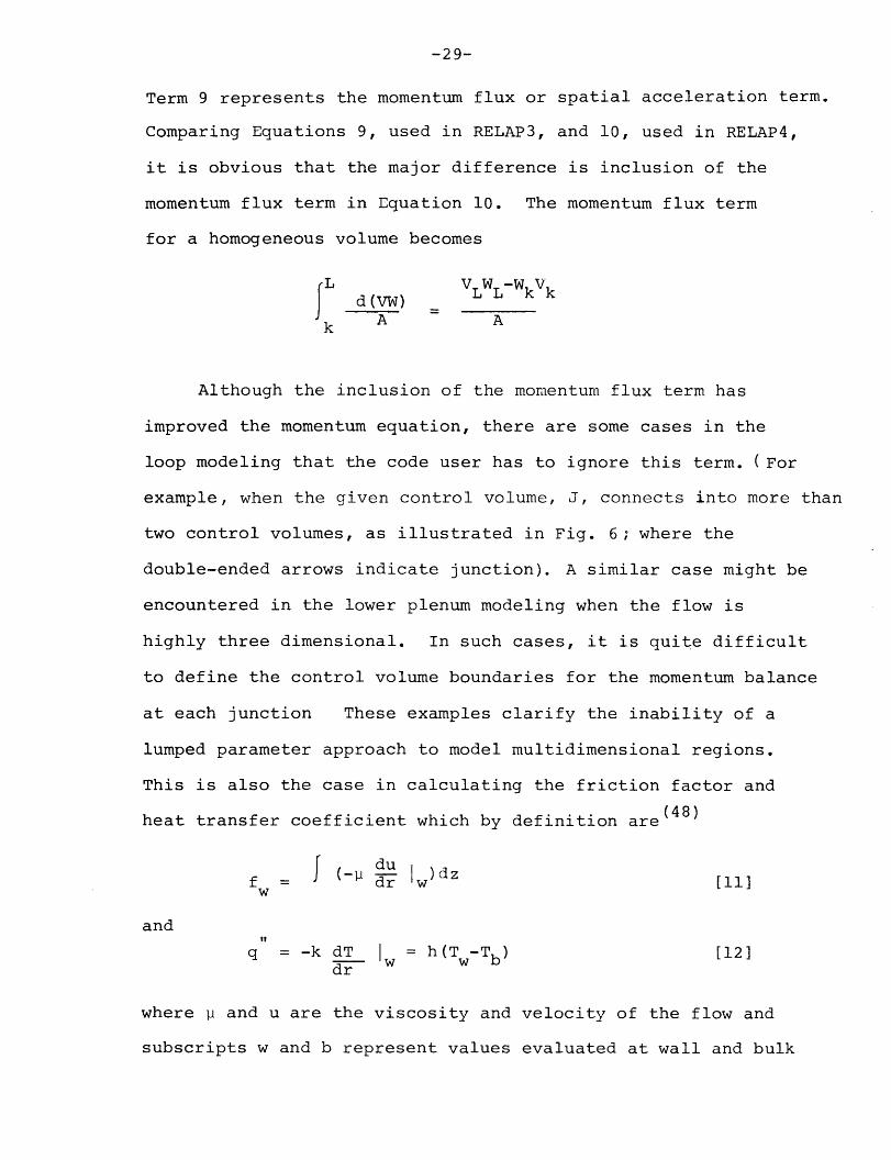
-28-
I w. IP1 ALL
r. . WL
L.1
Ko
Volume K Volume L
Fig. 5 Flow path control volume.
K -
L
t. J '
Fig. 626] Lumped parameter simplification ofmultidimensional flow- regimes.
-II
P k
IA
I k
I WkI
1k-7
!
! !-
II
i
M
t
-29-
Term 9 represents the momentum flux or spatial acceleration term.
Comparing Equations 9, used in RELAP3, and 10, used in RELAP4,
it is obvious that the major difference is inclusion of the
momentum flux term in Equation 10. The momentum flux term
for a homogeneous volume becomes
L VLWL-WkVk
d(VW) = _ _
k A A
Although the inclusion of the momentum flux term has
improved the momentum equation, there are some cases in the
loop modeling that the code user has to ignore this term. (For
example, when the given control volume, J, connects into more than
two control volumes, as illustrated in Fig. 6; where the
double-ended arrows indicate junction). A similar case might be
encountered in the lower plenum modeling when the flow is
highly three dimensional. In such cases, it is quite difficult
to define the control volume boundaries for the momentum balance
at each junction These examples clarify the inability of a
lumped parameter approach to model multidimensional regions.
This is also the case in calculating the friction factor and
heat transfer coefficient which by definition are(4 8 )
du )dzf = dr w) [11]
and
q =-k dT w =h(Tw-Tb) [12]dr w
where and u are the viscosity and velocity of the flow and
subscripts w and b represent values evaluated at wall and bulk

-30-
respectively,
It is clear from equations 11 and 12 that the deriva-
tives are evaluated at the channel wall. However, since a
lumped parameter approach doesn't account for velocity and
temperature profile, therefore, the above mentioned derivatives
do not make sense. It is this reason which necessitates an
input specified friction fractor for the codes using this
approach.
The junction inertia term is another term in the
momentum equation (Equations 9 and 10) which becomes rather
ambiguous in modeling the complex geometries. The junction
inertia arises from an approximation in the momentum equation
to the temporal inertia term as follows:(30)
x2 1 dw dx _ dw 2 dx___ dx dx 1I [13]J AX x)T dt l A(x) dw ( I dt
where x = center of control volume 1 and x2 = center of
control volume 2, and I is the geometric inertia for the
flow path defined as:
I -(2 dx [14]1
The geometric inertia for a homogeneous volume, Fig. 4,
a bbecomes I = 2A + 2A , however for complex geome,trics,
K L
the inertia term may be determined by using a simplified
assumption. The basic assumption which is introduced in this

-31-
(30)respect is that the inertia of a junction is composed of
two independent contributions, one from each connecting
volume. For example, Fig. 7 could represent a downcomer
region. If we assume that Junction 1 communicates primarily
with Junction 3, then with respect to the mentioned basic
assumption, the geometric inertia will be:
Ij = Ijl + Ij2 + Ij3 [15]
or
L1 L2 L 1I - + 2 + 1j =2A1 A2 3
Where L 1 is the effective length of both Junctions 1 and 3 and
the effective length of junction 2 is assumed to be 2L2.
f' '-
0L1
I , - - :
I II L 2
I1A I
= Junction number
O --- = Flow Path
Fig. 7(30) - A Downcomer Representation in RELAP4
A schematic of RELAP4 model of a PWR is presented in
Fig. 8. It illustrates the complexity of accounting for all
volumes and junctions in a LWR plant.
\
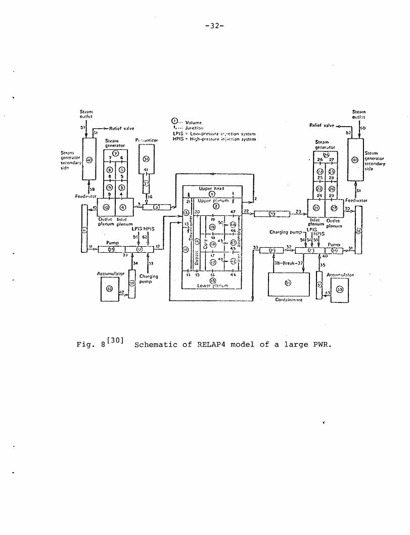
-32-
Steamrs sexis
Stwnimgensrasecondside
Fig. 8[30] Schematic of RELAP4 model of a large PWR.
Stearn
0leammenerator.condaryde

-33-
2.2.2 Improvements on the Homogeneous Equilibrium Model
By retaining more field equations, a more realistic
approach to analysis of severe transients has become possible
in reenct codes. The increased number of field equations enable
a code to analyse transients in which the situation is far
beyond the capability of the rigid assumption of equal phase
velocities and temperatures. In this respect, countercurrent
two-phase flow and vapor-liquid phase separation during
small break transients and emergency core coolant delivery
are notable examples.
Since in a non-homogenous flow slip exists between
the two phases, there is a relative motion of one phase
with respect to the other. This relative motion arises
due to density and/or viscosity differences between phases
where usually the less dense phase will flow at a higher
local velocity than the more dense phase, except for the
gravity dominated flow(1 8 ) The general effect of slip is to
lower the void fraction below the homogeneous value.V
The slip or hold up ratio, s = g should not beVL
confused with the slip velocity VsL = VL - Vg, or drift
velocity, a concept which is used in the drift flux model.
Unlike the one-dimensional HEM, a non-homogeneous,
one dimensional flow calculation for a two-phase flow in
thermodynamic equilibrium, involves the solution of one

-34-
equation of state and five differential equations: a
mixture energy equation and one continuity and one momentum
equations for each phase as it is done in RELAP5.
2.2.2.1 Dynamic Slip Model
Simplified assumptions have been made to reduce the
number of conservation equations while retaining the
improvements over HEM codes. This is done in WOSUB and
COBRA-DF by using the concept of diffusion or drift flux
model, and in RETRAN by introducing the dynamic slip
model.
RETRAN computer code is basically developed from the
RELAP series of codes. It is a one-dimensional code which
solves four field equations written for a fluid volume
as follows: Mixture continuity, Momentum, Energy equation,
and time dependent behaviour of the velocity difference,
obtained by subtracting the momentum equations written
for each phase. This additional momentum equation reads:
SD (1 1 P 1 1g DX DX P9 g X a Pk cc9P
AgL BgL sL ° [16]
where V,p,a,P represent velocity, density, void fraction and
pressure respectively. Also Ag L represents the surface area
between vapor and liquid phase per unit volume and BgL
represents the friction coefficient between vapor and liquid

-35-
phases.
In deriving equation (16), the following assumptions
have been made:
1) The wall friction is nearly equal for the two-
phase.
2) The momentum exchange between phases due to
mass exchange is small.
In addition to inclusion equation (16) in RETRAN,
some improvements have been made in the field equations
used in RELAP4, as follows:
1) Additional term in the mixture momentum
equation with respect to the momentum flux. Mixture
momentum flux:
ax [A (agPg (V2)g) + al (V2 )1] =
a +a VsL l 9Plg A
Additional Term
2) Additional term in energy equation which accounts
for the time rate of change of kinetic energy,
at [ U2[pA(-)].at 2

-36-
3) Using a flow regime dependent two-phase flow friction
multiplier.
2.2.2.2 Drift Flux Model
Unlike RETRAN, COBRA-DF which is a vessel code and uses
the drift flux model, employs five field equations to determine
phase enthalpy, density and velocity*. This code is used
exclusively for examination of upper heat injection of water
during a LOCA in a PWR.
Vapor diffusion or drift flux model is another step
toward modeling a non-homogeneous non-equilibrium flow. The
basic concept in this model is to consider the mixture of the
two-phase as a whole, rather than treating each phase separately.
The DFM is more appropriate for the mixture where dynamics
of two components are closely coupled, however, it is still
adequate where the relatively large axial dimension of the
systems gives sufficient interaction time (26)
In this model in addition to the three field equations
written for the mixture, there is a diffusion
* THOR which is developed at BNL (31) uses the DFM and accountsfor thermal non-equilibrium of the dispersed phase only.

-37-
equation written for the dispersed phase which reads:
ap O -t -+ [17]gt + V(agpg Vm) = r - V (gpg Vgj) [17
where r is the phase change mass generation, Vgj and Vm areg gm
the drift velocity and mixture velocity respectively.
WOSUB which is a BWR rod bundle computer code uses the
DFM and solves four field equations written for a subchannel
control volume, as follows:
1) continuity equation for mixture
2) continuity equation for vapor. This equation reads:
at (Pg9ai)i+A (P gJg) i = Ap gii + Pgi qgi [18]
where J = vapor fluxg
qgi = vapor volume flow to subchannel i
T. = vapor volume generation in subchannel iper unit volume
Equation 18] indicates the fact that the temporal and
spatial increase in the mass of vapor in subchannel
i is due to vapor generation in the subchannel and
vapor addition from the adjacent subchannels. The
vapor volume generation term, , appears in Equation
[16] due to using the DFM. This term is part of the
code constitutive package. It is modeled in
WOSUB based on the Bowring's equation which relates

-38-
Y to the heat flux:
i-TAp h q [19]v fg
where T is a coefficient depending upon coolant
condition, Ph is the heated perimeter and q" is
heat flux in the fully developed nucleate boiling
region, and A is the flow area. 'The effect of
subcooled boiling non-equilibrium condition is
considered in the final form of .
3) Mixture axial momentum equation: This is
the only momentum equation considered in the code.
Therefore it is clear that WOSUB is strictly one
dimensional. This may be justified by considering
the fact that the intention of creating WOSUB,
has been analysing the flow characteristics in
encapsuled PWR bundles as well as BWR bundle
geometry 17) in which, based on a channelwise
node, the flow is predominately one dimensional.
Nevertheless, the transverse effects are not
totally forgotten. In fact a natural turbulence
exchange mechanism is considered. Furthermore,
vapor diffusion accounts for the tendency of
diffusion vapor in the higher velocity regions.
-39-
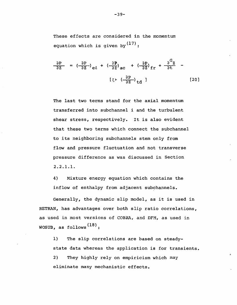
These effects are considered in the momentum
equation which is given by (1 7):
ap ~ P aGz9LP (-I)P) + +Paz az )e+ az)ac + t)fr at
[h ( az )t d [20]
The last two terms stand for the axial momentum
transferred into subchannel i and the turbulent
shear stress, respectively. It is also evident
that these two terms which connect the subchannel
to its neighboring subchannels stem only from
flow and pressure fluctuation and not transverse
pressure difference as was discussed in Section
2.2.1.1.
4) Mixture energy equation which contains the
inflow of enthalpy from adjacent subchannels.
Generally, the dynamic slip model, as it is used in
RETRAN, has advantages over both slip ratio correlations,
as used in most versions of COBRA, and DFMI, as used in
WOSUB, as follows (18 )
1) The slip correlations are based on steady-
state data whereas the application is for transients.
2) They highly rely on empiricism which may
eliminate many mechanistic effects.

-40-
3) The slip velocity VsL = V - VL can only
assume positive values, hence the possibility
of rising liquid and falling vapor cannot be
predicted.
2.2.3 The Two-Fluid Model
The inability of the simplified methods to treat the
multidimensional, non-equilibrium separated and dispersed
flows necessitates a better modeling of the two-phase
flow. Anticipated reactor transients and postulated
accidents like LOCA specially require a more realistic
treatment.
Those cases in which a one-dimensional HEM is not
acceptable are tabulated in Table 2-1.
TABLE 2-1(32)
CASES WHERE 1-D HEM IS NOT
ACCEPTABLE
MultidimensionalEffects
Downcomer region
Break flow entrance
Plena
Steam separators
Steam generators
Reactor core
Non-EquilibriumEffects
ECC injection
Subcooled boiling
Post-CHF transfer
ECC heat transfer
Low-quality blowdown
Reflood quench front
PhaseSeparation
Small breaks
Steam generator
Horizontal pipe flow
Counter current flow
PWR ECC bypass
BWR CCFL
-41-
The most flexible approach in modeling these cases
is through using a two-fluid, full non-equilibrium concept,
which is the most sophisticated model employed so far in
treating the two-phase flow.
The derivation of the field equations in their general
tensor form is quite involved. A detailed derivation is
presented in Ref. 33. A short-hand representation for the
two-fluid model is 2V2T or UVUT which stands for unequal
phase velocities and temperatures - whereas lVlT or EVET
is used for HEM.
The unknowns and equations in this model are
summarized in Table 2-2.

-42-
Table 2-2
Two Phase and Single Phase Comparison
with Respect to the Flow
Equations
Case Unknowns # of Unkn. Type of Euations # of Egu.
Single V 3 Conservation of Mass 1
Phase P 1 " of Momentum 3
Flow T 1 " of Energy 1
p 1 Equation of State 1
6 6
a(void fra.) 1 Liquid Balance Equ. 1
V 3 Vapor " "g
Two* V 1 3 Liquid Mom. " 3
Phase P1 1 Vapor " " 3
Flow Pg 1 Liquid Energy 1
P 1 Vapor " " 1
T 1 1 Equation of State 2
T 1 in Each Phaseg
12 12
* Table 2-3 gives a more detailed description of variousapproaches to modeling the two phase flow.
-43-
The two-fluid concept is employed in the advanced thermal
hydraulic codes such as COBRA-TF, from BNWL, TRAC, KACHINA*,
SOLA-FLX, SOLA-DF from LASL and finally THERMIT, which is
developed at MIT under EPRI sponsorship.
TRAC is the state-of-the art primary loop analysis code.
It employs a three-dimensional 2V2T model for the vessel and
a one-dimensional drift flux model for the rest of the primary
loop. The reactivity feedback is accounted for through coupling
the point kinetic equations to the thermal hydraulic model.
The same concept of volume and junction defined for RELAP
series is used in TRAC as well. A cylindrical coordinate
system is used in TRAC for modeling the three-dimensional
reactor vessel. This doesn't satisfy the purpose of a common
reactor core analysis with its square array pattern governed
by the bundle design. THERMIT which is a vessel code, is
basically the cartesian version of TRAC. Hence, the same
field and constitutive equations used in TRAC is employed in
THERMIT as well. A core or a fuel pin analysis in THERMIT
essentially is based on treating a whole bundle cross-section
as one node where the local details have been smeared throughout
the cross-section. Therefore, neither TRAC nor THERMIT account
for a turbulent mixing process. Devising a subchannelwise
version for THERMIT using a coolant centered control volume
* K-FIX and K-TIF are two versions of KACHINA developed atLASL. The first stands for fully Implicit Exchange numericsand the second for Two Incompressible Fields.

-44-
has been initiated at MIT. This version will include
a turbulent mixing model.
A summary of the aforementioned two-phase flow models
is present in Table II-3. The notations and a description
for specifications used in this Table are as follows:
a) A partial non-equilibrium model, Tk Tsat,
assumes one phase is at saturation, temperature
of the other (k) phase computed.
b) The notations T,q,r,M and E stand for viscous
stress, conduction heat transfer, interphase
mass, momentum and energy exchange respectively.
c) The notations: Vr, VG - V, VG - J stand for
relative velocity, diffusional velocity and the
drift term respectively.
A glance at this table shows clearly that although
the 2V2T model imposes no restriction on the flow condition
such as velocity or enthalpy, however it contains the
largest number of constitutive equations and it seems that
the empiricism which enters in these equations is introduced
at a more basic level than the less complicated models such
as 1V1T approach.

-45-
IH W It
r-
mCN,_-
mI
Q)Hl
Ero
ro0
U)
a
0
0
Qlr-
a)0
w~

-46-
I(N
-I
rdE-
or0
.HQ-
0'
U)0I
o
1b
d
0o

-47-
2.3 Classification According to Range of Application
2.3.1 LOCA CODES
The major task of thermal-hydraulic LOCA codes is
analysis of the severe cases that are encountered by the
reactor core or the primary loop during the period of a loss
of coolant accident. The four phases of a LOCA, for a PWR
double ended cold leg break, in order of occurrence are as
follows:
1)*- A blowdown phase which generally lasts for 30 seconds,
with 2200 psia initial pressure, and ends when ECCS starts
to work.
2)- About sixty seconds after break initiation ECC fills the
lower plenum and reaches the bottom of the core (Refill Phase).
3)- The refill phase is followed by a REFLOOD phase which lasts
for about 150 seconds, during which the core is fully flooded
and quenched by the coolant.
4)- Long-term cooling then follows.
It has become customary to call a code a LOCA code even
if it is capable of describing only the first phase of the
four aforementioned phases. At the same time two codes that
are capable of handling the blowdown, may be entirely
different with respect to their type. For example, one can be
a component code whereas the other a loop code. To avoid any
* This step is divided in two periods according to Ref. 31,namely: a) Adiabatic Liquid Depressurization, b) The BlowdownPeriod.

-48-
confusion, a classification is necessary with respect to
the code's application and type, in addition to the
physical models and numerical methods. A usual way to
classify the LOCA codes is by categorizing them into
two groups as follows.
2.3.1.1 Evaluation Model Codes
The first group contains those codes which employ a
conservative basis for their physical models. Such
conservatism is mandated to satisfy the NRC acceptance
criteria. These codes are called the EM-codes for Evaluation
Model. They constitute the WREM package which has the capa-
bility to analyse the postulated LOCA with ECC injection in
(35)accordance with current commission acceptance criteria
The codes which constitute the WREM package (36) are the
existing computer programs which have been modified to comply
with the USNRC criteria. Most of the RELAP series of computer
codes are a LOCA Licensing code such as RELAP4-MOD5 and
RELAP5-MOD7. Whereas RELAP3B-MOD101 is essentially devised
to analyse ATWS and RELAP4-MOD6 and RELAP5 are not based
on conservative correlations. RELAP4-EM is the only version
of RELAP which is specifically modified to comply with
acceptance criteria.
The present EM codes comprise an assembly of codes
run sequentially. Each member of the sequence is a stand-
-49-
alone code developed for some special application. With
this respect, RELAP4-EM in conjunction with RELAP4-FLOOD (3 6)
and TOODEE2 (37 ) constitute the WREM package which perform
the PWR LOCA analysis. Also a combination of RELAP4-EM
and MOXY-EM (3 8 ) constitute the WREM package for a BWR LOCA
analysis. The respected procedure for the above mentioned
analysis are presented in Fig. 8 and 9.
2.3.1.2 Best Estimate Codes
Most of the LOCA codes lay in this category. The
basic physical models used in these codes ely on the best
estimate assessment rather than conservative correlations.
Unlike the EM-codes, the BE-codes are mostly devised as
one large system code consisting of various functions
previously performed via the separated stand-alone codes.
This guarantees the proper compatibility and continuity
between the various calculational phases. As an example,
the multi-purpose loop code TRAC can be used for the analysis
of the whole phases of a LOCA namely, blowdown, refill
and reflood. Unlike the EM-codes which mostly use a homo-
geneous equilibrium model in conjunction with a lumped
parameter approach for their analysis, the best-estimate
codes are much more demanding and the most recent BE-codes
employ the state-of-the-art physical models. Therefore they

Uw Z
0 DUC~
E-40
E
O D=r Ep
Qz
0,<4
I
U] E4U E- f
.1
h r=
E- U O UE- U 0
pOPP4
U) Lncn r- H
.,
0E-
H 4 Er
D E4
U
-50-
Q00
w1Y
¢00IIr
II
5I
F:14
wP4
OO
0E-
o0H
I
p:
1-4
Hh
N.,
CNJ 0CN C 12
z :Rpq 0ccn
i-1z
0
0-::PQ
W
E-1
UH H
Z
W
H
I 6
jI'N
r
J
t
ol-
- |

0zH
HOQ
O z
0H
O HeqV 14
PI
Eq
0U
o
Hz z
O r
EHH
0 <
! P4U C:
H U)A Z *HqU H U
0 d
p o0
ml
,t
Ln
o
-51-
Z0H
P4
0
U
U_D
W
P20
HE-4H
0W>-
5
P
3P4
Cl)WHU]
W5:W ZE-4 F:
H UEH~D ]~H
K a
$4 zz ::
i I i

-52-
can be used to evaluate the degree of conservatism employed
in the licensing (EM) calculations.
No codes have specifically been devised to handle the ATWS
type of transients. In Table II-4 the causes and consequences
of ATWS transients in both PWR's and BWR's are shown.
3. Two-Phase Heat Transfer Model
The energy balance of the field equations contains
the contribution of the so-called wall heat transfer which
accounts for the amount of heat transferred into or
out of the control volume through a combination of convection
and conduction heat transfer. This requires models for the
wall heat transfer.
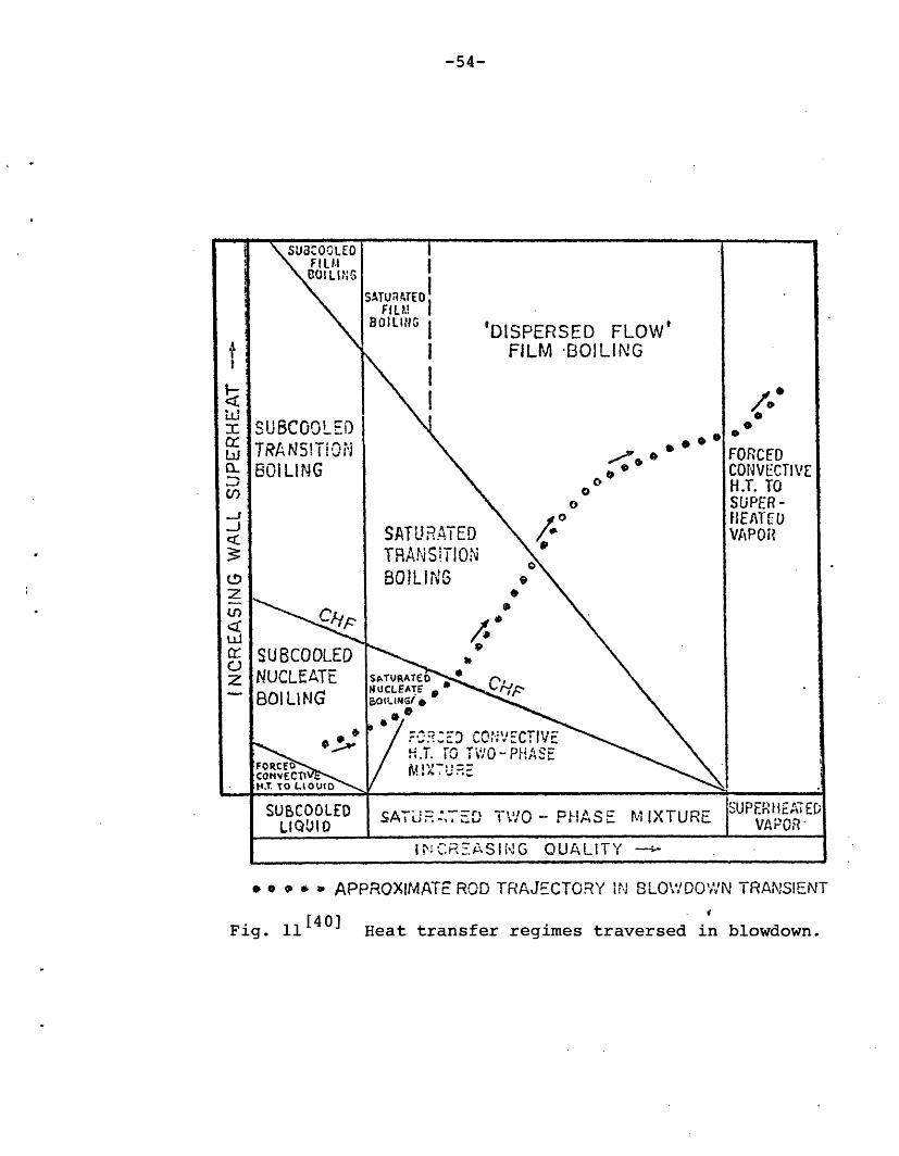
During hypothetical LOCA's, nearly all the two-phase
heat transfer regimes are experienced by the coolant in
the core of the NSSS, the steam generators, and the pipe
of the hydraulic loop (see Fig. 11). This interdependence of
the hydrodynamics and the wall heat transfer, as shown in
Fig. 12, is accounted for in the thermal hydraulic LOCA
codes through using a two-phase heat transfer package.
These regimes are elaborated on in a pool boiling curve
drawn for a fixed pressure, and shown in Fig. 13. According
to Fig. 13, the path ABCDEF is obtained in a temperature

-53-
ot
- O P k to 0)
0) O a) -H)4-0 O a) -rq
f 0 c *H 0) UH UH k 4 m U)
4 04-Hr-H
4Prda)
>(D
N
-*H 0 --H
0 U0)
) 4
IN
,--I ,-- i a) a ·,E ,:1 "4:3 ):) ·- *H . i,H r4 " 4 4 r : rd IN ·d d ( -O - ,H 4 U)-H-H r .O) O . q i 0 I H)
r, . /L
In l.. .- . I * :O - ,-I
OO 0 I
O . O ~ O-. k
mu aoU) E$ r -)o O O (D O · O O,' OOU Oa ) U )
4 43 4 H
I -:>to t 44 04J
43 t )0 ) ) *H 04O nl ., - I > 0::J > I
) O > -d - U IH-H4J k k) a) 4 10-P- O
". O 4 ¢ O-k -H C 3Z O Z UH O a O 0 r Q H U H .# . , H > k En
t m4. 4--H ) a
HH <. 3 k si
P m4 k 3 P* O O O k
H) O 00r ·4
U)0)
0l)t70-
01)U)
0u
> -i �4 U) 0 U54 $ I H 04
M U) Q) QH*i 0) U H
54 4 rQ 0P 04-H -
OO
O 'a O U
En a) ro cJm r. o,- r4 CV
U)
O >)0 >
I 1)
-1 (D (0(00) a)E! 040) 5-4*H ~ 5-1 C)5-4 0 :: 0)a 4. 4.3 "O
OH( 0) 0
0) a)
0 0U 5-
O U4 U r 4
r-i I ·i 0 044 .- -- 4
a) 5-4
·H 0 4) --HO 4-3O)
,-4 I 0),-4 ol 3 q) -EC0) to F. 04- Id3 d H f (a 0)O 0 k c)-H kP4 H 4P 4 kU
1Ia)
Or8 3-I a
0-HI 0rIO',-I-Pu O
0
O
0 -,
Id ~U)0) IPO O- g UoH E a040HH, 04H 1'4 - -4 H0 4J4J L R
i- ,--
Imd
O ,O OO rCCf
U)
U)(a
3UO OPm"O
E4
r u- (a
(D I
-I O - 0 EI
4 ( Q) -H4k k Wl k 4 3.-)P4 5 UI k
. O
w 3u 0> I n
t0 k 1 a D04 44 P U) tr 2
k i
c))* . -) --I I> k > > mUU
.,q 0 r *H -H 5.-ri d >i4 .U) ) I 0 w .0)4itId C 4u -H U (d a4w k 4-H
)O H4) O O ) 0IW4-Z 0404-U Ok Z U 0c4
) 4- -H 0)E U4 5r - U)
4 rId k Id k 3 )O aH - O Q)k
u) ) UO a0'~~~ _
404rd
0)
Od O 1
>1-i,-
.-40 -H0 ri
En to En)-H0()w 0 m X a:
~-14-4 i-l (d 104
L 3 1fuz t *1 u),B
I 0)
-H k 4
4 4J 4J -H
0I
-H
I I t
.H to 4
0)00O k- -H -P
4.
0 ri:3O
04 O 3>0
: -iH H-04-I 4
U;
to
(0
En
ICN0)1(l
(dE-4
Itzr ,Ln 0"-
. . _
.- ----- -- -C . _---.
__
-54-
SUBCOOLEDTRA N5! i O11 , 'BO1LING
SUBCOOLEDNUCLEATEBO Li NG
FORFCCONVECtiLH.T. TO LlOUtD
SUBCOOLEDLIQUID
'DISPERSED FLOW'FILM BOILING
S S
'* -/0 oFORCED'~ · ~ CONVECTIVE
oo H.T. roo SUPER-
0\ Io SlEAlTE SAT . RAT ED / VAPOtTRAN S! T! ONBO LING
A ·SAT! ED
CLEATE 0
r.TS i.'O-,t? \'
/~tx7~~C
__$ATU A .O .fAS '-TR SUPEH EA ES, .L. D 7 -'l , .- Pt' I IXTURE VUPEOR' Iq...............
i r- CR.ASI,G QUALITTY -
Fig. 11 Heat transfer regimes traversed in blowdown.
ii
i
ii
'2;
W.
04
Cl)
CL-0
2L)crC,
zt3l7-kn
* * e a . APPROXIMATE ROD TRAJECTORY I,, SLO\'¥.DO'w'N TRANSIENT
I -
II i _
- ___ ��-- _--�_,__I __I
.

-55-
I( -,; I?.g ir-,.:, ;..II ... . ...... .__
f ;i l I e - P. s E
L. i qidDeficient
?ist, Sprcty orDisper s ed
Annular orFilm
Slug ,Ch::rr,or Froth
B3ubbl tFroth
Sinjl..-P\',atr
L-
C
'I,
.
I'
·- ., I
k23cc). .D
0' '.I I,
P 9)
P,,
'0
.
* I .,I 9
I
AFI'.
.Oiivetcti ll toupt:rhoJ 'icj St:.-rn
¢oivection endfRadiation toSoturoted Liquid
Critical t4sut Flux4( dryout)
IForced ConvectionThroulh li.lultd Flm
.1
I[
Suhcooled l-Jiling
(:nnve clion to.'ater
Fig. 12 [19]
toS I tein
ond
nvoct;ontio.n
por Firn
I uot Flux
n oii.)
n to
Floa
Flow and heat transfer regimesin rod array with vertical upflow.
TreritJ f-r~ I':;I'L1lle-jo Tron!.', !r
r
=·
r··:
�··-··-
-,rr·
-· -35i`.2·r·.
·�5`
· ·
-.r.I-:i
·- ·
,�'r
r·t··
r. ·
f�
:·.
·:
'."
··
r
�-
I
I
f
I
INuc!!;te 3ih
I
r
._
P 0 Ji
-

-56-
t-
TVCOa
j
ItCC
(SH Z,I./nljE) ,,b 'Xnl .V3H 33Vians
I-,.
C',
I- n to,
- (ACa
0F. E a).Ein asI-- w Q eC to,
ar X
X XIL
Eo
._1
LL
lf

-57-
controlled surface as the temperature is increased. In
general, the same path on cooldown process is not followed
in the heat-up process by the boiling mechanics. For
example in a heat flux controlled surface, the path
ABCC'F will be followed in which point c' indicates the
new equilibrium state of the surface at the heat flux
value qCHF
At steady-state operation conditions, a NSSS fuel
rod is a heat flux-controlled surface with a non-uniform
axial heat flux distribution. In this case a reduction
of the heat flux may be traced on the curve of Fig. 13
by the path EC'D E'BA(1 8 ).
Unlike the steady-state conditions, during a hypothe-
tical LOCA it is not lear which mechanism prevails, since
the fuel rods of NSSS's may behave as heat flux-controlled
surfaces for some parts of the transient and as temperature
controlled surfaces for other parts of the transient.
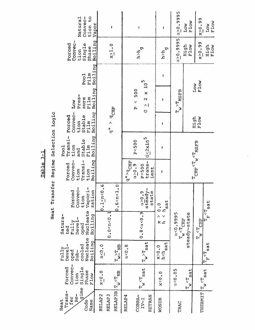
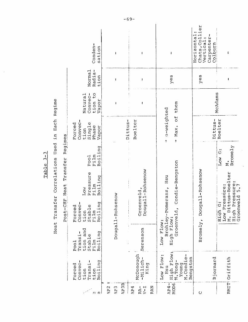
3.1 Heat Transfer Regimes and Correlations
The recent thermal hydraulic LOCA codes have increased
their capability of the two-phase heat transfer assessment
by inclusion of more distinct heat transfer regimes and
using more realistic correlations for calculations of the
heat transfer coefficient in each regime.

-58-
As was discussed in section 3.1, a stand-alone LOCA
code is capable of handling only one phase of hypothetical
LOCA's, whereas integrated LOCA codes such as RELAP4-MOD7
and TRAC have the capability of calculating both blowdown
and refill/reflood phases of a LOCA. This capability
is made possible through inclusion of the unique features
of bottom flooding (in PWR) and top spray (in BWR) of
reflood heat transfer, in the blowdown heat transfer
package. Such features are quench front, rewetting and
liquid entrainment. Also thermal radiation and dispersed
flow film boiling are specially pronounced in reflood heat
transfer and are treated explicitly in the reflood heat
transfer packages*.
The heat transfer package which was used in the early
versions of the RELAP series such as RELAP2, is used
extensively in the thermal hydraulic codes**. This package
is used in various versions of RELAP3 as well as RELAP3B-
MOD101. Later it was modified by replacing the quality by
void fraction to determine the pre-CHF heat transfer
regimes and by treating the transition boiling explicitly
in which case the heat transfer coefficient is calculated
using the MC DOUNOUCH, MILICH and KING correlation. Also
* See REFLUX (39 ) package which is developed at MIT toanalyse the reflood phase of a LOCA.
**This package is essentially adopted from the THETA hot-channel code.
-59-
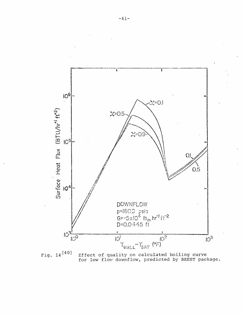
the Berenson and Groeneveld correlations were added to
the formerly existing Dougall-Rohsenow correlation in the
film boiling regime. RELAP4-MOD5 and RETRAN use this
modified version and a simplified form of this new
version was implemented in COBRA-IV-I. RELAP4-EM employs
the new version with further modifications to satisfy
the acceptance criteria. For example return to nucleate
boiling is precluded once CHF happens. Also the GE
correlation is added to the CHF correlations as an
option to replace the Barnett correlation for BWR analysis.
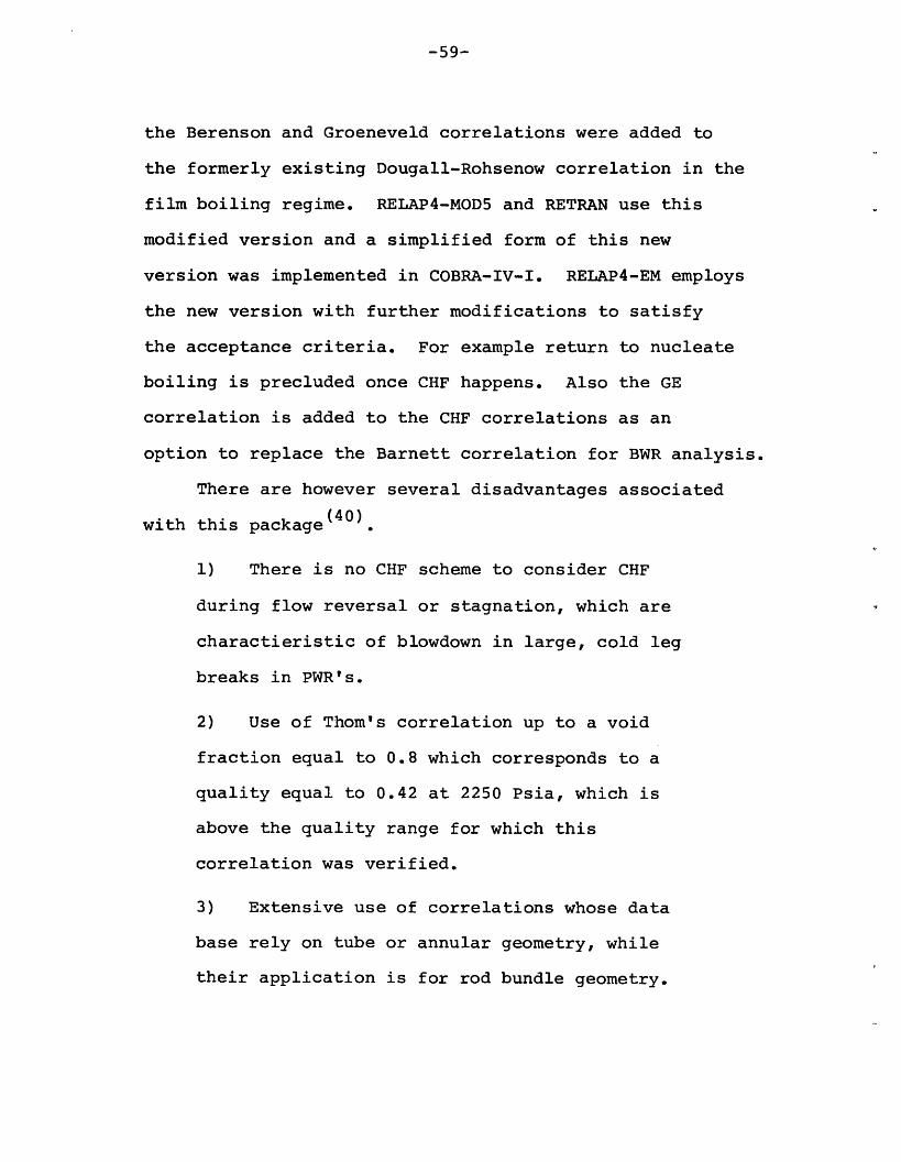
There are however several disadvantages associated
with this package(4 0 ).
1) There is no CHF scheme to consider CHF
during flow reversal or stagnation, which are
charactieristic of blowdown in large, cold leg
breaks in PWR's.
2) Use of Thom's correlation up to a void
fraction equal to 0.8 which corresponds to a
quality equal to 0.42 at 2250 Psia, which is
above the quality range for which this
correlation was verified.
3) Extensive use of correlations whose data
base rely on tube or annular geometry, while
their application is for rod bundle geometry.

-60-
4) Using the correlations which have a steady-
state data base for transient conditions.
For this reason a heat transfer package called BEEST
developed at MIT to overcome these drawbacks. BEEST (40 )
stands for BEst ESTimate heat transfer analysis. It is
based on best estimate assessment rather than conservative
correlations. Several tests of BEEST showed that it is
able to construct the complete boiling curve where
different heat transfer regimes are smoothly connected
(Fig. 14). The heat gransfer selection logic in this
package is based on the comparison of the clad surface
temperature with the two distinct temperatures on the
boiling curve, namely the temperature at the minimum
stable film boiling point, TMSFB, and the temperature at
the critical heat flux point, TCHF (Fig. 13). This is
certainly an unambiguous, efficient and valid criterion for
selecting the appropriate heat transfer regime. Once the
regime is identified, the second step is to apply a chosen
correlation for the heat transfer regime selected. The upflow
and downflow heat transfer are treated separately through
using the void fraction. The transition boiling in this
package is treated in a unique way. This treatment is based
upon an interpolation between the Q"MSFB and Q" CHF (which
are the heat flux corresponding to the TMSFB and TCHF) with
-61-
+4.4-
-
I-
LL
CO
de
i1v iC)' IC0' 1TwA - ~,,~. (°~)40] Effect of qua lty on calculated boiling curve
Fig. 14 [40] Effect of quality on calculated boiling curvefor low flow downflow, predicted by BEEST package.

-62-
respect to the temperature ratio as follows*:
Q" = E Q"cF+ (l-E) QM [21]TB CHF MSFB
where
E = (Twall TMSFB)/(TCHF TMSFB)
In equation (22), E may be interpreted as the fraction
of wall area that is wet. BEEST uses the Biasi correlation
for the CHF calculations. The Biasi correlation is
essentially a dry-out correlation. Therefore it is
appropriate for high flows and qualities where the vapor
is a dominant factor leading to dry-out. For low flows
and qualities the void-CHF correlation developed at MIT
is used. The RELAP heat transfer package which was
discussed earlier uses the Barnett correlation as well as
* This concept was first introduced by W. Kirchner(see Ref. 41), in the form of a Log-Log interpolation:
CHFTwallTB ( T ) where
wall sat CHF
Log Q"C - Log QMSFB
Log TCHF - Log TMSFB
Kirchner then applied his model in the heat transferpackage of TRAC.

-63-
the modified Barnett and the B&W-2 correlations for
the CHF calculations. In the pre-CHF regimes, the Chen
correlation is used in the subcooled nucleate boiling,
saturated nucleate boiling as well as forced convection
vaporization. This correlation has predicted the
existing data with reasonable agreement (3 8 ) as compared
to the other correlations such as: Dengler-Addams,
Schrock-Grossman, Bennett et al, Sani and finally
Guerrieri - Talty. The Chen correlation is applicable
to flow regimes from slug flow through annular flow.
While its data base is for low pressures (4 2 ) , in most
applications it is used at elevated pressures. Also,
its dependence on the wall temperature which necessitates
an alternative procedures, makes it less desirable.
The advantages of the BEEST heat transfer package
namely, treating the upflow and downflow separately, using
a once through heat transfer regime selection logic, using
wall temperature as a heat transfer regime selection tool,
using a best estimate assessment and incorporating the new
improvements in heat transfer, has made it acceptable to
the state-of-the-art LOCA codes. THERMIT uses BEEST with
some modifications such as replacement of the void fraction
calculated from DFM by that calculated in THERMIT. TRAC
heat transfer packages is also very similar to BEEST. In
fact it can be considered as an improved version of BEEST
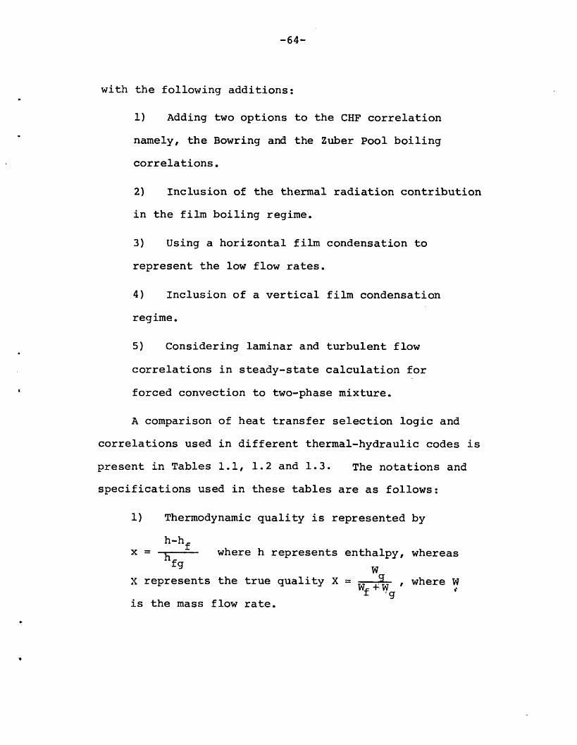
-64-
with the following additions:
1) Adding two options to the CHF correlation
namely, the Bowring and the Zuber Pool boiling
correlations.
2) Inclusion of the thermal radiation contribution
in the film boiling regime.
3) Using a horizontal film condensation to
represent the low flow rates.
4) Inclusion of a vertical film condensation
regime.
5) Considering laminar and turbulent flow
correlations in steady-state calculation for
forced convection to two-phase mixture.
A comparison of heat transfer selection logic and
correlations used in different thermal-hydraulic codes is
present in Tables 1.1, 1.2 and 1.3. The notations and
specifications used in these tables are as follows:
1) Thermodynamic quality is represented by
h-hfx =h where h represents enthalpy, whereas
fg W
X represents the true quality X = g where WWf+W 'Wfw r
is the mass flow rate.

-65-
2) The notations , Tw, Tf, Tat P,G represent
the void fraction, wall, fluid and saturated
temperatures, pressure and finally mass flux,
respectively. The dimension of the pressure and
mass flux are in terms of "Psia" and "lbm/hr-ft2
respectively.
3) The terms "High" and "Low" flow used in
these tables are in accordance with the flooding
correlation which read
1 1.-1 2
J + mJg = K [23]f g
where for turbulent flow m is equal to unity and
Jf and Jg are dimensionless velocities:
1 1* 2 2f = Jf f [ gD(pf-P g)]
f =J f1 [24]
Jg = J pg [gD (pf-pg)]
where D is pipe diameter and K is the flow criteria.
For example, in low flow region according to Ref. 40,
this criterion is
* 1 * 1Jf 2 - Jg 2 <1.36 for upflow
1[25]Jf 2 + Jg 7 <3.5 for downflowf 2 + Jg

-66-
4) The letter x and a in the parentheses in Table 3.2,
in front of the Thom and Schrock-Grossman correlations
imply that an interpolation is made with respect to the
quality and void fraction respectively, i.e. quality or
void fraction weighted heat transfer coefficient.
4. Fuel Rod Model
Temperature excursions of the fuel rod in case of any
transient or accident are a major point of concern in the
reactor safety analysis. A high temperature rise following
severe transients is a threat to the cladding material whose
integrity must be guaranteed in order to prevent any release
of radioactive materials. There are four barriers preventing
the release of radioactive fission gases to the environment
under normal operating conditions namely, the U02 fuel, the
fuel rod cladding, the reactor primary systems, and finally,
the reactor containment building (40). Accordingly fuel melting,
threatens the first barrier, and clad rupture violates the
second barrier. The ECCS final acceptance criteria requires
that failure of these barriers must be avoided under any
circumstances. This necessitates a realistic fuel rod
modeling, specially for the LOCA codes.
In general a fuel rod model consists of an approach
to solution of the general three dimensional, time dependent
H I O
(d O HsZ 4J
r0a)
04044
I Io )
W H )
O 0 d.,o .-I , ,
0 .~ ] -I P'
H -H-
I.
0 $ I *H
U
U >
0 0rZ U
r-IH00
P1
01)r--
- . H ::0 ( r--
4-) M rZ4
t
r-
C::·r11
I tt) r* *
U > 4 Cs-4 r 0 Cd 0 -'0 0-H .-I- -H N0 U4-)P4-
0)
a)5-40rux
) *rlI I
O H aU 4-) >
I d-> )
rl a) O rlrd r a 0) a) Q44JrLr4 0Z
I
> rGr
(
J I 1--I rl-Q) O 0O,.QOZ
I
U > s-IOO O -rT 4 4
,HJ43CdN
r-H
l-Ir-0
0
a)
Or- aH : d H
P 4
0)I E·I] I rl
, / a0 44
m/ u z
o
A lX
r0
A
0-
W* O
V V
vl v
H gO
r-i
ov
vo
o
o m; zo E
vI Al
Ep
0 Co ~1* z
o E ivl vx.
v pH
CN re) mo14 P0,P4 M 4
;·PI·
AL:
UL)0,-
o X
vI^ Al
0
LOo 0
LO XV (NP4 vI
U t o
A Al
a
0o Uo
A P4I-
4-J
a)-H
I
tC CdA 0)
U)
ov
v0o
0
ova-
U4J
EA
H
C)
EH
E-4V
Itr I Z
-iL ,¢ H lr > E4
x O H WIx O P
Ln
^l
0
H140
I4
mC
AIx
AC:A\4I
aI
Alx
3*H H
*.q W. 44
.00rl0"
HC0H
4)O aOI r
t0
tl)-i
E'
Cda)44
3:o0 H
tr O-.I ,-I":: rZ4
U)
Eqv
3Ev
E
Ln
ac l O
^Im5
ErC
A
3
Ln 4
oE Iv v >1
-3
o Cd1t (
o Hv v
H-4
I(a
~44-)MI
Int~03
Wt
4O I
O
A V
X 4dPL4
u
v
4-}CdI)
V
E
4-CdEn
o
oA
U]
vE-v
rZ4E-
4-rd
v
E- _
o
ov04
cn
o2=
H
Il;
I I II__ ___ __ __
-
____�___� -_I - - _L_ -
m I I I I
_ | --- - - -___
--- L I I IIpI i i __S-
- | -
-- -
-
I
II
I I I
I
I
I
i
I

-68-
o0
0d a)IJ U
fd *o< a
a) a) ErN k 5 4
E 5-4U U
H a5r: a
rd a,a) :.
I0)5-914
C04J
4.J Nro O-Ha) a) U >0
rd Ord) ) ()
4 >- Q) -rl3 r: ar-I rl
4- H > 0 -HC d a) Z o
a) a) a)
O O d
03 a C z m
o 0
4U -) rZro ( a)a) O)H . )
rX U CU
0)0
0 E
4-4P
4J
k c I(d C
*Q rQE: m9 m
4JaO
x m.- I
I rd i
o () amO O o
10 CdI O oX4 1 0
O 0k 5
E3 0O 00 0
4 p
E0
E-
a)
E-
4ard
"O
4 P4 P4
~4 ~-q c4w w 04 z z ;
Cd
U)00
O 0U)
zk
E0
0O0O
E-3
LO
HI
E mN' W o
ka,)
N O: IN -,
O * .-a z = S
.-1
4 -H 0Z-H Cbm
I
1a)H a
0 0-Hm H 0
U0a)
-H Oa >
a)C
a)
C11.u:
kI)I a) u4- a
r 44- 0-.,lQ
a)
G}
I a)024-)
4-) 0
.-
I
il
a-H.).,lu)
10 a4 0
C4
m
U)0o3
U
I-----"-
u
I > ~ ~ - I
-69-
a Oro -H
r4JO dU o
-I
a O
O rI .0 rd -
- I OU 4-
:d O- r.- W O Q
Z 0 -H >Z U 4) >
00r,4U
0
: UU) 0O C . a
4J m P: >
-lH SH
o H 0O- , O
U)U1
3O c4 P4
o U
U>
00rI
*H
H-L O* m
O H*H - -H,4J U)
roI
-H rd W)U) H
O Cd O MdHO k 4J (-PtE- c- uz
-H.I
0
-1O-
0m
I I t
O) OH H O4 0, d 0 -H
0 0 - ) -H 01
,- t11 rn
Im
U)
0
Ia)0
0)0OQ)
03:O0)U)
i 4
HI
H> pqO r
0i o
Iva
0U)
m:.0a)C4
I
O U Or
u0
tN" n' ~ 0 I HPC PN P4 e e , c H>
E)a)
q 4 )
.H
3 xI Cd
-tf +
N
Cdk
O
3H OO
m O
0 -H
0
4-I"U0)
o
rH0
k)
.. 3 I3 oO I *r C
- O ,0 O t0O -H 9>4 *(
PL . ___
Ic z
uL
.. -r
rd
ON,H
H ..
O H
U>
I
,
Ud 0U001
I
U)
U)
U"G
I k4
4U)
- OC m
r"-E
~3 o'O * k
0 . i .W1 -(aU) .
I
,H
t1)
0
g
H0s-I
o
rd
-4
'' W W I-
·I U-U) U Um
0.,,w 0 wI.. a 4.)
Z7 a 01 0
.H0 z-HS-l
-H
CD
E-H
C) 9
-,14r
WU)
H Oro
d dE- qW
0
U)
EnU)
tri.a,
q.01)
4-4U)
E-qCd
I C :03),
z I
U)0
_ - t _-------------- ------- C-;__.
_- -- -- ._--- ---�---�---------- -- -- -- ·- ---_
�^--LI-----------
i
i
I
iIii
I
II
I
l
.. /1 /'1

-70-
Poisson's equation (heat conduction equation)
p c - = ' (K VT) + Q"' [26]
where T,t,p and cp represent the temperature, time,
material density and specific heat respectively. In
this equation K represents the conductivity tensor,
K = Kij, i=1,2,3, j=1,2,3 and Q" is the heat source
density which represents the amount of heat generated
in the material per unit volume per unit time. Generally
as the cylindrical shape of fuel rod dictates, a cylin-
drical coordinate system is chosen to expand the first
term in the RHS of Equation 26.
4.1 Fuel Region
The expanded form of equation 24 in the fuel region
is:
T 1 a3T 1 3 aT ap r r
aT( k 3T) + Q [27]
where k in equation 25 is no longer a tensor but a
time dependent scaler. This simplification is made
possible through the valid assumption of homogeneous,

-71-
isotropic solid for U02 and fuel rod cladding material.
The first term in the right hand side of Equation 27 is
considered in the more general form in COBRA-IV-1 as
follows:
r - direction: 1 (r a- k DT
By assuming a=2, the cylindrical and a=l, the planar fuel
can be treated.
The total derivative in the left hand side of
Equation 26 is changed to a partial derivative in
Equation 27. This simplification is possible as long
as a stationary solid is treated. This in turn is a
valid assumption since the fuel centerline melting is
to be prohibited by design under any circumstances.
The azimuthal, or O-direction, conduction is ignored
in all the reviewed fuel rod models. This implies an
assumption of infinite circumferential heat conduction.
The axial conduction, Z-direction, is only considered
in COBRA- IV-1 and is ignored in the other codes.
Further simplification to Equation 27 is possible by
assuming that all physical properties are temperature
independent, in addition to the isotropic assumption. This
is done for example in WOSUB. However, the temperature

-72-
dependence of thermal conductivity and heat capacity
is considered in TRAC and THERMIT. The latter uses a
chebyshev polynomial fitted to the MATPRO(4 3
expressions which represent fits to experimental data
for fuel and clad material properties. For example a
cubic and a quadratic polynomial is used to fit the
temperature dependence of p, cp and k of the fuel,
respectively.
The Kirchoff's transofrmation is used in COBRA-IV-1
to reduce Equation 27 to a linear partial differential
equation. By using this method the temperature dependence
of k is taken into account.
As for the RELAP series, RELAP2, RELAP3, RELAP3B
and RELAP4 use a simplified lumped model for their heat
conduction calculation. In these codes heat generation
is determined by reactor kinetics routines or by input
specified values for power versus time. The fuel rod
model used in these codes is patterned after the model
used in the HEAT1 code. The final form of the heat
conduction equation is presented in Table 4.1, equation
28. In this equation, the average temperature is
defined by (11). n
_ pc TdV_ TVPd n =l(PV)n(Cp)n nn
/vPC dV E (pV) (cp)p n=l n n

-73-
where V and N represent the fuel volume and fuel pin
annulus number respectively. Also s in Equation 27 is
the fuel pin surface area.
Equation 27 representes the U-tube as well as once-
through steam generator modeled in RELAP3B-MOD101.
Naturally Equation 27 does not include any heat source
density term.
Equation 28 reflects the cartesian geometry used
in the RETRAN fuel rod model. Thermal conductivity and
heat source density temporal and spatial dependency are
accounted for.
In Table .1, Equation 31, Equation 32 and Equation
33 represent the COBRA IV-1, COBRA-III P, WOSUB, TRAC
and THERMIT, one dimensional heat conduction equation.
Thermal source density Q"' in COBRA-IIIC & COBRA-III P
is calculated as follows: The total power is
Q = D AZ Q" [35]
where D, AZ and Q" are the fuel rod diameter, the
axial interval and the heat flux respectively. Now
dividing by the fuel volume gives
Q' = Q" Z Q" 4D [36]I 2 -2
TDf Df
4- A Z

-74-
where Df represents the fuel pellet diameter.
The thermal source density in WOSUB is assumed to be
spatially uniform but time dependent, whereas in TRAC and
THERMIT it depends both on position and time. Equation 34
demonstrates the COBRA-IV-I fuel rod model. This equation
is found by using the Kirchoff's transformation.
0 k To k(T)dt [37]
where k is the conductivity at reference temperature
To . Differentiating Equation 37 with respect to r and t
and substituting in Equation 27 we will come up with
Equation 34.
4.2 Fuel-Clad Gap
The fuel-clad gap heat transfer coefficient is implicitly
treated in those models in which clad and the fuel-clad gap,
are lumped together.
This is done for example in the COBRA-IIIC fuel rod
model. However, upon the importance of the fuel-clad gap
resistance to the heat flow, it is treated explicitly in
RELAP3B-MOD101, WOSUB, TRAC and THERMIT.
The gap heat transfer coefficient depends upon the
fission gas product in the gap, the radiation heat

-75-
tJ1O
r.
0td *HCd )3z r-l wo u 1:
4-iC)0
ro
Cd
c:
-,
co(N
rH W4
r= H a X)
1-Q)Y
a Ir
U)
H 4 i +I '
H a) 0" II
E- : ) rlo 04-) , H
a
0U4J
0d ! 0O
X rj1 aO 4
4-). 4-)o : O
nl f Ii
C1)
rdi 1-1 .
IN
Er, 4
C1
0
UC
Hr
I -H 4
XO
C)·- a) rW C
Z dC Vsam Pc r/z~r ct a aI *,1
a HU1d
O
x-Iv
0r
4XX
E-
Co
0
00-M1)o EC _a)
U .-Hrda@a)I4-O4-i
,-t
tdH O
r rb ord rl )V O D4
- a)a W d 0 d p 0~Lm cc-
E-
C)4-)U"
rl.
H)Cd 4.
·-I 1.0
U )(o4-) QI U)H F
. 0
U IHH H, I* a) u)
HH
00
U UCC= I.,U)
(NC14m
0II
I-i
ii
+
Co
10
.-o 1*Iu I E
ardO
-H 4
) a)a
*H U) a)90.I .a Or
I
Io
4-) Oa) -H
-. 4-)r
+"--'
4-)1 k
E-4Co
4J
4-)-111
,0
r-
H
ro
U
I.-1a
E-E-
ro
oonl I
Ord o a)I C:
a) a)
- t0 ,C4-
-
En
-
+
I
td
CH
0 (0S
N
I I
I-E
01-)Q
* rdI V
OH
0H1C3:>
%- ,
Z 04
r'll

-76-
transfer across the gap as well as the fuel-clad
contact and fuel-clad pressing(20 . These are modeled
in the GAPCON, MATPRO, FRAP-S and FRAP-T codes. It's
MATPRO model which is implemented in THERMIT. In
this model all the above mentioned factors are considered.
The model used in TRAC ignores the effect of fuel pressing
against the clad, whereas it is correlated in THERMIT in
terms of the fuel contact pressure against the clad.
An effective gap heat transfer coefficient is used
in WOSUB. Although this is not as realistic as the models
used in TRAC and THERMIT, it still allows nodalization in
the clad. COBRA-IIIC and COBRA-IV-1 assume the outer
fuel surface and the inner clad surface are in a single
node. In this case the conduction equation is written
between the fuel and clad exterior surface. The heat
transfer coefficient used for this purpose is defined as(4)
1 1 1 YcH H k
g c
where Yc and kc are the cladding thickness and conductivity
and H is the fuel-clad gap conductance.
4.3 Clad Region
As mentioned in the previous section 4.2, only
WOSUB, TRAC and THERMIT permit clad nodalization. While

-77-
the clad region is assumed to be heat source free in
WOSUB, a metal-water reaction is considered as a heat
source in that region in the TRAC fuel rod model as
well as RELAP4. This reaction happens at elevated
temperatures, below the cladding material melting
point, between zirconium and steam and is expressed as :
Zr + 2H20 ZrO2 + 2H2 + Heat [38]
Both TRAC and RELAP4 use the parabolic rate low
of Baker and Just to represent the rate of this reaction
but in a different system of units + + The mathematical
statement of the parabolic rate low reads:
dr _ a bdt ( R Jr)exp(.
where r, Ro, t and T represent the radius at each
moment, the initial clad exterior radius, time and
temperature respectively. In this equation a and b are
constant values. By integrating Equation 39 between the
initial and final radii of a time step, the mass of
zirconium reacted per unit length during the time step
will be found, The amount of heat generated in the clad
is then proportional to this reacted mass, and it will be
considered as the internal heat source in the clad region.
+ This exothermic reaction, results in hydrogen gas whichposes a threat to the fuel rods in case of accidents byexcluding the upper part of the rods to be covered bythe coolant.
++ TRAC and THERMIT are the only thermal hydraulic codesusing the SI units.

-78-
5. Numerical Methods
The mathematical models which were discussed in the
previous sections are solved numerically in the computer
codes, because analytical solutions are impractical.
In the subchannel codes, the axial length of the
reactor core is divided into several intervals which
make each interval the computational control volume.
The set of field equations in a finite difference form in
conjunction with the constitutive equations are solved for
the central volumes. The boundary conditions at the inlet
of the core are, uniform or nonuniform pressure and coolant
densities and enthalpies. The axial and radial heat flux
profile must be specified. The solution is based on
reaching a uniform pressure at the core outlet. For this
purpose, a marching technique may be used. In a step by
step, or marching technique, the calculation starts from
the bottom of the core for all subchannels and moves upward.
Inlet velocities are first assumed to be known and then
solved alternatively through the external iteration loop.
At each axial node, the cross-flow is guessed which allows
solving the energy equation. A new value for cross-flow is
calculated from pressure drop in each subchannel, which
in turn is calculated from the momentum equation.

-79-
This internal iteration on cross-flow is continued
until an acceptable pressure balance is reached. By
knowing the heat addition into the axial cell and
calculated cross-flow for the axial cell, the values
of coolant density, velocity, enthalpy, and pressure
can be determined at the exit of each computational
cell. In turn, these values will be used as the
information for the next axial cell. This procedure
continues until the top of the core is reached where
the criterion of uniform exit pressure is checked. If
this criterion is not met, the external iteration loop
which covers the whole channel length must be continued,
using improved guesses of the flow division among the sub-
channels at the inlet. This procedure was employed in
COBRA-II and HAMBO. The number of external iterations
over the core length depends upon the coupling between
subchannels. If this is weak (e.g. if the cross-flows
are small), a single pass marching solution technique
is adequate (2 2 ) , otherwise a multipass marching solution
is necessary. This concept is used in COBRA-IIIC, in
which a pattern of subchannel boundary pressure
differentials for all mesh points is guessed simultaneously
and then the corresponding pattern of cross-flow is
completed using a marching technique up the channel. By
updating the pressure differentials during each external
-80-
iteration loop, the effects of downstream will be
propagated upstream.
The procedure used in COBRA-IIIP is somewhat
different. A new treatment is introduced for the
transverse momentum equation which couples the adjacent
computational cells. This includes the spatially semi-
implicit treatment of the pressure field.+ Using
this method guarantees the diagonal dominance of the
matrices governing the pressure fields(49) The computed
pressure field is then used in the transverse momentum
equation to determine the cross-flow distribution.
Applying the new concept in COBRA-IIIP has made it capable
of increasing the number of computational subchannels
markedly, i.e. from 15, in COBRA-IIIC, to 625 in
COBRA-IIIP (4 4 ). Furthermore, it has increased the compu-
tational effectiveness resulting in a shorter running
time. ++
By introducing a scalar, value 0, having an arbitraryvalue between 0 and 1 the pressure field is written:
[P] = [Pj] + (1-8) [Pj_l]
By introducing this concept into transverse momentumequation, allows the cross-flow distribution to be drivenby any combination of the pressure fields that existat the top and the bottom of each plane of computa'-tional cells.
Unlike COBRA-IIIC, a double precision is used in compu-tation of pressure field and gradients which is speciallypronounced in cross-flow distribution calculation in thevicinity of grids. This in turn will increase thecomputer running time.

-81-
While the marching technique determines the flow
condition under steady-state situations, in transients
the whole procedure will be repeated for each time
increment, implicitly in both COBRA-IIIC and
COBRA-IIIP. The marching technique is also employed in
WOSUB, where for the sake of numerical stability, a
backward finite difference form is used in space and
time. The lack of transverse equation and cross-flow
is compensated by the concept of recirculation loop
which is based on the assumption that the net volumetric
flow recirculation around closed loops connecting
(17)communicating subchannels is zero
Simultaneous solutions of the finite difference
form of the field equations written for the previously
defined computational cell, is another solution technique
used in some subchannel codes such as SABRE and COBRA-IV-1.
Since the calculated values will be advanced in each time
step explicitly, this additional option in COBRA-IV-1 be
called the "explicit solution scheme". The following
possibilities are available in COBRA-IV-1 solution
algorithm:
1) Steady-state and transient calculation using
the COBRA-IIIC implicit solution scheme.

-82-
2) Implicit steady-state and explicit transient
with either a AP or inlet flow boundary condition.
3) Explicit transient calculation based
specified initial values with either a AP or
inlet flow boundary condition and a zero flow
initially.
The addition of the explicit numerical scheme with
a AP boundary condition makes COBRA-IV-1 capable of
handling flow reversal, recirculation and coolant ex-
pulsions as well as severe flow blockage.
These additional capabilities stem from solving a
true boundary value problem rather then dealing with an
initial value problem in the marching type solution
technique.
The additional numerical scheme in conjunction with
the boiling curve package and the improved fuel pin-model
makes COBRA-IV-1 capable of assessing accidents such as
a LOCA, where due to the heat transfer package inability
of analysing reflood, the code capability limits to the
blowdown phase of a LOCA. It should be realized that due
to numerical instabilities and convergence difficulties
which mostly result from discontinuities introduced by
the physical models, the "explicit scheme" of COBRA-IV-1
uses the strict HEM, i.e., it does not contain the Levy
subcooled boiling model or any slip correlation. Further-
more the lack of computational effectiveness, as

-83-
compared to COBRA-IIIC and IIIP, and using the
reference pressure concept* which excludes any
effect of compressibility and also large heat flux
oscillations observed in prediction of depressuri-
zation transients(4 6 ) have made COBRA-IV-1 less
desirable. Overcoming these deficiencies has been
presumably the motivation of creating COBRA-DF and TF.
As for the loop codes, a fully implicit solution
scheme, temporally, is employed in all the RELAP series
as well as RETRAN. An automatic time step variation
is built in RELAP3B-MOD101. Using this feature, the
time-step size increases automatically during slowly
varying portions of a transient case of a computer run
and vise versa. Both implicit and explicit solution
schemes are employed in RETRAN.
Unlike the implicit method which is unconditionally
stable, the explicit method is conditionally stable
in which the so-called "courant criterion" must be
respected. This criterion reads:
AT AXU AX < I or AT < [40]
where U is fluid velocity, AT and AX are time step and
The concept of reference pressure which ignores the soundwave propagation effects is employed in all the HEMversions of COBRA as well as WOSUB. This limitation iscircumvented in COBRA-DF by using the ACE method, alsosee Ref. [45] in which this method is applied to theCOBRA-IV-1 field equations.

-84-
mesh spacing respectively. It is clear that for
fast transients which involve rapidly changing flow,
very small time steps may be needed to resolve the
flow evaluation. An explicit numerical scheme may
be used for this purpose.
Longer time steps are desirable in calculating
the mild transients, which necessitates using the
implicit numerical scheme. This scheme has not been
used in the three dimensional thermal hydraulic codes,
because, the fully implicit difference equations are
very difficult to solve in more than one space dimension.
A marching solution method may be applied to circumvent
this difficulty, but as it was discussed earlier, no
true boundary value problem can be handled by this
method, only initial value problems in which general
boundary conditions and local flow reversal cannot be
treated.
A compromise between the above mentioned techniques
has been made in THERMIT by using a "semi-implicit"
numerical scheme. As the name implies, both implicit
and explicit schemes are employed in such a way that by
differencing terms involving sonic propagation implicitly,
limitations (U±C)AT I <1 have been eliminated,'
whereas the liquid and vapor convection are treated
explicitly.
-85-
Therefore the limitation imposed on the time increment
to satisfy courant criteria (Equation 40) still exists. A
default value is usually built in the codes which use a
temporal explicit scheme to exclude the computational
instability.
6. Summary and Conclusions
6.1 Summary
A summary of the aforementioned methods and models used
in each reviewed code and the range of each code application
are presented in Table 6-1 through 6-5.
Some of the terms which are used in these tables are
further explained as follows:
Small breaks (Table 6-1): postulated breaks that
are smaller than about 10% of the double-ended
break in the discharge flow area.
Licensing codes (Table 6-1): notations are in
accordance with the notations defined in Table 6-3.
Homologous model (Table 6-4): described the
centrifugal pumps and specifies relations,
connections head, torque, flow rate, and rotational
speed.

-86-
Table 6-1
Component and Loop Codes Comparisons
TYPE APPLICATION CHARACTERISTICS
Code -I
Name O
H 4J . U)
X)X X O X l) 4m 0W W 43 1 I k U W M tl -i -i Q W U Hr d W 0 U U)
COBRA I XX X X X lVlT Ax i al Forward Steady aLateral March- State
ing
Axial Forward Steady 2COBRA II X X X X X X 1V1T Lateral March- State
ing
Axial Pseudo SteadyCOBRA III X X X X X X 1VlT Axial Pseudo Steady 3
Lateral Boundary StateCondi-tion
Axial Implicit SteadyCOBRA III-C X XX X X X 1V1T teral Stat 4
Lateral State & 4Transient
Semi-
Axial Implicit SteadyCOBRA III-P X X X X X X lVlT Forcing State 5
Function Transientforcrossflow
COBRA IV-I X XX X XX X lVSlT Axial Ilicit Steady 6Lateral Explicit State &
Transient
SteadyCOBRA-DF X X X X X X lVD1T State & 7
Transient
COBRA-TF XX X XXX 2V2TSteadyState & 8
Transient

-87-
Table 6-1
Component and Loop Codes(continued)
Comparisons
CodeName
WOSUB
THERMIT
RELAP2
RELAP3
RELAP3B(MOD101)
RELAP4
(2)RELAP4-EM
RELAP4-FLOOD
RELAP4 (MOD5)
RELAP4 (MOD6)
X
X
X
X
X
X
xXX
X
X
X
X
X
X
X
X
TYPE
zrL
CPQ
X
t
t7O.a)Uci)
X
X
X
X
X
X
X
-IJcU
U)
X
ci)m(Q)M9
X
X
x
X
X
X
X
X
X
-P
0C)aaU
X
X
X
APPLICATION
0"o
0OOrn
X
X
X
X
X
X
X
X
oCCo
q~
X
X
x
No diversion cross flow
In conjunction with TODEE
X
X
-4 -14HrdE-O)fl J)~
CHARACTERISTICS
u
>O,1a)
o5: 0
lVD1T
2V2T
lV1T
I II 1V1T
I |lVlT
XI I1V1TX I | lVlT
I 1V1T
fx Txl lVD1T
X X 1VD1T
, )
~4(D
o)0a)U
AxialLateral
3-Dx,y,z
LumpedParameters
Uci
z
ImnplicitForwardMarching
(1)
Semi-Implicit
Implicit
Lumpe d Inplicit
Lumped i . .Parameters IITplzcitLumped llctParametersLumped
Prameters Implicit
Lumped I c.tParametersLumped
Lumped ImplicitParameters I
LImplicitParameters i
(for PWR) and MOXY (for BWR) .
U)03rJ(dU
ATWS
¢)U
(D4a,ci)Qici)
17
20
9
10
11
12
15
36
13
14
-l
-l - w | l i - - w
i
II
i, I
: I ll l- -
i i

-88-
Table 6-1
Component and Loop Codes Comparisons(continued)
TYPE APPLICATION CHARACTERISTICS
4J
Code ti~H 4~ C) CDCode . -S4 z >1 C .Name - Hu a) 3 H o s C
:oW:- z o o a) 4 o J a z W d "a0 z r0 Wa)W J 4 Qq 34 l rd Z H M a a
4 W u M 1 u LH o J M r o r o o tH3 -.H ) o ir o Q)4 E k > o 3 0
P4 mQ _ m_ U) U M 5: u m : P4
RELAP4 (MOD7) X XX XX XX X X lVDlT Lumped Implicit 14Parameters
RELAP 5 X XX X XX X X 2VTkTsat 1-D mpli 16k sat Implicit
RETRAN XX X X X X X X 1VDS1T(1 ) l-D Implicit 18Explicit
TODEE X X X X XX 37
MOXY X X X X X 38
2V2T 3-D Semi-TRAC-P1 X X X XX X X 2 3-D 191VT T r, , z Implicit19
1Dynamic slip model from the two-fluid theory

-89-
Table 6-2
Models and Methods Used in Some
Thermal Hydraulic Codes
g I CAPABILITY OR MODEL
Conservation Equation
Homogeneous equilibriummodel, HEM(lV1T)
One dimensional mass,momentum, energy equation
CODE NAME
IBNWL1967
X
X
CORA I CPmRA m pRAI III
BWL BNWL1970 1971
X
X
X
X
Drift flux model
COBRAIIICBNWL1973
X
X
Separate continuity equa-tion for liquid and vaporphases
Separate momentum andenergy equation for liquidand vapor phases
Turbulent liquid-liquidmixing in the subcooledregion, in energy equation
Turbulent shear stress inmixture momentum equation
Numerical Scheme
Flow Solution-Steady State:
Marching method (forwardmarching)
Xi
II
i
i
ii
I
X
X XPseudo boundary valuemethod
10 True boundary value method
11 New treatment of transversemomentum equation
COB.A COBRA WSUBIIIP IV-I
I I
MIT ] BNWL MIT1977
X
1 It
I,
1976 1978
X X
X I
X
X,
THEPMIT
MIT1979
X
x
X
X
I
Ii
I i
IX
I:
I
X
X
x
1
2
3
4
5
6
7
8
9
.. *_. *
i
X
I
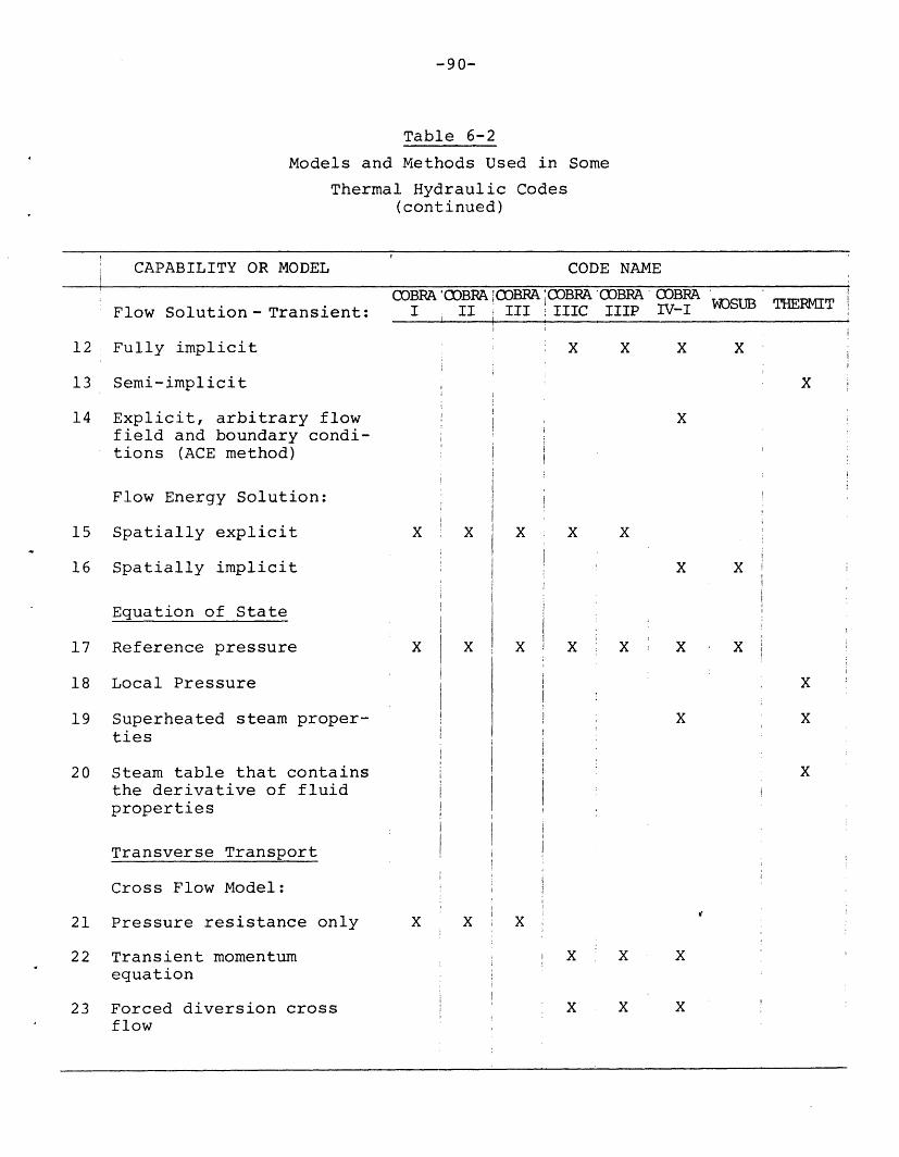
-90-
Table 6-2
Models and Methods Used in Some
Thermal Hydraulic Codes(continued)
CAPABILITY!~~~~~~~~ OR MODEL CODE NAMEt~~~~~~
CAPABILITY OR MODEL CODE NAME!1
Flow Solution- Transient:
12 Fully implicit
13 Semi-implicit
14 Explicit, arbitrary flowfield and boundary condi-tions (ACE method)
Flow Energy Solution:
15 Spatially explicit
16 Spatially implicit
Equation of State
17 Reference pressure
18 Local Pressure
19 Superheated steam proper-ties
20 Steam table that containsthe derivative of fluidproperties
Transverse Transport
Cross Flow Model:
21 Pressure resistance only
22 Transient momentumequation
23 Forced diversion crossflow
COBRA COBRA COBRA OBRA '0BRA COBRA I II III IIIC IIIP IV-I WSUB THE
i i
X X X X
X
X
X X
X; X X .
X X
X
X
X
X X
X X
X
X
X
X
X X
X X X
i

-91-
Table 6-2
Model and Methods Used in Some
Thermal Hydraulic Codes(continued)
CAPABILITY OR MODEL
Lateral momentum flux
Two dimensional transverseflow
Turbulent Mixing:
Single phase turbulentmixing
Two phase turbulentmixing
Vapor drift on a volumeto volume exchange basis
Accident Analysis
Severe flow blockage,coolant expulsion,reversal
flow
Recirculation loop
Single Phase Flow
Nonuniform channelfriction
Laminar and turbulentfriction correction
Hot wall frictioncorrection
Two Phase Flow
CODE NAME
ICOBRAII
COBRAIII
MRRA lCnOBRAIIIC
X
X
X
X
IIIP
X
X
X
X
COBRAIV-I
X
X
X
X
X
X
X
X
One-dimensional slip flow
241
s2b
261
27
28
29
30
31
32
33
WDSUB
X
X
X
X
X
X
X
THERMIT
X
X
X
X
X
X
X
- .
__ --_ _ _ _ ~ ~ - - I----" .-`--"..
II
iI
34 X X X X X

-92-
Table 6-2
Model and Methods Used in Some
Thermal Hydraulic Codes(continued)
CAPABILITY OR MODEL CODE NAME
COBRA 'COBRAI II
One-dimensional drift fluxmodel (Zuber-Findlay)
Three-dimensional (x,y,z)nonhomogeneous nonthermo-dynamic equilibrium flow
Subcooled voids (LevyModel)
Vapor generation rate termin subcooled boiling toaccount for thermodynamicnonequilibrium
Heat Transfer
CHF correlation
Boiling curve package
Heat Transfer RegimeSelection Tool:
Void fraction and CHF
Quality and enthalpy
Local clad surface temp.
Heat Conduction-Fluid:
Radial conduction
Axial conduction
Fuel Rod Model
Specified axial & radialheat flux
X
!
!
X i X~~~~~~~~~~~~~~~~~~~~
COBRAIII
X
X
X
COBPAIIIC
X
X
x
IIIP
X
X
X
IV-I U
X
X-
X
X
X
X
X
X
X
X
X
X
X
X
35
36
37
38
i
39
A q u
41
42
43
44
45
I
46
THERMIT
X
x I
x !
XXX
x
x
x
x
.
.. . ..
_ _ _ . _ _ _ _ _ _
lrnn'DA fflnD I_ " ^ . "'
It
I
IiiII
i
i
I
iI

-93-
Table 6-2
Models and Methods Used in Some
Thermal Hydraulic Codes(continued)
CAPABILITY OR MODEL
One-dimensional heat con-duction equ. (r-direc.)
Two-dimensional heat con-duction equ. (r,z-direc.)
Implicit finite differencesolution scheme
Collocation method
Orthogonal collocationtechnique (MWR)
Temperature dependentthermal conductivity
Transient (time dependent)heat source density
Constant fuel-clad gapheat transfer coefficient
Thermal radiation andinterfacial contact inthe gap heat transfercoefficient
Planar or cylindrical fuel
CODE NAME
COBRAI
COBRAII
COBPAIII
COBPAIIIC
X
X
X
COBRAIIIP
X
X
X
COBPAIV-I
X
X
X
X
X
Axial fuel zone
47
48
49
50
51
52
53
54
55
56
WOSUB
X
X
X
X
THERMIT
X
X
X
X
X
57 X
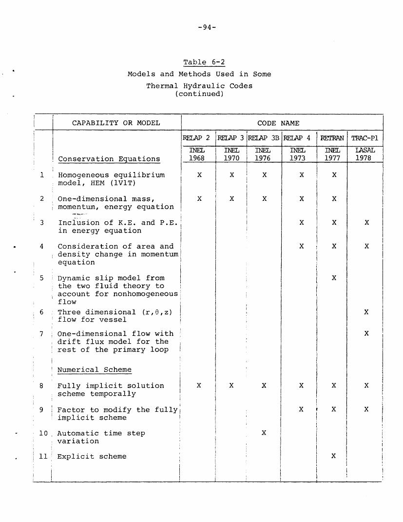
-94-
Table 6-2
Models and Methods Used in Some
Thermal Hydraulic Codes(continued)
CAPABILITY OR MODEL
1 .Homogeneous equilibriummodel, HEM (1VlT)
2 1 One-dimensional mass,momentum, energy equation
3 Inclusion of K.E. and P.E.in energy equation
4 Consideration of area anddensity change in momentumequation
5 Dynamic slip model fromthe two fluid theory toaccount for nonhomogeneous:flow
6 Three dimensional (r,9,z)flow for vessel
7 One-dimensional flow withdrift flux model for therest of the primary loop
Numerical Scheme
8 Fully implicit solutionscheme temporally
9 Factor to modify the fullyiimplicit scheme
10; Automatic time stepvariation
11 Explicit scheme
RELAP 2
INEL1968
X
X
X
CODE NAME
RELAP 3
INEL1970
X
REIAP 3B
IINEL1976
X
X i XX X
x 1xII I ,
X X
iIX
RELAP 4
INEL1973
X
X
X
X
X
X
TRAC-P1
LASAL1978
X
X
x
x
x
X
RTRAN
INEL1977
X
X
X
X
X
X
X
X
I_w .. -- .-
; (If- n -n V- 7n ' i n Pf-T I n+- i 'n
i
I
iI
I '.. . I, _
I

-95-
Table 6-2
Models and Methods Used in Some
Thermal Hydraulic Codes(continued)
CAPABILITY OR MODEL
Equation of State
Local Pressure
Steam table that containsthe derivative of fluidproperties
Extension of the steamtable above the criticalpressure
Physical Model
Pump Characteristics:
Homologous pump
Only one pump coastdowncurve
Independent tripping onthe independent signals
Pump is at a junction
Pump is in a volume
Consideration of inertialeffect
Consideration of friction-al torque
Consideration of bearingand windage torque
Option for two phase pump
Motor torque option, pumpstop option, & dimension-less head ratio differencedata in two phase pump
CODE NAME
RELAP 2 RELAP 3
X
X
X
RELAP 3B
X
X
X
X
X
RELAP 4
X
X
X
X
X
X
X
X
12
13
14
15
16
17
18
19
20
21
22
23
24
EKt'XAN
X
X
X
X
X
X
X
X
T1' U- A I
X
X
X
X
X
X
X
X
i _
i
. . .
I

-96-
Table 6-2
Models and Methods Used in Some
Thermal Hydraulic Codes(continued)
ICAPABILITY OR MODEL
Choked Flow:
M- 57 WI cAh . J luJuy a L.w.-jrllaz: .I.I.U
flow model
zb tienry-FtausKe ana extenaeHenry-Fauske
27 Sonic choking
Heat Exchanger:
28 Non-conduction model(input specified secondarytemperature & a constanteffective heat transfercoefficient)
29 Time dependent heat
exchanger (Input specifiedj table of normalized powerversus time)
30 Time dependent secondarytemperature
31i U-tube steam generator (onedimension heat conductionequation)
32 Once through steamgenerator
jSingle Phase Friction!Factor:
33 Laminar friction factor
34 Turbulent friction factor
35: Input specified frictionIr ,i
iUUI;
CODE NAME I
RELAP 2 IRELAP 3
V , V
X
X X
X X
RELAP 4
V
X
X
X
RELAP 3B
v
X
X
X
X
RETRAN
v
X
X
X
X
X
X
X
X
X ~i ~ ~~ [ ....j~~~~~i
X
X
i I
1I I
1) C
rI n r t
� I
i
i
.n 111. JX
I
. 1 1 I. - __ _ _ -1 - _ _- .- _
:
I
I
i
i
I
ii
I
I
_---- --
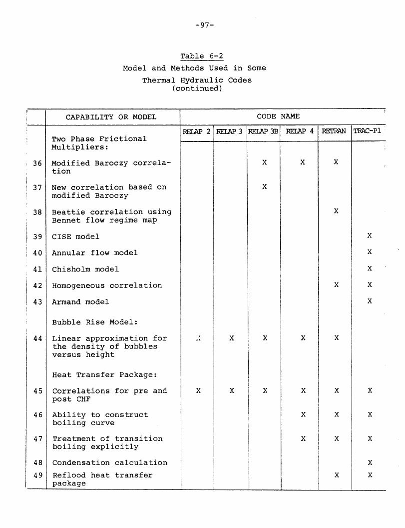
-97-
Table 6-2
Model and Methods Used in Some
Thermal Hydraulic Codes(continued)
CAPABILITY OR MODEL
Two Phase FrictionalMultipliers:
Modified Baroczy correla-tion
New correlation based onmodified Baroczy
Beattie correlation usingBennet flow regime map
CISE model
Annular flow model
Chisholm model
Homogeneous correlation
Armand model
Bubble Rise Model:
Linear approximation forthe density of bubblesversus height
Heat Transfer Package:
Correlations for pre andpost CHF
Ability to constructboiling curve
Treatment of transitionboiling explicitly
Condensation calculation
Reflood heat transferpackage
CODE NAME
REJAP 2
X
RAP 3 RELAP 3B
X
X
X
X
X
X
REAP 4
X
X
X
X
X
36
37
38
39
40
41
42
43
44
45
46
47
48
49
RETRAN
X
X
X
X
X
X
X
X
TRAC-P1
X
X
X
X
X
X
X
X
X
X
i
-
. . II
i
- -- / - -

-98-
Table 6-2
Model and Methods Used in Some
Thermal Hydraulic Codes(continued)
CAPABILITY OR MODEL
Heat Transfer RegimeSelection Tool:
50' Quality and CHF
51 Void fraction and CHF
CODE NAME
RELAP 2
X
b5z Local caa surface temp.
Fuel Rod Model:
53 Lumped approach X
J1- 54, One-dimensional heat
conduction equation
551 Variable gap size duringa transient
56 Thermal radiation andinterfacial contact in thegap heat transfercoefficient
57 Fuel-clad gap heat trans-fer coefficient burn updependent
58 Thermal conductivitytemperature dependent
59! Exothermic metal-waterreaction considered as aheat source in thecladding material
60 Explicit numerical scheme
61 i Implicit numerical scheme X
REAP 3
X
X
X
RELAP 3B
X
X
X
X
RELAP 4
X
X
X
X
X
X
RETRAN
X
X
X
X
X
X
TRAC-P1
x
X
X
x IX
Jr
-- - - --- -;
T-- - -
,, .,~~~~~~~~~~~~~~~~~~~~~~~ ~~ ~~~~~~~~~~~~~~~~~~~~~~~~~~~~~~~~~~~~~~~~~~~~~~~~~~~~~~~~~~~~~~~~~~~~~~~~~~

-99-
lI
ko
co4)Hd

-100-
6.2 Conclusions
A study was made of a number of well-known thermal
hydraulic codes. This study attempted to cover both models
and methods used in these codes summarizing their basic
elements in various tables. The following results are
drawn:
6.2.1 Component Code
The COBRA series as well as WOSUB and THERMIT fall
in this category. As for the COBRA codes, the steady-state
versions namely COBRA-I, II, III are certainly obsolete by
now and are not suggested for further considerations.
COBRA-IIIC and its MIT version COBRA-IIIC/MIT*, which
utilize the HEM model of two-phase flow, can be used for
both normal operation and transient conditions. The great
flexibility of COBRA-IIIC/MIT to simulate core regions,
bundles and subchannels at the same time, makes it more
desirable to use. An alternative marching solution using
implicit numerical scheme, which converges on the cross-flow
is used in this code. The fuel rod model in conjunction with
Pre-CHF heat transfer correlations make it a fast running
code for steady-state as well as mild transients. On the
other hand COBRA-IIIP/MIT is capable of handling a larger
number of computational subchannels with considerable computa-
tional effectiveness, since it deals with the diagonally
*The major difference between these two codes is that thelatter uses a dynamic data management subroutine which allowsthe dimensions of the principal arrays as well as the totalcomputer storage requirement to be a function of theproblem size.

dominant pressure matrix. However it should be realized
that these codes, COBRA-IIIC/MIT and IIIP/MIT, are not
devised for the purpose of accident analysis such as a
LOCA. In fact neither the physical models nor the numerical
methods have such capability. For example, lack of a heat
transfer package and use of the marching solution technique
do not allow any extreme flow as well as reliable fuel rod
temperature calculations. A step toward the analysis of
severe transients and/or accidents is taken in COBRA-IV-I
in which more realistic physical models, with respect to
the 2-D fuel rod model and heat transfer package, are
implemented. More importantly, a field equation solution
technique, explicit solution, is employed in addition to
the COBRA-IIIC implicit type solution scheme. It is
the simultaneous set of differential equations using
explicit solution technique which makes COBRA-IV-I capable
of handling severe flow blockages, flow reversal, coolant
expulsions and other extreme flow situations. Also, the
field equations solution using ACE technique allows
specifying a AP boundary condition which relaxes the
impractical specification of inlet flow boundary condition
in severe transients such as blowdown.

-102-
Despite these advantages, it should be recalled that
several disadvantages are associated with this code which
are as follows:
1) It relies extensively on the HEM,
2) Computational ineffectiveness,
3) The time change of local pressure is ignored,
4) Subcooled void is excluded in the explicit scheme.
A more realistic two-phase flow model that relaxes
the assumption of the HEM is used in the newer versions
of COBRA namely, COBRA-DF and TF, still under development.
Except for the highlights of the models used in these codes
that are presented in the summary tables, there is
little additional information available on these codes
for the time being.
Since analysis of the BWR normal operation and
transient conditions is more demanding with respect to the
two-phase flow modeling, the recent efforts in the BWR
models have been focused on using more realistic assumptions
with regard to vapor-liquid momentum exchange, or phase
distribution as for example the WOSUB code.
-103-
Unfortunately, the marching type solution
technique, simplifying assumptions such as the reference
pressure concept and lack of a complete boiling curve
package, in the current WOSUB version, put a limit on
its application. For example, no reliable blowdown
calculations can be performed with WOSUB in its present
form. Furthermore, WOSUB is not supposed to be used
for very fast transients.
It is now clear that extreme flow situations which
are a point of concern in severe transients can only
be evaluated by using more physically accurate field
equations. The two-fluid concept provides the potential
for increased accuracy in modeling the two-phase flow.
By implementing this concept in the most recent codes,
such as THERMIT, a number of limitations imposed on the
flow characteristics are relaxed. Now the motion of
two-phase in different directions, having different
temperatures, velocity and pressure can be realistically
analysed in three dimensions. The best estimate heat
transfer package, BEEST, and an improved fuel rod model,
specially with respect to the material temperature
dependent and fuel-clad gap modeling, which are included
in THERMIT, provide a reliable fuel rod temperature
calculation and DNBR prediction. A semi-implicit numerical

-104-
method is used to circumvent the instabilities
associated with the explicit numerical scheme.
In spite of the above mentioned advantages, it
should be remembered (see section 1.3) that the need
for mathematical models representing physical phenomena
increases with the degree of sophistication of the two-
phase flow modeling. Furthermore, the difficulty with
the general two-fluid approach is that the exchange
processes coupling the phases are currently not thoroughly
understood [ As a result, despite the possible
shortcoming of the HEM, it is not evident that a
homogeneous equilibrium model is incapable of predicting
adequately some parameters of interest such as vapor
flow rate and fuel-clad temperature. Furthermore, in
some flow regimes HEM gives surprisingly good results.
Therefore, as a final conclusion, for normal operation
and mild transients, COBRA-IIIC/MIT and COBRA-IIIP/MIT
are still the best available tools. Several shortcomings
of these codes such as the fuel-rod model and lack of
a heat transfer package and the like may be overcomed
by implementing the state-of-the-art models used in the
sophisticated codes such as THERMIT. Severe transients
and accident analysis are certainly advised to be aalysed
by THERMIT. Upon the completion of a subchannelwise
version with coolant centered control volume, THERMIT will

-105-
be the first three dimensional non-homogeneous fully
thermodynamic non-equilibrium subchannel code for the
nuclear reactor core thermal hydraulic analysis.
6.2.2 Loop Codes
The RELAP series as well as RETRAN and TRAC fall
in this category. The old versions of RELAP such as
RELAP2, and most of the RELAP3 versions are obsolete
and need not be further considered. RELAP3B-MOD101 is
the only updated version which uses several options for
heat exchanger and steam-generator modeling, not even
used in TRAC. This version is specially devised for
the ATWS analysis. It uses a combination of old models
of RELAP3 such as heat transfer package, and new models
introduced in RELAP4, such as homologous pump, in
addition to several unique features such as variable
gap size during a transient and heat exchanger modeling.
In light of the detailed information about RELAP4/MOD6
and MOD7 and RELAP5, the available highlights of loop
modeling are presented in the related tables. From
these tables it is clear that the major step toward the
non-homogeneous non-equilibrium modeling of the primary
loop is taken in the model making process of RELAP5.
Such effort is also done in RETRAN through introducing

-106-
the unique feature, DSM, "dynamic slip model". RETRAN
is specially devised to analyse the reflood phase of
a LOCA. The state-of-the-art of the loop codes however
is TRAC which is capable of handling all the phases of
a hypothetical LOCA.
As a result the following codes are suggested for
the transient loop calculations. First, RELAP3B-101
which is a one-dimensional, HEM code and it may be
used for ATWS transients. Second, RETRAN which uses
l-D, DSM and improved physical models, third, TRAC which
uses l-D, DFM for the loop calculations, and realistic
physical models.

-107-
REFERENCES
1. D.S. Rowe, "Cross-Flow Mixing Between Parallel FlowChannels During Boiling, Part 1: COBRA: ComputerProgram for Constant Boiling in Rod Arrays", BNWL-371 Pt. 1, Pacific Northwest Laboratory (1967).
2. D.S. Rowe, "COBRA II: A Digital Computer Programfor Thermal Hydraulic Subchannel Analysis of RodBundle Nuclear Fuel Elements". BNWL-1229, PacificNorthwest Laboratory (1970).
3. D.S. Rowe, "COBRA III: A Digital Computer Programfor Steady-State and Transient Thermal HydraulicAnalysis of Rod Bundle Nuclear Fuel Elements",BNWL-B-82, Pacific Northwest Laboratory (1972).
4. D.S. Rowe, "COBRA IIIC: A Digital Computer Programfor Steady-State and Transient Thermal Analysisof Rod Cundle Nuclear Fuel Elements", BNWL-1695,Pacific Northwest Laboratory (1973).
5. R.E. Masterson, "Improved MultidimensionalNumerical Methods for the Steady-State andTransient Thermal Hydraulic Analysis of FuelPin Bundles and Nuclear Reactor Cores", Ph.D.Thesis, MIT (1977).
6. C.L. Wheeler, et al., "COBRA-IV-I: An InterimVersion of COBRA for Thermal Hydraulic Analysis ofRod Bundle Nuclear Fuel Elements and Cores",BNWL-1962, Pacific Northwest Laboratory (1976).
7. C.A. McMonagle, et al., "COBRA Code Development",Fifth Water Reactor Safety Research InformationMeeting (1977).
8. M.J. Thurgood, et al., "COBRA-TF Development",Sixth Water Reactor Safety Research InformationMeeting (1977).
9. K.V. Moore and W.H. Rettig, "RELAP2 - A DigitalProgram for Reactor Blowdown and Power ExcursionAnalysis", 1D0-17262 (1968).
-108-
10. K.V. Moore and W.H. Rettig, et al., "RELAP3 -A Computer Program for Reactor BlowdownAnalysis", IN-1321 (1970).
11. - , "User's Manual for RELAP3B-MOD101, A
Reactor System Transient Code", NUREG-0004(1976).
12. K.V. Moore and W.H. Rettig, "RELAP4 - A ComputerFor Transient Thermal-Hydraulic Analysis",ANCR-1127 (1973).
13. C.E. Slater, et al., "Small Break AnalysisModels in RELAP-4 Computer Code", ANS Trans.Volume 22 (1975).
14. K.R. Katsma, "RELAP4 (MOD6 and MOD7), LWRReflood Code Development and Verification,Fifth Water Reactor Safety Research InformationMeeting (1977).
15. WREM: Water Reactor Evaluation Model, NUREG-
75/056 (Rev.l), Nuclear Regulatory Commission(1975).
16. V.H. Ransom, et al., "RELAP5 Code Developmentand Results, Fifth Water Reactor Safety ResearchInformation Meeting" (1977).
17. L. Wolf, et al., "WOSUB, A Subchannel Code forSteady-State and Transient Thermal-HydraulicAnalysis of BWR Fuel Pin Bundles, Volume I",M.I.T. Energy Lab. Electric Power Program (1978).
18. K.V. Moore, et al., "RETRAN-A Program for One-Dimensional Transient Thermal-Hydraulic Analysisof Complex Fluid Flow Systems", EPRI NP-408(1977).
19. - , "TRAC-Pl: An Advanced Best Estimate Computer
Program for PWR LOCA Analysis", NUREG 1CR-0063(1978).
20. W.H. Reed and H.B. Stewart, "THERMIT: A ComputerProgram for Three-Dimensional Thermal-HydraulicAnalysis of Light Water Reactor Cores", UnpublishedDraft of an EPRI Report.
-109-
21. W.T. Sha, "A Summary of Methods Used in Rod-Bundle Thermal-Hydraulic Analysis", Presentedto the Meeting Sponsored by the NATO AdvancedStudy Institute, Instanbul, Turkey (1978).
22. J. Weisman and R.W. Bowring, "Methods forDetailed Thermal and Hydraulic Analysis ofWater-Cooled Reactors", Nuclear Science andEngineering 57, 255-276 (1975).
23. G.P. Gasspari, et al., "Same Considerationon Critical Heat Flux in Rod Clusters inAnnular Dispersed Vertical Upward Two PhaseFlow", 4th Intern. Conf. Heat Transfer,Paris (1970), also Energio Nucleare, 17,643 (1977).
24. N.E. Todreas, "Analysis of Reactor Fuel RodAssembles Isolated Cell, Distributed ParameterAnalysis Appraoch", Class Notes at M.I.T.Unpublished.
25. N.E. Todreas, et al., "Single Phase TransportWithin Bare Road Arrays at Laminar, Transitionand Turbulent Flow Condition", Nuclear Engineeringand Design, Volume 30 (1974).
26. S. Fabic, "Review of Existing Codes for Loss-of-Cooland Accident Analysis", The Advances inthe Nuclaer Science and Technology, Vol. 10, 1977.
27. R.T. Lahey, F.J. Moody,"The Thermal-Hydraulicsof a Boiling Water Nuclear Reactor, ANS MonographSeries (1977).
28. F. Seifaee, "An Improved Numerical Method forthe Steady-State and Transient Thermal-HydraulicAnalysis of Fast Breeder Reactor Fuel PinBundles", M.I.T. Nuclear Engineering Department,NE Thesis (1978).
29. C.W. Stewart, "COBRA-IV: The Model and theMethod", BNWL-2214, NRC-4 (1977).
30. C.W. Solbrig and D.J. Barnum,"The RELAP4 ComputerCode: Part 1. Application to Nuclear Power - PlantAnalysis," Nuclear Safety. Vol. 17, No. 2 (1976).

-110-
31. W. Wulff, et al., "Development of a Computer Codefor Thermal Hydraulics of Reactors (THOR)", SixthQuarterly Progress Report, BNL-NUREG-50569 (1978).
32. - , "Multi-Fluid Models for Transient Two-PhaseFlow ", NP-618-SR (1978).
33. M. Ishii, "Thermo-Fluid Dynamics Theory of Two-Phase Flow, Eyro Ues (1975).
34. Y.Y. Hsu and R.W. Graham, "Transient Processesin Boiling and Two-Phase Systems", McGraw Hill(1978).
35. 10 CFR Part 50, "Acceptance Criteria for EmergencyCore Cooling System for Light Water-Cooled NuclearPower Plants", Federal Register, Vol. 39, No. 3(1974).
36. "WREM: Water Reactor Evaluation Model, Revision 1",Division of Technical Review, Nuclear RegulatoryCommission, NUREG-751056 (1975).
37. G.N. Lauben, "TOODEE2, A Two-Dimensional TimeDependent Fuel Element Thermal Analysis Program",NRC (1975).
38. D.R. Evans, "MOXY: A Digital Computer Code for CoreHeat Transfer Analysis", IN-1392 (1970).
39. W. Kirchner and P. Griffith, "Reflood Heat Transferin a Light Water Reactor", AICHE SYMPOSIUM SERIESNo. 164, Vol. 73.
40. T.A. Bornard, "Blowdown Heat Transfer In a PressurizedWater Reactor", Nuclear Engineering Department,M.I.T., Ph.D. Thesis (1977).
41. W.L. Kirchner, "Reflood Heat Transfer In a LightWater Reactor", U.S. Nuclear Regulatory Commissionreport NUREG-0106 (1976).
42. J.G. Collier, "Convective Boiling and Condensation",McGraw Hill (1972).
43. "MATPRO-Version 09: A Handbook of MaterialsProperties for Use in the Analysis of Light WaterReactor Fuel Rod Behavior", Idaho National EngineeringLaboratory report TREE-NUREG-1005 (1976).

-111-
44. L. Wolf and R. Masterson,"An Efficient Multi-dimensional Numerical Method for the Thermal-Hydraulic Analysis of Nuclear Reactor Cores",Nuclear Engineering Department, M.I.T., Tucson,Arizona (1977).
45. L. Wolf, et al., "Review of Iterative SolutionMethods for Pressure-Drop Forced BWR CoreAnalyses", Nuclear Engineering Department,M.I.T. (1977).
46. M. Massoud, "Comparison of Conservative andBest Estimate Heat Transfer Packages withCOBRA-IV-I", Nuclear Engineering Department,N.E. Thesis (1978).
47. Z. Rouhani, Chapter 14 of "Two-Phase Flows andHeat Transfer with Application to Nuclear ReactorDesign Problsms", edited by J.J. Ginoux,Hemisphere Publishing Corporation.
48. N.E. Todreas, class notes, Department of NuclearEngineering, M.I.T.


-112-
APPENDIX 1
In the following, the assumptions which have been made
in derivation of the continuity equation in the COBRA codes
are discussed.
The mass balance for liquid is given by:
a I (1 )at [(l-a)pl] + V [(l-a)p1 f1 ] = -r (
Mass balance for vapor follows
at [(Pv ) ] + V'[(PvV)]= (2)
where r is the phase change rate. Now using a pseudo
single phase concept by assuming:
p = (l-a)p + (3)(3)
pV = (l-a)p1 V + Pvv
and adding terms (1) and (2) we will come up with
at ) pl + (p)] + V[(1-)pV l + Pv v] =
Now using the "averaged values" introduced in (3) in the
equation (4), we will come up with the single phase mass
balance
at( + V V) = 0 (5): 0 , (5)at
Equation (5) in a more involved form becomes:

-113-
a at(pddxdz)dx + ay(pdxdydz) + (pVdxdz)dy +t DX DY
(6)
" (pVdxdy)dz = 0
where the element of volume, dn dy dz, represents the control
volume used.
.pVxdydz
z
dz
PVxdydz+ (pVxdydz)dx
dy Fig (1)
Now in equation (6) by eliminating dz we'll have:
ata(pF- (dxdy) + (Vdxdy) +dxdy) + (pVdydx)=
In equation (7) if we assume that the control volume
(7)
shown
in Fig. (1) has only an infinitesimal height, dz, and its
cross section normal to the z-axis "finite" instead of
"infinitesimal" (i.e., dxdy A , we will come up with:
A) + t((pVA) + (pVA) + (PVA) = 0Dt 9z au DX (8)
and by substituting pVA = m we have:
a +t(pA ) + -(m) + ) + a(m)= at ~ -9a ay (9)
A "subchannel control volume" concept used in COBRA
assumes a finite cross section normal to the z-axis which

-114-
has the same area, A, equal to the physical subchannel size,
and an infinitesimal height, dz.t
Idz dz
w . = .1] 31
Aide tpvA [wi ] = lbm/hr-ftLde I OVAfuel t facerod
Fig (2)
In Fig. (3), w*ij represents the 'cross flow" concept. Mass
balance written for control volume shown in Fig. (3) becomes:
d dpVA + T-(pVA)dz + w* .dz - pVA = - (pAdz)dz 13 dt
d ddt(pA) + (pVA) + w* = 0 m = pVA (10)
Comparing equation (10), used in HEM versions of COBRA, with
the pseudo single phase continuity equation, equation (9), we
conclude that the cross flow term w*ij represents the two
dimensional form of mass flow rate per unit length, i.e.,
(- + )m + w*. (11)ax ay ij
Flow Blockage:
This phenomena is only considered in COBRA-IV-I. None
of the remaining HEM versions of COBRA account for this
tThis infinitesimal length becomes the axial interval betweenthe selected axial mesh points in the finite differencesolution technique.
t,_j --�,
a- .p VA CL

-115-
feature. Therefore in these versions, i.e. COBRA III and
COBRA III-C and ..., equation (10) is simplified by assuming
aA 0at 0
A dp + p d(m) + w*.. = 0dt + dz +
aP. am. NA + i - C w* (12)
Ai t ax ij
where the subscript i represents the subchannel under
consideration.
Rewriting again equation (11):
d -- d NAdt p + -(pV)A + YW = 0 (11)
dt dz j=l
where in this equation, the averaged values are emphasized by
using a (-) sign. This in fact follows using an integral
form of mass equation which reads
at fTpdT + Jsp( · n)dA = 0 (12)
where T, s and v represent volume, surface and velocity
respectively.
Define the volume and surface averaged values for
density and mass flux:
1p = <<p>> = - f pdT
(13)
pV = <pV> = I f p(v . )dA
where V = TdT and A = fsdA . Also one bracket show area
averaged and two bracket shows a volume averaged value.

-116-
Evaluating equation (12) for the control volume shown in
Fig. 2 we have
V P + VAlupper face - VA Ilower face (w )bz = O (14)
where w sie p(v n)dA and V = A-Az
faces (15)
If Az becomes small, in limit we will have equation (11).


-117-
APPENDIX 2
The details of the correlations introduced in Tables
3-1 to 3-3 are presented here.
1. Pre-CHF Heat Transfer Correlations
The heat transfer correlations used in the pre-CHF
heat transfer regimes are as follows:
Dittus-Bolter(A-l) correlation:,Gh 0.GDh 0.8
h = 0.023(-) Cpp 0.4k
* kDh
.... Data Base:
GDhRe = - greater than 10,000
Pr - 0.7 to 100
LDh greater than 50h
Sieder-Tate ) correlation:
GDh 0.8h = 0.023(-)
1.
(Cpp 0.4 * k . ( )0.14
Dh
Data Base:
As for Dittus-Boelter correlation.
Thom correlation(A-3):
P 1
T = T + 0.072 e 1260w sat w
Data Base:
Vertical upflow of water
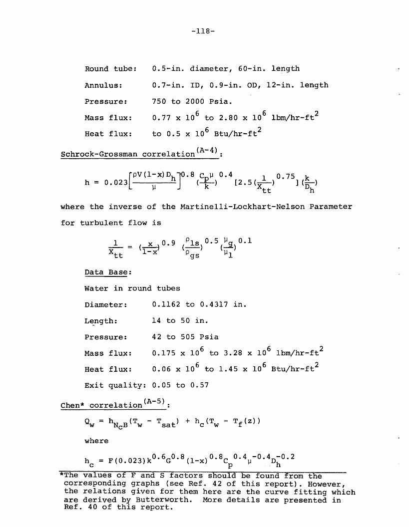
-118-
Round tube: 0.5-in. diameter, 60-in. length
Annulus: 0.7-in. ID, 0.9-in. OD, 12-in. length
Pressure: 750 to 2000 Psia.
Mass flux: 0.77 x 10⁶ to 2.80 x 10⁶ lbm/hr-ft2
Heat flux: to 0.5 x 10⁶ Btu/hr-ft2
Schrock-Grossman correlation(A-4):
rPV(l-x)Dh1O.8 C p1 0.4 1 0.75 kh = 0.023L (- -) [2.5(X ) ]( )
where the inverse of the Martinelli-Lockhart-Nelson Parameter
for turbulent flow is
1- x %0.9 Pls 0.5 P( 0.1
tt gs
Data Base:
Water in round tubes
Diameter: 0.1162 to 0.4317 in.
Length: 14 to 50 in.
Pressure: 42 to 505 Psia
Mass flux: 0.175 x 10⁶ to 3.28 x 10⁶ lbm/hr-ft2
Heat flux: 0.06 x 10⁶ to 1.45 x 10⁶ Btu/hr-ft 2
Exit quality: 0.05 to 0.57
Chen* correlation( A- 5):
Qw =hNB (Tw- Tsat) + hc(Tw- Tf(Z))
where
hc F(.023)k0.6G 08 (l-x)0.8c 0.4 -0.4 -0.2C p 'P p h
*The values of F and S factors should be found from thecorresponding graphs (see Ref. 42 of this report). However,the relations given for them here are the curve fitting whichare derived by Butterworth. More details are presented inRef. 40 of this report.
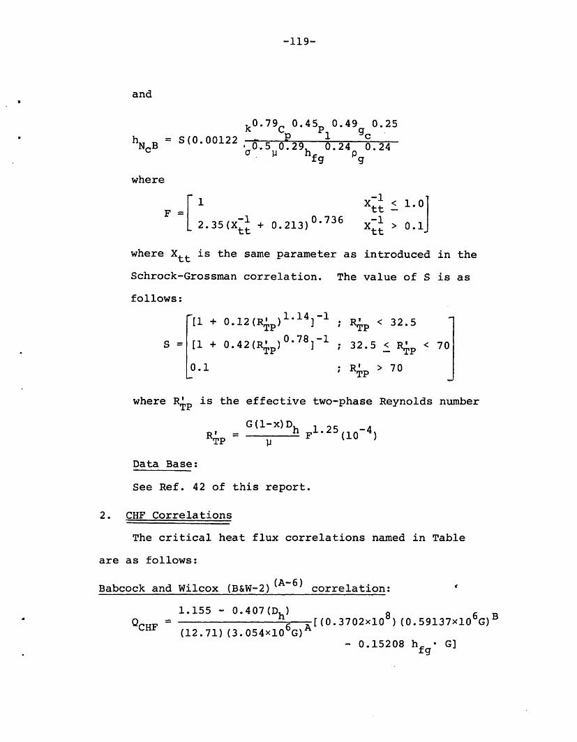
-119-
and
k0.79C 0.45p 0.49 0.25
h = 5(0.00122 - p 1 ChNcB = S(0.05 0.29h 0.24 0.24
w1heefg Pg
where
F = -1 0.736L 2.35(Xtt + 0.213)
Xt1 < 1.0tt
X > 0.1
where Xtt is the same parameter as introduced in the
Schrock-Grossman correlation. The value of S is as
follows:
[1 + 0.12(Rp)l.14]-
S = [1 + 0.42(Rp) 0.78 ]-
0.1
; Rp < 32.5
; 32.5 < R p <
; Rp > 70
where RTp is the effective two-phase Reynolds number
G(l-x)Dh 1.25 (10-4
Data Base:
See Ref. 42 of this report.
2. CHF Correlations
The critical heat flux correlations named in Table
are as follows:
Babcock and Wilcox (B&W-2)(A6) correlation:
1.155 - 0.4 07 (Dh) 8Q = A[(0.370 2xl ) (0.59137x1 06 G)B
CHF (12.71) (3.054x10⁶G)- 0.15208 hgs G]
70

-120-
where
A = 0.71186 + (2.0729 x 10 ) · (P - ]000)
and
-4B = 0.834 + (6.8479 x 10 ) (P - 2000)
Data Base:
Vertical upflow of water in rod bundles
Heated equivalent diameter of subchannels: 0.20 to 0.50 in.
Heated length: 72 in.
Pressure: 2000 to 2400 Psia
Mass flux: 0.75 x 10⁶ to 4.0 x 10⁶ lbm/hr-ft2
Thermodynamic quality: -0.03 to 0.20
Uniform axial flux distribution.
Westinghouse (W-3) (A-7) correlation:
QCHF = {[2.02 - 0.430(0.001P)] + [0.172 - 0.000]P
exp[18.2x - 0.00413P-x]}(1.16 - 0.87x)
[(0.148 - 1.6x + 0.173xlxl) (G/106) + 1.04]
[0.266 + 0.836 exp(-3.15Dh)]
[0.826 + 0.0008(ht - h i )]10
Data Base:
Diameter: 0.2 to 0.7 in.
Length: 10 to 144 in.
Pressure: 1000 to 2400 Psia
Mass flux: 1 x 10⁶ to 5 x 10⁶ lbm/hr-ft2
Quality: less than 0.15

-121-
Barnett Correlation (A-8)
F 10(6 A(hfg/64 9) + B(hls-hi)QCHF =10 C - Z
where
A = 67. 4 5D0 08 (Gx10 - 6)0 1 92{1-0.74 4exp[-0.5 12Dhy(Gxl 0 )]}
B = 1.85 D1261(Gx10- 6) 00817
C = 185 *D1.415(GxlO-6)0.212hy
For Annuli the heated and wetted equivalent diameters,
Dh and Dhy, are given by
Dhy = (Ds -D I)
and
Dh = (Ds -D I )/D
where D s is the diameter of the shroud and D I is the
diameter of the inner rod.
Data Base:
Vertical upflow of water in annuli geometry
Diameter of inner rod: 0.375 to 3.798 in.
Diameter of shroud: 0.551 to 4.006 in.
Heated length: 24.0 to 108.0 in.
Mass flux (9 x 10⁻⁶): 0.140 to 6.20 lbm/hr-ft 2
Inlet subcooling: 0 to 412 Btu/lbm
Inlet Pressure: 1000 Psia
Uniform axial heat flux.

-122-
Biasi correlation(A-9)
The critical heat flux is given as the higher of the
two values from the following equations.
For the low quality region
1.883 x 10³ f(p)QCHF Dn G1/6 G/ 6
hy
- x]
For the high quality region
QCHF
31.78 x 10³S (P) (l-x)
n 0.6 (-x)hy G
where
n = 0.4 for Dhy > 1 cm
n = 0.6 for Dhy < 1 cm
f(p) = 0.7249 + 0.099P exp(-0.032P)
0.889Ps(p) = 1.155 + 0.149P exp(0.019P) + 889P
10+P2
Data Base:
Diameter:
Length:
Pressure:
0.3 to 3.75 cm
20 to 600 cm
2.7 to 140 bar
Mass flux: 10 to 600 g/cm 2-s
Quality: 1/(l+Pl/Pg) to 1
VOID-CHF correlation(A- )
-1 0.5 0.25QCHF = (1-a)0.9T(24) hfpg I[ggcG(Pl-Pg )]
Data Base:
See Ref. A-10.

-123-
3. Post-CHF Heat Transfer Correlations
The transition boiling, film boiling region and thermal
radiation heat transfer coefficients introduced in Table 3-3
are as follows:
McDonough-Milich and King correlation (A-11)
a) As used in RELAP
Q = QCHF - h(TwTw, CHF)
where h is dependent on Pressure as follows:
P20001200800
h979.2
1180.81501.2
Data Base:
Vertical upflow of water in round tubes
Diameter:
Length:
Mass flux:
0.152 in.
12.5 in.
0.2 x 10⁶ to 1.4 x 10⁶ lbm/ft2-hr
Wall temperature: less than 1030°F
Pressure: 800, 1200 and 2000 Psia
b) As used in RETRAN
For pressure greater than 1200 Psia,
P-1200h = hl 1 2 0 0 - (hl1 2 0 0 - hi2 0 0 0 ) ( 800)
and for P < 1200 Psia,
h = l1200 + hl800 - hl200) (1 400-P

-125-
Bjornard-Griffith correlation (A12);
QT.B.h
Tw -T 1
where
QT.B. = QCHF + (1 -E)QMSFB
where
£ = [(Tw - TMSFB )/(TCHF - TMSFB ) ]
Data Base (see Ref. A-12).
Dougall-Rohsenow correlation (A-13)
DG p 0.8 0.4kgh = 0.023[(DG) ( (l-x)+x)3] [P rg0. ()Pg P rg D
The physical properties are evaluated at saturation
conditions. If n < 0.0, the term [ (l1-x)+xJ is
taken equal to 1.0 which causes the correlation reduces
to the Dittus Boelter correlation.
Data Base:
See Ref. A-13
Groeneveld 5.7 correlation(A-14):
k GD p 0.688 1.06 -1.06h = 0.052 [ x + i (l-x)] P Y
Dh 9 Pi rl
and the modified Groenveld 5.7 correlations is given by
k G'D -x 0.688 1.06 -1.06h = 0.052 [ I P Y
Dh P gadfm rw
where
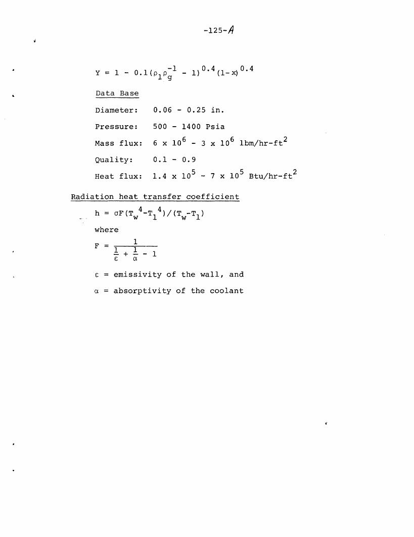
-125-4
Y = 1 - 0.1 (p g1O 1lPj9
Data Base
Diameter:
Pressure:
Mass flux:
Quality:
Heat flux:
- 1) ( 1-x)
0.06 - 0.25 in.
500 - 1400 Psia
6 x 106 x 106 lbm/hr-ft2
0.1 - 0.9
1.4 x 10⁵ - 7 x 10⁵ Btu/hr-ft2
Radiation heat transfer coefficient
h = oF(T 4 -T 14 )/(Tw-T1)
where
1 1+ 1 - 1
£ a
c = emissivity of the wall, and
a = absorptivity of the coolant

jl
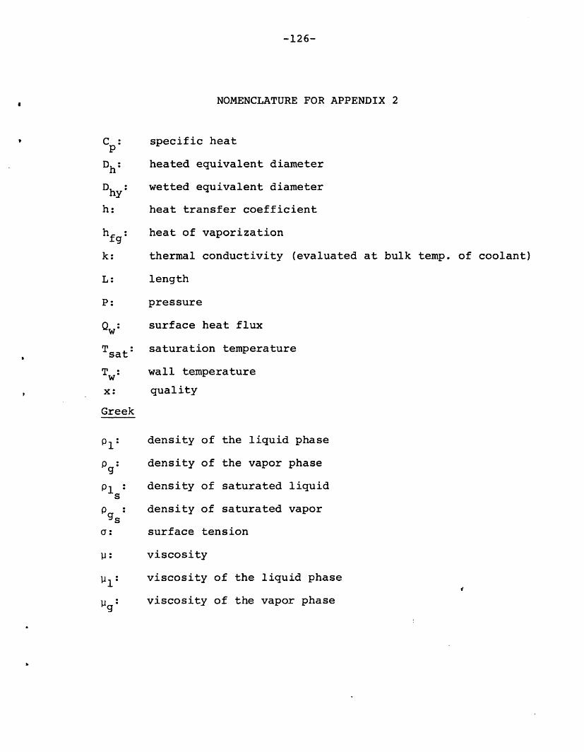
-126-
NOMENCLATURE FOR APPENDIX 2
C : specific heat
Dh: heated equivalent diameter
Dhy: wetted equivalent diameter
h: heat transfer coefficient
hfg: heat of vaporization
k: thermal conductivity (evaluated at bulk temp. of coolant)
L: length
P: pressure
QW surface heat flux
Tsat: saturation temperature
Tw: wall temperature
x: quality
Greek
pi: density of the liquid phase
Pg: density of the vapor phase
Pl ,: density of saturated liquid
p9 : density of saturated vaporgs
a: surface tension
P: viscosity
viscosity of the liquid phase
g19: viscosity of the vapor phase

-127-
Appendix 2 - References
A-1: F.W. Dittus and L.M.K. Boelter, "Heat Transfer inAutomobile Radiators of the Tubular Type," Universityof California Publications in Engineering, 2, 443-461,1930.
A-2: E.N. Seider and G.E. Tate, Ind. Eng. Chem., 28 (1936)412a-35.
A-3: J.R.S. Thom, W.M. Walker, T.A. Fallon and G.F.S. Reising,"Boiling in Subcooled Water During Flow Up Heated Tubesor Annuli," Proc. Instn. Mech. Engrs., 180 Pt 3c,226-246, 1966.
A-4: V.E. Schrock and L.M. Grossman, "Forced ConvectionVaporization Project," TID 14632, 1959.
A-5: J.C. Chen, "A correlation for boiling heat transfer tosaturated fluids in convective flow." Paper presentedto 6th National Heat Transfer Conference, Boston,11-14 Aug. 1963. ASME Preprint 63-HT-34.
A-6: J.S. Gellerstedt et al, "Two Phase Flow and HeatTransfer in Rod Bundles," ASME Conference, Los Angeles,California, Nov. 18, 1969.
A-7: L.S. Tong, Boiling Crisis and CriticalIHeat Flux,TID-25887 (1972).
A-8: P.G. Barnett, A Comparison of the Accuracy of SomeCorrelations for Burnout in Annuli and Rod Bundles,AEEW-R558 (1968).
A-9: L. Biasi et al, "Studies on Burnout," Part 3, EnergiaNuclear, 14, S (1967).
A-10: P. Griffith, T.C. Avedisian and J.P. Walkush, "Counter-current Flow Critical Heat Flux," Annual H.T. Conference,San Francisco, California, August 1975.
A-ll: J.B. McDonough, W. Milich, E.C. King, Partial FilmBoiling with Water at 2000 Psig in a Round VerticalTube, MSA Research Corp., Technical Report 62 (1958)(NP-6976).
A-12: Bjornard, T.A., "Blowdown Heat Transfer in A PressurizedWater Reactor," Ph.D. Thesis, M.I.T., August 1977.
-128-
A-13: R.S. Dougall and W.M. Rohsenow, Film Boiling on theInside of Vertical Tubes with Upward Flow of the Fluidat Low Qualities, MIT-TR-9079-26 (1963).
A-14: D.C. Groenveld, "Post-Dryout Heat Transfer at ReactorOperating Conditions," AECL-4513 (1973).

-129-
REPORTS IN REACTOR THERMAL HYDRAULICS RELATED TO THE
MIT ENERGY LABORATORY ELECTRIC POWER PROGRAM
A. Topical Reports (For availability check Energy LaboratoryHeadquarters, Room E19-439, MIT, Cambridge,Massachusetts, 02139)
A.1 General ApplicationsA.2 PWR ApplicationsA.3 BWR ApplicationsA.4 LMFBR Applications
A.1 M. Massoud, "A Condensed Review of Nuclear ReactorThermal-Hydraulic Computer Codes for Two-Phase FlowAnalysis", MIT Energy Laboratory Report MIT-EL-79-018,April 1979.
J.E. Kelly and M.S. Kazimi, "Development and Testingof the Three Dimensional, Two-Fluid Code THERMIT for LWRCore and Subchannel Applications", MIT Energy LaboratoryReport, MIT-EL-79-046, December 1979.
A.2 P. Moreno, C. Chiu, R. Bowring, E. Khan, J. Liu, N. Todreas,"Methods for Steady-State Thermal/Hydraulic Analysisof PWR Cores", Report MIT-EL-76-006, Rev. 1, July 1977(Orig. 3/77).
J.E. Kelly, J. Loomis, L. Wolf, "LWR Core Thermal-HydraulicAnalysis--Assessment and Comparison of the Range ofApplicability of the Codes COBRA IIIC/MIT and COBRA IV-1",Report MIT-EL-78-026, September 1978.
J. Liu, N. Todreas, "Transient Thermal Analysis of PWR'sby a Single Pass Procedure Using a Simplified Nodal Layout",Report MIT-EL-77-008, Final, February 1979, (Draft, June 1977).
J. Liu, N. Todreas, "The Comparison of Available Data onPWR Assembly Thermal Behavior with Analytic Predictions",Report MIT-EL-77-009, Final, February 1979, (Draft, June 1977).
-130-
A.3 L. Guillebaud, A. Levin, W. Boyd, A. Faya, L. Wolf, "WOSUB -A Subchannel Code for Steady-State and Transient Thermal-Hydraulic Analysis of Boiling Water Reactor Fuel Bundles",Vol. II, User's Manual, MIT-EL-78-024, July 1977.
L. Wolf, A. Faya, A. Levin, W. Boyd, L. Guillebaud, "WOSUBA Subchannel Code for Steady-State and Transient Thermal-Hydraulic Analysis of Boiling Water Reactor Fuel Pin Bundles",Vol. III, Assessment and Comparison, MIT-EL-78-025, October 1977.
L. Wolf, A. Faya, A. Levin, L. Guillebaud, "WOSUB - A SubchannelCode for Steady-State Reactor Fuel Pin Bundles", Vol. I, ModelDescription, MIT-EL-78-023, September 1978.
A. Faya, L. Wolf and N. Todreas, "Development of a Methodfor BWR Subchannel Analysis", MIT-EL 79-027, November 1979.
A. Faya, L. Wolf and N. Todreas, "CANAL User's Manual",MIT-EL 79-028, November 1979.
A.4 W.D. Hinkle, "Water Tests for Determining Post-VoidingBehavior in the LMFBR", MIT Energy Laboratory ReportMIT-EL-76-005, June 1976.
W.D. Hinkle, ed., "LMFBR Safety & Sodium Boiling - A Stateof the Art Report", Draft DOE Report, June 1978.
M.R. Granziera, P. Griffith, W.D. Hinkle, M.S. Kazimi, A. Levin,M. Manahan, A. Schor, N. Todreas, G. Wilson, "Developmentof Computer Code for Multi-dimensional Analysis of SodiumVoiding in the LMFBR", Preliminary Draft Report, July 1979.

-131-
B. Papers
B.1 General ApplicationsB.2 PWR ApplicationsB.3 BWR ApplicationsB.4 LMFBR Applications
B.1 J.E. Kelly and M.S. Kazimi, "Development of the Two-FluidMulti-Dimensional Code THERMIT for LWR Analysis", acceptedfor presentation 19th National Heat Transfer Conference,Orlando, Florida, August 1980.
B.2 P. Moreno, J. Liu, E. Khan and N. Todreas, "Steady-StateThermal Analysis of PWR's by a Simplified Method,"American Nuclear Society Transactions, Vol. 26, 1977, p. 465.
P. Moreno,J. Liu, E. Khan, N. Todreas, "Steady-StateThermal Analysis of PWR's by a Single Pass ProcedureUsing a Simplified Nodal Layout," Nuclear Engineeringand Design, Vol. 47, 1978, pp. 35-48.
C. Chiu, P. Moreno, R. Bowring, N. Todreas, "EnthalpyTransfer Between PWR Fuel Assemblies in Analysis by theLumped Subchannel Model," Nuclear Engineering and Design,Vol. 53, 1979, 165-186.
B. 3 L. Wolf and A. Faya, "A BWR Subchannel Code with DriftFlux and Vapor Diffusion Transport," American NuclearSociety Transactions, Vol. 28, 1978, p. 553.
B.4 W.D. Hinkle, (MIT), P.M. Tschamper (GE), M.H. Fontana,(ORNL), R.E. Henry, (ANL), and A. Padilla, (HEDL), forU.S. Department of Energy, "LMFBR Safety & Sodium Boiling,"paper presented at the ENS/ANS International TopicalMeeting on Nuclear Reactor Safety, October 16-19, 1978,Brussels, Belgium.
M.I. Autruffe, G.J. Wilson, B. Stewart and M.S. Kazimi,"A Proposed Momentum Exchange Coefficient for Two-PhaseModeling of Sodium Boiling", Proc. Int. Meeting Fast ReactorSafety Technology, Vol. 4, 2512-2521, Seatle, Washington,August, 1979.
M.R. Granziera and M.S. Kazimi, "NATOF-2D: A Two DimensionalTwo-Fluid Model for Sodium Flow Transient Analysis", Trans.ANS, 33, 515, November 1979.


![A Condensed Review of Nuclear Reactor Thermal - [email protected]](https://static.fdocuments.us/doc/165x107/620745aa49d709492c2fbd26/a-condensed-review-of-nuclear-reactor-thermal-emailprotected.jpg)