A conceptual framework for studying the strength of plant ... · REVIEW AND SYNTHESIS A conceptual...

REV IEW AND

SYNTHES IS A conceptual framework for studying the strength of plant–

animal mutualistic interactions

Diego P. V�azquez,1, 2* Rodrigo

Ramos-Jiliberto,3, 4 Pasquinell

Urbani,3 and Fernanda S.

Valdovinos5, 6

Abstract

The strength of species interactions influences strongly the structure and dynamics of ecologicalsystems. Thus, quantifying such strength is crucial to understand how species interactions shapecommunities and ecosystems. Although the concepts and measurement of interaction strength infood webs have received much attention, there has been comparatively little progress in the con-text of mutualism. We propose a conceptual scheme for studying the strength of plant–animalmutualistic interactions. We first review the interaction strength concepts developed for food webs,and explore how these concepts have been applied to mutualistic interactions. We then outlineand explain a conceptual framework for defining ecological effects in plant–animal mutualisms.We give recommendations for measuring interaction strength from data collected in field studiesbased on a proposed approach for the assessment of interaction strength in plant–animal mutual-isms. This approach is conceptually integrative and methodologically feasible, as it focuses on twokey variables usually measured in field studies: the frequency of interactions and the fitness com-ponents influenced by the interactions.

Keywords

Ecological networks, interaction strength, long-term effects, mutualism, plant–animal interactions,short-term effects.

Ecology Letters (2015) 18: 385–400

INTRODUCTION

Organisms interact with other organisms in multiple ways.The consequences of interactions for the participating speciesvary widely in their relative importance – from weak tostrong – and their sign – from negative to neutral to posi-tive. These features of species interactions influence stronglythe structure and dynamics of ecological systems (Yodzis1981; McCann et al. 1998; Wootton & Emmerson 2005;Bascompte et al. 2006; Okuyama & Holland 2008). Thus,quantifying the strength of the ecological interactions amongspecies and revealing their underlying mechanisms is crucialto understand how they contribute to shaping communitiesand ecosystems.Historically, ecological theory has focused mostly on antag-

onistic interactions, particularly predation and competition,and only in recent decades are mutualistic interactions beingincorporated into mainstream ecological theory (Bronstein1994; Stachowicz 2001; Bruno et al. 2003). The theoreticalconcepts and empirical measurement of the magnitude ofantagonistic interactions have received much attention (see,e.g. Paine 1992; Laska & Wooton 1998; Abrams 2001; Berlow

et al. 2004; Wootton & Emmerson 2005; Novak & Wootton2008), with substantial effort put into combining data andtheory (Laska & Wooton 1998; Wootton & Emmerson 2005).In contrast, there has been little discussion about the concep-tual basis of interaction strength in plant–animal mutualisms,in spite of the widespread occurrence of this type of mutual-ism in nature and its importance for the maintenance of natu-ral and agricultural ecosystems (Bronstein 1994; Stachowicz2001; Begon et al. 2006; Garibaldi et al. 2013). Furthermore,although several empirical studies have provided data on therelative importance of animal mutualists for particular plantspecies (Schemske & Horvitz 1984; Herrera 1987; Pettersson1991; Schupp 1993; Olsen 1997; V�azquez et al. 2005; Nesset al. 2006; Sahli & Conner 2006), little effort has been madeto estimate the reciprocal effects of plants on animals, and tolink theoretical concepts with data. Thus, there is a seriousvacuum in the development and application of ecological the-ory to the study of mutualism.Below we provide a synthesis of the concepts of interaction

strength developed in the context of antagonistic, consumer–resource interactions and apply them to the study of mutualisticinteractions.

1Instituto Argentino de Investigaciones de las Zonas �Aridas, CONICET, CC 507,

5500,Mendoza, Argentina2Facultad de Ciencias Exactas y Naturales, Universidad Nacional de Cuyo,

Centro Universitario, M5502JMA,Mendoza, Argentina3Centro Nacional del Medio Ambiente, Fundaci�on de la Universidad de Chile,

Av. Larra�ın 9975, La Reina, Santiago,Chile

4Instituto de Filosof�ıa y Ciencias de la Complejidad, Los Alerces 3024, ~Nu~noa,

Santiago,Chile5Department of Ecology and Evolutionary Biology, University of Arizona,

BSW 310, 1041 Lowell St., Tucson, AZ,85721,USA6Pacific Ecoinformatics and Computational Ecology Lab, 1604 McGee Avenue,

Berkeley, CA,94703,USA

*Correspondence: E-mail: [email protected]

© 2015 John Wiley & Sons Ltd/CNRS

Ecology Letters, (2015) 18: 385–400 doi: 10.1111/ele.12411

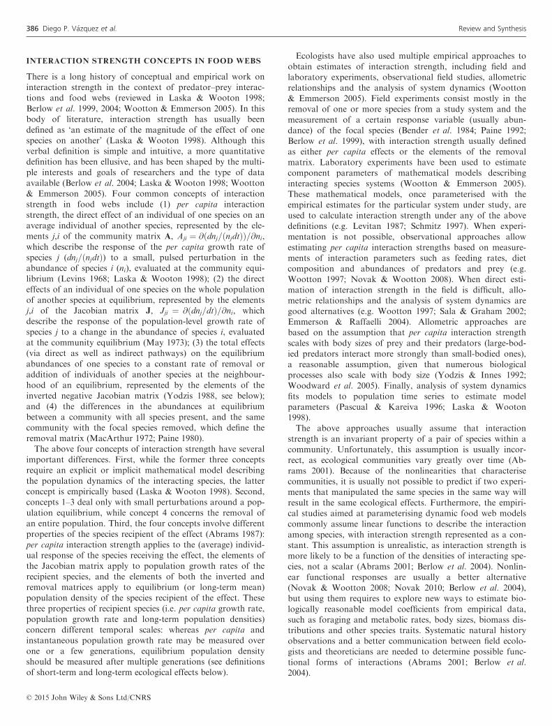
INTERACTION STRENGTH CONCEPTS IN FOOD WEBS

There is a long history of conceptual and empirical work oninteraction strength in the context of predator–prey interac-tions and food webs (reviewed in Laska & Wooton 1998;Berlow et al. 1999, 2004; Wootton & Emmerson 2005). In thisbody of literature, interaction strength has usually beendefined as ‘an estimate of the magnitude of the effect of onespecies on another’ (Laska & Wooton 1998). Although thisverbal definition is simple and intuitive, a more quantitativedefinition has been ellusive, and has been shaped by the multi-ple interests and goals of researchers and the type of dataavailable (Berlow et al. 2004; Laska & Wooton 1998; Wootton& Emmerson 2005). Four common concepts of interactionstrength in food webs include (1) per capita interactionstrength, the direct effect of an individual of one species on anaverage individual of another species, represented by the ele-ments j,i of the community matrix A, Aji ¼ @ðdnj=ðnjdtÞÞ=@ni,which describe the response of the per capita growth rate ofspecies j (dnj=ðnjdtÞ) to a small, pulsed perturbation in theabundance of species i (ni), evaluated at the community equi-librium (Levins 1968; Laska & Wooton 1998); (2) the directeffects of an individual of one species on the whole populationof another species at equilibrium, represented by the elementsj,i of the Jacobian matrix J, Jji ¼ @ðdnj=dtÞ=@ni, whichdescribe the response of the population-level growth rate ofspecies j to a change in the abundance of species i, evaluatedat the community equilibrium (May 1973); (3) the total effects(via direct as well as indirect pathways) on the equilibriumabundances of one species to a constant rate of removal oraddition of individuals of another species at the neighbour-hood of an equilibrium, represented by the elements of theinverted negative Jacobian matrix (Yodzis 1988, see below);and (4) the differences in the abundances at equilibriumbetween a community with all species present, and the samecommunity with the focal species removed, which define theremoval matrix (MacArthur 1972; Paine 1980).The above four concepts of interaction strength have several

important differences. First, while the former three conceptsrequire an explicit or implicit mathematical model describingthe population dynamics of the interacting species, the latterconcept is empirically based (Laska & Wooton 1998). Second,concepts 1–3 deal only with small perturbations around a pop-ulation equilibrium, while concept 4 concerns the removal ofan entire population. Third, the four concepts involve differentproperties of the species recipient of the effect (Abrams 1987):per capita interaction strength applies to the (average) individ-ual response of the species receiving the effect, the elements ofthe Jacobian matrix apply to population growth rates of therecipient species, and the elements of both the inverted andremoval matrices apply to equilibrium (or long-term mean)population density of the species recipient of the effect. Thesethree properties of recipient species (i.e. per capita growth rate,population growth rate and long-term population densities)concern different temporal scales: whereas per capita andinstantaneous population growth rate may be measured overone or a few generations, equilibrium population densityshould be measured after multiple generations (see definitionsof short-term and long-term ecological effects below).

Ecologists have also used multiple empirical approaches toobtain estimates of interaction strength, including field andlaboratory experiments, observational field studies, allometricrelationships and the analysis of system dynamics (Wootton& Emmerson 2005). Field experiments consist mostly in theremoval of one or more species from a study system and themeasurement of a certain response variable (usually abun-dance) of the focal species (Bender et al. 1984; Paine 1992;Berlow et al. 1999), with interaction strength usually definedas either per capita effects or the elements of the removalmatrix. Laboratory experiments have been used to estimatecomponent parameters of mathematical models describinginteracting species systems (Wootton & Emmerson 2005).These mathematical models, once parameterised with theempirical estimates for the particular system under study, areused to calculate interaction strength under any of the abovedefinitions (e.g. Levitan 1987; Schmitz 1997). When experi-mentation is not possible, observational approaches allowestimating per capita interaction strengths based on measure-ments of interaction parameters such as feeding rates, dietcomposition and abundances of predators and prey (e.g.Wootton 1997; Novak & Wootton 2008). When direct esti-mation of interaction strength in the field is difficult, allo-metric relationships and the analysis of system dynamics aregood alternatives (e.g. Wootton 1997; Sala & Graham 2002;Emmerson & Raffaelli 2004). Allometric approaches arebased on the assumption that per capita interaction strengthscales with body sizes of prey and their predators (large-bod-ied predators interact more strongly than small-bodied ones),a reasonable assumption, given that numerous biologicalprocesses also scale with body size (Yodzis & Innes 1992;Woodward et al. 2005). Finally, analysis of system dynamicsfits models to population time series to estimate modelparameters (Pascual & Kareiva 1996; Laska & Wooton1998).The above approaches usually assume that interaction

strength is an invariant property of a pair of species within acommunity. Unfortunately, this assumption is usually incor-rect, as ecological communities vary greatly over time (Ab-rams 2001). Because of the nonlinearities that characterisecommunities, it is usually not possible to predict if two experi-ments that manipulated the same species in the same way willresult in the same ecological effects. Furthermore, the empiri-cal studies aimed at parameterising dynamic food web modelscommonly assume linear functions to describe the interactionamong species, with interaction strength represented as a con-stant. This assumption is unrealistic, as interaction strength ismore likely to be a function of the densities of interacting spe-cies, not a scalar (Abrams 2001; Berlow et al. 2004). Nonlin-ear functional responses are usually a better alternative(Novak & Wootton 2008; Novak 2010; Berlow et al. 2004),but using them requires to explore new ways to estimate bio-logically reasonable model coefficients from empirical data,such as foraging and metabolic rates, body sizes, biomass dis-tributions and other species traits. Systematic natural historyobservations and a better communication between field ecolo-gists and theoreticians are needed to determine possible func-tional forms of interactions (Abrams 2001; Berlow et al.2004).


386 Diego P. V�azquez et al. Review and Synthesis

INTERACTION STRENGTH CONCEPTS APPLIED TO

PLANT–ANIMAL MUTUALISMS

As with the development of general ecological theory, thedevelopment of interaction strength concepts for mutualisticinteractions has lagged behind conceptual development forpredator–prey interactions. Box 1 presents the main classes ofmodels that have been used to study the population dynamicsof mutualistic interactions. As in food webs, the simplestmathematical models of mutualistic interactions have definedinteraction strength as a single parameter aij representing theper capita effect of an individual of species j on an individualof species i, assuming a linear (type I) functional response forthe mutualistic interaction (the third term of the equations forModel class 1 in Box 1). However, a type I functionalresponse is obviously unrealistic, as the benefit of a mutualis-tic interaction cannot increase indefinitely with increasingabundance of the interaction partner, unless we make theassumption of being at the close vicinity of an equilibrium.Other models use instead a saturating function to representthe mutualistic interaction (typically a type II functionalresponse; the third term in equations for Model class 2), thusassuming that the effect of an interaction saturates withincreasing abundance of all the interaction partners. In princi-ple, this function could also have a peak of the benefit atintermediate mutualist densities, beyond which the benefit ofthe interaction would decrease (Holland et al. 2002; Morriset al. 2010), thus approaching a type IV functional response(Andrews 1968). This class of models has also been mademore complex by incorporating interspecific competitionamong species of the same guild, i.e. among pollinator speciesand among plant species (Bastolla et al. 2009). A third classof models is based on the logistic equation, assuming that thecarrying capacity of each mutualist species depends on thedensity of its interaction partners. More mechanistically, con-sumer–resource models envision mutualistic interactions as aspecial case of consumer–resource dynamics, which considerthe transfer of energy and/or nutrients between an organism(consumer) and a resource (Holland et al. 2002; Holland &DeAngelis 2010). A fifth class of models incorporates adaptivebehaviour of pollinators and floral resources as a separatestate variable in consumer–resource mutualistic models (Vald-ovinos et al. 2013). These mechanistic consumer–resourcemodels include several key processes involved in these mutual-istic interactions, and are thus a promising approach to com-bine theory and data, and to synthesise mutualistic and foodweb theory. A final class of models considers a landscape ofpatches occupied by plants and animals interacting mutualisti-cally, in which the fraction of patches occupied by plants andanimals results from the balance between colonisation andextinction. The choice of the model of mutualistic interactionsis crucial for our understanding of the dynamics of mutualis-tic systems, because it may affect strongly the results and con-clusions of model-based assessments of interaction strength.Ecologists have not always been consistent in their defini-

tion of interaction strength in the above dynamic models ofmutualistic interactions. In the first two classes of models ofBox 1, interaction strength has usually been defined explicitlyas the per capita effect of one species on another (i.e. aij and

aji). Some other studies (Ramos-Jiliberto et al. 2009, 2012;Valdovinos et al. 2009, 2013) have used species removal tostudy the resulting community patterns and dynamics, whichis similar to the removal matrix approach described above forfood webs. In many other studies of plant–animal mutualisticnetworks, the underlying definition of interaction strength isstill less clear.Compared to predator–prey interactions, in the context of

mutualistic interactions there has been relatively little effort toquantify interaction strength empirically with measures thatare relevant at the level of demography and populationdynamics. Many studies of plant–animal mutualisms havedefined related concepts such as ‘effectiveness’ (Schupp 1993;Olsen 1997; V�azquez et al. 2005; Sahli & Conner 2006), ‘effi-ciency’ (Schemske & Horvitz 1984; Pettersson 1991) or ‘qual-ity’ (Herrera 1987; Ness et al. 2006). These concepts areusually defined as the contribution of an animal mutualist tothe reproduction of a plant. For example, Schupp (1993, p.16) defines the effectiveness of a seed disperser species on aplant species as ‘the number of new adults resulting from thedispersal activities of a disperser’ (see also Schupp et al.2010). Similarly, Herrera (1987) defines the ‘quality’ of an eco-logical interaction as ‘the fitness consequences of the interac-tion when it occurs’. In addition, some recent studies havealso performed manipulative removal experiments to assessthe short-term effect of animal (Brosi & Briggs 2013) or plant(Lopezaraiza-Mikel et al. 2007) species on other species of thecommunity. Brosi & Briggs (2013) conducted experimentalremovals of the most abundant pollinator species from severalstudy plots in sub-alpine meadows, recording the change inthe seed production of a focal plant species, which is close toestimating some elements of the removal matrix. Similarly,Lopezaraiza-Mikel et al. (2007) experimentally removed theflowers of the alien plant Impatiens glandulifera and exploredthe response of the rest of the assemblage of co-floweringnative plants in terms of flower visitation and pollen transportby pollinators. Most of these studies have considered only theplant’s perspective (i.e. the animal’s effect on the plant’s fit-ness), although recently some studies have started to consideralso the animal’s perspective (i.e. the plant’s effect on the ani-mal’s fitness; see, e.g. Roulston & Goodell 2011; V�azquezet al. 2012).Because quantifying interaction strength in the field is diffi-

cult and time-consuming, it may be unfeasible to obtain suchestimates for all pairwise interactions in a network. To cir-cumvent this problem, interaction frequency (e.g. the numberof visits of pollinators or frugivores to plants) has been sug-gested as a good proxy for the magnitude of effects betweenpairs of interacting species. Specifically, V�azquez et al. (2005)showed mathematically that interaction frequency will be agood proxy for total (population level) effects of animals onplants when the magnitude of variation in interaction fre-quency is large compared to the magnitude of variation in theper-visit effect, and/or when total effects and per-visit effectsare positively correlated. Analysis of empirical data of theeffects of pollinators or frugivores on plants, and of plants onpollinators, confirmed interaction frequency as a good surro-gate of the magnitude of interactions in several species(V�azquez et al. 2005, 2012). We come back to this issue below


Review and Synthesis Interaction strength in mutualistic interactions 387

Box 1 Representative classes of population dynamic models of mutualistic interactions

We have identified six major classes of population dynamic models of mutualistic interactions. In model classes 1–5 below, Pi

and Aj are the abundances of plant and animal species.

1. Classic Lotka–Volterra model with linear functional response for mutualistic interaction (Gause & Witt 1935; Vandermeer & Boucher

1978; Travis & Post 1979; Heithaus et al. 1980; Addicott 1981; Wolin & Lawlor 1984; Ringel et al. 1996; Bascompte et al. 2006):

dPi

dt¼ riPi � ciP

2i þ

Xmj¼1

aijPiAj

dAj

dt¼ rjAj � cjA

2j þ

Xni¼1

ajiPiAj

Here, the first term of both equations represents exponential growth governed by the intrinsic growth rates of plants (ri) andanimals (rj), the second term intraspecific competition governed by coefficients ci and cj, and the third term the mutualisticinteraction with a linear functional response, summed for all mutualist species interacting with a focal species, governed by percapita interaction strength coefficients aij and aji. In the sums, m and n are the total number of plant and animal species in thecommunity, respectively.

2. Lotka–Volterra model with saturating functional response for mutualistic interaction (Holland et al. 2002, 2006; Okuyama & Holland

2008; Bastolla et al. 2009):

dPi

dt¼ riPi �

Xmk¼1

cikPkPi þXnj¼1

aijPiAj

1þ aijhijAj

dAj

dt¼ rjAj �

Xnl¼1

cilAlAj þXmi¼1

ajiPiAj

1þ ajihjiPi

A key difference between this model class and the previous one is the form of the third term, which in this case is a saturatingfunctional response, governed by per capita interaction strengths aij and aji and by handling times hij and hji. In some versionsof this class of models (e.g. Holland et al. 2002, 2006; Okuyama & Holland 2008) the second term includes only intra-specificcompetition, as in model class 1 (i.e. ciP

2i and cjA

2j ), whereas more recent versions (e.g. Bastolla et al. 2009) include both intra-

and interspecific competition (i.e.Pm

k¼1 cikPkPi andPn

l¼1 cilAlAj).

3. Logistic model modified with carrying capacity as a function of density of interaction partners (Whittaker 1975; May, 1976, 1981;

Addicott 1981; Wolin & Lawlor 1984):

dPi

dt¼ riPi 1� PiPm

j¼1 fðAjÞ

!

dAj

dt¼ rjAj 1� AjPn

i¼1 gðPiÞ� �

This third class of models is based on the logistic equation, in which exponential growth (riPi and rjAj) is limited by density-dependent regulation, with the carrying capacity of each population defined as a function of the abundances of its interactionpartners (functions fðAjÞ and gðPiÞ).

4. Consumer–resource (Holland et al. 2002; Holland & DeAngelis 2010):

dP

dt¼ rpPþ cp

apaPAhpa þ A

� �� qp

bpPA

epa þ P

� �� dpP

dA

dt¼ raAþ ca

aapPAhap þ P

� �� qa

baPAeap þ A

� �� daA

In consumer–resource models, exponential growth (first term) is regulated by the benefits (second term) and costs (third term)of the interaction, resulting from the production of the resources by each interacting species, with constants cp, ca, qp and qarepresenting conversion rates, apa, aap, bpa and bap representing the saturation levels and hpa, hap, epa and eap representing the



(see Quantifying effect strength of plant–animal mutualisticinteractions in nature).Another approach to the assessment of interaction strength

in mutualistic interactions considers phenology as a strongdeterminant of the outcome of interactions. Encinas-Viso et al.(2012), in parallel and with similar arguments to Nakazawa &Doi (2012) for food webs, assumed that the temporal overlapbetween interacting species, resulting from their phenologicaldynamics, defines interaction strengths. The rationale is that,as species do not interact uninterruptedly through time inmany ecosystems, their interactions are annulled when theiractive stages (e.g. flowers and active pollinators) disappeartemporarily from the system. In addition, as the length of phe-nophases varies largely among species, it is likely that thelength of temporal overlap between phenophases of interactingspecies explains a large part of the variance in effect strength.

Under this view, instantaneous effect strength is less importantfor defining annual average effect strength. Remarkably, Enc-inas-Viso et al. (2012) found that phenology, without invokingother biological constraints, can largely explain the main topo-logical properties observed in real plant–animal mutualisticwebs, such as high nestedness and limited connectance. Inaddition, they found that the length of the season affectsstrongly the stability and diversity of mutualistic webs.From the preceding paragraphs it is evident that the use of

interaction strength concepts in the context of mutualisticinteractions has been conceptually and empirically limited,thus providing a motivation for further synthesis. In theremainder of the article, we outline a conceptual scheme fordefining effects in ecological interactions in general and inplant–animal mutualistic interactions in particular. This con-ceptual framework encompasses most previous concepts of

half saturation constants; the fourth term represents density-dependent mortality, governed by death rates dp and da. Note thatthis model has been proposed by Holland et al. (2002) and Holland & DeAngelis (2010) for two species P and A, and to ourknowledge it has not been extended to multispecies systems.

5. Consumer–resource with adaptive foraging and floral resources as state variables (Valdovinos et al. 2013):

dPi

dt¼ rið1�

Xl

clPlÞXj

eijrijVijðPi;Aj; aijÞ � diPi

dAj

dt¼Xi

cijfijðRi;PiÞVijðPi;Aj; aijÞ � djAj

dRi

dt¼ biPi � /iRi �

Xj

fijðRi;PiÞVijðPi;Aj; aijÞ

daijdt

¼ Gi

AjcijfijðRi;PiÞVijðPi;Aj; aijÞ � aij

Xmk¼1

ckjfkjðRk;PkÞVijðPi;Aj; aijÞ !

Here, plants exhibit intra and interspecific density-dependence of magnitude c in their recruitment rate, which is governed bythe rate Vij ¼ PiAjaijsij at which pollinators of each species visit the plant. The function aij is the foraging effort displayed bypollinator j on plant i, which takes values between 0 and 1; the sum of aij over all plants visited by pollinator j is equal to one.The parameter sij is the visitation efficiency of animal j to plant i. The parameter Gj is the basal adaptation rate of foraging aijof animal j on its plant resources, i.e. the speed of change in aij when the term within parenthesis in the equation for daij=dt isnon-zero. The parameter sij is the visitation efficiency of animal j to plant i. Animals grow by consumption rate fij of floralresources R in their visits to host plants. Floral resources R are produced at a rate b, self-limited at a rate / and consumed byanimal visitors. Parameters eij, rij and cij are conversion terms, while ri and di have the same meaning as in other model classes.

6. Patch dynamics (Armstrong 1987; Amarasekare 2004; Fortuna & Bascompte 2006; Ramos-Jiliberto et al. 2009, 2012; Valdovinos

et al. 2009):

dPi

dt¼Xnj¼1

cijPiAj

X

� �ð1� d� PiÞ � eiPi

dAj

dt¼ cjAjðX� AjÞ � ejAj

In this last class of models, Pi and Aj represent the fraction of patches occupied by plant and animal species i and j, modeled asfunctions of colonisation and extinction rates for plants (cij and ei) and animals (cj and ej), the fraction of patches lost by habi-tat destruction, and the total number of available patches for animals (Ω).

Box 1 Continued



interaction strength proposed in the literature. We illustratethis framework by applying it to a model community of inter-acting plants and pollinators, and give recommendations forits application to data collection in field studies.

A CONCEPTUAL FRAMEWORK FOR ECOLOGICAL

EFFECTS IN PLANT–ANIMAL MUTUALISTIC

INTERACTIONS

Any interaction between two species can be defined as thereciprocal influence that the species exert on each other. Aninteraction thus involves a bidirectional causal influence,which can be decomposed into its constituent unidirectionaleffects of each species on the other (Fig. 1). More precisely,an effect can be defined as the capacity to transmit changesbetween variables (species’ attributes in this case; Pearl 2009;ArunKumar & Venkatesan 2011). As it is unlikely that thetwo effects of a pair of interacting species have the same mag-nitude, the term ‘interaction strength’ commonly used in theecological literature is ambiguous, and it is thus more mean-ingful to refer instead to ‘effect strength’. Defining effects alsorequires specifying the relevant attributes whose change istransmitted from the emitter to the receptor of the effect –usually abundance (n) for the emitter and some property ofthe temporal trajectory of abundance (s) for the receptor. Inaddition, behaviour could also be used as a meaningful vari-able for both emitter and receptor. Thus, most commonly theecological effect of species i on species j represents how achange in the abundance of species i (ni) triggers a deviationin the abundance trajectory of species j (sj). While a change inabundance is an easily measurable property of ecological pop-ulations, a change in the trajectory of abundance is more elu-sive, and, as we will see below, depends on the temporal scaleat which interaction strength is defined.When dealing with ecological effects, it is important to

make a distinction between the different time frames in whichwe measure the response of one species to another. In theshort term, a change in the receptor species follows as animmediate response to the instantaneous change (usually interms of abundance) in the species exerting the effect (theemitter). In contrast, in the long term, a sustained change inthe emitter will cause a change in the focal (receptor) species,but also in other intermediate species acting as secondaryemitters. In addition, the altered focal receptor species willdrive further modifications in their neighbours that will betransmitted back to the focal receptor, and so on, until the

entire system reaches a new steady state. Long-term effectswill thus encompass the time needed to reach a new steadystate, which will depend on the dynamics of the system andthus on the generation times of the species involved (Yodzis1988). Therefore, as shown below, long-term effects can bereduced to a combination of short-term effects determined bythe structure of interactions in the community.The precise definitions of short-term and long-term effect

strength will depend on how we define the trajectory of thereceptor species j, sj. For short-term effects, it is customary todefine sj as dnj=ðnjdtÞ, the per capita rate of population change(Wootton & Emmerson 2005). Then,

Dji ¼ @

@ni

dnjnjdt

� �ð1Þ

where Dji is the strength of the short-term, per capita effectthat species i exerts on species j, which is equal to the ele-ments of the community matrix (Levins 1968).Long-term effects are a function of a specific set of direct

and indirect effects, i.e. the direct effects between the twofocal species and the other direct effects between all pairs ofinteracting species in their ‘sphere of influence’ (the state andfunctioning of all species directly or indirectly involved in theinteraction; Brose et al. 2005). Thus, for long-term effects, percapita rate of change is not the best measure of sj, because inthe long-term it approaches zero whenever a new equilibriumis reached, and thus the effect strength will be entirely deter-mined by the growth rate of the receptor (which could also bezero) at the instant of exerting a perturbation. Instead, long-term population density at equilibrium, n�j , is a more appro-priate measure of sj. Thus, we can define long-term effectstrength as Lji ¼ dn�j =dIi, where Ii is the rate of adding orremoving individuals of species i. As shown in detail byDambacher et al. (2005), the calculation of long-term effectstrength can be done by means of the inverse of the negativeJacobian matrix, J (see definition for J above, section Interac-tion strength concepts in food webs). Using the propertyM�1 ¼ adjðMÞ=detðMÞ, where M�1 is the inverse, adj(M) theadjugate, and det(M) the determinant of a matrix M (Damb-acher et al. 2005), we can express the magnitude of long-termeffects as

Lji ¼dn�jdIi

¼ 1

detð�JÞ adjð�JÞji ð2Þ

As long as we are interested in the relative strength ofeffects within a community, the first part of the rightmostexpression can be disregarded and we can redefine the long-term (net) effect of species i on species j as

Lji ¼ adjð�JÞji ð3ÞA property of eqn 3 is that it includes terms of the growth

equations of species other than i and j, which are not directlyinvolved in the focal interaction. Thus, in general Lji will be afunction of its sphere of influence. The subset of species deter-mining the effect strength in a focal interaction is defined by thefunctional relationships assumed for the population dynamics(‘dynamic rules’) and by the pattern of interactions among thespecies within the community (‘network topology’).

x1 x2

x1 x2

x1 x2

= +

Interaction

Effects

Figure 1 Ecological interactions and effects. For a given ecological

interaction between two species x1 and x2, there are two unidirectional

effects, one exerted by x1 on x2, and the reciprocal effect of x2 on x1.



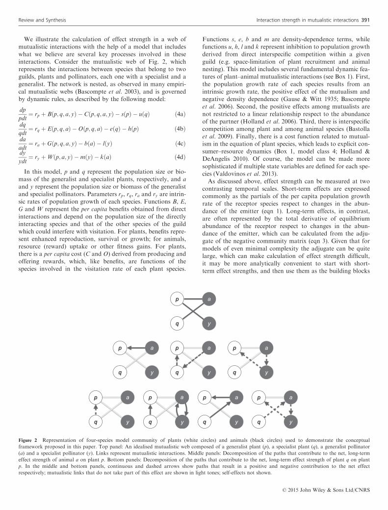
We illustrate the calculation of effect strength in a web ofmutualistic interactions with the help of a model that includeswhat we believe are several key processes involved in theseinteractions. Consider the mutualistic web of Fig. 2, whichrepresents the interactions between species that belong to twoguilds, plants and pollinators, each one with a specialist and ageneralist. The network is nested, as observed in many empiri-cal mutualistic webs (Bascompte et al. 2003), and is governedby dynamic rules, as described by the following model:

dp

pdt¼ rp þ Bðp; q; a; yÞ � Cðp; q; a; yÞ � sðpÞ � uðqÞ ð4aÞ

dq

qdt¼ rq þ Eðp; q; aÞ �Oðp; q; aÞ � eðqÞ � hðpÞ ð4bÞ

da

adt¼ ra þ Gðp; q; a; yÞ � bðaÞ � lðyÞ ð4cÞ

dy

ydt¼ ry þWðp; a; yÞ �mðyÞ � kðaÞ ð4dÞ

In this model, p and q represent the population size or bio-mass of the generalist and specialist plants, respectively, and aand y represent the population size or biomass of the generalistand specialist pollinators. Parameters rp, rq, ra and ry are intrin-sic rates of population growth of each species. Functions B, E,G and W represent the per capita benefits obtained from directinteractions and depend on the population size of the directlyinteracting species and that of the other species of the guildwhich could interfere with visitation. For plants, benefits repre-sent enhanced reproduction, survival or growth; for animals,resource (reward) uptake or other fitness gains. For plants,there is a per capita cost (C and O) derived from producing andoffering rewards, which, like benefits, are functions of thespecies involved in the visitation rate of each plant species.

Functions s, e, b and m are density-dependence terms, whilefunctions u, h, l and k represent inhibition to population growthderived from direct interspecific competition within a givenguild (e.g. space-limitation of plant recruitment and animalnesting). This model includes several fundamental dynamic fea-tures of plant–animal mutualistic interactions (see Box 1). First,the population growth rate of each species results from anintrinsic growth rate, the positive effect of the mutualism andnegative density dependence (Gause & Witt 1935; Bascompteet al. 2006). Second, the positive effects among mutualists arenot restricted to a linear relationship respect to the abundanceof the partner (Holland et al. 2006). Third, there is interspecificcompetition among plant and among animal species (Bastollaet al. 2009). Finally, there is a cost function related to mutual-ism in the equation of plant species, which leads to explicit con-sumer–resource dynamics (Box 1, model class 4; Holland &DeAngelis 2010). Of course, the model can be made moresophisticated if multiple state variables are defined for each spe-cies (Valdovinos et al. 2013).As discussed above, effect strength can be measured at two

contrasting temporal scales. Short-term effects are expressedcommonly as the partials of the per capita population growthrate of the receptor species respect to changes in the abun-dance of the emitter (eqn 1). Long-term effects, in contrast,are often represented by the total derivative of equilibriumabundance of the receptor respect to changes in the abun-dance of the emitter, which can be calculated from the adju-gate of the negative community matrix (eqn 3). Given that formodels of even minimal complexity the adjugate can be quitelarge, which can make calculation of effect strength difficult,it may be more analytically convenient to start with short-term effect strengths, and then use them as the building blocks

p a

q y

p a

yq

p a

yq

p a

yq

p a

q y

p a

q i

p a

q y

p a

q y

a

y

Figure 2 Representation of four-species model community of plants (white circles) and animals (black circles) used to demonstrate the conceptual

framework proposed in this paper. Top panel: An idealised mutualistic web composed of a generalist plant (p), a specialist plant (q), a generalist pollinator

(a) and a specialist pollinator (y). Links represent mutualistic interactions. Middle panels: Decomposition of the paths that contribute to the net, long-term

effect strength of animal a on plant p. Bottom panels: Decomposition of the paths that contribute to the net, long-term effect strength of plant q on plant

p. In the middle and bottom panels, continuous and dashed arrows show paths that result in a positive and negative contribution to the net effect

respectively; mutualistic links that do not take part of this effect are shown in light tones; self-effects not shown.



of long-term effects. For example, for the general model (eqn4), short-term effect strength of other species on the generalistplant p are

@

@q

dp

pdt¼ @Bðp; q; a; yÞ

@q� @uðqÞ

@qð5aÞ

@

@a

dp


@a� @Cðp; q; a; yÞ

@að5bÞ

@

@y

dp


@y� @Cðp; q; a; yÞ

@yð5cÞ

It should be noted that effect strength between species thatbelong to the same guild is given by the difference betweenthe gain in benefit as a consequence of the interaction and thefitness loss produced by the direct competition between theinteracting species. On the other hand, the effect strengthbetween species of different guilds is given by the differencebetween the gain in benefit as a consequence of the interactionand the fitness loss produced by the cost of the interaction.For simplicity, such cost is assumed to be null in the case ofanimals, although it may be included if needed.Long-term effect strength, measured through the elements

of the adjugate of the negative Jacobian matrix, gives thechange in equilibrium density of the receiver as a consequenceof a constant influx of individuals of the emitter species.Long-term effects are usually composed of many terms andthus they are difficult to measure in real communities. Belowwe present the effect strength between species of differentguilds and between species of the same guild in our study sys-tem (eqn 4). Specifically, we will consider the effects of an ani-mal on a plant, and between plants, by applying eqn 3 to theJacobian matrix associated to the system represented by eqn4. Thus, the long-term effect strength of the generalist animalon the generalist plant is

Lpa ¼ DyyðDpaDqq �DqaDpqÞ �DqqDyaDpy ð6Þwhere Dji refers to the short-term, direct effects of species i onspecies j, as given in eqn 1. Making certain reasonableassumptions, it is often possible to know the sign of eachdirect effect and that of each term in the right hand of eqn 6.For example, we assume that the direct benefit of a mutualis-tic interaction exceeds the cost associated to it, and that thedirect interactions between species of the same guild are nega-tive due to interference and competition. Notice that the spe-cific functional form of each Dji term in eqn 6 as well as thegeneral structure of Lpa will depend on the particular modelconsidered (see, e.g. Box 1), and the network structure of thesystem. It should also be noted that the net, long-term effectof a on p is composed of three feedback cycles, in this casethree paths (Fig. 2). The first path is the direct effect and con-tributes positively to the long-term effect. The second pathcontributes negatively to the total effect, and represents thebeneficial effect of animal a on p’s competitor q. This trans-lates into a negative indirect path from a to p. The last com-ponent of the long-term effect constitutes also a negativecontribution, and represents the suppression of animal y’sgrowth rate by its competitor, which leads to a reduced mutu-alistic effect of y on p.The long-term effect strength of the specialist plant on the

generalist plant is given by

Lpq ¼ DpqðDaaDyy �DayDyaÞ �DpaDaqDyy þDaqDyaDpy ð7ÞFour feedback cycles compose this net effect (Fig. 2, bottom

panel). The first cycle is governed by the direct, short-term neg-ative effect of q on p driven by direct competition. The secondcycle is a positive contribution to this long-term effect, whichresults from the negative of the product between two subcom-ponents: a positive feedback cycle (two mutually detrimentalshort-term effects due to competition) between the two animals,and a negative short-term effect of q on p. The third cycle is apositive contribution to the net effect, given by indirect mutual-ism from q to p through a. The last component is a negativecontribution (which reinforces the negative effect), governed bythe enhancement by q of the growth rate of a, which suppressesits competitor y, finally suppressing the growth rate of p.The above mathematical framework is consistent with the

interaction strength concepts most widely used in the ecologi-cal literature (Brose et al. 2004; Wootton & Emmerson 2005).Thus, given a proper model of community dynamics, thisframework allows us to define short-term and long-term effectstrength by eqns 1 and 3 respectively.

QUANTIFYING EFFECT STRENGTH OF PLANT–

ANIMAL MUTUALISTIC INTERACTIONS IN NATURE

Measuring effect strength in the field usually involves a greatexperimental effort, especially for assessing the magnitude oflong-term effects, Lji. There are two main ways of measuringLji: directly, or indirectly by combining a series of short-termeffects (Fig. 3). We can assess Lji directly through press per-turbation experiments, in which the perturbation is sustainedthrough an extended period of time (Bender et al. 1984). Adirect assessment of Lji through press experiments requiresmanipulating the population density (adding or, more simply,removing individuals) of the emitter in a sustained way, andrecording the change in equilibrium abundance in the receptorspecies by comparing the manipulated plots with appropriatecontrols. The time span needed for this kind of experiments isusually long.Alternatively, we can measure long-term effects indirectly

by measuring a series of short-term effects, which can be donethrough at least three alternative routes (Fig. 3). First, asmentioned above for food webs (see section Interactionstrength concepts in food webs), we can conduct field experi-ments and observations to parameterise a dynamic modelsuch as that presented in eqn 4, calculate the short-term asshown in eqn 5 and then use them to construct the Jacobianmatrix to calculate long-term effects (eqn 3), as illustrated ineqns 6 and 7. Although this approach may be feasible for sim-ple systems with few interacting species as in the above exam-ple (eqn 4), it may become logistically unfeasible for largersystems.A second route for calculating long-term effects indirectly

by combining a series of short-term effects is to conduct pulseexperiments, in which the perturbation occurs once at a spe-cific point in time (Bender et al. 1984; Paine 1992). As wehave seen above (eqns 6 and 7), each element of Lji is com-puted as a function of a specific set of elements Dkl. For



brevity, we define the per capita population growth rate asFk ¼ dnk=ðnkdtÞ, which can be inserted into eqn 1 to obtainDkl ¼ @Fk=@nl. The Dkl elements represent direct interactionsbetween species that belong to the sphere of influence of Lji.For simplicity, we define this set as Sji ¼ fDkl for all speciesk and l that belong to the sphere of influence of Ljig. Forcomputing a given Lji from its Dkl components it is necessaryto know the species composition and topology of the commu-nity. Then, from this information we obtain the communitystructure represented by the structure of the Jacobian matrixJ (see details in Box 2). Nevertheless, note that even so adynamic model is not necessary at this step, as the proceduresoutlined in Box 2 rest on a specific set of assumptions thatlead to the basic structure of effects among the species (i.e.which elements of the Jacobian matrix are zero and which arenot); this set of assumptions represents in fact a model. Byapplying eqn 3 to the J matrix we obtain the symbolic expres-sions for calculating long-term effects, including the set Sij.We can concentrate our experimental effort on measuringeach element Dkl. Thus, we can perform a pulse experimentfor each Dkl, after which the change in the per capita popula-tion growth rate of the receptor, relative to the control, isrecorded.Unfortunately, the use of pulse experiments, although stan-

dard in ecology for measuring short-term effects, is not a pan-acea. Short-term effects should be measured with this methodby introducing a constant flux of emitter individuals in thepopulation, which is impossible because organisms come inintegers, and then estimating the derivative of abundance withrespect to time at the moment of the introduction, which isalso often violated because some time after the pulsed intro-duction is needed for detecting changes in population sizes.To minimise these problems, experimenters should avoid con-ducting pulse experiments on small populations, and shouldrecord the response of the receiver species shortly after the

manipulation. Even more important, experimenters shouldbear in mind that the errors of these calculations will accumu-late when combining several Dkl estimates to calculate Lji.That said, Schmitz (1997) has shown that calculating long-term effects through the inverse Jacobian matrix (as shown ineqns 2, 3, 6 and 7) is a useful tool for assessing the qualitativeoutcome of long-term experiments, even under a considerableamount of variation in the values of the responses. Further-more, although conducting pulse experiments is certainly pos-sible (see, e.g. Lopezaraiza-Mikel et al. 2007; Brosi & Briggs2013), they still require substantial experimental effort, and inmany situations they may be unfeasible, especially for com-munity-wide studies involving many pairs of interacting plantand animal species.A third route to calculate long-term effects indirectly by

combining a series of short-term effects, which allow a furtherreduction in experimental effort, is to decompose each short-term effect Dkl into quantities that are easier to measure inthe field (Fig. 3). For simplicity, we start by assuming that theper capita rate of change of the receptor is determined entirely(or is extremely sensitive to) a given fitness component, suchas seed production, fecundity or survival. To this end, it ispossible to use the chain rule of differential calculus todecompose Dkl in terms of fitness components and the fre-quency of interaction events,

Dkl ¼ @Fk

@nl¼ @Fk

@Zk

@Zk

@Vkl

@Vkl

@nlð8Þ

where Fk is the per capita population growth rate of the recep-tor species k (as defined in eqn 1), Zk is a fitness componentof the receptor likely to respond to the interaction with theemitter species l, Vkl is the frequency of interaction eventsbetween species k and l, and nl is the abundance of the emitterspecies l (see Box 2 for the use of short-term effects to calcu-late long-term effects, and Box 3 for the derivation and

Field assessment of responses of

component(s) of the receptor

receptor to interaction frequency interaction frequency to abundance of the emitter

Pulse experiment Press experiment

Experimental assessment of

population parameters

Parameterization of a dynamic

model

Decomposition of short term effect

Short term effect Long term effect

Figure 3 Multiple approaches for estimating short- and long-term effects (filled boxes) in plant–animal mutualistic interactions. Boxes at the base of the

diagram indicate the basic empirical measures needed for the assessments. Long-term effects can be assessed directly through press experiments (sustained

alteration of the emitter’s abundance). Alternatively, long-term effects can be assessed indirectly from short-term effects through the experimental

assessment of parameters of dynamic population models, pulse experiments or the field assessment of components of short-term effects (see text for details).



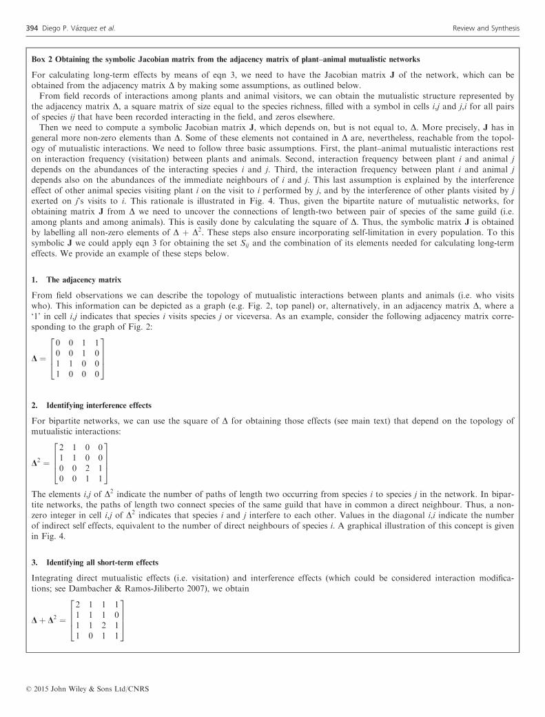
Box 2 Obtaining the symbolic Jacobian matrix from the adjacency matrix of plant–animal mutualistic networks

For calculating long-term effects by means of eqn 3, we need to have the Jacobian matrix J of the network, which can beobtained from the adjacency matrix D by making some assumptions, as outlined below.From field records of interactions among plants and animal visitors, we can obtain the mutualistic structure represented by

the adjacency matrix D, a square matrix of size equal to the species richness, filled with a symbol in cells i,j and j,i for all pairsof species ij that have been recorded interacting in the field, and zeros elsewhere.Then we need to compute a symbolic Jacobian matrix J, which depends on, but is not equal to, D. More precisely, J has in

general more non-zero elements than D. Some of these elements not contained in D are, nevertheless, reachable from the topol-ogy of mutualistic interactions. We need to follow three basic assumptions. First, the plant–animal mutualistic interactions reston interaction frequency (visitation) between plants and animals. Second, interaction frequency between plant i and animal jdepends on the abundances of the interacting species i and j. Third, the interaction frequency between plant i and animal jdepends also on the abundances of the immediate neighbours of i and j. This last assumption is explained by the interferenceeffect of other animal species visiting plant i on the visit to i performed by j, and by the interference of other plants visited by jexerted on j’s visits to i. This rationale is illustrated in Fig. 4. Thus, given the bipartite nature of mutualistic networks, forobtaining matrix J from D we need to uncover the connections of length-two between pair of species of the same guild (i.e.among plants and among animals). This is easily done by calculating the square of D. Thus, the symbolic matrix J is obtainedby labelling all non-zero elements of D þ D2. These steps also ensure incorporating self-limitation in every population. To thissymbolic J we could apply eqn 3 for obtaining the set Sij and the combination of its elements needed for calculating long-termeffects. We provide an example of these steps below.

1. The adjacency matrix

From field observations we can describe the topology of mutualistic interactions between plants and animals (i.e. who visitswho). This information can be depicted as a graph (e.g. Fig. 2, top panel) or, alternatively, in an adjacency matrix D, where a‘1’ in cell i,j indicates that species i visits species j or viceversa. As an example, consider the following adjacency matrix corre-sponding to the graph of Fig. 2:

D ¼0 0 1 10 0 1 01 1 0 01 0 0 0

2664

3775

2. Identifying interference effects

For bipartite networks, we can use the square of D for obtaining those effects (see main text) that depend on the topology ofmutualistic interactions:

D2 ¼2 1 0 01 1 0 00 0 2 10 0 1 1

2664

3775

The elements i,j of D2 indicate the number of paths of length two occurring from species i to species j in the network. In bipar-tite networks, the paths of length two connect species of the same guild that have in common a direct neighbour. Thus, a non-zero integer in cell i,j of D2 indicates that species i and j interfere to each other. Values in the diagonal i,i indicate the numberof indirect self effects, equivalent to the number of direct neighbours of species i. A graphical illustration of this concept is givenin Fig. 4.

3. Identifying all short-term effects

Integrating direct mutualistic effects (i.e. visitation) and interference effects (which could be considered interaction modifica-tions; see Dambacher & Ramos-Jiliberto 2007), we obtain

Dþ D2 ¼2 1 1 11 1 1 01 1 2 11 0 1 1

2664

3775



rationale behind eqn 8). Note that eqn 8 assumes for simplic-ity that the influence that the abundance of the emitter speciesnl exerts on the interaction frequency between the receptor kand its other neighbours (different from l) is negligible (seeBox 3). Given that these derivatives are functions that canhardly be assumed to be linear, in practice they must be eval-uated at a specific point within the variable’s space. This pointcould be, for example the set of abundances and traits presentat the instant of the investigation, or at a future time, whenthe community reaches equilibrium. Thus, the first (left) termof the rightmost expression of eqn 8 represents the effect thatthe change in a fitness component of species k exerts on itsown per capita growth rate, the second term is the effect thatthe change in the frequency of interaction events between spe-cies k and l exerts on the fitness component Zk, which cap-tures the positive and negative terms of eqn 5, and the thirdterm is the effect that the change in the abundance of species lexerts on the frequency of interaction events between speciesk and l. Incorporating frequency of interaction in the estima-tion of Dkl makes sense, given that in plant–animal mutual-

isms individuals are involved in multiple interaction eventsthroughout their lifespan (i.e. a bee visits many flowers), aproperty of plant–animal mutualistic interactions that setsthem apart from food webs. Note that, in the context of bene-fit–cost model discussed in the previous section (eqns 4 and5), the benefit–cost relationship is implicit in the short-termeffects described by eqn 8, as it represents the net benefits thatcan normally be observed in field studies (i.e. gross benefitsminus costs). As a whole, the three types of observationsinvolved in the decomposition of eqn 8 should be substan-tially simpler to obtain than manipulating the abundances ofeach emitter species and measuring the response in the recei-ver species in terms of its overall population growth rate.The choice of the fitness component Zk considered as surro-

gate of Fk is crucial for the assessment of effect strength. Twomain criteria should be borne in mind: the per capita rate ofchange of the receptor should be sensitive to the variation in thefitness component, and the fitness component should in turn besensitive to the variation in interaction frequency. The greaterthe product of these two sensitivities, the better the chosen fit-

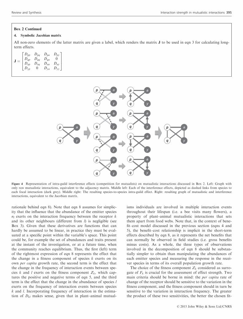
4. Symbolic Jacobian matrix

All non-zero elements of the latter matrix are given a label, which renders the matrix J to be used in eqn 3 for calculating long-term effects.

J ¼Dpp Dpq Dpa Dpy

Dqp Dqq Dqa 0Dap Daq Daa Day

Dyp 0 Dya Dyy

2664

3775

p a

q y

p a

q y

p a

q y

p a

q y

p a

q y

p a

q y

p a

q y

p a

q y

p a

q y

p a

q y

Figure 4 Representation of intra-guild interference effects (competition for mutualists) on mutualistic interactions discussed in Box 2. Left: Graph with

only raw mutualistic interactions, equivalent to the adjacency matrix. Middle left: Each of the interference effects, depicted as dashed links from species to

each focal interaction (dark grey). Middle right: The resulting species-to-species intra-guild effect. Right: resulting graph of mutualistic and interference

interactions, equivalent to the Jacobian matrix.

Box 2 Continued



ness component as a surrogate of Fk for the assessment of effectstrength. For example, for plant–pollinator interactions anobvious choice of a fitness component is seed production forplants, and either fecundity or survival for animals.In cases in which per capita population growth rate is not

uniquely determined by one fitness component involved in theplant–animal interaction under study, several components ofFk should be considered instead (Reed & Bryant 2004; Crone2001). In this case, it is also necessary to know the effect ofchanging the value of each chosen fitness component of thereceptor species on its own per capita growth rate. Thus, eachcomponent Dkl of the set Sji can be computed as

Dkl ¼ @Fk

@nl¼Xhr¼1

@Fk

@Zkr

@Zkr

@Vkl

@Vkl

@nlð9Þ

for any given set of h fitness components with valuesZk1;Zk2; . . .; Zkh.Once we have identified the appropriate fitness components

to be measured, we need to quantify the three partial deriva-tives in the rightmost expression of eqn 8 or 9. The first deriv-ative involves estimating the response of Fk to a particularfitness component Zk involved in the interaction (e.g. seedproduction), which is often done by constructing a matrixpopulation model and calculating sensitivities of the fitnesscomponents of interest (Caswell 2001). There are many goodexamples of this estimation (Bierzychudek 1982; Ehrl�en & Eri-ksson 1995; Parker 1997; Knight 2004; Ashman et al. 2004;Bruna et al. 2009; Law et al. 2010). Evaluating this first partof eqn 8 is important, as the fitness component affected bythe mutualistic interaction does not necessarily contribute sig-nificantly to population growth rate. For example, fecundityusually contributes poorly to growth rates of perennial plants(Bierzychudek 1982; Ehrl�en & Eriksson 1995; Parker 1997;Knight 2004; Feldman & Morris 2011).The next step in the decomposition of short-term effects is

to calculate the response of the fitness component Zk tochanges in the frequency of interaction events (the second par-tial derivative in the rightmost expression of eqns 8 and 9;Fig. 3). For example, for plants we can study the contributionof particular pollinator species to the seed production of aparticular plant species, which can be done with pollinatorexclusion experiments in which flowers are experimentallyexposed to one visit of a particular pollinator species and theresulting seed production is measured afterwards (e.g. Herrera1987; Olsen 1997; V�azquez et al. 2005; Sahli & Conner 2006);equivalent observations can be done for plant–seed disperserinteractions (e.g. Fleming & Williams 1990; Wheelwright1991; Jordano & Schupp 2000). For animals, we can studythe contribution of particular plant species to the reproduc-tion of a particular animal species (V�azquez et al. 2012).Finally, we must estimate the response of visitation fre-

quency to changes in the abundance of the emitter species(the rightmost partial derivative in eqn 8; Fig. 3). This can bedone easily in the field by counting the number of animal vis-its to plants (see, e.g. Herrera 1989; Fleming & Williams 1990;Olsen 1997; Jordano & Schupp 2000; V�azquez et al. 2005;Sahli & Conner 2006; V�azquez et al. 2012), weighing them bythe degree of daily, seasonal and interannual temporal overlap

between the interacting organisms, obtained from direct phe-nological observations (e.g. flowering, fruiting or nesting phe-nology). Thus, this term will be greater for species with longerdaily, seasonal and interannual overlap of their activity peri-ods. In addition, if among-species variation in the frequencyof interaction per emitter individual (third derivative) is sub-stantially greater than variation in the fitness response toincrements in visitation (the product of the first two deriva-tives), then the short-term effect strength could be approxi-mated using only information on the frequency of interactionevents (V�azquez et al. 2005, 2012). Note that the short-termeffect Dji as defined here is different from both interactionstrength (per visit) and species impact (per population) asdefined in V�azquez et al. (2012), but that it may be approxi-mated by species impact divided by abundances.

CONCLUDING REMARKS

We have outlined a conceptual framework that applies inter-action strength concepts to mutualistic interactions. Thisframework encompasses most definitions used in the food webliterature, and thus provides a conceptually solid basis forfuture discussions on the strength of plant–animal mutualisticinteractions.As is clear from our review, most past studies of plant–ani-

mal mutualistic interactions, included our own, have consid-ered interaction strength concepts implicitly and imprecisely.Furthermore, antagonistic (e.g. trophic) and mutualistic inter-actions differ in some obvious ways, which implies that inter-action strength concepts developed in the context ofantagonistic interactions cannot be automatically applied tomutualistic interactions. For example, whereas in predator–prey interactions prey are assumed to experience only detri-mental – either lethal or non-lethal – direct effects from theinteractions with their predator, in plant–animal mutualismsthe effects of interactions always have potential benefits andcosts. Another distinctive attribute of plant–animal mutual-isms is that all participant individuals are involved in multipleinteraction events throughout their lifespan, which again setsthem apart from food webs; visitation frequency is also ofparamount practical relevance, as it is this attribute of interac-tions what is usually recorded in field studies. For these rea-sons, improving the conceptual framework for defining andmeasuring interaction strength in plant–animal mutualisms isclearly necessary for further progress.Our framework emphasises the concept of unidirectional

effect as the basic component of ecological interactions.Although this concept is not new, we believe that applying itto the study of the strength of ecological interactions willhelp clarify its meaning, its quantitative definition and itsmeasurement. We have also emphasised the temporal scaleat which effect strength is defined, considering short-termeffects as the building blocks of long-term effects. Clearly,quantifying short-term effects will be considerably simplerand less prone to error than quantifying long-term effects.As we have proposed, such short-term effects can be esti-mated by considering key attributes of plant–animal mutual-istic interactions, namely the ability of plant and animalindividuals to interact multiple times throughout their



Box 3 Decomposition of short-term effects

In this box, we show the rationale and assumptions behind eqns 8–9 and their connection to the model proposed in eqn 4 andits derivatives in eqn 5. The discussion below applies to the effect strength of a generalist animal on a generalist plant (withpopulation sizes a and p respectively), as presented in our example if eqn 4 and Fig. 2. In this example, populations q and yrepresent, respectively, the population sizes of specialist plants and animals. Recall from eqn 4a the dynamics of the generalistplant:

dp

pdt¼ rp þ Bðp; q; a; yÞ � Cðp; q; a; yÞ � sp� uðqÞ ð10Þ

where the focal effect strength is defined in eqn 5b:

@

@a

dp


@a� @Cðp; q; a; yÞ

@a; ð11Þ

where, as defined in the main text, B and C are benefits and costs for the plant derived from the interaction with the animal.Here, it is assumed that the animal, through visiting the plant, modifies a plant’s fitness component (e.g. fertility) that increasesits per capita growth rate. At the same time, another plant’s fitness component (e.g. energy allocation to rewards) is promotedby the same animal that decreases the plant’s per capita rate of change.Assuming that the mutualist’s effects are mediated mainly by visitation rate Vpa of animals to plants and fitness component

Zp of the receptor species considered as a proper fitness proxy, we redefine the functions B and C (see also Box 2) as

Bðp; q; a; yÞ ¼ BðZp1ðVpaðp; q; a; yÞ;Vpyðp; a; yÞÞÞ ð12ÞCðp; q; a; yÞ ¼ CðZp2ðVpaðp; q; a; yÞ;Vpyðp; a; yÞÞÞ; ð13Þwhere Zp1 and Zp2 are two fitness components of the plant that determine benefits and costs for the plant, respectively, of itsmutualistic interactions, and that depend on visitation rates from the animal mutualists. Then, substituting eqns 12 and 13 intoeqn 11 renders

@

@a

dp

pdt¼ @

@aBðZp1ðVpaðp; q; a; yÞ;Vpyðp; a; yÞÞÞ � @

@aCðZp2ðVpaðp; q; a; yÞ;Vpyðp; a; yÞÞÞ: ð14Þ

Applying the chain rule and rearranging terms, the above expression expands to

@

@a

dp

pdt¼ @

@Zp1BðZp1ðVpaðp; q; a; yÞ;Vpyðp; a; yÞÞÞ @Zp1

@Vpa

@Vpa

@a

� @

@Zp1CðZp2ðVpaðp; q; a; yÞ;Vpyðp; a; yÞÞÞ @Zp1

@Vpa

@Vpa

@a

þ @


@Vpa

@Vpa

@a

� @


@Vpa

@Vpa

@a

þ @


@Vpy

@Vpy

@a

� @


@Vpy

@Vpy

@a

þ @


@Vpy

@Vpy

@a

� @


@Vpy

@Vpy

@a:

ð15Þ

For simplicity, we assume@Vpa

@a � @Vpy

@a and neglect the last four lines of eqn 15. Then, grouping terms and dropping the argu-ments of B y C for readability,

@

@a

dp

pdt¼ @ðB� CÞ

@Zp1

@Zp1

@Vpa

@Vpa

@aþ @ðB� CÞ

@Zp2

@Zp2

@Vpa

@Vpa

@a: ð16Þ

Given that all terms other than B and C in eqn 10 are independent from Zp1 and Zp2, we have that @ðB�CÞ@Zp1

¼ @@Zp1

dppdt ¼ @Fp

@Zp1,

and an analogous expression for the fitness component Zp2. Then, eqn 16 becomes



lifespan, the influence of biological rythms of interacting spe-cies that determine frequency of interaction, and fitness com-ponents relevant at the level of demography and populationdynamics. The relative importance of these components asdeterminants of effect strength in plant–animal mutualisticinteractions in ecological communities stands out as a keyavenue for future research. Furthermore, our frameworkcould also be extended to incorporate the spatial and tempo-ral variation in the strength of ecological effects as an inher-ent feature of ecological interactions, which would help dealwith the problem of variability in interaction strengthspointed out by Abrams (2001) for food webs.Ecological interactions are the threads that weave together

the fabric of life. The structure of this fabric is shaped by therelative strength of the effects among interacting species.Quantifying the importance of these effects and understandinghow they contribute to shaping communities and ecosystemsis thus at the heart of our quest to grasp how nature works,how our activities influence it and what we can do to curbthese effects. Our review was motivated by the need of clarify-ing the conceptual framework for defining, analysing andassessing effect strength in the context of plant–animal mutu-alisms. Although, as we argued above, this type of ecologicalinteractions have several unique features that justify develop-ing their own conceptual framework, a more ambitious goalwould be the development of a comprehensive and inclusiveframework for effect strength in all classes of ecologicalinteractions. Developing such a framework represents a chal-lenging next step for the advancement of ecological theory.

ACKNOWLEDGEMENTS

This research was partly funded by grants from FONCyT–ANPCyT (PICT-2010-2779) and CONICET (PIP-112-200801-02781) to DPV, FONDECYT (grant 1120958) to RR-J andCONICYT doctoral scholarships to FSV and PU. Eric Ber-low, Kristina Cockle, Nat Holland, Bel�en Maldonado, MarkNovak, Natalia Schroeder, Nydia Vitale and three anonymousreviewers made useful suggestions on the manuscript.

AUTHORSHIP

All authors contributed substantially to all stages of thisresearch.

REFERENCES

Abrams, P.A. (1987). On classifying interactions between populations.

Oecologia, 73, 272–281.Abrams, P.A. (2001). Describing and quantifying interspecific

interactions: a commentary on recent approaches. Oikos, 94, 209–218.Addicott, J.F. (1981). Stability properties of two-species models of

mutualism: simulation studies. Oecologia, 49, 42–49.Amarasekare, P. (2004). Spatial dynamics of mutualistic interactions. J.

Anim. Ecol., 73, 128–142.Andrews, J.F. (1968). A mathematical model for the continuous culture

of microorganisms utilizing inhibitory substrates. Biotechnol. Bioeng.,

10, 707–723.Armstrong, R.A. (1987). A patch model of mutualism. J. Theor. Biol.,

125, 243–246.ArunKumar, N. & Venkatesan, P. (2011). Recent advancement in causal

inference. Int. J. Pharm. Sci. Rev. Res., 2, 10–19.Ashman, T.L., Knight, T.M., Steets, J.A., Amarasekare, P., Burd, M.,

Campbell, D.R., Dudash, M.R., Johnston, M.O., Mazer, S.J., Mitchell,

R.J., Morgan, M.T. & Wilson, W.G. (2004). Pollen limitation of plant

reproduction: ecological and evolutionary causes and consequences.

Ecology, 85, 2408–2421.Bascompte, J., Jordano, P., Meli�an, C.J. & Olesen, J.M. (2003). The

nested assembly of plant-animal mutualistic networks. Proc. Natl.

Acad. Sci. USA, 100, 9383–9387.Bascompte, J., Jordano, P. & Olesen, J.M. (2006). Asymmetric

coevolutionary networks facilitate biodiversity maintenance. Science,

312, 431–433.Bastolla, U., Fortuna, M.A., Pascual-Garcia, A., Ferrera, A., Luque, B.

& Bascompte, J. (2009). The architecture of mutualistic networks

minimizes competition and increases biodiversity. Nature, 458, 1018–1020.

Begon, M., Townsend, C.R. & Harper, J.L. (2006). Ecology: From

Individuals to Ecosystems. Blackwell Publishing, Malden, MA, USA.

Bender, E.A., Case, T.J. & Gilpin, M.E. (1984). Perturbation experiments

in community ecology: theory and practice. Ecology, 65, 1–13.Berlow, E.L., Navarrete, S.A., Briggs, C.J., Power, M.E. & Menge, B.A.

(1999). Quantifying variation in the strengths of species interactions.

Ecology, 80, 2206–2224.Berlow, E.L., Neutel, A.-M., Cohen, J.E., de Ruiter, P.C., Ebenman, B.,

Emmerson, M., et al. (2004). Interaction strengths in food webs: issues

and opportunities. J. Anim. Ecol., 73, 585–598.Bierzychudek, P. (1982). The demography of jack-in-the-pulpit, a forest

perennial that changes sex. Ecol. Monogr., 52, 335–351.Bronstein, J.L. (1994). Our current understanding of mutualism. Q. Rev.

Biol., 69, 31–51.Brose, U., Berlow, E.L. & Martinez, N.D. (2005). Scaling up keystone effects

from simple to complex ecological networks. Ecol. Lett., 8, 1317–1325.Brose, U., Ostling, A., Harrison, K. & Martinez, N.D. (2004). Unified

spatial scaling of species and their trophic interactions. Nature, 428,

167–171.

@Fp

@a¼ @Fp

@Zp1

@Zp1

@Vpa

@Vpa

@aþ @Fp

@Zp2

@Zp2

@Vpa

@Vpa

@a; ð17Þ

which is equivalent to eqn 9 in the main text for the above two plant fitness components. Finally, by assuming that only a sin-gle fitness component Zp1 is relevant for determining capita growth rate of species p (as assumed in eqn 8), then eqn 17 reducesto

@Fp

@a¼ @Fp

@Zp1

@Zp1

@Vpa

@Vpa

@a; ð18Þ

thus recovering eqn 8 of the main text. In the case that a fitness component under consideration could participate in determin-ing both cost and benefit functions B and C, this development also holds without significant changes.

Box 3 Continued



Brosi, B.J. & Briggs, H.M. (2013). Single pollinator species losses reduce

floral fidelity and plant reproductive function. Proc. Natl. Acad. Sci.

USA, 110, 13044–13048.Bruna, E.M., Fiske, I.J. & Trager, M.D. (2009). Habitat fragmentation

and plant populations: is what we know demographically irrelevant? J.

Veg. Sci., 20, 569–576.Bruno, J.F., Stachowicz, J.J. & Bertness, M.D. (2003). Inclusion of

facilitation into ecological theory. Trends Ecol. Evol., 18, 119–125.Caswell, H. (2001). Matrix Population Models: Construction, Analysis, and

Interpretation. Sinauer Associates, Suntherland, MA.

Crone, E.E. (2001). Is survivorship a better fitness surrogate than

fecundity? Evolution, 55, 2611–2614.Dambacher, J.M., Levins, R. & Rossignol, P.A. (2005). Life expectancy

change in perturbed communities: derivation and qualitative analysis.

Math. Biosci., 197, 1–14.Dambacher, J.M. & Ramos-Jiliberto, R. (2007). Understanding and

predicting effects of modified interactions through a qualitative analysis

of community structure. Q. Rev. Biol., 82, 227–250.Ehrl�en, J. & Eriksson, O. (1995). Pollen limitation and population growth

in a herbaceous perennial legume. Ecology, 76, 652–656.Emmerson, M.C. & Raffaelli, D. (2004). Predator-prey body size,

interaction strength and the stability of a real food web. J. Anim. Ecol.,

73, 399–409.Encinas-Viso, F., Revilla, T.A. & Etienne, R.S. (2012). Phenology drives

mutualistic network structure and diversity. Ecol. Lett., 15, 198–208.Feldman, T.S. & Morris, W.F. (2011). Higher survival at low density

counteracts lower fecundity to obviate allee effects in a perennial plant.

Afr. J. Ecol., 99, 1162–1170.Fleming, T.H. & Williams, C.F. (1990). Phenology, seed dispersal, and

recruitment in cecropia peltata (moraceae) in costa rican tropical dry

forest. J. Trop. Ecol., 6, 163–178.Fortuna, M.A. & Bascompte, J. (2006). Habitat loss and the structure of

plant-animal mutualistic networks. Ecol. Lett., 9, 281–286.Garibaldi, L.A., Steffan-Dewenter, I., Winfree, R., Aizen, M.A.,

Bommarco, R., Cunningham, S.A., et al. (2013). Wild pollinators

enhance fruit set of crops regardless of honey bee abundance. Science,

339, 1608–1611.Gause, G.F. & Witt, A.A. (1935). Behavior of mixed populations and the

problem of natural selection. Am. Nat., 69, 596–609.Heithaus, E.R., Culver, D.C. & Beattie, A.J. (1980). Models of ant–plant

mutualisms. Am. Nat., 116, 347.

Herrera, C.M. (1987). Components of pollinator quality: comparative

analysis of a diverse insect assemblage. Oikos, 50, 79–90.Herrera, C.M. (1989). Pollinator abundance, morphology, and flower

visitation rate: analysis of the quantity component in a plant-pollinator

system. Oecologia, 80, 241–248.Holland, J.N. & DeAngelis, D.L. (2010). A consumer–resource approach

to the density-dependent population dynamics of mutualism. Ecology,

91, 1286–1295.Holland, J.N., DeAngelis, D.L. & Bronstein, J.L. (2002). Population

dynamics and mutualism: functional responses of benefits and costs.

Am. Nat., 159, 231–244.Holland, J.N., Okuyama, T. & DeAngelis, D.L. (2006). Comment on

‘asymmetric coevolutionary networks facilitate biodiversity

maintenance’. Science, 313, 1887.

Jordano, P. & Schupp, E.W. (2000). Seed disperser effectiveness: the

quantity component and patterns of seed rain for prunus mahaleb.

Ecol. Monogr., 70, 591–615.Knight, T.M. (2004). The effects of herbivory and pollen limitation on a

declining population of trillium grandiflorum. Ecol. Appl., 14,

915–928.Laska, M.S. & Wooton, J.T. (1998). Theoretical concepts and empirical

approaches to measuring interaction strength. Ecology, 79, 461–476.Law, W., Salick, J. & Knight, T.M. (2010). The effects of pollen

limitation on population dynamics of snow lotus (Saussurea medusa

and S. laniceps, asteraceae): Threatened Tibetan medicinal plants of the

eastern Himalayas. Plant Ecol., 201, 343–357.

Levins, R. (1968). Evolution in Changing Environments. Princeton

University Press, Princeton, NJ.

Levitan, C. (1987). Formal stability analysis of a planktonic freshwater

community. In: Predation: Direct and Indirect Impacts on Aquatic

Communities (eds Kerfoot, W.C. & Sih, A.). University Press of New

England, Hanover, pp. 71–100.Lopezaraiza-Mikel, M., Hayes, R., Whalley, M. & Memmott, J. (2007).

The impact of an alien plant on a native plant-pollinator network: an

experimental approach. Ecol. Lett., 10, 539–550.MacArthur, R.H. (1972). Geographical Ecology. Princeton University

Press, Princeton, NJ.

May, R.M. (1973). Stability and Complexity in Model Ecosystems, 1st

edn. Princeton University Press, Princeton, NJ.

May, R.M. (1976). Mathematical aspects of the dynamics of animal

populations. In: Studies in Mathematical Biology (ed. Levin, S.A.).

American Mathematical Society, Providence, pp. 317–366.May, R.M. (1981). Models for two interacting populations. In:

Theoretical Ecology: Principles and Applications (ed. May, R.M.).

Blackwell Scientific, Oxford, UK, pp. 49–70.McCann, K., Hastings, A. & Huxel, G.R. (1998). Weak trophic

interactions and the balance of nature. Nature, 395, 794–797.Morris, W.F., V�azquez, D.P. & Chacoff, N.P. (2010). Benefit and cost

curves for typical pollination mutualisms. Ecology, 91, 1276–1285.Nakazawa, T. & Doi, H. (2012). A perspective on match/mismatch of

phenology in community contexts. Oikos, 121, 489–495.Ness, J.H., Morris, W.F. & Bronstein, J.L. (2006). Integrating quality and

quantity of mutualistic service to contrast ant species protecting

Ferocactus wislizeni. Ecology, 87, 912–921.Novak, M. (2010). Estimating interaction strengths in nature: experimental

support for an observational approach. Ecology, 91, 2394–2405.Novak, M. & Wootton, J. (2008). Estimating nonlinear interaction

strengths: an observation-based method for species-rich food webs.

Ecology, 89, 2083–2089.Okuyama, T. & Holland, J.N. (2008). Network structural properties

mediate the stability of mutualistic communities. Ecol. Lett., 11, 208–216.Olsen, K.M. (1997). Pollination effectiveness and pollinator importance in

a population of heterotheca subaxillaris (asteraceae). Oecologia, 109,

114–121.Paine, R.T. (1980). Food webs: linkage, interaction strength and

community infrastructure. J. Anim. Ecol., 49, 667–685.Paine, R.T. (1992). Food-web analysis through field measurement of per

capita interaction strength. Nature, 355, 73–75.Parker, I.M. (1997). Pollinator limitation of Cytisus scoparius (scotch

broom), an invasive exotic shrub. Ecology, 78, 1457–1470.Pascual, M.A. & Kareiva, P. (1996). Predicting the outcome of

competition using experimental data: maximum likelihood and bayesian

approaches. Ecology, 77, 337–349.Pearl, J. (2009). Causal inference in statistics: an overview. Stat. Surv., 3,

96–146.Pettersson, M.W. (1991). Pollination by a guild of fluctuating moth

populations: option for unspecialization in silence vulgaris. Afr. J.

Ecol., 79, 591–604.Ramos-Jiliberto, R., Albornoz, A.A., Valdovinos, F.S., Smith-Ram�ırez,

C., Arim, M., Armesto, J.J., et al. (2009). A network analysis of plant–pollinator interactions in temperate rain forests of chilo�e island, chile.

Oecologia, 160, 697–706.Ramos-Jiliberto, R., Valdovinos, F.S., Moisset de Espan�es, P. & Flores,

J.D. (2012). Topological plasticity incaeses robustness of mutualistic

networks. J. Anim. Ecol., 81, 896–904.Reed, D.H. & Bryant, E.H. (2004). Phenotypic correlations among fitness

and its components in a population of the housefly. J. Evol. Biol., 17,

919–923.Ringel, M.S., Hu, H.H. & Anderson, G. (1996). The stability and

persistence of mutualisms embedded in community interactions. Theor.

Popul. Biol., 50, 281–297.Roulston, T.H. & Goodell, K. (2011). The role of resources and risks in

regulating wild bee populations. Annu. Rev. Entomol., 56, 293–312.



Sahli, H. & Conner, J. (2006). Characterizing ecological generalization in

plant–pollination systems. Oecologia, 148, 365–372.Sala, E. & Graham, M.H. (2002). Community-wide distribution of

predator-prey interaction strength in kelp forests. Proc. Natl. Acad. Sci.

USA, 99, 3678–3683.Schemske, D.W. & Horvitz, C.C. (1984). Variation among floral visitors

in pollination ability: a precondition for mutualism specialization.

Science, 225, 519–521.Schmitz, O.J. (1997). Press perturbations and the predictability of

ecological interactions in a food web. Ecology, 78, 55–69.Schupp, E.W. (1993). Quantity, quality, and the effectiveness of seed

dispersal by animals. In: Frugivory and Seed Dispersal: Ecological and

Evolutionary Aspects (eds Fleming, T.H. & Estrada, A.). Kluwer

Academic Publishers, Dordrecht, 15–29.Schupp, E.W., Jordano, P. & G�omez, J.M. (2010). Seed dispersal

effectiveness revisited: a conceptual review. New Phytol., 188, 333–353.Stachowicz, J.J. (2001). Mutualism, facilitation, and the structure of

ecological communities. Bioscience, 51, 235–246.Travis, C.C. & Post, W.M. (1979). Dynamics and comparative statics of

mutualistic communities. J. Theor. Biol., 78, 553–571.Valdovinos, F.S., Moisset de Espan�es, P., Flores, J.D. & Ramos-Jiliberto,

R. (2013). Adaptive foraging allows the maintenance of biodiversity of

pollination networks. Oikos, 122, 907–917.Valdovinos, F.S., Ramos-Jiliberto, R., Flores, J.D., Espinoza, C. &

L�opez, G. (2009). Structure and dynamics of pollination networks: the

role of alien plants. Oikos, 118, 1190–1200.Vandermeer, J.H. & Boucher, D.H. (1978). Varieties of mutualistic

interactions in population models. J. Theor. Biol., 74, 549–558.V�azquez, D.P., Lom�ascolo, S.B., Maldonado, M.B., Chacoff, N.P.,

Dorado, J., Stevani, E.L., et al. (2012). The strength of plant–pollinatorinteractions. Ecology, 93, 719–725.

V�azquez, D.P., Morris, W.F. & Jordano, P. (2005). Interaction frequency

as a surrogate for the total effect of animal mutualists on plants. Ecol.

Lett., 8, 1088–1094.Wheelwright, N.T. (1991). How long do fruit-eating birds stay in the

plants where they feed. Biotropica, 23, 29–40.Whittaker, R.H. (1975). Communities and Ecosystems. MacMillan, New

York.

Wolin, C.L. & Lawlor, L.R. (1984). Models of facultative mutualism:

density effects. Am. Nat., 124, 843–862.Woodward, G., Ebenman, B., Emmerson, M., Montoya, J., Olesen, J.,

Valido, A., et al. (2005). Body size in ecological networks. Trends Ecol.

Evol., 20, 402–409.Wootton, J.T. (1997). Estimates and tests of per capita interaction

strength: diet, abundance, and impact of intertidally foraging birds.

Ecol. Monogr., 67, 45–64.Wootton, J.T. & Emmerson, M. (2005). Measurement of interaction

strength in nature. Annu. Rev. Ecol. Evol. Syst., 36, 419–444.Yodzis, P. (1981). The stability of real ecosystems. Nature, 289, 674–676.Yodzis, P. (1988). The indeterminacy of ecological interactions as

perceived through perturbation experiments. Ecology, 69, 508–515.Yodzis, P. & Innes, S. (1992). Body size and consumer-resource dynamics.

Am. Nat., 139, 1151–1175.

Editor, Micky EubanksManuscript received 4 August 2014First decision made 3 September 2014Second decision made 9 December 2014Manuscript accepted 4 January 2015



A conceptual framework for studying the strength of plant ... · REVIEW AND SYNTHESIS A conceptual...

Documents

Transcript of A conceptual framework for studying the strength of plant ... · REVIEW AND SYNTHESIS A conceptual...