A Conceptual Framework for Predictability Studies
23
OCTOBER 1999 3133 SCHNEIDER AND GRIFFIES q 1999 American Meteorological Society A Conceptual Framework for Predictability Studies TAPIO SCHNEIDER Atmospheric and Oceanic Sciences Program, Princeton University, Princeton, New Jersey STEPHEN M. GRIFFIES NOAA/Geophysical Fluid Dynamics Laboratory, Princeton, New Jersey (Manuscript received 24 September 1998, in final form 19 January 1999) ABSTRACT A conceptual framework is presented for a unified treatment of issues arising in a variety of predictability studies. The predictive power (PP), a predictability measure based on information–theoretical principles, lies at the center of this framework. The PP is invariant under linear coordinate transformations and applies to mul- tivariate predictions irrespective of assumptions about the probability distribution of prediction errors. For univariate Gaussian predictions, the PP reduces to conventional predictability measures that are based upon the ratio of the rms error of a model prediction over the rms error of the climatological mean prediction. Since climatic variability on intraseasonal to interdecadal timescales follows an approximately Gaussian distribution, the emphasis of this paper is on multivariate Gaussian random variables. Predictable and unpre- dictable components of multivariate Gaussian systems can be distinguished by predictable component analysis, a procedure derived from discriminant analysis: seeking components with large PP leads to an eigenvalue problem, whose solution yields uncorrelated components that are ordered by PP from largest to smallest. In a discussion of the application of the PP and the predictable component analysis in different types of predictability studies, studies are considered that use either ensemble integrations of numerical models or au- toregressive models fitted to observed or simulated data. An investigation of simulated multidecadal variability of the North Atlantic illustrates the proposed meth- odology. Reanalyzing an ensemble of integrations of the Geophysical Fluid Dynamics Laboratory coupled general circulation model confirms and refines earlier findings. With an autoregressive model fitted to a single integration of the same model, it is demonstrated that similar conclusions can be reached without resorting to computationally costly ensemble integrations. 1. Introduction Since Lorenz (1963) realized that chaotic dynamics may set bounds on the predictability of weather and climate, assessing the predictability of various processes in the atmosphere–ocean system has been the objective of numerous studies. These studies are of two kinds (Lorenz 1975). Predictability studies of the first kind address how the uncertainties in an initial state of the climate system affect the prediction of a later state. Ini- tial uncertainties amplify as the prediction lead time increases, thus limiting predictability of the first kind. For example, in weather forecasting, the uncertainty in the predicted state reaches, at a lead time of a few weeks, the climatological uncertainty, the uncertainty as to which atmospheric state may be realized when only the climatological mean is available as a prediction. Day- Corresponding author address: Tapio Schneider, AOS Program, Princeton University, Princeton, NJ 08544-0710. E-mail: [email protected] to-day weather variations are not predictable beyond this lead time. Predictability studies of the second kind address the predictability of the response of the climate system to changes in boundary conditions. The fact that the state of the climate system is not completely determined by the boundary conditions limits predictability of the sec- ond kind. For example, the internal variability of the atmosphere renders a multitude of atmospheric states consistent with a configuration of sea surface temper- atures (SSTs). It is uncertain which atmospheric state will be realized at a given time, even if the SST con- figuration at that time is known. A deviation of the SST from its climatological mean results in a predictable atmospheric response only if it reduces the uncertainty as to which atmospheric state may be realized to less than the climatological uncertainty. These two types of predictability studies have a num- ber of common features. Each, of course, requires a model that provides predictions of the process under consideration. Hence, predictability is always to be un- derstood as predictability within a given model frame-
Transcript of A Conceptual Framework for Predictability Studies
OCTOBER 1999 3133S C H N E I D E R A N D G R I F F I E S
q 1999 American Meteorological Society
A Conceptual Framework for Predictability Studies
TAPIO SCHNEIDER
Atmospheric and Oceanic Sciences Program, Princeton University, Princeton, New Jersey
STEPHEN M. GRIFFIES
NOAA/Geophysical Fluid Dynamics Laboratory, Princeton, New Jersey
(Manuscript received 24 September 1998, in final form 19 January 1999)
ABSTRACT
A conceptual framework is presented for a unified treatment of issues arising in a variety of predictabilitystudies. The predictive power (PP), a predictability measure based on information–theoretical principles, lies atthe center of this framework. The PP is invariant under linear coordinate transformations and applies to mul-tivariate predictions irrespective of assumptions about the probability distribution of prediction errors. Forunivariate Gaussian predictions, the PP reduces to conventional predictability measures that are based upon theratio of the rms error of a model prediction over the rms error of the climatological mean prediction.
Since climatic variability on intraseasonal to interdecadal timescales follows an approximately Gaussiandistribution, the emphasis of this paper is on multivariate Gaussian random variables. Predictable and unpre-dictable components of multivariate Gaussian systems can be distinguished by predictable component analysis,a procedure derived from discriminant analysis: seeking components with large PP leads to an eigenvalue problem,whose solution yields uncorrelated components that are ordered by PP from largest to smallest.
In a discussion of the application of the PP and the predictable component analysis in different types ofpredictability studies, studies are considered that use either ensemble integrations of numerical models or au-toregressive models fitted to observed or simulated data.
An investigation of simulated multidecadal variability of the North Atlantic illustrates the proposed meth-odology. Reanalyzing an ensemble of integrations of the Geophysical Fluid Dynamics Laboratory coupled generalcirculation model confirms and refines earlier findings. With an autoregressive model fitted to a single integrationof the same model, it is demonstrated that similar conclusions can be reached without resorting to computationallycostly ensemble integrations.
1. Introduction
Since Lorenz (1963) realized that chaotic dynamicsmay set bounds on the predictability of weather andclimate, assessing the predictability of various processesin the atmosphere–ocean system has been the objectiveof numerous studies. These studies are of two kinds(Lorenz 1975). Predictability studies of the first kindaddress how the uncertainties in an initial state of theclimate system affect the prediction of a later state. Ini-tial uncertainties amplify as the prediction lead timeincreases, thus limiting predictability of the first kind.For example, in weather forecasting, the uncertainty inthe predicted state reaches, at a lead time of a few weeks,the climatological uncertainty, the uncertainty as towhich atmospheric state may be realized when only theclimatological mean is available as a prediction. Day-
Corresponding author address: Tapio Schneider, AOS Program,Princeton University, Princeton, NJ 08544-0710.E-mail: [email protected]
to-day weather variations are not predictable beyond thislead time.
Predictability studies of the second kind address thepredictability of the response of the climate system tochanges in boundary conditions. The fact that the stateof the climate system is not completely determined bythe boundary conditions limits predictability of the sec-ond kind. For example, the internal variability of theatmosphere renders a multitude of atmospheric statesconsistent with a configuration of sea surface temper-atures (SSTs). It is uncertain which atmospheric statewill be realized at a given time, even if the SST con-figuration at that time is known. A deviation of the SSTfrom its climatological mean results in a predictableatmospheric response only if it reduces the uncertaintyas to which atmospheric state may be realized to lessthan the climatological uncertainty.
These two types of predictability studies have a num-ber of common features. Each, of course, requires amodel that provides predictions of the process underconsideration. Hence, predictability is always to be un-derstood as predictability within a given model frame-
3134 VOLUME 12J O U R N A L O F C L I M A T E
work. Each type of study also requires a quantitativemeasure of predictability. Suggestions for such mea-sures abound. Shukla (1981, 1985), Hayashi (1986),Murphy (1988), and Griffies and Bryan (1997b), forexample, offer quantitative definitions of the term pre-dictability itself, and Stern and Miyakoda (1995) definethe concept of reproducibility. All of the above mea-sures are based, in one way or another, on comparingthe root-mean-square (rms) error of a univariate modelprediction with the rms error of the prediction that con-sists of the climatological mean. The examined processis considered predictable if the rms error of the modelprediction is significantly smaller than the rms error ofthe climatological mean prediction. Such predictabilitymeasures have made possible the definition of local pre-dictability indexes and the study of regional variationsin the predictability of geophysical fields [see Shukla(1985) for a review].
Difficulties arise, however, when one tries to gener-alize these predictability measures for univariate vari-ables to the multivariate case, as one does, for example,when interested not in estimating the predictability ofa single scalar variable grid point by grid point, but inestimating the overall predictability of several geo-physical fields in some larger region. The initializationof ensemble integrations for numerical weather predic-tions (see, e.g., Palmer 1996, Palmer et al. 1998, andreferences therein) is an example of an inherently mul-tivariate problem. Difficulties for multivariate predic-tions arise because the rms prediction error depends onthe basis in which the fields are represented. This meansthat, although there is not always a natural choice of ametric to measure the prediction error, the outcome ofthe analysis depends on which metric is chosen.
Another shortcoming of error-based predictability in-dexes is that they assume the error distributions to beapproximately Gaussian. This may be too restrictive anassumption in many cases. The potential predictive util-ity of Anderson and Stern (1996) partially overcomesthis drawback of more traditional predictability mea-sures. Anderson and Stern do not merely compare therms error of a model-derived prediction with that of theclimatological mean prediction—that is, the standarddeviations of the corresponding error distributions—butthey compare the entire error distributions, without mak-ing assumptions about their shape. If the error distri-butions differ significantly, potential predictive utilityexists; otherwise, it does not. However, in contrast tothe ratio of the rms errors, for example, the potentialpredictive utility does not give a measure of a predic-tion’s ‘‘degree of uncertainty’’ but only makes state-ments about whether or not a given model prediction isbetter than the climatological mean prediction.
In addition to these drawbacks, many predictabilitymeasures have been defined only for specific study de-signs. Even in recent studies, authors have found it nec-essary to introduce predictability measures of their own.This circumstance highlights the lack of an overarching
conceptual framework that is sufficiently general to en-compass currently used study designs. Still, whether oneexamines predictability of the first kind or predictabilityof the second kind, whether one employs comprehensivegeneral circulation models (GCMs) to generate ensem-ble integrations or simpler empirical models fitted toobservations—all predictability studies have some es-sential features in common.
Focusing on the fundamental structure that all pre-dictability studies share, we will here develop a unifiedconceptual framework. In section 2, we first reduce thestochastic problems arising in predictability studies totheir basic structure by stripping them of application-specific details; at the same time, we introduce the ter-minology and notation used throughout the remainderof this paper. In this general context, we then turn toaddress issues that frequently arise in predictability stud-ies.
The key constituent of the methodology to be pre-sented is a predictability index that uses concepts frominformation theory to measure the uncertainty of a pre-diction. [Shannon and Weaver (1949), Brillouin (1956),and Papoulis (1991, chapter 15) provide surveys on in-formation theory.] The information–theoretical predict-ability index, the predictive power (PP), is defined insection 3. The PP applies to univariate as well as tomultivariate predictions. In contrast to measures basedon rms errors, the PP is invariant under arbitrary linearcoordinate transformations; thus, the difficulties arisingfrom the arbitrariness of an error metric are circum-vented. Moreover, in its most general form, the PP doesnot rely on specific assumptions about either the dis-tributions of the random variables involved or the mod-eling framework. In the special case of univariate andnormally distributed predictions, the PP reduces to theratio of the rms prediction error over the rms error ofthe climatological mean prediction (or, according to ourconventions, to one minus this ratio). The PP can there-fore be understood as a generalization of the above-cited predictability indexes.
Since empirical evidence (e.g., Toth 1991) suggeststhat aggregated climatic variables, such as space or timeaverages of geophysical fields, follow an approximatelyGaussian distribution, the bulk of this paper focuses onmultivariate Gaussian random variables. For Gaussiansystems, questions such as, ‘‘what are the most pre-dictable features of the system?’’ can be answered in asystematic manner. When the PP is used as the measureof predictive information in multivariate predictions,then the most predictable linear combination of statespace variables, or the most predictable component, isthe one that maximizes the PP. In section 4, we adapta procedure from discriminant analysis (see, e.g.,McLachlan 1992) to extract predictable components ofa system: seeking components with large PP leads toan eigenvalue problem, whose solution yields uncor-related components that are ordered by PP from largestto smallest. This way of extracting a system’s predict-

OCTOBER 1999 3135S C H N E I D E R A N D G R I F F I E S
able components, the predictable component analysis,is then compared with principal component analysis andwith recently proposed approaches for determining pre-dictable components (e.g., Hasselmann 1993).
Sections 5 and 6 give details for the application ofthe general methodology to specific types of predict-ability studies. Section 5 deals with studies that useensemble integrations to estimate predictability; pre-dictability studies of both the first and the second kindare considered. Section 6 discusses how autoregressivemodels, a paradigmatic class of empirical models, canbe employed to assess the predictability of processes inthe climate system.
In section 7, we illustrate the PP concept and thepredictable component analysis by investigating the pre-dictability of multidecadal North Atlantic variability(Halliwell 1997, 1998; Griffies and Bryan 1997a,b).Two approaches are taken; first, ensemble integrationsof a coupled atmosphere–ocean GCM, as performed byGriffies and Bryan (1997b), are reanalyzed with the newmethods; this will confirm and refine the earlier findingsof Griffies and Bryan. Second, it will be demonstratedthat with an autoregressive model fitted to a single in-tegration of the same GCM, similar conclusions can bereached without performing computationally costly en-semble integrations.
In section 8, we summarize our conclusions and com-ment on their relevance for future research. The appen-dix contains computational details of procedures laidout in the body of this paper.
2. The basic structure of predictability studies
Suppose the state of a time-evolving system at timeinstant n is represented by an m-dimensional state vectorXn. Since we are concerned with the evolution of dis-tributions of states, rather than the evolution of a singlestate, we take a stochastic perspective on the dynamicsof the system: the state is viewed as a random vectorand as such is characterized by a probability distributionfunction whose domain is the state space, the set of allvalues the state vector can possibly attain. Given, forexample, the time evolution of a geophysical field, thestate space may be the m-dimensional vector space ofa representation of the field by m linearly independentgrid point values or spectral coefficients. The probabilitydistribution associated with the state Xn is the clima-tological distribution of the geophysical field and re-flects the uncertainty in the system’s state when the cli-matological mean is the only available predictive in-formation. In this stochastic framework, a particular ob-servation xn is called a realization of the random statevector Xn. (To avoid ambiguities, we make the distinc-tion between a random variable and one of its realiza-tions explicit by using capital letters for the randomvariable and lowercase for the realization.)
Consider now the prediction of the state xn. An in-dividual prediction xn is usually a function of the states
at previous instants n 2 1, n 2 2, etc. The predictionmight, for example, be obtained as the mean of an en-semble of GCM integrations. In predictability studiesof the first kind, each member of the ensemble corre-sponds to a different initial condition drawn from aninitial state whose probability distribution reflects ob-servational uncertainties. In predictability studies of thesecond kind, the ensemble members form a sample ofthe distribution of those states that are consistent witha given boundary condition—with a particular config-uration of SST, for example. As an alternative to en-semble integrations, the prediction may be based on anempirical model fitted to observed or simulated data.
The index n labels the time for which a prediction ismade. In predictability studies of the first kind, the indexn designates the forecast lead time. Since the climato-logical distribution associated with the state Xn does notvary much over typical forecast lead times, it is usuallyassumed to be stationary and hence independent of n.In predictability studies of the second kind, the indexn usually designates the time of year for which a pre-diction is made—a particular season, for example—andthe climatological distribution associated with the stateXn depends on n. We will discuss the analysis of aprediction for a single instant n, but to make the de-pendence on the prediction time explicit, we still indexprediction-time dependent variables by n.
Because of the system’s stochastic nature, the pre-diction xn does not necessarily coincide with the actualrealization xn but is afflicted with a random predictionerror en [ xn 2 xn. The probability distribution of thecorresponding random variable En reflects the uncer-tainty that remains in the state after a prediction hasbecome available. If the prediction is obtained as themean of an ensemble, the differences between the in-dividual ensemble members and their mean form a sam-ple of the prediction error distribution. If the predictionis obtained from an empirical model, the distribution ofprediction errors must be derived from the assumptionsintrinsic to the empirical modeling framework.
Since the prediction error en is the difference betweenthe actually realized state xn and the prediction xn therealization xn of the system’s state can be written as thesum xn 5 xn 1 en. Expressed in terms of the corre-sponding random variables, this statement reads
Xn 5 Xn 1 En,
where the predictor Xn is the random function of whichthe prediction xn is a realization. Fundamental to thefollowing line of reasoning is the interpretation of theassociated probability distributions: the distribution ofthe state Xn is the climatological distribution, whichreflects the prior uncertainty as to which state may berealized before any predictive information besides theclimatological mean is available; the distribution of theprediction error En reflects the posterior uncertainty thatremains in the state after a prediction has become avail-able.
3136 VOLUME 12J O U R N A L O F C L I M A T E
Here we are exclusively concerned with how the ran-dom nature of the prediction error affects the predict-ability of state vector realizations. We assume that theprediction error has no systematic component, whichwould show as a nonzero error mean; that is, we assumethat the predictor is unbiased.1 The condition of unbi-asedness is automatically satisfied if the prediction isobtained as the mean of an ensemble (see section 5).Note, however, that unbiasedness in our context doesnot necessarily mean that the model provides unbiasedpredictions of the actual empirical system being mod-eled; we stay exclusively within the framework set bythe model that provides the predictions and merely re-quire that, within this framework, the prediction errorhave zero mean.
Within the given modeling framework, we now askthe questions, how much information about state real-izations does the predictor provide? and, if the systemhas any predictable components, which of those are themost predictable? More precisely, we want an appro-priate measure of predictability and a decomposition ofthe state space into subspaces that are ordered from mostpredictable to least predictable.
3. The predictive power
a. Derivation of the general form
If no more specific prediction for xn is available thanthe climatological mean, then the uncertainty in the sys-tem’s state is the climatological or prior uncertainty as-sociated with the climatological probability density thatcharacterizes the state vector Xn. The effect of the pre-dictor is to provide predictive information on the sys-tem’s state, thus reducing the state’s prior uncertaintyto the posterior uncertainty that remains after a specificprediction has become available. A state is not pre-dictable when its posterior uncertainty is as large as itsprior uncertainty—that is, when the prediction does notcontain predictive information in excess of the clima-tological mean—and its predictability increases with in-creasing predictive information.
Rendering this intuitive notion of predictability quan-titative requires a precise definition of the degree ofuncertainty associated with the probability density pX(x)of a random variable X. Such a definition, which is atthe heart of information theory (Brillouin 1956; Shan-non and Weaver 1949), was introduced by Shannon(1948), who showed that the entropy
S [ 2k dx p (x) log p (x) (1)X E X X
1 The assumption that the prediction error has no systematic com-ponent does not imply a ‘‘perfect model’’ assumption. Sections 6 and8 contain examples of how the proposed framework applies to ‘‘non-perfect model’’ contexts, namely, to modeling with autoregressivemodels and to the performance evaluation of forecasting models.
is a natural measure of the uncertainty associated witha random variable X. (The quantity SX is sometimescalled the information of the random variable X, mean-ing that on average the additional information SX isneeded to specify completely a realization of X.) Shan-non derived the entropy functional from a set of heuristicrequirements that any measure of uncertainty shouldfulfill and showed that the entropy is, up to the constantfactor k, the unique measure fulfilling these require-ments. The value of the constant k determines the unitsin which the entropy is measured. For thermodynamicsystems, k is Boltzmann’s constant. For discrete randomvariables, the integration in (1) must be replaced by asum, and k 5 1/log 2 is chosen so that the entropy SX
becomes the expected number of binary digits, or bits,needed to specify a particular realization of X. We setk 5 1/m, where m is the dimension of the state space,so that SX becomes the mean entropy per state vectorcomponent. Defining the entropy relative to the statespace dimension makes it possible to compare the en-tropies of random vectors of different dimensions.
Assuming state space vectors to be determined onlyup to some fixed accuracy allows one to think of thestate space as discrete. The prior entropy is then theSXn
average number of state vector bits that are undeter-mined when only the climatological mean is known.Similarly, the posterior entropy , the conditional en-SEn
tropy of the state given a prediction, is the averagenumber of state vector bits that remain undeterminedafter a prediction has become available. The differencebetween these entropies is the predictive information
Rn [ 2 ,S SX En n(2)
the average information about the state contained in aprediction. For a discrete system, the predictive infor-mation is the average number of state vector bits thata prediction determines.2
The predictive power is defined as
an [ 1 2 .2Rne (3)
Since no predictor should increase the uncertainty in astate to above the prior uncertainty, implying $SXn
, the predictive information Rn is a positive semi-SEn
definite quantity. Hence, the PP exhibits proper limitingbehavior: it is an index 0 # an # 1 that is zero if thepredictive information vanishes and that monotonicallyincreases with increasing predictive information, even-tually approaching unity in the limit of infinite predic-tive information.
The PP can be interpreted geometrically. If, as is com-mon practice, the entropy SX is evaluated with k 5 1in definition (1), then the exponential exp SX is the state
2 Readers familiar with information theory will recognize the closeanalogy between the predictive information and the rate of trans-mission in a noisy channel as considered by Shannon (1948). Theposterior entropy corresponds to Shannon’s equivocation.SEn

OCTOBER 1999 3137S C H N E I D E R A N D G R I F F I E S
space volume enclosing ‘‘reasonably probable’’ or ‘‘typ-ical’’ realizations of the random vector X (Shannon andWeaver 1949, p. 59; Papoulis 1991). We evaluate theentropy SX with k 5 1/m and call the exponential exp SX
the typical range. The typical range is the mth root ofthe volume of typical realizations and measures the meansize of the set of values typically taken by a randomvector component. Thus, the term exp(2Rn) 5 /exp SEn
in the predictive power (3) is a ratio of typicalexp SXn
ranges: it is the ‘‘typical range of a state vector componentgiven a prediction’’ over the ‘‘typical range of a clima-tological state vector component.’’ That is to say, theterm exp(2Rn) is the fraction of the climatological typicalrange that lies within a prediction’s ‘‘range of uncer-tainty.’’ The complement 1 2 exp(2Rn), the PP, is thetypical range fraction that the predictor eliminates fromthe climatological typical range. Therefore, the PP in-dicates the efficacy of the predictor in narrowing thetypical range of a state vector component.
Besides exhibiting proper limiting behavior and hav-ing an intuitive interpretation, any adequate predict-ability index should also be independent of the basis inwhich state vectors are represented. If, for example, thestate is a compound of several geophysical fields, itspredictability index should not depend on the units inwhich these fields are measured. Changing the dimen-sional scaling of some components of a state vectoramounts to transforming state space vectors x to therescaled vectors x9 by multiplication with a diagonalmatrix. Such a transformation should leave a predict-ability measure unchanged. More generally, we requirethe predictability measure to be invariant under linearcoordinate transformations that transform state spacevectors x to x9 5 Ux with arbitrary nonsingular matricesU. To check if the PP is invariant under such transfor-mations, note that the probability density functions pX
in the original coordinates and pX9 in the transformedcoordinates are related by pX(x) dx 5 pX9(x9) dx9, fromwhich it follows that pX(x) 5 |detU| pX9(x9). Using theserelations, one finds that the entropy (1) of the trans-formed variable X9 compared to that of the originalvariable X is changed only by the additive constantklog|detU|, which involves the determinant detU of thetransformation matrix U (Shannon and Weaver 1949, p.59). In the predictive information—the difference (2)between the prior and the posterior entropies—the con-stant terms klog|detU| cancel. Thus, the PP is indeedinvariant under arbitrary linear transformations of statespace coordinates.
The PP hence has desirable properties and is definedunder general circumstances; neither assumptions aboutthe modeling framework nor assumptions about the di-mension or distributions of the relevant random vari-ables were needed for the derivation. For univariate andpossibly for low-dimensional state vectors, the entropycan be estimated using standard procedures, which in-volve estimation of the probability density (see, e.g.,Silverman 1986; Scott 1992) and of the entropy as a
functional thereof (see, e.g., Prakasa Rao 1983; Dmi-triev and Tarasenko 1973; Ahmad and Lin 1976; Joe1989; Hall and Morton 1993). Thus, it may be possibleto obtain a predictability measure for, say, local precip-itation, a field for which neither the climatological dis-tribution nor the prediction error distribution is Gaussianand for which a predictability index based on rms errorsmay be inappropriate.
Whereas the PP in its most general form is applicableto low-dimensional predictions, for high-dimensionalstates estimation of the entropy from (1) may not befeasible when the available dataset is small. Our em-phasis, however, is on intraseasonal to interannual cli-mate predictability, as opposed to the predictability ofshorter-term weather processes. That the former kind ofvariability follows an approximately Gaussian distri-bution (see, e.g., Toth 1991) considerably simplifies thediscussion.
b. Simplifications for Gaussian random variables
For an m-dimensional Gaussian random vector X, theprobability density takes the form
2m /2 T(2p) 121p (x) 5 exp 2 x 2 ^X& S x 2 ^X& ,1 2 1 2X 1/2 [ ](detS) 2
where ^X& is the mean of X, the superscript ( · )T indicatesthe transpose of ( · ), and S21 is the inverse of the non-singular covariance matrix S. The entropy integral (1)of the Gaussian density pX is readily carried out andyields the entropy
kS 5 (m 1 m log 2p 1 logdet S) (4)X 2
as a function of the covariance matrix determinant. De-noting the covariance matrix of the state, the climato-logical covariance matrix, by
Sn 5 Cov(Xn)
and the covariance matrix of the prediction error by
Cn 5 Cov(En),
one finds from (2) the predictive information
k detCnR 5 2 log .n 1 22 detSn
Using the product theorem for determinants and sub-stituting k 5 1/m leads to the PP
an 5 1 2 (detGn)1/(2m), (5)
where
Gn [ Cn21Sn (6)
is called the predictive information matrix. The predic-tive information matrix is well-defined, provided thatthe climatological covariance matrix Sn is positive def-

3138 VOLUME 12J O U R N A L O F C L I M A T E
inite so that its inverse exists and is likewise symmetricand positive definite. Positive definiteness of the cli-matological covariance matrix is assumed in the fol-lowing theoretical developments. The complicationsarising in practice from singular covariance matrix es-timates will be dealt with in section 4c.
The interpretation of the PP as a ratio of typical rangescan now be made more concrete. From the entropy (4)of an m-dimensional Gaussian random vector X withcovariance matrix S follows, again taking k 5 1/m, thetypical range,
exp SX 5 2pe (detS)1/(2m) .Ï (7)
For a univariate random variable with m 5 1, the co-variance matrix S is a scalar variance, and the squareroot of this variance is the standard deviation s. There-fore, the typical range of a univariate Gaussian randomvariable, exp SX 5 2pes ø 4.13s, is proportional toÏthe standard deviation. For an m-dimensional Gaussianrandom vector X, the ellipsoid Ep(X) that is centeredon the mean of X and encloses some fraction 0 , p ,1 of the cumulative probability distribution has a volumeproportional to (detS)1/2 (Anderson 1984, 263). Sincethe volume of an ellipsoid is proportional to the productof the lengths of its semiaxes, the factor (detS)1/(2m) inthe typical range (7) is proportional to the geometricmean of the semiaxis lengths of the ellipsoid Ep(X).Hence, the term (detGn)1/(2m) 5 (detCn)1/(2m)(detSn)21/(2m)
in the PP is the ratio of the geometric mean of thesemiaxis lengths of the prediction error ellipsoid Ep(En)over the geometric mean of the semiaxis lengths of theclimatological ellipsoid Ep(Xn). This interpretation ofthe PP as a ratio of geometric means of semiaxis lengthsspecializes the above general interpretation of the PP toGaussian random variables.
For univariate state vectors, the covariance matricesin (6) are scalar variances; the predictive informationmatrix is the ratio of these variances; and the squareroot of these variances, the standard deviations, are therms errors. Therefore, the predictive power (5) reducesto one minus the ratio of the rms error of a predictionover the rms error of the climatological mean prediction.Similar predictability measures have been employed byseveral authors, for example, Hayashi (1986), Murphy(1988), and Stern and Miyakoda (1995). Thus, the PPcan be understood as a generalization of the univariateerror-ratio predictability measures to multivariate stateswith arbitrary probability distributions.
When the distribution of states is multivariate Gauss-ian, one might think that arguments based on a com-parison of prediction errors also lead to an adequatepredictability measure. The mean-squared prediction er-ror corresponds to the sum of the diagonal elements, orthe trace trCn, of the prediction error covariance matrixCn. Analogously, the trace trSn of the climatologicalcovariance matrix Sn gives the mean-squared error ofthe climatological mean prediction. Taking one minus
the ratio of the rms errors as a predictability index, oneobtains
1/2trCn1 2 . (8)1 2trSn
Traces, however, are only invariant under orthogonaltransformations, a subclass of the general linear trans-formations considered above. A scaling transformation,for example, generally changes the predictability index(8). The expression (5) for the PP, on the other hand,involves a ratio of determinants that remains invariantunder arbitrary linear coordinate transformations, in-cluding scaling transformations. The invariance underlinear coordinate transformations is a principal advan-tage of information theory arguments over those basedon considerations of prediction errors.
4. Predictable component analysis
Adapting a procedure from discriminant analysis, wewill now show that, for Gaussian random variables,knowledge of the predictive information matrix Gn al-lows us to derive a decomposition of the state spaceinto subspaces that are ordered according to decreasingPP.
a. State space decomposition
The state vector Xn consists of m components ,1X n
. . . , , which are univariate random variables. If themX n
state vector is a grid representation of a geophysicalfield, for example, the component is the random var-kX n
iable associated with the geophysical field at grid pointk. These univariate random variables are generally cor-related and are not ordered by PP. From the m com-ponents , we want to construct m linear combinationskXn
5 ( )TXn such that the first component has thek k 1Y u Yn n n
largest PP attainable by any linear combination of statevector components, and subsequent components ,2Yn
. . . , are mutually uncorrelated and ordered accord-mYn
ing to decreasing PP.The transformed state vector Yn with componentsis related to the original state vector Xn with com-kYn
ponents by Yn 5 Xn, where the weight vectorsTkX Un n
form the columns of the matrix Un. We restrict our-kun
selves to nonsingular transformations Un ∈ form3mR ,which the original state vectors can be reconstructedfrom the transformed ones via Xn 5 Vn Yn with
Un 5 Vn 5 I.T TV Un n (9)
Written componentwise, the inverse transformation Xn
5 VnYn reads Xn 5 , where is the kth columnm k k kS Y v vk51 n n n
of the matrix Vn. The random variables can thus bekYn
viewed as the components of the state vector Xn whenXn is expanded in the state space basis , . . . , . The1 mv vn n
basis vectors and the weight vectors, or dual basiskvn
vectors, are related by the completeness and biorth-kun
OCTOBER 1999 3139S C H N E I D E R A N D G R I F F I E S
ogonality conditions (9). For orthogonal transforma-tions, basis vectors and their duals , and hence thek kv un n
matrices Vn and Un, are identical. However, as the PP isinvariant under arbitrary linear coordinate transforma-tions, the transformation Un need not be orthogonal, and(9) holds with matrices Vn and Un that are generally notidentical.
In order to find the linear combination of state vectorcomponents that has the largest PP, we must determinethe predictive power of an arbitrary linear combi-kan
nation 5 ( )TXn and then maximize this PP withk kY un n
respect to the weight vector . The predictive infor-kun
mation matrix of the univariate component is a ratiokYn
of scalar variances. These scalar variances are the di-agonal elements of the covariance matrices
5 SnUn and 5 CnUnT TS9 U C9 Un n n n (10)
of the transformed state vector Yn 5 Xn and the trans-TUn
formed prediction error En. The predictive infor-TUn
mation matrix (6) of the kth component thus reduces tothe ratio of the kth diagonal elements,
k T k(u ) C un n nkg 5 . (11)n k T k(u ) S un n n
The scalar is called the Rayleigh quotient of thekgn
weight vector (see, e.g., Golub and van Loan 1993,kun
chapter 8). Substituting the Rayleigh quotient for thepredictive information matrix in (5) gives the predictivepower of the kth component
5 1 2 ( )1/2.k ka gn n (12)
Maximizing the predictive power is thus equivalentkan
to minimizing the Rayleigh quotient .kgn
The Rayleigh quotient is minimized by taking itskgn
gradient with respect to the weight vector and equat-kun
ing to zero. This procedure leads to the generalizedeigenvalue problem
( )T Cn 5 ( )T Sn,k k ku g un n n
which, still assuming that the climatological covariancematrix Sn is nonsingular, can be recast into the con-ventional eigenvalue problem
( )T Cn 5 ( )T.k 21 k ku S g un n n n
This eigenvalue problem determines the weight vectoras a left eigenvector of the predictive informationkun
matrix Gn 5 Cn . It follows that the minimum value21Sn
is the smallest eigenvalue of the predictive infor-1gn
mation matrix Gn. For a nonsymmetric matrix such asGn, the completeness and biorthogonality conditions (9)relate left and right eigenvectors. Therefore, the basisvector whose component has the smallest Rayleigh1 1v Yn n
quotient , and hence the largest PP, is the right ei-kgn
genvector belonging to the smallest eigenvalue ; that1gn
is, the basis vector with largest PP satisfies Gn 51 1v vn n
. We call the basis vector the first predictable1 1 1g v vn n n
pattern.We will now argue that an analysis of the remaining
eigenvectors of the predictive information matrix leadsto a decomposition of the state space into uncorrelatedsubspaces that are ordered according to decreasing PP.In making this point, we need some properties of theeigendecomposition of the predictive information ma-trix.
The predictive information matrix Gn is a product ofthe two symmetric matrices Cn and but is not nec-21Sn
essarily symmetric itself. Therefore, the left and righteigenvectors of the predictive information matrix Gn
generally differ and do not form sets of mutually or-thogonal vectors, as they would if Gn were symmetric.However, a generalized orthogonality condition for theeigenvectors follows from a linear algebra theorem onthe simultaneous diagonalization of two symmetric ma-trices (see, e.g., Fukunaga 1990, chapter 2): if the col-umns of the matrices Un and Vn consist, respectively, ofthe left and right eigenvectors of the predictive infor-mation matrix, then the transformed covariance matrices(10) are both diagonal. The left eigenvectors can bekun
normalized such that the transformed climatological co-variance matrix, the covariance matrix of the compo-nents , becomes the identity matrix,kYn
5 SnUn 5 I.TS9 Un n (13)
This normalization ensures that the left eigenvectorsare orthonormal with respect to the climatologicalkun
covariance matrix Sn. Equivalently, this normalizationmeans that the components are mutually uncorrelatedkYn
and have unit variance. Moreover, one finds from theRayleigh quotient (11) that, in the transformed coor-dinates, the prediction error covariance matrix is iden-tical to the diagonalized predictive information matrix,
5 CnUn 5 Diag( );T kC9 U gn n n (14)
here, Diag( ) denotes the diagonal matrix with the ei-kgn
genvalues of the predictive information matrix Gn askgn
diagonal elements.An orthogonality condition can be derived for the
right eigenvectors as well. Combining the biortho-kvn
gonality condition (9) with the generalized orthogonal-ity condition (13) for the left eigenvectors yields thekun
relation
SnUn 5 Vn (15)
between left and right eigenvectors of the predictiveinformation matrix. Solving for Un and substituting into(13) leads to
Vn 5 I.T 21V Sn n (16)
Therefore, the right eigenvectors are orthonormalkvn
with respect to the inverse climatological covariancematrix .21Sn
As detailed in the appendix, the eigenvector matricesUn and Vn can be obtained from a sequence of real trans-formations and are thus real themselves. This meansthat, despite the fact that the predictive information ma-trix is not necessarily symmetric, its eigenvalues and
3140 VOLUME 12J O U R N A L O F C L I M A T E
eigenvectors are real. Moreover, as the predictive in-formation matrix is a product of positive semidefinitematrices, the eigenvalues are greater than or equalkgn
to zero. Since no predictor of a linear combination ofstate vector components should have a prediction errorvariance that exceeds that of the climatological meanprediction, the eigenvalues should also be less thankgn
or equal to one; thus, 0 # # 1.kgn
For the remainder of this paper, we adopt the con-vention that the m eigenvalues of the predictive in-kgn
formation matrix Gn are ordered from smallest to largest,so that the corresponding PPs 5 1 2 ( )1/2 arek ka gn n
ordered from largest to smallest,
1 $ $ · · · $ $ 0.1 ma an n
This ordering implies that the vector is the basis1vn
vector whose component is most predictable with1Yn
predictive power . The next eigenvector is the basis1 2a vn n
vector whose component has the next largest pre-2Yn
dictive power , subject to the constraint that the com-2an
ponents and be uncorrelated. Iterating this argu-1 2Y Yn n
ment, we arrive at a decomposition of the state spaceinto mutually uncorrelated subspaces that are orderedaccording to decreasing PP. We call the components
, . . . , the predictable components and the basis1 mY Yn n
vectors , . . . , the predictable patterns. The ex-1 mv vn n
pansion of state vectors in terms of predictable patternsis called predictable component analysis.
Expressing the predictive information matrix in thepredictable pattern basis makes manifest properties ofboth the PP and the predictable component analysis.Since the determinant of a matrix is the product of itseigenvalues, the determinant of the predictive infor-mation matrix can be written as det Gn 5 ,m kP gk51 n
whence we infer, from (5), the overall PP
1/(2m)m
ka 5 1 2 g . (17)Pn n1 2k51
Written in this form, it is evident that the overall PP isunity if one or more eigenvalues of the predictive in-formation matrix vanish, that is, if the prediction errorvariance vanishes for at least one state vector compo-nent. At the other extreme, the PP is zero if all eigen-values of the predictive information matrix are unity.The PP is nonzero if at least one eigenvalue of thepredictive information matrix is smaller than unity, thatis, if there is at least one predictable component withnonzero PP. Conversely, if the overall PP is nonzero,the predictable component analysis discriminates thestate vector components with large, nonzero PP fromthose with small, possibly vanishing PP.
More generally, if the overall PP is nonzero, the pre-dictable component analysis discriminates a more pre-dictable ‘‘signal’’ from an uncorrelated background ofless predictable ‘‘noise.’’ The overall PP in the subspacespanned by the first r # m predictable patterns is 1 2( )1/(2r) , which is greater than or equal to the over-r kP gk51 n
all PP in any subspace of dimension r9 . r. This di-mension dependence of the PP particularly implies thatthe PP 5 1 2 ( )1/2 in the subspace of the first1 1a gn n
predictable pattern is always greater than or equal to theoverall PP in any other subspace, regardless of its di-mension. We also conclude that the first r , m pre-dictable patterns span the r-dimensional state space por-tion with the largest PP, the signal, which is uncorrelatedwith the (m 2 r)-dimensional complement, the noise.
b. Relation to principal component analysis
The transformation Yn 5 Xn simultaneously di-TUn
agonalizes the climatological covariance matrix Sn, theprediction error covariance matrix Cn, and the predictiveinformation matrix Gn. That is to say, when the statesand the prediction error are expressed relative to thepredictable pattern basis, their components at any fixedinstant n are uncorrelated; nevertheless, predictablecomponents at different instants n may be correlated. Ifwe again think of the state vector as a representation ofa geophysical field on a spatial grid, the predictablecomponent analysis yields components that are uncor-related spatially but that may be correlated temporally.
This feature of the predictable component analysis isreminiscent of the principal component analysis, whichis the expansion of state vectors in terms of empiricalorthogonal functions (EOFs). The principal componentanalysis of any of the covariance matrices also yieldscomponents that are uncorrelated at fixed n. Consider,for example, the principal component analysis of theclimatological covariance matrix Sn. If the EOFs, themutually orthogonal eigenvectors of Sn, form the col-umns of the matrix Wn, then the matrix Ln 5 SnWn
TWn
is diagonal with eigenvalues of Sn as diagonal elements.Rescaling state vectors to unit variance by dividing theprincipal components Xn by the square root of theTWn
eigenvalues transforms the climatological covariancematrix into the identity matrix,
Sn Wn 5 I.T21/2 21/2L W Ln n n (18)
This transformation is usually called a whitening trans-formation (see, e.g., Fukunaga 1990, chapter 2). For thevariables thus transformed, the predictive informationmatrix (6) reduces to the transformed covariance matrixof the prediction error,
Cn Wn 5 Kn,T21/2 21/2L W Ln n n (19)
which is generally not diagonal but can be diagonalizedby another principal component analysis (cf. appendix).This further orthogonal transformation leaves the trans-formed climatological covariance matrix, the identitymatrix, unchanged. Thus, the predictable componentanalysis is equivalent to a principal component analysisof Kn, the prediction error covariance matrix for whit-ened state vectors.
Principal component analysis and predictable com-ponent analysis pursue different goals and optimize dif-
OCTOBER 1999 3141S C H N E I D E R A N D G R I F F I E S
ferent criteria (cf. Fukunaga 1990, chapter 10.1). Ex-panding state vectors in terms of EOFs and truncatingthe expansion at some r , m gives the r-dimensionalsubspace that is uncorrelated with the neglected (m 2r)-dimensional subspace and has minimum rms trun-cation error (e.g., Jolliffe 1986, chapter 3.2). The prin-cipal component analysis thus yields an optimal rep-resentation of states in a reduced basis. As the rmstruncation error is invariant solely under orthogonaltransformations but is not invariant under, for example,scaling transformations, the EOFs are invariant underorthogonal transformations only; a dimensional rescal-ing of variables generally changes the outcome of theprincipal component analysis.
By way of contrast, expanding state vectors in termsof predictable patterns and truncating at some r , mgives the r-dimensional subspace that is uncorrelatedwith the neglected (m 2 r)-dimensional subspace andhas maximum PP. The predictable component analysisthus yields an optimal discrimination between more pre-dictable components and less predictable components.As the predictive power is invariant under arbitrary lin-ear coordinate transformations, so the predictable com-ponent analysis is invariant under arbitrary linear trans-formations of state vectors; in particular, the predictablecomponent analysis does not depend on the dimensionalscaling of variables.
c. Rank-deficient covariance matrices
The expressions for the PP of Gaussian predictionsand the predictable component analysis were derivedunder the assumption that the climatological covariancematrix Sn be nonsingular. Yet when the climatologicalcovariance matrix is estimated from data, restrictions insample size may lead to a sample covariance matrix thatis singular. For a sample of size N, the sample covariancematrix is singular if N 2 1, the number of degrees offreedom in the covariance matrix estimate, is smallerthan the state space dimension m. The sample covari-ance matrix has at most rank N 2 1 or m, whicheveris smaller. In typical studies of climatic predictability,the number N of independent data points is much smallerthan the dimension m of the full state space of, say, ageneral circulation model; hence, sample covariancematrices usually do not have full rank.
The correspondence between predictable componentanalysis and the principal component analysis of theprediction error for whitened state vectors suggests aheuristic for dealing with rank deficiency of sample co-variance matrices. Instead of applying the whiteningtransformation to the full m-dimensional state vectors,one retains and whitens only those principal componentsof the climatological covariance matrix that correspondto eigenvalues significantly different from zero. The pre-dictable component analysis is then computed in thistruncated state space.
Complications similar to those with the climatological
covariance matrix Sn may arise with the prediction errorcovariance matrix Cn. If the number of degrees of free-dom n available for the estimation of Cn is smaller thanthe state space dimension m, the estimated predictionerror covariance matrix is singular. A singular error co-variance matrix leads to vanishing eigenvalues of thepredictive information matrix Gn. Vanishing eigenvaluesof the predictive information matrix correspond to statesthat have zero prediction error variance for at least onestate vector component, but if n , m, at least m 2 nof the vanishing eigenvalues may be spurious: they cor-respond to state space directions in which the predictionerror variance is zero because of sparse sampling butcould become nonzero if the sample were larger. Asabove, a way to circumvent these difficulties is to per-form a principal component analysis of the climatolog-ical covariance matrix, retaining at most n componentsfor further analysis.
If the state vectors consist of variables with differentdimensions, the principal component analysis dependson the dimensional scaling of the variables. For statevectors that are, for example, compounds of differentgeophysical fields, it is therefore advisable to computethe principal components of each field separately andassemble the state vectors for the predictable componentanalysis from selected principal components of eachfield. The principal components should be selected insuch a way that the resulting state space dimension issmall enough to ensure adequate sampling and nonsin-gular covariance matrix estimates. Section 7a containsan example that illustrates how principal componentsmay be selected for a predictable component analysis.
Estimating predictable components from sparse datais an ill-posed problem, a problem in which the numberof parameters to be estimated exceeds the sample size.Methods for solving ill-posed problems are known asregularization techniques (see, e.g., Tikhonov and Ar-senin 1977; Engl et al. 1996; Hansen 1997; Neumaier1998). We refer to the above approach as regularizationby truncated principal component analysis. The com-putational algorithm in the appendix shows that regu-larization by truncated principal component analysisamounts to replacing the ill-defined inverse of the es-timated climatological covariance matrix by a Moore–Penrose pseudoinverse (see, e.g., Golub and van Loan1993, chapter 5). Since the principal component analysisand the pseudoinverse can be computed via a singularvalue decomposition of a data matrix (see, e.g., Jolliffe1986, chapter 3.5), regularization by truncated principalcomponent analysis is equivalent to regularization bytruncated singular value decomposition, a method ex-tensively discussed in the regularization literature (e.g.,in Hansen 1997, chapter 3). More sophisticated regu-larization techniques (e.g., McLachlan 1992, chapter 5;Friedman 1989; Cheng et al. 1992; Krzanowski et al.1995) may yield better estimates of the predictive in-formation matrix; however, these techniques are less
3142 VOLUME 12J O U R N A L O F C L I M A T E
transparent than regularization by truncated principalcomponent analysis.
d. Related work in the statistics and climaticpredictability literature
Predictable component analysis is a variant of a meth-od known in multivariate statistics as discriminant anal-ysis. [For introductory surveys, see Ripley (1996, chap-ter 3) and Fukunaga (1990, chapter 10).] Discriminantanalysis seeks those linear combinations of state vari-ables that optimize a criterion called the discriminantfunction. Discriminant functions are usually ratios ofdeterminants or of traces of covariance matrices and thusresemble the PP.
In discriminant analysis, one considers only theweight vectors and the associated components ,k ku Yn n
which are commonly referred to as canonical variates.Our additional interest in the predictable patterns ledkvn
us to the above generalizations of standard results fromdiscriminant analysis. Instead of focusing solely on theleft eigenvectors of the predictive information matrixkun
(or on the right eigenvectors of its transpose), we haveconsidered both the right and the left eigenvectors aswell as their interdependence. In this respect, the abovederivations extend those in the literature on discriminantanalysis.
In climate research, a number of authors have usedsome of the above methods, particularly in the detectionof climate change [e.g., Bell (1982, 1986); Hasselmann(1993); see Hegerl and North (1997) for a review]. Has-selmann (1993), for example, takes a climate changesignal as given and determines the linear combination1vn
5 ( )T Xn of climatic variables that best discrimi-1 1Y un n
nates between the climate change signal and a back-ground noise of natural variability. He obtains from thesignal the optimal fingerprint via the relation1 1 1v u un n n
5 , which is a special case of the relation (15)21 1S vn n
between predictable patterns and weight vectors .k kv un n
Another example of a method that is used in climateresearch and resembles discriminant analysis is the statespace decomposition discussed by Thacker (1996).Thacker’s state space decomposition formally parallelsthe predictable component analysis but derives from adifferent motivation, namely, seeking dominant modesof variability in datasets in which the data are affectedby uncertainties.
The predictable component analysis unifies these ap-proaches. Grounding the analysis in the literature onmultivariate statistics should make a host of furthermethods accessible to climate research.
5. Ensemble integrations
Corresponding to the distinction between predict-ability studies of the first kind and predictability studiesof the second kind, ensemble studies are divided intotwo kinds. Since analyzing these two kinds of studies
requires differing techniques, we will consider the twocases separately.
a. Predictability studies of the first kind
Studies of the first kind address the evolution of un-certainties in the initial condition for a prediction. Instudies using ensemble integrations of a numerical mod-el, M initial model states , . . . , are chosen such1 Mx x0 0
as to sample a probability distribution that representsuncertainties in the initial condition. Each initial state
is then integrated forward in time, evolving into theix0
state at instant n. Just as the initial states , . . . ,i 1x xn 0
form a sample of a distribution that represents un-Mx0
certainties in the initial condition, the states , . . . ,1xn
form a sample of a distribution that represents un-Mxn
certainties in the prediction for lead time n.The predictive information matrix is the product of
the prediction error covariance matrix and the inverseof the climatological covariance matrix, and these co-variance matrices are estimated as sample covariancematrices from the ensemble of model integrations. Sincethe climatological statistics are often almost stationaryover typical forecast lead times, the climatological co-variance matrix S 5 Sn is usually assumed to be in-dependent of the lead time n. The climatological co-variance matrix depends only, for example, on themonth or the season for which a forecast is made. If,in addition to the ensemble integration, a longer controlintegration of the model is available, the climatologicalcovariance matrix can be estimated from this controlintegration as the sample covariance matrix
N1TS 5 (x 2 x)(x 2 x) . (20)O n nN 2 1 n51
The sample meanN1
x 5 x (21)O nN n51
is an estimate of the climatological mean, and the indexn runs over those N instants of the control integrationthat have the same climatological statistics as the instantfor which the forecast is made. The sample covariancematrix is an estimate of the unknown climatologicalScovariance matrix .S
The mean of the M-member ensembleM1
ix [ x (22)On nM i51
is a prediction of the model state xn at lead time n thatevolved from some initial state x0 drawn from the dis-tribution representing initial uncertainties. The ensem-ble mean prediction is unbiased because the residuals
5 2 xn,i ie xn n
which form a sample of the prediction error distribution,
OCTOBER 1999 3143S C H N E I D E R A N D G R I F F I E S
have zero mean. The sample covariance matrix of theresiduals
M1i i TC 5 e (e )On n nM 2 1 i51
M1i i T5 (x 2 x )(x 2 x ) (23)O n n n nM 2 1 i51
is an estimate of the prediction error covariance matrix.The predictive information matrix is estimated from
the sample covariance matrices as 5 , and the21ˆ ˆ ˆG C Sn n
estimate is substituted for the actual predictive in-Gn
formation matrix in all of the above analyses. Thus,Gn
one can estimate predictive information matrices for asequence of forecast lead times n and obtain the overallPP at each n from (5). Examining the PP as a functionof lead time n will reveal typical timescales over whichthe predictability varies. As illustrated in section 7b,one can test by Monte Carlo simulation at which leadtimes n, if at any, the PP estimate is significantly greaterthan zero. At those lead times n at which the PP issignificantly greater than zero, there exist predictablestate vector components, and these can be identified bya predictable component analysis. The sequence of pre-dictable patterns with a PP significantly greater thanzero will disclose the system’s predictable features asfunctions of forecast lead time n. The first predictablepattern is that pattern whose component is predictablewith the smallest rms error relative to the rms error ofthe climatological mean prediction.
Since the estimate Cn of the prediction error covariancematrix and the estimate of the climatological covarianceSmatrix are computed from different datasets, finite sampleeffects may cause their difference 2 Cn not to be positiveSsemidefinite; that is, for some components, the predictionerror variance may exceed the climatological variance. Ifthe difference 2 Cn is not positive semidefinite, theSestimate of the predictive information matrix has ei-Gn
genvalues that are greater than one, and such eigen-kg n
values may lead to negative PPs. Negative PPs can beavoided by setting all estimated eigenvalues . 1 tokg n
5 1. The predictable patterns and weight vectors thatkg n
belong to eigenvalues greater than one are not reliablyestimated; however, since they correspond to state spaceportions with small PP, they are of little interest.
b. Predictability studies of the second kind
Studies of the second kind address the predictabilityof the response of a system to changes in boundaryconditions. Internal variability of the system renders amultitude of states consistent with a particular boundarycondition, but the distributions of possible state reali-zations may differ from one boundary condition to an-other. Predictability of the second kind rests on the sep-arability of the distributions of possible realizations: themore separable the distributions are according to dif-ferent boundary conditions and the more the distribu-
tions are localized in state space, the more a prediction,based on knowledge of a particular boundary condition,reduces the uncertainty of which state may be realized.
In ensemble studies, each member i 5 1, . . . , M ofthe ensemble is a model state that is consistent with agiven boundary condition. The scatter of the M ensem-ble members around their mean reflects the internal var-iability. The climatic variability, reflected by the scatterof states around the climatological mean, is composedof the internal variability plus the variability of statesinduced by variability in the boundary conditions. Inensemble studies, variability in the boundary conditionsis accounted for by determining the model’s responseto J different boundary conditions j 5 1, . . . , J, whichare chosen so as to sample the climatological distri-bution of boundary conditions. Thus, the simulated dataconsist of model states , where the indices i and j labelijxn
the ensemble member and the boundary condition, re-spectively, and n designates the time for which pre-dictability characteristics are being examined. For ex-ample, in a study that aims to assess the predictabilityof the response of the atmosphere to changes in SST, nmay label the season and j a particular configuration ofSST drawn from the climatological distribution of SSTin season n. To perform such a study in practice, time-varying SST observations of various years may be pre-scribed as a boundary condition in a GCM. For eachseason n, the SST configurations in the years j 5 1,. . . , J form a sample of the climatological distributionof SST. Each of the model states is one possibleijxn
atmospheric state consistent with the SST configurationj in season n.
The analysis of such ensemble integrations uses tech-niques from the multivariate analysis of variance(MANOVA). [See, e.g., Johnson and Wichern (1982,chapter 6) for an introduction to MANOVA; amongothers, Harzallah and Sadourny (1995), Stern and Mi-yakoda (1995), and Zwiers (1996) have used univariateanalysis of variance techniques in predictability studiesof the second kind.] MANOVA tests whether J groupsof multivariate random variables are separable. Simi-larly, predictability studies of the second kind are con-cerned with the separability of state distributions ac-cording to J different conditions on the system’s bound-ary.
The climatological covariance matrix is estimated asthe sample covariance matrix
J M1ij ij TS 5 (x 2 x )(x 2 x ) , (24)O On n n n nN 2 1 j51 i51
which measures, at time n, the scatter of the N 5 JMsample vectors around the sample meanijxn
J M1ijx 5 x . (25)O On nN j51 i51
The sample mean is an estimate of the climatologicalmean.
3144 VOLUME 12J O U R N A L O F C L I M A T E
Given a boundary condition j at time n, the ensemblemean
M1j ijx 5 x (26)On nM i51
provides a prediction of the model state. As above, thisprediction is unbiased because the residuals
5 2 ,ij ij je x xn n n
which form a sample of the prediction error distribution,have zero mean. The sample covariance matrix of theresiduals
M1j ij ij TC 5 e (e )On n nM 2 1 i51
M1ij j ij j T5 (x 2 x )(x 2 x )O n n n nM 2 1 i51
is an estimate of the prediction error covariance matrix.From the estimate of the prediction error covariancejCn
matrix and the estimate of the climatological co-Sn
variance matrix, one could compute the predictive in-formation matrix and hence the PP and the predictablecomponent analysis for each individual boundary con-dition j at time n. However, attention is seldom focusedon predictability characteristics associated with individ-ual boundary conditions but is often focused on pre-dictability characteristics averaged over all boundaryconditions that typically occur at time n. For example,atmospheric predictability characteristics associatedwith a particular SST configuration are often of lessinterest than average atmospheric predictability char-acteristics associated with SST configurations that typ-ically occur in season n. For this reason, the estimatedcovariance matrices of the prediction error are oftencombined to an average covariance matrix
J1 jˆ ˆC 5 COn nJ j51
J M1ij j ij j T5 (x 2 x )(x 2 x ) , (27)O O n n n nN 2 J j51 i51
where N 2 J 5 J(M 2 1) is the number of degrees offreedom in the averaged estimate. Taking the averagecovariance matrix Cn in place of the individual covari-ance matrices has the advantage of increasing thejCn
number of degrees of freedom in the estimate of theprediction error covariance matrix from M 2 1 to J(M2 1). Averaging thus regularizes the estimate of theprediction error covariance matrix (Friedman 1989).
The predictive information matrix is estimated fromthe sample covariance matrices as 5 Cn . With21ˆ ˆG Sn n
the estimates of predictive information matrices, theGn
overall PP at a sequence of n can be obtained from (5).If the index n labels seasons, for example, examiningthe PP as a function of n will reveal how the system’saverage predictability varies seasonally. By Monte Carlo
simulation or with Wilks’ lambda statistic (see, e.g.,Anderson 1984; chapter 8.4), it can be tested at whichtimes n, if at any, the estimated PP is significantly great-er than zero. At times n when the PP is significantlygreater than zero, the predictable component analysiswill yield the predictable patterns. The first predictablepattern is that pattern whose component varies moststrongly, relative to its climatological variability, fromone boundary condition to another.
In studies of the second kind, the climatological co-variance matrix and the covariance matrix of the pre-diction error are estimated from a single dataset. There-fore, one would expect that the predictive informationmatrix can be estimated consistently in that all estimatedeigenvalues lie between zero and one. When the es-kgn
timated covariance matrices and Cn are computedSn
from (24) and (27), respectively, it can be verified thatthe eigenvalues of the predictive information matrixkgn
estimate are greater than zero and are bounded aboveGn
by (N 2 1)/(N 2 J). In the limit of large sample sizesN, the upper bound approaches unity from above, butfor finite N, the eigenvalues are not guaranteed to bekgn
less than or equal to unity. For the sake of consistentestimation, one may use biased covariance matrix es-timates in which both the factor 1/(N 2 1) in the cli-matological sample covariance matrix (24) and the fac-tor 1/(N 2 J) in the sample covariance matrix (27) ofthe prediction error are replaced by 1/N. These replace-ments ensure that the predictive information matrix es-timate has eigenvalues between zero and one so thatGn
the PP always lies between zero and one as well. How-ever, the resulting PP estimate is biased toward largervalues.
6. AR models as a class of empirical models
The complexity of comprehensive GCMs makes thedirect computation of the probability distributions ofmodel states and prediction errors impossible. Ensem-bles of states and predictions are simulated to infer themodel statistics indirectly from samples. If, however,the process whose predictability is to be assessed canbe modeled by a simpler empirical model, predictabilitycharacteristics can often be derived without the com-putational expense of ensemble integrations. For linearstochastic models, for example, statistics of states andpredictions can be computed directly from the modelparameters and the assumptions intrinsic to the model.Observational climate data or data simulated by a GCMare required only to estimate the adjustable parametersin a linear stochastic model. Whereas the GCMs usedin ensemble integration studies are deterministic mod-els, in which the underdetermination of an initial con-dition or the underdetermination of the state givenboundary conditions limits the predictability of statevector realizations, in stochastic models it is the sto-chastic nature of the model itself that limits the pre-dictability of model states.
OCTOBER 1999 3145S C H N E I D E R A N D G R I F F I E S
Given a sample of a time series and a set of initialstates, the predictability of future states of the time seriescan be investigated with multivariate autoregressive(AR) models. An autoregressive model of order p[AR(p) model] is a model of the form
p
x 5 z 1 A x 1 e , n 5 1, . . . , N, (28)On l n2l nl51
for a stationary time series of m-dimensional state vec-tors xn. The p matrices Al ∈ (l 5 1, . . . , p) arem3mRcalled coefficient matrices, and the vectors en 5 noise(S)are uncorrelated m-dimensional random vectors withzero mean and covariance matrix S. The m-dimensionalparameter vector of intercept terms z allows for a non-zero mean
^Xn& 5 (I 2 A1 2 · · · 2 Ap)21z
of the time series (Lutkepohl 1993, chapter 2). The meanexists if the AR model is stable. Stability of the ARmodel will be assumed in what follows.
A sample of size N and p presample values of thestate vectors xn (n 5 1 2 p, . . . , N) are assumed to beavailable. The appropriate model order p, the coefficientmatrices A1, . . . , Ap, the intercept vector z, and thenoise covariance matrix S must be estimated from thesample of state vectors. Methods for the identificationof a model that is adequate to represent given time seriesdata are well known to time series analysts. But sincethey appear to be largely unknown in the climate re-search community, we will summarize some modelidentification techniques before describing how predic-tions and the predictive information matrix can be ob-tained from a fitted AR model.3
a. Model identification
The model identification process comprises threephases (Tiao and Box 1981): (i) selecting the modelorder p; (ii) estimating the coefficient matrices A1, . . . ,Ap, the intercept vector z, and the noise covariance ma-trix S; and (iii) diagnostic checking of the fitted model’sadequacy to represent the given time series.
1) ORDER SELECTION
The number of adjustable parameters in an AR(p)model increases with the order p of the model. As themodel order increases, one gains the flexibility to modela larger class of time series so that one can fit a modelmore closely to the given data. However, overfitting,that is, fitting a model too closely to the given timeseries realization, results in a fitted model with poorpredictive capabilities. Selecting the model order means
3 For an introduction to modeling multivariate time series with ARmodels, see Lutkepohl (1993).
finding an optimum between gaining flexibility by in-creasing the model order and avoiding the deteriorationof predictions caused by overfitting.
The model order is commonly chosen as the mini-mizer of an order selection criterion that measures thegoodness of an AR model fit. [For a discussion of orderselection criteria, see Lutkepohl (1993, chapter 4).] As-ymptotic properties in the limit of large sample sizesfurnish the theoretical foundation of order selection cri-teria. Since statements valid in the limit of large samplesizes may be of only limited validity for the samplesizes available in practice, and since small-sample prop-erties of order selection criteria are difficult to deriveanalytically, Lutkepohl (1985) compared the small-sam-ple performance of various order selection criteria in asimulation study. Among all tested criteria in Lutke-pohl’s study, the Schwarz Bayesian criterion (SBC; seeSchwarz 1978) chose the correct model order most oftenand also led, on the average, to the smallest mean-squared prediction error of the fitted AR models. Neu-maier and Schneider (1997) proposed a modifiedSchwarz criterion (MSC) that, on small samples, esti-mates the model order yet more reliably than the originalSBC.
In studies of climatic predictability, prior informationabout the model order is not usually available, so themodel order must be estimated from the given data.Based on the above-cited studies, we recommend usingSBC or MSC as criteria to select the AR model order.
2) PARAMETER ESTIMATION
Under weak conditions on the distribution of the noisevectors en in the AR model, it can be shown that theleast squares (LS) estimators of the coefficient matricesA1, . . . , Ap, of the intercept vector z, and of the noisecovariance matrix S are consistent and asymptoticallynormal (Lutkepohl 1993, chapter 3). The LS estimatorsthus have desirable asymptotic properties. Since, be-yond that, they also perform well on small samples andcan be computed efficiently (Neumaier and Schneider1997), LS estimation is our recommended method forestimating parameters in AR models, unless the esti-mated AR model is unstable or nearly unstable, in whichcase the computationally more expensive exact maxi-mum likelihood method of Ansley and Kohn (1983,1986) may be preferable.
3) CHECKING MODEL ADEQUACY
After one has obtained the AR model that fits thegiven data best, it is necessary to check whether themodel is adequate to represent the data. Adequacy of afitted model is necessary for analyses of its predictibilitycharacteristics or of its dynamical structure to be mean-ingful. A variety of tests of model adequacy are de-scribed, for example, in Lutkepohl (1993, chapter 4),
3146 VOLUME 12J O U R N A L O F C L I M A T E
Brockwell and Davis (1991, chapter 9.4), and Tiao andBox (1981).
As one approach to testing model adequacy, one cantest whether the fitted model and the data are consistentwith the assumptions intrinsic to AR models. A principalassumption in AR models is that the noise vectors en
be uncorrelated. Uncorrelatedness of the noise vectorsis, for example, invoked in the derivation of LS esti-mates and will be implicit in the discussion of predic-tions with AR models in section 6b. To test if the fittedmodel and the data are consistent with this assumption,the uncorrelatedness of the residuals
p
ˆe 5 x 2 z 2 A x , n 5 1, . . . , N (29)On n l n2ll51
can be tested. The superscript refers, as above, toˆ( · )estimated quantities, here to the LS estimates of the ARmodel parameters. Uncorrelatedness of the residuals canbe tested by examining their autocorrelation function(Brockwell and Davis 1991, chapter 9.4) or by per-forming statistical tests such as the multivariate port-manteau test of Li and McLeod (1981).
b. Predictions with an estimated model
After an AR(p) model has been identified that is ad-equate to represent a given time series of state vectors,future state vectors can be predicted with the estimatedmodel. Suppose that p initial states x0, x21, . . . , x12p
are given independently of the sample from which theAR model was estimated and that the state xn, n stepsahead of x0, is to be predicted. The n-step prediction
p
ˆx 5 z 1 A x , (30)On l n2ll51
with xj 5 xj for j # 0, predicts the state xn optimallyin that it is the linear prediction with minimum rmsprediction error (Lutkepohl 1993, chapters 2.2 and 3.5).
We take into account two contributions to the errorin predictions with estimated AR models. The first con-tribution to the prediction error arises because AR mod-els are stochastic models whose predictions are alwayssubject to uncertainty, even when the model parametersare known. The second contribution to the predictionerror arises because the AR parameters are estimated,as opposed to being known, and are thus afflicted withsampling error. The uncertainty in the estimated param-eters adds to the uncertainty in the predictions. A thirdcontribution to the prediction error arises from uncer-tainty about the correct model order and uncertaintyabout the adequacy of an AR model to represent thegiven data. This third contribution, which results fromuncertainty about the model structure, will be ignoredin what follows. Draper (1995) discusses how the un-certainty about a model structure affects predictions.
For the n-step prediction (30), the first two contri-butions to the prediction error are uncorrelated (Lut-
kepohl 1993, chapter 3.5.1). Therefore, the covariancematrix of the n-step prediction error is the sum
Cn 5 1mod splC Cn n (31)
of the prediction error covariance matrix of an ARmodCn
model with known parameters and the covariance ma-trix of the sampling error in the prediction. Esti-splCn
mates of the error covariance matrices and formod splˆ ˆC Cn n
arbitrary forecast lead times n are given in Lutkepohl(1993, chapter 3.5).
As the forecast lead time n approaches infinity, then-step prediction (30) approaches the estimate of themean
5 (I 2 A1 2 · · · 2 Ap)21 zm (32)
of the AR process. The mean of the AR process is theoptimal long-range prediction of the model state, and itis the optimal prediction when no initial states are avail-able (cf. Lutkepohl 1993, chapter 2.2).
The climatological covariance matrix of the fitted ARmodel—the error covariance matrix of the predictionconsisting of the estimated mean —is the sum S 5m
1 M of the covariance matrix of AR modelmod modS Sstates and the covariance matrix M of the sampling errorin the estimate of the mean. The prediction errormcovariance matrices approach the covariance matrixmodCn
of the states as n approaches infinity. An estimatemodSof the covariance matrix of model states can bemodS
computed from the estimated AR parameters by themethod in Lutkepohl (1993, chapter 2.1).4 An estimateM of the covariance matrix of the sampling error in themean follows by substituting estimated parametersmfor the exact parameters in the asymptotic expressionfor the matrix M given in Lutkepohl (1993, chapter 3.4).Finally, the sum
5 1 Mmodˆ ˆS S (33)
is an estimate of the climatological covariance matrix.The predictive information matrix of an AR model is
estimated from the prediction error covariance matrixCn and the climatological covariance matrix as 5ˆ ˆS Gn
Cn . The PP and the predictable component analysis21Scan then be computed, just as in ensemble studies ofthe first kind, for a sequence of forecast lead times n.5
As mentioned above, in ensemble studies of the firstkind, finite sample effects may cause the estimated PPsto be negative. The same remark applies to AR modelsbecause the referenced estimators of the sampling errorcovariance matrices are asymptotic estimators that be-
4 To ensure that the estimated covariance matrices are compatiblewith each other, the estimate of the state covariance matrixmodSshould be computed directly from the fitted AR parameters. The statecovariance matrix should not be estimated as the sample covariancematrix of the states.
5 Box and Tiao (1977) offer an analysis of AR models that resem-bles the predictable component analysis but neglects sampling errorsin the prediction.
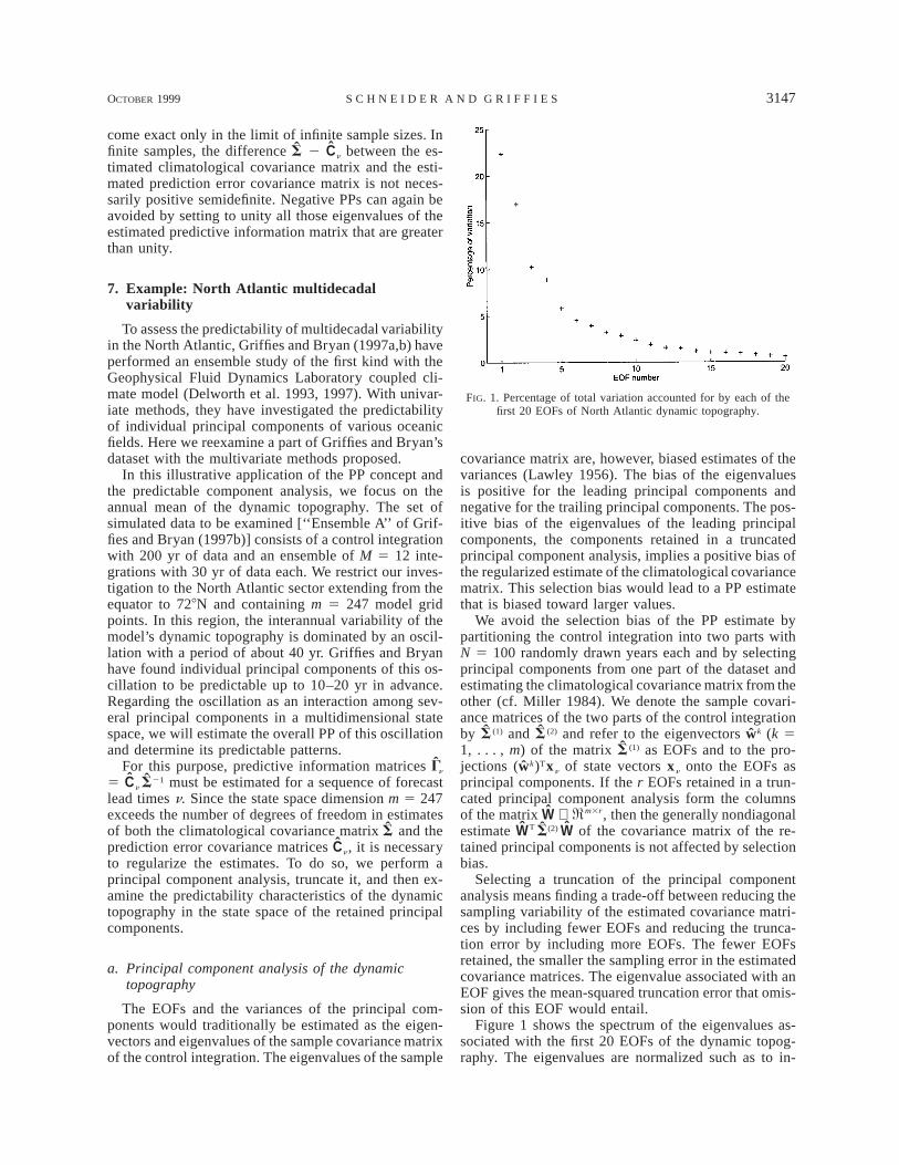
OCTOBER 1999 3147S C H N E I D E R A N D G R I F F I E S
FIG. 1. Percentage of total variation accounted for by each of thefirst 20 EOFs of North Atlantic dynamic topography.
come exact only in the limit of infinite sample sizes. Infinite samples, the difference 2 Cn between the es-Stimated climatological covariance matrix and the esti-mated prediction error covariance matrix is not neces-sarily positive semidefinite. Negative PPs can again beavoided by setting to unity all those eigenvalues of theestimated predictive information matrix that are greaterthan unity.
7. Example: North Atlantic multidecadalvariability
To assess the predictability of multidecadal variabilityin the North Atlantic, Griffies and Bryan (1997a,b) haveperformed an ensemble study of the first kind with theGeophysical Fluid Dynamics Laboratory coupled cli-mate model (Delworth et al. 1993, 1997). With univar-iate methods, they have investigated the predictabilityof individual principal components of various oceanicfields. Here we reexamine a part of Griffies and Bryan’sdataset with the multivariate methods proposed.
In this illustrative application of the PP concept andthe predictable component analysis, we focus on theannual mean of the dynamic topography. The set ofsimulated data to be examined [‘‘Ensemble A’’ of Grif-fies and Bryan (1997b)] consists of a control integrationwith 200 yr of data and an ensemble of M 5 12 inte-grations with 30 yr of data each. We restrict our inves-tigation to the North Atlantic sector extending from theequator to 728N and containing m 5 247 model gridpoints. In this region, the interannual variability of themodel’s dynamic topography is dominated by an oscil-lation with a period of about 40 yr. Griffies and Bryanhave found individual principal components of this os-cillation to be predictable up to 10–20 yr in advance.Regarding the oscillation as an interaction among sev-eral principal components in a multidimensional statespace, we will estimate the overall PP of this oscillationand determine its predictable patterns.
For this purpose, predictive information matrices Gn
5 Cn must be estimated for a sequence of forecast21Slead times n. Since the state space dimension m 5 247exceeds the number of degrees of freedom in estimatesof both the climatological covariance matrix and theSprediction error covariance matrices Cn, it is necessaryto regularize the estimates. To do so, we perform aprincipal component analysis, truncate it, and then ex-amine the predictability characteristics of the dynamictopography in the state space of the retained principalcomponents.
a. Principal component analysis of the dynamictopography
The EOFs and the variances of the principal com-ponents would traditionally be estimated as the eigen-vectors and eigenvalues of the sample covariance matrixof the control integration. The eigenvalues of the sample
covariance matrix are, however, biased estimates of thevariances (Lawley 1956). The bias of the eigenvaluesis positive for the leading principal components andnegative for the trailing principal components. The pos-itive bias of the eigenvalues of the leading principalcomponents, the components retained in a truncatedprincipal component analysis, implies a positive bias ofthe regularized estimate of the climatological covariancematrix. This selection bias would lead to a PP estimatethat is biased toward larger values.
We avoid the selection bias of the PP estimate bypartitioning the control integration into two parts withN 5 100 randomly drawn years each and by selectingprincipal components from one part of the dataset andestimating the climatological covariance matrix from theother (cf. Miller 1984). We denote the sample covari-ance matrices of the two parts of the control integrationby and and refer to the eigenvectors wk (k 5(1) (2)ˆ ˆS S1, . . . , m) of the matrix as EOFs and to the pro-(1)Sjections (wk)Txn of state vectors xn onto the EOFs asprincipal components. If the r EOFs retained in a trun-cated principal component analysis form the columnsof the matrix W ∈ then the generally nondiagonalm3rR ,estimate W of the covariance matrix of the re-T (2)ˆ ˆW Stained principal components is not affected by selectionbias.
Selecting a truncation of the principal componentanalysis means finding a trade-off between reducing thesampling variability of the estimated covariance matri-ces by including fewer EOFs and reducing the trunca-tion error by including more EOFs. The fewer EOFsretained, the smaller the sampling error in the estimatedcovariance matrices. The eigenvalue associated with anEOF gives the mean-squared truncation error that omis-sion of this EOF would entail.
Figure 1 shows the spectrum of the eigenvalues as-sociated with the first 20 EOFs of the dynamic topog-raphy. The eigenvalues are normalized such as to in-

3148 VOLUME 12J O U R N A L O F C L I M A T E
FIG. 2. (a) First EOF and (b) second EOF of North Atlantic dynamictopography [dynamic cm]. The patterns are scaled by the standarddeviations of their associated principal components.
dicate the percentage of total sample variation accountedfor by each of the EOFs. Figure 1 suggests a truncationafter the fourth EOF, at the eigenvalue spectrum’s pointof greatest curvature. However, the third and fourthEOFs represent centennial trends in the model’s deeperocean (Griffies and Bryan 1997b). Since we are inter-ested in multidecadal oscillations and not in long-termmodel trends, we focus on the first two EOFs.
Figure 2 shows the first and second EOF patterns.The EOF patterns, normalized to norm unity, are in thisplot multiplied by the standard deviation of their prin-cipal components, so the amplitude of the patterns in-dicates the rms variability of the dynamic topography.EOF1 represents variations in the strength of the NorthAtlantic Current’s northeastward drift. The dynamic to-pography variations have maximum amplitude in themodel’s western boundary region. EOF2 is more elon-gated meridionally than EOF1, and it extends farthernorthward into the sinking region of the model’s sub-polar North Atlantic. EOF2 represents gyre-shaped var-iations in the North Atlantic circulation with the stron-gest current variations directed northeastward and lo-cated in the central portion of the basin. The principalcomponents associated with these patterns exhibit ir-regular oscillations with a dominant period of 40–45yr. Since the two principal component time series areroughly in quadrature, the EOFs can be viewed as dif-ferent phases of an oscillatory mode of dynamic to-pography variability.
Together, the first two EOFs account for 39% of thetotal sample variation in North Atlantic dynamic to-
pography. In the central and western North Atlantic,where these EOFs have the largest amplitude, the cor-relation coefficients between the principal componenttime series and the local variations in dynamic topog-raphy exceed 0.8 (Griffies and Bryan 1997b). Hence,predictability of the two EOFs would imply predict-ability of a large portion of local variability in thesedynamically active regions.
b. Predictability estimates from the ensembleintegration
To obtain regularized estimates of the predictive in-formation matrices, we project the data from the en-semble integration onto the r 5 2 EOFs retained in thetruncated principal component analysis. For each leadtime n 5 1, . . . , 30 yr, we estimate a prediction errorcovariance matrix Cn ∈ from the sample covariancer3rRmatrix of the residuals (23). The full sample covariancematrix ∈ of N 5 100 yr of the control in-m3m(2)S Rtegration is used in the estimate W ∈T (2)ˆ ˆ ˆS 5 W S
of the climatological covariance matrix in the trun-r3rRcated EOF basis. With the Cholesky factorization tech-nique in the appendix, PPs and the predictable com-ponent analysis are computed from the covariance ma-trices Cn and .S
This approach to estimating the predictive informa-tion matrices avoids selection bias. However, the esti-mation of the climatological covariance matrix drawsupon only 100 yr out of the 200 yr of available data.But since for the estimation of the prediction error co-variance matrices Cn only 11 degrees of freedom areavailable, against 99 degrees of freedom for the esti-mation of the climatological covariance matrix , theSsampling variability of the predictive information ma-trices 5 Cn is dominated by the sampling vari-21ˆ ˆG Sn
ability of the prediction error covariance matrices Cn.Therefore, ignoring one-half of the control integrationin the estimation of the climatological covariance matrixhas little effect on the accuracy of the predictive infor-mation matrix estimates.
Figure 3a shows the overall PP of the first two EOFsas a function of forecast lead time n. At each n weestimate, by Monte Carlo simulation of 1000 samples,a 95% confidence interval for the PP estimate. Each ofthe 1000 samples consists of M 5 12 random vectorsdrawn from a Gaussian distribution with a covariancematrix equal to the sample covariance matrix Cn of theresiduals and N 5 100 random vectors drawn from aGaussian distribution with a covariance matrix equal tothe estimated covariance matrix W of theT (2)ˆ ˆ ˆS 5 W Sprincipal components. A PP is computed from each sam-ple. Adding the difference between the 97.5th percentileand the mean of the simulated PPs to the overall PPgives the upper bound of the estimated 95% confidenceinterval, and subtracting the difference between themean of the simulated PPs and the 2.5th percentile givesthe lower bound. Because the thus estimated 95% con-
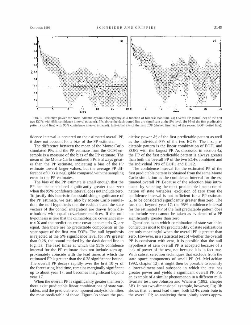
OCTOBER 1999 3149S C H N E I D E R A N D G R I F F I E S
FIG. 3. Predictive power for North Atlantic dynamic topography as a function of forecast lead time. (a) Overall PP (solid line) of the firsttwo EOFs with 95% confidence interval (shaded). PPs above the dash-dotted line are significant at the 5% level. (b) PP of the first predictablepattern (solid line) with 95% confidence interval (shaded). Individual PPs of the first EOF (dashed line) and of the second EOF (dotted line).
fidence interval is centered on the estimated overall PP,it does not account for a bias of the PP estimate.
The difference between the mean of the Monte Carlosimulated PPs and the PP estimate from the GCM en-semble is a measure of the bias of the PP estimate. Themean of the Monte Carlo simulated PPs is always great-er than the PP estimate, indicating a bias of the PPestimate toward larger values, but the average PP dif-ference of 0.03 is negligible compared with the samplingerror in the PP estimates.
The bias of the PP estimate is small enough that thePP can be considered significantly greater than zerowhen the 95% confidence interval does not include zero.To justify this heuristic for establishing significance ofthe PP estimate, we test, also by Monte Carlo simula-tion, the null hypothesis that the residuals and the statevectors of the control integration are drawn from dis-tributions with equal covariance matrices. If the nullhypothesis is true that the climatological covariance ma-trix S and the prediction error covariance matrix Cn areequal, then there are no predictable components in thestate space of the first two EOFs. The null hypothesisis rejected at the 5% significance level for PPs greaterthan 0.28, the bound marked by the dash-dotted line inFig. 3a. The lead times at which the 95% confidenceinterval for the PP estimate does not include zero ap-proximately coincide with the lead times at which theestimated PP is greater than the 0.28 significance bound.The overall PP decays rapidly over the first 10 yr ofthe forecasting lead time, remains marginally significantup to about year 17, and becomes insignificant beyondyear 17.
When the overall PP is significantly greater than zero,there exist predictable linear combinations of state var-iables, and the predictable component analysis identifiesthe most predictable of those. Figure 3b shows the pre-
dictive power of the first predictable pattern as well1an
as the individual PPs of the two EOFs. The first pre-dictable pattern is the linear combination of EOF1 andEOF2 with the largest PP. As discussed in section 4a,the PP of the first predictable pattern is always greaterthan both the overall PP of the two EOFs combined andthe individual PPs of EOF1 and EOF2.
The confidence interval for the estimated PP of thefirst predictable pattern is obtained from the same MonteCarlo simulation as the confidence interval for the es-timated overall PP. Because of the selection bias intro-duced by selecting the most predictable linear combi-nation of state variables, exclusion of zero from theconfidence interval is not sufficient for a PP estimate
to be considered significantly greater than zero. The1an
fact that, beyond year 17, the 95% confidence intervalfor the estimated PP of the first predictable pattern doesnot include zero cannot be taken as evidence of a PPsignificantly greater than zero.
Questions as to which combination of state variablescontributes most to the predictability of state realizationsare only meaningful when the overall PP is greater thanzero. However, in a statistical test of whether the overallPP is consistent with zero, it is possible that the nullhypothesis of zero overall PP is accepted because of alack of power of the test, not because it is in fact true.With subset selection techniques that exclude from thestate space components of small PP (cf. McLachlan1992, chapter 12), it might then be possible to identifya lower-dimensional subspace in which the test hasgreater power and yields a significant overall PP. Foran example of a similar phenomenon in a different mul-tivariate test, see Johnson and Wichern (1982, chapter5B). In our two-dimensional example, however, Fig. 3bshows that, at most lead times, both EOFs contribute tothe overall PP, so analyzing them jointly seems appro-
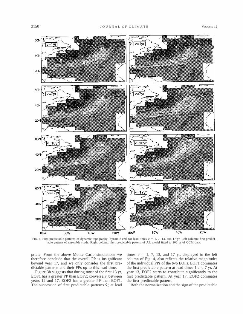
3150 VOLUME 12J O U R N A L O F C L I M A T E
FIG. 4. First predictable patterns of dynamic topography [dynamic cm] for lead times n 5 1, 7, 13, and 17 yr. Left column: first predict-able pattern of ensemble study. Right column: first predictable pattern of AR model fitted to 100 yr of GCM data.
priate. From the above Monte Carlo simulations wetherefore conclude that the overall PP is insignificantbeyond year 17, and we only consider the first pre-dictable patterns and their PPs up to this lead time.
Figure 3b suggests that during most of the first 13 yr,EOF1 has a greater PP than EOF2; conversely, betweenyears 14 and 17, EOF2 has a greater PP than EOF1.The succession of first predictable patterns at lead1vn
times n 5 1, 7, 13, and 17 yr, displayed in the leftcolumn of Fig. 4, also reflects the relative magnitudesof the individual PPs of the two EOFs. EOF1 dominatesthe first predictable pattern at lead times 1 and 7 yr. Atyear 13, EOF2 starts to contribute significantly to thefirst predictable pattern. At year 17, EOF2 dominatesthe first predictable pattern.
Both the normalization and the sign of the predictable
OCTOBER 1999 3151S C H N E I D E R A N D G R I F F I E S
patterns are matters of convention. According to thenormalization convention (16), the predictable patternsare orthogonal with respect to the inverse climatologicalcovariance matrix . Therefore, amplitudes of the pat-21Sterns in Fig. 4 indicate the rms variability of the dynamictopography. The sign of the first predictable pattern
at lead time n is chosen so as to minimize the squared1vn
Mahalanobis distance ( 2 2 ) to the1 1 T 21 1 1ˆv v ) S (v vn n21 n n21
pattern at lead time n 2 1. The first predictable1vv21
pattern at n 5 0 is taken to be the normalized model1v0
state at the initialization of the ensemble integration.This sign convention ensures that the first predictablepatterns evolve smoothly with forecast lead time.
In the initial conditions for the ensemble integration,the Atlantic overturning circulation is anomalouslyweak. Figure 4 shows that what is most predictable 1and 7 yr in advance is the state vector component as-sociated with a weak-drift anomaly in the North AtlanticCurrent. Most predictable 13 yr in advance is the statevector component associated with a spreading of theweak-drift anomaly into subpolar regions and with thebeginning formation of a gyre-shaped current anomalyin the central North Atlantic. Most predictable 17 yr inadvance is the state vector component associated witha decrease in amplitude of the weak-drift anomaly inthe North Atlantic Current and with an increase in am-plitude and a northward spreading of the gyre-shapedanomaly in the central North Atlantic. The first pre-dictable patterns represent those features of the dynamictopography whose components are predictable with thesmallest rms error relative to the rms error of the cli-matological mean prediction.
The examination of the PP, of the significance of thePP, and of the first predictable patterns confirms andcomplements the analyses of Griffies and Bryan(1997b). The results presented above were found to berobust: they do not depend on the particular randompartition of the control integration chosen to estimatethe EOFs and the climatological covariance matrix.
c. Empirical predictability estimates from an ARmodel
Predictability characteristics can also be derived em-pirically from AR models fitted to the same set of GCMdata projected onto two EOFs. The AR model identi-fication is performed with the software package ARFIT
(Schneider and Neumaier 1997).Among AR(p) models of order p 5 0, . . . , 6, the
order selection criteria SBC and MSC indicate that anAR(1) model best fits the first 100 yr of the GCM controlintegration. To check whether the fitted AR(1) model isadequate to represent the GCM data, we test the resid-uals (29) of the fitted model for uncorrelatedness. ForN realizations of a white noise process, approximately95% of the sample autocorrelations are expected to liewithin the bounds 61.96(N)21/2 (e.g., Brockwell andDavis 1991, chapter 7.2). For the 99 bivariate residuals
of the fitted AR(1) model, all but 2 of the 40 sampleautocorrelations between lags 1 and 20 lie within thebounds 61.96(99)21/2. Additionally, the modified port-manteau statistic of Li and McLeod (1981) does notreject, at the 5% significance level, the null hypothesisthat the residuals are uncorrelated. Therefore, within theclass of AR models, an AR(1) model fits the first 100yr of the control integration best; the residuals of thefitted model provide no grounds for rejecting the hy-pothesis that the model is consistent with the GCM data.
The AR model identification procedure was repeatedwith segments of the GCM data of various lengths.AR(1) models were consistently found to be the bestfitting, and diagnostic tests of the fitted models providedno grounds for rejecting the hypothesis of model ade-quacy. But the fact that an AR(1) model seems to rep-resent adequately the particular set of oscillatory prin-cipal component time series considered here is not tobe taken as a justification for the indiscriminate use offirst-order models. The adequacy of a fitted model mustbe assessed, and, when linear stochastic models are atall adequate, then higher-order models will often bemore appropriate than first-order models. [For an ex-ample of how models of inappropriately low order canproduce misleading results, see Tiao and Box (1981).]As discussed in section 6, the PP concept and the pre-dictable component analysis are applicable to AR mod-els of any order.
A x2-test of the skewness and kurtosis of the residuals(29) of the fitted AR(1) model does not reject, at the5% significance level, the hypothesis that the residualsare a realization of a Gaussian process. The estimatorsof the prediction error covariance matrices in section 6bare valid for Gaussian processes and can thus be ex-pected to yield reliable estimates of the PP of the ARmodel (cf. Lutkepohl 1993, chapters 3.5 and 4.5).
Figure 5 shows the PP of the fitted AR(1) model asa function of forecast lead time. Since the predictionerror variance of an AR model is a monotonically in-creasing function of lead time (Lutkepohl 1993, chapter2.2), the PP decreases monotonically. The overall PP ofthe AR(1) model fitted to the first 100 yr of the GCMcontrol integration reaches zero at a lead time of about20 yr. Beyond year 20, the error variances of a modelprediction are estimated to be as large as the error var-iances of the climatological mean prediction.
Included in Fig. 5 is the overall PP of an AR modelfitted to only 30 yr of GCM data. Sampling errors con-tribute to the uncertainty in predictions, and since thesampling errors in models decrease with increasinglength of the time series from which the model param-eters are estimated, the PP of the model fitted to 30 yrof data is smaller than the PP of the model fitted to 100yr of data. The PP of the model fitted to 30 yr of dataalready vanishes at a lead time of 11 yr. However, ifsampling errors in the estimated parameters are not tak-en into account and the PP is estimated only from thegeneric prediction error matrices and , then themod modˆ ˆC Sn

3152 VOLUME 12J O U R N A L O F C L I M A T E
FIG. 5. Here, PP of AR models as a function of forecast lead time:overall PP (solid line) and PP of first predictable pattern (dash-dottedline) of AR model fitted to 100 yr of GCM data; overall PP of ARmodel fitted to 30 yr of GCM data (dashed line).
PPs of the two AR models are almost indistinguishableand nonzero up to year 40. Therefore, the differencebetween the two PP curves in Fig. 5 can be attributedentirely to larger sampling errors in the parameters ofthe model fitted to the shorter time series. Neglectingsampling errors leads to a gross overestimation of thepredictive capabilities of fitted AR models.
The PP of the first predictable pattern of the AR(1)model fitted to 100 yr of GCM data is shown in Fig. 5,and the right column of Fig. 4 displays the first pre-dictable pattern itself. The sign and normalization con-ventions of section 7b are applied. The qualitative fea-tures of the first predictable patterns of the AR modelare the same as those of the first predictable patternsinferred from the ensemble integration. Since the pre-dictive information matrix of an AR model does notdepend on the initial condition for a prediction, the sig-nificance of the agreement between the first predictablepatterns inferred from the ensemble integration and fromthe AR model goes beyond indicating that the AR modelfits the GCM data well. At lead time 1 year, the firstpredictable pattern of the AR model is dominated bythe anomaly, represented by EOF1, in the strength ofthe North Atlantic Current’s northeastward drift. Thispattern suggests that predictions of the AR model areparticularly reliable when initialized during either anextremely strong or an extremely weak phase of theoscillation in the strength of this drift. The GCM en-semble was initialized during an extremely weak phaseof the North Atlantic Current, which explains the agree-ment between the predictable patterns.
Thus, the estimation of predictability characteristicsfrom the ensemble integration and from an AR modelfitted to a small fraction of the GCM data leads to similarresults. For the GCM and the AR model, the lead-timescales over which the overall PP is distinguishable from
zero coincide, and the same features of the dynamictopography field are associated with large PP. Such anagreement of results is possible if, as in our example,the process in question can be modeled as a linear su-perposition of stochastically forced damped-oscillatoryand relaxatory modes, modes that an AR model is ableto represent.
8. Concluding remarks
We have presented a conceptual framework for themultivariate analysis of predictability studies. The pre-dictability measure in this framework, the PP, indicatesby how much a prediction reduces the uncertainty as towhich state of the predicted process will occur. Theuncertainties in the state before and after a specific pre-diction is made are quantified by the prior entropy andthe posterior entropy. The difference between these twoentropies is the predictive information contained in aprediction. The PP, an index between zero and one, isbased on an exponential of the predictive informationand measures the efficacy of predictions in narrowingthe range of values typically taken by state vector com-ponents.
To quantify predictability, the information content ofpredictions must be measured relative to the backgroundinformation available prior to the issue of a prediction.Since climatological statistics are accessible in the typesof predictability studies discussed in this paper, wechose to measure the predictive power of predictionsrelative to the climatological mean prediction as a base-line. The prior entropy thus became the entropy of theclimatological distribution of states, or the entropy ofthe distribution of errors in the climatological mean pre-diction. Other choices of a baseline are, however, pos-sible. To evaluate the performance of weather fore-casting models, for example, one might choose the per-sistence forecast as a baseline. The methods presentedabove can then be applied with the prediction error ofthe persistence forecast substituted for the predictionerror of the climatological mean prediction.
For Gaussian random variables, the PP is a functionof the determinant of the predictive information matrix,the product matrix of the prediction error covariancematrix and the inverse of the climatological covariancematrix. Estimating the PP thus reduces to estimating thepredictive information matrix from samples of data orfrom estimated parameters of empirical models. Wehave discussed how the predictive information matrixis obtained from ensemble integration studies of the firstand the second kind and from AR models fitted to ob-served or simulated data. The application of the PP con-cept in an ensemble integration study of the predict-ability of multidecadal North Atlantic variability illus-trates how confidence intervals and significance boundsfor the PP estimate can be established and how the PPis to be interpreted.
When the estimated PP of a process is significantly

OCTOBER 1999 3153S C H N E I D E R A N D G R I F F I E S
greater than zero, the process has predictable compo-nents, and these can be discriminated from the unpre-dictable components by a predictable component anal-ysis, an eigendecomposition of the predictive infor-mation matrix. If state vectors are expanded in terms ofpredictable patterns—that is, in terms of the right ei-genvectors of the predictive information matrix—thentheir first component is the most predictable, and sub-sequent components are mutually uncorrelated and or-dered by PP from largest to smallest. The examinationof North Atlantic variability illustrates the interpretationof the first predictable pattern. The sequence of pre-dictable patterns for forecast lead times between 1 and17 yr shows the most predictable features of a multi-decadal oscillation in the dynamic topography field. Inthis example, the analysis of an AR model adequatelyrepresenting the oscillation in the dynamic topographyand the analysis of an ensemble of GCM integrationsyield similar lead-time scales of nonzero PP and similarpredictable patterns.
Although the PP and the predictable component anal-ysis have been derived under the assumption that thestates and prediction errors follow Gaussian distribu-tions, it is the ellipsoidal symmetry of the distributionsthat is more important than their detailed shape (Fried-man 1989). Hence, the assumption of Gaussian distri-butions can, in practice, be relaxed to a symmetry as-sumption.
The framework that has been presented in this paperis applicable to a wider range of studies than that ex-plicitly covered. The above-mentioned performanceevaluation of weather forecasting models is but one ex-ample of further applications. Grounding our analysesin the literature on multivariate statistics will, we hope,facilitate the extension of the framework to other ap-plications.
Acknowledgments. We wish to express our thanks toJeff Anderson and Arnold Neumaier, who drew our at-tention to some of the referenced literature on climaticpredictability and discriminant analysis, respectively.Jeff Anderson, Ruth Michaels, Thomas Muller, ArnoldNeumaier, Heidi Swanson, and Jens Timmer carefullyread drafts of this paper. We gratefully acknowledgetheir comments and criticism, which led to substantialimprovements in the final version.
APPENDIX
Computation of the Predictable ComponentAnalysis
The predictable component analysis simultaneouslydiagonalizes the climatological covariance matrix andthe prediction error covariance matrix. This fact can beexploited in the practical computation of predictablecomponents and predictable patterns (cf. Fukunaga1990, chapter 2).
First, we compute the principal component analysisSn 5 Wn Ln of the climatological covariance matrixTWn
Sn. The orthogonal matrix Wn, whose columns are theeigenvectors of Sn, and the diagonal eigenvalue matrixLn 5 Diag( ) are then used in a whitening transfor-kln
mation (18), which transforms the climatological co-variance matrix into the identity matrix and the predic-tion error covariance matrix into the matrix Kn given in(19). The matrix Kn is symmetric but not necessarilydiagonal. It can be diagonalized by a further orthogonaltransformation Tn, with columns of Tn formed by eigen-vectors of Kn, such that, as in (14),
Cn Wn Tn 5 KnTn 5 Diag( ).T T T21/2 21/2 kT L W L T gn n n n n n
(A1)
The identity matrix (18) remains unchanged under thistransformation:
Sn Wn Tn 5 I Tn 5 I.T T T21/2 21/2T L W L Tn n n n n (A2)
Comparing the expressions (A1) and (A2) for the trans-formed covariance matrices with the corresponding ex-pressions (14) and (13) in the predictable pattern basis,we obtain for the weight vector matrix
Un 5 Wn Tn.21/2Ln (A3)
From the biorthogonality condition (9) follows
Vn 5 Wn Tn1/2Ln (A4)
for the matrix Vn with predictable patterns as columns.The implementation of this algorithm can be checkedfor consistency by verifying that the weight vector ma-trix Un and the predictable pattern matrix Vn satisfy thecompleteness and biorthogonality conditions (9).
If the climatological covariance matrix Sn is singular,one or more of the eigenvalues in Ln 5 Diag( ) isk kl ln n
zero and 5 Diag[( )21/2] does not exist. Regu-21/2 kL ln n
larization by truncated principal component analysisproceeds by setting to zero both the eigenvalues notkln
significantly different from zero and the square root( )21/2 of their inverses. Zeroing these contributions tokln
the inverse climatological covariance matrix 5 Wn21Sn
amounts to replacing the ill-defined inverseT21L Wn n
by a Moore–Penrose pseudoinverse (see, e.g., Go-21Sn
lub and van Loan 1993, chapter 5). If, after regulari-zation, only the first r of the m eigenvalues are non-kln
zero, the predictable component analysis is computedin the truncated r-dimensional state space.
Computing the predictable component analysis by aprincipal component analysis of the climatological co-variance matrix Sn followed by a principal componentanalysis of the prediction error covariance matrix Kn hasseveral advantages: besides the predictable patterns Vn,it produces the EOFs Wn; and the predictable componentanalysis can be regularized by truncating the principalcomponent analysis of the climatological covariancematrix. However, when no regularization needs to beperformed, it is numerically more efficient to replacethe eigendecomposition Sn 5 Wn Ln of the clima-TWn

3154 VOLUME 12J O U R N A L O F C L I M A T E
tological covariance matrix by a Cholesky decomposi-tion Sn 5 Ln and to use the Cholesky factor Ln inTLn
place of Wn and in place of Wn (Press et2T1/2 21/2L L Ln n n
al. 1992, 455).In predictability studies of the first kind, the clima-
tological covariance matrix Sn usually does not dependon the forecast lead time n, so that the whitening trans-formation (18) with the matrix or with theT21/2L Wn n
Cholesky factor need be computed only once. Only21Ln
the eigendecomposition Tn of the transformed predictionerror covariance matrix Kn must be computed for eachforecast lead time n. In predictability studies of the sec-ond kind, all of the above transformations must be com-puted for each time n for which a prediction is made.
REFERENCES
Ahmad, T. A., and P.-E. Lin, 1976: A nonparametric estimation ofthe entropy for absolutely continuous distributions. IEEE Trans.Inf. Theory, 22, 372–375.
Anderson, J. L., and W. F. Stern, 1996: Evaluating the potential pre-dictive utility of ensemble forecasts. J. Climate, 9, 260–269.
Anderson, T. W., 1984: An Introduction to Multivariate StatisticalAnalysis. 2d ed. Series in Probability and Mathematical Statis-tics, Wiley, 675 pp.
Ansley, C. F., and R. Kohn, 1983: Exact likelihood of a vector au-toregressive moving average process with missing or aggregateddata. Biometrika, 70, 275–278., and , 1986: A note on reparameterising a vector autore-gressive moving average model to enforce stationarity. J. Stat.Comput. Sim., 24, 99–106.
Bell, T. L., 1982: Optimal weighting of data to detect climatic change:Application to the carbon dioxide problem. J. Geophys. Res.,87, 11 161–11 170., 1986: Theory of optimal weighting of data to detect climaticchange. J. Atmos. Sci., 43, 1694–1710.
Box, G. E. P., and G. C. Tiao, 1977: A canonical analysis of multipletime series. Biometrika, 64, 355–365.
Brillouin, L., 1956: Science and Information Theory. Academic Press,320 pp.
Brockwell, P. J., and A. Davis, 1991: Time Series: Theory and Meth-ods. 2d ed. Springer, 577 pp.
Cheng, Y.-Q., Y.-M. Zhuang, and J.-Y. Yang, 1992: Optimal Fisherdiscriminant analysis using the rank decomposition. Pattern Re-cognit., 25, 101–111.
Delworth, T., S. Manabe, and R. J. Stouffer, 1993: Interdecadal var-iations of the thermohaline circulation in a coupled ocean–at-mosphere model. J. Climate, 6, 1993–2011., , and , 1997: Multidecadal climate variability in theGreenland Seas and surrounding regions: A coupled model sim-ulation. Geophys. Res. Lett., 24, 257–260.
Dmitriev, Y. G., and F. P. Tarasenko, 1973: On the estimation offunctionals of the probability density and its derivatives. TheoryProbab. Appl., 18, 628–633.
Draper, D., 1995: Assessment and propagation of model uncertainty.J. Roy. Stat. Soc. B, 57, 45–97.
Engl, H. W., M. Hanke, and A. Neubauer, 1996: Regularization ofInverse Problems. Kluwer, 321 pp.
Friedman, J. H., 1989: Regularized discriminant analysis. J. Amer.Stat. Assoc., 84, 165–175.
Fukunaga, K., 1990: Introduction to Statistical Pattern Recognition.2d ed. Academic Press, 591 pp.
Golub, G. H., and C. F. van Loan, 1993: Matrix Computations. 2ded. Johns Hopkins University Press, 642 pp.
Griffies, S. M., and K. Bryan, 1997a: Predictability of North Atlanticmultidecadal climate variability. Science, 275, 181–184.
, and , 1997b: A predictability study of simulated NorthAtlantic multidecadal variability. Climate Dyn., 8, 459–488.
Hall, P., and S. C. Morton, 1993: On the estimation of entropy. Ann.Inst. Stat. Math., 45, 69–88.
Halliwell, G. R., 1997: Decadal and multidecadal North Atlantic SSTanomalies driven by standing and propagating basin-scale at-mospheric anomalies. J. Climate, 10, 2405–2411., 1998: Simulation of North Atlantic decadal/multidecadal winterSST anomalies driven by basin-scale atmospheric circulationanomalies. J. Phys. Oceanogr., 28, 5–21.
Hansen, P. C., 1997: Rank-Deficient and Discrete Ill-Posed Problems:Numerical Aspects of Linear Inversion. SIAM Monogr. on Math-ematical Modeling and Computation, Society for Industrial andApplied Mathematics, 247 pp.
Harzallah, A., and R. Sadourny, 1995: Internal versus SST-forcedatmospheric variability as simulated by an atmospheric circu-lation model. J. Climate, 8, 474–495.
Hasselmann, K., 1993: Optimal fingerprints for the detection of time-dependent climate change. J. Climate, 6, 1957–1971.
Hayashi, Y., 1986: Statistical interpretation of ensemble-time meanpredictability. J. Meteor. Soc. Japan, 64, 167–181.
Hegerl, G. C., and G. R. North, 1997: Comparison of statisticallyoptimal approaches to detecting anthropogenic climate change.J. Climate, 10, 1125–1133.
Joe, H., 1989: Estimation of entropy and other functionals of a mul-tivariate density. Ann. Inst. Stat. Math., 41, 683–697.
Johnson, R. A., and D. W. Wichern, 1982: Applied Multivariate Sta-tistical Analysis. Prentice-Hall, 594 pp.
Jolliffe, I. T., 1986: Principal Component Analysis. Springer Seriesin Statistics, Springer, 271 pp.
Krzanowski, W. J., P. Jonathan, W. V. McCarthy, and M. R. Thomas,1995: Discriminant analysis with singular covariance matrices:Methods and applications to spectroscopic data. Appl. Stat. 44,101–115.
Lawley, D. N., 1956: Tests of significance for the latent roots ofcovariance and correlation matrices. Biometrika, 43, 128–136.
Li, W. K., and A. I. McLeod, 1981: Distribution of the residual au-tocorrelations in multivariate ARMA time series models. J. Roy.Stat. Soc. B, 43, 231–239.
Lorenz, E. N., 1963: Deterministic nonperiodic flow. J. Atmos. Sci.,20, 130–141., 1975: Climatic predictability. The Physical Basis of Climateand Climate Modelling, B. Bolin et al., Eds., GARP PublicationSeries, Vol. 16, World Meteorological Organization, 132–136.
Lutkepohl, H., 1985: Comparison of criteria for estimating the orderof a vector autoregressive process. J. Time Ser. Anal., 6, 35–52;Correction, 8, 373., 1993: Introduction to Multiple Time Series Analysis. 2d ed.Springer-Verlag, 545 pp.
McLachlan, G. J., 1992: Discriminant Analysis and Statistical PatternRecognition. Series in Probability and Mathematical Statistics,Wiley, 544 pp.
Miller, A. J., 1984: Selection of subsets of regression variables. J.Roy. Stat. Soc. A, 147, 389–425.
Murphy, J. M., 1988: The impact of ensemble forecasts on predict-ability. Quart. J. Roy. Meteor. Soc., 114, 463–493.
Neumaier, A., 1998: Solving ill-conditioned and singular linear sys-tems: A tutorial on regularization. SIAM Rev., 40, 636–666., and T. Schneider, cited 1997: Multivariate autoregressive and Orn-stein–Uhlenbeck processes: Estimates for order, parameters, spectralinformation, and confidence regions. [Available online at http://www.aos.Princeton.EDU/WWWPUBLIC/tapio/arfit/.]
Palmer, T. N., 1996: Predictability of the atmosphere and oceans:From days to decades. Decadal Climate Variability: Dynamicsand Predictability, D. L. T. Anderson and J. Willebrand, Eds.,NATO ASI Series, Vol. I 44, Springer, 83–155., R. Gelaro, J. Barkmeijer, and R. Buizza, 1998: Singular vectors,metrics, and adaptive observations. J. Atmos. Sci., 55, 633–653.
Papoulis, A., 1991: Probability, Random Variables, and StochasticProcesses. 3d ed. McGraw-Hill, 666 pp.

OCTOBER 1999 3155S C H N E I D E R A N D G R I F F I E S
Prakasa Rao, B. L. S., 1983: Nonparametric Functional Estimation.Series in Probability and Mathematical Statistics, AcademicPress, 522 pp.
Press, W. H., S. A. Teukolsky, W. T. Vetterling, and B. P. Flannery,1992: Numerical Recipes. 2d ed. Cambridge University Press,963 pp.
Ripley, B. D., 1996: Pattern Recognition and Neural Networks. Cam-bridge University Press, 403 pp.
Schneider, T., and A. Neumaier, cited 1997: Algorithm: ARfit—AMatlab package for estimation and spectral decomposition ofmultivariate autoregressive processes. [Available online at http://www.aos.Princeton.EDU/WWWPUBLIC/tapio/arfit/.]
Schwarz, G., 1978: Estimating the dimension of a model. Ann. Stat.,6, 461–464.
Scott, D. W., 1992: Multivariate Density Estimation: Theory, Prac-tice, and Visualization. Series in Probability and MathematicalStatistics, Wiley, 317 pp.
Shannon, C. E., 1948: A mathematical theory of communication. BellSyst. Tech. J., 27, 370–423, 623–656., and W. Weaver, 1949: The Mathematical Theory of Commu-nication. University of Illinois Press, 117 pp.
Shukla, J., 1981: Dynamical predictability of monthly means. J. At-mos. Sci., 38, 2547–2572., 1985: Predictability. Advances in Geophysics, Vol. 28b, Aca-demic Press, 87–122.
Silverman, B. W., 1986: Density Estimation for Statistics and DataAnalysis. Chapman and Hall, 175 pp.
Stern, W. F., and K. Miyakoda, 1995: The feasibility of seasonalforecasts inferred from multiple GCM simulations. J. Climate,8, 1071–1085.
Thacker, W. C., 1996: Metric-based principal components: Data un-certainties. Tellus, 48A, 584–592.
Tiao, G. C., and G. E. P. Box, 1981: Modeling multiple time serieswith applications. J. Amer. Stat. Assoc., 76, 802–816.
Tikhonov, A. N., and V. Y. Arsenin, 1977: Solution of Ill-Posed Prob-lems. Scripta Series in Mathematics, V. H. Winston and Sons,258 pp.
Toth, Z., 1991: Circulation patterns in phase space: A multinormaldistribution? Mon. Wea. Rev., 119, 1501–1511.
Zwiers, F. W., 1996: Interannual variability and predictability in anensemble of AMIP climate simulations conducted with the CCCGCM2. Climate Dyn., 12, 825–848.