A Conceptual Dynamic Model for Electronic Braking System
9
AEA – Brazilian Society of Automotive Engineering - SIMEA 2021 (Allowed reproduction with source mention: AEA – Simpósio Internacional de Engenharia Automotiva – SIMEA 2021 – São Paulo, Brasil) A Conceptual Dynamic Model for Electronic Braking System Lucas Barbosa de Miguel¹, Armando Antônio Maria Laganá¹, Evandro Leonardo Silva Teixeira², Diego Colón¹, Eduardo Sánchez Cidrón¹ ¹Escola Politécnica da Universidade de São Paulo (EPUSP), ²Universidade de Brasília (FGA) ABSTRACT Advanced Driver Assistance Systems (ADAS) has been one of the fastest-growing sectors in the automotive industry. They are particularly designed to increase car safety and also driving comfort and experience. ADAS technologies embrace many functions like Cruise Control (CC), Adaptive Cruise Control (ACC), Electronic Stability Control (ESC), Assistant Parking System (APS), Lane Keeping Assistant (LKA), Anti-lock Brake System (ABS), among others. Distributed under several networked control modules, those functions acquire sensor data continuously to predict undesired situations and acting on vehicle subsystems on avoiding unsafe and uncomfortable driving conditions. One of the most promising ADAS to prevent or mitigate the severity of a crash is the Electronic Braking System (EBS). An EBS acts to optimize drive and braking operation adjusting braking force and torque for each respective braking situation. It receives sensor data (i.e., radar and/or camera) to detect front objects, braking distance, and speed acting once unsafe conditions are detected. Taking into account the importance of EBS function, this paper aims to design a parameterized dynamic model (PDM) of the automobile braking systems with ABS/ESC functionalities. In particular, this paper highlights the development of modelling equations for each braking system components (from brake pedal up to caliper assembly). The proposed model will be designed and implemented using Matlab/Simulink integrated environment. Simulation and test bench outcomes highlight successful results to represent the Fiat Strada brake systems with ESC support. Keywords: Eletronic Braking, Dynamic Model, Simulation, ABS/ESC. RESUMO O Advanced Driver Assistance Systems (ADAS) tem sido um dos setores de crescimento mais rápido na indústria automotiva. Eles são especialmente promovidos para aumentar a segurança do carro e também o conforto e a experiência de direção. As tecnologias ADAS abrangem muitas funções como Cruise Control (CC), Adaptive Cruise Control (ACC), Electronic Stability Control (ESC), Assistant Parking System (APS), Lanekeeping Assistant (LKA), Antibloqueio Brake System (ABS), entre outras. Distribuídas em vários módulos de controle em rede, essas funções adquirem dados do sensor continuamente para prever indesejadas e atuando nos subsistemas evitando condições de direção inseguras e desconfortáveis. Um dos ADAS mais promissores para prevenir ou mitigar a gravidade de uma colisão é o Sistema de Frenagem Eletrônico (EBS). Um EBS atua para otimizar uma operação de tração e frenagem, ajustando a força e o torque de frenagem para cada situação de frenagem. Ele recebe dados do sensor (ou seja, radar e / ou câmera) para detectar objetos frontais, distância de frenagem e velocidade agindo assim que condições inseguras são detectadas. Levando em consideração a importância da função EBS, este trabalho tem como objetivo o projeto de modelo dinâmico parametrizado (PDM) dos sistemas de frenagem de automóveis com características ABS / ESC. Em particular, este destaca o desenvolvimento das equações de modelagem para cada componente do sistema de frenagem (desde o pedal do freio até a montagem da pinça). O modelo proposto escolhido e implementado em ambiente integrado Matlab / Simulink. Os resultados da simulação e da bancada de teste destacam os resultados bem-sucedidos para representar os sistemas de freio Fiat Strada com suporte ESC. Palavras Chave: Frenagem Eletrônica, Modelo Dinâmico, Simulação, ABS/ESC. INTRODUCTION The braking system is a crucial vehicle safety system to stop the car according to the driver's intention without losing control of the vehicle. Functions such as ACC and ESC have been increasingly common with the responsibility of keeping the vehicle at a safe distance from the vehicle in front ensuring stability, avoiding loss of control, among other functions. This paper introduces a conceptual non-linear Dynamic Model, in order to improve the understanding of the braking system as a whole so that it is possible to perform an electronic braking through an ABS/ESC module, motivated by its use in vehicles equipped with the ADAS system. and in autonomous cars.
Transcript of A Conceptual Dynamic Model for Electronic Braking System

AEA – Brazilian Society of Automotive Engineering - SIMEA 2021
(Allowed reproduction with source mention: AEA – Simpósio Internacional de Engenharia Automotiva – SIMEA 2021 – São Paulo, Brasil)
A Conceptual Dynamic Model for Electronic Braking System
Lucas Barbosa de Miguel¹, Armando Antônio Maria Laganá¹, Evandro Leonardo Silva Teixeira²,
Diego Colón¹, Eduardo Sánchez Cidrón¹ ¹Escola Politécnica da Universidade de São Paulo (EPUSP), ²Universidade de Brasília (FGA)
ABSTRACT
Advanced Driver Assistance Systems (ADAS) has
been one of the fastest-growing sectors in the automotive
industry. They are particularly designed to increase car
safety and also driving comfort and experience. ADAS
technologies embrace many functions like Cruise Control
(CC), Adaptive Cruise Control (ACC), Electronic Stability
Control (ESC), Assistant Parking System (APS), Lane
Keeping Assistant (LKA), Anti-lock Brake System (ABS),
among others. Distributed under several networked control
modules, those functions acquire sensor data continuously to
predict undesired situations and acting on vehicle
subsystems on avoiding unsafe and uncomfortable driving
conditions. One of the most promising ADAS to prevent or
mitigate the severity of a crash is the Electronic Braking
System (EBS). An EBS acts to optimize drive and braking
operation adjusting braking force and torque for each
respective braking situation. It receives sensor data (i.e.,
radar and/or camera) to detect front objects, braking
distance, and speed acting once unsafe conditions are
detected. Taking into account the importance of EBS
function, this paper aims to design a parameterized dynamic
model (PDM) of the automobile braking systems with
ABS/ESC functionalities. In particular, this paper highlights
the development of modelling equations for each braking
system components (from brake pedal up to caliper
assembly). The proposed model will be designed and
implemented using Matlab/Simulink integrated
environment. Simulation and test bench outcomes highlight
successful results to represent the Fiat Strada brake systems
with ESC support.
Keywords: Eletronic Braking, Dynamic Model, Simulation,
ABS/ESC.
RESUMO
O Advanced Driver Assistance Systems (ADAS) tem
sido um dos setores de crescimento mais rápido na indústria
automotiva. Eles são especialmente promovidos para
aumentar a segurança do carro e também o conforto e a
experiência de direção. As tecnologias ADAS abrangem
muitas funções como Cruise Control (CC), Adaptive Cruise
Control (ACC), Electronic Stability Control (ESC),
Assistant Parking System (APS), Lanekeeping Assistant
(LKA), Antibloqueio Brake System (ABS), entre outras.
Distribuídas em vários módulos de controle em rede, essas
funções adquirem dados do sensor continuamente para
prever indesejadas e atuando nos subsistemas evitando
condições de direção inseguras e desconfortáveis. Um dos
ADAS mais promissores para prevenir ou mitigar a
gravidade de uma colisão é o Sistema de Frenagem
Eletrônico (EBS). Um EBS atua para otimizar uma operação
de tração e frenagem, ajustando a força e o torque de
frenagem para cada situação de frenagem. Ele recebe dados
do sensor (ou seja, radar e / ou câmera) para detectar objetos
frontais, distância de frenagem e velocidade agindo assim
que condições inseguras são detectadas. Levando em
consideração a importância da função EBS, este trabalho tem
como objetivo o projeto de modelo dinâmico parametrizado
(PDM) dos sistemas de frenagem de automóveis com
características ABS / ESC. Em particular, este destaca o
desenvolvimento das equações de modelagem para cada
componente do sistema de frenagem (desde o pedal do freio
até a montagem da pinça). O modelo proposto escolhido e
implementado em ambiente integrado Matlab / Simulink. Os
resultados da simulação e da bancada de teste destacam os
resultados bem-sucedidos para representar os sistemas de
freio Fiat Strada com suporte ESC.
Palavras Chave: Frenagem Eletrônica, Modelo Dinâmico,
Simulação, ABS/ESC.
INTRODUCTION
The braking system is a crucial vehicle safety system to
stop the car according to the driver's intention without losing
control of the vehicle. Functions such as ACC and ESC have
been increasingly common with the responsibility of keeping
the vehicle at a safe distance from the vehicle in front
ensuring stability, avoiding loss of control, among other
functions.
This paper introduces a conceptual non-linear Dynamic
Model, in order to improve the understanding of the braking
system as a whole so that it is possible to perform an
electronic braking through an ABS/ESC module, motivated
by its use in vehicles equipped with the ADAS system. and
in autonomous cars.

AEA – Brazilian Society of Automotive Engineering - SIMEA 2021
2
LITERATURE REVIEW
The ADAS concept has been discussed for more than
40 years, in the 1980s and 1990s the Platoon concept was
presented, which is the concept of a platoon of vehicles
guided by a leading vehicle, where the leading car gradually
increased its speed and the platoon of vehicles followed this
increase in speed [1], another proposal was for a platoon of
vehicles that suggested the possibility of an automated
highway and the Platoon would be guided through that
highway, with the possibility of changing lanes for the entire
platoon [2].
Currently, concepts such as autonomous vehicles and
ACC are already well consolidated in the automotive
environment, with several sensors and cameras around the
car so that a good reading of the environment in which it is
located is made so that a good strategy for driving the vehicle
can be drawn up [3] acting on the accelerator, engine torque,
brake, and other parameters.
The automotive braking system consists of mechanical,
hydraulic and electronic components, where ABS is the
electronic component that has access to the vehicle's four-
wheel valves, which makes it the main element for carrying
out a control strategy and maintaining the system original car
braking [1] [2] [3] [4].
SYSTEM MODELING
In light vehicles, an electronic braking system is often
made up by the following components (see Figure 1):
Figure 1 - Automotive braking system [5]
Taking into account those components, we can
represent them as a physical model of the system can be seen
in figure 2, adapted from [2]:
Figure 2 - Physical model of the braking system
Components usually found on braking system are: (1)
brake pedal; (2) brake booster; (3) master cylinder; (4) oil
tank; (5) ABS / ESC module; (6) throttle, which can be rigid
and flexible; (7) wheel brake, which can be brake caliper or
drum brake. Following this physical representation, a
conceptual non-linear mathematical model was designed to
improve the understanding of the braking system.
BRAKE PEDAL - The brake pedal is the interface
between the driver and the braking system. It uses the
principle of the lever as the first multiplier of the force
applied by the driver on the pedal. We represent the force of
the driver by applying a signal with a constant steady-state
gain (K) and a time constant 𝜏𝑝. Regardless of mechanical
delays that may occur and the driver's reaction delay, we can
define brake pedal force using the following equation [1]:
𝐹𝑝 =𝐾
1 + 𝜏𝑝𝑠 (1)
The representation of the pedal is seen in Figure 3:
Figure 3 - Brake pedal free body diagram [1]
Described by the following equation [1]:

AEA – Brazilian Society of Automotive Engineering - SIMEA 2021
3
𝐹𝑜𝑢𝑡
𝐹𝑝=
𝑙𝑎
𝑙𝑏= 𝑔𝑝
(2)
Where: 𝐹𝑝 is the brake pedal force, 𝐹_𝑜𝑢𝑡 is the output
force multiplied by the gain 𝑔𝑝.
BRAKE BOOSTER - The brake booster is the second
force multiplier of the braking system, it is a component
divided into two chambers by a diaphragm in which the first
chamber has atmospheric pressure and in the second
chamber it has a vacuum from the engine intake manifold,
and it is precisely this pressure difference between the
chambers that is responsible for the multiplication of the
input force, which can be described by the following
equation [1]:
𝐹𝑚 =𝐾𝑎
1 + 𝜏𝑎𝑠𝐹𝑜𝑢𝑡
(3)
Where: 𝐾𝑎 is the stationary gain, 𝜏𝑎 is the time constant
and 𝐹𝑚 is the force transferred by the brake booster to the
master cylinder.
MASTER CYLINDER - The function of the master
cylinder is to convert the brake force applied by the driver to
the brake pedal and convert it into proportional hydraulic
pressure [9]. The hydraulic fluid ducts are divided into two
circuits, and the master cylinder, in turn, has two pressure
chambers, each responsible for feeding a hydraulic fluid
circuit. The physical representation of the master cylinder
can be seen in Figure 4 (adapted from [2]):
Figure 4 - Representation of the physical model of the
master cylinder (adapted from [2])
The master cylinder has axial dynamics described as a
system with two degrees of freedom [5], but since 𝑥1 is the
displacement of the primary piston, which is directly
connected to the pressure rod of the brake booster, represent
an input, so the system becomes only a degree of freedom.
With a single equation of states described as [2]:
𝑆(𝑃1 − 𝑃2) − 𝐹𝑓2𝑠𝑛𝑔�̇�2 + 𝑏1(�̇�1 − �̇�2)
+ 𝑘1(𝑥1 − 𝑥2) − 𝑏2�̇�2 − 𝑘2𝑥2
= 𝑚2�̈�2 (4)
Where: S is the hydraulic cylinder surface, 𝑘𝑖 is the
stiffness of the 𝑖𝑡ℎ chamber spring of the cylinder, 𝑏𝑖 is the
oil viscous damping coefficient of the 𝑖𝑡ℎ chamber, 𝑚𝑖 is the
mass of the cylinder of the 𝑖𝑡ℎ chamber, 𝑃𝑖 is the pressure
inside the 𝑖𝑡ℎ chamber and 𝐹𝑓2 is Coulomb's friction
coefficient. The volume of the two chambers of the master
cylinder varies according to the performance of the brake
pedal, and can be described using the following equations
[2]:
𝑉1 = 𝑉10 + 𝑆(𝑥2 − 𝑥1) (5)
𝑉2 = 𝑉20 − 𝑆𝑥2 (6)
Where: 𝑉10 and 𝑉20 are the initial volumes of the first
and second chamber respectively.
ABS MODULE - The ABS module avoids the locking
of the car wheels using a magnetic wheel sensor, a hydraulic
pressure modulator with a pair of valves for each wheel, and
an electronic control unit. So far, many vehicles now have
electronic stability control. In these cases, the hydraulic
modulator has four more valves to perform the stability
control, and for the strategy to be effective, it is necessary to
add other sensors and actuators, such as steering angle
sensor, yaw sensor, pressure sensor, among others. The ABS
/ ESC module is responsible for controlling the valve set of
the hydraulic pressure modulator. It can be seen in its
physical representation in Figure 5:
Figure 5 - Representation of the physical model of the ABS /
ESC hydraulic module
The hydraulic fluid transfers the pressure from the
master cylinder to the brake caliper, and this pressure is
transferred through the flow rate 𝑄𝑖, which is the volumetric
capacity of fluid that passes through a pipe in a unit of time
considered and is described like [1] [2] [3] [4]:
𝑄𝑖𝑛 = 𝐶𝑞𝑖𝑛𝐴𝑖𝑛√2|𝑝1 − 𝑝𝑏|
𝜌𝑠𝑔𝑛(𝑝1 − 𝑝𝑏)
(7)

AEA – Brazilian Society of Automotive Engineering - SIMEA 2021
4
𝑄𝑜𝑢𝑡 = 𝐶𝑞𝑜𝑢𝑡𝐴𝑜𝑢𝑡√2|𝑝𝑏 − 𝑝𝑎|
𝜌𝑠𝑔𝑛(𝑝𝑏 − 𝑝𝑎)
(8)
𝑄𝐹𝐿 = 𝐶𝑞𝐹𝐿𝐴𝐹𝐿√2|𝑝1 − 𝑝𝐹𝐿|
𝜌𝑠𝑔𝑛(𝑝1 − 𝑝𝐹𝐿)
(9)
𝑄𝑒𝑞 = 𝑄2 = 𝐶𝑞𝑒𝑞𝐴𝑒𝑞√2|𝑝2 − 𝑝𝑒𝑞|
𝜌𝑠𝑔𝑛(𝑝2 − 𝑝𝑒𝑞) (10)
𝑄1 = 𝑄𝑖𝑛 + 𝑄𝐹𝐿 − 𝑄𝑝 (11)
Where: 𝑄𝑖 is the flow rate of the 𝑖𝑡ℎ element, 𝐴𝑖 is the
area of the 𝑖𝑡ℎ element, 𝐶𝑞𝑖 is the flow coefficient and
depends on the pressure drop Δp by the hydraulic resistance,
and can be calculated by [2]:
𝐶𝑞𝑖 = 𝐶𝑞𝑚𝑎𝑥tanh (2𝜆
𝜆𝑐𝑟)
(12)
𝜆 =ℎ𝑑
𝑣√
2|𝛥𝑝|
𝜌 (13)
Where: ℎ𝑑 is the hydraulic diameter, 𝑣 is the kinetic
viscosity, ρ is the oil density, 𝐶𝑞𝑚𝑎𝑥 is the maximum value
of the flow coefficient, 𝜆𝑐𝑟 is the critical flow number at
which the laminar transition occurs turbulent flows. The flow
rate generated by the electric pump (𝑄𝑝) which is influenced
by the accumulator pressure (𝑝𝑎). Pump flow is described by
the following equation [2]:
𝑄𝑝 = 𝑄𝑠𝑠[1 − 𝑒−3𝑝𝑎 𝑝𝑡ℎ⁄ ](14)
Where: 𝑄𝑠𝑠 is the steady-state value of the flow rate
provided by the electric pump and 𝑝𝑡ℎ is the pressure
threshold at which the flow rate drops to zero. The hydraulic
accumulator also has an axial dynamics, which can be
written using Newton's second law [1] [2]:
𝑆𝑎𝑃𝑎 − 𝐹𝑓𝑎𝑠𝑛𝑔�̇�𝑎 − 𝑏𝑎 �̇�𝑎 − 𝑘𝑎𝑥𝑎 = 𝑚𝑎�̈�𝑎 (15)
Where: 𝑆𝑎 is the accumulator cylinder surface, 𝑃𝑎 is the
pressure in the accumulator, 𝐹𝑓𝑎 is the Coulomb coefficient,
𝑏𝑎 is the viscous damping coefficient, 𝑘𝑎 is the spring
stiffness and 𝑚𝑎 is the mass of the cylinder. The hydraulic
pressure gradient in the braking system is described by [1]
[2]:
𝑑𝑝𝑖
𝑑𝑡=
𝛽𝑖
𝑉𝑖
(±𝑄𝑖 − �̇�) (16)
Where: β is the bulk modulus of hydraulic brake fluid
that can be described as following [2]:
𝛽𝑖 = 𝛽𝑛
1 + 𝛼 (𝑝𝑎𝑡𝑚
𝑝𝑎𝑡𝑚 + 𝑝𝑖)
1𝑛
1 + 𝛼(𝑝𝑎𝑡𝑚)
1𝑛
𝑛(𝑝𝑎𝑡𝑚 + 𝑝𝑖)𝑛+1
𝑛 𝛽𝑛
(17)
Therefore, the hydraulic pressure in the accumulator is
[1] [2]:
𝑑𝑝𝑎
𝑑𝑡=
𝛽𝑎
𝑉𝑎
(𝑄𝑜𝑢𝑡 − 𝑄𝑝 − 𝑉�̇�)(18)
The same equation can be rewritten in a simplified
form such as [1]:
𝑑𝑝𝑎
𝑑𝑡=
𝛽𝑎𝑉�̇�
𝑉𝑎(19)
Some geometric characteristics such as volume and
area are defined by [2]:
𝑉𝐹𝐿 = 𝑞𝐹𝐿𝑉𝑏 (20)
𝑉𝑒𝑞 = 𝑉𝐹𝐿 + 𝑉𝑏 (21)
𝐴𝐹𝐿 = 𝐴𝑖𝑛 (22)
𝐴𝑒𝑞 = 2𝐴𝑖𝑛 (23)
Where: 𝑞𝐹𝐿 is the coefficient that represents the
proportional relationship between the volume of the front
and rear hydraulic cylinders.
BRAKE CALIPER - The brake caliper is the
component used in the disc brake, with an application of
radial force on the brake disc connected to the vehicle wheel,
the representation of the brake caliper can be seen in Figure
6:
Figure 6 - Diagram of the brake caliper [6]
AEA – Brazilian Society of Automotive Engineering - SIMEA 2021
5
Resulting in an equation [1]:
𝑆𝑏𝑃𝑏 − 𝑏𝑏 �̇�𝑏 − 𝑘𝑏𝑥𝑏 = 𝑚𝑏�̈�𝑏 (24)
Where: 𝑆𝑏 is the brake caliper piston surface, 𝑃𝑏 is the
pressure in the brake caliper, 𝑏𝑏 is the damping coefficient
and 𝑘𝑏 is the effective spring constant of the brake caliper.
And to get the pressure on the brake caliper that is our focus,
we have the pressure gradient equation on the brake caliper,
which can be described by [1] [2]:
𝑑𝑝𝑏
𝑑𝑡=
𝛽𝑏
𝑉𝑏
(𝑄𝑖𝑛 − 𝑄𝑜𝑢𝑡 − 𝑉�̇�)(25)
Which can also be described in a simplified way [1]:
𝑑𝑝𝑏
𝑑𝑡=
𝛽𝑏𝑉�̇�
𝑉𝑏(26)
And obtaining the pressure on the brake caliper, we
then find the brake torque on the brake caliper, described by
[1]:
𝑇𝑏(𝑠)
𝑃𝑏(𝑠)=
𝐺𝑏
1 + (2𝜁/𝜔𝑛)𝑠 + (1/𝜔𝑛2)𝑠2 (27)
Where: 𝑇𝑏 is the Laplace transform of the braking
torque, 𝑃𝑏 is the Laplace transform of the pressure in the
brake caliper, 𝐺𝑏 is the gain of the braking torque, ζ is the
damping ratio and 𝜔𝑛 is the natural frequency.
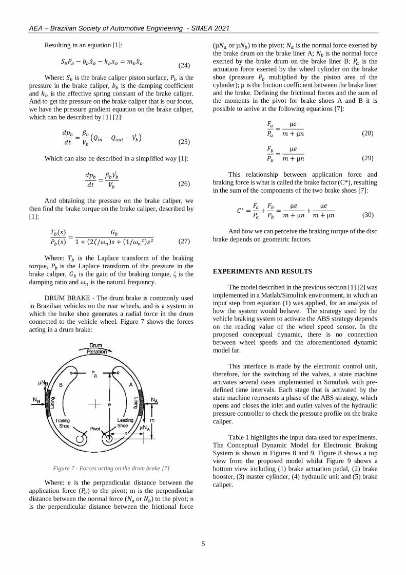
DRUM BRAKE - The drum brake is commonly used
in Brazilian vehicles on the rear wheels, and is a system in
which the brake shoe generates a radial force in the drum
connected to the vehicle wheel. Figure 7 shows the forces
acting in a drum brake:
Figure 7 - Forces acting on the drum brake [7]
Where: e is the perpendicular distance between the
application force (𝑃𝑎) to the pivot; m is the perpendicular
distance between the normal force (𝑁𝑎 or 𝑁𝑏) to the pivot; n
is the perpendicular distance between the frictional force
(µ𝑁𝑎 or µ𝑁𝑏) to the pivot; 𝑁𝑎 is the normal force exerted by
the brake drum on the brake liner A; 𝑁𝑏 is the normal force
exerted by the brake drum on the brake liner B; 𝑃𝑎 is the
actuation force exerted by the wheel cylinder on the brake
shoe (pressure 𝑃𝑏 multiplied by the piston area of the
cylinder); µ is the friction coefficient between the brake liner
and the brake. Defining the frictional forces and the sum of
the moments in the pivot for brake shoes A and B it is
possible to arrive at the following equations [7]:
𝐹𝑎
𝑃𝑎=
µ𝑒
𝑚 + µ𝑛 (28)
𝐹𝑏
𝑃𝑏=
µ𝑒
𝑚 + µ𝑛 (29)
This relationship between application force and
braking force is what is called the brake factor (C*), resulting
in the sum of the components of the two brake shoes [7]:
𝐶∗ =𝐹𝑎
𝑃𝑎+
𝐹𝑏
𝑃𝑏=
µ𝑒
𝑚 + µ𝑛+
µ𝑒
𝑚 + µ𝑛 (30)
And how we can perceive the braking torque of the disc
brake depends on geometric factors.
EXPERIMENTS AND RESULTS
The model described in the previous section [1] [2] was
implemented in a Matlab/Simulink environment, in which an
input step from equation (1) was applied, for an analysis of
how the system would behave. The strategy used by the
vehicle braking system to activate the ABS strategy depends
on the reading value of the wheel speed sensor. In the
proposed conceptual dynamic, there is no connection
between wheel speeds and the aforementioned dynamic
model far.
This interface is made by the electronic control unit,
therefore, for the switching of the valves, a state machine
activates several cases implemented in Simulink with pre-
defined time intervals. Each stage that is activated by the
state machine represents a phase of the ABS strategy, which
opens and closes the inlet and outlet valves of the hydraulic
pressure controller to check the pressure profile on the brake
caliper.
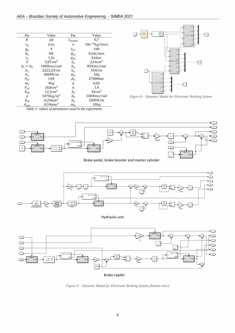
Table 1 highlights the input data used for experiments.
The Conceptual Dynamic Model for Electronic Braking
System is shown in Figures 8 and 9. Figure 8 shows a top
view from the proposed model whilst Figure 9 shows a
bottom view including (1) brake actuation pedal, (2) brake
booster, (3) master cylinder, (4) hydraulic unit and (5) brake
caliper.
AEA – Brazilian Society of Automotive Engineering - SIMEA 2021
6
Par Value Par Value
𝐾 2𝑁 𝐶𝑞,𝑚𝑎𝑥 0,7
𝜏𝑝 0,5𝑠 𝑣 10𝑒−6𝑘𝑔/(𝑚𝑠)
𝑔𝑝 4 𝜆𝑐𝑟 100
𝐾𝑎 8𝑁 𝑄𝑠𝑠 0,26𝑙/𝑚𝑖𝑛
𝜏𝑎 1,5𝑠 𝑝𝑡ℎ 0,6𝑏𝑎𝑟
𝑆 5,07𝑐𝑚2 𝑆𝑎 2,54𝑐𝑚2
𝑏1 = 𝑏2 100𝑁𝑚𝑠/𝑟𝑎𝑑 𝑏𝑎 85𝑁𝑚𝑠/𝑟𝑎𝑑
𝑘1 2222,2𝑁/𝑚 𝑘𝑎 35𝑁/𝑚
𝑘2 4000𝑁/𝑚 𝑚𝑎 10𝑔
𝐹𝑓2 14𝑁 𝛽𝑛 27000𝑏𝑎𝑟
𝑚2 40𝑔 𝛼 0,02
𝑉10 18,8𝑐𝑚3 𝑛 1,4
𝑉20 12,5𝑐𝑚3 𝑆𝑏 45𝑐𝑚2
𝜌 1070𝑘𝑔/𝑚3 𝑏𝑏 100𝑁𝑚𝑠/𝑟𝑎𝑑
𝐴𝑖𝑛 0,29𝑚𝑚2 𝑘𝑏 2000𝑁/𝑚
𝐴𝑜𝑢𝑡 0,59𝑚𝑚2 𝑚𝑏 100𝑔
Table 1: values of parameters used in the experiment.
Figure 8 – Dynamic Model for Electronic Braking System
Figure 9 – Dynamic Model for Electronic Braking System (bottom view)
Brake pedal, brake booster and master cylinder
Hydraulic unit
Brake capiler

AEA – Brazilian Society of Automotive Engineering - SIMEA 2021
7
It is possible to verify a gain of 32.5 times the
application of force in the brake pedal, by the first force
multipliers, pedal and brake booster in Figure 10:
Figure 10 - Input force and mechanical gains
The strength gain of the booster is the force value that
reaches the master cylinder and then starts to generate the
braking pressure. With that, the four ABS stages were
simulated as previously described, and the result obtained
can be seen in Figure 11:
Figure 11 - Pressure profile on the brake caliper after ABS steps x
Applied Force
PHASE 1 (PH 1) - In this stage, we have the nominal
braking, following the Pascal principle for pressure in a
hydrostatic system. Here the valves are in their initial
positions allowing the fluid to flow freely over the ducts. Up
to the 3 seconds (see Figure 12), it is simulating the pressure
on the brake caliper according to the driver's performance.
PHASE 2 (PH 2) - It is the pressure retention stage, in
which the ABS detects the imminence of a wheel lock and
closes the inlet valve referring to that wheel, keeping the
pressure constant. This step occurs due to the speed of the
wheel, but as in the physical model of the brake we have no
way to detect this phenomenon, all steps were done through
predetermined time intervals. Then we have the brake caliper
pressure at this stage:
Between the 3 and 4 seconds of Figure 11, the pressure
in the brake caliper was kept constant, simulating the
pressure locking step on the wheel.
PHASE 3 (PH 3) - This is the phase of emptying the
brake caliper to relieve brake pressure, causing the wheel to
turn again. The system opens the outlet valve and starts the
electric motor to start the pump so that the oil is thrown back
into the circuit. In the simulation seen in Figure 11, this stage
was divided into 2 parts, with an interval of 4 to 5 seconds,
only the outlet valve was opened, so that the accumulator
absorbs the pressure of the hydraulic fluid that was in the
brake caliper, and between moments 5 and 7 seconds, the
electric motor was started so that the hydraulic pump
removes the brake fluid that was in the brake caliper.
PHASE 4 (PH 4) - Finally, this is the phase of filling
the brake caliper again, in which the valves return to their
initial state and the brake caliper is filled with hydraulic fluid
again as shown in Figure 11. As we can see, in this stage the
brake caliper filling is much more abrupt than at the
beginning of the simulation, because in that instant of 7
seconds when the inlet valve is opened again, the system is
already at its maximum pressure, whereas in the instant
initial simulation the pressure was gradual.
To verify the efficiency of this braking system, a
longitudinal model built by [8] will be used, in which the
vehicle's acceleration and gear values are chosen, and the
model returns the vehicle's speed. The pressure profile
shown in this article was included in the test at key points,
and the result compared to validate the conceptual braking
model presented in this article. As we can see in figure 12.
The first graph shows the vehicle speed in the
simulation with the braking system acting (red) and the
vehicle speed without the braking system acting (blue).
While the second graph shows three braking situations.
In which the first situation occurs for a time of 30 seconds
with the total braking capacity used, the second situation
occurs for a time of 20 seconds with 50% of the braking
capacity, and in the third situation we have a performance of
20 seconds with total braking capacity.
It is possible to verify that in the three situations the
brake system is able to reduce the vehicle speed to zero, in
the first case it reduces from 140km/h to 0km/h and in the
second and third it reduces it around 40km/h until it stops
completely vehicle.

AEA – Brazilian Society of Automotive Engineering - SIMEA 2021
8
Figure 12 - Comparative test with and without braking action.
Then, we analyze only the first braking situation and
the comparison of the speed curves. Being able to identify in
the braking graph the four ABS steps explained previously
along with the vehicle's speed drop:
Figure 13 - Speed comparison during braking.
Analyzing the result obtained in figure 13, it is possible
to verify a great similarity with what happens with the
pressure on the brake caliper in a real situation of vehicle
braking, as seen in the Figure 14.
Figure 14 - ABS performance in pressure reduction [9]
In this test, the rotation of the wheel was monitored, so
that the ABS can enter into action, showing the pressure in
the brake caliper in phases 1, 2, and 3 of ABS operation,
which has the same characteristic profile of the experiment
carried out in this work.
CONCLUSIONS
The objective of this work was to present a conceptual
nonlinear Dynamic Model of an automotive brake system
and to simulate it in a computational environment. In this it
was possible to verify the model of the brake system in
computational experiments acting on a simplified
longitudinal dynamic model of a vehicle, where it was
possible to verify the speed drop when the system was
activated.

AEA – Brazilian Society of Automotive Engineering - SIMEA 2021
9
The results achieved will be important for the design
and assembly of an electronic braking system that will be
applied to a platform vehicle for the development of ADAS
functions, which will be implemented from a Fiat Strada
model vehicle. Initially, a platform will be built consisting of
the original braking system and an ABS / ESC module in
which a "black box" model of the system will be obtained.
This will allow, together with vehicle dynamics software, to
develop braking control at the simulation level.
Subsequently, the brake caliper pressure will be obtained
from the physical brake platform and transported to a
LABCAR platform where the same vehicle dynamics
software will be installed, responding in real time, thus
constituting Hardware in the Loop (HiL). This HiL will
allow a first calibration and validation of the control unit.
Finally, the system will be transported to the vehicle, for a
final calibration and validation phase.
BIBLIOGRAPHY
[1] M.-c. Wu e M.-c. Shih, “Simulated and experimental
study of hydraulic anti-lock braking system using
sliding-mode PWM control,” Mechatronics, 2003.
[2] A. Tota, E. Galvagno, M. Velardocchia e A. Vigliani,
“Passenger Car Active Braking System model and
experimental validation (Part I),” JOURNAL OF
MECHANICAL ENGINEERING SCIENCE, 16
fevereiro 2019.
[3] J. Zhang, C. Lv, X. Yue, Y. Li e Y. Yuan, “Study on a
linear relationship between limited pressure difference
and coil current of onoff valve and its influential
factors,” ISA Transactions, 2014.
[4] C. Lv, H. Wang e D. Cao, “High-Precision Hydraulic
Pressure Control Based on Linear Pressure-Drop
Modulation in Valve Critical Equilibrium State,”
IEEE Transactions on Industrial Eletronics, 10
outubro 2017.
[5] “Let's Diskuss,” 18 outubro 2018. [Online]. Available:
https://www.letsdiskuss.com/explain-about-abs-
system. [Acesso em 26 agosto 2020].
[6] “MathWorks,” [Online]. Available:
https://la.mathworks.com/help/physmod/sdl/ref/discbr
ake.html. [Acesso em 26 agosto 2020].
[7] M. B. Müller, Proposta de uma metodologia para
desenvolvimento de novo fornecedor de freios
traseiros a tambor para veículos já em produção, São
Paulo: Universidade de São Paulo, 2009.
[8] E. L. S. Teixeira, J. V. A. Guimarães, L. A. A. M. e
M. M. D. Santos, “LOW-COST PLATFORM FOR
AUTOMOBILE SOFTWARE DEVELOPMENT,”
SAE, p. 10, 2020.
[9] “Notícias da Oficina,” VW Das Auto, 2020. [Online].
Available:
http://www.noticiasdaoficinavw.com.br/v2/2013/02/si
stema-antibloqueio-abs-funcionamento-e-sistema-
eletrico/. [Acesso em 26 agosto 2020].
[10
]
S. Sheikholeslam e C. A. Desoer, “Longitudinal
Control Of A Platoon Of Vehicles. III, Nonlinear
Model,” UC Berkeley, abril 1990.
[11
]
D. Godbole e J. Lygeros, “Longitudinal Control of the
Lead Car of a Platoon,” PATH TECHNICAL
MEMORANDUM 93-7, novembro 1993.
[12
]
D. L. Luu e C. Lupu, “Dynamics model and Design
for Adaptive Cruise Control Vehicles,” 22nd
International Conference on Control Systems and
Computer Science (CSCS), 2019.