A COMPUTABLE GENERAL EQUILIBRIUM

ANALYSIS OF CURRENT CLIMATE CHANGE POLICY IN THE UNITED STATES

by

Jodie L. Capling B.Sc., McGill University, 2005

RESEARCH PROJECT SUBMITTED IN PARTIAL FULFILLMENT OF THE REQUIREMENTS FOR THE DEGREE OF

MASTER OF RESOURCE MANAGEMENT

In the School of Resource and Environmental Management

© Jodie L. Capling 2010

SIMON FRASER UNIVERSITY

Spring 2010

All rights reserved. However, in accordance with the Copyright Act of Canada, this work may be reproduced, without authorization, under the conditions for Fair Dealing. Therefore, limited reproduction of this work for the purposes of private

study, research, criticism, review and news reporting is likely to be in accordance with the law, particularly if cited appropriately.

ii

APPROVAL

Name: Jodie L. Capling

Degree: Master of Resource Management

Title of Thesis: A Computable General Equilibrium Analysis of

Current Climate Change Policy in the United States

Project No.: 491

Examining Committee:

Chair: Caroline Lee Master of Resource Management Candidate

________________________________________

Mark Jaccard

Senior Supervisor Professor, School of Resource and Environmental Management Simon Fraser University

________________________________________

Nic Rivers

Supervisor Ph.D. Candidate, School of Resource and Environmental Management Simon Fraser University

Date Defended/Approved: ________________________________________

iii

ABSTRACT

In this research I develop a static computable general equilibrium model of

the global economy and apply the model to analyze greenhouse gas emission

reduction policy. The model is comprised of two regions, the US and ROW (Rest

of World), and I use it to simulate policy from 2010 to 2050 in 10 year intervals. I

focus on analyzing cap-and-trade systems currently relevant in the US. I found

that reducing emissions with a cap-and-trade system would have moderate costs

and small negative impacts on the US GDP and consumer welfare. I also found

that output-based allocation of revenue to industry could slightly increase the

price of emission permits and that linking a US cap-and-trade system to

international systems could reduce the price of emission permits in the US. In my

analysis carbon capture and storage has an important role in emissions

mitigation.

Keywords: Climate change policy; Computable general equilibrium model; Energy-economy modelling; US cap-and-trade systems

iv

ACKNOWLEDGEMENTS

I would like to thank Mark Jaccard for his guidance through this project

and for his boundless enthusiasm. A huge thanks goes to Nic Rivers, who always

provided guidance and made time to help out with the technical details and

problem solving involved with CGE modelling. Nic’s work in CGE modelling had a

huge influence on the model structure and terminology I used in this project. I

would like to thank Caroline Lee for collaborating with me in building the model

and for making this whole project way more fun. I would also like to thank Jotham

Peters for his modelling expertise, the rest of EMRG for all the help and support

along the way and Noory Meghji for being our ‘office mom’ and keeping EMRG

running smoothly.

Finally, I would like to thank Ben Smith and Lynn and Steve Capling for all

their love and support.

I am grateful for the funding I received from the Natural Sciences and

Engineering Research Council of Canada (NSERC) and the Canadian Industrial

Energy End-Use Data and Analysis Centre (CIEEDAC), as well as the graduate

fellowship I received from Simon Fraser University.

v

TABLE OF CONTENTS

Approval...........................................................................................................................ii Abstract...........................................................................................................................iii Acknowledgements .........................................................................................................iv

Table of Contents............................................................................................................ v

List of Figures ................................................................................................................vii List of Tables ..................................................................................................................ix

Glossary.......................................................................................................................... x

1: Introduction............................................................................................................... 1

1.1 International Response to Climate Change ............................................................. 2

1.2 Situation in the United States .................................................................................. 4

1.3 Energy-Economy Modelling .................................................................................... 5

1.4 VERITAS-US a CGE Informed by CIMS ................................................................. 9

1.5 Research Objectives and Questions ..................................................................... 10

1.6 Report Outline....................................................................................................... 12

2: Methods................................................................................................................... 13

2.1 Computable General Equilibrium Models .............................................................. 13

2.2 Modelling System.................................................................................................. 17

2.3 VERITAS-US Model.............................................................................................. 17

2.3.1 Sectoral Production ................................................................................... 23

2.3.2 International Trade Blocks ......................................................................... 30

2.3.3 Carbon Emission Permits .......................................................................... 32

2.3.4 Consumption Blocks.................................................................................. 33

2.3.5 Additional Features ................................................................................... 35

2.4 Parameter and Data Sources................................................................................ 39

2.4.1 Social Accounting Matrix Data................................................................... 39

2.4.2 Fossil Fuel Forecasts ................................................................................ 41

2.4.3 Elasticities of Substitution.......................................................................... 42

2.5 Analysis ................................................................................................................ 48

2.5.1 Policy Simulation Cases and Assumptions ................................................ 48

3: Simulation Results.................................................................................................. 54

3.1 Business-as-Usual Simulation Results.................................................................. 54

3.2 Marginal Abatement Cost Curves ......................................................................... 56

3.3 Policy Simulation Results...................................................................................... 58

3.4 Sensitivity Analysis ............................................................................................... 68

4: Discussion............................................................................................................... 74

4.1 Comparison with Other Models ............................................................................. 74

vi

4.1.1 Business-as-Usual CO2 Emissions and GDP ............................................ 74

4.1.2 Emission Reduction Policies...................................................................... 77

4.2 Alternative Policy Cases ....................................................................................... 85

4.3 Uncertainty............................................................................................................ 91

4.4 Challenges of Static CGE Modelling ..................................................................... 93

5: Conclusions ............................................................................................................ 95

5.1 Summary of Research Findings ............................................................................ 95

5.2 Future Model Development and Research ............................................................ 99

Appendices ............................................................................................................... 102

Appendix A: VERITAS-US Code in GAMS/MPSGE .................................................... 103

Appendix B: Set j - Sectors in VERITAS-US ............................................................... 112

Appendix C: Sector Specific Elasticities of Substitution for the US and ROW.............. 113

Reference List ........................................................................................................... 114

vii

LIST OF FIGURES

Figure 2.1 Schematic of a Basic Economy ................................................................. 14

Figure 2.2 Regional Structure of VERITAS-US........................................................... 20

Figure 2.3 Nesting Structure for Elasticities in Y Production Block ............................. 25

Figure 2.4 Nesting Structure for Elasticities in DOMEX Production Block................... 31

Figure 2.5 Nesting Structure for Elasticities in Armington Block ................................. 32

Figure 2.6 Nesting Structure for Elasticities in C Production Block ............................. 34

Figure 3.1 US Business-as-Usual CO2 Emissions ...................................................... 55

Figure 3.2 US Business-as-Usual Gross Domestic Product ....................................... 56

Figure 3.3 US Marginal Abatement Cost Curves ........................................................ 57

Figure 3.4 US CO2 Emission Reduction Pathway for the American Clean Energy and Security Act ........................................................................... 59

Figure 3.5 Global Carbon Permit Price for Core Policy............................................... 60

Figure 3.6 US Equivalent Variation % Decrease for Core Policy ................................ 61

Figure 3.7 US GDP % Decrease for Core Policy ........................................................ 62

Figure 3.8 Carbon Permit Prices With and Without International Permit Trading ........ 63

Figure 3.9 US Equivalent Variation % Decrease With and Without International Permit Trading.......................................................................................... 64

Figure 3.10 US GDP % Decrease With and Without International Permit Trading........ 65

Figure 3.11 US Carbon Permit Price With and Without Output-Based Allocation of Revenue to Industry.............................................................................. 67

Figure 3.12 US Marginal Abatement Curve 2050 - Change in Quantity of CCS Available................................................................................................... 71

Figure 3.13 US Marginal Abatement Curve 2050 - Change in Cost of CCS ................. 72

Figure 4.1 Comparison of Business-as-Usual GDP for the US by VERITAS, MIT-EPPA and ADAGE ............................................................................ 75

Figure 4.2 Comparison of Business-as-Usual CO2 Emissions for the US by VERITAS-US, EIA-NEMS, MIT-EPPA and ADAGE .................................. 77

Figure 4.3 Comparison of Emission Permit Prices for the US by VERITAS-US, MIT-EPPA, ADAGE and MRN-NEEM....................................................... 79

Figure 4.4 Emission Reduction Pathway for the American Clean Energy and Security Act Targets With and Without Offsets ......................................... 83

viii

Figure 4.5 Emissions Permit Price for the American Clean Energy and Security Act Analysis by MIT-EPPA, ADAGE and EIA-NEMS for Full Offset and Limited Offset Cases ......................................................................... 84

ix

LIST OF TABLES

Table 2.1 Set i - Commodities in VERITAS-US .......................................................... 22

Table 2.2 Elasticities of Substitution for Production Functions.................................... 45

Table 2.3 Elasticities of Substitution for Utility Function.............................................. 47

Table 2.4 Elasticities for Import and Export ................................................................ 47

Table 2.5 Carbon Permit Allocation for Core Policy .................................................... 50

Table 3.1 Sensitivity Analysis of ESUB Values for 2050 Simulation ........................... 68

x

GLOSSARY

AEEI Autonomous Energy Efficiency Index

BAU Business-as-Usual

CCS Carbon Capture and Storage

CES Constant Elasticity of Substitution

CGE model Computable General Equilibrium model

CO2 Carbon Dioxide

CO2e Carbon Dioxide Equivalents

EIA Energy Information Administration

ESUB Elasticity of Substitution

EV Equivalent Variation

GAMS General Algebraic Modelling System

GDP Gross Domestic Product

GHG Greenhouse Gas

Gj Gigajoule (109 joules)

GTAP Global Trade Analysis Project

IPCC Intergovernmental Panel on Climate Change

MAC Marginal Abatement Cost

MPSGE Mathematical Programming System for General Equilibrium

Mt Megatonne (106 tonnes)

xi

ppm parts per million

ROW Rest of World

RPP Refined Petroleum Product

SAM Social Accounting Matrix

UNFCCC United Nations Framework Convention on Climate Change

US United States

VERITAS EValuation of Emission Reduction for InTernational Abatement Scenarios

1

1: INTRODUCTION

Climate change is one of the largest challenges that humanity faces today

and it is a challenge of our own making. The Intergovernmental Panel on Climate

Change (IPCC) has found that global atmospheric concentrations of greenhouse

gasses (GHG) have increased since 1750 as a result of human activities and that

levels of GHG now far exceed pre-industrial values (IPCC, 2007a). The IPCC

has also found with very high confidence that the global average net effect of

human activities since 1750 has been one of warming.1

Carbon dioxide (CO2) is the most important anthropogenic GHG and the

atmospheric concentration of CO2 has increased from 280 parts per million (ppm)

in pre-industrial times, to 385 ppm in 2008 (IPCC, 2007a; Keeling et al., 2009).

The current atmospheric concentration of CO2 exceeds the natural range of 180

to 300 ppm seen over the last 650,000 years, as determined from ice cores

(IPCC, 2007a). The main source of increasing CO2 concentrations in the

atmosphere is the combustion of fossil fuels in our energy systems; land use

changes are also important but make a much smaller contribution (IPCC, 2007a;

Karl and Trenberth, 2003).

In this chapter, I briefly describe the international response to

anthropogenic climate change and introduce where the United States is in their 1 The IPCC uses the convention that very high confidence means a 9 out of 10 chance of being

correct.

2

response to this problem. Next, I discuss different types of energy-economy

models and how they contribute to understanding the challenge of addressing

climate change and our options for doing so. I then provide a description and

justification of the type of energy-economy model I use in this research.

Following this, I present my research objectives and questions. An outline of the

rest of this report concludes this chapter.

1.1 International Response to Climate Change

The international response to anthropogenic climate change has been

centred around the United Nations Framework Convention on Climate Change

(UNFCCC). In 1992, many counties joined the UNFCCC, which is an

international treaty that focuses on dealing with the problem of climate change.

The ultimate goal of UNFCCC, as stated in Article 2, is stabilizing greenhouse

gas concentrations at a level that would prevent dangerous anthropogenic

interference with the climate system (United Nations, 1992).

The goal of UNFCCC brings into question what dangerous anthropogenic

interference actually is and what the target should be for stabilizing GHG

concentrations. The fourth IPCC assessment report provides ranges of

temperature increases above pre-industrial values and the corresponding level of

atmospheric carbon dioxide equivalents (CO2e) that might be necessary to stay

within them. CO2e are one way to measure the amount of GHGs in the

atmosphere, taking into account CO2 and GHGs other than CO2. The most

widely supported temperature-limiting goal is to keep global temperature

increase below 2 degrees Celsius from pre-industrial values. Reaching this

3

temperature target is likely to require stabilization at about 450 ppm CO2e (IPCC,

2007a). However, to have an 80% probability that temperature change will be

limited to 2oC, the IPCC estimates that CO2e would need to be stabilized at 378

ppm (IPCC, 2007b). Some groups, particularly small island states, have

proposed that measures should be taken to limit temperature change to less than

1.5oC, which would require even lower levels of stabilized GHG concentrations.

While the IPCC provides a summary of the current scientific information about

climate change, international agreements are shaped by political constraints and

interests of many nations, as well as scientific consensus on climate change.

The Kyoto Protocol is an international treaty that was negotiated under the

UNFCCC. Adopted in December 1997 and entered into force in February 2005, it

sets binding goals for reducing GHG emissions for 37 industrialized countries.

The average targets are to reduce emissions to 5% below 1990 levels for the

period of 2008 to 2012. The Kyoto Protocol acknowledges that industrialized

countries have historically contributed more to the problem of climate change and

that they have a higher financial capacity to pay for mitigation; therefore it puts a

heavier burden on developed nations. One large obstacle that the Protocol faced

was that the United States did not ratify. This means that the two largest emitters

in the world, the US and China, do not have emission reduction targets under the

Kyoto Protocol.

While the Kyoto Protocol is an important step in reaching international

agreements to deal with the issue of climate change, much of the international

focus is now on negotiating a post-Kyoto agreement. There is potential for the

4

US to be a positive influence in these negotiations, since the Obama

administration has made it clear that climate change is a priority. The latest

United Nations climate negotiations resulted in the Copenhagen Accord, which

has recently been finalized. However, the Copenhagen Accord is not legally

binding and essentially summarizes the targets that countries had before the

negotiations began. Whether the targets are met will depend on the domestic

emission reduction policy that individual countries enact.

1.2 Situation in the United States

When it comes to the types of policies that could be used to meet GHG

emission reduction targets, cap-and-trade systems are likely, especially in the

US. In the absence of federal policy, various states and some Canadian

provinces have started designing and implementing cap-and-trade systems to

reduce GHG emissions. Examples include the Western Climate Initiative, which

is working on an international cap-and-trade system in the US and Canada, the

Regional Greenhouse Gas Initiative, which has begun implementing a cap-and-

trade system for power generators in the eastern US, and the Midwestern

Greenhouse Gas Accord, which is working on developing proposals for a cap-

and-trade system in the central US. The European Union also has a cap-and-

trade system in place to reduce GHG emissions. The European Union Emissions

Trading Scheme has been running since 2005 and sets a precedent for the use

of cap-and-trade systems in other regions.

Currently there are two bills that propose cap-and-trade systems for GHGs

before the US Senate. In May of 2009, Representatives Waxman and Markey

5

introduced the American Clean Energy and Security Act of 2009, which is also

known as the Waxman-Markey bill. This bill is a national climate and energy act

that would establish a cap-and-trade system for GHGs and other measures to

address climate change and transition to a low-carbon economy. The House of

Representatives passed the bill on June 26, 2009 and it was received in the

Senate in July 2009. The second bill, the Clean Energy Jobs and American

Power Act, is sponsored by Senators Kerry and Boxer and is also known as the

Kerry-Boxer bill. The focus of this bill is to create clean energy jobs, promote

energy independence, reduce global warming pollution and transition to a clean

energy economy. It was introduced to the US Senate in September of 2009.

Given the elements of both bills, it seems likely that if the US Congress passes

climate change legislation, a key portion will be a cap-and-trade system for

greenhouse gasses.

The timing of policies that influence energy use and energy systems is

central to dealing with climate change. Every year of delay increases the

likelihood that global warming will exceed 2oC above pre-industrial values. To

keep the warming below this level, global emissions need to peak between 2015

and 2020 and then decline rapidly (Allison et al., 2009; IPCC, 2007b). In short,

expedient action and well-crafted policies are necessary to meet the challenge of

reducing GHG emissions and minimizing climate change.

1.3 Energy-Economy Modelling

Energy-economy models are useful in modelling the interactions between

the economy, energy systems and the environment and how technologies affect

6

these interactions (van der Zwaan et al., 2002). These models can be helpful to

policy makers when they are designing policies to meet environmental, social

and economic objectives. In the context of climate change, these models are

often used to estimate how various policies could impact the economy and the

environment, specifically through the amounts of GHGs emitted into our

atmosphere. These models cannot precisely predict the future, but they show

possible trends and scenarios that could occur based on our current situation

and possible choices of policies.

There are traditionally two main approaches to energy-economy

modelling, referred to as bottom-up and top-down. However, the effort to bridge

these two methods is evident in the emergence of hybrid models, which attempt

to capture the best aspects of each and avoid some of their limitations.

Bottom-up Models

Traditional bottom-up models are generally based on rich technological

detail. They estimate how energy use and corresponding environmental impacts

could be affected by changes in energy efficiency, fuel use, emission control

equipment and infrastructure (Bataille et al., 2006). Bottom-up models assume

that a new technology, which provides the same type of service as an existing,

conventional technology, can be substituted directly, only differing in the lower

anticipated financial cost or reduced emissions of the new technology (Jaccard,

2005). This assumption ignores possible intangible costs associated with a new

technology, including: risk of the new technology failing, different quality of

service, and risks associated with long payback investments. It also fails to

7

reflect how consumers or firms behave when faced with decisions about new

technologies. By excluding these costs and behaviours, bottom-up approaches

often underestimate the true cost of low-emission or more efficient technologies,

and thus tend also to underestimate the cost of reducing GHG emissions

(Jaccard, 2005). Bottom-up models also often lack the macro-economic

feedbacks that link changes induced by policies to the structure of the economy

and to the rate or distribution of economic growth (Hourcade et al., 2006).

Top-down Models

Traditional top-down models are based on aggregate representations of

the economy and often use abstract production functions to describe

relationships between sectors, inputs and outputs. They are generally based on

an equilibrium framework that can capture indirect effects from one sector of the

economy to others. The top-down models that are based on full equilibrium are

usually referred to as computable general equilibrium (CGE) models (Löschel,

2002). In these models, technologies are usually represented by aggregate

production functions for each sector of the economy (McFarland et al., 2004) The

lack of technological detail makes top-down models unsuited for analyzing

policies that specifically target technological change, such as subsidies for

specific technologies or standards that mandate minimum market shares of low

emission technologies. The top-down approach is also challenged in portraying

future technological change due to the use of historical data as a basis for many

model parameters (Hourcade et al., 2006).

8

One of the strengths of top-down models is their ability to capture

macroeconomic feedbacks and the changes in the structure of the economy

because of policies. Top-down models are used to analyze market-based

policies, where they use parameters estimated from historic economic data to

simulate the response of the economy to a financial signal. For example, a tax on

GHG emissions is a financial signal, which increases the cost of technologies or

energy forms that produce emissions. The size of the signal needed to attain an

emissions target indicates the implicit challenge of reaching the target, including

intangible costs, such as risk related to new technology and investing in

technologies that may require a long payback period. Thus, top-down cost

estimates of policies are usually higher than bottom-up estimates because they

include the transitional and long run costs of technological change (Jaccard,

2005).

Hybrid Models

In recent years, there has been a trend towards hybrid energy-economy

models, which seek to bridge the gap between top-down and bottom-up. This

has involved bottom-up modellers adding more macro-economic feedbacks and

behavioural realism to their models and top-down modellers adding more

technological explicitness to their models (Hourcade et al., 2006). One example

is the MIT-EPPA model which is a CGE that includes multiple electricity-

producing technologies (Paltsev et al., 2005). Another example of a hybrid model

is CIMS, which is developed by the Energy and Material Research Group of

Simon Fraser University. CIMS is technologically explicit like many bottom-up

9

models, but also captures some of the behavioural and macroeconomic

feedbacks of top-down models. For a description of CIMS see Bataille et al.

(2006) or Murphy et al. (2007).

In this research, I continue along the path of model hybridization, by using

the CIMS model to inform a CGE model. The value of this combination is that it

utilizes the best characteristics of both model types. The CGE model is useful for

tracking the macro-economic impacts and feedbacks that climate change policies

could induce on the economy and the CIMS model is technology-rich and

includes aspects of behavioural realism. By using the CIMS model to inform the

way a CGE model represents technology, it improves the CGE model, but still

allows the modeller to investigate the macro-economic impacts of a policy.

This type of model is especially critical for analyzing climate change policy

in the US because of the key role that this country has in this global issue. As the

second largest GHG emitter on the planet and the largest emitter among the

developed nations, the US must be involved in the solution if we are to

successfully deal with anthropogenic climate change. A model that provides

robust analysis of climate change policy options can help US leaders and

decision makers choose the best policies to meet the challenge of climate

change, while also addressing important economic and social considerations.

1.4 VERITAS-US a CGE Informed by CIMS

My research is based on building a global CGE model to analyze GHG

emission reduction policy with a focus on cap-and-trade policy in the United

10

States. The CGE model that I developed, in conjunction with Caroline Lee, is

called VERITAS (EValuation of Emission Reduction for InTernational Abatement

Scenarios).2 In my research, I focus on evaluation of GHG emission reduction

policy in the US and use a US focused version of the model called VERITAS-US.

One of the strengths of VERITAS-US is that it includes parameters that

are informed by the CIMS model. Thus, it has the macro-economic feedbacks

and behavioural realism of a CGE, combined with aspects of the behavioural

realism and technological detail of CIMS. The parameters that I calculate from

CIMS help address some of the uncertainty in the way a typical CGE model

represents technologies. This combination removes some of the CGE’s

dependence on historical technology data because CIMS details the technology

options that are currently available and those that will potentially be available in

the next few decades. The parameters calculated from CIMS also provide

VERITAS-US with some sector and regionally specific parameters. This

combination is a potential improvement over other CGE models as they often

have the same parameters for all regions and sectors, which are based on expert

opinion or historical data.

1.5 Research Objectives and Questions

Because of the US position as a large GHG emitter and their political

power, their participation in addressing climate change is critical. The Obama

administration has made action on climate change a priority and there are two

2 Also the Roman Goddess of Truth

11

climate change bills before the Senate that would use cap-and-trade systems

with emission permits to reduce GHG emission. Robust analyses of these

climate change policies are important to make sure that they will meet

environmental, economic and social objectives. In designing and passing a

climate change bill there are many important issues. One such issue is that of

international emissions permit trading and how a US GHG emission reduction

policy could be linked to emission reduction efforts internationally. Another

important issue is how emission permits or revenue from auctioning of the

permits might be allocated and how this could impact the US. The objectives and

questions for this research project are a response to these important issues in

the current situation and the necessity for analyses of climate change policy

options for the US.

Objectives:

• To build a global energy-economy model able to analyze

climate change policy, with a focus on the United States (using

a CGE framework enhanced with information from CIMS),

• To use the model to analyze climate change policy that is

currently relevant to American and international situations.

Questions:

• What are the potential economic and environmental impacts of

currently proposed US climate policy?

12

• What are the potential effects of trading carbon permits internationally

versus the option of the US acting alone without international permit

trading?

• What are the potential impacts of revenue recycling or permit allocation

within the US?

• How robust is the model to different values for elasticities of

substitution and the assumptions made regarding carbon capture and

storage costs and capacity?

1.6 Report Outline

Chapter 2 describes the methods I use, including the modelling system for

building VERITAS-US, the model structure and the policy cases to answer my

research questions. Chapter 3 contains results from the runs of the model and

the policy simulations. Chapter 4 provides a discussion of the results and a

comparison of my results to those from other models that are used for similar

types of policy analysis. Conclusions arising from this project and some

recommendations for future research are presented in Chapter 5.

13

2: METHODS

In this chapter, Sections 2.1 and 2.2 describe CGE models in general and

the modelling systems I used for the project. An overview and details on the

VERITAS-US model are provided in Section 2.3. In Section 2.4, I describe the

data sources and treatment that I used in building the model. Section 2.5

contains a description of the policy scenarios that I analyze in this project.

2.1 Computable General Equilibrium Models

VERITAS-US is a computable general equilibrium (CGE) model of the

global economy. In this context, computable indicates that a solution for the

model is calculated and general equilibrium denotes that all markets in the

economy are in equilibrium when a solution is found.

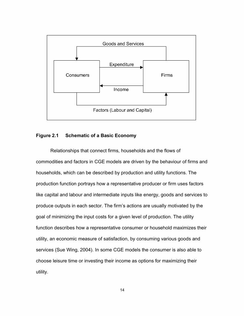
CGE models are based on the idea of a circular flow of commodities

(goods and services) and factors (labour and capital) between agents (firms and

households) in the economy. Figure 2.1 shows a very basic economy where

consumers rent their time, as labour, and their investments, as capital, to firms in

exchange for income and firms in turn, sell goods and services to consumers. In

some CGE models, there is also a government, which transfers wealth by

collecting taxes and providing services or giving subsidies to households and

firms (Paltsev et al., 2005; Sue Wing, 2004).

14

Figure 2.1 Schematic of a Basic Economy

Relationships that connect firms, households and the flows of

commodities and factors in CGE models are driven by the behaviour of firms and

households, which can be described by production and utility functions. The

production function portrays how a representative producer or firm uses factors

like capital and labour and intermediate inputs like energy, goods and services to

produce outputs in each sector. The firm’s actions are usually motivated by the

goal of minimizing the input costs for a given level of production. The utility

function describes how a representative consumer or household maximizes their

utility, an economic measure of satisfaction, by consuming various goods and

services (Sue Wing, 2004). In some CGE models the consumer is also able to

choose leisure time or investing their income as options for maximizing their

utility.

15

The ability to make tradeoffs between inputs in production and utility

functions is described by elasticities of substitution (ESUBs). These parameters

are very important in CGE models because they regulate how the technologies

and preferences of firms and consumers may change, resulting in a different mix

of inputs. For example, if a policy that increases the cost of natural gas is

imposed, the ESUBs determine how easily a firm or consumer can shift away

from natural gas use towards the use of a less expensive fuel. Therefore, these

ESUB values have a large impact on how costly a policy is projected to be

(Paltsev et al., 2005).

In this project, I use nested constant elasticity of substitution (CES)

functions to represent the activities of production and consumption by firms and

households. Nested refers to the hierarchical structure that relates the different

inputs and their associated ESUBs. I give examples of the nested structures in

Section 2.3. Constant refers to the fact that the ESUB values remain constant

even if the proportions of inputs in a function change.

For a CGE model of a closed economy to be in equilibrium there are three

conditions that must be observed: market clearance, income balance and zero

profit (Sue Wing, 2004). Market clearance requires that goods produced must

equal goods demanded. To meet the condition of income balance, the value of

payments households receive from firms for the use of their labour and capital

factors must equal the value of commodity purchases by households. In other

words, the consumer must expend all income, although some models allow

consumers to save or invest part of their income. The final condition of zero profit

16

is met when the total value of outputs produced is equal to the sum of the value

of factors and intermediate inputs used by producers.

Social accounting matrices (SAMs) are central in CGE modelling as they

provide data and partially determine model structure. SAMs are created from

multiple data sources, including national and product accounting data and input-

output tables. They show a static picture of economic transactions in a country or

region for a given time period (Pyatt and Round, 1985). The level of aggregation

of the data in the SAMs determines part of the CGE’s structure. For example,

consider a CGE model based on a SAM that is aggregated so the economy is

represented by firms and households only and the firms are lumped into two

sectors: industry and services. This CGE would have only two sectors, industry

and services, and households would be the only final consumer.

An important parameter in energy-focused CGE models is the

autonomous energy efficiency index (AEEI). This parameter represents the

decoupling of energy use and economic growth from energy price changes; a

larger AEEI parameter indicates that the economy is becoming more efficient at

using energy relatively rapidly (Bataille et al., 2006; Löschel, 2002). This

parameter is a function of both capital stock turnover and technology

improvements, independent of energy price changes.

In the field of CGE modelling, there are two sub-types called static and

dynamic models. Static models are more simplistic and represent a snapshot of a

single time period. Dynamic models have a time component and therefore run

over multiple time periods. In a dynamic model, the previous time periods can

17

affect the future ones through multiple factors like prior energy prices, prior time

periods’ investment levels and capital stock built in prior time periods. VERITAS-

US is a static CGE model.

2.2 Modelling System

To build VERITAS-US, I used the General Algebraic Modelling System

(GAMS) in conjunction with the Mathematical Programming System for General

Equilibrium (MPSGE). Developed by Meeraus et al. (1988), GAMS has a variety

of routines that can be used to solve linear, non-linear and mixed integer

mathematical models and programming problems. A feature of GAMS is that one

can build a model without reference to a specific data set, so the same model

can be used with multiple data sets of the same format.

While GAMS can be used for a variety of problems, MPSGE, developed

by Rutherford (1987, 1997), is specifically designed for economic equilibrium

models. MPSGE provides a shorthand way to represent the complicated

mathematics that general equilibrium models are based on. It uses nested

constant elasticity of substitution production and utility functions. Versions of

GAMS with MPSGE embedded have been available since 1993.

2.3 VERITAS-US Model

VERITAS-US is a multi-region, static CGE model, which is comprised of

two regions, the United States and Rest Of World (ROW). As a static model,

each run of VERITAS-US corresponds to only one time period, so to simulate

polices out to 2050, I run the model separately for 2004, 2010, 2020, 2030, 2040

18

and 2050. The model is a representation of the economy of each region, where

factors (capital, labour, land and natural resources) are endowed to households

and firms use intermediate inputs and factors to produce goods and services,

which are in turn demanded by the final consumer. This final consumer

represents both households and government functions. The model also includes

exports and imports and tracks bilateral trade. VERITAS-US is able to account

for CO2 emissions based on the combustion of fossil fuels. While I could use the

model to analyze carbon tax policies, I have chosen to focus on policies that use

a cap-and-trade system with emission permits.

The way the model works is driven by two key assumptions about how

firms, or producers, and consumers act. There are two parts to the assumption

regarding firms. First, they produce with constant-returns-to-scale, i.e. if total

inputs increase or decrease, the output changes proportionally. Second, the firms

choose inputs to minimize costs for a given level of production. The assumption

regarding the actions of consumers is that they maximize their utility, or

satisfaction, by maximizing their consumption for a given amount of income.

Equilibrium is reached in the model when the three equilibrium constraints

(market clearance, income balance and zero profit) are obeyed and both the

firms and consumers have achieved their respective cost-minimizing and utility-

maximizing goals.

To use VERITAS-US to simulate a policy, I first have the model perform a

business-as-usual run. Next, the model is pushed out of equilibrium by applying a

policy for reducing GHG emissions. The policies that I simulate put a cap on the

19

amount of carbon emissions allowed in a region and use emission permits to

allow individuals or firms to produce emissions, which essentially adds a cost to

emitting carbon because of the value of the permits. The model must then reach

a new equilibrium taking into account the added costs associated with emitting

carbon. I compare this new equilibrium state to the original business-as-usual run

to determine the potential impacts of the policy.

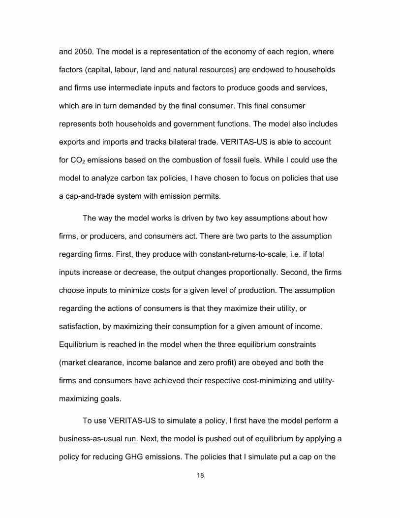
The schematic of the overall structure of VERITAS-US (Figure 2.2) shows

how each regional economy is represented. Each box, called a ‘production

block,’ represents a transformation activity, where inputs are transformed into

outputs as goods and factors flow through the economy. These boxes also

correspond to blocks of code in the MSPGE section of my model. The box

containing Y, X and Ya represents the activity of sectoral production and uses

factors and intermediate goods to produce domestic commodities, while

minimizing the cost of inputs. The DOMEX box is for transformation of these

domestic goods into goods for export and goods for domestic consumption. This

is based on the assumption that goods for export and goods for domestic

consumption are not perfect substitutes. The IMP box, at the top of the figure,

imports goods from other regions. The A box is the Armington aggregator, which

amalgamates imported and domestic goods into Armington goods for domestic

consumption. This is based on the assumption that goods produced in different

places are not perfect substitutes. The Armington goods are used by the sectors

as intermediate goods and by the consumer for meeting final demand. The

CARB production block allocates emission permits to carbon-emitting fuels.

20

Figure 2.2 Regional Structure of VERITAS-US

21

The C block, in Figure 2.2, aggregates all the consumable goods and the

CON block represents consumer demand and factors endowed to them. The

consumer demand is based on the maximization of utility, or satisfaction, for a

given level of income. The GAMS/MPSGE code for VERITAS-US is in Appendix

A.

In building VERITAS-US, I used sets to organize the data as shown in

Figure 2.2 in the bracketed subscripts. I included the subscripts to aid those

readers who wish to understand the model code in Appendix A. The sets consist

of: regions, r ; commodities, i ; sectors, j ; factors, f ; and steps in the carbon

capture and storage option, s. In the figure, the subscripts ‘nce’ and ‘fe’ are also

used, both of which are subsets of the commodity set i. They refer to non-carbon

emitting (nce) commodities and fuels that emit (fe). The subscript rr is an alias for

r and is used when multiple regions are defined, for example, with the exports

PX(r,rr,i), r refers to the region the exports are coming from and rr refers to the

regions that they are going to.

I chose the two regions, US and ROW, so VERITAS-US includes an

approximation of the US interacting with the rest of the globe. This allows me to

analyze US policy while having the rest of the world enacting policy as well.

Having the ROW region is also important when modelling the US because the

US is a large open economy; i.e., it is large enough that changes in US

consumption can affect the global price of commodities. The two regions allow

for more realism in global trade as commodity and energy prices change.

22

The set of commodities, i, tracked by VERITAS-US is shown in Table 2.1.

In this model, each sector only produces one type of commodity, thus there is a

sector, j, that corresponds to each of the commodities in the table below. A

detailed description of the activities of each sector is in Appendix B.

Table 2.1 Set i - Commodities in VERITAS-US

OIL Crude Oil MET Metal Industrial Goods

ELEC Electricity NMET Non-Metal Industrial Goods

GAS Natural Gas OMAN Other Manufactured Goods

COAL Coal TRAN Transportation

RPP Refined Petroleum Products

ROE Other Goods and Services in Rest of Economy

The model has four types of factors: labour, capital, land and natural

resources, which are divided into two subsets, sluggish and mobile. Sluggish, or

sector-specific, factors include land, natural resources and fixed capital, which

are only used by the sectors they are originally assigned to in the business-as-

usual data. I made this distinction because, for example, land used for coal

mining is not easily transferred to agricultural use. Mobile factors are labour and

flexible capital, which can be used in any of the sectors.

In the next four sections, I describe the function of each ‘production block’

in the schematic of VERITAS-US, Figure 2.2.

23

2.3.1 Sectoral Production

Sectoral production of commodities occurs in the three production blocks

Y, X and Ya, and for the most part they are modeled with very similar structure.

The Y and X production blocks represent conventional sectoral production; the

difference being that Y uses flexible capital as an input and X uses only fixed

capital. Flexible capital in the Y production block is open to use by any of the

sectors and represents investment in new production technologies. The fixed

capital in X must stay in the sector it is assigned to, as it corresponds to installed

or built capital. For example, a power plant built to produce electricity cannot be

used by the manufacturing sector to process beverages. The Ya production block

corresponds to the alternative electricity-producing sector with production

technologies that use carbon capture and storage (CCS). This alternative

electricity sector is optional and is only used when policies make it economically

advantageous to acquire CCS technology instead of conventional combustion

technologies that require expensive emissions permits. It uses flexible capital as

these CCS technologies would not be installed in the business-as-usual run

because of the absence of policy that puts a price on emissions.

The proportion of total capital available to the Y, X and Ya production

blocks changes for different time periods. The total amount of capital that is

either flexible or fixed is based on the annual capital depreciation rate of 4% per

year (Center for Global Trade Analysis, 2001). In the first few time periods, most

of the capital is fixed and used only in the X block. In later decades, as fixed

capital depreciates and is replaced by flexible capital, a higher proportion of the

24

capital available in the model is flexible and can be used in the Y or Ya blocks.

This distinction between fixed and flexible capital allows for more structural

change of the modeled economy in later decades. Models that have this ability to

differentiate between fixed and flexible capital are often referred to as “putty-clay”

models.

Firms, which are represented by the Y production block, use the inputs of

factors and intermediate goods and services to produce output. Figure 2.3 shows

the nesting structure of the constant elasticity of substitution (CES) production

function with all the inputs at the ends of branches and the sectoral production

output at the top of the figure. The inputs to Y include: factors of land, natural

resources, flexible capital and labour; coal, natural gas and refined petroleum

products (RPP) with associated carbon permits; and non-carbon emitting goods

and services like non-energy commodities and electricity. The output of this block

is the sectoral production of the commodity produced by each individual sector,

for example, natural gas is the output of the GAS sector.

25

Figure 2.3 Nesting Structure for Elasticities in Y Production Block

In Figure 2.3, the elasticities of substitution (ESUBs), which embody the

ability of available technologies to use various proportions of inputs, are

represented by the symbol, !, with subscript labels. Starting at the top of the

figure, the ESUB between non-energy commodities and the combined bundle of

energy commodities and factors is !S. !VAE is the ESUB between factors and

energy commodities. In the left branch of the figure, !VA is the ESUB between

sluggish and mobile factors. !SLUG is the ESUB between land and natural

resources and !MOB is the ESUB between flexible capital and labour. The right

branch of the figure shows the energy inputs, where !E is the ESUB between

26

electricity and fossil fuels. !FUEL is the ESUB between coal and liquid fossil fuels

and !LQD is the ESUB between natural gas and RPP.

The conventional production in the X block is very similar to that in the Y

block with a couple of differences. The first is that X uses fixed capital instead of

flexible capital as an input. The second difference is that the ESUB values in X

are assumed to be zero because the X block represents installed capital, which I

assume cannot alter the inputs it requires. The output that the firms represented

by the X block produce is the same as the sectoral production output by the firms

represented by the Y block.

The alternative electricity production sector, Ya, allows for the optional use

of carbon capture and storage (CCS) in the electricity sector. By allowing for

CCS in Ya, approximately 85% of carbon emissions from the sector’s fuel use

are captured and stored and I include this in the model by making the Ya block

generate carbon permits for all captured carbon emissions. This alternative

electricity sector allows the model to use CCS technologies if a policy makes the

cost of emitting high enough that they become economically feasible. This sector

represents CCS technologies, which are divided into three steps that have limited

amounts of available capacity. The first two steps represent lower and higher

cost estimates for CCS technologies that use fossil fuels and the third step

represents CCS using biomass as feedstock. As a policy increases the cost of

emitting, the model will shift toward the allowed capacity to produce electricity

with CCS, starting with the cheapest step and then moving to the more costly

steps.

27

This alternative electricity production block, Ya, generally has the same

input and output requirements as conventional electricity production, Y, with a

couple of additional requirements. These are PQ(r,j,s), which is the quantity of

CCS allowed and land resources, which are required by the biomass step to

simulate the land supply constraints of using biomass feedstock. While the

alternative electricity sector requires most of the same type of inputs as the

conventional electricity sector, it requires more capital and fuel than the

conventional sector. The additional output is PCARB(r), which is the carbon

permits for the stored emissions and the other output of Ya is electricity, which is

the same output as the conventional electricity-producing sector. The alternative

electricity sector produces electricity and carbon permits in fixed proportions.

The situation with the ESUBs in the alternative electricity-producing sector

is different from the conventional electricity production sectors. The structure of

the nested elasticities is similar to that of the conventional Y sectors (Figure 2.3)

but most of the ESUBs in Ya are set to zero. The exceptions are fossil fuel

related ESUBs which have the same values as in Y. These ESUBs are

necessary because Ya represents technology steps involving CCS; however, the

first two steps are amalgamations of multiple types of electricity production plants

that use coal, natural gas or refined petroleum products to produce electricity

with CCS. The initial proportions for the use of each type of fuel are the same as

in the business-as-usual data, but as prices change in the policy runs, the

ESUBs allow for shifting between fuels used in the technologies in Ya. The

ESUBs between energy and factors and between capital and labour are set to

28

zero because I assume the proportions of capital required in the CCS

technologies are fixed.

The alternative electricity-producing sector, Ya, requires technical data,

such as the required increase in capital and fuel and the amount of required

biomass, to represent electricity production using CCS technologies. In the

model, the percent increase of capital required by the CCS technologies ranges

from 42% to 80% and the percent increase of required fossil fuel ranges from

17% to 30% in the first two CCS steps. These ranges for capital and fuel use

mark-ups are based on high and low estimates of CCS technology costs from the

IPCC (IPCC, 2005). The mark-up of capital for biomass CCS is based on the

estimate that the cost will be double that of conventional CCS (IEA, 2006; Reilly

and Paltsev, 2007). I used land as a proxy for biomass feedstock because

VERITAS-US does not track biomass. Reilly and Paltsev (2007) estimated that

land makes up a proportion of 19% of the total dollar value of inputs required for

biomass CCS and I used this estimation in my approximation of biomass CCS

technologies.

The amount of emissions that are captured is also an important part of

representing the CCS technologies. I assume that 85% of carbon emissions from

the fossil fuels combusted are captured (IPCC, 2005). The amount of emissions

captured by the biomass CCS step is more complicated as land is used as an

approximation for biomass feedstock. The amount of carbon emissions captured

by biomass CCS is based on tonnes CO2 stored per dollar of electricity output. I

used the value of 0.0007 Mt per dollar of electricity output, which is an estimate

29

from Rhodes and Keith (2005) where they assume that the production, harvest

and transport of the biomass feedstock does not produce emissions.

The capacity of the alternative electricity-producing sector is also

important. The amount of CCS electricity that the model can produce in 2020 and

2030 is set equal to the business-as-usual (BAU) electricity production, with the

capacity equally divided between the three steps. While the capacity is available,

the model only uses the CCS steps if they are economically feasible. In 2040 and

2050, the available capacity of the alternative electricity sector, Ya, is set to

120% of the BAU electricity use to allow for fuel switching to electricity in

transport, buildings and industry as the planet reduces carbon emissions. These

assumptions seem reasonable given the International Energy Agency’s

estimates for the storage potential for geological sequestration of CO2 (IEA,

2006).

As industry learns more about CCS and the scale of power generation

units increases over time, there will likely be a decrease in cost of technologies

for electricity production with CCS. To represent this decrease in costs because

of learning and economies-of-scale, I reduce the capital and fuel requirements by

40% for the time periods after 2030, which is based on estimates of Al-Juaied

and Whitmore (2009).

Representing CCS in a static model is difficult because it does not track

capital stock built in previous time periods. The range of mark-ups in capital and

fuel use for the first two steps of CCS technologies is meant to represent the

increasing costs of CCS as the most ideal sites for CCS are used up. However,

30

in VERITAS-US both steps are available in each time period in which the model

is run. It would be more realistic if the most ideal sites were used in the earlier

years and then the less ideal sites were used later. This type of tracking of sites

could be better represented in a dynamic model because the sites that would be

used in early years would not be available in future years.

2.3.2 International Trade Blocks

There are three production blocks that involve internationally traded

commodities. These blocks, DOMEX, IMP and A, in Figure 2.2 form the links

between the regions through imported and exported goods.

The DOMEX production block takes the domestically produced

commodities, i.e. the sectoral production from Y, X and Ya if it is used, and splits

them into two outputs. One output is commodities for export, PX(r,rr,i), and the

other is commodities for domestic consumption, PD(r,i). This block has two

distinct outputs as I assume that they are not perfect substitutes and that there is

a degree of substitutability between them.

When a production block has more than one output, the production

function requires a way to relate how the proportions of outputs can potentially be

altered. The substitutability of the two outputs is related by an elasticity of

transformation, which is similar to an elasticity of substitution, but is used to

describe trade-offs between outputs of a production function, whereas the

elasticity of substitution relates substitutability between the inputs to a production

function. Figure 2.4 shows how the substitutability of the two outputs of the

31

DOMEX production block is represented by an elasticity of transformation,

!DOMEX.

Figure 2.4 Nesting Structure for Elasticities in DOMEX Production Block

The IMP block is a simple production block that transforms exports into

imports. It takes the goods that are exported from one region, PX(rr,r,i), and

converts them into imports, PM(r,rr,i) in the other region. The costs associated

with transportation of internationally traded goods are included in the incoming

exports, PX(rr,r,i). This block has only one input and one output, so elasticities of

substitution or transformation are not necessary.

The A production block is the Armington aggregator, which amalgamates

imported commodities, PM(r,rr,i), and domestically produced commodities,

PD(r,i), into Armington aggregated commodities for domestic consumption,

PA(r,i). Both final demand of consumers and intermediate inputs to sectoral

production are uses of the Armington aggregated goods and services. This

aggregation is based on the assumption that foreign and domestic goods of the

32

same product type are not perfect substitutes for each other because they are

produced in different places (Armington, 1969). Figure 2.5 shows how the inputs

in the A production block are related by an Armington elasticity of substitution,

!ARM. The inputs, which are shown at the bottom of the figure, are the imported

foreign commodities and domestically produced commodities.

Figure 2.5 Nesting Structure for Elasticities in Armington Block

2.3.3 Carbon Emission Permits

If there is a policy that requires carbon emission permits, the CARB

production block, in Figure 2.2, allocates the permits to carbon-emitting fossil

fuels. It takes in fossil fuels that emit carbon, PA(r,fe), and carbon emission

permits, PCARB(r), and outputs fossil fuels with attached emissions permits,

PAC(r,fe). The elasticity of substitution between the two inputs is zero because

the proportion of inputs cannot change; each unit of carbon-emitting fuel must

have a permit for the carbon emissions it will release when combusted.

33

2.3.4 Consumption Blocks

The two blocks, C and CON, represent the activity of commodity

consumption and the demands of the representative consumer.

The C production block, in Figure 2.2, amalgamates all the goods and

services that consumers use into one uniform consumable good with one

corresponding price. The inputs include non-emitting goods and services for

domestic consumption, PA(nce), and fossil fuels with carbon permits, PAC(r,fe).

The output is an aggregate good for consumption, PC(r).

The nesting structure that relates the inputs and ESUBs in the C

production block is shown in Figure 2.6. At the top of the figure, !S represents the

ESUB between energy and non-energy commodities. On the non-energy

commodity branch, !C represents the ESUB between the different non-energy

commodities. The left branch of the figure shows the energy commodities, where

!E represents the ESUB between refined petroleum products (RPP) and the

other energy forms commonly used in households. !HOU is the ESUB between

the inputs of electricity and natural gas.

34

Figure 2.6 Nesting Structure for Elasticities in C Production Block

The CON block is a demand block and is different from the production

blocks described previously. Instead of inputs and outputs, the demand block is

made up of demands and endowments of various kinds. As shown in Figure 2.2,

the consumer demands goods and services for consumption in the form of PC(r).

There are multiple endowments, which may change depending on the features

that are used in a specific simulation. First, the consumer is always endowed with

factors of labour, capital, land and natural resources, PF(r,f), and these do not

change when a policy is implemented. This means that consumers will work the

same number of hours before and after a policy. Second, if there is a difference

between the value of exports and imports in a region, then the consumer is

endowed with this difference in the form of PC(r); the quantity of this endowment

is called BOTDEF in the model code and Figure 2.2. This endowment of

BOTDEF makes it so the balance of trade is fixed for each region even when a

policy is simulated. Third, if there is a policy that creates carbon permits,

35

PCARB(r), then the consumer is also endowed with these. Fourth, if the

alternative electricity production block is in operation, then the consumer is also

endowed with PQ(r,j,s), which limits the quantity of electricity that can be

produced by the sector. Finally, I can also use endowments as a way to transfer

funds between regions. For example, if a policy requires funds for international

support of clean technology development or adaptation aid, an amount of PC(r)

can be transferred from the US representative consumer, as a negative

endowment, to the ROW representative consumer, as a positive endowment.

I made some assumptions when modelling the representative consumer in

VERITAS-US. First, I assume that investment is incorporated in consumers’ final

demand. Second, I assume that the CON block portrays one representative

consumer, which represents the government and households since VERITAS-US

does not explicitly model government. Third, VERITAS-US does not explicitly

model taxes, so tariffs and subsidies on imports and exports need special

treatment. Government would normally collect tariffs and provide subsidies, but

because I do not have a separate government in the model, I allocate the import

tariffs, as positive endowments, and the export subsidies, as negative

endowments, to the representative consumer.

2.3.5 Additional Features

There are two additional options in the model beyond the main model

structure I have described. These are the options of (1) running the model in a

global or regional mode and (2) having output-based allocation of revenue to

industry. I describe each option in turn below.

36

Global and Regional Modes

This option of running VERITAS-US in global or regional modes changes

how the targets for emission reductions are set and whether international trading

of permits is allowed. It makes it possible to address the question of how acting

alone or acting in concert with other regions (by allowing trading of emission

permits with other national or regional trading systems) could affect the impacts

of policies.

The main differences between the global and regional modes stems from

how emission reduction targets are set and whether each region has a unique

carbon permit price. In the global mode, one emission reduction target is set for

the world and, because trading of permits between regions is allowed, there is

one global price for carbon permits. The regions are given individual reduction

targets based on an allocation parameter, which allows the modeller to allot a

percent of the global target to each region. This allocation parameter has a direct

effect on the economic impact of a policy in each specific region. In the regional

mode, the emissions reduction targets are set for each region individually and

they must meet the targets alone. Because permits are not traded between

regions, a unique price for carbon permits is calculated for each separate region.

Revenue Recycling and Permit Allocation

Revenue recycling and permit allocation are important topics in the design

of cap-and-trade policies to reduced GHG emissions because of the high value

associated with the emission permits. In a typical run in VERITAS-US, the total

value of the permits used in the US can be on the order of hundreds of billions of

37

dollars. There are many options for how this value could be distributed and they

affect the policy’s impacts. Central to the discussion of emissions permits are

issues such as: will the permits be auctioned and if so how many, what will be

done with the auction revenue, will the permits be given away for free and if so to

whom.

If the permits are auctioned, there are multiple ways that the revenue can

be used to help mitigate the impacts of the policy. For example, revenue could be

used for reducing income tax or other taxes, to promote research and

development or to encourage use of alternative technologies. Another option is to

give the revenue to consumers as direct dividends to help mitigate the cost of a

policy and address the distributional impacts between different income groups.

This revenue allocation method has been referred to as ‘cap-and-dividend’ or a

‘sky trust’ (Boyce and Riddle, 2007; Burtraw et al., 2009).

Another option is that the revenue or permits could be given to industry

using multiple distribution alternatives. One common example, grandfathering, is

a method of allocation where permits are given out for free, based on the amount

of emissions an industry or firm produced in the past. Output-based allocation is

another common distribution method where permits or the revenue from the

policy are allocated to firms in proportion to their output, which essentially

subsidizes production (Bernard et al., 2007).

When thinking about the value of emissions permits and how it could be

distributed, there are two main methods (1) auctioning the permits and

distributing the revenue or (2) giving away the permits for free. Most likely climate

38

change policies will be a combination of distribution of free permits and revenue

from auctioned permits, with a shift towards all the permits being auctioned in the

later years of a policy. In the rest of this study, I refer to revenue recycling as the

distribution of revenue from auctioned permits because my model does not

distinguish between giving away a number permits or giving away revenue from

the sale of the same number of permits.

VERITAS-US has the option to recycle revenue to specific sectors, as

output-based allocations, or to the consumer, as a direct dividend. The total

amount of revenue available to recycle in the model is based on the total number

of permits available in a given year and the value of those permits. In the model,

any revenue that is not specifically designated to industry sectors is given to the

consumer. In reality, the government, not the consumer would receive this

money and use it to provide either government services or direct payments to

consumers; however, in my model this amounts to the consumer receiving the

funds directly.

In VERITAS-US the revenue recycling option allows the modeller to

choose the proportion of revenue to be allocated to each sector and it is

distributed among the firms as a subsidy per unit output. This gives individual

firms an incentive to increase output to receive more of the subsidy. However,

this incentive is balanced out in the model because the total amount of revenue

that is distributed to the entire sector does not change, thus if total sector output

increases, the amount of subsidy per unit of output decreases.

39

2.4 Parameter and Data Sources

Now that I have described the core structure of the model, I discuss the

parameters and data I used in VERITAS-US. The main data requirements of

VERITAS-US are for constructing social accounting matrices (SAMs) and both

historical and forecasted amounts of fossil fuel use. The main parameter

requirements are elasticities of substitution and elasticities of transformation. I

discuss the data sources and the data treatment in the following sections.

2.4.1 Social Accounting Matrix Data

SAMs form the bulk of data necessary for a CGE model and the

aggregation level of the data in the SAMs also shapes part of the model’s

structure. I used the Global Trade Analysis Project (GTAP) database Version 7,

which is developed at Purdue University, as a basis for constructing the regional

SAMs (Center for Global Trade Analysis, 2001). To do this I took the database

and aggregated it into the regions and sectors described earlier and then

constructed SAMs for the US and ROW. The two regional SAMs are linked

through international trading; for example, the exports from ROW to the US are

the exact value of imports to the US from ROW. These SAMs are for the year

2004, which is the year that GTAP Version 7 is based on.

VERITAS-US is a static model that runs in one time period, so to use the

model to analyze policies to 2050, I set it up to run in multiple separate time

frames. For this approach, I need a SAM for each region in each year I plan on

running the model. I used the SAMs for 2004 that I made from the GTAP

database and extrapolated them to 2010, 2020, 2030, 2040 and 2050 by using

40

forecasted economic growth rates. For the US SAMs, I used the annual

economic growth rate of 2.4% and for the ROW SAMs I used 3.5% (EIA, 2009a).

Both of these projections were for 2006 to 2030, but I used the same rates to

extrapolate to 2050. While extrapolating the SAMs, I also altered the data by

including an autonomous energy efficiency index (AEEI) parameter of 1.1 for

both regions. The MIT-EPPA model uses this AEEI value for six of their regions

including ROW and other models tend to use AEEI values in the range of 0.5 to 2

(Azar and Dowlatabadi, 1999; Babiker et al., 2001; Bataillie et al., 2006; Grubb et

al., 2002). I included the AEEI effects by reducing the amount of energy used as

an input in the SAMs, while the output remains relatively constant.

By using two different economic growth rates to extrapolate the regional

SAMs into future years and the AEEI parameter to reduce energy intensity, I

created a problem with how the SAMs balance with respect to trade interactions

and the three equilibrium conditions of market clearance, income balance and

zero profit. Because of the two different economic growth rates, the trade

interactions of imports and exports between regions are not balanced and the

AEEI adjustment made the rest of each SAM unbalanced. There are multiple

methods available for re-balancing individual SAMs that have been extrapolated,

for which Fofana et al. (2002) provide a good summary. However, the problem

with my SAMs was not just within the individual region’s data, but also with the

trade data that links the two regions.

To solve the issues with unbalanced SAMs, I used a GAMS-based

program that balances SAMs by taking into account the three conditions for

41

economic equilibrium (market clearance, income balance and zero profit) and by

minimizing the sum of squared deviations between the original SAM and the new

balanced SAM.3 I recoded the program to make it compatible with my data and

model format and added a constraint to balance the international trade between

regions.

2.4.2 Fossil Fuel Forecasts

The carbon accounting in VERITAS-US is based on the physical

quantities of fossil fuels that each region uses in a given year. The amount of

regional CO2 emissions are calculated from the quantity of fossil fuel consumed

in a region multiplied by a carbon intensity value, which is a measure of CO2

emitted per unit of fuel. The physical amount of fossil fuel is necessary because

the data in the SAMs are in dollar values not physical quantities.

The fossil fuel use data and forecast that are in the model are from the US

Energy Information Agency (EIA). The historical data on the quantity of fossil

fuels used by the US in 2004 are from the Annual Energy Review (EIA, 2009b).

The 2004 fossil fuel use for ROW is from the EIA’s International Energy Annual

(EIA, 2008). The forecasts of US fossil fuel use are from the Updated Annual

Energy Outlook, which forecasts to 2030 (EIA, 2009c). The ROW fossil fuel

forecasts to 2030 are from the International Energy Outlook (EIA, 2009d). I used

these forecasts to extrapolate fossil fuel use in both regions for 2040 and 2050.

3 I thank Nic Rivers and Jotham Peters for the use of their SAM balancing program.

42

2.4.3 Elasticities of Substitution

Elasticities of substitution and transformation are important parameters in

CGE models as they influence how inputs or outputs of production and utility

functions are substituted for one another through various technologies and

consumer preferences. The ability to substitute inputs or outputs is influential in

estimating the potential cost of a policy to society and so robust estimates of

these parameters are very important when trying to evaluate different policies

(Böhringer, 1998; Jaccard et al., 2003). As the results of a simulation can be very

dependent on the elasticity values, I include a sensitivity analysis of them in the

Results section.

In many global CGE models, the same ESUB values are used for all the

regions and sectors (Babiker et al., 1997, 2003; Böhringer and Rutherford, 2002;

Kallbekken, 2004). However, given the importance of ESUBs in CGE models,

global modelers are beginning to use some region and sector-specific ESUBs

(Paltsev et al., 2005; Burniaux and Truong, 2002). The ESUB values found in the

literature are sometimes estimated from historical data, but they are frequently

chosen based on expert judgment (Bataille et al., 2006).

I attempted to find regional and sector specific ESUBs for use in my model

and the elasticities I use in VERITAS-US are summarized in Table 2.2, Table 2.3

and Table 2.4. Many of the elasticities I use are based on the literature, as shown

by the sources in the summary tables, but where possible I use CIMS-based

elasticity values.

43

The CIMS-based values of elasticities in VERITAS-US provide an

alternative to those values in the literature that are based on expert judgment and

historical data. They have the benefit of capturing the numerous technologies

and behavioral parameters in the CIMS model, as well as being regionally

specific. Where possible, the ESUBs for the US region in VERITAS-US are from

US CIMS and the ROW ESUBs are informed by values from US CIMS and

Canada CIMS.

The process to calculate ESUBs from CIMS, described by Bataille (2005),

involves two main steps. The first involves running the CIMS model many times

with different prices for natural gas, refined petroleum products, coal, electricity

and the value-added component, which is comprised of capital and labour. This

process yields a large quantity of data, which capture the various sectoral

responses to changes in the price of the variables listed above. These data are

used in the second step, which is to estimate ESUB parameters for nested

constant elasticity of substitution (CES) production and utility functions. The

Energy and Material Research Group at Simon Fraser University is still improving

the US CIMS model and plans to explore and verify the methods used for

extracting ESUBs from CIMS models.

There are several steps in the process of generating the necessary data

from CIMS. First the model must be prepared by disabling the cogeneration and

CCS technologies as these disrupt the data. Also, electricity production using

CCS is represented as a separate sector in the CGE model, so including this in

the data used to calculate ESUBs for the conventional electricity sector would not

44

be logical. I ran the US CIMS model 243 times with various combinations of

prices. The range of energy prices, in $/GJ, used are as follows: natural gas: 6,

11, 16; RPPs: 15, 22, 29; coal: 1.5, 11, 20.5; electricity: 20, 42.2, 64.4. For the

value-added component I used a price range of 90%, 100% and 110% of the

original price.

The program I used to estimate the ESUBs is written in the R language

and determines the ESUB parameters for the CES functions based on the data

from the CIMS model. For the mathematical details of this method refer to Rivers

(2009).4 I used this program as written for the production function ESUBs. For the

utility function ESUBs, I altered the nesting structure in the program to match the

structure used in my CGE model.

4 I thank Jotham Peters and Nic Rivers for their help and the use of their programs for this ESUB

calcuation process.

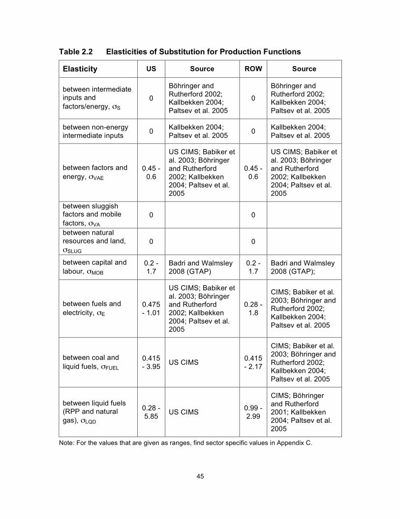
45

Table 2.2 Elasticities of Substitution for Production Functions

Elasticity US Source ROW Source

between intermediate inputs and factors/energy, !S

0

Böhringer and Rutherford 2002; Kallbekken 2004; Paltsev et al. 2005

0

Böhringer and Rutherford 2002; Kallbekken 2004; Paltsev et al. 2005

between non-energy intermediate inputs

0 Kallbekken 2004; Paltsev et al. 2005

0 Kallbekken 2004; Paltsev et al. 2005

between factors and energy, !VAE

0.45 - 0.6

US CIMS; Babiker et al. 2003; Böhringer and Rutherford 2002; Kallbekken 2004; Paltsev et al. 2005

0.45 - 0.6

US CIMS; Babiker et al. 2003; Böhringer and Rutherford 2002; Kallbekken 2004; Paltsev et al. 2005

between sluggish factors and mobile factors, !VA

0 0

between natural resources and land, !SLUG

0 0

between capital and labour, !MOB

0.2 - 1.7

Badri and Walmsley 2008 (GTAP)

0.2 - 1.7

Badri and Walmsley 2008 (GTAP);

between fuels and electricity, !E

0.475 - 1.01

US CIMS; Babiker et al. 2003; Böhringer and Rutherford 2002; Kallbekken 2004; Paltsev et al. 2005

0.28 - 1.8

CIMS; Babiker et al. 2003; Böhringer and Rutherford 2002; Kallbekken 2004; Paltsev et al. 2005

between coal and liquid fuels, !FUEL

0.415 - 3.95

US CIMS 0.415 - 2.17

CIMS; Babiker et al. 2003; Böhringer and Rutherford 2002; Kallbekken 2004; Paltsev et al. 2005

between liquid fuels (RPP and natural gas), !LQD

0.28 - 5.85

US CIMS 0.99 - 2.99

CIMS; Böhringer and Rutherford 2001; Kallbekken 2004; Paltsev et al. 2005

Note: For the values that are given as ranges, find sector specific values in Appendix C.

46

As shown in Table 2.2, I use the CIMS-based ESUB values where

possible, especially for those related to energy. For the ESUB between factors

and energy, !VAE, I used CIMS-based ESUB values for the sectors where CIMS

represents the factors more accurately. However, for some of the sectors, CIMS

does not represent the factors as accurately, so I used ESUB values that were

an average of those from the referenced models. For the ESUB between fuels

and electricity, !E, I used the US CIMS-based values directly where possible for

the US and the CIMS-based values for ROW. However, for some sectors,

including refined petroleum products and transportation, the ESUB calculations

produced nonsensical values and for these I used an average value from the

models referenced. The range of the !E values from the other models was 0.1 to

1, with multiple values near 0.4 to 0.5. For the ESUBs between coal and liquid

fuels, !FUEL, and between RPP and natural gas, !LQD, I used the US CIMS-based

values for the US. For these ESUBs in the ROW region I used CIMS-based

values, but for the sectors that had lower values than the other models I

surveyed, I used the average of the ESUBs from those models, which were

between 0.5 and 1 for !FUEL and between 1 and 2 for !LQD.

As shown in Table 2.3, I used US CIMS-based values for the ESUBs

between RPP and household fuels, !E, and between natural gas and electricity,

!HOU, for the US region. In the ROW region for !E, I used an average of the CIMS

value and those from other models as the CIMS value is based on Canada and

the others are from international models. These other models had values

between 0.3 and 0.4 for !E. I used the CIMS-based ESUB, !HOU, for the ROW

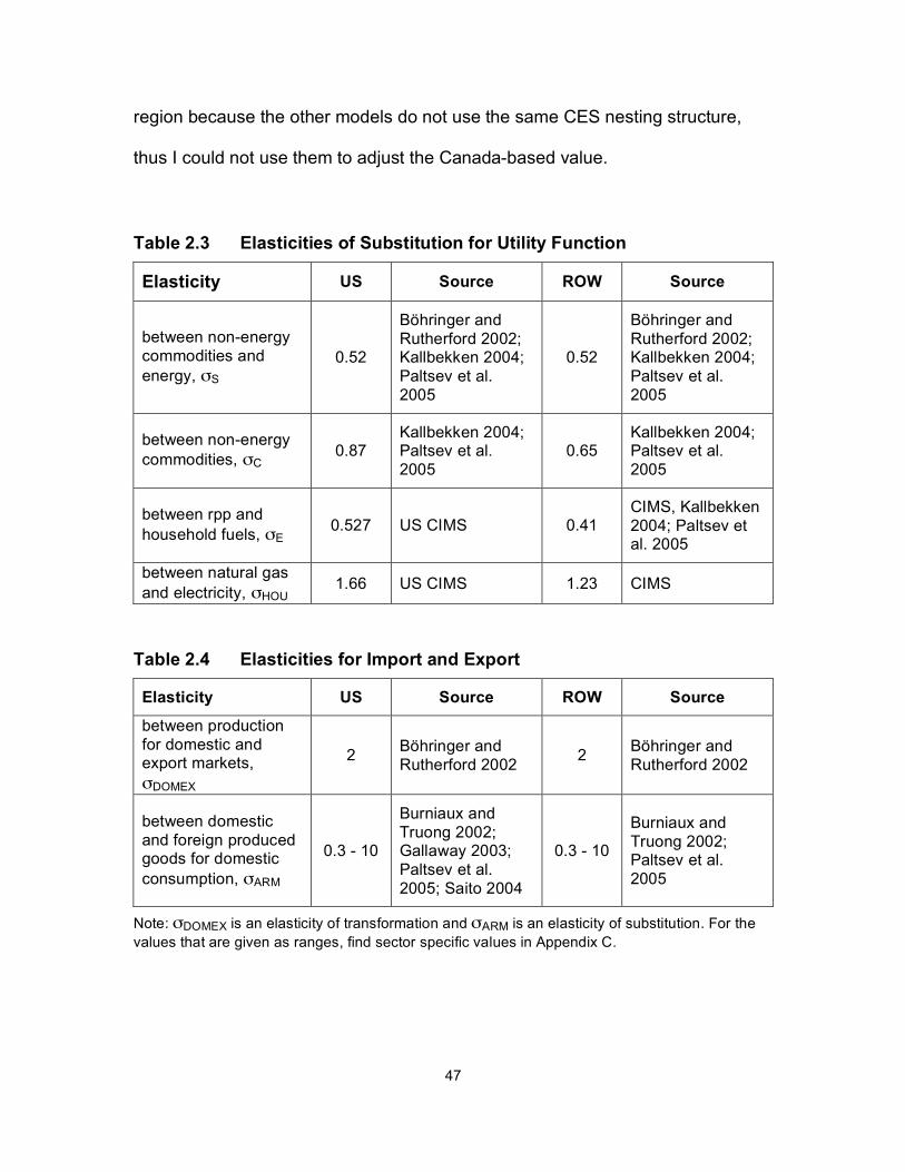
47

region because the other models do not use the same CES nesting structure,

thus I could not use them to adjust the Canada-based value.

Table 2.3 Elasticities of Substitution for Utility Function

Elasticity US Source ROW Source

between non-energy commodities and energy, !S

0.52

Böhringer and Rutherford 2002; Kallbekken 2004; Paltsev et al. 2005

0.52

Böhringer and Rutherford 2002; Kallbekken 2004; Paltsev et al. 2005

between non-energy commodities, !C

0.87 Kallbekken 2004; Paltsev et al. 2005

0.65 Kallbekken 2004; Paltsev et al. 2005

between rpp and household fuels, !E

0.527 US CIMS 0.41 CIMS, Kallbekken 2004; Paltsev et al. 2005

between natural gas and electricity, !HOU

1.66 US CIMS 1.23 CIMS

Table 2.4 Elasticities for Import and Export

Elasticity US Source ROW Source

between production for domestic and export markets, !DOMEX

2 Böhringer and Rutherford 2002

2 Böhringer and Rutherford 2002

between domestic and foreign produced goods for domestic consumption, !ARM

0.3 - 10

Burniaux and Truong 2002; Gallaway 2003; Paltsev et al. 2005; Saito 2004

0.3 - 10

Burniaux and Truong 2002; Paltsev et al. 2005

Note: !DOMEX is an elasticity of transformation and !ARM is an elasticity of substitution. For the values that are given as ranges, find sector specific values in Appendix C.

48

2.5 Analysis

The previous sections describe how I built VERITAS-US. In this section, I

describe the climate policy scenarios I analyze to meet the second research

objective and answer my research questions.

In my analysis of the policy case described below, I focus on the potential

cost of meeting the GHG emission reduction targets. This study is not a full cost-

benefit analysis of the policy cases I simulate because I do not attempt to

analyze any benefits that may be produced from the reduction of GHG

emissions. The obvious benefit of reducing GHG emission is mitigating climate

change, but there are other potential benefits like reducing local air pollutants,

including particulates, from fossil fuel combustion.

2.5.1 Policy Simulation Cases and Assumptions

Core Policy Case

The main policy case I analyze is an approximation of the American Clean

Energy and Security Act of 2009, based on my model’s ability to represent

various parts of the bill. I focus on Title III, the Reducing Global Warming

Pollution portion of the bill and do not analyze the other four titles: Clean Energy,

Energy Efficiency, Transitioning to a Clean Energy Economy, Agriculture and

Forestry Related Offsets. Details about these other sections of the bill, which

mandate standards and regulations (such as renewable electricity standards,

clean transportation standards, building, lighting, transportation and industrial

49

efficiency regulations, green job and worker transition regulations) can be found

in the summary by Larsen et al. (2009a).

The Reducing Global Warming Pollution portion of the bill provides details

for a mandatory GHG emission cap-and-trade system. The targets for this

emission cap are based on reductions from 2005 emission levels and are as

follows:

• 2012 - reduce emissions to 3% below 2005 (~12% above 1990

emission levels)

• 2020 - reduce emissions to 17% below 2005 (~4% less than 1990)

• 2030 - reduce emissions to 42% below 2005 (~33% less than 1990)

• 2050 - reduce emissions to 83% below 2005 (~80% less than 1990)

In the bill, these targets apply collectively to carbon dioxide, methane,

nitrous oxide, sulphur hexafluoride, perfluorocarbons and nitrogen trifluoride.

Since my model currently only tracks carbon dioxide, I do not analyse the other

GHGs. The bill assumes that by 2016, the cap covers approximately 84.5% of

total US emissions. For my analysis, I assume that the cap covers 100% of the

US emissions from fossil fuel use.

The American Clean Energy and Security Act has a detailed permit

allocation scheme, which I represent in my model by grouping permit allocations

into three categories that benefit: domestic consumers, domestic industrial

sectors and other countries. Table 2.5 shows the proportion of the total permit

value that I allocated to various sectors and the proportion of total US permit

50

value that is allocated to the ROW region, based on the permit distribution in the

bill. In reality, international allocation of funds would go to developing countries,

but in my model this goes to the ROW region without distinction between

developing and developed countries.

Table 2.5 Carbon Permit Allocation for Core Policy

Year Electricity

Sector

Metal

Industrial

Sector

Non-Metal

Industrial

Sector

International

Allocation

(US to ROW)

2020 35.5% 3.7% 9.7% 7%

2030 - 1.9% 4.8% 11%

2040 - - - 10%

2050 - - - 10%

The values in the rows in Table 2.5 for each year do not add up 100% and

the permit value that is not allocated to industrial sectors or for international aid is

given to the consumers. The permit value given to the electricity sector is given

as a subsidy on electricity output, with the goal of mitigating impacts of prices

increases on the consumers. The other two industrial sectors were selected

because they have the highest energy intensity in the 2004 model run. Energy

intensity (i.e. energy use per unit of output) is one of the criteria that the bill uses

to determine which sectors maybe impacted more and thus require extra aid in

the form of free permit allocations. In the model, this is represented by output-

based allocation of revenue, which essentially subsidizes the output of these

sectors.

51

The reasoning behind allocating revenue to industry revolves around the

issue of maintaining industry competitiveness and the uneven application of

emission reduction policies. An international example is that if the US enacts a

climate change policy that is more stringent than other counties, US industries

may suffer from a lack of competitiveness compared to similar industries in the

counties with less stringent emissions policies. The disparity in policy strength

may also result in the carbon or energy-intensive industries moving to the

counties with weaker emission policies, which is an example of ‘carbon-leakage’.

By subsidizing energy-intensive industrial production, the policy designers

attempt to address these competitiveness and carbon-leakage issues (Bernard et

al., 2007).

The bill also allows for the trading of emission permits with other regions

that have similarly stringent cap-and-trade policies for GHGs. I included this in

my model by allowing the US and ROW to trade emission permits. Because of

this international trading, there is only one permit price for the whole globe in the

core policy case.

There are other aspects of the bill’s cap-and-trade system that I have not

included in my analysis due to limitations in the model structure. For example, I

do not include banking and borrowing of permits or a strategic reserve of permits

as these would require a time component that is not part of the static modelling

framework of VERITAS-US. I also do not include the effects of offsets because

52

the model does not have the ability to simulate them.5 However, offsets are an

important issue and I address them briefly later in this report.

To run a policy analysis, I assume that the rest of the world will have

climate policy that aims to reduce GHG emissions. I set the ROW emission

reduction pathway so that each year they reduce the same percent from their

business-as-usual (BAU) emission levels as the US. For example, in 2020, if the

US reduces emissions to 21% below their BAU emissions, the ROW region will

also reduce emissions by 21% from their BAU. Because ROW emissions grow

faster than US emissions in the BAU case, ROW will not reach the same percent

emission reduction below 1990 levels as the US. However, in this scenario the

two regions reach a combined reduction of 65% below 1990 emissions levels by

2050. This is in the middle of the emission reduction range recommended for

stabilizing atmospheric CO2e at 450ppm, which scientists believe could keep

temperature change below 2.0-2.4oC (IPCC, 2007a).

The Clean Energy Jobs and American Power Act (Kerry-Boxer bill before

US Senate) contains elements that are quite similar to the American Clean

Energy and Security Act (Waxman-Markey bill passed by House of

Representatives). One of the main differences, and the one that I test in my

modelling of the core policy run for 2020, is that the Clean Energy Jobs and

5 An offset is an emission reduction credit that is often associated with cap-and-trade systems. An

emitter that is not covered by the cap can reduce emissions and then sell the reductions to an emitter that is covered by the cap. For example, a farmer could change her land use practices to reduce her emissions and then sell the emission reduction credit to an electricity plant with the reduction counting towards the electricity plant’s reductions. Essentially it involves the electricity plant paying someone else to reduce emissions instead of doing it themselves. The attractiveness of offsets is based on them being less expensive than the purchaser’s emission abatement costs.

53

American Power Act proposes a slightly more stringent cap of 20% below 2005

by 2020. For a summary of this bill see Larsen et al. (2009b).

The next paragraphs describe alternate variations on this core policy case,

which help define the impacts of revenue recycling to industry and international

permit trading. In all three variations of the core policy, there is allocation of

international aid from the US to ROW.

No International Permit Trading - In this variation of core policy case,

trading of permits between regions is not allowed, so each region must meet their

targets without trading permits with the other region. The emission pathway

remains the same and there is output-based allocation of revenue to industry in

both regions.

No Revenue Recycling to Industry - This variation has international

permit trading like the core policy case, but there is no revenue recycling to

industries. Essentially, this is like a cap-and-dividend system where all the

permits are auctioned and the revenue is allocated to the consumers.

No Revenue Recycling to Industry or International Permit Trading -

This variation of the core policy does not allow for international trading of permits,

so again each region must meet their targets without trading permits outside of

the region. This scenario also allocates all revenue to consumers in a cap-and-

dividend manner and thus does not have revenue recycling to industries.

54

3: SIMULATION RESULTS

In this chapter, I present key results from the model simulations and

Section 3.1 includes results from the business-as-usual (BAU) scenario. I present

marginal abatement curves for the US in Section 3.2. In Section 3.3, I show the

results from analysis of some current US legislation. Section 3.4 provides the

results from a sensitivity analysis of the ESUBs and some parameters in the CCS

sector. Throughout this chapter, I display results for the US, as it is the focus of

this project and the ROW region in VERITAS-US is quite aggregated.

3.1 Business-as-Usual Simulation Results

The BAU simulation shows the model’s representation of the economy if

the regions continue on their current paths without GHG emission reduction

policies. The data and assumptions in the data treatments described in Section

2.4 have a significant role in shaping the BAU simulation. The BAU is important

as it gives a baseline that the scenarios with GHG emission reduction policies

are compared against. The amount of CO2 emissions a region produces and the

gross domestic product (GDP) of a region are two measures that I use to

compare BAU and policy simulations.

The CO2 emissions in VERITAS-US are from the combustion of fossil

fuels, with US emissions shown in Figure 3.1. These emissions are based on the

fossil fuel use forecast from the Updated Annual Energy Outlook, so Figure 3.1

55

incorporates the impacts of the American Recovery and Reinvestment Act and

recently changing macroeconomic environment (EIA, 2009c). The CO2 emissions

in the US increase at a rate of 0.36% per year from 2010 to 2050.

Figure 3.1 US Business-as-Usual CO2 Emissions

In the BAU run of VERITAS-US, the CO2 emissions from fossil fuel use in

the ROW region grow from 22.76 Gt in 2004 to 46.05 Gt in 2050. This growth is

equal to an average increase of 1.18% per year from 2004 to 2050.

The US GDP in the model’s BAU run, shown in Figure 3.2, grows from

11.44 to 34.05 trillion 2004 US$ from 2004 to 2050. The average annual percent

increase of GDP in the US during this period is 2.4%. The GDP of the ROW

region in the BAU model run grows from 26.90 to 130.92 trillion 2004 US$ over

the period of 2004 to 2050, which represents an average annual GDP increase of

3.5%.

56

Figure 3.2 US Business-as-Usual Gross Domestic Product

3.2 Marginal Abatement Cost Curves

Marginal abatement cost (MAC) curves provide a visual representation of

the relationship between emission reductions and the cost of carbon permits.

Marginal abatement cost refers to the cost of reducing emissions by an additional

unit. A MAC curve can be made by graphing the cost of a carbon permit against

corresponding emission reductions for a given time and region (Morris et al.,

2008).

While MAC curves can provide a simple visualization of the relationship

between emissions reductions and permit prices, they can also be misleading,

especially when used with multi-regional models. The curves are sensitive to

conditions, for example policies, in the other regions in the model. They are also

affected by the types of GHGs that are included in the model as inclusion of more

57

types of GHGs expands the abatement opportunities, especially in the lower

range of marginal abatement cost. Therefore, MAC curves should be used with

caution, and only interpreted in the context of the specific policies applied when

the model is run to generate a curve (Morris et al., 2008).

To create the MAC curves for the US in Figure 3.3, I assumed that ROW

would also have a carbon abatement policy. In the curve for 2020, ROW is fixed

at a reduction of 20.9% below the model BAU, while in the 2050 curve ROW is

fixed at a reduction of 85.7% below the model BAU. These percent reductions

are consistent with those used in the policy simulations in the rest of this report.

Also, the model was set so there was neither revenue recycling to industry nor

international trading of permits. By prohibiting international permit trading, we can

see the marginal abatement cost of reducing emissions in the US specifically.

Figure 3.3 US Marginal Abatement Cost Curves

58

There are a couple of things to keep in mind with Figure 3.3. First, the

emissions reductions are relative to 2005 emissions levels. Second, the

emissions forecasted for 2050 are higher than the emissions forecasted for 2020.

Therefore, the absolute amount of emissions that is reduced at each point on the

2050 curve is larger than the amount reduced at each point on the 2020 curve.

This difference complicates a direct comparison; however, even though more

reductions are required in the 2050 curve, the price of permits is generally equal

to or less than the price in the 2020 curve. This is because in the 2050 run there

is more flexible capital available, which makes the emissions reductions easier

than they are in the 2020 run. Another trend that the MAC curves show is that the

price of permits increases significantly at emissions reductions beyond 60%

below business-as-usual. This indicates an increasingly higher cost for each

additional unit of emissions reduction as the cheaper options are used up.

3.3 Policy Simulation Results

The emission reduction pathway for the approximation of the American

Clean Energy and Security Act that I use in my analysis is shown in Figure 3.4.

This shows the targets set out in the bill for 2012, 2020, 2030 and 2050. I

assume a linear emissions reduction between 2030 and 2050, as the bill does

not set a target specifically for the year 2040. This pathway does not take into

account the offsets allowed in the bill.

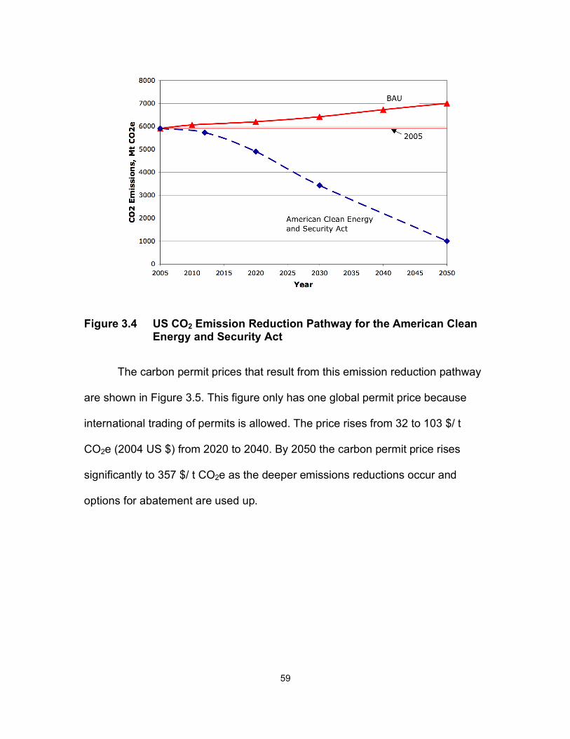
59

Figure 3.4 US CO2 Emission Reduction Pathway for the American Clean Energy and Security Act

The carbon permit prices that result from this emission reduction pathway

are shown in Figure 3.5. This figure only has one global permit price because

international trading of permits is allowed. The price rises from 32 to 103 $/ t

CO2e (2004 US $) from 2020 to 2040. By 2050 the carbon permit price rises

significantly to 357 $/ t CO2e as the deeper emissions reductions occur and

options for abatement are used up.

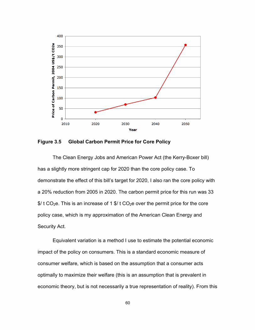
60

Figure 3.5 Global Carbon Permit Price for Core Policy

The Clean Energy Jobs and American Power Act (the Kerry-Boxer bill)

has a slightly more stringent cap for 2020 than the core policy case. To

demonstrate the effect of this bill’s target for 2020, I also ran the core policy with

a 20% reduction from 2005 in 2020. The carbon permit price for this run was 33

$/ t CO2e. This is an increase of 1 $/ t CO2e over the permit price for the core

policy case, which is my approximation of the American Clean Energy and

Security Act.

Equivalent variation is a method I use to estimate the potential economic

impact of the policy on consumers. This is a standard economic measure of

consumer welfare, which is based on the assumption that a consumer acts

optimally to maximize their welfare (this is an assumption that is prevalent in

economic theory, but is not necessarily a true representation of reality). From this

61

assumed optimal starting point, equivalent variation is an increase or decrease in

income that would be necessary to produce the same consumer welfare level

that the policy produces. In other words, the consumer would be indifferent to the

new policy situation versus a new adjusted income. Figure 3.6 shows the percent

change in US equivalent variation from the BAU situation because of the core

policy. In 2020, there is a slight equivalent variation increase of 0.1%, which is

likely related to international trading and the impacts of the different policy

strengths in the US and ROW. The decreases in equivalent variation in 2030 and

2040 are -0.3% and -0.4%, and in 2050 the decreases is -1%. This means that in

the BAU run for 2050, the consumer welfare was at 100% and in the policy run

for 2050 it is at 99% of the BAU welfare.

Figure 3.6 US Equivalent Variation % Decrease for Core Policy

Change in gross domestic product (GDP) relative to the BAU GDP is

another way to measure the economic impact of a policy and Figure 3.7 shows

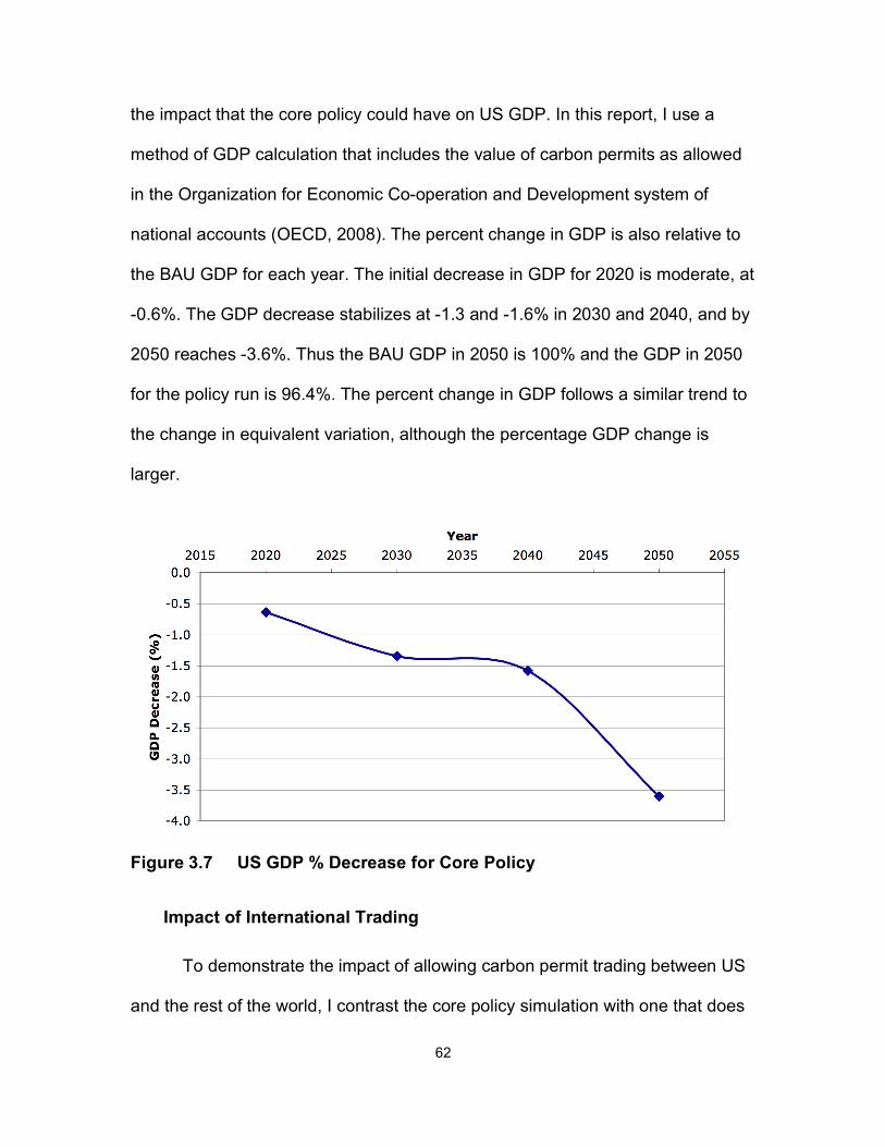
62

the impact that the core policy could have on US GDP. In this report, I use a

method of GDP calculation that includes the value of carbon permits as allowed

in the Organization for Economic Co-operation and Development system of

national accounts (OECD, 2008). The percent change in GDP is also relative to

the BAU GDP for each year. The initial decrease in GDP for 2020 is moderate, at

-0.6%. The GDP decrease stabilizes at -1.3 and -1.6% in 2030 and 2040, and by

2050 reaches -3.6%. Thus the BAU GDP in 2050 is 100% and the GDP in 2050

for the policy run is 96.4%. The percent change in GDP follows a similar trend to

the change in equivalent variation, although the percentage GDP change is

larger.

Figure 3.7 US GDP % Decrease for Core Policy

Impact of International Trading

To demonstrate the impact of allowing carbon permit trading between US

and the rest of the world, I contrast the core policy simulation with one that does

63

not allow international carbon permit trading. The permit prices of both

simulations are shown in Figure 3.8. When the US is not allowed to trade with

ROW, the US permit price is comparable to the global price in 2020 and 2030. By

2040 the US price is about 30 $/t CO2e higher than the global price. In 2050 the

US price is 484 $/t CO2e, which is 127 $/t CO2e higher than the global price of

357 $/t CO2e.

Figure 3.8 Carbon Permit Prices With and Without International Permit Trading

The welfare impacts of these policy cases are shown in Figure 3.9 and

Figure 3.10 as percent change in equivalent variation and GDP. The percent

change of equivalent variation in both cases follows a similar trend, although the

case that involves trading of permits has a slightly larger percent decrease in

equivalent variation. When permits are traded between regions, the values of

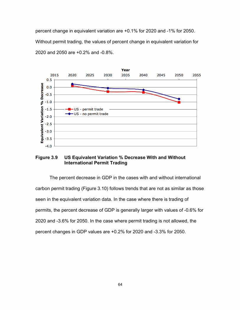
64

percent change in equivalent variation are +0.1% for 2020 and -1% for 2050.

Without permit trading, the values of percent change in equivalent variation for

2020 and 2050 are +0.2% and -0.8%.

Figure 3.9 US Equivalent Variation % Decrease With and Without International Permit Trading

The percent decrease in GDP in the cases with and without international

carbon permit trading (Figure 3.10) follows trends that are not as similar as those

seen in the equivalent variation data. In the case where there is trading of

permits, the percent decrease of GDP is generally larger with values of -0.6% for

2020 and -3.6% for 2050. In the case where permit trading is not allowed, the

percent changes in GDP values are +0.2% for 2020 and -3.3% for 2050.

65

Figure 3.10 US GDP % Decrease With and Without International Permit Trading

For both the GDP and equivalent variation, the case with no international

permit trading shows a smaller percent decrease. This means that the case with

the higher carbon permit price has less negative impact on GDP and equivalent

variation than the case with the lower carbon price and international trading. This

result for the two metrics for consumer welfare is unexpected and I present

possible explanations in the Discussion section.

Impact of Revenue Recycling to Industry

To demonstrate the impact that output-based allocation of revenue to

industry has on the carbon permit price and economic welfare, I focus on the

simulations where permit trading between regions is not allowed and contrast

those with and without output-based allocation of revenue to industry. When

there is revenue recycling to industry in VERITAS-US, the portion of revenue that

is not specifically designated to industry sectors is given directly to the consumer.

66

This case, with output-based allocation of revenue to industry, is contrasted with

the situation without revenue allocation to industry where all revenue is given to

the consumer, as in a cap-and-dividend scheme.

The carbon permit prices for the US with and without output-based

allocation of revenue to industry are displayed in Figure 3.11. In this figure, I only

display the results from 2020 and 2030 as the allocation of permits to industry

does not extend to 2040 and 2050 in the American Clean Energy and Security

Act. In 2020, when there is more allocation of revenue to industry than in 2030,

there is a larger difference in the two permit prices; with output-based allocation

of revenue to industry the carbon permit prices is 39 $/t CO2e and without it the

permit price is 35 $/t CO2e. In 2030, when the amount of revenue allocated to

industry is smaller, the permit price with and without revenue allocation to

industry is essentially the same at 83 $/t CO2e.

67

Figure 3.11 US Carbon Permit Price With and Without Output-Based Allocation of Revenue to Industry

The welfare and GDP impacts of the policy with or without output-based

revenue allocation to industry are minimal enough that they are indiscernible on a

graph.

I also looked at the impact of output-based allocation of revenue to

industry when permits are allowed to be traded between the US and ROW. In

2020 the global carbon permit price with revenue allocation to industry is 2.7 $/t

CO2e higher than the global carbon permit price without revenue allocation to

industry. The impact of output-based allocation of revenue to industry on the

global carbon price in 2030 is negligible.

68

3.4 Sensitivity Analysis

The results from CGE models are generally sensitive to the parameters

used in them, especially the ESUBs. To answer my final research question, I

carry out a sensitivity analysis on the ESUBs and on some of the key

assumptions I made about CCS in the alternate electricity sector.

Elasticity of Substitution Values

For the ESUB sensitivity analysis model runs, I compare the results from

the sensitivity analysis runs with those of the core policy simulation. To test how

robust the model is to ESUB values, I run the model in 2050 with the ESUBs

values changed by +/- 40%. I chose this range because many of the ESUB

values in the various models I surveyed were generally within it. I chose to run

the model in the 2050 time period because it was the final time period that I use

the model to analyze. The results of this analysis are shown in Table 3.1.

Table 3.1 Sensitivity Analysis of ESUB Values for 2050 Simulation

Change in ESUBs

Change in Global

Permit Price

Change in US

Equivalent Variation

Change in US GDP

+ 40% - 46.2% + 0.4% + 1.6 %

- 40% + 211.8% - 2.2% - 7.4%

The results of this analysis show that the model’s response to policies is

quite sensitive to changes in ESUB values. In general, changes in ESUBs affect,

69

in percentage terms, the carbon permit price much more than the GDP or

equivalent variation and the decrease in ESUB values had a particularly large

impact on the permit price. The confidence I have in the model results would be

improved by using CIMS-based ESUBs that have gone through more rigorous

testing procedures. The Energy and Materials Research Group at Simon Fraser

University is currently working on testing the impact that various parameters in

the CIMS model have on the ESUBs values calculated from CIMS data.

CCS Costs and Capacities

I made multiple assumptions when building the CCS alternative electricity

sector and I test some of these assumptions to determine how sensitive the

model is to them. The various components of CCS, like capture, transport and

storage of CO2, have been used separately in commercial settings, generally by

the oil and gas industry. However, the use of all the CCS components together

as one scaled-up system with the goal of preventing CO2 from entering the

atmosphere is still in the demonstration phase, of which there are currently four

operational commercial facilities (IEA, 2009). Because of the uncertainty about

the rate of widespread deployment of CCS, I run VERITAS-US in 2050 with

changes to the amount of CCS available. This analysis includes the cases where

there is 40% less CCS capacity available, 40% more CCS and also no CCS

allowed in the model. Because CCS is still in the early phases of demonstration

and the cost projections are uncertain, I also test a 40% increase and a 40%

decrease for the CCS costs in 2050.

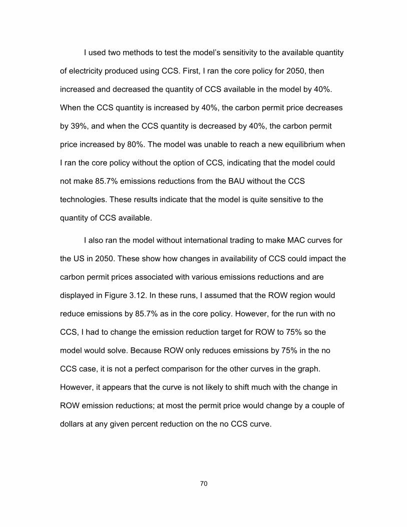
70

I used two methods to test the model’s sensitivity to the available quantity

of electricity produced using CCS. First, I ran the core policy for 2050, then

increased and decreased the quantity of CCS available in the model by 40%.

When the CCS quantity is increased by 40%, the carbon permit price decreases

by 39%, and when the CCS quantity is decreased by 40%, the carbon permit

price increased by 80%. The model was unable to reach a new equilibrium when

I ran the core policy without the option of CCS, indicating that the model could

not make 85.7% emissions reductions from the BAU without the CCS

technologies. These results indicate that the model is quite sensitive to the

quantity of CCS available.

I also ran the model without international trading to make MAC curves for

the US in 2050. These show how changes in availability of CCS could impact the

carbon permit prices associated with various emissions reductions and are

displayed in Figure 3.12. In these runs, I assumed that the ROW region would

reduce emissions by 85.7% as in the core policy. However, for the run with no

CCS, I had to change the emission reduction target for ROW to 75% so the

model would solve. Because ROW only reduces emissions by 75% in the no

CCS case, it is not a perfect comparison for the other curves in the graph.

However, it appears that the curve is not likely to shift much with the change in

ROW emission reductions; at most the permit price would change by a couple of

dollars at any given percent reduction on the no CCS curve.

71

Figure 3.12 US Marginal Abatement Curve 2050 - Change in Quantity of CCS Available

The MAC curves show that the available quantity of CCS has a large

impact on the carbon permit price. As the quantity of available CCS capacity

increases, the cost of carbon permits decreases especially with targets for

deeper emission reductions.

The cost of CCS technologies is also an area of uncertainty and to test the

sensitivity of VERITAS-US to these costs, I ran the model for 2050 using the core

policy settings with the cost of CCS increased and decreased by 40%. I found

that when the cost of CCS is increased by 40% in 2050, the carbon permit prices

increases by 6.3%. When I decreased the cost of CCS, the carbon permit price

decreased by 16.4%. This shows that the permit price is somewhat sensitive to

the cost of CCS. I also ran the model without international permit trading to

create MAC curves for the US in the 2050 time period. In these runs, ROW is

72

assumed to reduce emissions by 85.7%, which is the same as the core policy.

These MAC curves, in Figure 3.13, show the impact of changing the cost of CCS

on the carbon permit price.

Figure 3.13 US Marginal Abatement Curve 2050 - Change in Cost of CCS

This analysis shows that the permit price is marginally sensitive to the

change in CCS costs and that most of the sensitivity occurs in the range of

percent reductions below 55%. In this range, the permit price follows similar

trends to the cost of CCS, where an increase in CCS cost corresponds to an

increase in permit price. This is likely because the model is actively taking up the

first two steps of CCS in this range. For 60% emissions reductions and higher,

the CCS cost changes do not affect the permit price as much because the uptake

of CCS slows dramatically. This occurs because the capacity of the first two

steps is used up and biomass CCS becomes increasingly expensive because of

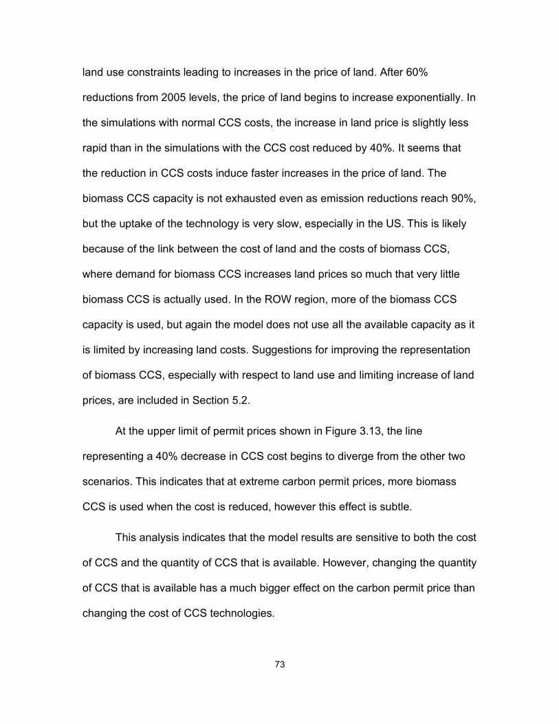
73

land use constraints leading to increases in the price of land. After 60%

reductions from 2005 levels, the price of land begins to increase exponentially. In

the simulations with normal CCS costs, the increase in land price is slightly less

rapid than in the simulations with the CCS cost reduced by 40%. It seems that

the reduction in CCS costs induce faster increases in the price of land. The

biomass CCS capacity is not exhausted even as emission reductions reach 90%,

but the uptake of the technology is very slow, especially in the US. This is likely

because of the link between the cost of land and the costs of biomass CCS,

where demand for biomass CCS increases land prices so much that very little

biomass CCS is actually used. In the ROW region, more of the biomass CCS

capacity is used, but again the model does not use all the available capacity as it

is limited by increasing land costs. Suggestions for improving the representation

of biomass CCS, especially with respect to land use and limiting increase of land

prices, are included in Section 5.2.

At the upper limit of permit prices shown in Figure 3.13, the line

representing a 40% decrease in CCS cost begins to diverge from the other two

scenarios. This indicates that at extreme carbon permit prices, more biomass

CCS is used when the cost is reduced, however this effect is subtle.

This analysis indicates that the model results are sensitive to both the cost

of CCS and the quantity of CCS that is available. However, changing the quantity

of CCS that is available has a much bigger effect on the carbon permit price than

changing the cost of CCS technologies.

74

4: DISCUSSION

The previous chapter displayed key results from the VERITAS-US model

simulations. In this chapter, I examine these results and in some cases compare

them to findings from other models. In Section 4.1, I compare the VERITAS-US

business-as-usual (BAU) and policy simulations to the reference cases and

policy simulations of other models. This section also includes a discussion of the

importance of offsets in emission reduction policies. In Section 4.2, I discuss the

implications of international permit trading and revenue recycling to industry in

the VERITAS-US policy simulations. In Section 4.3, I address the uncertainty

inherent in this project. I discuss some of the limitations and challenges of using

a static CGE model to analyze policies over long timeframes in Section 4.4.

4.1 Comparison with Other Models

4.1.1 Business-as-Usual CO2 Emissions and GDP

The BAU simulation case is very important when using models to analyze

policy because the BAU emissions are the basis for the magnitude of reductions

necessary to meet targets. The BAU economic circumstances are also the basis

for estimating the potential economic impacts of the policies. In this section, I

compare the BAU simulation of VERITAS-US to the reference cases of other

similar models.

75

I compare the US GDP in the BAU run of VERITAS-US to the reference

case GDP in the MIT-EPPA6 and ADAGE7 models, as shown in Figure 4.1. The

three forecasts of GDP are quite similar as the ADAGE and MIT-EPPA GDP are

within 5% of VERITAS-US GDP from 2010 to 2040. It is only in 2050 when the

MIT-EPPA forecast is beyond this range and is 7% larger than the VERITAS-US

GDP.

Figure 4.1 Comparison of Business-as-Usual GDP for the US by VERITAS, MIT-EPPA and ADAGE

Sources: Paltsev et al. (2009) and Ross (2008)

6 MIT-EPPA is a recursive-dynamic multi-regional general equilibrium model of the world

economy. It is developed and used by the Joint Program on the Science and Policy of Global Change at the Massachusetts Institute of Technology. MIT-EPPA is designed to develop projections of economic growth and anthropogenic emissions of greenhouse related gases and aerosols and can be used in conjunction with the MIT Integrated Global Systems Model (Paltsev et al., 2005).

7 ADAGE is a dynamic computable general equilibrium model capable of examining many types of economic, energy, environmental, climate-change mitigation and trade policies at the international, national, U.S. regional and U.S. state levels. It is developed by RTI International (Ross, 2008).

76

The BAU CO2 emissions of VERITAS-US are compared to reference case

CO2 emission in the MIT-EPPA, ADAGE and EIA-NEMS8 models in Figure 4.2.

The CO2 emissions for EIA-NEMS and VERITAS-US are based on fossil fuel

combustion only, whereas the MIT-EPPA and ADAGE data in the figure show

CO2 from fossil fuel combustion and CO2 from non-combustion sources, like

agriculture and industrial processes. The CO2 emissions from VERITAS-US

match the MIT-EPPA and EIA-NEMS forecasts fairly well in the first few decades,

however the MIT-EPPA emissions are 24% higher than the VERITAS-US

emissions by 2050. The ADAGE data show the emissions being consistently

higher than VERITAS-US, which could be attributed to ADAGE accounting for

CO2 beyond fossil fuels use. The MIT-EPPA model also covers CO2 emissions

from sources other than fossil fuel use, but I think it is unlikely that the MIT-EPPA

difference in emissions in 2050 is solely because of non-fossil fuel CO2

emissions as it increases more rapidly in the later decades. The emissions in the

VERITAS-US BAU may be lower than MIT-EPPA in 2040 and 2050 because

they are based on an extrapolation of the EIA fossil fuel use data that cover 2006

to 2030. As shown in the graph, the MIT-EPPA emissions grow much faster in

the period after 2030 than the EIA-NEMS emissions in the period up to 2030.

8 The EIA-NEMS model is a technology rich, computer-based, energy-economy modelling system

of U.S. It is designed and implemented by the Energy Information Administration (EIA) of the U.S. Department of Energy. EIA-NEMS is used to project the energy, economic, environmental and security impacts of alternative energy policies on the United States (EIA, 2009e).

77

Figure 4.2 Comparison of Business-as-Usual CO2 Emissions for the US by VERITAS-US, EIA-NEMS, MIT-EPPA and ADAGE

Sources: EIA (2009b, 2009c), Paltsev et al. (2009) and Ross (2008)

4.1.2 Emission Reduction Policies

In this section, I compare the results of my policy simulations with results

from other models that have been used in similar studies. First, I compare results

from studies that do not use offsets and have emission reduction pathways

similar to my approximation of current US legislation. Next, I summarize some of

the analyses of current US legislation by models that can simulate offsets and

discuss their importance in climate change policy.

78

Comparison of Simulations Without Offsets

Ross et al. (2009), Paltsev et al. (2009) and Tuladhar et al. (2009) used

the ADAGE, MIT-EPPA and MRN-NEEM9 models to analyze an emission

reduction pathway that results in approximately 167 billion Mt of cumulative GHG

emissions between 2012 and 2050. This pathway is essentially a linear reduction

of emissions from 2012 until 2050, reaching an annual reduction of 80% below

1990 emissions levels in 2050, which is quite similar to the reduction pathway I

used in my approximation of the American Clean Energy and Security Act. The

trading of permits between international regions is not included in the studies by

Ross et al. (2009), Paltsev et al. (2009) and Tuladhar et al. (2009), so I compare

them to my simulation of VERITAS-US that does not have international trading of

carbon permits (Figure 4.3).

9 MRM-NEEM is an integration of MRM, a top-down dynamic computable general equilibrium

model, and NEEM, a technology-rich bottom-up model of the US electricity sector. This combination is developed by CRA International for analysis of US greenhouse gas policies (Tuladhar et al., 2009).

79

Figure 4.3 Comparison of Emission Permit Prices for the US by VERITAS-US, MIT-EPPA, ADAGE and MRN-NEEM

Sources: Paltsev et al. (2009), Ross et al. (2009) and Tuladhar et al. (2009)

Figure 4.3 shows a wide range in the permit prices forecasted by these

models. VERITAS-US starts out with permit prices at the low end of the

estimates in the early decades and has a permit price at the high end in 2050.

There are multiple factors that may be contributing to these results.

One reason that the other models have a smaller range and a more

gradual increase in permit prices over the time period of the policy could be that

they involve the option of banking and borrowing permits. This is a cost

containment measure that helps manage the permit price by allowing the use of

saved permits from past years and the limited use of permits from future years. In

a comparison of a policy scenario with and without banking and borrowing of

permits, Tuladhar et al. (2009) found that without banking the permit price was

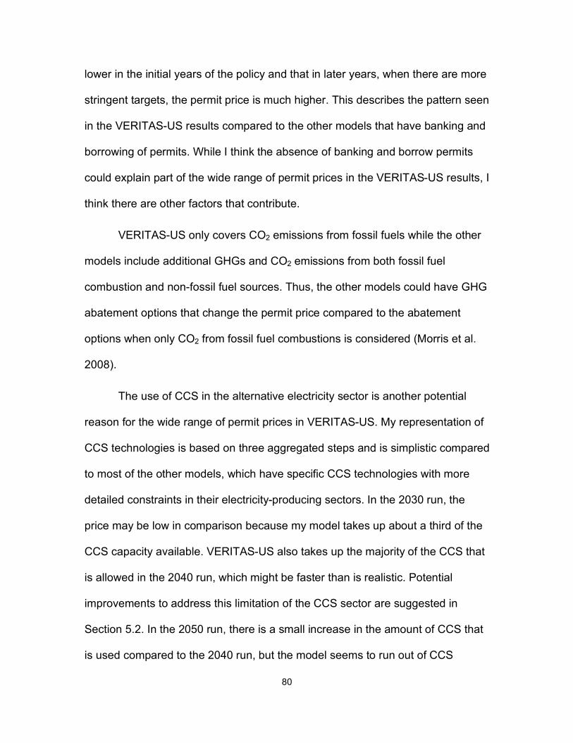
80

lower in the initial years of the policy and that in later years, when there are more

stringent targets, the permit price is much higher. This describes the pattern seen

in the VERITAS-US results compared to the other models that have banking and

borrowing of permits. While I think the absence of banking and borrow permits

could explain part of the wide range of permit prices in the VERITAS-US results, I

think there are other factors that contribute.

VERITAS-US only covers CO2 emissions from fossil fuels while the other

models include additional GHGs and CO2 emissions from both fossil fuel

combustion and non-fossil fuel sources. Thus, the other models could have GHG

abatement options that change the permit price compared to the abatement

options when only CO2 from fossil fuel combustions is considered (Morris et al.

2008).

The use of CCS in the alternative electricity sector is another potential

reason for the wide range of permit prices in VERITAS-US. My representation of

CCS technologies is based on three aggregated steps and is simplistic compared

to most of the other models, which have specific CCS technologies with more

detailed constraints in their electricity-producing sectors. In the 2030 run, the

price may be low in comparison because my model takes up about a third of the

CCS capacity available. VERITAS-US also takes up the majority of the CCS that

is allowed in the 2040 run, which might be faster than is realistic. Potential

improvements to address this limitation of the CCS sector are suggested in

Section 5.2. In the 2050 run, there is a small increase in the amount of CCS that

is used compared to the 2040 run, but the model seems to run out of CCS

81

capacity and other cheaper options for reducing emissions. This may explain why

the permit price in 2050 is so much higher than the price in 2040.

The ESUB values used in the different models are another factor that

could contribute to the difference in forecasted permit prices. The impact of

ESUB values is most likely more apparent in the 2050 results, as the uptake of

CCS in 2020 to 2040 likely has a large influence on the permit price in these

years. The ESUB values related to substituting fuels, especially those between

fuels and electricity, !E, and between coal and liquid fuels, !FUEL, seem like they

could explain part of the price range in 2050 shown in Figure 4.3. The MIT-EPPA

model has a value of 1 for both of these ESUBS, whereas the US values of !E

and !FUEL in VERITAS-US are less than 1 for most sectors. This could partly

explain the lower permit price forecast by the MIT-EPPA model in 2050 as higher

ESUB values allow for easier substitution and potentially lower permit prices. The

value of !E in the ADAGE model is 0.5, which is closer to the US values in

VERITAS-US, and might explain the similar permit prices of VERITAS-US and

ADAGE in 2050. ADAGE does not have similar nesting structure for the !FUEL

ESUB so I could not make a comparison of this parameter. The three models,

VERITAS-US, ADAGE and MIT-EPPS, have similar ESUB values, in the range

of 0.4 to 0.5, for the substitution between factors and energy, !VAE.

These models estimate similar ranges for the economic and welfare

impacts of this emissions reduction pathway. In VERITAS-US, the changes in

GDP and equivalent variation, which is a measure of welfare, are decreases of

3.1% and 0.8% in 2050. The MIT-EPPA model shows decrease in welfare of

82

2.5% in 2050 (Paltsev et al., 2009). The MRN-NEEM model shows a decrease in

GDP of 3.09% and decrease in welfare of 1.96% in 2050 (Tuladhar et al., 2009).

The ADAGE model shows the impact on GDP and welfare as a change in annual

average growth in GDP and consumption. These annual average growth rates

change from 2.31% in the BAU to 2.11% for GDP and 2.33% to 2.18% for

consumption (Ross et al., 2009). The models all show small decreases in the

GDP and welfare in 2050 because of reducing GHG emissions to 80% below

1990 levels in 2050.

Simulations With Offsets

Offsets are an important issue in GHG emission reduction policy and the

American Clean Energy and Security Act allows for the annual use of 2000 Mt

CO2e of them. Half of this amount must be acquired domestically and half can be

from international sources. To put these allowable offsets in perspective, in 2005

the US emitted approximately 7100 Mt CO2e. By allowing the use of such a

significant amount of offsets, the actual reductions required from the sectors of

the US economy covered by the cap-and-trade system are much less than if no

offset were allowed. Figure 4.4 shows the emission reduction pathway prescribed

by the targets in the bill and the amount of allowed offsets. This figure includes

GHGs beyond the CO2 from fossil fuel combustion that my model tracks.

83

Figure 4.4 Emission Reduction Pathway for the American Clean Energy and Security Act Targets With and Without Offsets

The amount of offsets included in a policy can have a large impact on the

price of emission permits. Figure 4.5 shows the emission permit prices

determined by models that analyzed the American Clean Energy and Security

Act. The MIT-EPPA model, the ADAGE model (for Environmental Protection

Agency’s analysis) and the Energy Information Administration’s NEMS model

were all used to simulate a version of the bill with full offset use and with partial

offset use, often by limiting the international offsets. In the MIT-EPPA model, it is

assumed that the price of offsets starts at 5$/t CO2e in 2015 and then increases

at 4% per year, which equals close to 20$/t CO2e in 2050 (Paltsev et al., 2009).

The ADAGE model includes the assumption that domestic offset prices are equal

to the permit price for the full-offset case, which starts at 13 $/t CO2e in 2015 and

rises to 70 $/t CO2e in 2050. The international offset prices in ADAGE are

84

assumed to be a bit lower, starting at 10 $/t CO2e in 2015 and rising to 55 $/t

CO2e in 2050 (Environmental Protection Agency, 2009). For the EIA-NEMS base

case analysis, they assume offset prices of 32 $/t CO2e in 2020 and 65 $/t CO2e

in 2030 (EIA, 2009f). The restriction of offsets to half their allowed value

increases the permit price in the MIT-EPPA and ADAGE models by about 60 $/t

CO2e (2004 US$) by 2050. The EIA model forecasts to 2030 and in this year the

permit price increases by approximately 60 $/t CO2e when offsets are restricted

to 1000 Mt CO2e.

Figure 4.5 Emissions Permit Price for the American Clean Energy and Security Act Analysis by MIT-EPPA, ADAGE and EIA-NEMS for Full Offset and Limited Offset Cases

Sources: Paltsev et al. (2009), EIA (2009f) and Environmental Protection Agency (2009)

On one hand, offsets could be viewed as beneficial because they reduce

the number of emissions reductions the capped sectors have to make by shifting

the reductions to non-capped sectors, thus reducing permit prices. On the other

85

hand, they can thwart actual emissions reductions for a couple of reasons. First,

one problem with offsets is similar to that of subsidies, which is the difficulty of

ensuring that the offsetting action would not have occurred even if the policy

were not in place. Second, there is the potential problem of trying to reduce

emissions by using offsets when they might not represent permanent reductions;

for example if trees are planted and then later cut down. If the offsets are not

additive, i.e. do no contribute real reductions in the absolute amount of a

society’s emissions, the total amount of emissions the policy reduces could be

much less significant than indicated by the targets. An example of this is the

potential of Kyoto’s Clean Development Mechanism to make it look like the

Protocol’s targets are being met, yet undermining effectiveness if the projects are

not delivering truly additional emissions mitigation (Wara, 2006). While the

American Clean Energy and Security Act requires that the offsets be accredited,

it may not be possible to guarantee that they are actually causing additional and

permanent emissions reductions.

4.2 Alternative Policy Cases

International Trading

The core policy case allows for international trading of carbon permits,

which I compare with a variation where international trading is not allowed. In the

core policy case, the global carbon permit price in 2050 is 127 $/t CO2e less than

the US carbon permit price when the US is not allowed to trade permits with the

ROW region (Figure 3.8). By allowing international trading it makes the reduction

of emissions more cost efficient for the global community as a whole. Because

86

countries that can abate emissions at lower costs will abate more than counties

with higher abatement costs, it allows for a given emission reduction target to be

reached at a lower total economic cost. This is an application of the equi-

marginal principle, which in this case asserts that the cost to society for reducing

emissions is minimized when each source of emissions (or emitting country)

reduces emissions up to the point where their marginal abatement costs of

further reductions are the same.

The comparison of VERITAS-US international trading simulations (Figure

3.9 and Figure 3.10) shows some initially counterintuitive results. First, in the

2020 simulations the equivalent variation for both permit trading cases is higher

than in the business-as-usual (BAU) case and the GDP for the case without

international permit trading is also higher than the BAU GDP. Second, the US

consumer welfare and GDP are higher when international permit trading is not

allowed compared to when it is allowed in the core policy case. This result is

unexpected, as one might think that consumers would be better off with lower

carbon permit prices. I discuss each of these anomalies in the following

paragraphs.

The increase of equivalent variation and GDP beyond the values in the

BAU simulations in the 2020 time period, are unexpected as they represent a

double dividend. Double dividend refers to the situation where the revenue from

an environmental policy is used to reduce the impacts of an already existing

distortionary tax, such as income, payroll or sales taxes, leaving the consumer

better off than before the environmental policy. The two dividends, with respect to

87

the term, are the benefits of (1) reducing environmental harm and (2) reducing

the distortionary cost of the existing tax system (Goulder, 1995). However, in

VERITAS-US there are no initial distortionary taxes in the business-as-usual

simulation, so it seems odd that there would be a double dividend situation.

There is a difference in the stringency of the emission reduction as the US and

ROW have different reduction requirements. The increase in welfare and GDP in

2020 could be explained by energy-intensive industry moving production to the

US or because of the improvement of the US terms of trade, which are the

relative price of a country’s exports to imports. Because the US is a net energy

importer, it could benefit from lower oil prices because of reduced global demand

induced by the cap-and-trade system.

Based on the results in Figure 3.9, the US consumer is slightly better off,

i.e. equivalent variation is higher, when international trading of permits is not

allowed and the carbon permit price is higher, when compared to the simulation

where international permit trading is allowed. This could potentially be explained

by improvement in the US terms of trade and changes in trading of commodities

other than emissions permits. The effects trading permits could also contribute to

this result as the US becomes a net permit buyer when international trading of

permits is allowed, which causes large flows of funds out of the US.

The structure of my model might exaggerate the effect of the lost domestic

income on consumer welfare. Because government services are not modelled

specifically, the consumer is given the revenue from all permits unless the

revenue is designated to an industrial sector. In reality, the revenue that is not

88

designated to industry could be used for many things, like green technology

development funds or reducing national debt. While these activities benefit the

consumers, they might not have as drastic welfare impacts as when the entire

amount is given directly to the consumer.

The higher GDP in the case without permit trading (Figure 3.10) may be

connected to the higher permit price associated with this case. As mentioned

before, the GDP measurement in VERITAS-US includes the value of carbon

permits, so a higher permit price could contribute to a higher value for GDP. The

lower GDP in the international trading case could also be attributed to a variation

in the model. There is a slight difference in how permits are allocated between

the global version of the model, which is used for the case with international

permit trading, and the regional version of the model, which is used for the case

that does not allow permit trading. In the global version, the number of permits

that are allocated to the international community, as part of the permit distribution

in the American Clean Energy and Security Act, are subtracted from the total

number of permits endowed to the US consumer. In the regional version, the full

amount of permits allocated to the US is endowed to the US consumer and then

a lump sum transfer of funds is made from the US consumer to the ROW

consumer to represent the bill’s allocation of permit revenue to the international

community. This means that in the regional version (no international permit

trading) the US consumer is initially endowed with more permits than in the

global version (international permit trading). Since the value of carbon permits is

included in the GDP, this difference in the method of permit endowment could

89

also contribute to the slightly higher GDP for the case without international permit

trading.

The impacts of linking a US cap-and-trade system to other international

cap-and-trade systems would likely go beyond the potential reduction in emission

permit price that my model predicts. Jaffe and Stavins (2008) describe some of

the other consequences of linking cap-and-trade systems, including that this can

limit the amount of control a government has over its country’s system. Linking

can also cause distributional effects within systems and across linked systems

that may be undesirable, such as large flows of capital between regions. It also

opens up various system attributes, like offsets and price safety valves to other

connected systems. If a system with a firm emissions cap links with one that has

an intensity-based cap, the linked systems may not achieve the same level of

emissions reductions compared to the un-linked systems. The trade offs of all

these impacts must be considered carefully when design the linkages between

cap-and-trade systems (Jaffe and Stavins, 2008).

Revenue Recycling to Industry

I also looked at output-based allocation of revenue to industry and the

impact that it could have on the cost of a policy. I found that in the 2020 and 2030

runs of the core policy simulation, the carbon permit price is higher with revenue

allocation to industry (Figure 3.11). This finding is consistent with an analysis of

output-based rebating by Fischer (2001), where she found that for a given

amount of emissions reductions, output-based rebating increases the marginal

cost of emission reduction relative to a policy without rebating. This occurs

90

because the output-based rebating leads to higher than optimal production of

output, as firms have an incentive to increase output in order to maximize the

subsidy they receive. The comparison of the 2020 simulations shows a decrease

of 4 $/t CO2e in the carbon permit price when revenue is not allocated to

industry, but rather given entirely to consumers. The output-based allocation of

revenue to industry that is considered in this case is approximately 49% of total

permit revenue and is used to subsidize electricity and industrial output.

Fischer (2001) compares the output-based allocation to industry with a

socially optimal policy, where welfare is optimized and emissions are reduced to

the point were society, as a whole, would not benefit from further reductions. In

comparison to this optimal policy, or the ‘first-best’ policy, output-based rebating

to industry decreases the economic efficiency. For my analysis of output-based

allocation of revenue to industry, I compare it with the case where all revenue is

given to the consumer. I assume that this ‘cap-and-dividend’ case is not a

socially optimal policy as it has uneven reduction requirements for the different

regions. If a policy is not socially optimal, the addition of output-based allocation

of revenue can actually improve the economic efficiency of the policy (Fischer

and Fox, 2009). In the simulations I explore for this analysis, the output-based

allocation of revenue to industry could improve the policy by increasing the

competitiveness of the US industry, which could improve US welfare, and by

preventing leakage of emissions to ROW. However, my analysis does not include

the optimization of revenue allocation amounts, so I am not certain whether the

91

output-based allocation in this simulation increases or decreases overall

economic efficiency of the policy.

Even though output-based allocation of revenue to industry increases the

carbon permit price of a policy, public and industry support for the policy will likely

be more important than the small increase in permit price. Acceptance of the

policy is especially important in the near term so the policy will actually be

implemented. In the American Clean Energy and Security Act this is addressed,

as revenue recycling to industry is included in the first years of the policy and

then phased out beginning in 2025. By 2040 and 2050 there is no revenue

recycling to industry (all revenue is given to the consumer).

To further explore the impacts of revenue recycling, beyond subsidies to

industry, I could potentially have dealt with some of the permit allocations in the

bill more realistically, by including subsidies for CCS or by lower income tax and

tax credits. These options were too detailed for the framework of my model and

went beyond the scope of this project.

4.3 Uncertainty

Modelling is inherently an uncertain practice, as each model is a

representation that never truly captures the actual system under examination. If

we try to increase the realism of our models by adding more parameters, we may

actually increase the uncertainty (Oreskes, 2003). The uncertainty related to

forecasting also generally increases as our forecasts go further into the future.

92

This section describes the main sources of uncertainty in this project and how I

accounted for them.

Structural uncertainty occurs because all models are simplified

representations of more complex real-world systems and because we use

approximations to represent these systems (Morgan and Henrion, 1990). For

example, in this project I assume that nested constant elasticity of substitution

functions represent the real world where firms produce goods and people and

firms consume goods and services. I also use an amalgamated ROW region and

assume that it represents all the countries in the world, excluding the US. Often

these assumptions accompany trade-offs between realism and the simplicity of a

model.

There is also uncertainty in the parameters that are used in models, which

involves how well a numerical variable represents elements of the system being

modelled (Oreskes, 2003). Using historical data and judgement to estimate

ESUBs and AEEI and then using them to forecast also adds uncertainty.

The data that I use also have uncertainty associated with them. While the

historical data I used are likely the least uncertain, they still have uncertainty

because of potential measurement and communication errors. The forecasted

data I used for my fossil fuel consumption were generated by another model with

all of its associated uncertainty. The extrapolation of my SAMs for use in the

various time periods that I model also increases the uncertainty from the data

used in the project.

93

There are several ways that I accounted for the uncertainty in this project.

I used established methods for constructing the model and reliable sources for

my data. I tried to decrease the uncertainty of using historically based

parameters to forecast future trends by using ESUBs from CIMS. While this

theoretically reduces uncertainty by providing ESUBs that are based on

technologies that could be used in the future, it introduces the uncertainty of

using parameters based on forecasts from estimated relationships in the CIMS

model. I also compare my results to those from models that have various

different parameter values and modelling approaches. The final way that I

address uncertainty is by subjecting VERITAS-US to a sensitivity analysis.

When using results from models like VERITAS-US, it is important to keep

in mind that specific numbers are less important than general trends. Also the

results are quite variable depending on assumptions and methods of modelling

policies. The results are heavily based on assumptions about technologies and

behaviours in the future, meaning that the model results for 2040 and 2050 are

especially vulnerable to the likelihood that the model is missing key technologies

that have not yet been invented.

4.4 Challenges of Static CGE Modelling

I briefly discussed the challenges of modelling carbon capture and storage

(CCS) in a static CGE model in the Methods section, but there are other

difficulties associated with using a static modelling framework. These difficulties

are inherent when using a static model to analyze policies over long time frames

94

as static models represent one time period per simulation and each time period is

not connected to previous or future time periods.

The main limitations and challenges of using a static model over long time

frames relate to this lack of connection between time periods. For example, the

2050 run has no dependence on capital stock built, prices, or any other aspect of

the 2040 run of the model. This lack of time continuity makes it difficult to model

processes that depend on previous actions. For example, tracking the quantity

and quality of CCS sites that are used over time is not possible in a static model.

Because of the lack of time continuity, my model also does not track investment

and savings explicitly. The time element would also be necessary for including

banking and borrowing of emission permits in the model. The data in each SAM

are also based on extrapolation from the 2004 data and are not affected by the

previous SAMs or previous impacts of the policy. These limitations must be kept

in mind when interpreting results from VERITAS-US. While there are many

limitations of using a static model, its simplicity made this research project

feasible in a reasonable time scale.

95

5: CONCLUSIONS

In this research project, I built a global energy-economy model for

analyzing climate change policy with a focus on the United States. The model is

called VERITAS-US and I built it using a static CGE framework that was

enhanced by parameters informed by CIMS technology simulation models. I

used VERITAS-US to analyze climate change policy that is currently relevant to

American and international situations. In Section 5.1 of this chapter, I review the

findings from my analysis with respect to my research questions. I present some

options for improving the VERITAS-US model and suggest directions for future

research in Section 5.2.

5.1 Summary of Research Findings

What are the potential economic and environmental impacts of currently

proposed US climate policy?

To answer this question, I did an analysis of the core policy case, which is

an approximation of the American Clean Energy and Security Act of 2009. I

found that the cost of carbon permits for my approximation of the bill without

offsets would be 32 $/ t CO2e (2004 US$) in 2020, 70 $/ t CO2e in 2030, 103 $/ t

CO2e in 2040 and 357 $/ t CO2e in 2050. I also found that the welfare of the US

consumer would decrease by 1.02% in 2050 because of the costs of the policy.

The decrease in GDP for the US under the core policy would be 3.60% in 2050.

96

This research only attempts to analyze the costs of the policy and does not

attempt to quantify the benefits.

In this project, I equate the environmental impacts of a policy with the

GHG emissions reductions the policy could cause. The core policy case involved

a reduction of GHG emissions to 83% below 2005 levels by 2050, which is

approximately an 80% reduction below 1990 levels by 2050. These reductions

are significant and would put the US well along the path required to do its part in

stabilizing the atmospheric concentrations of GHG at a level that could keep the

average global temperature increase below 2oC. However, the bill allows for a

large number of offsets, which could undermine the emissions reductions it

proposes in the targets. If the offsets used in the bill are not truly additive or

permanent, the policy’s emission reduction targets could be exceeded by up to

2000 Mt CO2e annually.

What are the potential effects of trading carbon permits internationally

versus the option of the US acting alone without international permit

trading?

I compared the core policy case, which allows international trading of

permits, with a simulation where international permit trading was not allowed. In

this second case, I found that the carbon permit price in the US increased by

about 30 $/t CO2e in 2040 and by 127 $/t CO2e by 2050. Although the carbon

permit price increased when permit trading was not allowed, I found that US GDP

and welfare were actually higher without international permit trading. GDP in

2050 was 0.3% higher without international trading than it was in the core policy

97

case. Welfare in 2050 was 0.2% higher in the case without international permit

trading. There are many other potential effects of linking a US cap-and-trade

system to international systems through trading of permits and these should be

weighed carefully when designing the structure of the linkages.

What are the potential impacts of revenue recycling or permit allocation

within the US?

I compared the core policy simulation, which uses output-based allocation

of permit revenue to approximate the American Clean Energy and Security Act’s

allocation of permits, with a simulation that allocates all the permit revenue

directly to the consumer. I found that the core policy case, with revenue recycling

to industry, required higher carbon permit prices to reach the same emission

reduction target than the case where all the revenue was recycled to the

consumer. In 2020 when about 49% of total permit revenue was recycled to

industry, the carbon permit price was 4 $/t CO2e higher than the case without

revenue recycling to industry. By 2030, a much smaller amount of total permit

revenue was given to industry and the permit price difference was negligible.

From my analysis, it seems like the potential impact of output-based allocation of

revenue to industry on the permit price is small enough that it would be worth

pursuing to increase industry support for the policy.

98

How robust is the model to different values for elasticities of substitution

and the assumptions made regarding carbon capture and storage costs

and capacity?

In my sensitivity analysis of the ESUBs in VERITAS-US, I found the model

is quite sensitive to changes in the ESUB values. The carbon permit price was

more sensitive to decreases in the ESUB values than to increases in ESUBs. In

the 2050 model run, a 40% decrease in the ESUB values caused a 212%

increase in the carbon permit prices, whereas a 40% increase in the ESUB

values caused a 46% decrease in the permit price. The ESUB value changes

also impacted the GDP and welfare but to a much lesser extent.

I also did a sensitivity analysis on the alternative electricity production

sector with CCS and I found that the model is quite sensitive to my assumptions

about the quantity of CCS available and the cost of CCS. The analysis showed

that the carbon permit price was most sensitive to changes in the quantity of

CCS available and that the cost of CCS had a smaller impact.

The main conclusions that I have drawn from this research are:

A policy that aims to achieve significant reductions in GHG emissions will

have real economic costs. In the near term the negative impact that a policy, like

the American Clean Energy and Security Act, will have on US consumer welfare

is likely to be relatively minimal. The forecasts further in the future show slightly

larger impacts on welfare but are also more uncertain.

Linking a US cap-and-trade system with other similar systems, through

international trading of permits, could decrease the cost of permits in the US.

99

However, the implications of linking a cap-and-trade system to other systems are

numerous. The types of linkages and their effects should be researched

thoroughly before implementation.

Output-based allocation of revenue to industry will increase the permit

price required to meet specific targets. However, I think that if revenue recycling

to industry increases support for a policy, it will likely be worth a small increase in

permit price, especially if it means that a policy will actually be implemented. This

would particularly hold true if the revenue recycling to industry is phased out in

later years of the policy.

My analysis looks at the total impacts on GDP and welfare because of

carbon permit prices arising from cap-and-trade systems. This does not account

for the distribution of the impacts and there are significant equity issues involved

with this. Any policy should have ways to protect those most vulnerable, for

example low-income households and those employed in sectors that are

negatively impacted by the cap-and-trade policy. Climate change policies should

also have regularly scheduled reviews and opportunities for alteration to ensure

they are meeting social, economic and environmental goals.

5.2 Future Model Development and Research

The sensitivity analysis indicated that the model is sensitive to ESUB

values and the assumptions I made regarding the CCS sector. Because of this

analysis, I suggest these key areas for improving the model:

100

• reducing the uncertainty relating to the ESUB values, especially by

testing and improving the method for generating ESUBs from CIMS

models;

• improving the alternative electricity sector and the model’s

representation of CCS. For example, include specific CCS

technologies, nuclear, renewables and improve the representation of

biomass energy and land use feedbacks and potentially add in

constraints on the increase of land prices. Also, including constraints to

limit the amount of each technology in given time periods will likely be

quite important as the model results were more sensitive to quantity of

CCS available than cost of CCS.

There are other changes that I recommend to improve VERITAS:

• include a method for modelling offsets,

• test/alter permit allocation methods in Regional and Global modes to

ensure the permit allocation methods result in consistent GDP,

• make it a dynamic model,

• include GHGs other than CO2 (like methane, nitrous oxide, sulphur

hexafluoride, perfluorocarbons),

• add CO2 emissions from cement, agriculture, waste etc.,

• make a separate agriculture sector by removing it from the Rest Of

Economy (ROE) sector,

• include investment and government separate from the consumer, and

• include a labour/leisure option for consumers.

There are many interesting areas of research that this model could

potentially be used in, especially once some of the recommended improvements

are made. If the multi-regional aspects of VERITAS were combined with the

more complicated theory of single region dynamic model, to create a multi-

101

regional dynamic model, it could eventually be linked with CIMS-Global or any

other CIMS regional model. This could help resolve some of the ESUB and CCS

technology issues in VERITAS.

It would also be interesting to focus on North America with either this

model or a dynamic version of it. This type of research could explore a North

America wide cap-and-trade system and could elaborate on how the nuances of

policy design affect the various countries involved.

102

APPENDICES

103

Appendix A: VERITAS-US Code in GAMS/MPSGE

!*VERITAS-US - a static global CGE model with trade between two regions (US and ROW) for analysis of climate change policy ! !*Base year of the model is 2004 ! !SET a(*) commodities and factors, ! i(a) commodities , ! j(*) sectors, ! fd(*) final demand, ! f(a) factors; !! !SET r /US, ROW/;! !SET a(*) /OIL, ELEC, GAS, COAL, RPP, MET, NMET, OMAN, TRANS, ROE, K, L, LN, NR /;! !SET i(a) /OIL, ELEC, GAS, COAL, RPP, MET, NMET, OMAN, TRANS, ROE/; !SET j(*) /OILJ, ELECJ, GASJ, COALJ, RPPJ, METJ, NMETJ, OMANJ, TRANJ, ROEJ/; !SET f(a) /K, L, LN, NR/; !SET FD(*) /FDEM, INV/; !ALIAS(i,ii) ; ALIAS(r,rr) ; ALIAS(j,jj); ! ! !Scalar year time period to run model in (base 2004 - other options 2010 2020 2030 2040 2050); ! !*both of these need to be changed for the model to run!! !$set year 2050 !Year = 2050; !***************change policy and Atech files too!!!!!************** ! !*Load social accouting matrix !$INCLUDE "GDX to Gams BALSAM_%year%.gms" ! ! !*Sets whether you use global or regional option, !* if OPT = 1, the model uses global abatement !* if OPT = 2, regions act alone. ! !PARAMETER !OPT Regional or global abatement option; !*When you change OPT - make sure the model loads the correct policy file (the flagging didn't work...) !*opt = 1 global !*opt = 2 regional !OPT = 1; ! !*Load althernative tech data for YA elec sector !*$INCLUDE Atech Nov16 2020-2030 2009J.txt !$INCLUDE Atech Nov16 2040-2050 2009J.txt ! ! !PARAMETERS ! !X0(r,i,j) Benchmark intermediate inputs, !Y0(r,i,j) Benchmark outputs, !F0(r,f,j) Benchmark factors, !FDEM0(r,i) Benchmark final demand, !IM0(r,rr,i) Benchmark import world price, !IMM0(r,rr,i) Benchmark import market price, !EX0(r,rr,i) Benchmark export world price, !EXM0(r,rr,i) Benchmark export market price, !VTWR(r,rr,i) Benchmark trade margins;

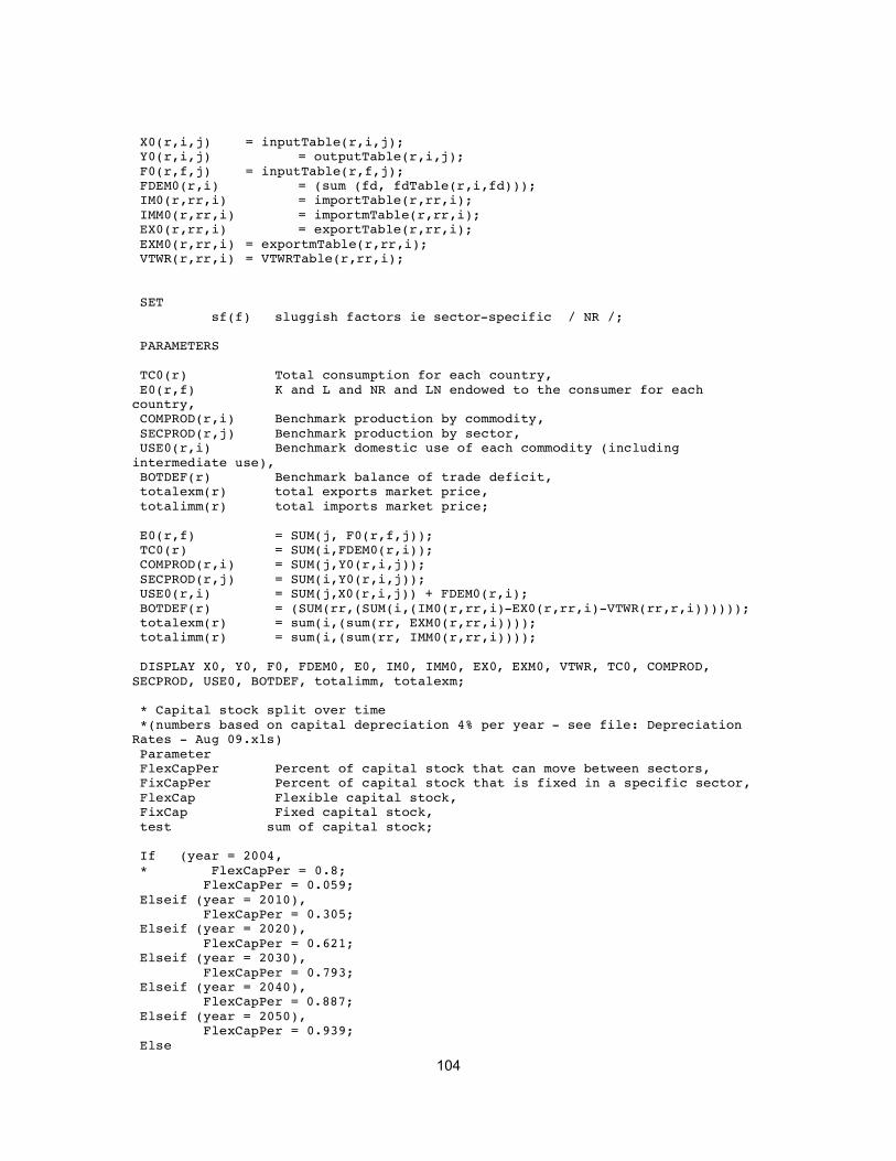
104

! ! !X0(r,i,j) = inputTable(r,i,j); !Y0(r,i,j) = outputTable(r,i,j); !F0(r,f,j) = inputTable(r,f,j); !FDEM0(r,i) = (sum (fd, fdTable(r,i,fd))); !IM0(r,rr,i) = importTable(r,rr,i); !IMM0(r,rr,i) = importmTable(r,rr,i); !EX0(r,rr,i) = exportTable(r,rr,i); !EXM0(r,rr,i) = exportmTable(r,rr,i); !VTWR(r,rr,i) = VTWRTable(r,rr,i); ! ! !SET ! sf(f) sluggish factors ie sector-specific / NR /; ! !PARAMETERS ! !TC0(r) Total consumption for each country, !E0(r,f) K and L and NR and LN endowed to the consumer for each country, !COMPROD(r,i) Benchmark production by commodity, !SECPROD(r,j) Benchmark production by sector, !USE0(r,i) Benchmark domestic use of each commodity (including intermediate use), !BOTDEF(r) Benchmark balance of trade deficit, !totalexm(r) total exports market price, !totalimm(r) total imports market price; ! !E0(r,f) = SUM(j, F0(r,f,j)); !TC0(r) = SUM(i,FDEM0(r,i)); !COMPROD(r,i) = SUM(j,Y0(r,i,j)); !SECPROD(r,j) = SUM(i,Y0(r,i,j)); !USE0(r,i) = SUM(j,X0(r,i,j)) + FDEM0(r,i); !BOTDEF(r) = (SUM(rr,(SUM(i,(IM0(r,rr,i)-EX0(r,rr,i)-VTWR(rr,r,i)))))); !totalexm(r) = sum(i,(sum(rr, EXM0(r,rr,i)))); !totalimm(r) = sum(i,(sum(rr, IMM0(r,rr,i)))); ! !DISPLAY X0, Y0, F0, FDEM0, E0, IM0, IMM0, EX0, EXM0, VTWR, TC0, COMPROD, SECPROD, USE0, BOTDEF, totalimm, totalexm; !! !* Capital stock split over time !*(numbers based on capital depreciation 4% per year - see file: Depreciation Rates - Aug 09.xls) !Parameter !FlexCapPer Percent of capital stock that can move between sectors, !FixCapPer Percent of capital stock that is fixed in a specific sector, !FlexCap Flexible capital stock, !FixCap Fixed capital stock, !test sum of capital stock; ! !If (year = 2004, !* FlexCapPer = 0.8; ! FlexCapPer = 0.059; !Elseif (year = 2010), ! FlexCapPer = 0.305; !Elseif (year = 2020), ! FlexCapPer = 0.621; !Elseif (year = 2030), ! FlexCapPer = 0.793; !Elseif (year = 2040), ! FlexCapPer = 0.887; !Elseif (year = 2050), ! FlexCapPer = 0.939; !Else

105

! abort "error with year value"; !); ! ! !FixCapPer = (1-FlexCapPer); !FlexCap(r) = sum(j,(F0(r,"K",j)*FlexCapPer)); !FixCap(r,j) = F0(r,"K",j)*FixCapPer; ! ! !Display FlexCap, FixCap, test, E0, FlexCapPer, FixCapPer; ! ! !* Carbon Accounting Sector ! !SET !* We treat oil as a material feedstock for all sectors (i.e. oil is non emitting) ! e(i) energy goods only / ELEC, GAS, COAL, RPP/, ! fe(i) final energy goods that emit carbon only / COAL, GAS, RPP /, ! lfe(i) liquid final energy goods that emit carbon only / GAS, RPP /, ! ne(i) non energy goods only / OIL, MET, NMET, OMAN, TRANS, ROE/, ! nce(i) non carbon emitting goods only / OIL, MET, NMET, OMAN, TRANS, ROE, ELEC/, ! ele(i) electricity only / ELEC /; ! !ALIAS (fe,ff); ! !PARAMETERS ! ! CARB_INT_GJ(r,fe) Emission of CO2 in tonnes per GJ of fuel consumed, ! FUEL_PJ0(r,fe) Consumption of fuel in PJ, ! CO2EMIT0(r,fe) Benchmark total CO2 emission by fuel in MT, ! CARBONCOEF(r,fe) Emission of CO2 by fuel in MT per dollar, ! TOTALCARB0(r) Benchmark total CO2 emissions in MT, ! SECTORCARB0(r,j) Benchmark sector CO2 emission in MT, ! HOUSECARB(r) Benchmark household CO2 emission in MT, ! ABATE(r) Percentage of total emissions to be reduced, ! GLOBALABATE Percentage of global emissions to be reduced; ! !ABATE(r)$(opt=2) = 0; !GLOBALABATE$(opt=1) = 0; ! !* CO2 intesity for each fuel (these are from file: Carbon Content of fossil fuels 2009.xls ) I calculated values form EIA CO2 intensities !CARB_INT_GJ("US","COAL") = 0.09240; !CARB_INT_GJ ("US","GAS") = 0.05029; !CARB_INT_GJ ("US","RPP") = 0.06883; ! !*These are based on the IPCC values for calcualting emissions !CARB_INT_GJ("ROW","COAL") = 0.0901; !CARB_INT_GJ ("ROW","GAS") = 0.0513; !CARB_INT_GJ ("ROW","RPP") = 0.0718; ! !*Fuel Forecast !*1st line of US fuel #s are from 2004 EIA historical records - consumption of fuel by source !*1st line of ROW fuel #s are from 2004 EIA - International energy annual - historical records - consumption of fuel by source !*numbers from 2010 - 2050 from EIA and IEO see file: Energy Data Forecasts Aug 2009.xls - I am concerned about RPP numbers - they are total RPP - not just combustible ones ! !If (year = 2004,

106

! FUEL_PJ0("US","COAL") = 23848.4129; FUEL_PJ0("US","GAS") = 24193.9932; FUEL_PJ0("US","RPP") = 42512.7909; ! FUEL_PJ0("ROW","COAL")= 98064.69402; FUEL_PJ0("ROW","GAS")= 84757.39354; FUEL_PJ0("ROW","RPP") = 133364.8097; ! !Elseif (year = 2010), ! FUEL_PJ0("US","COAL") = 23447.81983; FUEL_PJ0("US","GAS") = 23822.03281; FUEL_PJ0("US","RPP") = 39176.62979; ! FUEL_PJ0("ROW","COAL")= 124893.033; FUEL_PJ0("ROW","GAS")= 101202.0857; FUEL_PJ0("ROW","RPP") = 145141.6277; ! !Elseif (year = 2020), ! FUEL_PJ0("US","COAL") = 25663.75749; FUEL_PJ0("US","GAS") = 23357.8506; FUEL_PJ0("US","RPP") = 38636.86231; ! FUEL_PJ0("ROW","COAL")= 144938.7739; FUEL_PJ0("ROW","GAS")= 126143.5637; FUEL_PJ0("ROW","RPP") = 166254.9843; ! !Elseif (year = 2030), ! FUEL_PJ0("US","COAL") = 26577.75836; FUEL_PJ0("US","GAS") = 25486.72554; FUEL_PJ0("US","RPP") = 39036.01752; ! FUEL_PJ0("ROW","COAL")= 174093.8648; FUEL_PJ0("ROW","GAS")= 141212.0992; FUEL_PJ0("ROW","RPP") = 188539.5299; ! !Elseif (year = 2040), ! FUEL_PJ0("US","COAL") = 27799.22816; FUEL_PJ0("US","GAS") = 28399.8669; FUEL_PJ0("US","RPP") = 39721.01343; ! FUEL_PJ0("ROW","COAL")= 197096.4774; FUEL_PJ0("ROW","GAS")= 162701.127; FUEL_PJ0("ROW","RPP") = 210478.6796; ! !Elseif (year = 2050), ! FUEL_PJ0("US","COAL") = 28950.46951; FUEL_PJ0("US","GAS") = 30821.37895; FUEL_PJ0("US","RPP") = 40357.32044; ! FUEL_PJ0("ROW","COAL")= 222047.3178; FUEL_PJ0("ROW","GAS")= 182121.9522; FUEL_PJ0("ROW","RPP") = 232599.2338; ! !!Else ! abort "error with year and fuel value"; !); ! !*Emission of CO2 if there is a carbon intensity value (if it actually emits carbon) !CO2EMIT0(r,fe)$CARB_INT_GJ(r,fe) = FUEL_PJ0(r,fe) * CARB_INT_GJ(r,fe); !CARBONCOEF(r,fe)$USE0(r,fe) = CO2EMIT0(r,fe) /USE0(r,fe); ! !TOTALCARB0(r) = SUM(fe, CO2EMIT0(r,fe)); !SECTORCARB0(r,j) = SUM(fe, X0(r,fe,j) * CARBONCOEF(r,fe)); !HOUSECARB(r) = SUM(fe, FDEM0(r,fe) * CARBONCOEF(r,fe)); ! !*Alternative sector for CCS !SET ! !s Steps for CCS sector /1,2,3/, !q Quantity of capacity for CCS sector /q/; ! !!PARAMETER ! !ATechf(r,j,s,f) Factor adjustment data for alternative CCS sector, !ATechfe(r,j,s,fe) Fuel (carbon emitting) adjustment data for alternative CCS sector, !ATechq(r,j,s) Quantity of alternative CCS sector available, !ATechcs(r,j,s) Carbon sequestion (percent of fuel used that is sequestered), !altsec(r,j) CCS sector indicator, ! !CS0(r,j,s) Carbon sequestration,

107

!XA0(r,j,s,i) Benchmark fuel inputs to CCS sector, !YA0(r,j,s,i) Benchmark output from alternate sector, !FA0(r,j,s,f) Benchmark factors for CCS sector, !EA0(r,j,s) Endowments of capacity for CCS sector, !ASECPROD(r,j,s) secprod with (s); ! !altsec(r,j) =0; !altsec(r,"ELECJ") =1; ! !ATechf("ROW",j,s,f) = ROWATech(j,s,f); !ATechf("US",j,s,f) = USATech(j,s,f); ! !ATechfe("ROW",j,s,fe) = ROWATech(j,s,fe); !ATechfe("US",j,s,fe) = USATech(j,s,fe); ! !ATechq ("US",j,s) = USATech(j,s,"Q"); !ATechq("ROW",j,s) = ROWATech(j,s,"Q"); ! !ATechcs("ROW", j, s) = ROWATech(j,s,"CS"); !Atechcs("US", j, s) = USATech(j,s,"CS"); ! ! !XA0(r,j,s,fe)$altsec(r,j) = (X0(r,fe,j)* (ATechfe(r,j,s,fe))*Atechq(r,j,s)); !XA0(r,j,s,i)$altsec(r,j) = (X0(r,i,j)*Atechq(r,j,s)); !Sumxao(r,j) = sum(fe,(sum(s,(xa0(r,j,s,fe))))); !YA0(r,j,s,i)$altsec(r,j) = (Y0(r,i,j) * (ATechq(r,j,s))); !ASECPROD(r,j,s)$altsec(r,j) = sum(i,YA0(r,j,s,i)$altsec(r,j)); !FA0(r,j,s,f)$altsec(r,j) = (F0(r,f,j) * (1+Atechf(r,j,s,f))*Atechq(r,j,s)); !FA0(r,j,s,"LN")$altsec(r,j) = (Atechf(r,j,s,"LN")*YA0(r,"ELECJ","3","ELEC")); ! !EA0(r,j,s)$altsec(r,j) = (SECPROD(r,j) * Atechq(r,j,s)); !CS0(r,j,s)$altsec(r,j) = (sum(fe,(CARBONCOEF(r,fe)*(XA0(r,j,s,fe)))* ATechcs(r,j,s))); !CS0(r,j,"3")$altsec(r,j) = (Atechcs(r,j,"3") * YA0(r,"ELECJ","3","ELEC")); ! ! !*Revenue recycling !PARAMETER PR(r,j) Percentage of carbon tax revenue recycled to sectors instead of being given to households; ! !PR(r,j) = 0; ! !*International fund transfer - for use in regional mode to transfer money from US to ROW !PARAMETER PT percent for interntation fund transfer; !PT$(opt=2) = 0; ! ! !*Permit allocation to different regions - use to allocate permit value to different regions in global mode !PARAMETER allo allocation of revenue to regions ; ! !allo("US")$(opt=1) = (TOTALCARB0("US")/(sum(r, TOTALCARB0(r)))); !allo("ROW")$(opt=1) = (1 - allo("US")) ; ! ! !*Load elasticities of substitution !$INCLUDE Elas_US_ROW Nov 12.txt ! !

108

!Display CO2EMIT0,FUEL_PJ0, CARB_INT_GJ, FUEL_PJ0, esub_s, esub_ii, esub_vae, esub_va, esub_cva, esub_slug, esub_mob, esub_e, esub_fuel, esub_lqd, edem_s, edem_c, edem_e, edem_hou, esub_domex , esub_arm; ! ! *MPSGE section !$ONTEXT !$MODEL:TRADE ! !$SECTORS: ! !Y(r,j) !Production from each sector from flexible capital !X(r,j)$FixCap(r,j) !Production from each sector from fixed capital !Ya(r,j,s)$altsec(r,j) !Alternative production of Electricity (CCS) !CARB(r,fe) !Production of carbon taxed energy commodities !AR(r,i) !Armington aggregator for each commodity !DOMEX(r,i) !Domestic production for export or Armington !C(r) !Consumption aggregate !IMP(r,rr,i)$IM0(r,rr,i) !Domestic import transformation sector ! !$COMMODITIES: ! !PY(r,i) !Price index for each commodity !PLab(r) !Price index for Labour !PflK(r) !Price index for flexible capital !PLN(r)$E0(r,"LN") !Price index for land !PfixK(r,j)$FixCap(r,j) !Price index for fixed capital (sector-specific) ie. indexed over j !PSF(r,sf,j)$F0(r,sf,j) !Price index for natural resources (sector-specific) ie. indexed over j !PA(r,i) !Price index for Armington good !PC(r) !Price index for aggregate consumption !PD(r,i) !Price index for production for domestic consumption !PX(r,rr,i)$EX0(r,rr,i) !Price index for exports !PM(r,rr,i)$IM0(r,rr,i) !Price index for imports !PAC(r,fe) !Price index for Armington goods with a carbon permit !PCARB(r)$(ABATE(r) AND (opt=2)) !Price index of carbon permits !PCARBGLOBE$(GLOBALABATE AND (opt=1)) !Price index of carbon permits for the globe !PQ(r,j,s)$altsec(r,j) !Price index for capacity at alternative steps ! !$AUXILIARY: ! !LS(r,j)$(ABATE(r) and PR(r,j)) !Output subsidy transfer rate for region r, sector j for regional permit method !LS(r,j)$(GLOBALABATE and PR(r,j)) !Output subsidy transfer rate region r, sector j for global permit method !*TRN("US")$(PT AND ABATE("US")) !Percent of of perimt revenue transfered to international - Lump sum transfer of PC !TRN$(PT) !Percent of of perimt revenue transfered to international - Lump sum transfer of PC ! ! !$CONSUMERS: ! !CON(r) !Representative agent !

109

!$PROD:Y(r,j) S:ESUB_S(r,j) vae(s):ESUB_VAE(r,j) ii(s):ESUB_II(r,j) va(vae):ESUB_VA(r,j) e(vae):ESUB_E(r,j) slug(va):ESUB_SLUG(r,j) mob(va):ESUB_MOB(r,j) fuel(e):ESUB_FUEL(r,j) lqd(fuel):ESUB_LQD(r,j) ! ! I:PLab(r) Q:F0(r,"L",j) mob: ! I:PflK(r) Q:F0(r,"K",j) mob: ! I:PLN(r) Q:F0(r,"LN",j) slug: !` I:PSF(r,sf,j) Q:F0(r,sf,j) slug: ! I:PA(r,nce) Q:X0(r,nce,j) ii:$(not e(nce)) e:$ele(nce) ! I:PAC(r,"coal") Q:X0(r,"coal",j) fuel: ! I:PAC(r,lfe) Q:X0(r,lfe,j) lqd: ! O:PY(r,i)$(opt=2) Q:Y0(r,i,j) A:CON(r) N:LS(r,j)$(ABATE(r) AND PR(r,j)) M:(-1)$(ABATE(r) AND PR(r,j)) ! O:PY(r,i)$(opt=1) Q:Y0(r,i,j) A:CON(r) N:LS(r,j)$(GLOBALABATE AND PR(r,j)) M:(-1)$(GLOBALABATE AND PR(r,j)) ! ! !$PROD:X(r,j)$FixCap(r,j) s:0 ! ! I:PLab(r) Q:F0(r,"L",j) ! I:PfixK(r,j) Q:F0(r,"K",j) ! I:PLN(r) Q:F0(r,"LN",j) !` I:PSF(r,sf,j) Q:F0(r,sf,j) ! I:PA(r,nce) Q:X0(r,nce,j) ! I:PAC(r,"coal") Q:X0(r,"coal",j) ! I:PAC(r,lfe) Q:X0(r,lfe,j) ! O:PY(r,i)$(opt=2) Q:Y0(r,i,j) A:CON(r) N:LS(r,j)$(ABATE(r) AND PR(r,j)) M:(-1)$(ABATE(r) AND PR(r,j)) ! O:PY(r,i)$(opt=1) Q:Y0(r,i,j) A:CON(r) N:LS(r,j)$(GLOBALABATE AND PR(r,j)) M:(-1)$(GLOBALABATE AND PR(r,j)) ! !$PROD:Ya(r,j,s)$altsec(r,j) cs1:0 cs(cs1):0 cvae(s):0 cva(cvae):ESUB_CVA(r,"ELECJ") ce(cvae):ESUB_E(r,j) cslu(cva):0 cmob(cva):0 cfue(ce):ESUB_FUEL(r,j) clqd(cfue):ESUB_LQD(r,j) T:0 ! ! I:PLab(r) Q:FA0(r,j,s,"L") cmob: ! I:PflK(r) Q:FA0(r,j,s,"K") cmob: ! I:PLN(r) Q:FA0(r,j,s,"LN") cslu: !` I:PSF(r,sf,j) Q:FA0(r,j,s,sf) cslu: ! I:PA(r,ele) Q:XA0(r,j,s,ele) ce: ! I:PA(r,ne) Q:XA0(r,j,s,ne) cs1: ! I:PAC(r,"COAL") Q:XA0(r,j,s,"COAL") cfue: ! I:PAC(r,lfe) Q:XA0(r,j,s,lfe) clqd: ! I:PQ(r,j,s)$altsec(r,j) Q:ASECPROD(r,j,s) ! O:PY(r,i) Q:YA0(r,j,s,i) ! O:PCARB(r)$(ABATE(r) AND (opt=2)) Q:CS0(r,j,s) ! O:PCARBGLOBE$(GLOBALABATE AND (opt=1)) Q:CS0(r,j,s) ! !$PROD:CARB(r,fe) s:0 ! ! I:PA(r,fe) Q:USE0(r,fe) ! I:PCARB(r)$(ABATE(r) AND (opt=2)) Q:((CARBONCOEF(r,fe)*USE0(r,fe))) ! I:PCARBGLOBE$(GLOBALABATE AND (opt=1)) Q:((CARBONCOEF(r,fe)*USE0(r,fe))) ! O:PAC(r,fe) Q:USE0(r,fe) ! !$PROD:DOMEX(r,i) T:ESUB_DOMEX(r,i) ! ! I:PY(r,i) Q:COMPROD(r,i) ! O:PX(r,rr,i)$EXM0(r,rr,i) Q:EXM0(r,rr,i) ! O:PD(r,i) Q:(COMPROD(r,i)-(sum(rr,EXM0(r,rr,i)))) ! !$PROD:IMP(r,rr,i)$IM0(r,rr,i)

110

! ! I:PX(rr,r,i)$EX0(rr,r,i) Q:(EX0(rr,r,i)+ VTWR(r,rr,i)) ! O:PM(r,rr,i) Q:IM0(r,rr,i) ! !$PROD:AR(r,i)$USE0(r,i) S:ESUB_ARM(r,i) ! ! I:PD(r,i) Q:(COMPROD(r,i)-(sum(rr,EXM0(r,rr,i)))) ! I:PM(r,rr,i) Q:IMM0(r,rr,i) ! O:PA(r,i) Q:(COMPROD(r,i)-(sum(rr,EXM0(r,rr,i))) + (sum(rr,IMM0(r,rr,i)))) ! !$PROD:C(r) S:EDEM_S(r) c(S):EDEM_C(r) e(S):EDEM_E(r) hou(e):EDEM_HOU(r) ! ! I:PA(r,nce) Q:FDEM0(r,nce) c:$(not e(nce)) hou:$ele(nce) ! I:PAC(r,"coal") Q:FDEM0(r,"coal") e: ! I:PAC(r,"gas") Q:FDEM0(r,"gas") hou: ! I:PAC(r,"rpp") Q:FDEM0(r,"rpp") e: ! O:PC(r) Q:TC0(r) ! ! ! !$DEMAND: CON(r) ! ! D:PC(r) Q:(TC0(r)) ! E:PLab(r) Q:E0(r,"L") E:PflK(r)$E0(r,"K") Q:FlexCap(r) ! E:PfixK(r,j) Q:FixCap(r,j) ! E:PSF(r,sf,j)$F0(r,"NR",j) Q:F0(r,"NR",j) ! E:PLN(r)$E0(r,"LN") Q:E0(r,"LN") ! E:PX(r,rr,i) Q:((-1)*((EXM0(r,rr,i)-EX0(r,rr,i)- VTWR(rr,r,i)))) ! E:PM(r,rr,i) Q:(IMM0(r,rr,i)-IM0(r,rr,i)) ! E:PCARBGLOBE$(GLOBALABATE AND (opt=1)) Q:((1-GLOBALABATE)*(SUM(rr,(SUM(fe,(CARBONCOEF(rr,fe)*USE0(rr,fe))))))*allo(r)) ! E:PCARB(r)$(ABATE(r) AND (opt=2)) Q:((1-ABATE(r))*(sum(fe,(CARBONCOEF(r,fe)*USE0(r,fe))))) ! E:PC("US")$(BOTDEF(r)) Q:(BOTDEF(r)) ! E:PQ(r,j,s)$altsec(r,j) Q:(EA0(r,j,s)) ! E:PC("US")$(PT) Q:(-1) R:TRN ! E:PC("ROW")$(PT) Q:1 R:TRN ! ! !$REPORT: ! V:TotalFuelDemand(r,fe) O:PAC(r,fe) PROD:CARB(r,fe) ! V:NumberofGlobalPermits(r,fe)$(opt=1) I:PCARBGLOBE PROD:CARB(r,fe) ! V:Imports(r,rr,i) O:PM(r,rr,i) PROD:IMP(r,rr,i) ! V:Exports(r,rr,i) O:PX(r,rr,i) PROD:DOMEX(r,i) ! V:FlexCapDem(r,j) I:PflK(r) PROD:Y(r,j) ! V:FlexCapDemYa(r,j,s)$altsec(r,j) I:PflK(r) PROD:Ya(r,j,s) ! V:FixCapDemX(r,j)$FixCap(r,j) I:PfixK(r,j) PROD:X(r,j) ! V:FacDemS(r,sf,j) I:PSF(r,sf,j) PROD:Y(r,j) ! V:FacDemSX(r,sf,j) I:PSF(r,sf,j) PROD:X(r,j) ! V:FacDemSYa(r,sf,j,s)$altsec(r,j) I:PSF(r,sf,j) PROD:Ya(r,j,s) ! V:FinDem(r,nce) I:PA(r,nce) PROD:C(r) ! V:FinDemCarb(r,fe) I:PAC(r,fe) PROD:C(r) ! V:LabDem(r,j) I:PLab(r) PROD:Y(r,j) ! V:LabDemYa(r,j,s)$altsec(r,j) I:PLab(r) PROD:Ya(r,j,s) ! V:LabDemX(r,j) I:PLab(r) PROD:X(r,j) ! V:LNDem(r,j) I:PLN(r) PROD:Y(r,j) ! V:LNDemX(r,j) I:PLN(r) PROD:X(r,j) ! V:LNDemYa(r,j,s)$altsec(r,j) I:PLN(r) PROD:Ya(r,j,s) ! V:Qij(r,i,j) O:PY(r,i) PROD:Y(r,j)

111

! V:QijX(r,i,j) O:PY(r,i) PROD:X(r,j) ! V:QijYa(r,i,j,s)$altsec(r,j) O:PY(r,i) PROD:Ya(r,j,s) ! V:Capacity(r,j,s)$altsec(r,j) I:PQ(r,j,s) PROD:Ya(r,j,s) ! V:SectorFuelUse(r,fe,j) I:PAC(r,fe) PROD:Y(r,j) ! V:SectorFuelUseX(r,fe,j) I:PAC(r,fe) PROD:X(r,j) ! V:SectorFuelUseYa(r,fe,j,s)$altsec(r,j) I:PAC(r,fe) PROD:Ya(r,j,s) ! V:SectorPAUseY(r,nce,j) I:PA(r,nce) PROD:Y(r,j) ! V:SectorPAUseX(r,nce,j) I:PA(r,nce) PROD:X(r,j) ! V:SectorPAUseYa(r,nce,j,s)$altsec(r,j) I:PA(r,nce) PROD:Ya(r,j,s) ! V:SectorPCarb(r,j,s)$(opt=2) O:PCARB(r) PROD:Ya(r,j,s) ! V:SectorPCarbGlobe(r,j,s)$(opt=1) O:PCARBGLOBE PROD:Ya(r,j,s) ! V:EqVar(r) W:CON(r) !* EqVar - similar to consumer surplus ! !$CONSTRAINT: TRN$(PT) !TRN*PC("US") =e= PCARB("US")*(1-ABATE("US"))*(SUM(fe,(CARBONCOEF("US",fe)*USE0("US",fe))))*PT; !! !* Application of an output subsidy as a tax rate. It is divided by total output in order to get a RATE, which is applied to the output of the sector. !*In both LS equations, both sides are divided by PC, so they cancel out. In the policy file the PC is retained in the term with secprod and asecprod. !$CONSTRAINT: LS(r,j)$(ABATE(r) AND PR(r,j)) !LS(r,j)*(sum(i,((((Y(r,j)+ X(r,j))*SECPROD(r,j))+(sum(s,(Ya(r,j,s)$altsec(r,j)*ASECPROD(r,j,s)))))*PY(r,i))))=e= PCARB(r)*PR(r,j)*((1-ABATE(r)))*(SUM(fe,(CARBONCOEF(r,fe)*USE0(r,fe)))); ! ! !$CONSTRAINT: LS(r,j)$(GLOBALABATE AND PR(r,j)) !LS(r,j)*(sum(i,(((((Y(r,j)+ X(r,j))*SECPROD(r,j)) +(sum(s,(Ya(r,j,s)$altsec(r,j)*ASECPROD(r,j,s)))))*PY(r,i)))))=e= PCARBGLOBE*(SUM(rr,(SUM(fe,(CARBONCOEF(rr,fe)*USE0(rr,fe))))))*(1-GLOBALABATE)*allo(r)*PR(r,j); !! !$OFFTEXT ! !$SYSINCLUDE MPSGESET TRADE !! !* set Numeraire !PLab.FX ("US") = 1 ; ! !*This statement imposes a lower bound on industry output in the counterfactual (hopefully prevents LS(r,j) from crashing) !Y.LO(r,j) = 0.001; ! !*Include policy file !$INCLUDE "globalpoliciesDec3.gms" ; ! ! !

112

Appendix B: Set j - Sectors in VERITAS-US

Sector Description of Sectoral Activities

OILJ Crude Oil: Extraction of crude petroleum

ELECJ Electricity: electricity production and distribution

GASJ Natural Gas: gas extraction, manufacture and distribution

COALJ Coal: coal mining and agglomeration

RPPJ Refined Petroleum Products: refined petroleum products and coke

METJ Metal Industry: metal mining and manufacture (minerals, ferrous metals, other metals, metal products)

NMETJ Non-Mental Industry: wood products, paper products and publishing, chemical, rubber, plastic products, non-metal mineral products

OMANJ

Other Manufacture: food and beverage manufacture and processing, textile, leather and clothing manufacture, motor vehicle parts and transportation equipment, electronics, machinery and equipment, other manufacture

TRANJ Transportation: sea, air and other transport

ROEJ

Rest of Economy: trade, insurance, communication, financial services, business services, recreation, public administration, defence, health, education, dwellings, construction, water, fishing, forestry, agriculture (producing raw products)

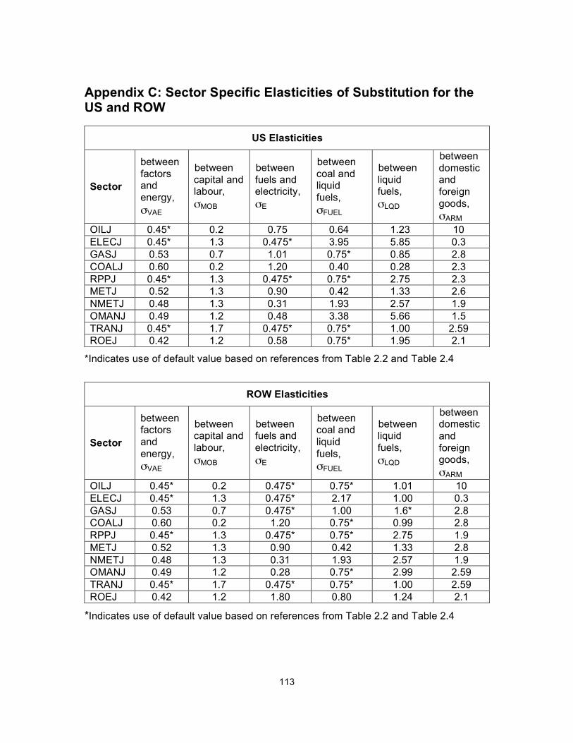
113

Appendix C: Sector Specific Elasticities of Substitution for the US and ROW

US Elasticities

Sector

between factors and energy, !VAE

between capital and labour, !MOB

between fuels and electricity, !E

between coal and liquid fuels, !FUEL

between liquid fuels, !LQD

between domestic and foreign goods, !ARM

OILJ 0.45* 0.2 0.75 0.64 1.23 10 ELECJ 0.45* 1.3 0.475* 3.95 5.85 0.3 GASJ 0.53 0.7 1.01 0.75* 0.85 2.8 COALJ 0.60 0.2 1.20 0.40 0.28 2.3 RPPJ 0.45* 1.3 0.475* 0.75* 2.75 2.3 METJ 0.52 1.3 0.90 0.42 1.33 2.6 NMETJ 0.48 1.3 0.31 1.93 2.57 1.9 OMANJ 0.49 1.2 0.48 3.38 5.66 1.5 TRANJ 0.45* 1.7 0.475* 0.75* 1.00 2.59 ROEJ 0.42 1.2 0.58 0.75* 1.95 2.1

*Indicates use of default value based on references from Table 2.2 and Table 2.4

ROW Elasticities

Sector

between factors and energy, !VAE

between capital and labour, !MOB

between fuels and electricity, !E

between coal and liquid fuels, !FUEL

between liquid fuels, !LQD

between domestic and foreign goods, !ARM

OILJ 0.45* 0.2 0.475* 0.75* 1.01 10 ELECJ 0.45* 1.3 0.475* 2.17 1.00 0.3 GASJ 0.53 0.7 0.475* 1.00 1.6* 2.8 COALJ 0.60 0.2 1.20 0.75* 0.99 2.8 RPPJ 0.45* 1.3 0.475* 0.75* 2.75 1.9 METJ 0.52 1.3 0.90 0.42 1.33 2.8 NMETJ 0.48 1.3 0.31 1.93 2.57 1.9 OMANJ 0.49 1.2 0.28 0.75* 2.99 2.59 TRANJ 0.45* 1.7 0.475* 0.75* 1.00 2.59 ROEJ 0.42 1.2 1.80 0.80 1.24 2.1

*Indicates use of default value based on references from Table 2.2 and Table 2.4

114

REFERENCE LIST

Works Cited

Al-Juaied, M., Whitmore, A., 2009. Realistic Costs of Carbon Capture. Belfer Center for Science and International Affairs, Discussion Paper 2009-08, Cambridge, MA.

Allison, I., Bindoff, N.L., Bindschadler, R.A., Cox, P.M., de Noblet, N., England, M.H., Francis, J.E., Gruber, N., Haywood, A.M., Karoly, D.J., Kaser, G., Le Quéré, C., Lenton, T.M., Mann, M.E., McNeil, B.I., Pitman, A.J., Rahmstorf, S., Rignot, E., Schellnhuber, H.J., Schneider, S.H., Sherwood, S.C., Somerville, R.C.J., Steffen, K., Steig, E.J., Visbeck, M., Weaver, A.J., 2009. The Copenhagen Diagnosis: Updating the World on the Latest Climate Science. The University of New South Wales Climate Change Research Centre (CCRC), Sydney, Australia.

Armington, P.S., 1969. A Theory of Demand for Products Distinguished by Place of Production. International Monetary Fund, Staff Papers 16,159-178.

Azar, C., Dowlatabadi, H., 1999. A Review of Technical Change in Assessment of Climate Policy. Annual Review of Energy and the Environment 24, 513-544.

Babiker, M.H., Maskus, K.E., Rutherford, T.F., 1997. Carbon Taxes and the Global Trading System. Working Paper 97-7, University of Colorado, Boulder.

Babiker, M.H., Metcalf, G.E., Reilly, J., 2003. Tax distortions and global climate policy. Journal of Environmental Economics and Management 46, 269-287.

Babiker, M.H., Reilly, J.M., Mayer, M., Eckaus, R.S., Sue Wing, I., Hyman,

R.C., 2001. The MIT Emissions Prediction and Policy Analysis (EPPA) Model: Revisions, Sensitivities, and Comparisons of Results. MIT Joint Program on the Science and Policy of Global Change Report 71, Cambridge, MA.

Badri, N.G., Walmsley, T.L., (Eds.), 2008. Global Trade, Assistance, and Production: The GTAP 7 Data Base, Chapter 14: Behavioural Parameters. Centre for Global Trade Analysis, Purdue University.

115

Bataille, C., 2005. Design and Application of a Technologically Explicit Hybrid Energy-Economy Model with Micro and Macro Economic Dynamics. PhD Thesis, Simon Fraser University.

Bataille, C., Jaccard, M., Nyboer, J., Rivers, N., 2006. Towards General Equilibrium in a Technology-Rich Model with Empirically Estimated Behavioral Parameters. The Energy Journal 27, 93-112.

Bernard, A.L., Fischer, C., Fox, A.K., 2007. Is there a rationale for output-based rebating of environmental levies? Resource and Energy Economics 29, 83-101.

Böhringer, C., 1998. The synthesis of bottom-up and top-down in energy policy modeling. Energy Economics 20, 233-248.

Böhringer, C., Rutherford, T.F., 2001. World Economic Impacts of the Kyoto Protocol. In: Welfens, P.J.J. (Ed.), Internationalization of the Economy and Environmental Policy Options. Springer, New York, pp. 161-178.

Böhringer, C., Rutherford, T.F., 2002. Carbon Abatement and International Spillovers. Environmental and Resource Economics 22, 391-417.

Boyce, J.K., Riddle, M., 2007. Cap and Dividend: How to Curb Global Warming While Protecting the Incomes of American Families. PERI Working Paper, Series Number 150.

Burniaux, J.M., Truong, P., 2002. GTAP-E: An Energy-Environmental Version of

the GTAP Model. Center for Global Trade Analysis, GTAP Technical Paper No. 16. Purdue University.

Burtraw, D., Sweeney, R., Walls, M.A., 2009. The Incidence of U.S. Climate

Policy: Alternative Uses of Revenues from a Cap-and-Trade Auction. Resources for the Future, Discussion Paper 09-17-REV. Washington, DC.

Center for Global Trade Analysis, 2001. Global Trade, Assistance and Production: The Constrained GTAP7 Data Package, CD-ROM, Purdue University.

Energy Information Administration, 2008. International Energy Annual 2006. U.S. Department of Energy, Washington, DC. Table 1.8 World Consumption of Primary Energy by Energy Type, 1980-2006. Retrieved July 2009, from http://www.eia.doe.gov/iea/wecbtu.html

Energy Information Administration, 2009a. International Energy Outlook 2009. Chapter 1: World Energy Demand and Economic Outlook. Report #:DOE/EIA-0484(2009), U.S. Department of Energy, Washington, DC. Retrieved July 2009, from http://www.eia.doe.gov/oiaf/ieo/

116

Energy Information Administration, 2009b. Annual Energy Review 2008. Report #:DOE/EIA-0384(2008), U.S. Department of Energy, Washington, DC. Table 1.3 Primary Energy Consumption by Source, 1949-2008. Retrieved July 2009, from <http://www.eia.doe.gov/emeu/aer/overview.html

Energy Information Administration, 2009c. Updated Annual Energy Outlook 2009 Reference Case. Report #: SR-OIAF/2009-03, U.S. Department of Energy, Washington, DC. Table 1 Total Energy supply and disposition and Table 2 Energy Consumption by Sector and Source. Retrieved July 2009, from http://www.eia.doe.gov/oiaf/servicerpt/stimulus/aeostim.html

Energy Information Administration, 2009d. International Energy Outlook 2009. Report #:DOE/EIA-0484(2009), U.S. Department of Energy, Washington, DC. Table A2 World Total Energy Consumption by Region and Fuel. Retrieved July 2009, from http://www.eia.doe.gov/oiaf/ieo/ieorefcase.html

Energy Information Administration, 2009e. The National Energy Modeling System: An Overview. Report #:DOE/EIA-0581(2009), U.S. Department of Energy, Washington, DC. Retrieved February 2010, from http://www.eia.doe.gov/oiaf/aeo/overview/

Energy Information Administration, 2009f. Energy Market and Economic Impacts of H.R. 2454, the American Clean Energy and Security Act of 2009. Report #: SR/OIAF/2009-05, U.S. Department of Energy, Washington, DC.

Environmental Protection Agency, 2009. EPA Analysis of the American Clean Energy and Security Act of 2009 H.R. 2454 in the 111th Congress. Office of Atmospheric Programs. Retrieved September 2009, from www.epa.gov/climatechange/economics/ economicanalyses.html

Fischer, C., 2001. Rebating Environmental Policy Revenues: Output-Based Allocations and Tradable Performance Standards. Resources for the Future, Discussion Paper 01–22. Washington, DC.

Fischer, C., Fox, A.K., 2009. Combining Rebates with Carbon Taxes: Optimal Strategies for Coping with Emission Leakage and Tax Interactions. Resources for the Future, Discussion Paper 09–12. Washington, DC.

Fofana, I., Lemelin, A., Cockburn, J., 2002. Balancing a Social Accounting Matrix. Centre de Recherche en Économie et Finances Appliquées (CREFA), Université Laval.

Gallaway, M.P., McDaniel, C.A., Rivera, S.A., 2003. Short-run and long-run industry-level estimates of U.S. Armington elasticities. The North American Journal of Economics and Finance 14, 49-68.

Goulder, L.H., 1995. Evnironmental Taxation and the Double Dividend: A Reader’s Guide. International Tax and Public Finance 2, 157-183.

117

Grubb, M., Köhler, J., Anderson, D., 2002. Induced technical Change in Energy and Environmental Modelling: Analytic Approaches and Policy Implications. Annual Review of Energy and the Environment 27, 271-308.

Hourcade, J., Jaccard, M., Bataille, C., Ghersi, F., 2006. Hybrid Modeling: New Answers to Old Challenges Introduction to the Special Issue of The Energy Journal. Energy Journal 27, 1-11.

International Energy Agency, 2006. IEA Energy Technology Essentials: CO2 Capture & Storage. ETE01. Retrieved August 2009, from www.iea.org/Textbase/techno/essentials.htm

International Energy Agency, 2009. Carbon Capture and Storage: Full-scale Demonstration Progress Update. Retrieved December 2009, from http://www.iea.org/subjectqueries/cdcs.asp

IPCC, 2005. IPCC Special Report on Carbon Dioxide Capture and Storage. Prepared by Working Group III of the Intergovernmental Panel on Climate Change. Metz, B., Davidson, O., de Coninck, H., Loos, M., Meyer, A. (Eds.), Cambridge University Press, Cambridge, UK.

IPCC, 2007a. Summary for Policymakers. In: Climate Change 2007: The Physical Science Basis. Contribution of Working Group I to the Fourth Assessment Report of the Intergovernmental Panel on Climate Change. Solomon, S., Qin, D., Manning, M., Chen, Z., Marquis, M., Averyt, K.B., Tignor, M., Miller, H.L. (Eds.), Cambridge University Press, Cambridge, UK.

IPCC, 2007b. Issues related to mitigation in the long term context. In: Climate Change 2007: Mitigation. Contribution of Working Group III to the Fourth Assessment Report of the Intergovernmental Panel on Climate Change. Metz, B., Davidson, O., Bosch, P.R., Dave, R., Meyer, L.A. (Eds.), Cambridge University Press, Cambridge, UK.

Jaccard, M., 2005. Hybrid energy–economy models and endogenous technological change, in: Loulou, R., Waaub, J., Zaccour, G. (Eds.), Energy and Environment. Kluwer Academic, Boston, pp. 81–110.

Jaccard, M., Nyboer, J., Bataille, C., Sadownik, B., 2003. Modeling the cost of climate policy: distinguishing between alternative cost definitions and long-run cost dynamics. The Energy Journal 24, 49-73.

Jaffe, J., Stavins, R.N., 2008. Linking a U.S. Cap-and-Trade System for Greenhouse Gas Emissions: Opportunities, Implications, and Challenges. Reg-Markets Center. Working Paper 08-01.

Kallbekken, S., 2004. A description of the Dynamic analysis of Economics of Environmental Policy (DEEP) model. CICERO Report 2004:01. Retrieved September 2009, from http://www.cicero.uio.no/media/2719.pdf

118

Karl, T.R., Trenberth, K.E., 2003. Modern Global Climate Change. Science 302, 1719-1723.

Keeling, R.F., Piper, S.C., Bollenbacher, A.F., Walker S.J., 2009. Atmospheric CO2 values (ppmv) derived from in situ air samples collected at Mauna Loa, Hawaii, USA. Carbon Dioxide Research Group, Scripps Institution of Oceanography, University of California. Retrieved September 2009, from http://cdiac.ornl.gov/ftp/trends/co2/maunaloa.co2

Larsen, J., Kelly, A., Bradbury, J., Litz, F., Forbes S., Bianco, N., 2009b. Summary of S. 1733, the Clean Energy Jobs and American Power Act (Kerry-Boxer). World Resources Institute, Washington, DC.

Larsen, J., Kelly, A., Heilmayr, R., 2009a. Summary of H.R. 2454, the American Clean Energy and Security Act (Waxman-Markey). World Resources Institute, Washington, DC.

Löschel, A., 2002. Technological change in economic models of environmental policy: a survey. Ecological Economics 43, 105-126.

McFarland, J.R., Reilly, J.M., Herzog, H.J., 2004. Representing energy technologies in top-down economic models using bottom-up information. Energy Economics 26, 685-707.

Meeraus, A., Brooke, T., Kendrick, D., 1988. GAMS: A User’s Guide. The Scientific Press, Redwood City, CA.

Morgan, M., Henrion, M., 1990. Uncertainty: A Guide to Dealing with Uncertainty in Quantitative Risk and Policy Analysis. Cambridge University Press, Cambridge.

Morris, J., Paltsev, S., Reilly, J.M., 2008. Marginal Abatement Costs and Marginal Welfare Costs for Greenhouse Gas Emissions Reductions: Results from the EPPA Model. MIT Joint Program on the Science and Policy of Global Change Report 164, Cambridge, MA.

Murphy R., Rivers N. and Jaccard M., 2007. Hybrid modeling of industrial energy consumption and greenhouse gas emissions with an application to Canada. Energy Economics 29, 826-846.

OECD, 2008. System of National Accounts. Retrieved December 2009, from http://unstats.un.org/unsd/nationalaccount/SNA2008.pdf

Oreskes, N., 2003. The role of quantitative models in science, in: Canham, C., Cole, J., Lauenroth, W. (Eds.), Models in Ecosystem Science. Princeton University Press, Princeton.

119

Paltsev, S., Reilly, J.M., Jacoby, H.D., Eckaus, R.S., McFarland, J., Sarofim, M., Asadoorian, M., Babiker, M., 2005. The MIT Emissions Prediction and Policy Analysis (EPPA) Model: Version 4. MIT Joint Program on the Science and Policy of Global Change Report 125, Cambridge, MA.

Paltsev, S., Reilly, J.M., Jacoby, H.D., Morris, J., 2009. The Cost of Climate Policy in The United States. MIT Joint Program on the Science and Policy of Global Change Report 173, Cambridge, MA.

Pyatt, G., Round, J.I., 1985. Social Accounting Matrices: A Basis for Planning. The World Bank, Washington DC.

Reilly, J., Paltsev, S., 2007. Biomass Energy and Competition for Land. MIT Joint Program on the Science and Policy of Global Change Report 145, Cambridge, MA.

Rhodes, J., Keith, D., 2005. Engineering economic analysis of biomass IGCC with carbon capture and storage. Biomass and Bioenergy 29, 440-450.

Rivers, N., 2009. Estimate CES utility function elasticities from CIMS data. Energy and Materials Research Group, Simon Fraser University.

Rivers, N., Jaccard, M., 2006. Useful models for simulating policies to induce technological change. Energy Policy 34, 2038-2047.

Ross, M.T., 2008. Documentation of the Applied Dynamic Analysis of the Global Economy (ADAGE) Model. RTI International, Working Paper 08_01.

Ross, M.T., Fawcett, A.A., Clapp, C.S., 2009. U.S. climate mitigation pathways post-2012: Transition scenarios in ADAGE. Energy Economics 31, S212-S222.

Rutherford, T.F., 1987. Applied General Equilibrium Modeling. PhD thesis, Stanford University.

Rutherford, T.F., 1997. Applied General Equilibrium Modeling with MPSGE as a GAMS Subsystem: An Overview of the Modeling Framework and Syntax. Department of Economics, University of Colorado.

Saito, M., 2004. Armington elasticities in intermediate trade: a problem in using multilateral trade data. Canadian Journal of Economics 37, 1097–1117.

Sue Wing, I., 2004. Computable General Equilibrium Models and Their Use in Economy-Wide Policy Analysis. MIT Joint Program on the Science and Policy of Global Change Technical Note No.6, Cambridge, MA

Tuladhar, S.D., Yuan, M., Bernstein, P., Montgomery, W.D., Smith A., 2009. A top–down bottom–up modeling approach to climate change policy analysis. Energy Economics 31, S223-S234.

120

United Nations, 1992. United Nations Framework Convention on Climate Change. Retrieved October 2009, from http://unfccc.int/essential_background/convention/background/items/2853.php

van der Zwaan, B., Gerlagh, R., Klaassen, G., Schrattenholzer, L., 2002. Endogenous technical change in climate change modeling. Energy Economics 24, 1–19.

Wara, M., 2006. Measuring the Clean Development Mechanism’s Performance and Potential. Program on Energy and Sustainable Development. Working Paper #56. Stanford University, Palo Alto, CA.

Works Consulted

American Clean Energy And Security Act of 2009, H.R. 2454. Retrieved October 2009, from http://www.opencongress.org/bill/111-h2454/text

Markusen J.R., 2005. Introduction to GAMS for economic equilibrium problems. Retrieved July 2008, from http://spot.colorado.edu/~markusen/teaching.html

McCarl B.A., 2007. McCarl GAMS User Guide Version 22.4. Retrieved February 2009, from www.gams.com/mccarl/mccarlhtml/mccarlgamsuserguide.pdf

Rutherford T.F. and Arbor A., 2005. GTAP6inGAMS: The Dataset and Static Model. Retrieved April 2009, from www.mpsge.org/gtap6/gtap6gams.pdf

UNFCCC, 2009. Kyoto Protocol. Retrieved October 2009, from http://unfccc.int/kyoto_protocol/items /2830.php

Ward, F., 2006. Environment and Natural Resource Economics. Pearson Prentice Hall, New Jersey.