A comprehensive strategy for the assessment of noise exposure and risk of hearing impairment
18
Ann. OCCUP. Hyg., Vol. 41, No. 4, 467-484, 1991 pp. 0 1997 British Occupational Hygene Society. All rights resewed Published by Elsevier Science Ltd Printed in Great Britain 00034878/97 s 17.00 + 0 00 PII: S0003-4878(97)000074 A COMPREHENSIVE STRATEGY FOR THE ASSESSMENT OF NOISE EXPOSURE AND RISK OF HEARING IMPAIRMENT J. Malchaire and A. Piette Catholic University of Louvain, Work and Physiology Unit, Clos Chapelle-aux-Champs 3038, B-1200 Brussels, Belgium (Received 14 November 1996) Abstract-A comprehensive strategy is presented for the evaluation of the daily noise exposure level [LEx,,J in dB(A)] and the assessment of the risk of hearing impairment. The risk is defined as the probability for a worker with a given exposure history to noise to develop a hearing deficit above a given threshold. It is shown that for a given accuracy to be obtained on the risk prediction, the precision required on the L ~x,d is low at levels around 90 dB(A) and increases at higher levels. The strategy uses the concepts of homogeneous group of exposure (HGE) and stationarity interval (S.I.), defined as the period over which the exposure distribution is the same for the members of the HGE. The number of workers to sample, the number of samples to take for each worker and their duration are discussed. A semi-random sampling is recommended, excluding the periods with low noise exposure. Tests are proposed for the homogeneity of the group and the validity of the S.I.. A corrected standard deviation is defined in order to take into account the skewness of the distribution of the noise equivalent levels of the samples and formulas are presented to estimate the LEx,d. its standard error and the corresponding risk of hearing impairment. 0 1997 British Occupational Hygiene Society. Published by Elsevier Science Ltd INTRODUCTION The literature concerning the sampling strategies to chemical agents is very extensive. Many papers have been published concerning the validity of the concept of a ‘representative day’ (Olsen and Jensen, 1994), the variations between and within subjects (Rappaport et al., 1993) and the accuracy of the estimation of the average exposure level (Rappaport and Selvin, 1987; Attfield and Hewett, 1992). Some papers have been published dealing with the same problems in other fields, in particular concerning the exposure of workers to risks of low back pain (Burdorf, 1993, 1995). During a roundtable (No. 218) at the 1996 conference of the American Industrial Hygiene Association, all the presentations clearly showed that these concepts are not taken into account in the field of noise. As the American and other international regulations require an estimate to be made of the noise exposure by means of the daily noise exposure level [LEx,~ in dB(A)], it is usually concluded that the noise level must be measured over an 8-h shift. This was the practice recommended by all the speakers.’ Royster, in his presentation, took some liberties with this rule and recommended recording the noise level over 4 h . . . in order to speed up the evaluation process and decrease the cost of the measurement campaign. No one mentioned the concept of ‘homogeneous exposure groups’ nor discussed the representativity of a shift, chosen at random, nor questioned the normality of the distribution of the noise levels. 467
-
Upload
j-malchaire -
Category
Documents
-
view
215 -
download
0
Transcript of A comprehensive strategy for the assessment of noise exposure and risk of hearing impairment

Ann. OCCUP. Hyg., Vol. 41, No. 4, 467-484, 1991 pp. 0 1997 British Occupational Hygene Society. All rights resewed
Published by Elsevier Science Ltd Printed in Great Britain
00034878/97 s 17.00 + 0 00
PII: S0003-4878(97)000074
A COMPREHENSIVE STRATEGY FOR THE ASSESSMENT OF NOISE EXPOSURE AND RISK OF HEARING IMPAIRMENT
J. Malchaire and A. Piette Catholic University of Louvain, Work and Physiology Unit, Clos Chapelle-aux-Champs 3038,
B-1200 Brussels, Belgium
(Received 14 November 1996)
Abstract-A comprehensive strategy is presented for the evaluation of the daily noise exposure level [LEx,,J in dB(A)] and the assessment of the risk of hearing impairment. The risk is defined as the probability for a worker with a given exposure history to noise to develop a hearing deficit above a given threshold. It is shown that for a given accuracy to be obtained on the risk prediction, the precision required on the L ~x,d is low at levels around 90 dB(A) and increases at higher levels. The strategy uses the concepts of homogeneous group of exposure (HGE) and stationarity interval (S.I.), defined as the period over which the exposure distribution is the same for the members of the HGE. The number of workers to sample, the number of samples to take for each worker and their duration are discussed. A semi-random sampling is recommended, excluding the periods with low noise exposure. Tests are proposed for the homogeneity of the group and the validity of the S.I.. A corrected standard deviation is defined in order to take into account the skewness of the distribution of the noise equivalent levels of the samples and formulas are presented to estimate the LEx,d. its standard error and the corresponding risk of hearing impairment. 0 1997 British Occupational Hygiene Society. Published by Elsevier Science Ltd
INTRODUCTION
The literature concerning the sampling strategies to chemical agents is very extensive. Many papers have been published concerning the validity of the concept of a ‘representative day’ (Olsen and Jensen, 1994), the variations between and within subjects (Rappaport et al., 1993) and the accuracy of the estimation of the average exposure level (Rappaport and Selvin, 1987; Attfield and Hewett, 1992).
Some papers have been published dealing with the same problems in other fields, in particular concerning the exposure of workers to risks of low back pain (Burdorf, 1993, 1995).
During a roundtable (No. 218) at the 1996 conference of the American Industrial Hygiene Association, all the presentations clearly showed that these concepts are not taken into account in the field of noise. As the American and other international regulations require an estimate to be made of the noise exposure by means of the daily noise exposure level [LEx,~ in dB(A)], it is usually concluded that the noise level must be measured over an 8-h shift. This was the practice recommended by all the speakers.’ Royster, in his presentation, took some liberties with this rule and recommended recording the noise level over 4 h . . . in order to speed up the evaluation process and decrease the cost of the measurement campaign. No one mentioned the concept of ‘homogeneous exposure groups’ nor discussed the representativity of a shift, chosen at random, nor questioned the normality of the distribution of the noise levels.
467

468 J. Malchaire and A. Piette
The present article proposes a comprehensive method for noise exposure assessment with a discussion of the alternative objectives of such an assessment, a new definition of the risk of deafness and appropriate statistical tools to test the validity of the hypotheses of homogeneity, stationarity and normality of the data. It is based mainly on concepts available in the literature and was validated using a database of 10 8-h continuous recordings of 1 min equivalent levels at 22 different workplaces. An example of application of the method is given in Appendix A and a validation study is described in Appendix B.
RISK OF DEAFNESS
The risk of deafness can be defined as the percentage of the population of workers of a given age who, after a given history of exposure to noise (years of exposure and corresponding L+x,d) would develop a hearing deficit greater than a given threshold.
This percentage can be computed following the procedure described in the IS0 standard 1999 (1990) entitled “Determination of the occupational noise exposure and estimation of the noise induced hearing impairment”, the information needed being
-the age A of the person (years); -his noise exposure history: this can be described by the sequence of exposures
during his working life, that is, the set of consecutive durations of exposure T, and the corresponding daily noise exposure levels LEX,d,;;
-the frequencies from which to compute the mean hearing deficit: for example, the frequencies of 1, 2 and 3 kHz;
-the threshold of mean hearing deficit considered as constituting a significant impairment for the worker;
l a handicap threshold above which significant interference with communica- tion occurs, namely 35 dB in average at the three chosen frequencies;
l a disability threshold above which significant interference with the daily life and work capacity occurs, namely 50 dB average at the three chosen frequencies, as adopted in Belgium.
An example of risks of such a hearing handicap and hearing disability in a population aged 60 years after 40 years of exposure to a LE~,~ varying between 80 and 100 dB(A) is shown in Fig. 1.
The risk of hearing impairment can be calculated assuming other frequencies and thresholds, but these matters will not be discussed here. This figure is interesting in several ways, as it shows that:
(1) the risk increases roughly as a quadratic function of LEx,+ which means that for a given accuracy to be obtained for the prediction of the risk (for example f2.5%), the precision needed on the LEx,d is rather small at levels around 90 dB(A) and increases sharply above 95 dB(A);
(2) the obligation of the employer to take any measure possible to reduce the noise is particularly relevant as, for instance, a decrease of the LEX,~ from 98 to 94 dB(Atwhich, in most instances, can be done rather simply and inexpensively-will reduce the disability risk at 60 years from 25% to 15%, while the additional costly reduction by 9 dB(A) to 85 dB(A) would further reduce the risk by only 7%.

Assessment of noise exposure and risk of hearing impairment
% Risk 60
0 I / I / I I 1 I /
64 66 66 90 92 94 96 96 100 102 1
Fig. I, Risk of occupational hearing impairment as a function of the daily noise exposure level (percentage of the population aged 60 years after 40 years of exposure to noise, suffering from an hearing impairment
greater than 35 or 50 dB average at 1, 2 and 3 kHz).
OBJECTIVES OF RISK ASSESSMENT
Three different objectives can be pursued in the evaluation of exposure to noise. The first is to identify the major noise sources in order effectively to control the
noise. This is, indeed, the primary objective of a hearing conservation programme but requires an evaluation procedure rather different from the two others as it will rely mainly on, for example, point measurements, frequency analyses and reverberation time measurements in order to characterize the factors responsible for the emission and propagation of the noise.
The second objective is to comply with the law. As, typically, occupational exposure limits of 85 and 90 dB(A) are prescribed by regulations, the main objective, in many exposure assessment cases, is to determine whether the LEX,d is well below 85 dB(A), between 85 and 90 dB(A), or well above 90 dB(A).
Paradoxically, it does not much matter whether the LEX,~ is 93 or 96 dB(A) for instance, as, in either cases, the exposure is unacceptable and control measures (usually hearing protection) must be implemented. By contrast, in this philosophy, more measurements will be taken in order to determine, with a sufficient accuracy, whether the LEX,d is above or below 85 or 90 dB(A).
This objective, implicitly or explicitly pursued in most cases, would be acceptable if the control measures were working and the hearing protectors were effectively protecting the workers. It is obvious that this is not the case and therefore this approach, although fulfilling the legal requirements, has little interest.
The third objective, which is much more exacting, is to attempt to identify, as soon as possible during their professional life, those subjects who are likely to develop hearing deficits that will significantly impair their quality of life. This requires accurate evaluations of their noise exposure and their hearing deficits (through a rigorous audiometric programme).
The present paper will describe and justify a comprehensive strategy for the
469
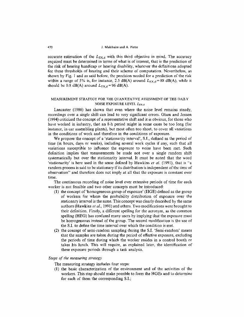
470 J. Malchaire and A. Piette
accurate estimation of the LEX,~ with this third objective in mind. The accuracy required must be determined in terms of what is of interest, that is the prediction of the risk of hearing handicap or hearing disability, whatever the definitions adopted for these thresholds of hearing and their scheme of computation. Nevertheless, as shown by Fig. 1 and as said before, the precision needed for a prediction of the risk within a range of 5% is, for instance, 2.5 dB(A) around LEX,~ = 88 dB(A), while it should be 0.8 dB(A) around LEX,d=96 dB(A).
MEASUREMENT STRATEGY FOR THE QUANTITATIVE ASSESSMENT OF THE DAILY
NOISE EXPOSURE LEVEL LBX,d
Lancaster (1986) has shown that even where the noise level remains steady, recordings over a single shift can lead to very significant errors. Olsen and Jensen (1994) criticized the concept of a representative shift and it is obvious, for those who have worked in industry, that an 8-h period might in some cases be too long (for instance, in car assembling plants), but most often too short, to cover all variations in the conditions of work and therefore in the conditions of exposure.
We propose the concept of a ‘stationarity interval’, S.I., defined as the period of time (in hours, days or weeks), including several work cycles if any, such that all variations susceptible to influence the exposure to noise have been met. Such definition implies that measurements be made not over a single random shift systematically but over the stationarity interval. It must be noted that the word ‘stationarity’ is here used in the sense defined by Hawkins et al. (1991), that is “a random process is said to be stationary if its distribution is independent of the time of observation” and therefore does not imply at all that the exposure is constant over time.
The continuous recording of noise level over extensive periods of time for each worker is not feasible and two other concepts must be introduced:
(1) the concept of ‘homogeneous group of exposure’ (HGE) defined as the group of workers for whom the probability distribution of exposure over the stationary interval is the same. This concept was clearly described by the same authors (Hawkins et al., 1991) and others. Two modifications were brought to their definition. Firstly, a different spelling for the acronym, as the common spelling (HEG) has confused many users by implying that the exposure must be homogeneous instead of the group. The second modification is the use of the S.I. to define the time interval over which the condition is met.
(2) the concept of semi-random sampling during the S.I. ‘Semi-random’ means that the samples are taken during the period of effective exposure, excluding the periods of time during which the worker resides in a control booth or takes his lunch. This will require, as explained later, the identification of these exposure periods through a task analysis.
Steps of the measuring strategy The measuring strategy includes four steps: (1) the basic characterization of the environment and of the activities of the
workers. This step should make possible to form the HGEs and to determine for each of them the corresponding S.I.;

Assessment of noise exposure and risk of hearing impairment 471
(2) the qualitative evaluation of the exposure, which concludes the first step and provides a first estimate of the L nx,d, through conventional procedures;
(3) the detailed measurements themselves; and (4) the quantitative evaluation of the results and the estimation of the LEX,d, and
of its precision. It must be emphasized that this is only one part, but a significant one, of the
hearing conservation programme, as audiometric and noise control programmes must also be developed.
The present paper will focus on steps 3 and 4 of this strategy, as step 1 has been adequately described and illustrated among others by Hawkins et al. (1991) and step 2 is amply discussed by Royster et al. (1986), along with all the conditions to be met for the calibration of the instruments and the general organizing of the measurement campaign.
PlaniJication of the measurements
At the end of steps 1 and 2, HGE groups have been formed, the corresponding S.I. defined and the periods of effective exposure during the S.I. identified.
Let us define -nHon as the number of workers belonging to a given HGE; -the series of Tie and ri, defining the times (in min) at the beginning and at the
end of the sequence i of effective exposure to noise; - To = the stationarity interval expressed in min: ( = 480 x S.I. in case of 8-h shifts); - Ti = C(rii - Tia), the total time of effective exposure to noise (in min); - T2 = TO - T1, the total time during which the worker is exposed to a noise level
L ,+a* well below [20 dB(A) at least] those met during T1 (in min). The questions to answer before performing the sampling campaign are:
On how many workers n, among the nHGE should the sampling be conducted?. One step in the interpretation will be to verify whether the group is indeed homogeneous. Therefore a sufficiently large number of workers must be chosen, to be able to observe the potential heterogeneity. Table 1 gives the number of workers n, to take into consideration in order to be sure at 95% that one of the workers from the 20% of the nHGn who would be the most exposed (Leidel et al., 1977) is included in the sample.
How many samples to take per worker ?. The same reasoning as above can be adopted: the number of sample n, per worker being chosen in order to increase the probability of encountering the noisiest conditions. Based on the approach of Leidel et al. (1977), it can be shown that five samples would be enough to be sure at 90% that one sampling period is taken during the 33% of the time with the highest noise level. This number n, = 5 could therefore be used systematically. Our experience shows that this leads to a standard error of the LEX.~ which in most cases is smaller
Table 1. Number of workers (n,) to sample as a function of the size of the homogeneous group of exposure
nHGE $6 7-8 9-11 12-14 15-18 19-26 27-43 44-50 > 50
nw nw = nHGE 6 7 8 9 10 11 12 14

472 J. Malchaire and A. Piette
than 1 dB(A). As discussed before, this is not needed in all cases and in particular for Lux,d lower than 90 dB(A). The recommended procedure is therefore to start rather arbitrarily with n,= 3 samples per workers, to go through the measuring campaign and the interpretation and to collect additional samples per person, if needed to reach the desired precision on the LEX,d.
What should be the duration of the samples?. According to our study reported in Appendix B, the accuracy of the L nx,d varies roughly as a function of the number of samples, but as a function of the square root of the sample duration At. Therefore, it appears preferable to increase n, and use short samples. The problem is not critical, however, if the Larsen (197 1) philosophy is used, assuming that the standard deviation of the noise equivalent levels (LA~J obtained from samples of duration AT2 can be estimated from the standard deviation of the L,+q values for samples of duration AT,
The mathematical expression proposed by Larsen (1971) in the field of atmospheric pollution has proved to be invalid in the field of noise and our study (Appendix B) showed that a better prediction can be obtained using the following expression:
In particular this expression will be used to derive the standard deviation for a 8-h period.
As this estimation is possible, At should be determined according to practical considerations. Samples of short duration would be possible in industries with short workcycles but would be impractical, the time spent to install the instrumentation becoming relatively too important compared to the sampling time. In the common case of workplaces with no particular cycle time, At of the order of 30-60 min appears to be most practical.
When to schedule the sampling? n,q, samples of duration At must be scheduled at random over a period of a stationarity interval and during the phases of effective exposure to noise (duration T,). This can be done using a table of random numbers.
Let ri be the ith random number. ri.TI indicates the time during the period of effective noise exposure when the sampling should start.
From the list of (T,, T,J defined previously, the time of the start of the sampling can be easily determined.
It remains to be verified whether a sample of duration AT can be taken during this sequence after the starting time and whether this scheduling is not in conflict with a previous scheduled sample. If this is the case, this random number is dropped and the computation restarted with the next one.
How to sample?. Two different measuring techniques have been used in the past: the zonal method and the ambulatory method. The zonal method was proposed as the most cost-effective method by Rockwell (1983). It consists of locating an integrating sound level meter at a point near the worker. This method provides more accurate noise measurements (no or minimum interference with the frequency

Assessment of noise exposure and risk of hearing impairment 473
response of the microphone) but the results are often not representative of the real exposure of the worker.
Dosimeters are attached to the subjects with the microphone placed near the ear. Several studies have shown that, using this procedure, the measurement errors are small (Shackleton and Piney, 1984, Erlandsson et al., 1979) and this must therefore be considered from now on as the reference method. More recently, ‘exposimeters’, that is, portable compact integrating sound level meters, have appeared on the market. They provide the possibility of recording not the total dose only, but the LAeq levels during almost any increment of time and to have a picture of the history of the exposure during the observation period. Although this capacity is not used here, it is useful to determine the characteristics of the exposure, the main noise sources and the possibilities of improving the situation.
Interpretation of the results
At the end of the measuring campaign, n,.n, values of LAeq have been recorded over periods of duration At with effective noise exposure.
The interpretation will include five steps: (1) verify the homogeneity of the HGE; (2) verify the stationarity of the results; (3) determine the normal distribution characterizing the data; (4) compute LEX,d and its standard error; and (5) interpret the result in terms of risk of handicap or disability.
Homogeneity of the HGE. Statistically, the homogeneity of the HGE can be tested using an analysis of variance with the following model:
Lij= L,+ Wj+tv
where L, is the jth LAeq measured on worker i; L, is the arithmetic mean of the n,.n, LAeq values; Wi is the effect of the worker i, that is the systematic difference from the mean L,, observed for the worker i, for the n, samples taken on that worker; and eii is the difference not explained. The analysis of variance will test whether the mean differences between workers
(WJ are significant in regard of the differences within subjects. If the differences are statistically significant, it must be concluded that the group is
not homogeneous and, by an analysis of these differences, the group can be divided in HGE subgroups. The other steps of the interpretation will then be conducted on these subgroups. It remains to allocate to these subgroups, the workers who did not participate to the sampling campaign. This must be done by going back to the workplace and to the task analysis performed in steps 1 and 2 of the measuring strategy.
Stationarity qf the results. It is obvious that a sequence of values according to time such as 92, 88, 91, 93, 87 has to be considered differently than a sequence such as 87, 88, 91, 92, 93, which would clearly indicate a trend of the noise levels during the sampling period.

414 J. Malchaire and A. Piette
In the second case, it must be concluded that the whole noise situation was not covered and the stationarity interval adopted must be questioned.
A check of the stationarity of the data can be made using the autocorrelation function (Pi-Cat, 1987; Rappaport, 1991) but this statistical tool remains difficult to understand, use and interpret. A simpler test is the linear correlation between the LAeq values and the time, during the total duration To, at which they were recorded. The correlation coefficient R is calculated and its significance tested taking into account the number of values involved.
If it is not significant, the stationarity interval can be considered to be valid and the interpretation pursued. If it is significant, it is necessary to the task analysis performed in steps 1 and 2 to look for the factors justifying the trend demonstrated by the correlation analysis and correct the S.I. The procedure of sampling must then be pursued by taking additional samples during the expanded S.I. and the interpretation phase started again.
Distribution of the observed L.+, computation of the LEX,~ and its standard error. It is common, when sampling for chemical agents, to assume that the distribution of the observed concentration is lognormal. As, in acoustics, dB values are used, it is logical-and usually assumed-that the distribution of the ~~~~ values is normal (Behar and Plener, 1984). Recordings in industry (Appendix B) prove that this is not always the case and that this assumption may lead to an underestimation-in some cases very large-of the LEX,~.
The A-weighted equivalent level over the n=n,.n, samples (with n, the number of workers sampled in a subgroup if the initial HGE was indeed split into subgroups) can be calculated according to the equal energy principle, as follows
LA~~,J- = 10 log:
The arithmetic mean of these n values is given by
m = $!?FL&.q;. ~1 j=l
If the distribution of the n values is normal, Bernard and Caste1 (1987) have shown that LA~~,J- would be given by
L,&q,T’ = m + 0.1 1 52s2
where s is the standard deviation of the n L*eqi values. The comparison of LA~~,J and LAeq,T' values gives a first indication of whether or not the distribution is indeed normal. A further indication is provided by the skewness coefficient of the distribution which is given by
where m3 is the third moment about the mean and s the standard deviation of the distribution.
Assessment of noise exposure and risk of hearing impairment 475
A positive value of g indicates a positive skewness of the distribution of the LAeqi values.
If the distribution is not normal, we propose to compute, from the Bernard and Caste1 expression, the standard deviation of the normal distribution with the mean equal to m and the overall equivalent level LAeq,T by
s = ~LA.w,T _ m
0.1152 .
This procedure will be discussed in Appendix B reporting the field study. The daily noise exposure level can then be estimated by
LEX,d = 10 log [ & (Ti 10LA~J”o + T*lOLA@“O 1 .
As, in the majority of the cases, the level LAeqZ is more than 20 dB lower than LAeq,=, the above formula can be simplified to
.t&,d = LA~~,T + 10 logT’. To
The standard deviation derived above concerns the distribution of samples of duration At. As stated earlier, it is possible to derive the standard deviation for a sampling period of 8 h from
At 0.31
G? = s 480 ( >
- .
Finally, the standard error of the L nx,d can be estimated from the following formula (Bernard and Caste& 1987)
where n is the number of samples for the HGE group or subgroup. The 95% confidence interval can then be estimated as
[LEX,d - te, LEX,d + te]
where t is the value of the variable t of student for a bilateral risk of error of 5% and (n- 1) degrees of freedom.
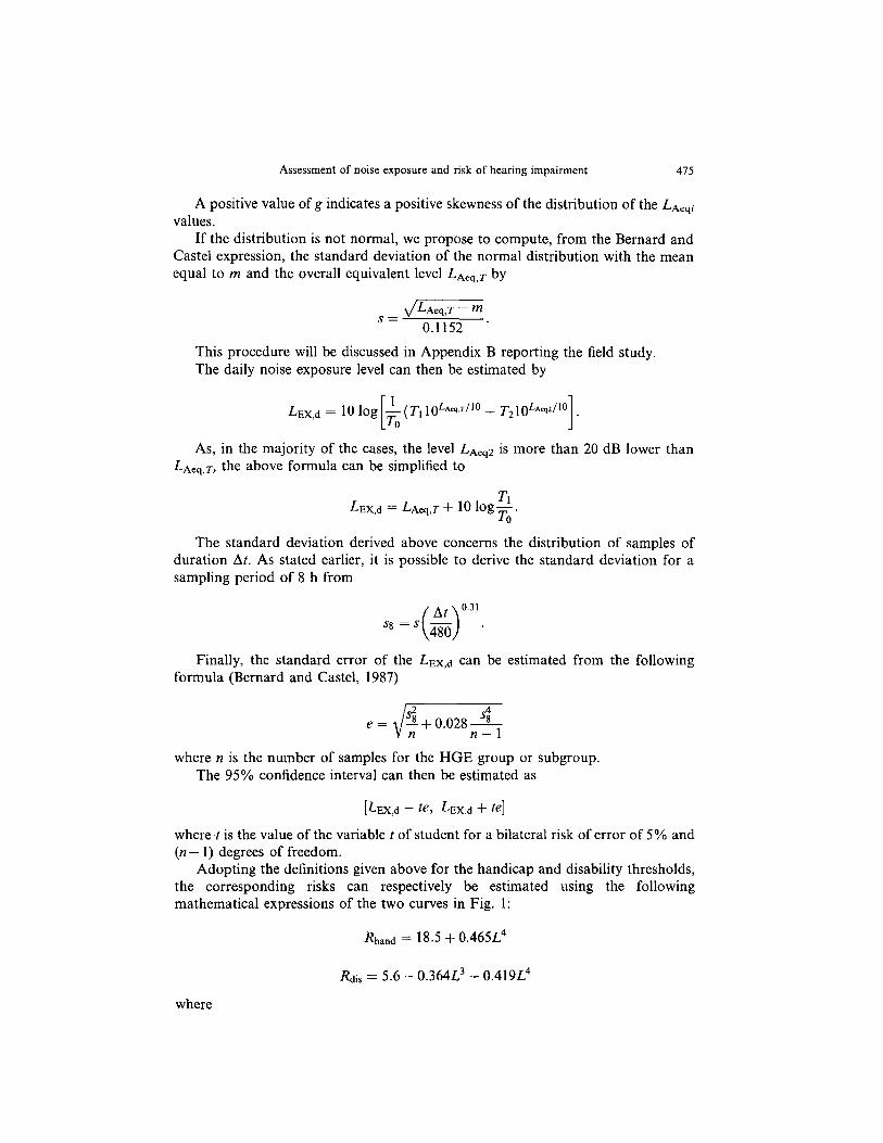
Adopting the definitions given above for the handicap and disability thresholds, the corresponding risks can respectively be estimated using the following mathematical expressions of the two curves in Fig. 1:
R hand = 18.5 + 0.465L4
Rdis = 5.6 - 0.364L3 + 0.419L4
where

476 J. Malchaire and A. Piette
L = LEX,d - 70 10 .
It is also possible to determine from Fig. 1 whether the accuracy (&le) of the Lnx,d is sufficient for a given precision of, for example, f2.5% on the risk. If it is not the case, the sampling campaign must be pursued by collecting additional samples of the same duration At on each selected worker.
DISCUSSION
The approach described in this paper aims at the determination of the Lux,d values for epidemiological purposes and for the predicting the hearing ‘risk’ encountered by an individual worker in the context of a hearing conservation programme. This is in opposition with the ‘compliance’ approach aiming simply to determine whether exposure exceeds the limits defined by the law.
An innovating point of the approach is to clearly define the ‘risk’ as the probability for an individual to develop hearing impairment above a given threshold during his professional life. The definitions of the maximum hearing deficits (in terms of audiometric frequencies and levels) are outside the scope of this paper but those presented as an illustration are used in some countries among which is Belgium. Whatever the definition used, it remains that the precision needed on the daily noise exposure level for a given precision on the risk is dependent on that level and can be rather weak for LEX,~ levels around 90 dB(A). This is in opposition to proposals by Royster et al. (1986), who recommend simply to classify the Lex,d levels in 5 dB(A) categories, as well as by Atzeri (1992), who described a statistical method to reach a precision of f 1 dB(A).
A comprehensive sampling strategy and interpretation procedure is proposed to determine the daily noise exposure level of a group of workers. The main points of this strategy are:
-the use of the concept of ‘homogeneous group of exposure’ (HGE) previously used almost exclusively for the evaluation of the exposure to chemical agents;
-the definition of a new concept, the stationarity interval, as the period over which the distribution of exposure is the same for the members of the HGE. This interval, although implicit in the definition of the HGE given by Hawkins et al. (1991), appeared to be lacking in the sampling procedure described by these authors.
-the use of an analysis of variance to test whether the group is homogenous or not, and of a regression analysis to test the validity of the stationarity interval;
-a procedure to derive the standard deviation of a normal distribution equivalent to the actual distribution, and to extrapolate from a sampling duration AT, to any duration AT2 and in particular to an 8-h period.
It must be noted that the two tests for the homogeneity of the group and the validity of the stationarity interval make the assumption that the results are normally distributed. This appears difficult to avoid as more sophisticated analyses would be too complicated. Furthermore, skewness in the distribution of the data tends to produce more significant results in the F-tests and therefore would lead to split more often then needed the HGE into subgroups (Snedecor and Cochran,

Assessment of noise exposure and risk of hearing impairment 477
1968). This appears preferable to keeping in the same group, subjects who actually have not the same exposure distribution.
The correction of the standard deviation to fit a normal distribution for the computation of the standard error appears a rather simple way to take into account, in particular, the positive skewness of the distribution of LAeq levels. Indeed, due to the equal energy principle, the accuracy of the daily noise exposure is conditioned mainly by the distribution of the highest levels. The adjustment of the normal distribution on that part of the actual distribution appears therefore justified. This adjustment is based on the work by Bernard and Caste1 (1987) and discussed by Armstrong (1992). Nevertheless, the user must be cautious to verify the shape of the distribution of the recorded values and check the validity of any data that would clearly deviate from the normal distribution. This can usually be done easily by checking the linearity of the normal probability plot of the cumulated distribution.
The strategy and interpretation described in the present paper are based on the work by Brunn et al. (1986) and Hawkins et al. (1991) for the first steps of collection of the basic information and forming of the homogeneous groups of exposure. It uses a semi-random sampling by excluding the periods without significant exposure to noise (less by about 20 dB(A) than the average noise level during real work) from the sampling period. This was adopted from the study by Damongeot and Kusy (1990) who showed that a totally random sampling would lead to significant errors on the LEX,d levels. ThiCry et al. (1994) described the ergonomic study on the basis of which this exclusion can be performed.
The proposed strategy seems not to consider the case of impact noise. The European directive (1986), translated in national law in each country of the European Union, requires different actions for the workers exposed to one or more peak levels above 140 dB. The occurrence of such impact noises can be detected easily during the ergonomic study preceding the sampling campaign and the determination of whether or not a worker is exposed to recurrent impact noise should not be a major problem. This type of exposure will lead to a distribution of LAeq levels from the n,.n, samples with a positive skewness, some of them being influenced by the occurrence of one or more impacts. As an example, a single type B (Coles and Rice, 1967) impact noise of 140 dB peak with a duration of 50 ms can roughly be assimilated at a constant noise of 94 dB(A) for 30 min. Therefore, if the LAeq level without the impact is 90 dB(A), the L*eq level with it will be 95.5 dB(A).
The interpretation procedure takes this into account in two ways, by computing the overall LAeq,T level using the exponential averaging and by adjusting the standard deviation-in this case increasing it-to improve the fitting of a normal distribution at these high levels.
REFERENCES
Armstrong, B. G. (1992) Confidence intervals for arithmetic means of lognormally distributed exposures. American Industrial Hygiene Association Journal 53, 481-485.
Attfield, M. D. and Hewett, P. (1992) Exact expressions for the bias and variance of estimators of the mean of a lognormal distribution. American Industrial Hygiene Association Journal 53, 432-435.
Atzeri, S. (1992) Impostazione metodologica della misura dell’esposizione personale al rumore (A methodological approach to personal noise exposure). Md Lav. 83, 278-288.

478 J. Malchaire and A. Piette
Behar, A. and Plener, R. (1984) Noise exposure-sampling strategy and risk assessment. American Industrial Hygiene Association Journal 45, 105-109.
Bernard, M. and Caste], J. C. (1987) Nouvelle methode d’tvaluation du bruit au travail (A new method for the evaluation of occupational noise exposure). Pre’ventique 13, 51-54.
Brunn, I. O., Campbell, J. S. and Hutzel, R. T. L. (1986) Evaluation of occupational exposure: a proposed sampling method. American Industrial Hygiene Association Journal 47, 229-235.
Burdorf, A. (1993) Bias in risk estimates from variability of exposure to postural load on the back in occupational groups. Scandinavian Journal of Work Environmental He&h 19, 50-54.
Burdorf, A. (1995) Reducing random measurement error in assessing postural load on the back in epidemiologic surveys. Scandinavian Journal of Work Environmental Health 21, 15-23.
Coles, R. R. A. and Rice, C. G. (1967) Hazards from impulse noise. Annals ofOccupationo[ Hygiene 10, 381-388.
Damongeot, A. and Kusy, A. (1990) Pertinence de l’echantillonnage ‘en aveugle’ pour l’estimation des niveaux sonores en entreprises (Relevancy of random sampling for the estimation of noise levels in industry). Cahiers de notes documentaires, INRS, ND 1778-l 39-90, 347-361.
European Communities (1986) Council directive of May 12, 1986 on the protection of workers from the risks related to exposure to noise at work, Official Journal of European Communities, L137, 28-34.
Erlandsson, B., Hakansson, H., Iversson, A. and Nilsson, P. (1979) Comparison between stationary and personal noise dose measuring systems. Acta Otolaryngologica Suppl. 360, 105-108.
Hawkins, N. C., Norwood, S. K. and Rock, J. C. (1991) A strategy for occupational exposure assessment. American Industrial Hygiene Association, Akron, Ohio, U.S.A.
IS0 1999 (1990) Determination of the occupational noise exposure and estimation of the noise induced hearing impairment. International Standard Organisation, Geneva.
Lancaster, G. K. (1986) Personal noise exposure. Part 2. a summary of a six-month survey at three collieries. Colliery Guardian, May, 213-216.
Larsen, R. I. (1971) A mathematical model for relating air quality measurements to air quality standard. Environmental Protection Agency, Office of Air Programs. Research Triangle Park, North Carolina, U.S.A.
Leidel, N. A., Busch, K. A., Lynch, J. R. (1977) Occupational exposure sampling strategy manual. National Institute for Occupational Safety and Health, Cincinnati, U.S.A.
Olsen, E. and Jensen, B. (1994) On the concept of the “normal” day: quality control of occupational hygiene measurements. Applied Occupational Environmental Hygiene 9, 245-255.
P&at, B. (1987) Application of geostatistical methods for estimation of the dispersion variance of occupational exposures. American Industrial Hygiene Associution Journal 48, 877-884.
Rappaport, S. M. (1991) Assessment of long-term exposures to toxic substances in air. Annals of Occupational Hygiene 35, 61-121.
Rappaport, S. M. and Selvin, S. (1987) A method for evaluating the mean exposure from a lognormal distribution. American Industrial Hygiene Association Journal 48, 374379.
Rappaport, S. M., Kromhout, H. and Symanski, E. (1993) Variation of exposure between workers in homogeneous exposure groups. Americun Industriul Hygiene Associution Journul54, 654662.
Rockwell, T. H. (1983) Personal vs. area noise exposure monitoring. Nationul Safety News, September, 9&93.
Royster, L. H., Berger E. H. and Royster J. D. (1986) Noise surveys and data analysis. In Noise und Hewing Conservation Manual, eds E. H. Berger, W. D. Ward, J. C. Morrill and L. H. Royster. American Industrial Hygiene Association, Fairfax, Virginia, U.S.A.
Shackleton. S. and Pinev. M. D. (1984) A comparison of two methods of measuring personal noise exposure. Annals of &cupational Hygiene 28,-373390.
- _
Snedecor, G. W. and Cochran, W. G. (1968) Statistical Metho&. The IOWA State University Press, Ames, Iowa, U.S.A.
Thiiry, L., Louit, P., Lovat, G., Lucarelli, D., Raymond, F., Servant, J. P., Signorelli, C. (1994) Exposition des travailleurs au bruit-Methode de mesurage (Occupational exposure to noise- measuring method). I.N.R.S., France.
APPENDIX A: EXAMPLE
The strategy will be illustrated in the case of a group of welders in a mechanical industry working from 7 a.m. to 3 p.m. From the task and environment analyses, it has been decided that two HGE can be formed with respectively six and nine

Assessment of noise exposure and risk of hearing impairment 479
workers. The procedure will be illustrated for the second group for which the S.I. is estimated at 10 days. We have therefore successively used:
-nnGE = 9 workers; -S.I = 10 days: monitoring period; -total duration of the monitoring period: r0 = 80 h = 4800 min; -number of workers to be sampled: n, = 7; -number of samples per worker: n, = 3 to begin; -duration of the samples: At = 30 min; -duration of effective exposure to noise: Ti = 65 h = 3900 min as the workers
spend 30 min for lunch and 1 h per day restocking the workplace from the warehouse and fulfilling some administrative work;
-duration of the periods with non-effective exposure to noise T2= 15 h=900 min;
-noise level during these periods: below 70 dB(A). Twenty-one measurements (n,q,) are performed according to a schedule easily
defined and the procedure will not be illustrated here. Table 2 provides the results. The results of the analysis of variance concerning the homogeneity of the HGE
are given in Table 3. The mean values per subject range from 89.3 to 93 dB(A) but these differences
are not statistically significant. Therefore, the group can be considered as being homogeneous.
The correlation coefficient between the L*eq values and times of measurement is R= -0.23 and is not statistically significant, indicating that there is no systematic trend of the ~~~~ values during the measuring campaign and therefore that the stationarity interval is valid.
Table 2. Schedule of the sampling and corresponding A-weighted equivalent levels LAcq,
Sample Day Hour
1 1 1.24 a.m. 2 1 8.31 a.m. 3 1 1.17 p.m. 4 2 7.10 a.m. 5 2 9.14 a.m. 6 2 12.27 a.m. I 2 2.06 p.m. 8 3 8.15 a.m. 9 4 7.40 a.m.
10 4 8.58 a.m. 11 4 2.29 p.m. 12 5 1.24 a.m. 13 6 9.12 a.m. 14 6 12.38 p.m. 15 6 1.30 p.m. 16 7 1.50 p.m. 17 9 11.13 a.m. 18 9 1.58 p.m. 19 10 10.12 a.m. 20 10 11.22 a.m. 21 IO ‘I.30 p.m.
Cumulated time (min)
24 91
377 490 614 177 906
1055 1540 1618 1889 2004 2532 2738 2190 3290 4093 4258 4512 4582 4710
Subject Replication LAeq dJ%‘V
1 1 95 2 1 92 4 1 92 5 1 89 1 2 90 6 I 96 2 2 86 7 1 95 5 2 95 2 3 90 6 2 88 3 1 95 6 3 87 4 2 94 3 2 93 7 2 89 I 3 94 3 3 89 7 3 93 4 3 88 5 3 88

480 J. Malchaire and A. Piette
Table 3. Analysis of variance of the L *eai 1 evels for the differences between workers
Source of variation Sum of square Degrees
of freedom Mean square F test Probability
Between subjects 30.7 6 5.1 0.43 0.85 Within subjects 166.0 14 11.9 Total 196.7 20
The overall L*eq,T level computed according to the equal energy principle for the 21 values is equal to 92.3 dB(A), while the arithmetic mean and standard deviation are 9 1.3 and 3.1 dB(A). The corrected standard deviation computed from the LAeq,T and mean values according to the Bernard and Caste1 (1987) expression is equal to 3.0 dB(A), the distribution presenting a slight negative skewness (skewness coefficient: - 0.072).
The daily exposure level is then:
,t,EX,d = 92.3 + 10 log; = 91.4 dB(A)
From the standard deviation s= 3.0 dB(A) for 30 min samples, the standard deviation for 8-h samples dan be derived:
sg = 3.0 -gj ( >
0.31
= 1.3
and the standard error can be estimated equal to:
e = 0.3 dB(A).
For 21 values, the t value at the 95% level of confidence is equal to 2.086 and therefore the 95% confidence interval of L nx,d is 91.4f0.6 dB(A). This precision is largely sufficient and no further measurements are needed.
The risks of hearing handicap and disability are respectively estimated at 28% and 11% at age 60 years after 40 years of exposure to that LEX,~.
APPENDIX B: BACKGROUND STUDY
Introduction
The strategy described in the paper uses concepts and formulas presented and validated in the literature. However, it appeared necessary to verify whether some hypotheses, and in particular the Larsen (1971) model, defined in the field of environmental pollution, are also valid in the context of noise exposure assessment. A database was built in order to test these hypotheses.
Material and methods
Twenty-two workers performing different tasks in different companies were surveyed for 8 h per day during 10 consecutive days of work. These included mechanics, bricklayers and operators for different machines from several sectors of a steel industry and from a manufacture of metallic parts. All were characterized by

Assessment of noise exposure and risk of hearing impairment 481
601 I / I I I I I
0 1 2 3 Tim: 5 6 7 (h)
Fig. 2. Example of an 8-h recording of the 1 min equivalent levels.
fluctuating conditions of noise as typically illustrated in Fig. 2, with some periods spent in less noisy areas (such as control rooms or cafeteria).
A Larson Davis LD705 exposimeter was used, recording the equivalent level every minute. From a task analysis, phases with non-effective exposure to noise were excluded u priori, leaving a database of a total of 68 713 min of recording.
For each worker, sampling strategies were simulated, as explained above, with -the number of samples n, varying from 3 to 20; -the duration of sampling At varying from 5 to 180 min. The n, samples were taken at random during the period of effective exposure to
noise (duration rr) for each worker. The procedure was repeated 5000 times in each case and for each subject and a
list of 5000 L,4eq,T was obtained. The variance of these 5000 values (8:) was computed. Figure 3 illustrates, for two of the 22 workers, how this variance varies as a function of n, and At.
For the whole group of subjects, a covariance analysis was performed with log(s*) as dependent variable, the number of the subject as independent variable and log(n,) and log(At) as covariates.
Rtkdts
This analysis of covariance provided the following expression
s; = wi 1 ,0.95&0.62 s
where Wi is a factor depending on the worker and his working condition.

482 J. Malchaire and A. Piette
14
i3nS
I i 12-‘\5 : I
I \,7 I I
\ I I
,o- i,lO i I
3 : l2 ’ \Is :
E a- a
‘,17 \
.L( ‘20 \ \
iL3- ‘\
b- \ \
5
4-
k
7 10
l2 2- 1517
20
O----x-- 5 15 20 30
I I
I I
\
L ‘\.
so
I I i I I \ I \ \ ‘1
\
L
I ‘\ \ \
\ \ -2
so 120 180
AT (min) Fig. 3. Variance of the distribution of L *cq levels as a function of the number of samples n, and the
sampling duration At.
The overall multiple correlation coefficient was 0.974 and both exponents were significant at P < 0.001.
This indicates, as used in the strategy, that the accuracy varies roughly inversely proportionally to the number of samples and the square root of the sample duration. From this expression, it follows that:
and therefore
This formula is proposed instead of the one presented by Larsen (197 1) to derive the standard deviation for a sampling duration At* from the standard deviation for another sampling duration.
SAT hereabove is the standard deviation of the LAeq,= values obtained through the 5000 simulations on the database of each subject. In practice, only one campaign of n,.n, samples of duration At will of course be conducted. Therefore the only estimate of $A, is the standard deviation of the n,.n, LAeq values.
A second procedure proposed in the interpretation of the data needed validation: the computation of the standard deviation from the energetic and arithmetic means
(LA~~,T and m) of the distribution of LAaqi values.

Assessment of noise exposure and risk of hearing impairment 483
Table 4. A-weighted equivalent level (LA&; mean (m) and standard deviation (s) of the 1 min levels; equivalent level (L’A~~ derived from m and s;
corrected standard deviation (s,,) and skewness coefficient (sk) for the noise recordings on 22 subjects in various exposure conditions
n LAqT m s cAeq,T &or Sk
1 89.0 85.7 5.8 89.6 5.4 -0.78 11 89.6 87.0 5.1 89.9 4.8 -0.60 10 88.9 85.9 5.6 89.5 5.2 -0.57
3 88.9 86.2 4.9 89.0 4.8 -0.54 4 88.8 85.8 5.3 89.1 5.0 -0.41
ll? 88.4 86.8 3.8 88.5 3.7 -0.38 19 91.4 89.4 4.3 91.6 4.1 -0.29 22 91.7 89.2 4.6 91.7 4.7 -0.29
6 87.7 84.1 5.6 87.7 5.6 -0.04 16 89.0 87.6 3.4 88.9 3.4 0.00 13 91.2 88.0 5.2 91.1 5.2 0.06
5 87.6 83.0 5.8 86.8 6.3 0.07 2 88.1 85.1 4.9 87.8 5.2 0.09
15 88.6 85.8 4.7 88.4 4.9 0.12 8 88.7 84.1 6.2 88.6 6.3 0.18 9 88.1 83.3 6.1 87.7 6.5 0.28
14 90.5 85.8 6.1 90.0 6.3 0.30 7 87.2 82.4 5.4 85.7 6.5 0.51
20 92.3 89.4 4.5 91.7 5.0 0.56 12 89.7 87.3 4.0 89.2 4.5 0.56 17 89.3 86.2 4.1 88.2 5.2 0.72 21 93.4 88.9 4.3 91.0 6.3 1.36
16
14-
13-
12-
Lhgende
- 1 : hist ---_ 2:s .._... 3:-
Lti in dB(A)
Fig. 4. Histogram (l), fitted normal distribution (2) and adjusted normal distribution (3) in the case of a distribution of L*cq level with negative skewness (worker no. 1).
484 J. Malchaire and A. Piette
15
14-
13-
12.
LBgende
- 1 : hist ---. 2:s . .._... 3:scor
11 -
@ lo- .I 4 a I a-
2 7-
$ “,- 2 4-
3-
2-
l- ,' ,' ___.---
0-p / I I 60 70 60 90 100 110 12 0
Lh in dB(A)
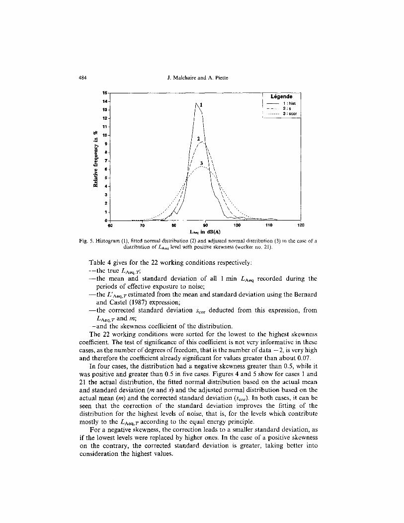
Fig. 5. Histogram (I), fitted normal distribution (2) and adjusted normal distribution (3) in the case of a distribution of L,&q level with positive skewness (worker no. 21).
Table 4 gives for the 22 working conditions respectively: -the true LA~~,~; -the mean and standard deviation of all 1 min LAeq recorded during the
periods of effective exposure to noise; -the L’A~~,~ estimated from the mean and standard deviation using the Bernard
and Caste1 (1987) expression; -the corrected standard deviation s,,, deducted from this expression, from
L Aeq,T and m
-and the skewness coefficient of the distribution. The 22 working conditions were sorted for the lowest to the highest skewness
coefficient. The test of significance of this coefficient is not very informative in these cases, as the number of degrees of freedom, that is the number of data - 2, is very high and therefore the coefficient already significant for values greater than about 0.07.
In four cases, the distribution had a negative skewness greater than 0.5, while it was positive and greater than 0.5 in five cases. Figures 4 and 5 show for cases 1 and 21 the actual distribution, the fitted normal distribution based on the actual mean and standard deviation (m and S) and the adjusted normal distribution based on the actual mean (m) and the corrected standard deviation (scar). In both cases, it can be seen that the correction of the standard deviation improves the fitting of the distribution for the highest levels of noise, that is, for the levels which contribute mostly to the LA~~,J- according to the equal energy principle.
For a negative skewness, the correction leads to a smaller standard deviation, as if the lowest levels were replaced by higher ones. In the case of a positive skewness on the contrary, the corrected standard deviation is greater, taking better into consideration the highest values.