
A Complex Adaptive System Approach to QoS Assurance and Stateful Resource Management for Dependable...
51
A Complex Adaptive System Approach to QoS Assurance and Stateful Resource Management for Dependable Information Infrastructure (CIP Project) Nong Ye (PI) Professor of Industrial Engineering, Affiliated Professor of Computer Science and Engineering Ying-Cheng Lai (co-PI) Professor of Electrical Engineering and Mathematics Partha Dasgupta (co-PI) Associate Professor of Computer Science and Engineering Collaborators: AFRL (John Faust and Pat Hurley) October 18, 2002
-
date post
20-Dec-2015 -
Category
Documents
-
view
218 -
download
2
Transcript of A Complex Adaptive System Approach to QoS Assurance and Stateful Resource Management for Dependable...

A Complex Adaptive System Approach toQoS Assurance and Stateful Resource Management for
Dependable Information Infrastructure(CIP Project)
Nong Ye (PI)
Professor of Industrial Engineering, Affiliated Professor of Computer Science and Engineering
Ying-Cheng Lai (co-PI)
Professor of Electrical Engineering and Mathematics
Partha Dasgupta (co-PI)
Associate Professor of Computer Science and Engineering
Collaborators: AFRL (John Faust and Pat Hurley)
October 18, 2002

Presentation Outline
Project overview Year 1 work
QoS requirements – Nong Ye local-level QoS models (router and web server) – Nong Ye Simulation model of Internet – Nong Ye Mathematical theories on networks and attacks – Ying-Cheng Lai Trust and security models of networks – Partha Dasgupta
Year 2 work and plan Regional-level QoS models – Nong Ye Detection of emergent network states – Nong Ye Mathematical theory on phase transition in networks – Ying-Cheng Lai Trust and security model of networks – Partha Dasgupta

Project Overview
Goal Develop the bottom-up self-synchronization of QoS-centric stateful
resource management, according to a Complex Adaptive Systems approach, for a dependable information infrastructure that will be used to host network-centric information operations
Objectives Investigate, implement and test two enabling elements of the dependable
information infrastructure: Control strategies to enable the bottom-up self-synchronization of QoS-centric
stateful resource management Control and communication protocols to embed the control strategies of self-
synchronization into the existing information infrastructure for making it dependable at affordable costs
Year 1 research: local-level QoS and security Year 2-3 research: regional-level QoS and security Year 4-5 research: global-level QoS and security

QoS Requirements
Without QoS requirements, any QoS level is acceptable Sensitivity of various traffic data on computer networks
QoS Attributes Timeliness Precision Accuracy
QoS Requirements
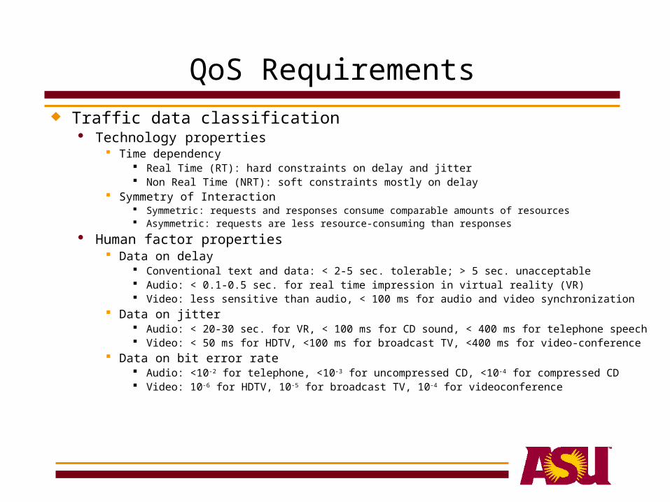
Traffic data classification Technology properties
Time dependency Real Time (RT): hard constraints on delay and jitter Non Real Time (NRT): soft constraints mostly on delay
Symmetry of Interaction Symmetric: requests and responses consume comparable amounts of resources Asymmetric: requests are less resource-consuming than responses
Human factor properties Data on delay
Conventional text and data: < 2-5 sec. tolerable; > 5 sec. unacceptable Audio: < 0.1-0.5 sec. for real time impression in virtual reality (VR) Video: less sensitive than audio, < 100 ms for audio and video synchronization
Data on jitter Audio: < 20-30 sec. for VR, < 100 ms for CD sound, < 400 ms for telephone speech Video: < 50 ms for HDTV, <100 ms for broadcast TV, <400 ms for video-conference
Data on bit error rate Audio: <10-2 for telephone, <10-3 for uncompressed CD, <10-4 for compressed CD Video: 10-6 for HDTV, 10-5 for broadcast TV, 10-4 for videoconference

QoS Requirements
Traffic data classification
QoS Requirements
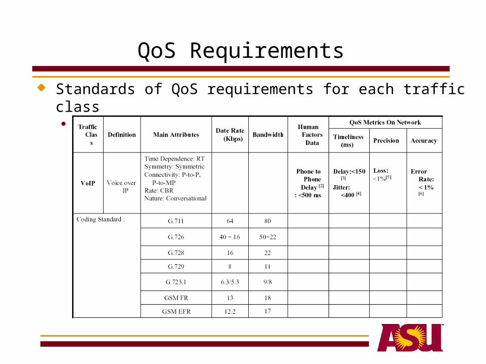
Standards of QoS requirements for each traffic class Voice over IP
QoS Requirements
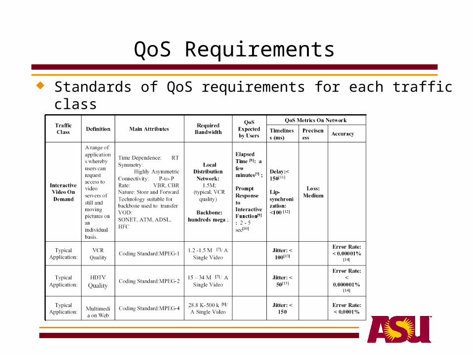
Standards of QoS requirements for each traffic class Video on demand

Local-Level QoS Models
Existing models Best effort (BE): current Internet, FIFO, no resource reservation, no
service service differentiation, no service guarantee Differential service (DS): DiffServ, RFC2475, per-hop service control,
coarse granularity of service differentiation through traffic classification, conditioning, priority queuing, bandwidth allocation by service class, weak service guarantee, stateless
Integrated service (IS): InteServ, RFC1633, end-to-end bandwidth reservation through RSVP, queuing to enforce bandwidth allocation, firm end-to-end per-flow service guarantee, problems in scalability and flexibility
Goals Minimize execution time Maximize resource utilization Maximize throughput

Local-Level QoS Models
QoS principles Resource agents cannot provide end-to-end service guarantee to user agents Process agents need to be proactive in seeking right resource agents to meet
their end-to-end QoS requirements QoS goal of local-level resource agents
Performance stability and thus predictability through bounded or least variable performance
Service differentiation Guaranteed if admitted
Local-Level QoS Models
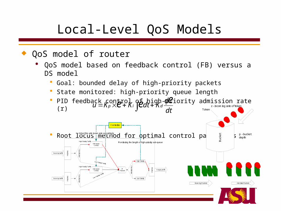
QoS model of router QoS model based on feedback control (FB) versus a DS model
Goal: bounded delay of high-priority packets State monitored: high-priority queue length PID feedback control of high-priority admission rate (r)
Root locus method for optimal control parameters
dt
dKdtKKueee dip
Controller
Monitoring the length of high-priority sub-queue
Adjust the admission rate accordingly
Classification
Classification
InterfaceInterface
AdmissionControl
High Priority Traffic
AdmissionControl
High Priority Traffic
Low Priority Traffic
IPForward
Low Priority Traffic
High Priority
Low Priority
Incoming traffic
Incoming traffic
Outging traffic
Classification
Interface
Buc
ket
Incoming Packets
Tokenr - incoming rate of token
p - bucketdepth
Admitted Packets
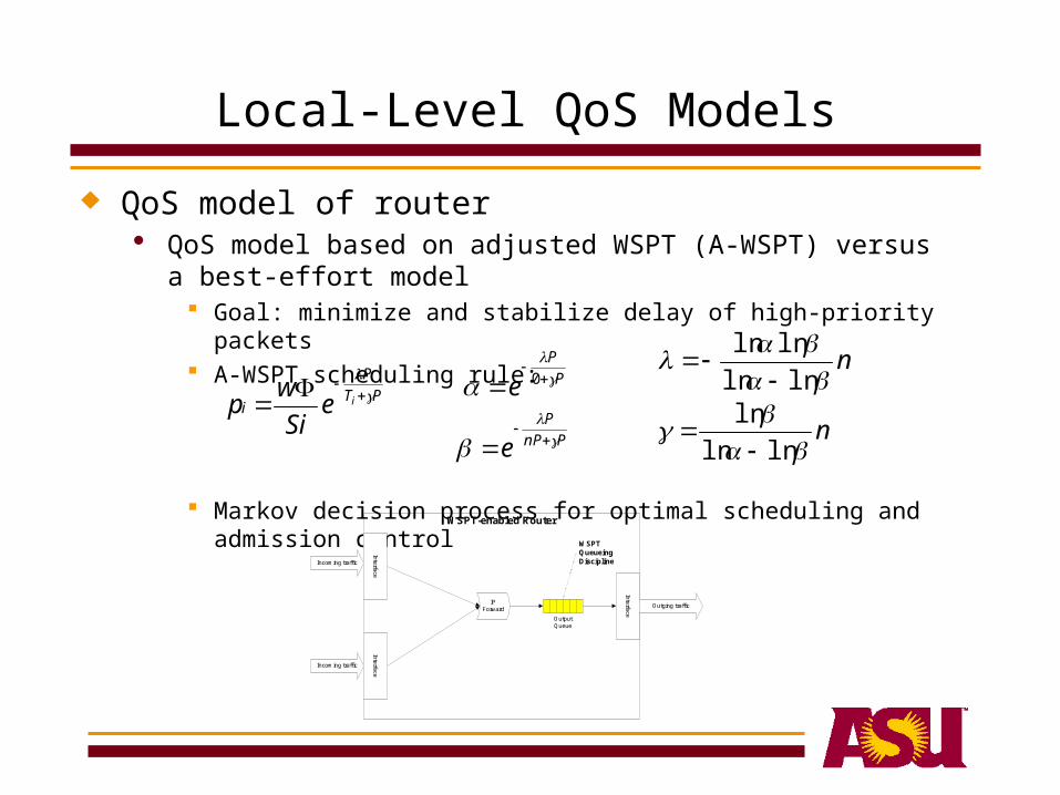
Local-Level QoS Models
QoS model of router QoS model based on adjusted WSPT (A-WSPT) versus a best-
effort model Goal: minimize and stabilize delay of high-priority packets A-WSPT scheduling rule:
Markov decision process for optimal scheduling and admission control
PT
P
i ieSi
wp
WSPT-enabled Router
IPForward
Inte
rface
Incoming traffic
Incoming traffic
Outging traffic
OutputQueue
WSPTQueueingDiscipline
Inte
rface
Inte
rface
P
P
e
0
PnP
P
e
n
lnln
lnln
n
lnln
ln
Local-Level QoS Models
QoS models of router OPNET simulation experiments
Parameters of router models BE: FIFO queuing, no admission control WSPT and A-WSPT: WSPT and A-WSPT queuing, no admission control, W=5 for
high-priority packets, W=2 for low-priority packets DS: token rate=400,000 bits/sec, bucket depth=100,000 bits, high-priority
queue=100,000 bits, low-priority queue=450,000 bits FB: Kp = 1.0, Ki = 0.2, Ki = 0.2, Control bound value = 80,000 bits, other
configurations are same as those for DS Experiment set-up
Each source generates either high-priority packets or low-priority packets, NOT both• Inter-arrival time: exponential distribution• Packet size: normal distribution, mean=10,000 bits, standard deviation=2,000
bits One output interface: Service rate 640,000 bits/sec Total output queue space: 550,000 bits Two types of packet: High priority: ToS value=7, Low priority: ToS value=0 Simulation duration: 180 seconds

Local-Level QoS Models
QoS models of router OPNET simulation experiments
Experimental set-up Interface Start time End time Rate(Sec) (Sec) Distribution Mean (Sec) (bits/sec)
1 Src0 0 0 180 Exponential 0.04000 250,0002 Src1 0 0 180 Exponential 0.10000 100,0003 Src2 0 0 180 Exponential 0.06667 150,0004 Src3 1 0 180 Exponential 0.04000 250,0005 Src4 1 0 180 Exponential 0.10000 100,0006 Src5 1 0 180 Exponential 0.06667 150,000
Traffic source Interarrival timeHeavy Traffic
Interface Start time End time Rate(Sec) (Sec) Distribution Mean (Sec) (bits/sec)
1 Src0 0 0 180 Exponential 0.13333 75,0002 Src1 0 0 180 Exponential 0.13333 75,0003 Src2 0 0 180 Exponential 0.06667 150,0004 Src3 1 0 180 Exponential 0.13333 75,0005 Src4 1 0 180 Exponential 0.13333 75,0006 Src5 1 0 180 Exponential 0.06667 150,000
Light TrafficTraffic source Interarrival time
Interface Start time End time Rate(Sec) (Sec) Distribution Mean (Sec) (bits/sec)
1 Src0 0 60 120 Exponential 0.05000 200,0002 Src1 0 0 180 Exponential 0.06667 150,0003 Src2 0 0 180 Exponential 0.06667 150,0004 Src3 1 60 120 Exponential 0.05000 200,0005 Src4 1 0 180 Exponential 0.06667 150,0006 Src5 1 0 180 Exponential 0.06667 150,000
Traffic source Interarrival timeHybrid Traffic

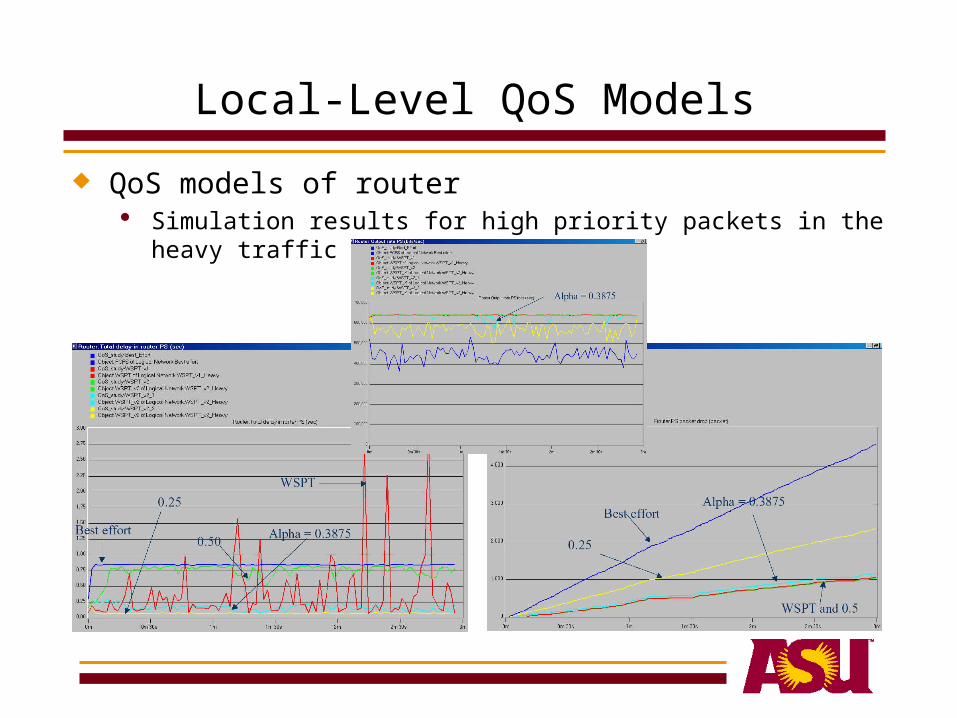
Local-Level QoS Models
QoS models of router Simulation results for high priority packets in the heavy traffic condition
Local-Level QoS Models
QoS models of router Simulation results for high priority packets in the heavy traffic condition

Local-Level QoS Models
QoS models of router Overall simulation results
For the heavy traffic condition Feedback control
o Shortest time-in-system for high-priority packets with low variationo Lowest packet loss for high-priority packetso High throughput for high-priority packets
DiffServo Generally similar performance to FBo Higher loss of high-priority packets at the output queueo Slightly better throughput of high-priority
WSPTo Highest throughput for high-priority traffic.o Variable time-in-system, because WSPT allows newly arriving packets to push back lower-priority packets
A-WSPTo Comparable to WSPT but with more stable time-in-system
Best efforto Similar performance for high and low priority packets
For the light traffic conditiono Packet loss: no packet loss for all modelso Time-in-system of high-priority traffic: WSPT is best but similar to DS and FB, BE is much worse

Local-Level QoS Models
QoS models of web server Web requests with due time Admission control: if completion time > due time, reject
QoS models based on production planning for single machine, parallel machines (cluster of web servers) and serial-machines (multiple steps)
WSPT: schedule by Wj/Pj
ATC: combine WSPT with minimum slack time, EDD: schedule by the earliest due date
pk
tpd
p
wtI jj
j
jj
0,maxexp)(
1
2
n
clients
WSPT Queue server
Admission Control
Admission Control

Local-Level QoS Models
QoS models of web server OPNET simulation experiments
Five models: BE, DS, WSPT, ATC, EDD Three scenarios
Heavy traffic• Traffic Generation
Weight: 1,2,3,6Packet inter-arrival time distribution: exponential (0.04) for W1,
W2, W3, and exponential (0.2) for W6
Packet size distribution: Normal(6000,1000) bitsTraffic generated: 480,000 bits per second in averageDue date distribution: Normal(0.8,0.08)
• QueueService Rate: 240,000 bits per secondCapacity: 512,000 bits. For DS, capacity of high-priority queue
is 32,000; capacity of low-priority queue is 480,000
• K value for ATC = 1000 Longer due time
• Traffic Generation: due date distribution of Normal(2,0.2) Less queue capacity
• Queue capacity: 128,000 bits. For DS, capacity of high-priority queue is 8000; capacity of low-priority queue is 120,000

Local-Level QoS Models
QoS models of web server Simulation results for the heavy traffic condition
Local-Level QoS Models
QoS models of web server Overall simulation results
Effects of due time and admission control: less drop at the queue Effects of longer due time: longer queue length Effects of less queue capacity
Smaller lateness of all traffic for all five models, W6, W3 and W1, because of a smaller queue
DS drops more W6 Production planning & admission control keeps the lateness of all
requests < 0 For W6 requests: WSPT/ATC is similar to DS in producing the
best performance For W3 and W1 requests: WSPT/ATC is better than DS

Simulation Model of Internet
Goals Build a simulation model of Internet using scale-free model of
Internet Discover data collection points, metrics and analytical techniques to
detect emergent network states
Research stages

Simulation Model of Internet
Research stages Stage 1
Write program which implements the scale-free algorithm to build up internet topology:
max # of nodes: n = 5,000# of connections: m = 1Initial # of nodes = n0 = m
Stage 2 Classify devices as follows
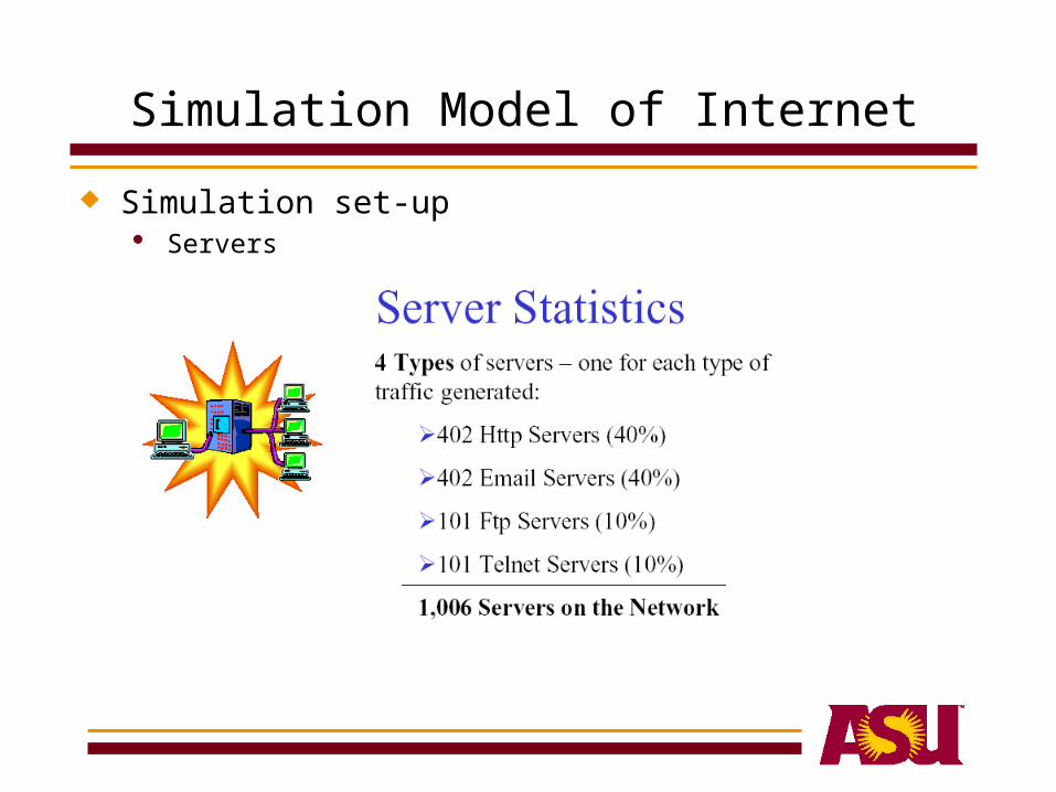
1. For all nodes with connectivity = 1, assign workstation model to 70% of nodes, server model to 30%
2. Within server nodes, assign types: 40% HTTP, 40% E-mail, 10% FTP, 10% Telnet3. For all nodes with connectivity > 16, assume ISP & assign ISP Router model
(black box ISP).4. For all remaining nodes, assign switch model5. For each ISP Router, recursively define sub-network of all nodes connected to this
router and it’s children, etc.6. Define top network as all sub-networks and the links connecting them (these are
router to router links).

Simulation Model of Internet
Research stages Stage 3
Generate java classes of Modeler Document Data Type using Oracle’s XML Class Generator for Java
Use classes to generate XML document of internet topology Import XML document to OPNET and verify links
Stage 4 Create probe models to collect metrics Collect baseline system metrics
Stage 5 Create scenarios with random failure Create scenarios with planned attack Collect metrics
Stage 6 Detect emergent network states using analytical techniques

Simulation Model of Internet
Topology 5,000 devices
32 ISP routers 1006 servers (30%)
Min subnet = 38 devices Max subnet = 441 devices
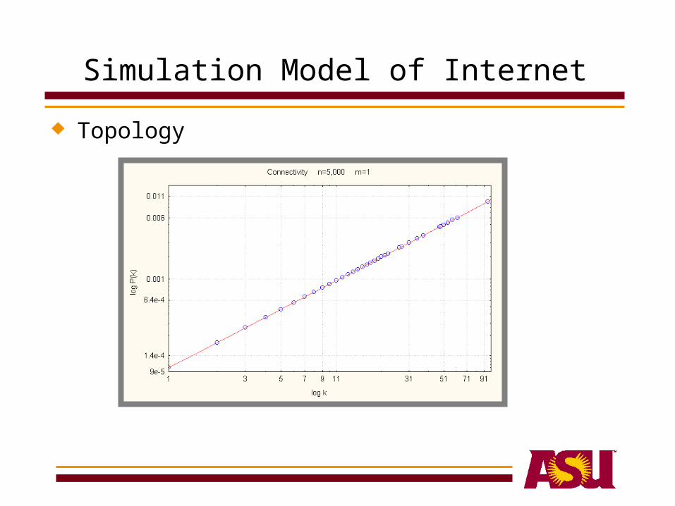
Simulation Model of Internet
Topology
Simulation Model of Internet
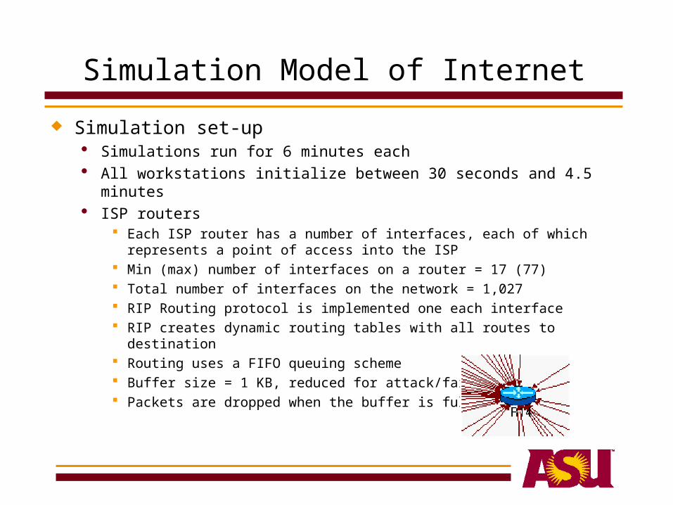
Simulation set-up Simulations run for 6 minutes each All workstations initialize between 30 seconds and 4.5 minutes ISP routers
Each ISP router has a number of interfaces, each of which represents a point of access into the ISP
Min (max) number of interfaces on a router = 17 (77) Total number of interfaces on the network = 1,027 RIP Routing protocol is implemented one each interface RIP creates dynamic routing tables with all routes to destination Routing uses a FIFO queuing scheme Buffer size = 1 KB, reduced for attack/failure Packets are dropped when the buffer is full
Simulation Model of Internet
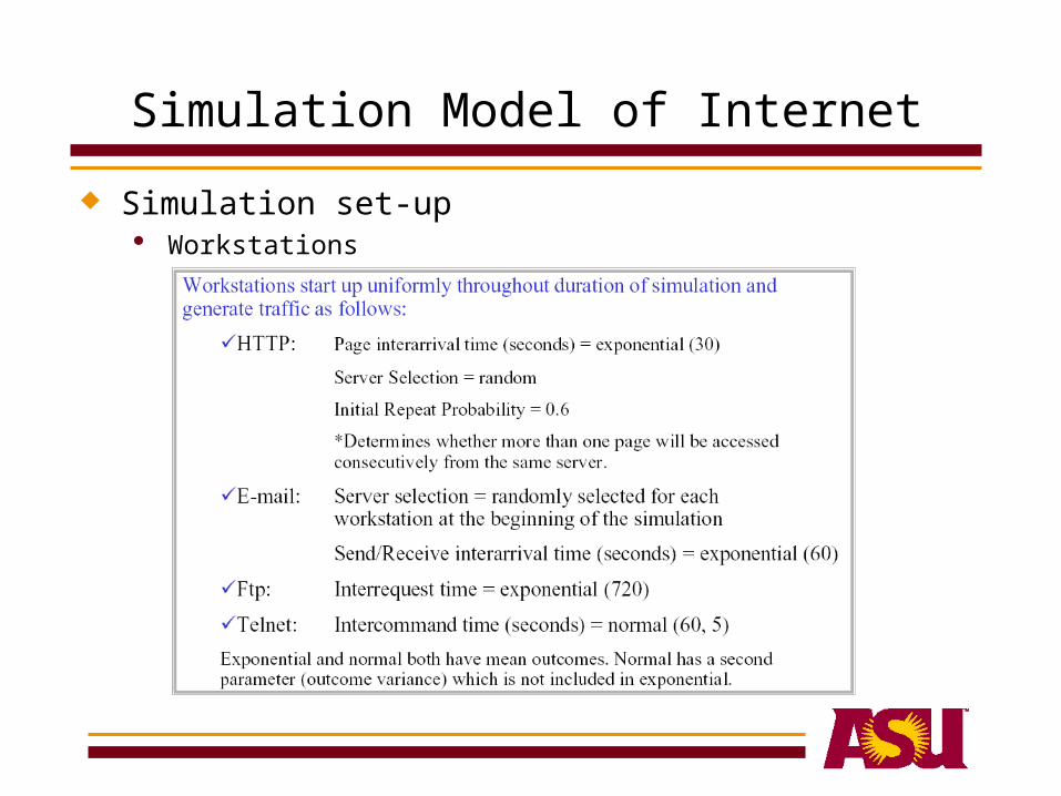
Simulation set-up Workstations
Simulation Model of Internet
Simulation set-up Servers

Simulation Model of Internet
Experimental conditions Independent variables
Under attack, a device operates at a reduced service rate Under failure, a device ceases to process traffic
Simulation Model of Internet
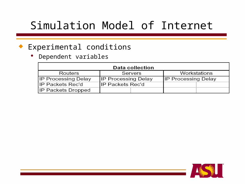
Experimental conditions Dependent variables

Simulation Model of Internet
Data collection

Simulation Model of Internet
Progress

Simulation Model of Internet
Some traffic data collected Baseline traffic
Simulation Model of Internet
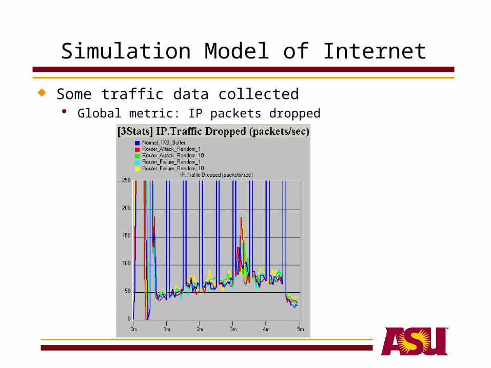
Some traffic data collected Global metric: IP packets dropped
Simulation Model of Internet
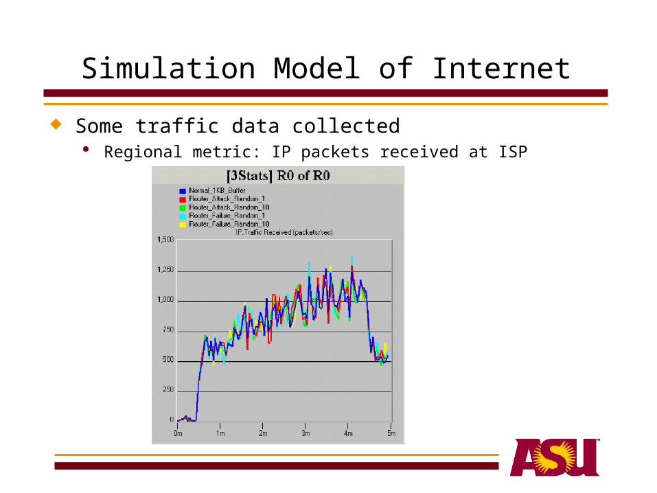
Some traffic data collected Regional metric: IP packets received at ISP

Simulation Model of Internet
Some traffic data collected Local metric: traffic received at interface

Simulation Model of Internet
Some traffic data collected Local metric: traffic dropped at interface
Simulation Model of Internet
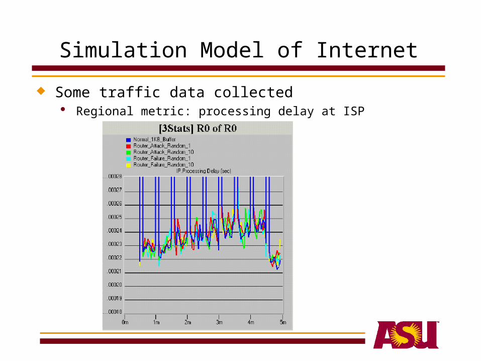
Some traffic data collected Regional metric: processing delay at ISP
Detection of Emergent Network States
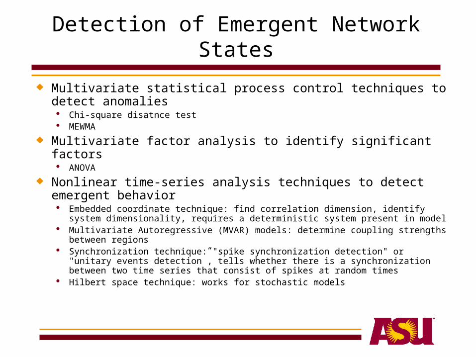
Multivariate statistical process control techniques to detect anomalies Chi-square disatnce test MEWMA
Multivariate factor analysis to identify significant factors ANOVA
Nonlinear time-series analysis techniques to detect emergent behavior Embedded coordinate technique: find correlation dimension, identify system
dimensionality, requires a deterministic system present in model Multivariate Autoregressive (MVAR) models: determine coupling strengths between
regions Synchronization technique: "spike synchronization detection" or "unitary events
detection”, tells whether there is a synchronization between two time series that consist of spikes at random times
Hilbert space technique: works for stochastic models

Regional-Level QoS Models
Regional-level systems Local area networks Administrative domains
Existing work Centralized optimization: e.g., computational grids
Allocation and scheduling are fundamental to performance Allocation of data and computation in space
Select available resources for processes Assign processes to resources Distribute processes and data
Scheduling data and computation over time Order processes on resources Order communications between processes
Objectives Promote the performance of the SYSTEM
Job schedulers: maximize throughput, minimize communication cost Resource schedulers: maximize resource utilization
Promote the performance of the INDIVIDUAL APPLICATIONS Application schedulers: optimize performance, e.g., execution time, resolution, speed, cost,
etc.

Regional-Level QoS Models
Existing work High performance schedulers
MPP (Massive Parallel Processors): produce poor performance for computational grids

Regional-Level QoS Models
Existing work High performance schedulers
Grid schedulers

Regional-Level QoS Models
Existing work High performance schedulers
Grid schedulers Program model
Represent programs in terms of their resource requirements Build a program dependency graph of phased tasks
Performance model Use the program dependency graph parameterized during execution as
performance model to predict execution time Use a generic model, e.g., execution time = computation + communication Input the data-flow program graph to expert system
Scheduling policy Choose the best among candidate schedules based on performance criteria Centralized, FCFS Load balancing

Regional-Level QoS Models
Existing work High performance schedulers
Grid schedulers Example: AppLes
Framework and a testbed
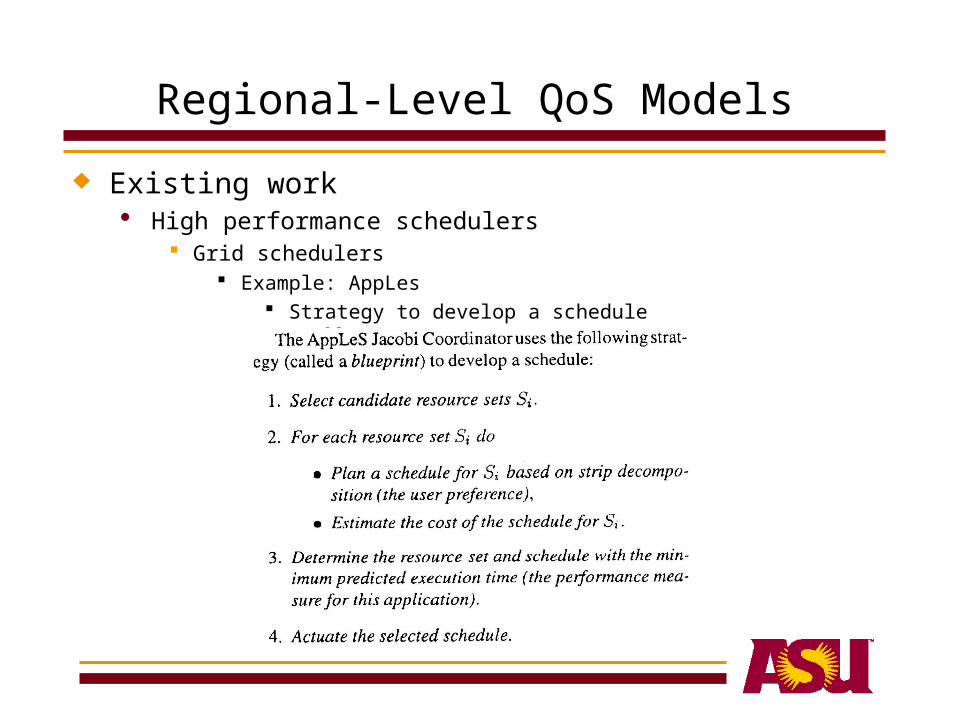
Regional-Level QoS Models
Existing work High performance schedulers
Grid schedulers Example: AppLes
Strategy to develop a schedule

Regional-Level QoS Models
Existing work High performance schedulers
Grid schedulers Example: AppLes
Cost model to evaluate strip decomposition

Regional-Level QoS Models
Existing work High performance schedulers
Grid schedulers Example: AppLes
Methods of strip decomposition

Regional-Level QoS Models
Existing work High performance schedulers
Grid schedulers Example: AppLes
Performance results

Regional-Level QoS Models
Existing work High performance schedulers
Grid schedulers Challenges
Complexity of scheduling problem Variations in deliverable resource performance due to resource
sharing Prediction of program’s resource requirements Hardware and software heterogeneity

Regional-Level QoS Models
Principles for our regional-level QoS models Simplify the scheduling problem through resource standardization,
i.e., stabilizing performance of resources to make them “standard parts”
Develop new scheduling and control strategies to achieve the objective of performance stability
Call on reserved, redundant resources to achieve performance stability under failure/attack
Make dynamic resource state available to process agents Process agents plan ahead to achieve performance objectives—a
distributed decomposition of the scheduling problem complexity Make network policies accordingly