A Comparison of Wind Turbine Load Statistics for Inflow ...€¦ · A Comparison of Wind Turbine...

A Comparison of Wind Turbine Load Statistics for

Inflow Turbulence Fields based on Conventional

Spectral Methods and Large Eddy Simulation

Chungwook Sim∗, Lance Manuel†, and Sukanta Basu‡

Efficient spatial and temporal resolution of simulated inflow velocity fields is importantin order to derive wind turbine load statistics for design. There are not many publishedstudies that have addressed the issue of such optimal space-time resolution. This study in-vestigates turbine extreme and fatigue load statistics for a utility-scale 5MW wind turbine.Load statistics, spectra, and time-frequency analysis representations are compared for var-ious alternative space and time resolutions employed in inflow turbulence field simulation.Conclusions are drawn regarding adequate resolution in space of the inflow turbulence sim-ulated on the rotor plane prior to extracting turbine load statistics. Similarly, conclusionsare drawn with regard to what constitutes adequate temporal filtering to preserve turbineload statistics. This first study employs conventional Fourier-based spectral methods forsimulating velocity fields for neutral atmospheric stability conditions.

In the second part of this study, large eddy simulation (LES) is employed with fairlycoarse resolutions in space and time, justified on the basis of the earlier Fourier-basedstochastic simulations, to again establish turbine load statistics. A comparison of extremeand fatigue load statistics is presented for the two approaches used in inflow field genera-tion. The use of LES-generated flows to establish turbine load statistics in this manner iscomputationally more expensive but the study is partly justified in order to evaluate theability of LES to be used as an alternative to the more conventional Fourier-based stochas-tic approaches. A more compelling reason for using LES is that for the stable boundarylayer, it is not possible to generate realistic inflow velocity fields except by using LES. Thisstudy sets the stage for future turbine load computations in such stable conditions wherelow-level jets, large speed and direction shears across the rotor, etc. can possibly causelarge turbine loads.

I. Introduction

Very few studies to date have addressed the issue of efficiency of spatio-temporal resolution in generatinginflow velocity fields for purposes of estimating accurate load statistics for today’s large utility-scale wind

turbines. The present study takes on this question by making use of conventional stochastic simulation ofstationary Gaussian fields using Fourier methods.

We study loads on one such utility-scale wind turbine (rated at 5 MW) that has a hub height of 90 metersand a rotor diameter of 126 meters. Our interest is in determining an acceptable frequency resolution for theinflow turbulence generation so that resulting turbine load statistics (extremes and fatigue) can be predictedwithout loss of accuracy. Spectral filtering of the “base inflow” generated at 32 Hz sampling is applied in thefrequency domain to generate samples with some intentional loss of high-frequency energy. Likewise, gridresolution on the rotor plane (which represents a square, 140 m on each side) is varied to different degrees ofcoarseness and loads studied following aeroelastic simulation. The dynamic characteristics of turbine loadsincluding the flapwise bending moment at a blade root and the fore-aft tower base bending moment arestudied.

∗Graduate Research Assistant, School of Civil Engineering, Purdue University, West Lafayette, Indiana 47907 (formerly atthe University of Texas, Austin, Texas 78712)

†Associate Professor, Dept. of Civil, Architectural, and Environmental Engineering, University of Texas, Austin, Texas78712

‡Assistant Professor, Department of Geosciences, Texas Tech University, Lubbock, Texas 79409.

1 of 15

American Institute of Aeronautics and Astronautics

48th AIAA Aerospace Sciences Meeting Including the New Horizons Forum and Aerospace Exposition4 - 7 January 2010, Orlando, Florida

AIAA 2010-829

Copyright © 2010 by Lance Manuel. Published by the American Institute of Aeronautics and Astronautics, Inc., with permission.

From the study of turbine load statistics based on stochastic simulation of inflow, we note that extremelyfine resolution in space and time is not necessary for reasonably accurate extreme and fatigue load predictionsneeded for design purposes. These same coarse spatial and temporal resolutions are next also employed instudies involving the use Large Eddy Simulation (LES) for load computations. Load statistics from stochasticsimulation and LES are then compared.

II. Spatio-Temporal Resolution in Stochastic Simulation

A Fourier-based stochastic turbulence simulation procedure was used to generate the “base inflow” forthis study. The code, TurbSim,1 was used to stochastically generate full spatio-temporal wind velocityfields. The Kaimal power spectral density (PSD) function was used for the turbulence generation. It can beexpressed as follows:

f · Sk(f)

σ2k

=4f · Lk/Vhub

(1 + 6f · Lk/Vhub)5/3

(1)

where f represents frequency in Hz; k is an index referring to the direction of the wind velocity component(k is set equal to 1, 2, or 3 for the longitudinal, lateral, and vertical components, respectively); Sk(f) is thesingle-sided power spectral density function for wind velocity component, k; σk is the standard deviation forthe wind velocity component k; Lk is the integral scale parameter for wind velocity component, k; and Vhub

is the ten-minute average hub-height longitudinal wind speed. Values for the three wind velocity componentstandard deviations and integral scale parameters are specified in the IEC 61400-1 guidelines.2

An exponential coherence function specified in the IEC 61400-1 guidelines2 was also used in this study.This function is expressed as follows:

Coh(r, f) = exp

[−12

((f · r/Vhub)

2+ (0.12r/Lc)

2)0.5

](2)

where the coherence function, Coh(r, f), is defined as the magnitude of the complex cross-spectral densityfunciton of the longitudinal wind velocity component at two spatially separated points divided by the au-tospectrum function; r is the magnitude of the projection of the separation vector between the two pointson to a plane normal to the average wind direction; and Lc is the coherence scale parameter.

The Normal Turbulence Model (NTM) with a reference turbulence intensity of 16% (corresponding toWind Turbine Site Class A) was used to generate the inflow velocity field. Using the NTM, the powerspectra, the coherence functions, and the reference turbulence intensity, full wind fields were stochasticallygenerated on a rotor plane for the wind turbine selected. A time step of 0.03125 seconds (representing 32 Hzsampling) was used to generate the “base inflow” turbulence. Table 1 summarizes various parameters andtheir values used in the inflow simulation with TurbSim. These inflow fields for three different wind speedswere filtered in the frequency domain using low-pass filters with cut-off frequencies set at 16 Hz, 8 Hz, 4 Hz,2 Hz, 1 Hz, 1/2 Hz, 1/4 Hz, and 1/8 Hz.

Table 1. Parameters and values used in inflow turbulence field simulations.

Parameters Values

Hub height (m) 90

Rotor diameter (m) 126

Hub-height wind speed (m/s) 12, 15, 18

Base inflow sampling rate (Hz) 32

Low-pass cut-off frequency (Hz) 16, 8, 4, 2, 1, 0.5, 0.25, 0.125

Grid (y × z) 13 × 13, 11 × 11, 9 × 9

Surface roughness (m) 0.1

The rotor plane of the selected 5MW turbine model3 with a rotor diameter of 126 m is represented inseparate analyses by 13×13, 11×11, and 9 ×9 grids that cover a square area of side 140 m, centered at therotor hub. The 5MW wind turbine model closely represents a utility-scale wind turbine that is currently

2 of 15


being manufactured. This model is used for our aeroelastic response simulations. The turbine is a variable-speed, collective pitch-controlled machine. Two different turbine loads are studied; these include the flapwisebending moment at a blade root (FBM) and the tower base fore-aft bending moment (TBM). Ten-minutetime series of these loads are simulated using the aeroelastic simulation tool, FAST,4 developed at NREL.

A. Filtering of Inflow Turbulence

To the base inflow (at a 32 Hz sampling rate) obtained from TurbSim, a low-pass filter was applied in thefrequency domain with cut-off frequencies defined as given in Table 1.

Power spectral densities (PSDs) computed for the various filtered longitudinal wind velocity time seriesat hub height are presented in Fig. 1. These estimated PSDs are based on an ensemble of 15 ten-minutesimulations in each case. The PSDs are shown only up to 16 Hz, the Nyquist frequency, since all the inflowtime series have an identical time step of 0.03125 seconds (32 Hz). The log-log plot shows that the inflowtime series, with or without the filtering, all follow Kolmogorov’s -5/3 power law for scaling of turbulence inthe inertial subrange. The target Kaimal power spectrum for longitudinal turbulence at hub height is alsoshown in Fig. 1; the simulated PSD for the unfiltered case matches the target spectrum well; it is slightlydeficient in power at frequencies above around 8 Hz. As increased filtering is applied, the PSDs drop atlower and lower frequencies as expected.

B. Power Spectral Density Functions for Turbine Loads

10−2

10−1

100

101

10−8

10−6

10−4

10−2

100

102

104

frequency (Hz)

Pow

er S

pect

ral D

ensi

ty [(

m/s

)2 /Hz]

−5/3 slopeTarget PSDNo filtering (32 Hz)Filtering (16 Hz)Filtering (8 Hz)Filtering (4 Hz)Filtering (2 Hz)Filtering (1 Hz)Filtering (1/2 Hz)Filtering (1/4 Hz)Filtering (1/8 Hz)

Figure 1. Target Kaimal PSD and estimated PSDs fromunfiltered and filtered simulated hub-height longitudinalvelocity time series.

Gravitational, inertial, and aerodynamic forces allcontribute to the overall loading on wind turbinecomponents.5 Gravitational loading refers, for ex-ample, to the force on blades that cause periodicloading once per revolution; these forces are experi-enced at the rotor’s rotational frequency denoted by1P (in our case, 1P corresponds to approximately0.2 Hz). Inertial loading is caused by accelerationor deceleration of the blade rotation, due to which,centrifugal forces are caused on the blades. Thiscentrifugal force has two components; one is span-wise and the other is in a normal direction. Theselatter forces influence the flapwise bending moment(FBM) on a blade. Lastly, aerodynamic loads cre-ated by the inflow affect turbine loads. It is instruc-tive to study power spectral density (PSD) func-tions of the turbine loads in order to understandthe dynamic behavior of our wind turbine.

Power spectra for FBM and TBM are presentedin Fig. 2. The loads data for these PSDs were generated from a full-field inflow on a 9×9 grid with hub-heightten-minute mean wind speed of 12 m/s. Because the natural modes of vibration for our wind turbine modelsuggest that important blade and tower vibration modes occur at frequencies below 5 Hz, log-log plots ofthe four PSDs were plotted only up to 5 Hz. (We note in passing that for the FAST simulation model usedhere, all the modes of vibration represented for the tower and blades had natural frequencies below 5 Hz.We also note that if simulation models built using other commercial codes such as ADAMS are employed,higher frequencies of vibration will likely result; however, it is our expectation that turbine loads and hencerelated fatigue and extreme loads are influenced only to a small degree by these higher frequencies.)

All the PSDs discussed here are estimated based on an ensemble of 15 simulations. Peaks in the PSDs dueto the rotational frequencies of the blade (1P = 0.2 Hz, 2P, and 3P) and other important natural frequenciesare indicated on the plots. The plots in Fig. 2 also show the PSDs derived based on filtered inflow (at variouscut-off frequencies). The 1P spectral peaks and the various resonance peaks that match natural frequenciesof the turbine blades and tower are easily identified and are all captured well even with filtering down to 1Hz.

In the FBM PSD, the presence of 1P, 2P, 3P, etc. peaks is obvious; these peaks occur due to rotationalsampling of the inflow turbulence by the moving blades. A 0.6 Hz peak is an indication of the first flapwise

3 of 15


blade bending mode. Unlike the blade loads, PSDs for the fore-aft bending moment at the tower base (TBM)in Fig. 2 show largest peaks at around 0.4 Hz (close to the 2P frequency). This frequency matches the firsttower bending natural frequency.

Studying the PSDs of the tower and blade loads helps explain why tower load statistics miss the targetto a greater degree than do the blade load statistics. The PSDs clearly show that the energy (related tovariance which is the area under the PSD) of the blade loads is relatively concentrated to a greater degreeat the low frequencies while tower loads display peaks above 2 Hz. The dominant PSD peaks for FBM arewell captured by filtered inflow; TBM spectra show less dominant peaks and some deficient energy at a fewspectral peaks.

10−2

10−1

100

10−6

10−5

10−4

10−3

10−2

10−1

100

101

102

103

104

frequency (Hz)

Po

we

r S

pe

ctra

l De

nsi

ty [

(MN

−m

)2/H

z]

No !ltering (32 Hz)

Filtering (16 Hz)

Filtering (8 Hz)

Filtering (4 Hz)

Filtering (2 Hz)

Filtering (1 Hz)

1P

2P

3P

0.6 Hz

10−2

10−1

100

10−6

10−5

10−4

10−3

10−2

10−1

100

101

102

103

104

frequency (Hz)

Po

we

r S

pe

ctra

l De

nsi

ty [

(MN

−m

)2/H

z]

No !ltering (32 Hz)

Filtering (16 Hz)

Filtering (8 Hz)

Filtering (4 Hz)

Filtering (2 Hz)

Filtering (1 Hz)

2P

0.6 Hz

1.1 Hz

1.8 Hz

3.4 Hz

Figure 2. Power spectral density function for FBM (left) and TBM (right) from inflow simulated on a 9×9grid and with a ten-minute mean wind speed of 12 m/s.

C. Turbine Load Statistics

We are interested in turbine load statistics for the various inflow time series generated. These inflow velocitytime series are generated for (i) three different hub-height mean wind speeds (12 m/s, 15 m/s, and 18 m/s);(ii) three different spatial grids/samplings on the rotor plane (13×13, 11×11, and 9×9); and (iii) eightdifferent filters (low-pass filters applied at 16 Hz, 8 Hz, 4 Hz, 2 Hz, 1 Hz, 1/2 Hz, 1/4 Hz, and 1/8 Hz).We estimate the standard deviation, the ten-minute extreme, and the equivalent fatigue load (EFL) for twodifferent turbine loads (FBM and TBM). A total of fifteen simulations were used to summarize ensembleload statistics for each load for the various inflow time series. Note that for the EFL calculations, Wohlerexponents of 10 and 3 were applied for FBM and TBM, respectively.

Ensemble standard deviation estimates of the two loads studied (but not presented here) show very slightvariation with hub-height mean wind speed. The various spatial grids and even the 9×9 grid with a 1 Hzfilter do not lead to large errors in the load standard deviations for all load types. Ensemble ten-minuteextreme load estimates show slightly decreasing trends with increase in wind speed from 12 m/s to 18 m/s.This is expected since the turbine is pitch-controlled and has rated wind speed around 11.5 m/s. Loadsare reduced for wind speeds above rated due to pitching of the blades. The various spatial grids and eventhe 9×9 grid with a 1 Hz filter do not lead to large errors in ten-minute load extremes for all load types.Ensemble equivalent fatigue load (EFL) estimates for the loads studied show increasing trends with increasein wind speed from 12 m/s to 18 m/s. These trends with wind speed are more pronounced than for theother statistics studied—namely standard deviations and ten-minute extremes. Comparing the differentspatial grids, greater variation is seen for EFL than for the other statistics. FBM EFL estimates are slightlyunderestimated with coarser spatial grids while EFL estimates for TBM are slightly overestimated withcoarser grids (see Table 2). Still, though variation due to spatial resolution of the inflow is greater for fatigueloads, again the various spatial grids and even the 9×9 grid with a 1 Hz filter do not lead to great differencesin EFL estimates for all load types.

The preceding observations suggest that it may not be necessary to employ very fine spatial sampling

4 of 15


while generating inflow turbulence to establish wind turbine loads for design. We conclude that a 9×9 spatialgrid for our rotor may be adequate for reasonably accurate load statistics. In addition, since for all the fourloads studied, the ten-minute extreme values are higher at 12 m/s wind speed than at higher wind speeds(as was also seen in a previous study6), further discussions on filtering will mostly focus on the inflow windvelocity time series with a mean hub-height wind speed of 12 m/s.

Table 2. Turbine load ensemble statistics (based on 15 simulations).

Grid, filtering FBM (kN-m) FBM (kN-m) TBM (kN-m) TBM (kN-m)

10-min extreme EFL 10-min extreme EFL

13 × 13, 32 Hz 12,979 5,656 82,295 12,585

9 × 9, 1 Hz (normalized) 0.985 0.949 0.983 1.011

D. Wavelet Analyses of Turbine Loads

As has been discussed by Kelley,7 time-frequency analysis using continuous wavelet transforms can helpstudy peaks that occur coincidentally with higher-order modes that might not be detected through spectralanalysis. Wavelet analysis of the loads data was performed to determine whether cutting off high frequenciesin the inflow turbulence would affect turbine load characteristics in any significant way. Also, non-stationarycharacteristics of loads from aeroelastic simulations such as flapwise bending loads may be lost by relyingon spectral analysis.7

Figures 3(a),(c),(e) show results of the wavelet analysis of the flapwise bending moment (FBM) resultingfrom an unfiltered inflow (13×13 grid and 32 Hz sampling) and an inflow filtered at 1 Hz on a 9×9 grid (fora hub-height mean wind speed of 12 m/s). The colorbar shows FBM values in MN-m. The x-axis showstime, while the y-axis shows the time scale of the Morlet wavelet used in the analyses. At high frequencies,the time windows are narrow; while at low frequencies, the frequency windows are narrow. In other words,the long time scale “a” on the y-axis indicates low frequencies, while the short time scale indicates highfrequencies.

The two wavelet plots demonstrate that there is almost no difference in the blade loads that results fromfiltering down to 1 Hz and using a 9×9 spatial grid for our rotor. The maximum difference in the FBMwavelet plots for the unfiltered and filtered cases is only 0.939 MN-m; peaks in time and at different scalesare recovered quite well for the filtered flows.

Figures 3(b),(d),(f) show results of the wavelet analysis of the tower base fore-aft moment (TBM) for thesame filtered versus unfiltered cases as were studied for FBM. The wavelet plots show that TBM derivedfrom unfiltered and filtered inflow also do not show great differences at low frequencies, while at higherfrequencies (a=2 sec) some of the peaks are missing for the filtered case.

E. Summary on Spatio-Temporal Filtering of Inflow in Stochastic Simulation

Inflow turbulence was generated based on conventional Fourier-based stochastic simulations. The base in-flow was filtered with various spectral cut-off frequencies to generate inflow with different spectral content,deficient in high-frequency energy. The purpose of filtering the inflow was to evaluate whether high frequen-cies are actually required in aeroelastic simulations. The filtered and unfiltered inflow fields were appliedas input to a 5MW wind turbine model. Turbine blade and tower load time series were studied. It wasfound that although power spectral density functions of the filtered inflow drop considerably with greateramounts of filtering, associated load characteristics do not change significantly. In general, for all of theloads studied, it was found that 9×9 spatial grids on the rotor plane and 1 Hz sampling could be used toestimate load statistics with reasonable accuracy. Power spectra and wavelet analyses confirmed that therewas no negligible losses from such filtering.

The findings from this study suggests that a grid spacing around one-tenth of the rotor diameter (10 m)and 1 Hz inflow data may be appropriate to generate from LES to allow for comparisons with conventionalstochastic simulation. Such spatial and temporal resolution of the inflow should also not lead to significanterrors in load statistics.

5 of 15


(a) FBM (unfiltered) (b) TBM (unfiltered)

(c) FBM (filter: 1 Hz) (d) TBM (filter: 1 Hz)

(e) Difference of FBM (f) Difference of TBM

Figure 3. Wavelet analysis of turbine blade and tower loads

6 of 15


III. Large Eddy Simulation for Neutrally Stable Inflow Turbulence

Based on the preceding discussion, we determined adequate temporal and spatial sampling values thatmay be used for stochastic simulation of inflow wind velocity fields for wind turbine loads analysis. Weassume that similar spatio-temporal resolution may be employed in large eddy simulation (LES) of inflowfields and that turbine loads based on LES and stochastic simulation may then be directly compared. WhileLES preserves realistic atmospheric boundary layer characteristics by directly solving the nonlinear Navier-Stokes equation and the conservation of mass equation, due to the computational effort required in suchsimulations, less computationally intensive stochastic simulations based on Fourier techniques are commonlyused in the design of wind turbines. In contrast, however, stochastic simulations have limitations especiallyin modeling the stratified stable boundary layer (SBL) which is often accompanied by high wind shear andlow-level jets and potentially large turbine loads. The present study is being undertaken prior to applyingLES in SBL simulations; we seek first to evaluate wind turbine load statistics for ideal neutral conditionsthat can be simulated using stochastic techniques and compared with those based on LES-generated inflow.The theoretical background on the use of LES is summarized very briefly here. We briefly demonstrate, too,how the inflow turbulence is generated using LES with fractal interpolation which is introduced to enhancethe deficient high-frequency energy.

A. Governing Equations of Large Eddy Simulation

Large eddy simulation (LES) is at present the most efficient technique available for high Reynolds numberflow simulations, such as for atmospheric boundary layer (ABL) simulations, in which the larger scales ofmotion are resolved explicitly and the smaller ones are modeled. Over the past three decades, the field of LESfor the ABL has evolved quite dramatically; LES has enabled researchers to probe various boundary layerflows by generating unprecedented high-resolution four-dimensional turbulence data. As a consequence, wehave gained a better understanding of some fairly complex ABL phenomena. In rotation-influenced ABLs,the equations for the conservation of momentum (using the Boussinesq approximation) and temperature are:

∂ui

∂t+

∂(uiuj)

∂xj= − ∂p

∂xi− ∂τij

∂xi+ δi3g

(θ −⟨θ⟩)

θ0+ fcεij3uj + Fi (3)

∂θ

∂t+

∂(uj θ

)∂xj

= − ∂qj∂xj

(4)

where t refers to time; xj is the spatial coordinate in the direction, j; uj is the velocity component in thedirection, j; θ is potential temperature; θ0 is the reference surface potential temperature; p is the dynamicpressure; δi3 is the Kronecker delta; ϵij3 is the alternating unit tensor; g is the gravitational acceleration; fcis the Coriolis parameter; and Fi is a forcing term (e.g., geostrophic wind).

Molecular dissipation and diffusion are neglected here since the Reynolds number of the ABL is very highand no near-ground viscous processes are resolved. Note that ⟨.⟩ is used to define a horizontal plane average;also the tilde (i.e.,“∼”) above some variables in Eqs. 3 and 4 denotes a spatial filtering operation, using afilter of characteristic width, ∆f . These filtered equations are now amenable to numerical solution on a gridof mesh size, ∆g, considerably larger than the smallest scale of turbulent motion (the so-called Kolmogorov

scale). The effects of the unresolved scales (smaller than ∆f ) on the evolution of ui and θ appear in thesubgrid-scale (SGS) stress, τij (in Eq. 3) and the SGS flux, qj (in Eq. 4), respectively; these are defined as

follows: τij = uiuj − uiuj and qj = uiθ− uiθ. Note that the SGS stress and flux quantities are unknown andmust be parameterized (using a SGS model) as a function of the resolved velocity and temperature fields.Eddy viscosity models, the most popular SGS models, use the “gradient hypothesis” and formulate the SGSstress tensor (the deviatoric part) as follows:8,9

τij −1

3τkkδij = −2νtSij (5)

where Sij is the resolved strain rate tensor and νt denotes the eddy viscosity.From a dimensional analysis, νt can be interpreted as the product of a characteristic velocity scale and a

characteristic length scale.9 Different eddy-viscosity formulations basically use different velocity and length

7 of 15


scales. The most popular eddy viscosity formulation is the Smagorinsky model:8

νt = (Cs∆f )2∣∣∣S∣∣∣ (6)

where Cs is the so-called Smagorinsky coefficient, which is adjusted empirically or dynamically to accountfor shear, stratification, and grid resolution, and |Sij | is the magnitude of the resolved strain rate tensor.

Similar to the SGS stresses, eddy-diffusivity models are used for the SGS heat fluxes as follows:

qi = −νht∂θ

∂xi= − νt

PrSGS

∂θ

∂xi(7)

where PrSGS is the SGS Prandtl number.The values of the Smagorinsky-type SGS model parameters, Cs and PrSGS , are well established for

homogeneous isotropic turbulence.10 However, the value of Cs is expected to decrease with increasing meanshear and stratification. This expectation has been confirmed by various recent field studies. In orderto account for shear and stratification, application of the traditional eddy-viscosity model in LES of ABLflows (with strong shear near the ground and temperature-driven stratification) has traditionally involvedthe use of various types of wall-damping functions and stability corrections, which are either based on thephenomenological theory of turbulence or empirically derived from observational data. Similarly, a prioriprescriptions exist also in the case of eddy-diffusivity SGS models.

An alternative approach is to use the “dynamic” SGS modeling approach. In this approach, one com-putes the value of the unknown SGS coefficients (e.g., Cs in the Smagorinsky-type eddy-viscosity models)dynamically at every time and every position in the flow. By looking at the dynamics of the flow at twodifferent resolved scales and assuming scale similarity as well as scale invariance of the model coefficient, onecan optimize its value.10,11 Thus, the dynamic model avoids the need for a priori specification and tuningof the coefficient because it is evaluated directly from the resolved scales in an LES. Recently, Basu andPorte-Agel12 proposed a refined dynamic modeling approach (called the “locally-averaged scale-dependentdynamic” or LASDD SGS modeling approach) for ABL simulations. The potential of the LASDD SGSmodel was demonstrated in large-eddy simulations of the neutral boundary layer,13 of the stable boundarylayer,12 and of a complete diurnal cycle.14 In the present study, we utilize the LASDD model to generateneutral boundary layer inflow conditions for wind turbine load calculations using an aeroelastic model.

B. LES and Stochastic Simulation of Inflow Turbulence

In atmospheric large eddy simulations, idealized or observed soundings (i.e., 1-D vertical profiles) of windspeed and other environmental variables (such as temperature, moisture, etc.) in conjunction with small-scale 3-D perturbations (random noise) are typically used to generate initialization fields. With the help ofthe Navier-Stokes equations (Eq. 3), these fields are then evolved in time under the constraints of certainlarge-scale forcing terms (e.g., geostrophic wind) and boundary conditions (e.g., prescribed land-surfacetemperature is often used as the lower boundary condition). Usually, it takes about an hour of simulation(depending on the characteristics of the boundary layer to be simulated) to generate realistic turbulence(e.g., for reasonable representation of the inertial range of spectra). However, it can take a few hours ofsimulation to generate quasi-steady state boundary layer conditions. For realistic neutral boundary layersimulations, one needs to run an LES code for O(12) hours to reach quasi-steady state conditions.

High-resolution LES runs are computationally very expensive, especially for durations of O(12) physicalhours. For this reason, in the present research study, we carry out the simulations in two phases (see Fig. 4).In Phase I, coarse runs (with a grid resolution of 20 m) of 12-hour duration are performed using a time stepof 0.2 seconds. Then, in Phase II, the final 3-D fields from the phase I simulations are used as initial fieldsand new simulations are run for 30 minutes (with a time step of 0.1 seconds). In order to create higherresolution (finer than 20 m) LES data, we first apply a cubic spline interpolation to the final 3-D fieldsof the Phase I simulations to produce 13.3 m resolution initial fields. Full-field wind files for 3-D velocitycomponents are output from the last 15 minutes of these 30-minute Phase II simulations at a frequency of2.5 Hz (i.e., every 0.4 seconds). For both phases of our simulations, we kept a fixed domain size of 800 m ×800 m × 1,260 m.

Figure 5 shows a 180 m × 180 m (y-z plane) slice of the longitudinal velocity (U) taken at one timeinstant from the last 15-minute time history segment of the simulated wind field (with a grid resolution of

8 of 15


13.3 m); also shown are the 15-min time series for U versus vertical elevation (z) for points laterally separatedby 150 m. In this study, we systematically varied geostrophic winds (a large-scale forcing term related tomesoscale pressure gradient force) to obtain various hub-height wind speeds.

Coarse (40 x 40 x 64)

Fine

(64 x 64 x 96)

0 hr 12 hr 12:30 hr

Interpolate

Figure 4. Two phases of the LES flow generation.

Figure 5. Slice of the last 15 minutes generated fromLES: Phase II longitudinal velocity wind field

In addition, three sets of LES were generated foreach geostrophic wind case. After generating thesewind fields, the 800 m × 800 m × 1,260 m domainwas sliced into 5 pieces in the y direction yieldinga total number of 15 cases covering (lateral) rotorplanes. In addition, since the w-components weregenerated in a staggered form vertically where theywere spaced between the vertical grid points of theu and v-components, the w-components were inter-polated to the grid points of u and v-components.Then, the entire turbulence field was interpolatedto the same grid points that were used in gener-ating the NBL inflow with stochastic simulations.In order to provide neutral boundary layer flowsfrom stochastic simulations whose effects on tur-bine loads could be directly compared with theneutral boundary layer flows generated from LES,the Fourier-based stochastic turbulence simulation

code, TurbSim, was used together with target turbulence power spectra and coherence functions (the Kaimalmodel). The rotor plane of the selected 5MW turbine, with a rotor diameter of 126 m, was represented as a13 × 13 grid that covers a square area of side 160 m, centered at the rotor hub. A time-step of 0.4 secondswas used in the NBL flow simulations to match the time step from LES. Note that the resultant of u andv-component wind speed at hub height (90 m) for the LES case was matched to the hub-height mean windspeed of the TurbSim simulations. A total of 15 simulations were produced and compared with the LESresults.

−60

−40

−20

0

20

40

60

20406080100120140160

0.9

1

1.1

1.2

1.3

1.4

1.5

Lateral grid points (m)

Vertical grid points (m)

Var

ianc

e on

Rot

or P

lane

TurbSimLES

Figure 6. 3-D Variance of inflow turbulence across therotor plane

Figure 6 shows a 3-D plot of variance of inflowturbulence across the rotor plane. The target vari-ance in TurbSim is treated as constant over theentire rotor plane although this is not physicallyrealistic. Large eddy simulation generates turbu-lence at the surface and transports it upwards inneutral flows. As a result, variance and fluxes arehigher near the surface and will decrease monotoni-cally with height. Moreover, the variance and fluxesshould be zero at the top of boundary layers (BL).Figure 6 clearly demonstrates that LES is capturingthe correct behavior of BL characteristics. Near thehub height (90 m) of our turbine model, the vari-ance of LES and TurbSim match reasonably well.However, while the variance from TurbSim is con-stant over the entire rotor plane, the variance fromLES has higher values close to the ground (20 m)and lower values above 90 m.

To evaluate the LES of neutral boundary flow (NBL) by comparing the loads from LES flows with thoseform TurbSim (stochastic simulator), we would like to modify any differences in inflow in reasonable ways.Though there are noted differences in inflow variance from LES versus TurbSim over the rotor plane, this

9 of 15


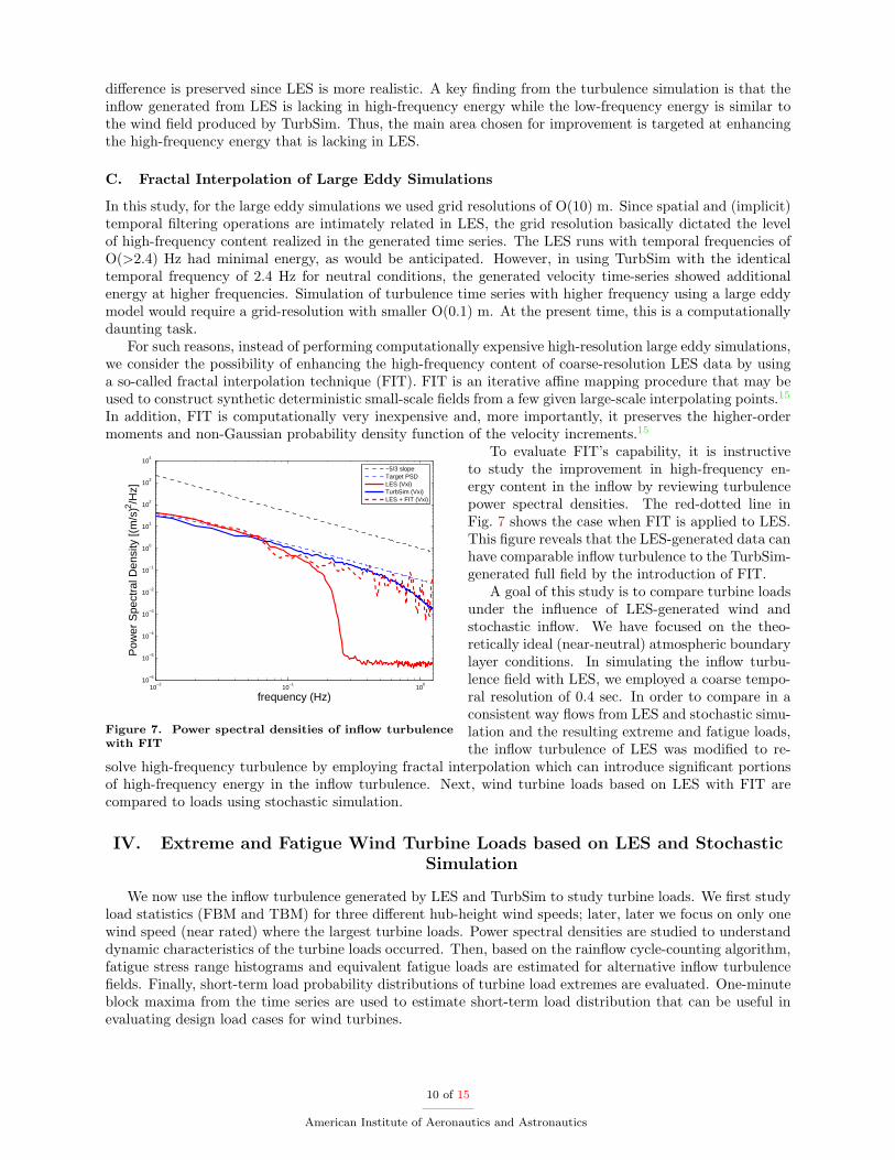
difference is preserved since LES is more realistic. A key finding from the turbulence simulation is that theinflow generated from LES is lacking in high-frequency energy while the low-frequency energy is similar tothe wind field produced by TurbSim. Thus, the main area chosen for improvement is targeted at enhancingthe high-frequency energy that is lacking in LES.

C. Fractal Interpolation of Large Eddy Simulations

In this study, for the large eddy simulations we used grid resolutions of O(10) m. Since spatial and (implicit)temporal filtering operations are intimately related in LES, the grid resolution basically dictated the levelof high-frequency content realized in the generated time series. The LES runs with temporal frequencies ofO(>2.4) Hz had minimal energy, as would be anticipated. However, in using TurbSim with the identicaltemporal frequency of 2.4 Hz for neutral conditions, the generated velocity time-series showed additionalenergy at higher frequencies. Simulation of turbulence time series with higher frequency using a large eddymodel would require a grid-resolution with smaller O(0.1) m. At the present time, this is a computationallydaunting task.

For such reasons, instead of performing computationally expensive high-resolution large eddy simulations,we consider the possibility of enhancing the high-frequency content of coarse-resolution LES data by usinga so-called fractal interpolation technique (FIT). FIT is an iterative affine mapping procedure that may beused to construct synthetic deterministic small-scale fields from a few given large-scale interpolating points.15

In addition, FIT is computationally very inexpensive and, more importantly, it preserves the higher-ordermoments and non-Gaussian probability density function of the velocity increments.15

10−2

10−1

100

10−6

10−5

10−4

10−3

10−2

10−1

100

101

102

103

104

frequency (Hz)

Pow

er S

pect

ral D

ensi

ty [(

m/s

)2 /Hz]

−5/3 slopeTarget PSDLES (Vxi)TurbSim (Vxi)LES + FIT (Vxi)

Figure 7. Power spectral densities of inflow turbulencewith FIT

To evaluate FIT’s capability, it is instructiveto study the improvement in high-frequency en-ergy content in the inflow by reviewing turbulencepower spectral densities. The red-dotted line inFig. 7 shows the case when FIT is applied to LES.This figure reveals that the LES-generated data canhave comparable inflow turbulence to the TurbSim-generated full field by the introduction of FIT.

A goal of this study is to compare turbine loadsunder the influence of LES-generated wind andstochastic inflow. We have focused on the theo-retically ideal (near-neutral) atmospheric boundarylayer conditions. In simulating the inflow turbu-lence field with LES, we employed a coarse tempo-ral resolution of 0.4 sec. In order to compare in aconsistent way flows from LES and stochastic simu-lation and the resulting extreme and fatigue loads,the inflow turbulence of LES was modified to re-

solve high-frequency turbulence by employing fractal interpolation which can introduce significant portionsof high-frequency energy in the inflow turbulence. Next, wind turbine loads based on LES with FIT arecompared to loads using stochastic simulation.

IV. Extreme and Fatigue Wind Turbine Loads based on LES and StochasticSimulation

We now use the inflow turbulence generated by LES and TurbSim to study turbine loads. We first studyload statistics (FBM and TBM) for three different hub-height wind speeds; later, later we focus on only onewind speed (near rated) where the largest turbine loads. Power spectral densities are studied to understanddynamic characteristics of the turbine loads occurred. Then, based on the rainflow cycle-counting algorithm,fatigue stress range histograms and equivalent fatigue loads are estimated for alternative inflow turbulencefields. Finally, short-term load probability distributions of turbine load extremes are evaluated. One-minuteblock maxima from the time series are used to estimate short-term load distribution that can be useful inevaluating design load cases for wind turbines.

10 of 15


A. Turbine Load Statistics

We study turbine load statistics for the various inflow fields generated by different simulation techniques.These inflow fields are based on three different simulation models: LES, LES with FIT, and TurbSim; andthree different ten-minute mean hub-height wind speeds: 12 m/s, 15 m/s, and 17 m/s. We are interested inthe ten-minute extreme, the ten-minute mean, and the standard deviation for the two different turbine loads(FBM and TBM). A total of fifteen simulations were used for the turbine load calculations with each of theinflow fields. The results of these simulations are represented in box plots. These plots are also referred toas box-whisker diagrams.16 Quartiles that represent the 25% (lower quartile), 50% (median), and the 75%(upper quartile) are extracted from the data set; these quartiles form the box. The box-whisker plots forFBM and TBM statistics illustrated in Figs. 8 and 9, respectively, identify the quartiles as well as maximumand minimum values of the relevant statistic (mean, standard deviation, or ten-minute maximum) from 15simulations. Each figure summarizes statistics for the three inflow options (LES, LES + FIT, TurbSim) andthe three wind speeds. The red box represents the LES case; the green box represents the case for LESinflow with fractal interpolation; and the blue box represents the TurbSim case.

4

5

6

7

8

9

10

12 m/s

Mea

n of

FB

M (

MN

−m

)

4

5

6

7

8

9

10

15 m/s4

5

6

7

8

9

10

17 m/s1

1.1

1.2

1.3

1.4

1.5

1.6

12 m/s

Sta

ndar

d D

evia

tion

of F

BM

(M

N−

m)

1

1.1

1.2

1.3

1.4

1.5

1.6

15 m/s1

1.1

1.2

1.3

1.4

1.5

1.6

17 m/s8.5

9

9.5

10

10.5

11

11.5

12

12.5

13

12 m/s

10−

min

Ext

rem

e of

FB

M (

MN

−m

)

8.5

9

9.5

10

10.5

11

11.5

12

12.5

13

15 m/s8.5

9

9.5

10

10.5

11

11.5

12

12.5

13

17 m/s

Figure 8. Box-whisker plots summarizing ensemble statistics for FBM based on 15 simulations: mean (left);standard deviation (middle); ten-minute maximum (right).

30

35

40

45

50

55

60

65

12 m/s

Mea

n of

TB

M (

MN

−m

)

30

35

40

45

50

55

60

65

15 m/s30

35

40

45

50

55

60

65

17 m/s3.5

4

4.5

5

5.5

6

6.5

7

12 m/s

Sta

ndar

d D

evia

tion

of T

BM

(M

N−

m)

3.5

4

4.5

5

5.5

6

6.5

7

15 m/s3.5

4

4.5

5

5.5

6

6.5

7

17 m/s40

45

50

55

60

65

70

75

80

12 m/s

10−

min

Ext

rem

e of

TB

M (

MN

−m

)

40

45

50

55

60

65

70

75

80

15 m/s40

45

50

55

60

65

70

75

80

17 m/s

Figure 9. Box-whisker plots summarizing ensemble statistics for TBM based on 15 simulations: mean (left);standard deviation (middle); ten-minute maximum (right).

The loads are seen to have higher standard deviations with increasing wind speed. Ten-minute extremeloads and mean values for the two loads and for the different inflow simulation options suggest that theinflow conditions associated with the hub-height wind speed of 12 m/s bring about the largest loads. Theseresults are understandable since turbine loads generally decrease as wind speeds exceed the rated wind speeddue to pitch control actions. In the following discussions, we will focus only on loads from inflow fields witha hub-height mean wind speed of 12 m/s.

B. Power Spectral Density Functions of Turbine Loads

Power spectral densities (PSD) of turbine loads that result from inflow turbulence generated by LES, LESwith FIT, and TurbSim are plotted in Figure 10.

11 of 15


102

10 1

100

10 6

10 5

10 4

10 3

10 2

10 1

100

101

102

103

104

frequency (Hz)

Pow

er S

pect

ral D

ensi

ty [(

MN

m

)2 /Hz]

LES (FBM)TurbSim (FBM)LES + FIT (FBM)

1P

2P

0.6 Hz

3P

1.1 Hz

-

102

10 1

100

10 6

10 5

10 4

10 3

10 2

10 1

100

101

102

103

104

frequency (Hz)

Pow

er S

pect

ral D

ensi

ty [(

MN

m

)2 /Hz]

LES (TBM)TurbSim (TBM)LES + FIT (TBM)

2P 0.6 Hz

3P

1.1 Hz

-

Figure 10. Power spectral density function for FBM (left) and TBM (right) for different inflow simulationoptions with a hub-height ten-minute mean wind speed of 12 m/s.

The peaks at 0.6 Hz and 1.1 Hz in the spectra match the natural frequencies of the 1st mode of flapwisebending moment and the edgewise bending moment of the blades. On studying the FBM power spectra inFig. 10, one can see that although there is some energy loss in the PSD for LES and PSD for LES with FITat low frequencies, the dominant (1P) peak matches that in the PSD for TurbSim quite well, even withoutapplying fractal interpolation. There is slight energy loss at low frequencies but all the peaks shown (suchas at 1P, 2P, 3P, etc.) are quite close for all the inflow simulation options.

While the blade loads under inflow turbulence generated by LES preserved the important peaks in thePSDs reasonably well, the TBM power spectrum with LES inflow misses the spectral peak at the naturalfrequency of the 1st tower fore-aft bending mode at 0.4 Hz (around 2P) as can be seen in Fig. 10. Since thisfirst peak makes an important contribution to the overall energy content, this deficit can lead to errors intower load estimation. However, fractal interpolation recovers much of the missing energy between 0.4 Hzand 0.8 Hz.

C. Fatigue Load Estimation

Stress range histograms can be established from time series of wind turbine loads by various means includingthe rainflow cycle counting algorithm,17 which is a commonly used method used to count the number ofcycles in an irregular load or stress time history. Fatigue damage in any single cycle is proportional to

the stress range amplitude, S, to the mth power, where m is the Wohler exponent. In variable-amplitude

stress cycles, it is convenient to define an equivalent fatigue load (EFL) which represents the mth root ofthe expected value of Sm. The expected value of Sm, in turn, is obtained by establishing the empiricaldistribution of the stress ranges that is achieved by rainflow cycle counting. Note that the EFL measurein combination with the total number of cycles counted is to be interpreted as that derived stress rangeamplitude (from the variable-amplitude stress history) that causes the same amount of damage as the samenumber of cycles of a constant-amplitude stress history would.

To obtain equivalent fatigue load (EFL) estimates for the wind turbine, Wohler exponents equal to 3and 10, respectively, are assumed for the steel tower (i.e., for TBM) and for the blades composed of fibercomposite material (i.e., for FBM).

From each of the 15 simulated time series, load cycles were counted using the rainflow cycle countingalgorithm. The counted stress cycles were translated into histograms and the equivalent fatigue load (EFL)and effectve number of cycles (N)was also computed. Figures 11 and 12 show fatigue stress range histogramsof FBM and TBM, respectively. Also indicated are EFL and N values.

Stress range histograms based on LES flows are slightly lacking in some of the stress cycle bins comparedto the those from the TurbSim flows. It is evident that fractal interpolation helps by filling in some of themissing cycles. Fatigue damage on the blades is somewhat larger for the LES inflow than for the TurbSiminflow. Fractal interpolation, with the additional high-frequency energy, increases the fatigue damage even

12 of 15


0 1 2 3 4 5 6 7 8 9 100

0.2

0.4

0.6

0.8

1

1.2

1.4

1.6

1.8

2

Stress Range of FBM (MN−m)

Cyc

le C

ount

s, lo

g10

Equivalent Fatigue Loads: 3.487 units for N=306.5

0 1 2 3 4 5 6 7 8 9 100

0.2

0.4

0.6

0.8

1

1.2

1.4

1.6

1.8

2


Cyc

le C

ount

s, lo

g10

Equivalent Fatigue Loads: 4.41 units for N=247

0 1 2 3 4 5 6 7 8 9 100

0.2

0.4

0.6

0.8

1

1.2

1.4

1.6

1.8

2


Cyc

le C

ount

s, lo

g10


Figure 11. Fatigue stress range histograms based on 15 simulations for FBM (wind speed = 12 m/s): TurbSim(left); LES (middle); LES + FIT (right).

0 5 10 15 20 25 30 35 400

0.2

0.4

0.6

0.8

1

1.2

1.4

1.6

1.8

2

Stress Range of TBM (MN−m)

Cyc

le C

ount

s, lo

g10


0 5 10 15 20 25 30 35 400

0.2

0.4

0.6

0.8

1

1.2

1.4

1.6

1.8

2


Cyc

le C

ount

s, lo

g10


0 5 10 15 20 25 30 35 400

0.2

0.4

0.6

0.8

1

1.2

1.4

1.6

1.8

2


Cyc

le C

ount

s, lo

g10

Equivalent Fatigue Loads: 8.185 units for N=328.5

Figure 12. Fatigue stress range histograms based on 15 simulations for TBM (wind speed = 12 m/s): TurbSim(left); LES (middle); LES + FIT (right).

more relative to the TurbSim inflow. However, TBM EFL estimate for LES inflow was about 20% smallerthan the EFL value based on TurbSim inflow before FIT was applied; damage was about 40% smaller. Afterfractal interpolation, the equivalent fatigue load and damage were comparable with that from TubSim inflow,differing by less than 10%.

D. Long-term Load Estimation

The International Electrotechnical Commission (IEC) standard2 for the design of wind turbines includes aload case (for an ultimate limit state) that requires estimation of a 50-year return period load. In orderto estimate this rare load from a limited number of simulations, one needs to use statistical extrapolationto predict this rare long-term load. Design Load Case (DLC) 1.1 in the IEC standard requires inflowturbulence under near-neutral atmospheric conditions and with specified turbulence intensity values thatshould be simulated with a normal turbulence model (NTM). The ten-minute average hub-height windspeed is treated as a single random variable representing the environment. In addition, to obtain loads foraddressing DLC 1.1, the IEC standard requires one to perform aeroelastic simulations for the entire power-producing wind speed range. In this study, our simulations are limited to three specific wind speeds sincethe objective of this study was only to evaluate alternate inflow simulation methods. As a result, we onlycompute “short-term” load distributions for the wind speeds studied; we do not attempt a full long-termload extrapolation.

In order to predict short-term load extremes from ten-minute time series, one can use the peak-over-threshold (POT) method or one can extract global (ten-minute) maxima or block maxima (maxima over fixedintervals shorter than ten minutes). Agarwal18 demonstrated that the three alternative extreme models—peak-over-threshold(POT), global maxima, and block maxima—all give comparable load distributions if asufficient number of simulations are available to obtain the distribution tails. The present study is basedon a limited number of simulations; hence, we use one-minute block maxima to define our extreme load

13 of 15


statistics. Under the assumption that these one-minute maxima are independent of each other, the short-term ten-minute maximum (L) distribution may be obtained for any wind speed V = v from the short-termblock maxima (Lblock). In terms of the probability of exceedance of any load level, l, the short-term globalmaxima distribution may be expressed as follows:

P (L > l|V = v) = 1− [1− P (Lblock > l|V = v)]n (8)

Accounting for the different values of V , the long-term distribution on L can be obtained as follows:

P (L > l) =

Vout∫Vin

P (L > l |V = v)fV (v)dv (9)

where fV (v) is the wind speed probability density function which is usually taken to be a Weibull or Rayleighdensity function.

9 10 11 12 13 14 15 16 17 1810

−4

10−3

10−2

10−1

100

FBM (MN−m)

Exc

eeda

nce

Pro

babl

ility

in 1

−m

in

LES: 1−min Block MaximaLES + FIT: 1−min Block MaximaTurbSim: 1−min Block Maxima

50 55 60 65 70 75 80 85 90 95 10010

−4

10−3

10−2

10−1

100

TBM (MN−m)

Exc

eeda

nce

Pro

babl

ility

in 1

−m

in

LES: 1−min Block MaximaLES + FIT: 1−min Block MaximaTurbSim: 1−min Block Maxima

Figure 13. Short-term probability distribution of wind turbine loads for a wind speed of of 12 m/s for FBM(left) and TBM (right).

Figure 13 shows the short-term distribution for FBM and TBM loads. For the FBM loads, fractalinterpolation leads to no change in the load distribution obtained using LES. The difference between LESand TurbSim predictions of the 80th percentile ten-minute maximum value (or, equivalently, of the loadassociated with a 0.022 non-exceedance probability in 1 minute) is approximately 10% for this load. Forthe TBM loads, the LES distribution matches that from TurbSim while fractal interpolation introduces adeviation in the tail. It appears that excessive high-frequency energy introduced by FIT causes large loadsin a few simulations that directly influences the distribution tails. Note, however, that the short-term loadsdistributions presented here are based only on a limited number of simulations; additional simulations mightbe warranted to establish stable extreme distribution tails.

V. Conclusions

Turbine loads under inflow turbulence generated by different simulation techniques were compared. Inflowturbulence for a neutrally stable boundary layer generated by conventional stochastic simulation, large-eddysimulation, and large-eddy simulation with fractal interpolation was considered. Load statistics were studiedto understand the characteristics of turbine loads at different hub-height wind speeds. The hub-height windspeed of 12 m/s had the largest loads compared to the wind speeds of 15 m/s or 17 m/s. Fractal interpolationwas helpful for recovering energy deficit at high frequencies in large-eddy simulations. Fatigue loads andstress range histograms were also studied; again fractal interpolation improves the stress cycle histogramsfrom LES versus stochastic simulation. Short-term load distributions of turbine loads were studied using1-min block maxima; these distributions from stochastic simulation and LES were reasonably consistent witheach other.

14 of 15


Based on the various turbine load studies conducted, it is concluded that large-eddy simulations withfractal interpolation can generate turbine loads that are comparable with the stochastic simulation results.For fatigue and ultimate limit states, LES with FIT is an attractive alternative to stochastic simulation.Having demonstrated its effectiveness as has been done here, future work is planned where LES with FITwill be employed to assess loads on turbines in the stable boundary layer where stochastic simulation is nolonger possible.

Acknowledgements

The authors gratefully acknowledge the financial support provided by Sandia National Laboratories (Con-tract Nos. 681008 and 743358), by the Texas Higher Education Coordinating Boards Norman HackermanAdvanced Research Program (Grant No. 003658-0100-2007), and by the National Science Foundation (GrantNos. ATM-0748606, CMS-0449128).

References

1Jonkman, B., “TurbSim User’s Guide: Version 1.50,” Tech. Rep. NREL/TP-500-46198, National Renewable EnergyLaboratory, Golden, CO, 2009.

2International Electrotechnical Commission, Wind Turbines - Part 1: Design Requirements, IEC-61400-1, Edition 3.0,2007.

3Jonkman, J., Butterfield, S., Musial, W., and Scott, G., “Definition of a 5MW Reference Wind Turbine for OffshoreSystem Development,” Tech. Rep. NREL/TP-500-38060, National Renewable Energy Laboratory, Golden, CO, 2007.

4Jonkman, J. and Buhl, M., “FAST User’s Guide,” Tech. Rep. NREL/EL-500-38230, National Renewable Energy Labo-ratory, Golden, CO, 2005.

5Hansen, M., Aerodynamics of Wind Turbines, Earthscan Publications Ltd., 2nd ed., 2008.6Fogle, J., Agarwal, P., and Manuel, L., “Towards an Improved Understanding of Statistical Extrapolation for Wind

Turbine Extreme Loads,” Wind Energy, Vol. 11, 2008, pp. 613–635.7Kelley, N., Osgood, R., Bialasiewicz, J., and Jakubowski, A., “Using Wavelet Analysis to Assess Turbulence/Rotor

Interactions,” Wind Energy, Vol. 3, 2000, pp. 121–134.8Smagorinsky, J., “General Circulation Experiments with the Primitive Equations,” Monthly Weather Review , Vol. 91,

1963, pp. 99–164.9Geurts, B., Elements of Direct and Large-Eddy Simulation, Edwards, 2003.

10Lilly, D., “A Proposed Modification of the Germano Subgrid-scale Closure Method,” Physics of Fluids A, Vol. 4, 1992,pp. 633–635.

11Germano, M., Piomelli, U., Moin, P., and Cabot, W., “A Dynamic Subgrid-scale Eddy Viscosity Model,” Physics ofFluids A, Vol. 3, 1991, pp. 1760–1765.

12Basu, S. and Porte-Agel, F., “Large-Eddy Simulation of Stably Stratified Atmospheric Boundary Layer Turbulence: aScale-Dependent Dynamic Modeling Approach,” Journal of the Atmospheric Sciences, Vol. 63, 2006, pp. 2074–2091.

13Anderson, W., Basu, S., and Letchford, C., “Comparison of Dynamic Subgrid-scale Models for Simulations of NeutrallyBuoyant Shear-driven Atmospheric Boundary Layer Flows,” Enviornmental Fluid Mechanics, Vol. 7, 2007, pp. 195–215.

14Basu, S., Vinuesa, J.-F., and Swift, A., “Dynamic LES Modeling of a Diurnal Cycle,” Journal of Applied Meteorologyand Climatology, Vol. 47, 2008, pp. 1156–1174.

15Basu, S., Foufoula-Georgiou, E., and F. Porte-Agel, F., “Synthetic Turbulence, Fractal Interpolation, and Large-EddySimulation,” Physical Review E , Vol. 70, 2004, pp. 026310.

16Tukey, J., Extrapolatory Data Analysis, New York: Addison-Wesley, 1977.17American Society for Testing and Materials Standards, Standard Practices for Cycle Counting in Fatigue Analysis,

E1049-85, 1985.18Agarwal, P., Structural Reliability of Offshore Wind Turbines, Ph.D. Dissertation, University of Texas at Austin, 2008.

15 of 15


A Comparison of Wind Turbine Load Statistics for Inflow ...€¦ · A Comparison of Wind Turbine...

Documents

Transcript of A Comparison of Wind Turbine Load Statistics for Inflow ...€¦ · A Comparison of Wind Turbine...