C.3

SANDIA REPORTSAND96-2460 • UC-900Unlimited Release

‘. Printed October 1996

A Comparison of Spotlight Synthetic ApertureRadar Image Formation Techniques

Curtis D. Knittle, Neall E. Doren, Charles V. Jakowatz

Prepared bySandia National LaboratoriesAlbuquerque, New Mexico 87185 and Livermore, California 94550for the United States Department of Energyunder Contract DE-AC04-94AL85000

SF2900Q(8-81)

Issued by Sandia National Laboratories, operated for the United StatesDepartment of Energy by Sandia Corporation.

NOTICE: This report was prepared as an account of work sponsored by anagency of the United States Government. Neither the United States Govern-ment nor any agency thereof, nor any of their employees, nor any of theircontractors, subcontractors, or their employees, makes any warranty,express or implied, or assumes any legal liability or responsibility for theaccuracy, completeness, or usefulness of any information, apparatus, prod-uct, or process disclosed, or represents that its use would not infringe pri-vately owned rights. Reference herein to any specific commercial product,process, or service by trade name, trademark, manufacturer, or otherwise,does not necessarily constitute or imply its endorsement, recommendation,or favoring by the United States Government, any agency thereof or any oftheir contractors or subcontractors. The views and opinions expressedherein do not necessarily state or reflect those of the United States Govern-ment, any agency thereof or any of their contractors.

Printed in the United States of America. This report has been reproduceddirectly from the best available copy.

Available to DOE and DOE contractors fromOffice of Scientific and Technical InformationPO BOX 62Oak Ridge, TN 37831

Prices available from (615) 576-8401, FTS 626-8401

Available to the public fromNational Technical Information ServiceUS Department of Commerce5285 Port Royal RdSpringfield, VA 22161

NTIS price codesPrinted copy: A03Microfiche copy: AO1

SAND96-2460Unlimited Release

Printed October 1996

DistributionCategory UC-900

A Comparison of Spotlight Synthetic ApertureRadar Image Formation Techniques

Curtis D. Knittle, Neall E. Doren and Charles V. JakowatzAdvanced Analysis Department

Sandia National LaboratoriesAlbuquerque, NM 87185

AbstractSpotlight synthetic aperture radar images can be formed from the complex phase his-

tory data using two main techniques: 1) polar-to-cartesian interpolation followed by two-dimensional inverse Fourier transform (2DFFT), and 2) convolution backprojection (CBP).CBP has been widely used to reconstruct medical images in computer aided tomography, andonly recently has been applied to form synthetic aperture radar imagery. It is alleged thatCBP yields higher quality images because 1) all the Fourier data are used and 2) the polarformatted data is used directly to form a 2D cartesian image and therefore 2D interpolationis not required.

This report compares the quality of images formed by CBP and several modified versionsof the 2DFFT method. We show from an image quality point of view that CBP is equivalentto first windowing the phase history data and then interpolating to an exscribed rectangle.From a mathematical perspective, we should expect this conclusion since the same Fourierdata are used to form the SAR image.

We next address the issue of parallel implementation of each algorithm. We dispute previ-ous claims that CBP is more readily parallelizable than the 2DFFT method. Our conclusionsare supported by comparing execution times between massively parallel implementations ofboth algorithms, showing that both experience similar decreases in computation time, butthat CBP takes significantly longer to form an image.

This page intentionally lefl blank

1

2

3

4

5

6

7

Introduction 1

Two-Dimensional FFT Method 2

Convolution Backprojection Method 4

Modified CBP for SAR Image Formation 6

4.1 Discrete Implementation Issues . . . . . . . . . . . . . . . . . . . . . . . . . 7

SAR Simulations 8

5.1 Comparisons. . . . . . . . . . . . . . . . . . . . . . . . . . . . . . . . . ...105.2 One Dimensional Interpolation of Filtered Projections . . . . . . . . . . . - . 18

Massively Parallel Implementations 24

Conclusions 27

.. .111

Figures

1

2

345678

91011

12

131415161718

1920

Fourier-domain annulus region where SAR collects data. . . . . . . . . . .Two steps in interpolation process first yields a keystone grid, then a cartesiangrid . . . . . . . . . . . . . . . . . . . . . . . . . . . . . . . . . . . . . . . . .Grid point locations forinscribed andexscribed rectangles. . . . . . . . . .Image and filtered projection arrangement for backprojection step. . . . . .Frequency domain specifications of filter for SAR data. . . . . . . . . . . . .Target arrangement on ground patch for simulations. . . . . . . . . . . . . .Taylor window IPRshowing quality measures. . . . . . . . . . . . . . . . .Shows spatial domain sidelobe structure corresponding to Fourier domainshape . . . . . . . . . . . . . . . . . . . . . . . . . . . . . . . . . . . . . . . .Images formed from “A” parameters. (a) IW. (b) XW. (c) CBP. (d) WX. .Images formed from “D” parameters. (a) IW. (b) XW, (c) CBP. (d) WX. .“A” image (a) Center target IPR’s. (b) Upper left target IPR’s. Solid=IW,dash=XW, dot=WX, dot/dash=CBP. . . . . . . . . . . . . . . . . . . . . .“D” image (a) Center target IPR’s. (b) Upper left target IPR’s. Solid=IW,dash=XW, dot=WX, dot/dash=CBP. . . . . . . . . . . . . . . . . . . . . .Phase history domain images from “D” parameters. (a) WX. (b) CBP. . . .Center row from CBP “D” image, N, = 332, Al = 512. . . . . . . . . . . . .Center row from CBP “D” image, N, = 332, AZ = 1024. . . . . . . . . . . .Center row from CBP “D” image, N, = 332, M = 2048. . . . . . . . . . . .Center row from CBP “D” image, N. = 332, Al= 4096. . . . . . . . , , . .CBP-formed images (a) “D” image with M = 512. (b) “D” image withlM =4096, . . . . . . . . . . . . . . . . . . . . . . . . . . . . . . . . . . . .Projection function for image with single impulse. . . . . . . . . . . . . . .Center row from CBP “D” image, N. = 332, Al = 4096. Solid line= nearest

1

24679

10

11

1213

15

161920202121

2324

neighbor interpolation; dashed line= linear interpolation. . . . . . . . . . . 25

Tables

1 IPR Measurements for “A” Image Data . . . . . . . . . . . . . . . . . . . . 172 IPR Measurements for “B” Image Data . . . . . . . . . . . . . . . . . . . . 173 IPR Measurements for “C” Image Data . . . . . . . . . . . . . . . . . . . . 174 IPR Measurements for “D” Image Data . . . . . . . . . . . . . . . . . . . . 185 Running Time (see) for CBP and 2DFFT on a 1024 Node nCUBE2 . . . . 27

iv

1 Introduction

The tomographic viewpoint of spotlight mode synthetic aperture radar has established that ademodulated, reflected pulse representsa bandpass-filtered radialsliceofthe two-dimensionalFourier transform ofthe ground-patch reflectivity [l]. The angle oftheradialslice isequal tothe slant plane squint angleof the radar at the time the pulse was transmitted. The nonzeroregion of the radial slice (i.e. the passband) is centered at the radar carrier frequency, ~C,and the width is governed by the bandwidth of the transmitted pulse, Aj. (We assumethroughout that frequencies are in spatial units, i.e. fC = ~(carrier in Hz)). The collectionof demodulated returns gathered over the entire synthetic aperture yields Fourier data inthe annulus segment shown in Fig. 1. Pulses are transmitted at discrete points alongthe aperture, so consequently the total angle subtended by the synthetic aperture is sampledaccording to the pulse repetition frequency of the radar and the velocity of the radar platform.Similarly, the demodulated return pulses are sampled for storage and processing. Hence,the collection of return pulses actually represents a sampled version of the two-dimensionalFourier transform of the ground-patch reflectivity, but only data in the annulus segmentshown in Fig. 1 is nonzero. The radial dimension is alternatively called range, while cross-range or azimuth refers to the dimension orthogonal to range.

.Lv fc++f

.* .0

., ”.. ● O”,.., “ . .*”*

● “●.6. ●

● .”0●.*. ● f.: : .“ :●...* .

●,.. ● * ..,*●.** ● * . ..=●.*. ..0 ,.**. *.* . ..?●, *

:fc–+f‘. em .:

‘,“. .““, ,“

,“

Figure 1: Fourier-domain annulus region where SAR collects data.

Whether the viewpoint is tomographic or Doppler, the image formation problem becomesone of inverting offset Fourier data that is recorded on a polar grid. One inversion method,called the 2DFFT method, strives to exploit the speed of the Fast Fourier Transform (FFT)algorithm by reformatting the data on the polar grid to lie on a cartesian grid. This “polarreformatting” is then followed by a two-dimensional inverse ~FT (IFFT) to obtain the image.

More recently, a method known as convolution backprojection (CBP) has been proposedfor spotlight mode SAR image reconstruction [I], [2]. CBP uses the data on the polar griddirectly to form a cartesian image, and allegedly yields a higher quality image because allthe Fourier data are used and two-dimensional interpolation is not required.

1

This report describes in detail the implementation issues of the CBP algorithm, andmore importantly addresses some of the claims made in [2]. In particular, we examine theconclusion that CBP provides better image quality than 2DFFT because “polar-to-cartesianinterpolation is computationally intensive and error prone due to interpolation inaccuracies”[2] and “polar-to-rectangular interpolation, which limits the achievable resolution, and there-fore, the quality of the final image” [2]. We also dispute the assertion that CBP is bettersuited to parallel implementation, and show by way of examples that linear interpolation(and certainly nearest neighbor) is not acceptable under certain conditions. This reportaccomplishes these goals in the following manner. In the next section, a brief overview of the2DFFT method is given, followed by the theoretical basis and implementation issues of CBP.Following the CBP presentation, we direct attention to SAR image quality obtained usingeach method. A comparison using simulated SAR data is performed using more meaningfulquality measures than that used in [2], and we show experimentally and theoretically thatCBP does not yield higher quality images than the 2DFFT method. Then, we examine theparallel implementation of both image formation methods and show that the 2DFFT methodis also inherently parallel. We use actual image formation times to reinforce our conclusionthat both algorithms experience equivalent increases in speed. We summarize our resultsand offer additional conclusions at the end of this report.

Polar Grid Keystone Grid Cartesian Grid

.**. . . . . . . . . . . . . . . . . . . . . .

& “.’. ”.’.: ,“, ”,”,.“, ”,:: :.” ,’,”

.: :,’.”,” ,’

“,”.”.”.:: .’ .”.”

.,,, ...,,,,.,,.,..,,,..,....

—

Figure 2: Two steps in interpolation process first yields a keystone grid, then a cartesiangrid.

2 Two-Dimensional FFT Method

The 2DFFT method is very straight forward in concept. Given Fourier data lying on apolargrid.

grid, two-dimensional interpolation techniques are used to derive values on a cartesianOnce data are available on a cartesian grid, the data are windowed and a 2D IFFT

2

is performed to obtain spatial domain data, also on a cartesian grid. The magnitude of thespatial domain data is then displayed on any suitable monitor.

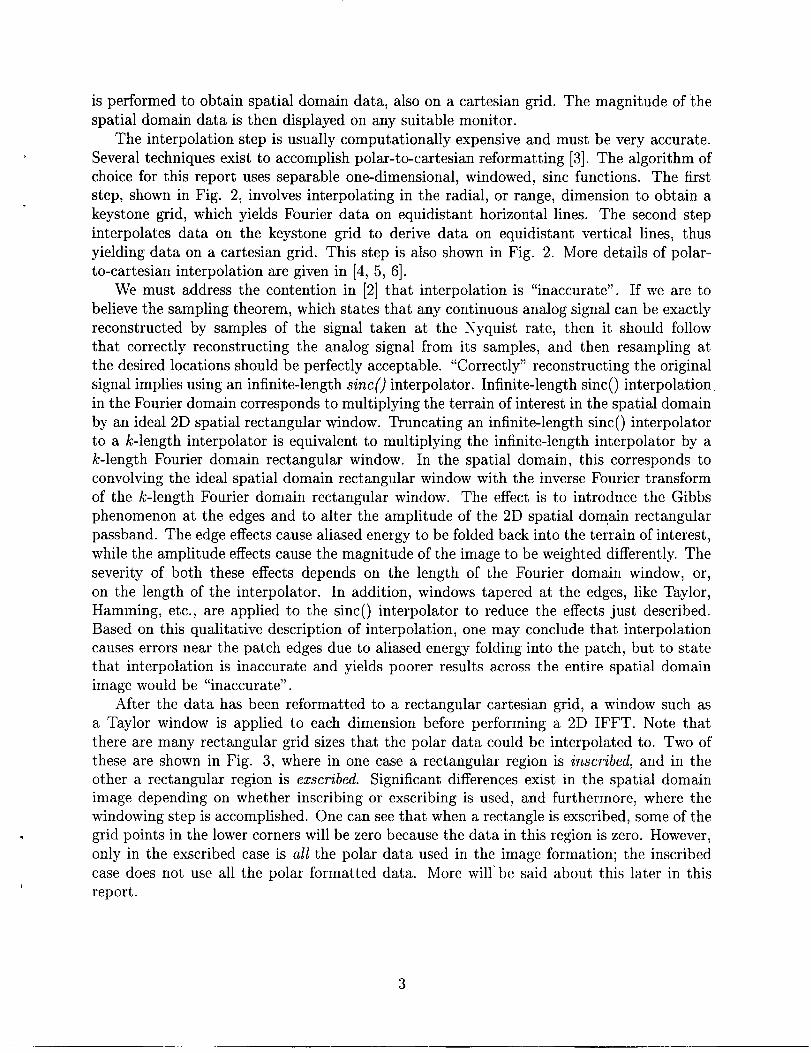
The interpolation step is usually computationally expensive and must be very accurate.Several techniques exist to accomplish polar-to-cartesian reformatting [3]. The algorithm ofchoice for this report uses separable one-dimensional, windowed, sine functions. The firststep, shown in Fig. 2, involves interpolating in the radial, or range, dimension to obtain akeystone grid, which yields Fourier data on equidistant horizontal lines. The second stepinterpolates data on the keystone grid to derive data on equidistant vertical lines, thusyielding data on a cartesian grid. This step is also shown in Fig. 2. More details of polar-to-cartesian interpolation are given in [4, 5, 6].

We must address the contention in [2] that interpolation is “inaccurate”. If we are tobelieve the sampling theorem, which states that any continuous analog signal can be exactlyreconstructed by samples of the signal taken at the Nyquist rate, then it should followthat correctly reconstructing the analog signal from its samples, and then resampling atthe desired locations should be perfectly acceptable. “Correctly” reconstructing the originalsignal implies using an infinite-length sinco interpolator. Infinite-length sinco interpolationin the Fourier domain corresponds to multiplying the terrain of interest in the spatial domainby an ideal 2D spatial rectangular window. Truncating an infinite-length sinco interpolatorto a k-length interpolator is equivalent to multiplying the infinite-length interpolator by ak-length Fourier domain rectangular window. In the spatial domain, this corresponds toconvolving the ideal spatial domain rectangular window with the inverse Fourier transformof the k-length Fourier domain rectangular window. The effect is to introduce the Gibbsphenomenon at the edges and to alter the amplitude of the 2D spatial domain rectangularpassband. The edge effects cause aliased energy to be folded back into the terrain of interest,while the amplitude effects cause the magnitude of the image to be weighted differently. Theseverity of both these effects depends on the length of the Fourier domain window, or,on the length of the interpolator. In addition, windows tapered at the edges, like Taylor,Hamming, etc., are applied to the sinco interpolator to reduce the effects just described.Based on this qualitative description of interpolation, one may conclude that interpolationcauses errors near the patch edges due to aliased energy folding into the patch, but to statethat interpolation is inaccurate and yields poorer results across the entire spatial domainimage would be “inaccurate”.

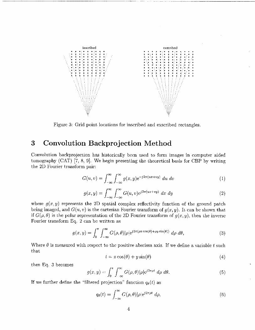
After the data has been reformatted to a rectangular cartesian grid, a window such asa Taylor window is applied to each dimension before performing a 2D IFFT. Note thatthere are many rectangular grid sizes that the polar data could be interpolated to. Two ofthese are shown in Fig. 3, where in one case a rectangular region is inscribed, and in theother a rectangular region is exscribed. Significant differences exist in the spatial domainimage depending on whether inscribing or exscribing is used, and furthermore, where thewindowing step is accomplished. One can see that when a rectangle is exscribed, some of thegrid points in the lower corners will be zero because the data in this region is zero. However,only in the exscribed case is all the polar data used in the image formation; the inscribedcase does not use all the polar formatted data. More will’ be said about this later in thisreport.

3

inscribed. . . . . *“.”””, “. . ‘.. :. ~.... .,

“.. i. :...:.; ..”.”“.. .’. .’....:. :. ..”.’* . ’. .:...:.:. .’. ”.’, .’. .:.0.: .: *.’..’. ’..’..’..:.’ .: .”.”,.,

“,“,‘.“,: ,’ ,’ .’ .’,. ..,...

exscribed. . . . . . . . . . . . . .“.. . . . “.. :.;.:.= . ..O* .’..*.’.. *.:....’. ..’. . ‘.. .“. .:. 0 . : .:.0’’..’ ●

.’. . “. ●: * :.*.:..’. .“. .”.

. “. .’. .:*:.*.: . .”..”..’.

. . ..”....:. . .: .:..’... .

. . . . .. .. .

. . ‘.. ‘.. “. “.

. . “.. .;“, “, “, :‘, ‘, ‘, :“, “, “, :“, ‘. ‘. “,‘, ‘, ‘, :‘. ‘. ‘. :‘. ‘, ‘. ‘,‘, ‘. “,:‘. ‘. “.:

. . . . . . . . .9.’.’ ..”0.. . .’ .’..

,’ ,’: .’ ,’ ,’: ,’ .’ .’: .“ .’ .“: ,“ ,“ ,“

,“ .“ ,’ ,“,“ ,“ ,“.“.“.“.“.’: ,’.’ .’,...,..,,.,

.. —..— :T

Figure 3: Grid point locations for inscribed and exscribed rectangles.

3 Convolution Backprojection Method

Convolution backprojection has historically been used to form images intomography (CAT) [7, 8, 9]. We begin presenting the theoretical basis forthe 2D Fourier transform pair:

G(u>V)

9(X, Y)

cow——

//9(~, ~)e

‘j2T(UZ+W/) du dv

—m —00

=/m/mG(u,v)e~2n(ux+w,)dz dy

computer aidedCBP by writing

(1)

(2)

where g (x, y) represents the 2D spatial complex reflectivity function of the ground patchbeing imaged, and G(u, v) is the cartesian Fourier transform of g(~, y). It can be shown thatif G (p, O) is the polar representation of the 2D Fourier transform of g (z, y), then the inverseFourier transform Eq. 2 can be written as

Where O is measured with respect to the positive abscissa axis. Ifthat

t = x cos(d) + y sin(d)

If we further define the “filtered projection” function go(t) as

dp dt?, (3)

we define a variable t such

(4)

(5)

(6)

4

.

.

then Eq. 5 becomes

/ ()9(~, y) = on qe t do. (7)

The two steps represented by Eqs. (6) and (7) define the CBP algorithm and allow a cartesianspatial domain image to be formed directly from polar Fourier domain data. Note that Eqs.(2) and (5) are essentially mathematical identities. That is,

The 2D function f(z, y) can be formed using either Eq. (2) or Eq. (5), but theoretically theresults should be identical!

Equation (6) represents the “convolution” portion of the CBP algorithm because qo(t) isnothing more than a linear filtering operation, i.e. a convolution. To see this, note that fora particular value of 0, the radial slice of the Fourier transform, G(p, 0), can be considereda one-dimensional function of p; call it PO(p). Equation (6) directs us to multiply Pe(p) by

[PI and then perform an inverse Fourier transform on the product. This is frequency domainfiltering. The equivalent time domain representation of Eq. (6) is

qe(~)= z%(~)* ~(~) (9)

where * denotes convolution,

w(t)= ~:wP)e’2”” dP

and

h(t) = ~w lpl#2”Pt dp. (11)—w

That is, h(t) is simply the impulse response of a filter whose frequency response is

H(p) = Ipl. (12)

After computing qe(t), this function must be “backprojected”, as specified by Eq. (7).The backprojection operation can be described by considering Eq. (7) together with Fig. 4,which shows a filtered projection for the angle 0. For every point on the cartesian grid, thevalue of t is computed, i.e.

tl = q COS(0)+ gl sin(0). (13)

The contribution to g(~l, VI) made by this projection function is q. (tl ) where -tI is givenby Eq. (13). Note that the point (xz, gz) will also give the same value of t, and thus thecontribution to g (Z2, g2) is also qe(tl ). In fact, for this value of O, every point on the linedefined by the two points (zl, yl) and (X2,y2) will receive the same contribution from q~(t). Inother words, all grid points lying on a line oriented at an angle 0 with respect to the horizontalaxis, and whose orthogonal distance to the origin is tl, will rekeive the same contribution from

qe(t), namely qe(tl).In this sense, the filtered projection is “backprojected” or “smeared”back onto the cartesian image. The integration of all filtered projections backprojected ontothe image yields the final result. Note that for only one angle do the points (ZI, yl ) and(X2,Vz) receive the same contribution.

5

% (t)

,, ...,,,, . ...’.,

,, ...,,,.,

..,,,,,, o(m,y,)

t 1;

. .. ... ... Yo” . 0 x,, . . .“’. . . . . . . . ,,,

Figure4: Image and filtered projection arrangement for backprojection step.

4 Modified CBP for SAR Image Formation

When considering data collected by a SAR, several medications are made to the fundamentalequations. Since data is nonzero only in the region shown in Fig. 1, the limits of integrationin Eq. (5) must be changed. Specifically, Eq. (5) becomes

One more simplification can be made by a simple change of variables:

With these steps, the filtered projection function is

and the backprojection equation becomes

/

~+Om9(~> Y) = qe(t)e~’mfctdtl.

;—@m

(14)

(15)

(17)

6

fc+$f

/ . . ., .,.,,.,

AZ-

2

H(p)

~

... .,,,. ,,, ,

c

fc_4y i

A$- P

2

Figure 5: Frequency domain specifications of filter for SAR data.

4.1 Discrete Implementation Issues

We begin discussing implementation issues by first considering the filtered projection Eq.(16). The change of variables performed in the previous paragraph shifted the Fourier datafrom a center frequency of fC to baseband. Thus, a one-dimensional FFT can be used toobtain qe(t) after the filtering operation. Note that due to the shift in frequency, the Fourierdata must be multiplied by a filter whose frequency characteristics match those shown inFig. 5 (i.e. a shifted segment of [pI).

Assuming that there are N. samples per pulse, the interval between samples in the radialdimension is

6,= :. (18)s

To use the FFT algorithm, the N, samples must be zero-padded to a length which is a powerof two. That is, we choose the FFT length to be Al, where 2~ > N$. As a result, the spacingbetween samples of qe(t) will be

N,&=&=-P MAf ‘

(19)

and therefore the values qe(ndt) will be available for use in the backprojection step. Notethat both positive and negative values of n are available.

Conversion of the backprojection step is straight forward. Since the angle subtended bythe radar is actually sampled, the backprojection formula Eq. (17) becomes

where 19zrepresents the angle of the it~ pulse, and NP is the number of pulses transmittedduring data collection. Normally there is a scale factor in front of the summation, butremoving it is inconsequential since all pixels are scaled by the same value.

During the backprojection step, the spacing between pixels in the spatial domain canbe arbitrarily assigned. For example, if dZ and 6V represent scale factors for the x and y

7

dimensions, respectively, then the value oft for some grid location (x, y) is computed using

t = xd. cos(f3) + @Ysin(~). (21)

One can see that if x and y are in units of “pixels”, and 6Z and 6V are in units of “dis-tance/pixel”, then the units of t will be distance. One may choose & and 6Yto “zoom in”or “zoom out” to any level desired.

Once the value oft is computed via Eq. (21), a decision must be made about what valueis backprojected to the point (x, g). One can easily see that it is likely t # ndt for all valuesof n. Therefore, one-dimensional interpolation must be performed to obtain the value qe(t),which is between q. (Mt ) and qe((ii * 1)&), where

h = integer value of (~), (22)

and + is used if t >0 and – is used if t <0.The one-dimensional interpolation step mentioned in the previous paragraph is a critical

issue. It is believed in [2] that linear interpolation or nearest neighbor assignment can beused to obtain qe(t). We believe that nearest neighbor assignment is not conducive to SARimage formation because this nonlinear operation would inject phase errors into the data.In addition, linear interpolation may be used but only if& <<1. Examples of the effects oflinear interpolation will be shown in a later section.

Multiplication by e~2Tfctin Eq. (20) is also a critical step. Unlike the 2DFFT method,where a shift of the data to the origin does not affect the magnitude of the spatial domainimage, the complex exponential in Eq. (20) is a function of@ and therefore must be includedin the integration over 0. Interpolation is not required to obtain the proper value of e~2~fCt;use the exact value for t from Eq. (21).

5 SAR Simulations

We have the benefit of using a spotlight mode synthetic target generator to simulate actualSAR data collections. All required parameters for SAR data collection can be specified;some of these include bandwidth, center frequency, chirp rate, pulse repetition frequency,collection geometry, and the number and location of as many targets desired. The simulatorprovides phase history data (i.e. Fourier domain data) as though it were a real SAR.

If there are differences in image quality depending on the formation technique used,we are more likely to see the variations if we have high resolution. For this reason, wemaintain the SAR parameters to provide one foot (0.3m) resolution in both range andazimuth (crom-range). We accomplish 0.3m resolution in range by using a pulse bandwidthof 500 MHz, which translates to A j = ~5x108 = 3.3333m–l. If VTrepresents the achievablerange resolution, then

1

The achievable azimuth resolution, -y., is approximately given by [1]

(23)

c‘Ya%—4fc9m ‘

(24)

8

Figure 6: Target arrangement on ground patch for simulations,

where Af, ~C,and On are shown in Fig, 1. We choose four sets of pairs (fC, 13n) to maintain

Y. x 0.3m. These are: A-(223 .3m-1, 0.42760), B-(lOOm-l, 0.95490), C-(50m-1, 1.91020),and D-(25m–1, 4.0000).

A standard arrangement of targets on the ground is used for each simulation. Thearrangement, shown in Fig. 6, encompasses all the extreme locations where a target maybe located, i.e. near range, patch center, far range, azimuth edge, and a combination of farrange - azimuth edge. It has been our experience that targets near the center of the patchbehave nicely under most circumstances, so we include targets at the patch edges.

We form the simulated images exactly like we form non-simulated images. This is animportant distinction from the work done in [2], where the grid size was chosen so thatthe nulls of the sidelobes fall on a grid point, thereby entirely removing sidelobes from theimage. Sidelobes are an important and unavoidable consequence of using finite length dataand therefore should be examined along with the mainlobe.

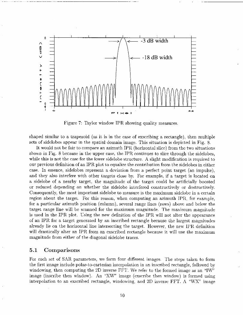
When we measure the quality of an image, we avoid using the multiplicative noise ratio[2] because it ignores sidelobe issues. Instead, we use three quality measures that we judge torepresent how closely a target resembles an impulse: -3 dB width, -18 dB width, and peak-to-sidelobe (PSL) ratio. To illustrate our use of these measures, refer to Fig. 7, which showsthe impulse response (IPR) of a Taylor window. The plots are always normalized so thatthe peak corresponds to O dB. Therefore, the PSL ratio can be measured by finding the levelof the highest sidelobe. In the example of Fig. 7, the IPR has the following characteristics:PSL ratio is -40 dB, -3 dB width is 1.25, -18 dB width is 2.8125.

A target’s IPR is measured by first extracting a slice of the image through the target,normally an azimuth (horizontal) slice or a range (vertical) slice. Then an FFT of the sliceis computed, the Fourier sequence is zero padded to a longer length, and an inverse FFT iscomputed, the magnitude of which is displayed. Zero padding to a longer length interpolatesbetween samples in the spatial domain and yields a smoother plot. The reason an azimuth orrange IPR is studied is because the sidelobes are usually in the azimuth and range dimension.This is because sidelobes extend in a direction orthogonal to the discontinuities in the Fourierdomain. For example, in the case of an inscribed rectangle, the Fourier domain edges are bothhorizontal and vertical, which gives rise to vertical and horizontal sidelobes, respectively, inthe spatial domain. On the other hand, if the nonzero region in the Fourier domain were

9

PTx-1——

Figure 7: Taylor window IPR showing quality measures.

shaped similar to a trapezoid (as it is in the case of exscribing a rectangle), then multiplesets of sidelobes appear in the spatial domain image. This situation is depicted in Fig. 8.

It would not be fair to compare an azimuth IPR (horizontal slice) from the two situationsshown in Fig. 8 because in the upper case, the IPR continues to slice through the sidelobes,while this is not the case for the lower sidelobe structure. A slight modification is required toour previous definition of an IPR plot to equalize the contribution from the sidelobes in eithercase. In essence, sidelobes represent a deviation from a perfect point target (an impulse),and they also interfere with other targets close by. For example, if a target is located ona sidelobe of a nearby target, the magnitude of the target could be artificially boostedor reduced depending on whether the sidelobe interfered constructively or destructively.Consequently, the most important sidelobe to measure is the maximum sidelobe in a certainregion about the target. For this reason, when computing an azimuth IPR, for example,for a particular azimuth position (column), several range lines (rows) above and below thetarget range line will be scanned for the maximum magnitude. The maximum magnitudeis used in the IPR plot. Using the new definition of the IPR will not alter the appearanceof an IPR for a target generated by an inscribed rectangle because the largest magnitudesalready lie on the horizontal line intersecting the target. However, the new IPR definitionwill drastically alter an IPR from an exscribed rectangle because it will use the maximummagnitude from either of the diagonal sidelobe traces.

5.1 Comparisons

For each set of SAR parameters, we form four different images. The steps taken to formthe first image include polar-to-cartesian interpolation in an inscribed rectangle, followed bywindowing, then computing the 2D inverse FFT. We refer to the formed image as an “IW”image (inscribe then window). An “XW’ image (exscribe then window) is formed usinginterpolation to an exscribed rectangle, windowing, and 2D inverse FFT. A “WX)’ image

10

Fourier domain shape spatial domain sidelobe structure

Figure8: Shows spatial domain sidelobe structure corresponding to Fourier domain shape.

(window then exscribe) is formed by first applying what amounts toa polar windowingscheme, then interpolate to an exscribed rectangle, followed by a 2D inverse FFT. Thefourth image is the “CBP” image formed using convolution backprojection. The windowsapplied were Taylor windows with -40 dB sidelobes.

We routinely use a 17-point sinco interpolator for polar-to-cartesian interpolation, whilein [2], the largest interpolator used was length 14. Judging from the results given in [2], a17-point interpolator would improve the MNR for the direct Fourier method in each case.

We focus most of our attention on the images formed using the “A” -image parameters,(fC, 13~) = (223.3m-’, 0.42760), and the “D’’-image parameters, (fC, 13~) = (25m-’, 4.000°)since these two represent the most extreme angle diversities. The ‘tA7’images are shown inFig. 9, while the “D” images are shown in Fig. 10. Note the sidelobes for each case fan outin a direction orthogonal to the discontinuities in the Fourier domain, as described earlier.Recall that the angle subtended in the “A” images is less than 1°; hence, the sidelobes appearsimilar to the inscribed case only because the angle between them is very small.

It is asserted in [2] that one reason CBP renders higher quality images is because all theFourier data are used. They refer to the fact that an inscribed rectangle does not use all theFourier data in the annulus shown in Fig. 1. This is what the authors of [2] must have meantwhen they stated that “polar-to-cartesian interpolation limits the achievable resolution, andtherefore, the final image quality.” This correlates well with our intuition and also withthe fundamental equations given in [1] showing that higher resolution is attainable if largerbandwidths are used. However, as pointed out previously, we are not restricted to interpolateto an inscribed rectangle. Furthermore, from a theoretical point of view, we can not forman image with better resolution than what the size of the collected Fourier data dictates.We can not magically create more Fourier data resulting in an improved image. We can,however, massage the data in different ways to better utilize the structure or format of thedata, as CBP appears to do by using the polar formatted data directly. Recall, however,that if the Fourier data is reformatted to an exscribed rectangular grid, or, if CBP is usedto form the image, all the Fourier data are used. Given the mathematics in Eq. (8), wehypothesized that similar quality images should result if the same steps are taken, in the

11

—

Figure 9: Images formed from “A” parameters. (a) IW. (b) XW. (c) CBP. (d) WX.(labeled clockwise from upper left)

12

. Figure 10: Images formed from “D” parameters. (a) IW. (b) XW. (c) CBP. (d) WX.(labeled clockwise from upper left)

13

same order, and the same Fourier data are used, regardless of the inverse Fourier transformtechnique, CBP or interpolation/2 DIFFT. This was the motivation for windowing the databe~ore reformatting to anexscribed rectangle. In fact, the windowing scheme employed inthe WX and CBP images are identical; the first step in either process is to window in therange (radial) dimension and then the cross-range (angular) dimension. If our hypothesis iscorrect, the difference between the WX and CBP images should be negligible.

Target IPR’s from each image formation technique using the “A” parameters are shownin Fig. 11, where the plots in Fig. 11(a) are from the center target and Fig. 11(b) arefrom the upper left target (azimuth edge-far range). Because the total angle subtended isonly 2& = 0.8552°, we do not expect much difference between the four image formationtechniques. The reason is because the Fourier data patch is nearly rectangular, and inscribinga rectangle does not discard large quantities of Fourier data. The results in Fig. 11 showthe following. First, the XW IPR exhibits the narrowest main lobe because the length of theTaylor window is longer in the cross-range dimension, and all the Fourier data are used. Itis well known that a longer window provides a narrower main lobe than a shorter window,and, Eq. (24) shows that if more bandwidth is used, better resolution results. While it isdifficult to see, the WX and CBP IPR’s are overlapping in the main lobe region and providethe second narrowest main lobe. It is true that both these techniques use all the Fourierdata, but the windows applied are only as wide as the actual data and therefore are shorter,resulting in a slightly wider main lobe than the XW case. The IW case yields the widestmain lobe because less Fourier data are used and the windows are shorter. The secondsignificant result is that while the PSL in the IW, WX, and CBP cases are nearly equal,the peak sidelobe in the XW case is considerably larger. This is due to the discontinuitiesin each of the lower corners of the Fourier domain patch. The quantitative values for theseIPR’s are given in Table 1. All these significant results should become more prominent asOn is increased.

Figures 12(a) and 12(b) show IPR’s from the center and upper left targets, respectively,generated using the “D” image parameters. The differences described in the preceding para-graph remain consistent for this case also, although they are more significant, as expected. Tosummarize, XW shows the narrowest main lobe but the largest PSL, IW exhibits the widestmain lobe, and WX and CBP are again overlapping in the main lobe and only slightly differ-ent in PSL’S. The differences are more pronounced in this case because the angle subtendedis now 20~ = 8°. Inscribing a rectangle discards a large amount of data, thus reducing thebandwidth considerably. Exscribing followed by windowing results in a large discontinuity inthe lower corners oriented at angles +0~ with respect to a vertical axis. It should be obviousthat as the angle subtended is increased, this effect is accentuated even more. Quantitativevalues for the “D” image targets are shown in Table 4.

Although we have examined IPR’s from only two targets from the “A” and “D” imagedata sets, these are representative of the entire data set. We have neglected to show rangeIPR’s because there was no significant difference between any of the images, regardless ofthe formation technique or SAR parameters.

Based on the preceding results, we conclude that the mathematical identity given in Eq.(8) is maintained in the case of SAR image formation. In retrospect, we should not expect theIW and XW images to produce the same images as WX and CBP for the simple reason thatdifferent steps are taken to obtain the final image. Conversely, if the same steps are followed,

14

.

>

.

0

nmuu

h+1-0[m+[

00

Figure 11:dash=XW,

(b)

“A” image (a) Center target IPR’s. (b) Upper left target IPR’s. Solid=IW,dot=WX, dot/dash=CBP.

15

nmuv

1-

0

[

0+[

nmuu

1-

Figure

0

00

0

00

(a)

12:

l= Txels

(b)

“D” image (a) Center target IPR’s. (b) Upper left target IPR’s. Solid=IW,dot=WX, dot/dash=CBP.

Table 1: IPR Measurements for “A” Image Data

IW Xw I Wx CBP

Center Target-3dB 1.8612 1.8362 1.8443 1.8417

-18dB 4.1581 4.0943 4.1204 4.1217PSL -40.0896 -38.4982 -39.5972 -40.1557

Upper Left Target-3dB 1.8625 1.8377 1.8421 1.8407

-18dB 4.1546 4.0897 4.1118 4.1213PSL -38.6378 -37.2457 -38.1568 -40.1561

Table 2: IPR Measurements for “B” Image Data

n IW Xw I Wx CBP 11

II Center Target II

I -3dB I 1.8500 \ 1.8011 ~ 1.8189 I 1.8081-18dB 4.1350 4.0067 4.0640 4.0450

PSL -40.0988 -37.3462 -39.6283 -40.2694

Urmer Left Tarszet-3dB I 1.8365-I’ 1.7893 I “1.8047 I 1.8081

-18dB 4.1088 3.9816 4.0356 4.0435PSL -38.2566 -35.8288 -37.7706 -40.2873

Table 3: IPR Measurements for “C” Ima~e Data

IW Xw Wx I “CBP

Center Target-3dB I 1.9452 I 1.8434 ~ 1.8799 I 1.8778

-18dB 4.3509 4.0842 4.2002 4.2026PSL -39.6552 -35.4441 -39.4776 -40.2289

Upper Left Target-3dB 1.9342 1.8348 1.8652 1.8780

-18dB 4.3305 4.0682 4.1768 4.2004PSL -38.3770 -34.3389 -37.7368 -40.0441

17

Table 4: IPR Measurements for “D” Image Data

Xw Wx CBP

Center Target-3dB 1.9145 1.7205 1.7886 1.7848

-18dB 4.2874 3.7863 3.9989 3.9954PSL -40,0168 -32.7780 -39.6069 -40.1483

~

Upper Left Target1.9111 1.7157 1.7790 1.80004.2750 3.7799 3.9860 4.0127

PSL -38.8986 -32.1347 -38.2308 -39.5324

i.e. window followed by inverse Fourier transform (either by CBP or interpolation/IFFT),then we should expect, based on Eq. (8), that the resultant images would be nearly identical.The only artifactual differences between the WX and CBP methods are due to numericalimplementation error, which are likely manifested in varying sidelobe levels because thesedifferences are extremely small.

Another visual illustration of the above conclusion is shown in Fig. 13, where two phasehistory domain images from the “D” parameter set are offered. The phase history domainimage is obtained from the spatial domain image via a 2D Fourier transform. Phase historyis a term used to specify the actual Fourier domain data collected by the SAR. Figure 13(a)shows the 2D Fourier transform (via FFT) of the WX image (Fig. 1O(C)), while Fig. 13(b)displays the 2D Fourier transform (via FFT) of the CBP image (Fig. 10(d)) . One cansee that the Fourier data used to form the CBP image (Fig. 13(b)) does in fact resemblethat which was obtained by first windowing and then interpolating to an exscribed rectangle(Fig. 13(a)). Note the angle of the edges in each phase history domain image correspondsto On = 4.0° with respect to a vertical axis.

5.2 One Dimensional Interpolation of Filtered Projections

In this section we revisit the issue of how to compute qg(t) if t # n& for any value of n. Thistopic was briefly addressed in [10] for nearest neighbor interpolation. We find that linearinterpolation can be used but only if dt << 1. To show the importance of this restriction, wepresent several examples, each using linear interpolation and having a different value for &.For the “D” parameter set, the SAR collects 381 pulses and samples each pulse 332 timesper second (N. = 332). To obtain the filtered projection function q.(t) given in Eq. (16),we perform the multiplication specified, zero pad the sequence to a length ill, and finishwith a length A4 inverse FFT to obtain samples of q.(t) at points separated by 6t given inEq. (19). Normally, one would chose ill = 512 if N. = 332, which gives & = 0.194531. Ifwe form a CBP image using ill = 512, and then extract from the image the center row,which contains the center and left targets, and plot the magnitude (normalized with respectto the maximum value), we obtain the plot shown in Fig. 14. If we let AZ = 1024 then& = 0.097266 and the same row extracted from the new image is shown in Fig. 15. Plotsin Figs. 16 and 17 result from M = 2048, & = 0.048633 and Al = 4096, & = 0.024316,respectively.

18

(a)

Figure 13: Phase history domain images from “D”

(b)

parameters. (a) WX. (b) CBP.

19

A

al

u

w

>

+

#

m

[

[

+

[

o

0N

ot

o0

0a

o0r

iNrI

I I I I I I I I I I I I I I I

0co 1 Umn

Figure 14: Center row from CBP

I I I I I I I I I I I I I I

511Num b-r

“D” image, N,=332, ik? =512.

0

Figure 15: Center

co I Umn

row from CBP

5 -I-INumb- r

“D” image, N,=332, Lf =1024,

0

co 1 umn511

Numb aI-

Figure 16: Center row from CBP “D” image, IV~=332, Al =2048.

A0

co I Umn

Figure 17: Center row from CBP

Number-..

.

“D” image, N. = 332, M = 4096,

21

All plots in Figs. 14 through 17 use the same scale to simplify comparison. Two veryimportant observations can be made from these plots. First, for the left target, one can seethat linear interpolation is inadequate for the larger values of & because additional targetshave begun to appear. These additional targets were first termed “false targets” in [11], butto our knowledge, the false targets were not mentioned again in any literature concerningCBP and SAR, nor was an explanation given for their existence. The second importantobservation from these plots is that the center target has not generated any false targets.Our results have shown that for a specific angle O~, as targets move further from the cross-range center, larger false targets are generated and the false target distance from the truetarget increases. Furthermore, as the angle 6~ becomes smaller, either by increasing fC anddecreasing 0~ to maintain resolution, or by decreasing em to reduce resolution, then theeflects shown in Figs. lJ through 17 become less severe.

To show this effect more dramatically, refer to the images in Fig. 18. We have strategicallyplaced targets in the ground patch so that the predominant position variation is either rangeor azimuth. The images in (a) and (b) were formed using the “D” image parameters, so theangle subtended by the radar is 20n = 8°. The only difference between these two images isthat Fig. 18(a) used M = 512 and Fig. 18(b) used M = 4096. Note in Fig. 18(a) that asa target’s azimuth position is increased from zero, the false targets become larger and morespread out. Note also that multiple false targets actually occur, but false targets furtherfrom the true target reduce in amplitude. Multiple false targets can also be seen in theone dimensional plots in Figs. 14 through 16. Finally, one can see in Fig. 18(b) that zeropadding to a longer length removes these effects. It should be pointed out that the act ofzero-padding to longer lengths essentially implements lD sinco interpolation!

While we can not offer theoretical guidelines for using linear interpolation, the conditionsoutlined in the previous paragraph, under which linear interpolation is not acceptable, dohave a common thread. Referring to Fig. 19, we see that a point target at location (xl, O)gives a projection function

q@(t) = d(t – tl) (25)

where tl = Z1 COS(0) and 60 is the unit sample function. If $ — 0~ < 0 < ~ + 19n, thenthe range of tl is –~1 sin(on) < tl < xl sin(~~). Thus, as Z1 becomes larger, the range ofvalues tl takes on also becomes larger as @progresses through it’s range. Similarly, as 0~ isincreased, the range of tl also increases for xl constant. It is apparently the large range ofvalues of tl, coupled with backprojecting a complex exponential (see Eq. (20)) onto a finitegrid that produces the false targets. The reason this effect was neither noted nor shown in[2] is most likely because their simulations used 20~=0.1875°.

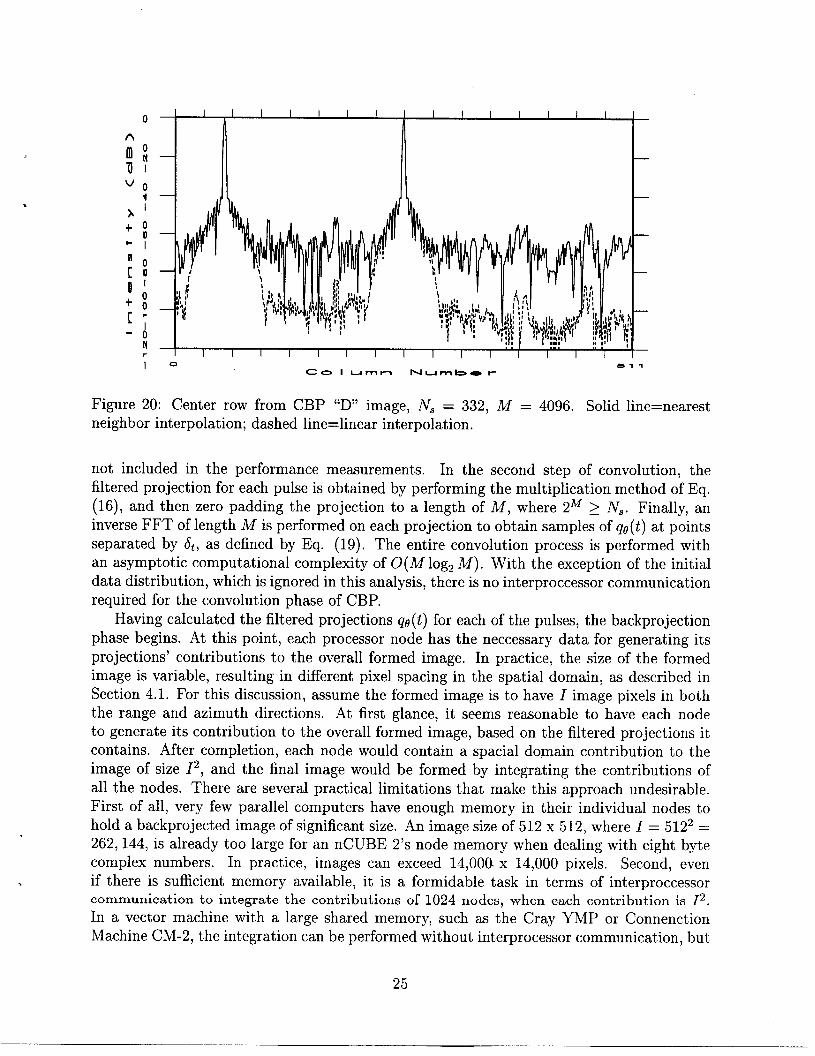
It is instructive to compare linear interpolation with nearest neighbor interpolation todetermine if the simpler interpolation scheme is adequate with the smaller value of &. Thiscomparison is shown in Fig. 20, where the center row from an image formed using nearestneighbor interpolation (solid graph) is compared with the same row using linear interpolation(dashed graph), with M = 4096, & = 0.024316. One can see that linear interpolation reducesthe noise floor by approximately 30dB or more. It is recommended that the additionalcomputations for linear interpolation be used to achieve this advantage.

22

(a) (b)

Figure 18: CBP-formed images(a) “D’’imagewithAf=5l2. (b) “D’’imagewithi M=4O96.

23

-Lt@(t)

,, ,, ,, ,, ,,,, ,,

tl,” “’’ ...,,,,,,,,,,,,,,,,, .

/ ‘-u’,,.xl, ,,, ,,

900 – ex,,

,, ,, ,, ,, ,, ,, ,,

Figure 19: Projection

6 Massively Parallel

function for image with single impulse.

Implementations

From a conceptual standpoint, the CBP algorithm is straightforward to parallelize. This wasmentioned in [2] as an advantage of the CBP algorithm over the 2DFFT method. However,from an implementation point of view, there are practical constraints that limit the perfor-mance of CBP when running on a parallel machine. Thus, the computation time required toform an image using CBP is significantly longer than with the 2DFFT method, while offeringno real simplification in the ease of parallelization. The parallel program described hereinwas designed for execution on a 1024-node nCUBE 2. Its execution times will be comparedto that of the 2DFFT algorithm on the same machine. While tests of CBP were not run onthe Connection Machine CM-2 and Cray Y-MP, references will be made to implementationissues on those architectures as well.

The convolution and backprojection portions of CBP are inherently independent and aretreated as two discrete phases in the parallel algorithm. The convolution portion of CBPis done in three steps. First, the complex phase history data are distributed as evenly aspossible among the computer’s p processors. The phase history pusles are distributed tothe processors along with their respective angle 0, as measured with respect to the positiveabscissa axis. When the total number of pulses, NP, is divided envenly by the numberof processors, p, then NP/p pulses are given to each node. If the division results in aremainder of r pulses, then the first r processors will receive an additional pulse to process.The data are read from either a singlepreviously striped across the disks. As

disk or a disk array, with thewith the 2DFFT method, disk

24

data having beentransfer times are

,

*

o I I I I I I I I I I I I I II I

A

m!111Uo

*

N1-

10 511Co I umm Numbet-

Figure 20: Center row from CBP “D” image, N, = 332, Ill = 4096. Solid line=nearestneighbor interpolation; dashed line= linear interpolation.

not included in the performance measurements. In the second step of convolution, thefiltered projection for each pulse is obtained by performing the multiplication method of Eq.(16), and then zero padding the projection to a length of M, where 2~ > N,. Finally, an—inverse FFT of length A4 is performed on each projection to obtain samples of qe(t) at pointsseparated by &, as defined by Eq. (19). The entire convolution process is performed withan asymptotic computational complexity of 0 (Al logz Ill). With the exception of the initialdata distribution, which is ignored in this analysis, there is no interproccessor communicationrequired for the convolution phase of CBP.

Having calculated the filtered projections qg(t) for each of the pulses, the backprojectionphase begins. At this point, each processor node has the necessary data for generating itsprojections’ contributions to the overall formed image. In practice, the size of the formedimage is variable, resulting in different pixel spacing in the spatial domain, as described inSection 4.1. For this discussion, assume the formed image is to have 1 image pixels in boththe range and azimuth directions. At first glance, it seems reasonable to have each nodeto generate its contribution to the overall formed image, based on the filtered projections itcontains. After completion, each node would contain a spatial domain contribution to theimage of size 12, and the final image would be formed by integrating the contributions ofall the nodes. There are several practical limitations that make this approach undesirable.First of all, very few parallel computers have enough memory in their individual nodes tohold a backprojected image of significant size. An image size of 512x 512, where 1 = 5122 =262,144, is already too large for an nCUBE 2’s node memory when dealing with eight bytecomplex numbers. In practice, images can exceed 14,000 x 14,000 pixels. Second, evenif there is sufficient memory available, it is a formidable task in terms of interproccessorcommunication to integrate the contributions of 1024 nodes, when each contribution ia 12.

In a vector machine with a large shared memory, such as the Cray YMP or ConnectionMachine CM-2, the integration can be performed without interprocessor communication, but

25

memory limitations would require repetitive swapping to and from disk of image portionsduring calculation.

To work more efficiently within the memory constraints of the parallel computer, considerthe following method of parallel backprojection. Instead of having each processor compute itscontribution to the overall space domain image, restrict the processor nodes to computingonly a portion of the formed image. For an image size of 12, where 1 is a power of 2,let the first processor compute the first I/p rows of the image, the second processor thenext I/p rows, etc. After each processor, in parallel, has integrated the contributions ofits filtered projections, they pass their filtered projections to another processor, and receivethose of another. This process continues until all nodes have received pulses from every otherprocessor, and have backprojected and integrated the contributions into their portion of thefinal image. This method minimizes the amount of memory required and results in a portionof the final image residing in each node, allowing for easy storage onto the disk or disk array.However, this method has the disadvantage of requiring 0 (p2) communication steps, unlessparallelism in communication is exploited.

To minimize communication steps within the nCUBE 2, the nodes are configured as anend-connected ring. After a node backprojects the filtered projections it contains, it sendsthem to the next higher processor, as numbered using a Gray coded ordering scheme. It thenreceives another set of filtered projections from its next lower node, as based on the Graycoding scheme. The backprojection is then performed on the new filtered projections withinthe node. In this way, all processors communicate with a hard-wired nearest neighbor, andthe entire ring-shift of data occurs within one communication step, since all nearest neighborcommunication takes place simultaneously. By the end of only O(p) communication steps,all filtered projections have been seen by all processor nodes. Each processor requires 0(1)calculations to backproject each filtered projection, resulting in an overall complexity ofO(lV~), when the input phase history is similar in size to the formed space domain image.The communication time required to shift the filtered projections one position in the ring isa linear function of the length of the filtered projection, namely IM. When significant zeropadding of the input pulse is required, Al increases and communication time suffers. Thisis a potential disadvantage of CPB over the 2DFFT method, since 2DFFT doesn’t requirepadding beyond rounding to the next higher power of 2.

Regardless of the parallel method used to implement the CBP algorithm, it’s likely to beless efficient that the 2DFFT method. This is due to CBP’S ‘expansion’ of data, whereby asmaller filtered projection is backprojected onto a larger space domain image. This resultsin an increased amount of communication, since the space domain contributions within thenodes must be integrated into a single formed image through a data gathering operation.When a node does not backproject over the entire space domain, but instead, is responsiblefor the formation of a portion of the image, memory is conserved. However, the node musthave access to all filtered projections within all other nodes. Either way, a considerableamount of interprocessor communication is required. While the CBP method requires O(p)communication steps, the bulk of communication in the 2DFFT method is due to the matrixtransposition, which takes only O(logzp) steps.

Table 5 contains actual running times for the CBP and 2DFFT algorithms on a 1024 nodenCUBE 2. The running time of both algorithms increases proportionally with the squareof the input data size. However, due to the data expansion in the CBP algorithm and the

26

,

Table 5: Running Time (see) for CBP and 2DFFT on a 1024 Node nCUBE2

UPh. Hist. Size II CBP II 2DFFT I

m

associated increase in communication cost, the constant multiplier for the CBP algorithm ishigher. Data transfers to and from disk were not considered in these timings.

7 Conclusions

It should be evident that resolution and, therefore image quality, is dependent on the sizeof the Fourier data patch obtained during aperture synthesis, and not so dependent on theimage formation technique used. In the case of inscribing a rectangle in the polar annulus,Fourier data is discarded, which reduces the achievable resolution. When the polar data isinterpolated to an exscribed rectangle followed by windowing, the tapered window extendsto the edges of the rectangular region, leaving a sizable discontinuity beginning in the uppercorners, oriented at an angle corresponding to the collection geometry. While the main lobesof point targets are narrower, the sidelobes are much larger because of the discontinuity.This results in a poorer quality image.

If the entire Fourier data are windowed, followed by 2D Fourier inversion without dis-carding any data, then mathematics and experimental results show that regardless of theFourier inversion technique, the image quality will be identical, save for insignificant nu-merical artifacts. This was the case for convolution backprojection and interpolating to anexscribed rectangle followed by 2D IFFT. The two methods appear to offer the best resultsin terms of the tradeoff between narrower mainlobe and very low sidelobes. However, somemay argue that the more complex sidelobe structure detracts from the appearance of theimage. For broadside mode collection, inscribing a rectangle generates sidelobes in only 4directions, but the other methods force the user to contend with sidelobes in 6 directions.

Note that if the polar data is first interpolated to an exscribed rectangle, and then aprogressively tapered window is applied so that the ends of the window correspond to thediscontinuity, then results similar to CBP and WX are obtained. In this case, however,applying the window is much more complicated than in any of the other cases because thewindow length for each row must be computed and a new window generated.

The CBP algorithm is straightforward to parallelize. However, several practical con-straints limit the efficiency of the computations. The zero padding of pulses during theconvolution phase results in longer messages, thereby increasing communication time. Fur-thermore, an expansion of data results from the backprojection of individual filtered pro-jections onto a larger space domain. This drives up memory requirements and results inincreased communication overhead, since each node’s contribution to the space domain im-age must be globally integrated. Alternatively, each node can be made responsible for theformation of a portion of the final image. This reduces memory requirements and eliminates

27

the global gathering operation. Unfortunately, this approach requires each node to haveaccess to all other nodes’ projections, thereby increasing communication time. The CBPalgorithm does allow for the variable scaling of the formed image., which isn’t a feature ofthe 2DFFT. However, the computation times of the CBP method are significantly longerthan those of the CBP method, and as the size of the input data set increases, the CBPmethod falls farther behind the 2DFFT in efficiency.

28

References

[1]

[2]

[3]

[4]

[5]

[6]

[7]

[8]

[9]

[10]

[11]

D. C. Munson, J. D. O’Brien, and W. K. Jenkins, “A tomographic formulation ofspotlight-mode synthetic aperture radar,” Proceedings of-the L?L?L?3,pp. 917–925, August1983.

M. D. Desai and W. K. Jenkins, “Convolution backprojection image reconstruction forspotlight mode synthetic aperture radar,” IEEE Trans. on Image Processing, pp. 505-517, October 1992.

D. C. Munson, J. L. C. Sanz, W. K. Jenkins, G. Kakazu, and B. C. Mather, “A com-parison of algorithms for polar-to-cartesian interpolation in spotlight mode sar,” Proc.Int. Conf. on Acoustics, Speech, and Signal Processing, pp. 1364-1367, March 1985.

G. A. Mastin and D. C. Ghilia, “A research-oriented spotlight synthetic aperture radarpolar reformatter,” Tech. Rep. SAND90-1793, Sandia National Laboratories, Reprinted

October 1993.

G. A. Mastin and D. C. Ghilia, “An enhanced spotlight synthetic aperture radar po-lar reformatter,” Tech. Rep. SAND91-0718, Sandia National Laboratories, ReprintedOctober 1993.

G. A. Mastin, S. J. Plimpton, and D. C. Ghilia, “A massively parallel digital processorfor spotlight synthetic aperture radar,” The International Journal of SupercomputerApplications, vol. 7, pp. 97-112, Summer 1993.

G. T. Herman, image Reconstruction from Projections. Academic Press, 1980.

A. Rosenfeld and A. C. Kak, Digital Picture Processing. Academic Press, 1982.

E. S. Haykin, Array Signal Processing. Prentice-Hall, 1985.

M. D. Desai, A New Method of Synthetic Aperture Radar Image Reconstruction UsingModified Convolution Backprojection algorithm. PhD thesis, Univ. of Illinois, 1985.

M. D. Desai and W. K. Jenkins, “Convolution backprojection image reconstruction forsynthetic aperture radar,” Proceedings of ISCAS, pp. 261-263, 1984.

This work was supported by the U.S. Department of Energy under contract DE-AC04-76DPO0789.

29

Distribution

1

1

1

21113112

1

52

3

Dr. Gregory DonohoeEECE DepartmentUniversity of New MexicoAlbuquerque, NM 87131

Dr. Don HushEECE DepartmentUniversity of New MexicoAlbuquerque, NM 87131

Dr. Neeraj MagotraEECE DepartmentUniversity of New MexicoAlbuquerque, NM 87131

MS 0572 C.V. Jakowatz, 5912

0572 D.E. Wahl, 59120572 P.A. Thompson, 59120572 T.J. Flynn, 59120572 N.E. Doren, 59120978 L.G. Stotts, 59341110 D.C. Ghiglia, 92231436 C. Meyers, 4523

9018 Central Technical Files, 8523-20899 Technical Library, 44140619 Review and Approval Desk, 12630

For DOE/OSTI0161 Patent and Licensing Office, 11500

30