Estimates of marine mammal, turtle, and seabird mortality for two ...

ARTICLE IN PRESS
0967-0645/$ - see
doi:10.1016/j.ds
�CorrespondiE-mail addre
Deep-Sea Research II 53 (2006) 741–770
www.elsevier.com/locate/dsr2
A comparison of global estimates of marine primary productionfrom ocean color
Mary-Elena Carra,�, Marjorie A.M. Friedrichsb,bb, Marjorie Schmeltza,Maki Noguchi Aitac, David Antoined, Kevin R. Arrigoe, Ichio Asanumaf,Olivier Aumontg, Richard Barberh, Michael Behrenfeldi, Robert Bidigarej,
Erik T. Buitenhuisk, Janet Campbelll, Aurea Ciottim, Heidi Dierssenn,Mark Dowello, John Dunnep, Wayne Esaiasq, Bernard Gentilid, Watson Greggq,
Steve Groomr, Nicolas Hoepffnero, Joji Ishizakas, Takahiko Kamedat,Corinne Le Querek,u, Steven Lohrenzv, John Marraw, Frederic Melino,
Keith Moorex, Andre Moreld, Tasha E. Reddye, John Ryany, Michele Scardiz,Tim Smythr, Kevin Turpieq, Gavin Tilstoner, Kirk Watersaa, Yasuhiro Yamanakac
aJet Propulsion Laboratory, California Institute of Technology, 4800 Oak Grove Dr, Pasadena, CA 91101-8099, USAbCenter for Coastal Physical Oceanography, Old Dominion University, Crittenton Hall, 768 West 52nd Street, Norfolk, VA 23529, USAcEcosystem Change Research Program, Frontier Research Center for Global Change, 3173-25,Showa-machi, Yokohama 236-0001, Japan
dLaboratoire d’Oceanographie de Villefranche, 06238, Villefranche sur Mer, FranceeDepartment of Geophysics, Stanford University, Stanford, CA 94305-2215, USA
fTokyo University of Information Sciences 1200-1, Yato, Wakaba, Chiba 265-8501, JapangLaboratoire d’Oceanographie Dynamique et de Climatologie, Univ Paris 06, MNHN, IRD,CNRS, Paris F-75252 05, France
hDuke University Marine Lab, 135 Duke Marine Lab Rd, Beaufort, NC 28516, USAiDepartment of Botany and Plant Pathology, Cordley Hall 2082, Oregon State University, Corvallis, OR 97331, USA
jDepartment of Oceanography, University of Hawaii, Honolulu, HI 96822, USAkMax-Planck-Institute for Biogeochemistry, Postfach 100164, D07701 Jena, Germany
lMorse Hall, University of New Hampshire, 39 College Road, Durham, NH 03824-3525, USAmUNESP - Campus do Litoral Paulista, Prac-a Infante Dom Henrique S/N, Sao Vicente, Sao Paulo CEP 11330-900, Brazil
nDepartment of Marine Sciences, University of Connecticut, 1080 Shennecossett Road, Groton, CT 06340, USAoJoint Research Center of the E.C., Inland and Marine Waters Unit I-21020, Ispra (Va), Italy
pNOAA/Geophysical Fluid Dynamics Laboratory, PO Box 308, Forrestal Campus B Site, Princeton, NJ 08542-0308, USAqNASA Goddard Space Flight Center, Global Modeling and Assimilation Office, Greenbelt, MD 20771, USA
rRemote Sensing Group, Plymouth Marine Laboratory, Prospect Place, Plymouth, Devon PL1 3DH, UKsFaculty of Fisheries, Nagasaki University, 1-14 Bunkyo, Nagasaki 852-8521, Japan
tGroup of Oceanography, National Research Institute of Far Seas Fisheries, 5-7-1 Shimizu-Orido, Shizuoka 424-8633, JapanuUniversity of East Anglia and the British Antarctic Survey, Norwich NR4 7TJ, UK
vDepartment of Marine Science, 1020 Balch Blvd., Stennis SpaceCenter, MS 39529-9904, USAwLamont-Doherty Earth Observatory, 61 Route 9W, Palisades, NY 10964, USA
xEarth System Science, University of California at Irvine, 3214 Croul Hall, Irvine, CA 92697-3100, USAyMBARI, 7700 Sandholdt Rd., Moss Landing, CA 95039-9644, USA
front matter r 2006 Elsevier Ltd. All rights reserved.
r2.2006.01.028
ng author. Tel.: +1818 354 5097; fax: +1 818 393 6720.
ss: [email protected] (M.-E. Carr).
ARTICLE IN PRESSM.-E. Carr et al. / Deep-Sea Research II 53 (2006) 741–770742
zDepartment of Biology, University of Rome ‘Tor Vergata’, Via della Ricerca Scientifica, 00133 Roma, ItalyaaNOAA Coastal Services Center, 2234 South Hobson Avenue Charleston, SC 29405-2413, USA
bbVirginia Institute of Marine Science, College of William and Mary, P.O. Box 1346, Gloucester Point, VA 23062, USA
Received 2 September 2004; accepted 30 January 2006
Abstract
The third primary production algorithm round robin (PPARR3) compares output from 24 models that estimate depth-
integrated primary production from satellite measurements of ocean color, as well as seven general circulation models
(GCMs) coupled with ecosystem or biogeochemical models. Here we compare the global primary production fields
corresponding to eight months of 1998 and 1999 as estimated from common input fields of photosynthetically-available
radiation (PAR), sea-surface temperature (SST), mixed-layer depth, and chlorophyll concentration. We also quantify the
sensitivity of the ocean-color-based models to perturbations in their input variables. The pair-wise correlation between
ocean-color models was used to cluster them into groups or related output, which reflect the regions and environmental
conditions under which they respond differently. The groups do not follow model complexity with regards to wavelength or
depth dependence, though they are related to the manner in which temperature is used to parameterize photosynthesis.
Global average PP varies by a factor of two between models. The models diverged the most for the Southern Ocean, SST
under 10 �C, and chlorophyll concentration exceeding 1mgChlm�3. Based on the conditions under which the model results
diverge most, we conclude that current ocean-color-based models are challenged by high-nutrient low-chlorophyll
conditions, and extreme temperatures or chlorophyll concentrations. The GCM-based models predict comparable primary
production to those based on ocean color: they estimate higher values in the Southern Ocean, at low SST, and in the
equatorial band, while they estimate lower values in eutrophic regions (probably because the area of high chlorophyll
concentrations is smaller in the GCMs). Further progress in primary production modeling requires improved understanding
of the effect of temperature on photosynthesis and better parameterization of the maximum photosynthetic rate.
r 2006 Elsevier Ltd. All rights reserved.
1. Introduction
Although photosynthesis is a key component ofthe global carbon cycle, its spatial and temporalvariability is poorly constrained observationally.Furthermore it is unclear how this variability mayrespond to potential scenarios of climate change.Global net primary production, the carbon fixedthrough photosynthesis and available for highertrophic levels, occurs in both terrestrial (52%) andmarine ecosystems (48%) (Field et al., 1998). Thehighly dynamic nature of marine photosynthesis isrevealed by considering that the annual mean valueof 45–50Gt C is carried out by a phytoplanktonbiomass of �1Gt. Ship resources cannot resolvelow-frequency spatial and temporal variability,much less make direct observations of mesoscalevariability beyond isolated snapshots. The chronicundersampling of ship-based estimates of globalprimary production requires significant extrapola-tions, making it essentially impossible to quantifybasin-scale variability from in situ measurements.
Fortunately, satellites provide a solution (McClainet al., 1998). Sensors that measure ocean color are
presently used to estimate chlorophyll concentrationin the upper ocean. Integrated biomass can beobtained from ocean color by assuming a verticalprofile and a carbon to chlorophyll relationship. Togo from biomass, a pool, to photosynthesis, a rate, atime dependent variable is needed. Solar radiation isan obvious choice, and simple mechanistic modelscompute productivity from biomass, photosyntheti-cally available radiation (PAR), and a transfer oryield function which incorporates the physiologicalresponse of the measured chlorophyll to light,nutrients, temperature, and other environmentalvariables. As a variable amenable to remote sensing,sea-surface temperature (SST) is often used toparameterize the photosynthetic potential.
There exist a range of modeling approaches, e.g.,Platt and Sathyendranath (1993), Longhurst et al.(1995), Howard and Yoder (1997), Antoine andMorel (1996), Behrenfeld and Falkowski (1997a), orOndrusek et al. (2001). These models can bedistinguished by the degree of explicit resolution indepth and irradiance as described by Behrenfeld andFalkowski (1997b). While vertically and spectrallyexplicit models incorporate information about algal
ARTICLE IN PRESS
Table 1
Model participants, type of model used, group to which they
belong, and parts of PPARR3 for which we have received results
No. Participants Type Group Parts
1 Carr WIDI 1 1, 2, 3
2 Behrenfeld WIDI 2 1, 2, 3
3 Behrenfeld WIDI 4 1, 2, 3
4 Turpie and Esaias WIDI 2 1, 2, 3
5 Ciotti WIDI 2 1, 2, 3
6 Ishizaka and Kameda WIDI 2 1, 2, 3
7 Moore WIDI 1 1
8 Dierssen WIDI 1 1, 2
9 Dierssen WIDI 1 1, 2
10 Dowell WIDI 2 1, 3
11 Turpie and Esaias WIDI 4 1, 2, 3
12 Ryan WIDI 3 1, 2, 3
13 Carr WIDI 4 1, 2, 3
14 Scardi WIDI 1 1, 2, 3
15 Lohrenz WIDR 2 1
16 Lohrenz WIDR 2 1
17 Lohrenz WIDR 3 1
18 Asanuma WIDR 3 1, 2, 3
19 Marra WIDR 4 1, 2, 3
20 Antoine, Gentili, and Morel WRDR 4 1, 2, 3
21 Smyth WRDR 4 1, 2, 3
22 Melin and Hoepffner WRDR 1 1, 2, 3
23 Waters and Bidigare WRDR 2 1, 2, 3
24 Arrigo and Reddy WRDR 4 1, 2, 3
25 Aumont GCM 5 1, 3
26 Moore GCM 5 1
27 Yamanaka and Aita GCM 5 1
28 Dunne GCM 5 1
29 Buitenhuis and Le Quere GCM 5 1, 3
30 Gregg GCM 5 1
31 Gregg GCM 5 1
See text for model and group description.
M.-E. Carr et al. / Deep-Sea Research II 53 (2006) 741–770 743
physiology and its dependence on environmentalfactors, the paucity of measurements of physiologi-cal characteristics on the global scale hinders theirfull application. A common parameter in manysimpler models is the maximum observed photo-synthetic rate (normalized by biomass) within thewater column (PB
opt). Another parameter, PBmax, is
derived from short-term light-saturated incubations;consequently extant measurements are fewer. PB
max
is defined as the maximum rate of photosynthesiswhen light is not limiting, while PB
opt represents theeffective photoadaptive yield in the field for specificlight conditions.
A series of round-robin experiments have beencarried out to evaluate and compare models whichestimate primary productivity from ocean color(Campbell et al., 2002). In these experiments, in situmeasurements of carbon uptake were used to testthe ability of the participating models to predictdepth-integrated primary production (PP) based oninformation accessible via remote sensing. The firstround-robin experiment used data from only 25stations. The second primary production algorithmround robin (PPARR2) used data from 89 stationswith wide geographic coverage (Campbell et al.,2002). There were 10 participant teams and 12models.
Eight models were within a factor of 2.4 (basedon one standard deviation in log-difference errors)of the 14C measurements (Campbell et al., 2002).Biases were a significant source of error. If biaseswere eliminated, 10 of the 12 model estimates wouldbe within a factor of two of the in situ data. Thealgorithms performed best in the Atlantic region,which has historically contributed the most data forparameterization. The equatorial Pacific and theSouthern Oceans presented the worst results. TheSouthern Ocean data included both the lowest andhighest values of primary production, so the poorperformance may be related to this dynamic range.The high-nutrient low-chlorophyll (HNLC) condi-tions observed in both the equatorial Pacific and theSouthern Oceans may contribute to the highermodel-data misfit, as most models were not devel-oped with data subject to micronutrient limitation.Likewise, globally-tuned parameterizations of tem-perature and of the vertical extent of surfacebiomass are likely to fail in both regions.
The third primary production algorithm roundrobin (PPARR3) compares output from 24 ocean-color-based models and model variants from theUS, Europe, Japan, and Brazil (Table 1). The first
part of PPARR3 is a comparison of monthly globalprimary production fields generated by the differentalgorithms while part 2 is a sensitivity analysis.These two parts do not use in situ data to quantifymodel performance. Therefore, it is not possible todefine a ‘best’ model. Part 3 is a ground-truthcomparison like PPARR1 and PPARR2. Wecompare modeled PP and a high quality databaseof 14C measurements from the tropical Pacific(Le Borgne et al., 2002). The poor performance ofthe PPARR2 models in the tropical Pacific and theplentiful high-quality data led us to emphasize thisregion within PPARR3. An upcoming manuscript(Friedrichs et al., in prep) will present the results ofpart 3 of PPARR3 and recommend the bestperforming model for the tropical database com-parison. A future study will look at a broader rangeof in situ data.
ARTICLE IN PRESSM.-E. Carr et al. / Deep-Sea Research II 53 (2006) 741–770744
Circulation and nutrient fields are necessary tofully quantify oceanic carbon fluxes and biologicalproductivity. In an effort to bring the ocean-color-based productivity modelers together with ecosys-tem and biogeochemical modelers, we invited thelatter group to participate so we can compare theirmodeled primary production fields for the sametime period with those of the ocean-color models.Our sole criterion for participation were that themodels simulate global primary production fields.
In this paper, we describe PPARR3 results fromparts 1 and 2, i.e. a global intercomparison ofmodels for eight months and a sensitivity analysis.Although a comparison with in situ data is neededto quantify the performance of the models, theintercomparison enables us to discern the conditionsunder which the models have divergent results. Bycomparing the model output, we can distinguishgroups, which in turn can be understood on thebasis of the sensitivity analysis. Here we address theobserved spatial, seasonal, and interannual varia-bility among the participating models.
2. Data and methods
2.1. Participating models
The participating models are of all types dis-cussed by Behrenfeld and Falkowski (1997b):wavelength- and depth-integrated (WIDI, 14 mod-els), wavelength-integrated and depth-resolved(WIDR, five models), and wavelength- and depth-resolved (WRDR, five models). The list of models isgiven in Table 1, classified by model type, with thename of the participant(s), and the PPARR3 partsto which they have contributed. Seven generalcirculation models coupled to biogeochemistry(GCM-based) have participated in part 1 (globaland regional intercomparison). The models aredescribed in the Appendix.
2.2. Approach
The input data required for the participants toestimate integrated primary production were pro-vided by the PPARR3 organizers Carr and Frie-drichs; the participants then returned their resultsfor subsequent comparison. In part 1, the inputfields corresponded to eight monthly mean globalmaps of chlorophyll from SeaWiFS, SST fromAVHRR Pathfinder, photosynthetically availableradiation (PAR) from SeaWiFS, and mixed-layer
depth estimated from two different general circula-tion models: the JPL-MIT model and the NCARmodel. Despite differences in the two fields ofmixed-layer depth, the impact on the resulting PPfields was almost negligible. Hereafter, we onlyshow results which used mixed-layer depth from theJPL-MIT model. The monthly means correspond toJanuary, March, May, July, September, November,and December 1998, and December 1999. Weworked at a nominal 18-km resolution obtainedby subsampling the 9-km standard-mapped-imagefields. The participants (Table 1) used these inputfields to estimate primary production integrated tothe 1% light level (hereafter PP). Here we comparethe resulting PP fields. The approach is outlined inFig. 1 for December 1998. This study does notprovide an estimate of the global PP for the studyperiod, but rather compares model output toidentify the conditions under which models diverge.In fact we have used Version 2 of SeaWiFS data(first reprocessing), but for our purpose of modelintercomparison, improved chlorophyll determina-tion has little bearing except in localized areas. Savetwo exceptions, the GCM-based models did not useany of the input variables that were so fundamentalto the ocean-color-based models. Participation ofthe GCM modelers was added after the projectdesign was developed. Model #26 used the MLDfields and model #31 assimilated the SeaWiFSchlorophyll, although not the same version andresolution as shown here.
The pair-wise linear correlation of the spatial andseasonal variability of the models enables us todistinguish four groups of ocean-color-based mod-els, within which the models are highly correlated,and among which the correlation is less (see Section3.1 below). To derive a mean model, we averagedthe models within each group together (omittingmodel #4 because it is identical to model #2) andthen averaged the four group-average modelstogether. The model spread is then quantified bycomparing each model with the mean model. Wecalculated the difference between the decimallogarithm (log base 10) of each model and that ofthe mean, which is in effect the logarithm of theratio between the model and the average model,following Campbell et al. (2002). We divided theglobal fields into basins, SST levels, chlorophyllconcentrations, and basin-latitudinal bands toevaluate model similarity and divergence. There isno reason to assume that the mean model is closerto truth than the outlier models that appear as

ARTICLE IN PRESS
MLDJ
m0 50 100 150 200
MLDN
m0 50 100 150 200
PAR
einstein m-2 d-10 15 30 45 60
SST
oC-1 9 19 29
Chl
mg m-30.01 0.1 1
MEAN MODELED PP
g C m-2 day-10.1 0.32 1 3.2
RANGE OF MODELED PP
g C m-2 day-10.1 0.32 1 3.2
Fig. 1. Approach taken in Part 1 of PPARR3. The ocean-color modelers were given monthly mean input files: mixed-layer depth from two
GCMs (MLDJ and MLDN), SST, PAR, and chlorophyll concentration. They estimated integrated primary production and returned their
values to the organizers. These are the input fields corresponding to January 1998 and the resulting ocean-color-mean model and the
observed range of ocean-color model estimates.
M.-E. Carr et al. / Deep-Sea Research II 53 (2006) 741–770 745
anomalous. However, the mean model provides astandard of consistency. If an anomalous model iscloser to ‘truth’ (which can be evaluated in part 3and in future ground-truth comparisons), its diver-gence from the mean model indicates that amajority of the models are far from truth.
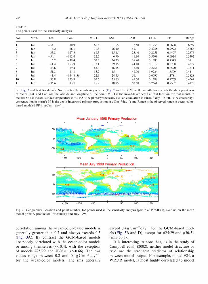
In part 2 of the PPARR3 exercise, the sensitivityof the models to the input variables was examinedby distributing data for 11 representative points, fivefrom January 1998 and six from July 1998 (Table 2and Fig. 2). These points correspond to a pixel(�18 km) and are chosen as representative ofseasonal and geographic variability, as well ascovering a range of input values and modelresponse. We then systematically varied the valueof each input variable, holding the others constant.The range of values for the input variables isroughly the range observed for our study period: forSST, �1 to 30 �C; for mixed-layer depth, 10–480m;for PAR, 5–60Einm�2 day�1; and for chlorophyllconcentration, 0.01–10mgm�3. The final databaseconsists of 385 values corresponding to the originaldata point and 34 variations at each geographicallocation. Carr and Friedrichs distributed thesevalues to the participants who then estimated PP,
from which we estimated the difference in thedecimal logarithm of PP for each perturbation ofthe input variable.
3. Results
3.1. Relationships among models
In PPARR2, production estimated from ocean-color algorithms was found to be highly correlatedand the correlation was independent of modelcomplexity (Campbell et al., 2002). In an attemptto group the models on the basis of related output,here we estimated pair-wise correlation and root-
mean-square (rms ¼ffiffiffiffiffiffiffiffiffiffiffiffiffiffiffiffiffiffiffiffiffiffiffiffiffiffiffiffiffiffiffiffiffiffiffiffiffiffiffiffiffiffiffiffiffiffiffiffiPðmodeli �model2j Þ=n
q) cor-
responding to the monthly global PP fields inJanuary and July 1998 (Fig. 3). The correlationcoefficient and rms between any pair of models isgenerally inversely related, with higher correlationbetween models with low rms (Figs. 3A and B). Thisis reassuring but not necessarily expected: correla-tion quantifies similarity in the variability while rmsis a measure of mismatch. Perfectly coincidentpatterns may present a large systematic bias. The
ARTICLE IN PRESS
Mean January 1998 Primary Production
23
4
5
11
-150 -100 -50 0 50 100 150
-50
0
50
Mean July 1998 Primary Production
1
6
7
8
9
10
-150 -100 -50 0 50 100 150
-50
0
50
Fig. 2. Geographical location and point number, for points used in the sensitivity analysis (part 2 of PPARR3), overlaid on the mean
model primary production for January and July 1998.
Table 2
The points used for the sensitivity analysis
No. Mon. Lat. Lon. MLD SST PAR CHL PP Range
1 Jul �54.1 30.9 66.6 1.65 3.60 0.1758 0.0628 0.6697
2 Jan 16.2 66.1 71.8 26.40 42. 0.4955 0.9922 0.4366
3 Jan 33.8 �127.3 68.3 15.15 23.40 0.2951 0.4497 0.2876
4 Jan �54.1 �162.4 32.5 6.90 41.10 0.5309 0.6914 0.3302
5 Jan 16.2 �39.4 70.3 24.75 38.40 0.1380 0.4543 0.39
6 Jul �1.4 153.9 37.1 29.85 44.10 0.1012 0.3708 0.4279
7 Jul �36.6 �39.4 63.0 16.05 15.60 0.2754 0.3570 0.3311
8 Jul 51.3 �21.8 15.7 15. 42.90 1.9724 1.8509 0.44
9 Jul �1.4 �144.8436 22.9 24.45 51. 0.6095 1.1781 0.3828
10 Jul 33.8 153.9 10.7 25.05 49.50 0.1288 0.4769 0.4564
11 Jan �36.6 83.7 15.7 18.75 52.50 0.2661 0.7507 0.4173
See Fig. 2 and text for details. No. denotes the numbering scheme (Fig. 2 and text); Mon. the month from which the data point was
extracted; Lat. and Lon. are the latitude and longitude of the point; MLD is the mixed-layer depth at that location for that month in
meters; SST is the sea-surface temperature in �C; PAR the photosynthetically available radiation in Einm�2 day�1; CHL is the chlorophyll
concentration in mgm3; PP is the depth-integrated primary production in gCm�2 day�1; and Range is the observed range in ocean-color-
based modeled PP in gCm�2 day�1.
M.-E. Carr et al. / Deep-Sea Research II 53 (2006) 741–770746
correlation among the ocean-color-based models isgenerally greater than 0.7 and always exceeds 0.5(Fig. 3A). By contrast the GCM-based modelsare poorly correlated with the ocean-color modelsor among themselves (ro0:4), with the exceptionof models #25/29 and #30/31 (r40:66). The rmsvalues range between 0.2 and 0.4 gCm�2 day�1
for the ocean-color models. The rms generally
exceed 0.4 gCm�2 day�1 for the GCM-based mod-els (Fig. 3B and D), except for #25/29 and #30/31(rmso0:3).
It is interesting to note that, as in the study ofCampbell et al. (2002), neither model structure ortype are the strongest predictor of relationshipbetween model output. For example, model #24, aWRDR model, is most highly correlated to model

ARTICLE IN PRESS
Pair-wise correlation
Model number1 3 5 7 9 11 13 15 17 19 21 23 25 27 29 31
13579
1113151719212325272931
-0.2
0
0.2
0.4
0.6
0.8
Pair-wise rms
Model number1 3 5 7 9 11 13 15 17 19 21 23 25 27 29 31
13579
1113151719212325272931
-0.2
0
0.2
0.4
0.6
0.8
0 0.2 0.4 0.6 0.8 10
20
40
60
80
100
Correlation coefficient
Histogram of correlation coefficients
0 0.2 0.4 0.6 0.80
20
40
60
80
100
rms /g C m-2 day-1
Histogram of rms
(A) (B)
(C) (D)
Fig. 3. Matrix of pair-wise correlation coefficients (A) and rms values (B) for the PP fields of January and July for each model. Histogram
of correlation coefficients (C) and rms (D).
M.-E. Carr et al. / Deep-Sea Research II 53 (2006) 741–770 747
#3, a WIDI model, which only varies from #2 by thetemperature dependence of the PB
max. In turn, model#3 is more highly correlated with the WRDRmodels #20, 21, and 24 (r40:92) and with otherWIDI models, than with model #2 (r ¼ 0:77).Similarly, model #12, a variant of the Howard,Yoder, Ryan (HYR) model (Howard and Yoder,1997), is correlated with models #18, 17, and 20 atr40:7, and is less correlated with the other HYRmodel variants.
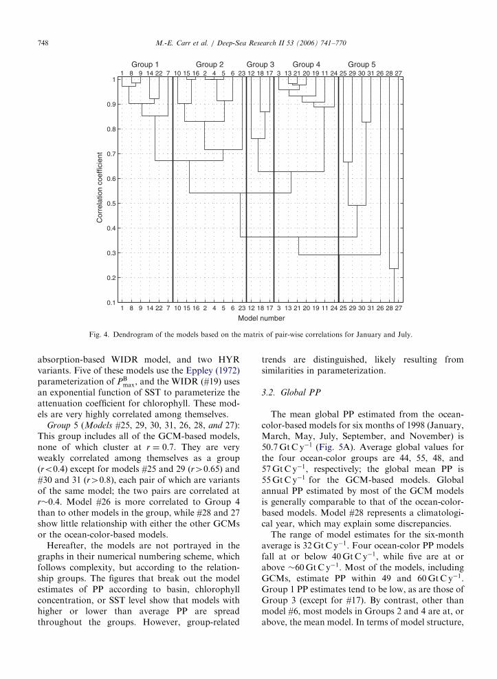
A cluster analysis (Middleton, 2000) was carriedout with the correlation matrix to group the models(Fig. 4). The correlation matrix is reduced to asingle correlation coefficient via an iterative proce-dure: the two largest mutual correlations areidentified; these two variables are merged togetherand the other variables take on an ‘average’correlation within the reduced matrix (the un-weighted pair-group method using arithmeticaverages or UPGMA as in Rohlf, 1963). The resultsare expressed as a dendrogram. Five groups weredistinguished.
Group 1 (Models #1, 8, 9, 14, 22, and 7): Thisgroup includes the simplest model, a WRDR model,
and four WIDIs: three variants of the verticallygeneralized production model (VGPM, Behrenfeldand Falkowski, 1997a) and a model based on neuralnetworks. All the models in this group are highlycorrelated among themselves (r40:82). Four ofthe models in this group have no SST-dependence(#1, 8/9, and 22).
Group 2 (Models #10, 15, 16, 2, 4, 5, 6, and 23):This group has a WRDR model, the originalVGPM, its twin (#4), and two additional VGPMvariants (#5, 6), as well as two WIDR whichparameterize PB
opt following VGPM (#15, 16). Allmodels in this group (except for #23) are correlatedat r40:8. Group 2 is correlated to Group 1 with anr�0:65.
Group 3 (Models #12, 18, and 17): This groupincludes two WIDR models and a WIDI (a HYRvariant) which distinguishes integrated primaryproduction within and below the mixed layer(#12). Model #12 does not use SST. These modelsare correlated at r40:7 and are more correlated toGroup 4 than to the previous two groups.
Group 4 (Models #3, 13, 21, 20, 19, 11, 24): Thisgroup includes three WRDRs, a VGPM variant, an
ARTICLE IN PRESS
1 8 9 14 22 7 10 15 16 2 4 5 6 23 12 18 17 3 13 21 20 19 11 24 25 29 30 31 26 28 270.1
0.2
0.3
0.4
0.5
0.6
0.7
0.8
0.9
1
Model number
Cor
rela
tion
coef
ficie
nt
Group 1 Group 2 Group 3 Group 4 Group 51 8 9 14 22 7 10 15 16 2 4 5 6 23 12 18 17 3 13 21 20 19 11 24 25 29 30 31 26 28 27
Fig. 4. Dendrogram of the models based on the matrix of pair-wise correlations for January and July.
M.-E. Carr et al. / Deep-Sea Research II 53 (2006) 741–770748
absorption-based WIDR model, and two HYRvariants. Five of these models use the Eppley (1972)parameterization of PB
max, and the WIDR (#19) usesan exponential function of SST to parameterize theattenuation coefficient for chlorophyll. These mod-els are very highly correlated among themselves.
Group 5 (Models #25, 29, 30, 31, 26, 28, and 27):This group includes all of the GCM-based models,none of which cluster at r ¼ 0:7. They are veryweakly correlated among themselves as a group(ro0:4) except for models #25 and 29 (r40:65) and#30 and 31 (r40:8), each pair of which are variantsof the same model; the two pairs are correlated atr�0:4. Model #26 is more correlated to Group 4than to other models in the group, while #28 and 27show little relationship with either the other GCMsor the ocean-color-based models.
Hereafter, the models are not portrayed in thegraphs in their numerical numbering scheme, whichfollows complexity, but according to the relation-ship groups. The figures that break out the modelestimates of PP according to basin, chlorophyllconcentration, or SST level show that models withhigher or lower than average PP are spreadthroughout the groups. However, group-related
trends are distinguished, likely resulting fromsimilarities in parameterization.
3.2. Global PP
The mean global PP estimated from the ocean-color-based models for six months of 1998 (January,March, May, July, September, and November) is50.7GtC y�1 (Fig. 5A). Average global values forthe four ocean-color groups are 44, 55, 48, and57GtC y�1, respectively; the global mean PP is55GtC y�1 for the GCM-based models. Globalannual PP estimated by most of the GCM modelsis generally comparable to that of the ocean-color-based models. Model #28 represents a climatologi-cal year, which may explain some discrepancies.
The range of model estimates for the six-monthaverage is 32GtCy�1. Four ocean-color PP modelsfall at or below 40GtC y�1, while five are at orabove �60GtCy�1. Most of the models, includingGCMs, estimate PP within 49 and 60GtC y�1.Group 1 PP estimates tend to be low, as are those ofGroup 3 (except for #17). By contrast, other thanmodel #6, most models in Groups 2 and 4 are at, orabove, the mean model. In terms of model structure,

ARTICLE IN PRESS
1 8 9 14 22 7 10 15 16 2 4 5 6 23 12 18 17 3 13 21 20 19 11 24 25 29 30 31 26 28 2730
40
50
60
70
80
Group 1 Group 2 Group 3 Group 4 Group 5
Gt C
y-1
MEAN GLOBAL PRODUCTION 1998
1 8 9 14 22 7 10 15 16 2 4 5 6 23 12 18 17 3 13 21 20 19 11 24 25 29 30 31 26 28 27-2
0
2
4
6
% D
iffer
ence
DIFFERENCE BETWEEN DECEMBER 98 and 99
WIDRWRDR
WIDI
GCM
Group 1 Group 2 Group 3 Group 4 Group 5
WIDRWRDR
WIDI
GCM
(A)
(B)
Fig. 5. The annual mean primary production for each model for 1998 (A) and a comparison between December of 1998 and December of
1999 (B). The models are ordered following the groups obtained from the cluster analysis and the five groups are separated by vertical
lines. The horizontal line is the annual global production for the ocean-color-mean model (A) and the percent increase from December
1998 to December 1999 (B) for the ocean-color-mean model.
M.-E. Carr et al. / Deep-Sea Research II 53 (2006) 741–770 749
the VGPM variants are consistently close to theaverage model value with the exception of #6, whichis low (Fig. 5A). The broadest range is observedamong the WIDR models (#17 is very high while#18 is low) and the non-VGPM WIDI models (#13is high, while #12 and 14 are low).
The observed range of values for global produc-tion (Fig. 5A) is comparable to that obtained fromextrapolations of field measurements, such as thoseof Koblentz-Mishke et al. (1970) or Berger (1989),but it would be a mistake to interpret this as a lackof progress. Rather, the similarity lends credibilityto our understanding of global marine photosynth-esis. Ocean-color-based models allow us to docu-ment spatial and temporal variability on scales thatare inaccessible to field programs.
We compared December 1998 with December1999 to see if the models consistently capturedvariability between the two years (Fig. 5B). GlobalPP estimated by the ocean-color-based models isuniformly larger in December 1999 than in 1998 byon average 3%. Model #27 was the only GCM-based model that estimated a comparable difference
between the two Decembers to that of the ocean-color-based models (not surprising since forcingfields for interannual variability in the GCM-basedmodels were different). The observed increase in PPlikely results from the observed increase in bothchlorophyll concentration and PAR in December of1999 relative to December 1998.
3.3. Basin PP
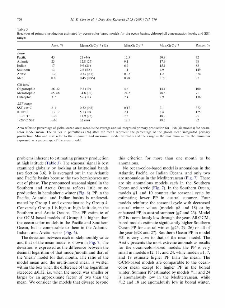
We divided the world ocean into basins followingAntoine et al. (1996) with the mask available athttp://marine.rutgers.edu/opp/Mask/MASK1.html.The integrated PP in each basin is proportional tothe basin areal extent in the Pacific, while theAtlantic and Indian tend to be slightly moreproductive and the Southern and Arctic Oceanstend to be less productive (Table 3). Thesedifferences are consistent with basin average lati-tude and the corresponding insolation. In all basins,the range between model estimates is as large as themean; in the case of the Arctic Ocean, it is almosttwice as large, reflecting both the small area and the
ARTICLE IN PRESS
Table 3
Breakout of primary production estimated by ocean-color-based models for the ocean basins, chlorophyll concentration levels, and SST
ranges
Area, % Mean/GtCy�1 (%) Min/GtCy�1 Max/GtCy�1 Range, %
Basin
Pacific 45 21 (44) 15.5 30.9 72
Atlantic 23 12.8 (27) 9.1 17.9 68
Indian 17 9.9 (21) 6.9 15.1 83
Southern 13 2.6 (5.5) 1.1 4.9 149
Arctic 1.2 0.33 (0.7) 0.02 1.2 374
Med. 0.8 0.45 (0.95) 0.28 0.73 97
Chl level
Oligotrophic 26–32 9.2 (19) 4.6 14.1 100
Mesotrophic 65–68 34.8 (70) 24.2 48.8 71
Eutrophic 3–5 5.6 (11) 2.4 9.9 136
SST range
SSTo0 �C 2–4 0.52 (0.8) 0.17 2.1 372
0–10 �C 13–17 5.1 (10) 2.1 8.4 125
10–20 �C �20 11.9 (25) 7.6 18.9 95
420 �C SST �60 32 (64) 19.1 48.7 92
Area refers to percentage of global ocean area; mean is the average annual integrated primary production for 1998 (six months) for ocean-
color model mean. The values in parenthesis (%) after the mean represent the percentage of the global mean integrated primary
production. Min and max refer to the minimum and maximum model estimates and the range is the maximum minus the minimum
expressed as a percentage of the mean model.
M.-E. Carr et al. / Deep-Sea Research II 53 (2006) 741–770750
problems inherent to estimating primary productionat high latitude (Table 3). The seasonal signal is bestexamined globally by looking at latitudinal bands(see Section 3.6); it is averaged out in the Atlanticand Pacific basins because the two hemispheres areout of phase. The pronounced seasonal signal in theSouthern and Arctic Oceans reflects little or noproduction in hemispheric winter (Fig. 6). PP in thePacific, Atlantic, and Indian basins is underesti-mated by Group 1 and overestimated by Group 4.Conversely Group 1 is high at high latitude, in theSouthern and Arctic Oceans. The PP estimate ofthe GCM-based models of Group 5 is higher thanthe ocean-color models in the Pacific and SouthernOcean, but is comparable to them in the Atlantic,Indian, and Arctic basins (Fig. 6).
The deviation between each model/monthly valueand that of the mean model is shown in Fig. 7. Thedeviation is expressed as the difference between thedecimal logarithm of that model/month and that ofthe ‘mean’ model for that month. The ratio of themodel mean and the multi-model mean is writtenwithin the box when the difference of the logarithmsexceeded �0:32, i.e. when the model was smaller orlarger by an approximate factor of two than themean. We consider the models that diverge beyond
this criterion for more than one month to beanomalous.
No ocean-color-based model is anomalous in theAtlantic, Pacific, or Indian Oceans, and only twoare anomalous in the Mediterranean (Fig. 7). Thereare six anomalous models each in the SouthernOcean and Arctic (Fig. 7). In the Southern Ocean,models #1 and 10 counter the seasonal cycle byestimating lower PP in austral summer. Fourmodels reinforce the seasonal cycle with decreasedaustral winter values (models #8 and 18) or byenhanced PP in austral summer (#7 and 23). Model#12 is anomalously low through the year. All GCM-based models estimate significantly higher SouthernOcean PP for austral winter (#25, 29, 26) or all ofthe year (#28 and 27). Southern Ocean PP in model#31 is very close to that of the mean model. TheArctic presents the most extreme anomalous resultsfor the ocean-color-based models: the PP is verysmall in models #12, 11, and 24, while models #1, 7,and 19 estimate higher PP than the mean. TheGCM-based models are comparable to the ocean-color mean except for higher PP in the borealwinter. Summer PP estimated by models #11 and 24is anomalously low in the Mediterranean, while#12 and 18 are anomalously low in boreal winter.

ARTICLE IN PRESS
1 3 5 7 9 1110
15
20
25
PACIFIC
Gt C
y-1
1 3 5 7 9 116
8
10
12
14
16
18
ATLANTIC
1 3 5 7 9 114
6
8
10
12
14
INDIAN
1 3 5 7 9 110
2
4
6
8 G1G2G3G4G5
SOUTHERN OCEAN
Month of 1998
Gt C
y-1
1 3 5 7 9 11
0
0.2
0.4
0.6
0.8
1
1.2
ARCTIC
Month of 19981 3 5 7 9 11
0
0.2
0.4
0.6
0.8
MEDITERRANEAN
Month of 1998
Fig. 6. The monthly progression of the PP (expressed as an annual value) within each basin for the ocean-color-mean model (thick line)
and the monthly average of each of the five groups, denoted here as G1 through G5. Note that the range of area-averaged PP changes in
each basin/panel.
M.-E. Carr et al. / Deep-Sea Research II 53 (2006) 741–770 751
GCM-based models #26, 30 and 31 have noMediterranean basin, and the other models ofGroup 5 generally underestimate PP in this basin,especially in winter months.
3.4. Chlorophyll concentration levels
We divided the global fields into levels of chlorophyllconcentration, i.e. oligotrophic (o0:1mgChlm�3),mesotrophic (0.1–1mgChlm�3), and eutrophicwaters (41mgChlm�3), to evaluate the modelperformance for these conditions (Fig. 8).Although, there is a variable apportioning in eachcategory from month to month, concentrations areconsistently less than 1mgChlm�3 for �95% of theocean (Table 3). As expected from the area, the bulkof global PP occurs in mesotrophic waters,�35GtC y�1, or 70% (Fig. 8 and Table 3).Integrated PP in eutrophic waters is about half thatof oligotrophic ones, although their area is 6–10times smaller (Fig. 8 and Table 3). The normalizedrange between models varies most for eutrophicwaters (Table 3 and Fig. 8). Systematic differencesbetween the groups can be distinguished among the
chlorophyll concentration levels. PP estimated byGroup 1 is much lower than the mean in oligo-trophic and mesotrophic regions, while that ofGroup 3 is lower than the mean model for eutrophicwaters, but is higher than the mean in oligotrophicwaters. Since the majority of global PP occurs inmesotrophic regions, this explains why Group 1estimates lower global PP than the mean model(Figs. 5 and 8). Groups 2 and 4 have higher PP inmesotrophic, and Group 4 is much higher undereutrophic conditions.
It should be noted that the GCM-based modelsdo not use ocean color, so the eutrophic areas formodels #1 through 24 are unlikely to coincide withmodels 25 through 29. We compared the chlor-ophyll fields for models #25 and 29 with the inputfields used here. The area in which chlorophyllconcentrations are eutrophic is 30% (#29) to 60%(#25) smaller than in the SeaWiFS fields. Theoligotrophic and mesotrophic areas are within10% for #25 though the oligotrophic area is 50%larger in #29. PP from Group 5 is higher thanthe ocean-color mean when chlorophyll is less than0.1mgChlm�3, while it is much lower in eutrophic

ARTICLE IN PRESS
1 3 5 7 9 11
4
6
8
10
12
14OLIGOTROPHIC
Month of 1998
Gt C
y-1
1 3 5 7 9 11
20
25
30
35
40
45MESOTROPHIC
Month of 19981 3 5 7 9 11
2
4
6
8
10G1G2G3G4G5
EUTROPHIC
Month of 1998
Fig. 8. The monthly progression of the PP (expressed as an annual value) within each chlorophyll level for the ocean-color-mean model
(thick line) and the monthly average of each of the five groups, denoted here as G1 through G5. The chlorophyll levels are oligotrophic
ðo0:1mgChlm�3Þ, mesotrophic (0.1–1mgChlm�3), and eutrophic ð41mgChlm�3Þ. Note that the range of area-averaged PP changes in
each chlorophyll level/panel.
PACIFIC98019805980998129912
0.50.30.30.4
ATLANTIC98019805980998129912
0.40.30.30.40.5
INDIAN98019805980998129912
2.1 0.4 0.4 3 2.60.4 0.4 3.3 2.5
3.4 0.5 2.8 0.4 0.2 2.7 2.8 16 53.3 0.4 6 0.3 0.1 0.5 4.5 2.7 3.7 42 4.52.6 0.4 0.4 2.4 2.3 2.7 8.9 5.8
2.1 0.4 2.2 4.9 4.52.1 0.4 0.5 3.5 3.7
0.4 2.1 3.5 3.8
SOUTHERN OCEAN98019805980998129912
722.9 3.8 0.2 3.1 4.9
3.9 0.1 0.2 0.10.5 3.6 0.1
2.5 2.8 0.1 0.3 0.1 0.1 0.30.1 0.4 9.5
ARCTIC98019805980998129912
0.4 0.4 0.3 0.40.4
0.3 0.4 0.4 0.3 0.40.2 0.5 0.4 0.30.3 0.3
0.4 0.4 0.2 0.30.4 0.5 0.4 0.2 0.30.4 0.5 0.2 0.3
MEDITERRANEAN
Group 1 Group 2 Group 3 Group 4 Group 51 8 9 14 22 7 10 15 16 2 4 5 6 23 12 18 17 3 13 21 20 19 11 24 25 29 30 31 26 28 27
98019805980998129912
log1
0(P
Pi)-
mea
n(lo
g10(
PP
))
1
-0.8
-0.6
-0.4
-0.2
0
0.2
0.4
0.6
0.8
1
Fig. 7. Comparison between monthly PP of each model within each basin and that of the ocean-color-mean model. Models are ordered
following the dendrogram and the five groups are separated by vertical lines. The horizontal line separates the six months of 1998 from
December 1998 and 1999. When the comparison exceeds a factor of two, the ratio is written within the box. A white box denotes missing
data or very small numbers.
M.-E. Carr et al. / Deep-Sea Research II 53 (2006) 741–770752
regions. This is consistent with the GCMs havingfewer very high values.
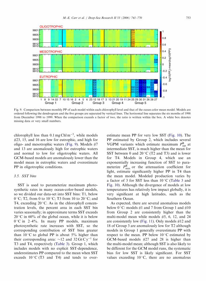
Model output diverges most for low and highchlorophyll concentration levels, but there is onlyone anomalous ocean-color model in eutrophic
waters (#12, Fig. 9). Although the differences areless than a factor of two from the mean model, thereare distinct tendencies in some models and groups.For example, model #6 is low for mesotrophic andeutrophic waters but close to the mean for
ARTICLE IN PRESS
2.42.32.12.12.22.42.52.3
OLIGOTROPHIC9801
9805
9809
98129912
0.40.4
MESOTROPHIC9801
9805
9809
98129912
0.4 0.4 0.2 0.2 0.4 0.20.4 0.4 0.2 0.2 0.3 0.10.4 0.4 0.2 0.3 0.40.4 0.4 0.4 0.2 0.2 0.4 0.40.4 0.5 0.4 0.2 0.2 0.30.4 0.5 0.4 0.2 0.2 0.4 0.20.4 0.5 0.2 0.3 0.5 0.30.4 0.4 0.3 0.4 0.3
EUTROPHIC
Group 1 Group 2 Group 3 Group 4 Group 51 8 9 14 22 7 10 15 16 2 4 5 6 23 12 18 17 3 13 21 20 19 11 24 25 29 30 31 26 28 27
9801
9805
9809
98129912
log1
0(P
Pi)-
mea
n(lo
g10(
PP
))
-1
-0.8
-0.6
-0.4
-0.2
0
0.2
0.4
0.6
0.8
1
Fig. 9. Comparison between monthly PP of each model within each chlorophyll level and that of the ocean color mean model. Models are
ordered following the dendrogram and the five groups are separated by vertical lines. The horizontal line separates the six months of 1998
from December 1998 to 1999. When the comparison exceeds a factor of two, the ratio is written within the box. A white box denotes
missing data or very small numbers.
M.-E. Carr et al. / Deep-Sea Research II 53 (2006) 741–770 753
chlorophyll less than 0.1mgChlm�3, while models#23, 15, and 16 are low for eutrophic, and high foroligo- and mesotrophic waters (Fig. 9). Models #7and 13 are anomalously high for eutrophic watersand normal to low for oligotrophic waters. AllGCM-based models are anomalously lower than themodel mean in eutrophic waters and overestimatePP in oligotrophic conditions.
3.5. SST bins
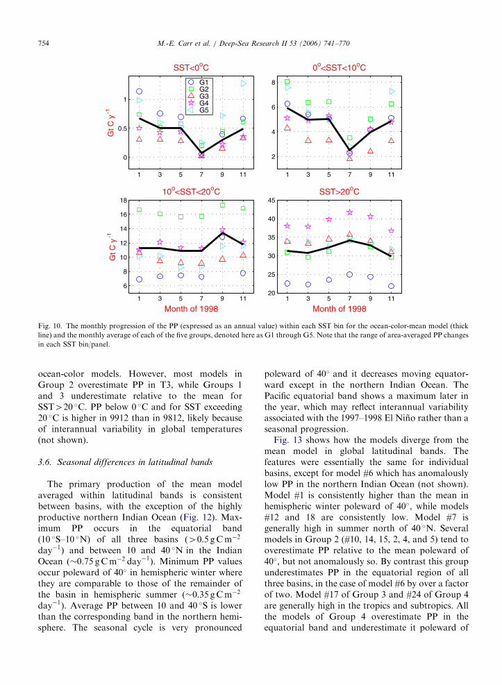
SST is used to parameterize maximum photo-synthetic rates in many ocean-color-based models,so we divided our data-set into SST bins: T1, below0 �C; T2, from 0 to 10 �C; T3 from 10 to 20 �C; andT4, exceeding 20 �C. As in the chlorophyll concen-tration levels, the percent area in each SST binvaries seasonally; in approximate terms SST exceeds20 �C in 60% of the global ocean, while it is below0 �C in 2–4%. In many PP models, maximumphotosynthetic rate increases with SST, so thecorresponding contribution of SST bins greaterthan 10 �C to global PP is about 5% higher thantheir corresponding area: �12 and 32GtC y�1 forT3 and T4, respectively (Table 3). Group 1, whichincludes models with no explicit SST-dependence,underestimates PP compared to the mean when SSTexceeds 10 �C (T3 and T4) and tends to over-
estimate mean PP for very low SST (Fig. 10). ThePP estimated by Group 2, which includes severalVGPM variants which estimate maximum PB
opt atintermediate SST, is much higher than the mean forSST between 0 and 20 �C (T2 and T3) and is lowerfor T4. Models in Group 4, which use anexponentially increasing function of SST to para-meterize PB
max or the attenuation coefficient forlight, estimate significantly higher PP in T4 thanthe mean model. Modeled production varies bya factor of 3 for SST less than 10 �C (Table 3 andFig. 10). Although the divergence of models at lowtemperatures has relatively low impact globally, it isvery significant at high latitudes, such as theSouthern Ocean.
As expected, there are several anomalous modelsbelow 0 �C: models #1 and 7 from Group 1 and #10from Group 2 are consistently higher than themulti-model mean while models #5, 6, 12, and 24are consistently low (Fig. 11). Only models #12 and18 of Group 3 are anomalously low for T2 althoughmodels in Group 1 generally overestimate PP withrespect to the mean. PP below 10 �C estimated byGCM-based models #27 and 28 is higher thanthe multi-model mean; although SST is also likely tobe different for the GCMmodel runs, the systematicbias for low SST is likely significant. For SSTvalues exceeding 10 �C, there are no anomalous
ARTICLE IN PRESS
1 3 5 7 9 11
0
0.5
1
G1G2G3G4G5
SST<0oC
Gt C
y-1
1 3 5 7 9 11
2
4
6
8
0o<SST<10oC
1 3 5 7 9 11
6
8
10
12
14
16
1810o<SST<20oC
Month of 1998
Gt C
y-1
1 3 5 7 9 1120
25
30
35
40
45SST>20oC
Month of 1998
Fig. 10. The monthly progression of the PP (expressed as an annual value) within each SST bin for the ocean-color-mean model (thick
line) and the monthly average of each of the five groups, denoted here as G1 through G5. Note that the range of area-averaged PP changes
in each SST bin/panel.
M.-E. Carr et al. / Deep-Sea Research II 53 (2006) 741–770754
ocean-color models. However, most models inGroup 2 overestimate PP in T3, while Groups 1and 3 underestimate relative to the mean forSST420 �C. PP below 0 �C and for SST exceeding20 �C is higher in 9912 than in 9812, likely becauseof interannual variability in global temperatures(not shown).
3.6. Seasonal differences in latitudinal bands
The primary production of the mean modelaveraged within latitudinal bands is consistentbetween basins, with the exception of the highlyproductive northern Indian Ocean (Fig. 12). Max-imum PP occurs in the equatorial band(10 �S–10 �N) of all three basins (40:5 gCm�2
day�1) and between 10 and 40 �N in the IndianOcean (�0.75 gCm�2 day�1). Minimum PP valuesoccur poleward of 40� in hemispheric winter wherethey are comparable to those of the remainder ofthe basin in hemispheric summer (�0:35 gCm�2
day�1). Average PP between 10 and 40 �S is lowerthan the corresponding band in the northern hemi-sphere. The seasonal cycle is very pronounced
poleward of 40� and it decreases moving equator-ward except in the northern Indian Ocean. ThePacific equatorial band shows a maximum later inthe year, which may reflect interannual variabilityassociated with the 1997–1998 El Nino rather than aseasonal progression.
Fig. 13 shows how the models diverge from themean model in global latitudinal bands. Thefeatures were essentially the same for individualbasins, except for model #6 which has anomalouslylow PP in the northern Indian Ocean (not shown).Model #1 is consistently higher than the mean inhemispheric winter poleward of 40�, while models#12 and 18 are consistently low. Model #7 isgenerally high in summer north of 40 �N. Severalmodels in Group 2 (#10, 14, 15, 2, 4, and 5) tend tooverestimate PP relative to the mean poleward of40�, but not anomalously so. By contrast this groupunderestimates PP in the equatorial region of allthree basins, in the case of model #6 by over a factorof two. Model #17 of Group 3 and #24 of Group 4are generally high in the tropics and subtropics. Allthe models of Group 4 overestimate PP in theequatorial band and underestimate it poleward of

ARTICLE IN PRESS
3.9 2.6 0.2 0.3 0.4 0.2 32.9 2.8 2.2 0.3 0.4 0.3 2.32.2 4.7 4.3 0.4 0.4 0.2 0.4 2.6 0.3 0.2 0.3 2.7
0.1 0.2 2.5 15 0.1 0.1 0.1 0.1 0.1 0.1 0.2 0.1 0.1 0.2 0.2 0.2 2.1 0.3 15 2.22.7 2.5 5.1 0.4 0.4 0.2 0.5 0.4 2.1 0.1 2.1 5.3 4.7
2.6 3.6 0.4 0.4 0.3 0.4 2.2 4.3 5.83.4 4.5 0.5 0.4 0.2 0.2 0.4 0.2 2.4 2.5 4.4 5.8
2.7 0.5 2.2 0.3 0.3 0.3 0.5 0.3 0.2 5.2 4.9 3 2.3 7.2 8.9
SST<0oC9801
9805
9809
98129912
0.4 2.20.4 0.4
2.1 0.42.9 0.4
0.4 0.50.4 2.40.4 2.10.4 2.2
0o<SST<10oC9801
9805
9809
98129912
0.40.30.20.20.20.40.4
10o<SST<20oC9801
9805
9809
98129912
0.5
SST>20oC
Group 1 Group 2 Group 3 Group 4 Group 51 8 9 14 22 7 10 15 16 2 4 5 6 23 12 18 17 3 13 21 20 19 11 24 25 29 30 31 26 28 27
9801
9805
9809
98129912
log1
0(P
Pi)-
mea
n(lo
g10(
PP
))
-1
-0.8
-0.6
-0.4
-0.2
0
0.2
0.4
0.6
0.8
1
Fig. 11. Comparison between monthly PP of each model within each SST bin and that of the ocean-color-mean model. Models are
ordered following the dendrogram and the five groups are separated by vertical lines. The horizontal line separates the six months of 1998
from December 1998 and 1999. When the comparison exceeds a factor of two, the ratio is written within the box. A white box denotes
missing data or very small numbers.
1 3 5 7 9 110
0.2
0.4
0.6
0.8
Pacific Basin
Months of 1998
>40oN10o -40oN10o S-10oN10o -40oS<40o S
gC m
-2 d
ay-1
1 3 5 7 9 110
0.2
0.4
0.6
0.8
Atlantic Basin
Months of 19981 3 5 7 9 11
0
0.2
0.4
0.6
0.8
Indian Basin
Months of 1998
Fig. 12. Monthly progression of area-integrated PP (expressed as an annual value) of the ocean-color-mean model within latitudinal
bands in each basin.
M.-E. Carr et al. / Deep-Sea Research II 53 (2006) 741–770 755
40�. The GCM-based models, especially model #27,tend to overestimate ocean-color mean PP in theequatorial region. Models #27 and 28 obtain higherPP than does the mean ocean-color model polewardof 40 �S, while #30 and 31 underestimate PPpoleward of 40 �N.
3.7. Sensitivity analysis
This analysis examines the effect of the inputvariables on the ocean-color-based determination ofprimary production. The GCM-based models didnot carry out this exercise as they do not use the

ARTICLE IN PRESS
>40oN2.7 0.3 0.3 2.2
0.4 0.52.1 0.4
0.4 0.4 0.40.3 0.4
2.2 0.4 0.3 0.42.7 0.3 0.3 0.42.6 0.3 0.3 0.4
98019805980998129912
10o-40 oN98019805980998129912
10oS-10 oN
Mon
th
0.4 2.40.4 0.4 2.2 2.90.5 0.4 2.3
0.5 2.20.4 2.40.5 2.50.5 2.50.5 2.3
98019805980998129912
10oS-40 oS98019805980998129912
<40oS2.1 2.22.2 2.1
2.3 0.4 0.3 4.5 2.52.4 0.4 0.3 6.2 2.2
0.5 0.5 3.5 2.80.5 2.6 3
2.3 2.52.2 2.5
Group 1 Group 2 Group 3 Group 4 Group 51 8 9 14 22 7 10 15 16 2 4 5 6 23 12 18 17 3 13 21 20 19 11 24 25 29 30 31 26 28 27
98019805980998129912
log1
0(P
Pi)-
mea
n(lo
g10(
PP
))
-1
-0.8
-0.6
-0.4
-0.2
0
0.2
0.4
0.6
0.8
1
Fig. 13. Comparison between monthly PP of each model within latitudinal bands and that of the ocean-color-mean model. Models are
ordered following the dendrogram and the five groups are separated by vertical lines. The horizontal line separates the six months of 1998
from December 1998 and 1999. When the comparison exceeds a factor of two, the ratio is written within the box. A white box denotes
missing data or very small numbers.
M.-E. Carr et al. / Deep-Sea Research II 53 (2006) 741–770756
input fields nor is it trivial to change the forcingvalues at specific locations. Starting with the 11‘representative’ points of Table 2 and Fig. 2, wesystematically varied the mixed-layer depth, SST,PAR, and chlorophyll concentration within a rangeof reasonable values, holding the other inputvariables at their original magnitude. We then plotthe impact in simulated primary production (DPP)at each location corresponding to the change in eachof the four input variables for each model, (DMLD,DSST, DPAR, and DChl). Because the variation inthe input variables is unrealistic for some locations,we have reduced the axes of the plots to correspondto the observed range of input variables at the studypoints. We only show the most extreme andcharacteristic points in these plots (points 1, 2, 4,7, 8, 10, and 11) that are evenly distributed betweenJanuary and July (Table 2). A subset of ocean-color-based models have contributed to part 2(Table 1).
Only six models use mixed-layer depth (Fig. 14;models #14 of Group 1, #23 of Group 2, #12 of
Group 3, and #20, 11, and 24 of Group 4). Theimpact of changing mixed-layer depth is less than afactor of two except for model #11 (which integratesto mixed-layer depth instead of to euphotic depth)where PP almost triples in response to increasedmixed-layer depth. In two models (#11 and 14)deepening mixed layers increases PP asymptotically.Models #20 and #23 are insensitive to DMLD.Model #12 shows maximum impact for changes oforder 50m, which primarily lead to decreases in PP.Model #24 presents peak DPP at DMLD of75–100m, which then decreases for deeper mixedlayers. In model #20, DPP is weakly negative forpositive DMLD, while model #23 responds primar-ily, if weakly, to negative DMLD. Points 10, 11, and8 are most sensitive; these points have shallow initialmixed-layer depths (Fig. 2 and Table 2).
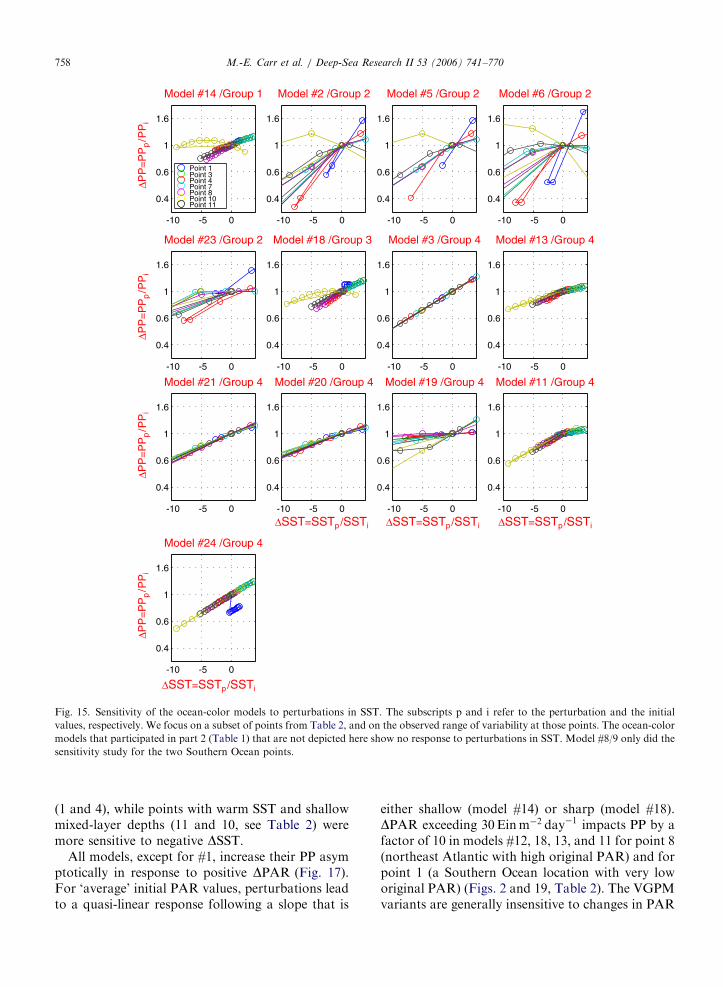
All models except for #1, 8/9, and 22 (in Group 1)and #12 (Group 3) use SST (Fig. 15). There seem tobe four responses to SST perturbations, whichcan be seen best for the full range of perturbation(Fig. 16): a gaussian shape (#2/4, 5, 6), a linear

ARTICLE IN PRESS
-50 0 50 100 150 2000.4
0.6
1
1.6
2.5
3.9
Model #14 /Group 1
∆PP
=P
Pp/P
Pi
∆PP
=P
Pp/P
Pi
∆PP
=P
Pp/P
Pi
∆MLD=MLDp-MLDi ∆MLD=MLDp-MLDi
-50 0 50 100 150 2000.4
0.6
1
1.6
2.5
3.9
Model #23 /Group 2
Point 1Point 3Point 4Point 7Point 8Point 10Point 11
-50 0 50 100 150 2000.4
0.6
1
1.6
2.5
3.9
Model #12 /Group 3
-50 0 50 100 150 2000.4
0.6
1
1.6
2.5
3.9
Model #20 /Group 4
-50 0 50 100 150 2000.4
0.6
1
1.6
2.5
3.9
Model #11 /Group 4
-50 0 50 100 150 2000.4
0.6
1
1.6
2.5
3.9
Model #24 /Group 4
Fig. 14. Sensitivity of the ocean-color models to perturbations in mixed-layer depth. The subscripts p and i refer to the perturbation and
the initial values, respectively. We focus on a subset of points from Table 2, and on the observed range of variability at those points. The
ocean-color models that participated in part 2 (Table 1) that are not depicted here show no response to perturbations in mixed-layer depth.
Model #8/9 only did the sensitivity study for the two Southern Ocean points.
M.-E. Carr et al. / Deep-Sea Research II 53 (2006) 741–770 757
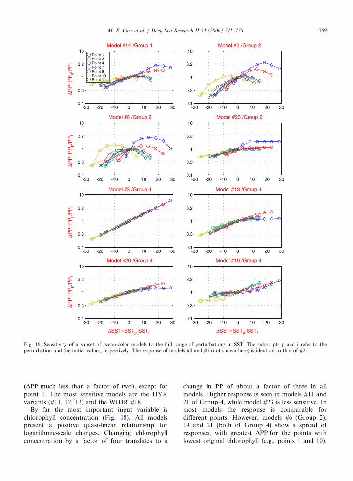
increase (#3, 20, 21, and 24), an asymptotic-linearform (#11, 13, 17, 18, and 23), and finally, in model#19, DPP increases weakly for decreasing negativeDSST to an inflection point (not always 0 �C) afterwhich it increases more sharply. The Gaussianshape results from the polynomial function of SSTused in the VGPM and some of its variants;maximum DPP occurs at SST�20 �C for Model#2/4, or 5 and at �15 �C for Model #6 (Fig. 16).
The models that have a linear or asymptoticresponse consistently have negative DPP for nega-tive DSST. By contrast, the models with a centralmaximum present peak DPP at both positive andnegative DSST for different points (Fig. 16). Akey difference between model responses seems tobe whether DPP increases with positive DSST(Group 4). The points that were most sensitiveto positive DSST are points with low initial SST
ARTICLE IN PRESS
-10 -5 0
0.4
0.6
1
1.6
Model #14 /Group 1
Point 1Point 3Point 4Point 7Point 8Point 10Point 11
∆PP
=P
Pp/P
Pi
∆PP
=P
Pp/P
Pi
∆PP
=P
Pp/P
Pi
∆SST=SSTp/SSTi
∆SST=SSTp/SSTi ∆SST=SSTp/SSTi ∆SST=SSTp/SSTi
∆PP
=P
Pp/P
Pi
-10 -5 0
0.4
0.6
1
1.6
Model #2 /Group 2
-10 -5 0
0.4
0.6
1
1.6
Model #5 /Group 2
-10 -5 0
-10 -5 0 -10 -5 0 -10 -5 0 -10 -5 0
-10 -5 0
-10 -5 0
-10 -5 0 -10 -5 0 -10 -5 0
0.4
0.6
1
1.6
Model #6 /Group 2
0.4
0.6
1
1.6
Model #23 /Group 2
0.4
0.6
1
1.6
Model #18 /Group 3
0.4
0.6
1
1.6
Model #3 /Group 4
0.4
0.6
1
1.6
Model #13 /Group 4
0.4
0.6
1
1.6
Model #21 /Group 4
0.4
0.6
1
1.6
Model #20 /Group 4
0.4
0.6
1
1.6
Model #19 /Group 4
0.4
0.6
1
1.6
Model #11 /Group 4
0.4
0.6
1
1.6
Model #24 /Group 4
Fig. 15. Sensitivity of the ocean-color models to perturbations in SST. The subscripts p and i refer to the perturbation and the initial
values, respectively. We focus on a subset of points from Table 2, and on the observed range of variability at those points. The ocean-color
models that participated in part 2 (Table 1) that are not depicted here show no response to perturbations in SST. Model #8/9 only did the
sensitivity study for the two Southern Ocean points.
M.-E. Carr et al. / Deep-Sea Research II 53 (2006) 741–770758
(1 and 4), while points with warm SST and shallowmixed-layer depths (11 and 10, see Table 2) weremore sensitive to negative DSST.
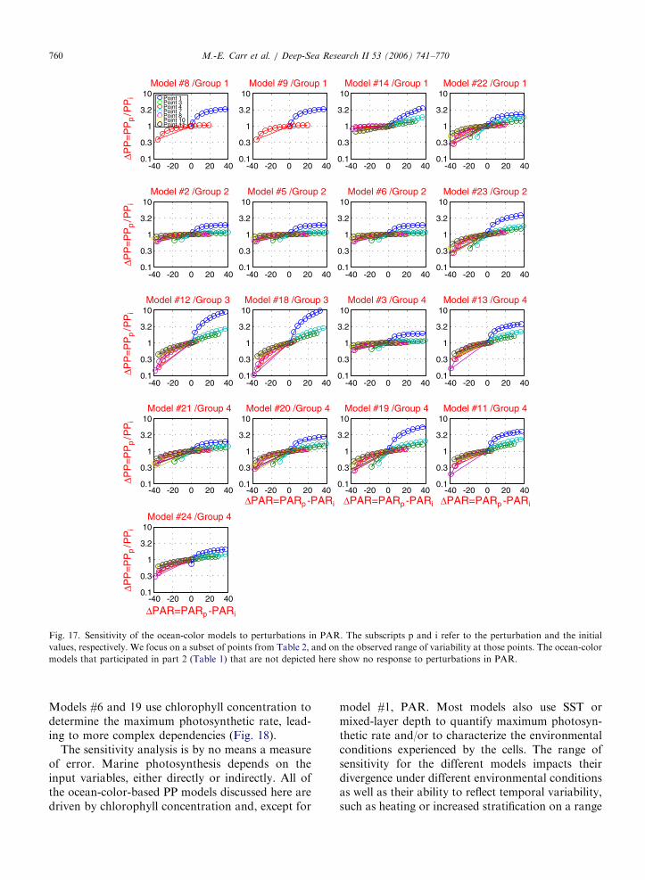
All models, except for #1, increase their PP asymptotically in response to positive DPAR (Fig. 17).For ‘average’ initial PAR values, perturbations leadto a quasi-linear response following a slope that is
either shallow (model #14) or sharp (model #18).DPAR exceeding 30Einm�2 day�1 impacts PP by afactor of 10 in models #12, 18, 13, and 11 for point 8(northeast Atlantic with high original PAR) and forpoint 1 (a Southern Ocean location with very loworiginal PAR) (Figs. 2 and 19, Table 2). The VGPMvariants are generally insensitive to changes in PAR
ARTICLE IN PRESS
-30 -20 -10 0 10 20 30 -30 -20 -10 0 10 20 30
-30 -20 -10 0 10 20 30 -30 -20 -10 0 10 20 30
-30 -20 -10 0 10 20 30 -30 -20 -10 0 10 20 30
-30 -20 -10 0 10 20 30 -30 -20 -10 0 10 20 30
0.1
0.3
1
3.2
10Model #14 /Group 1
Point 1Point 3Point 4Point 7Point 8Point 10Point 11
0.1
0.3
1
3.2
10Model #2 /Group 2
0.1
0.3
1
3.2
10Model #6 /Group 2
0.1
0.3
1
3.2
10Model #23 /Group 2
0.1
0.3
1
3.2
10Model #3 /Group 4
0.1
0.3
1
3.2
10Model #13 /Group 4
0.1
0.3
1
3.2
10Model #20 /Group 4
0.1
0.3
1
3.2
10Model #19 /Group 4
∆SST=SSTp-SSTI∆SST=SSTp-SSTI
∆PP
=P
Pp/
PP
I∆P
P=
PP
p/P
PI
∆PP
=P
Pp/
PP
I∆P
P=
PP
p/P
PI
Fig. 16. Sensitivity of a subset of ocean-color models to the full range of perturbations in SST. The subscripts p and i refer to the
perturbation and the initial values, respectively. The response of models #4 and #5 (not shown here) is identical to that of #2.
M.-E. Carr et al. / Deep-Sea Research II 53 (2006) 741–770 759
(DPP much less than a factor of two), except forpoint 1. The most sensitive models are the HYRvariants (#11, 12, 13) and the WIDR #18.
By far the most important input variable ischlorophyll concentration (Fig. 18). All modelspresent a positive quasi-linear relationship forlogarithmic-scale changes. Changing chlorophyllconcentration by a factor of four translates to a
change in PP of about a factor of three in allmodels. Higher response is seen in models #11 and21 of Group 4, while model #23 is less sensitive. Inmost models the response is comparable fordifferent points. However, models #6 (Group 2),19 and 21 (both of Group 4) show a spread ofresponses, with greatest DPP for the points withlowest original chlorophyll (e.g., points 1 and 10).
ARTICLE IN PRESS
-40 -20 0 20 40 -40 -20 0 20 40 -40 -20 0 20 40 -40 -20 0 20 40
-40 -20 0 20 40 -40 -20 0 20 40 -40 -20 0 20 40 -40 -20 0 20 40
-40 -20 0 20 40 -40 -20 0 20 40 -40 -20 0 20 40 -40 -20 0 20 40
-40 -20 0 20 40
-40 -20 0 20 40
-40 -20 0 20 40 -40 -20 0 20 40 -40 -20 0 20 40
0.1
0.3
1
3.2
10Model #8 /Group 1
Point 1Point 3Point 4Point 7Point 8Point 10Point 11
∆PP
=P
Pp
/PP
i∆P
P=
PP
p/P
Pi
∆PP
=P
Pp
/PP
i∆P
P=
PP
p/P
Pi
∆PAR=PARp -PARi
∆PAR=PARp -PARi ∆PAR=PARp -PARi ∆PAR=PARp -PARi
∆PP
=P
Pp
/PP
i
0.1
0.3
1
3.2
10Model #9 /Group 1
0.1
0.3
1
3.2
10Model #14 /Group 1
0.1
0.3
1
3.2
10Model #22 /Group 1
0.1
0.3
1
3.2
10Model #2 /Group 2
0.1
0.3
1
3.2
10Model #5 /Group 2
0.1
0.3
1
3.2
10Model #6 /Group 2
0.1
0.3
1
3.2
10Model #23 /Group 2
0.1
0.3
1
3.2
10Model #12 /Group 3
0.1
0.3
1
3.2
10Model #18 /Group 3
0.1
0.3
1
3.2
10Model #3 /Group 4
0.1
0.3
1
3.2
10Model #13 /Group 4
0.1
0.3
1
3.2
10Model #21 /Group 4
0.1
0.3
1
3.2
10Model #20 /Group 4
0.1
0.3
1
3.2
10Model #19 /Group 4
0.1
0.3
1
3.2
10Model #11 /Group 4
0.1
0.3
1
3.2
10Model #24 /Group 4
Fig. 17. Sensitivity of the ocean-color models to perturbations in PAR. The subscripts p and i refer to the perturbation and the initial
values, respectively. We focus on a subset of points from Table 2, and on the observed range of variability at those points. The ocean-color
models that participated in part 2 (Table 1) that are not depicted here show no response to perturbations in PAR.
M.-E. Carr et al. / Deep-Sea Research II 53 (2006) 741–770760
Models #6 and 19 use chlorophyll concentration todetermine the maximum photosynthetic rate, lead-ing to more complex dependencies (Fig. 18).
The sensitivity analysis is by no means a measureof error. Marine photosynthesis depends on theinput variables, either directly or indirectly. All ofthe ocean-color-based PP models discussed here aredriven by chlorophyll concentration and, except for
model #1, PAR. Most models also use SST ormixed-layer depth to quantify maximum photosyn-thetic rate and/or to characterize the environmentalconditions experienced by the cells. The range ofsensitivity for the different models impacts theirdivergence under different environmental conditionsas well as their ability to reflect temporal variability,such as heating or increased stratification on a range

ARTICLE IN PRESS
0.25 0.5 1 2 40.1
0.3
1
3.2
Model #1 /Group 1
Point 1Point 3Point 4Point 7Point 8Point 10Point 11∆P
P=
PP
p/P
PI
∆PP
=P
Pp/P
PI
∆PP
=P
Pp/P
PI
∆PP
=P
Pp/P
PI
∆PP
=P
Pp/P
PI
∆Chl=Chlp /ChlI ∆Chl=Chlp /ChlI
∆Chl=Chlp /ChlI ∆Chl=Chlp /ChlI
0.25 0.5 1 2 40.1
0.3
1
3.2
Model #8 /Group 1
0.25 0.5 1 2 40.1
0.3
1
3.2
Model #9 /Group 1
0.25 0.5 1 2 40.1
0.3
1
3.2
Model #14 /Group 1
0.25 0.5 1 2 40.1
0.3
1
3.2
Model #22 /Group 1
0.25 0.5 1 2 40.1
0.3
1
3.2
Model #2 /Group 2
0.25 0.5 1 2 40.1
0.3
1
3.2
Model #5 /Group 2
0.25 0.5 1 2 40.1
0.3
1
3.2
Model #6 /Group 2
0.25 0.5 1 2 40.1
0.3
1
3.2
Model #23 /Group 2
0.25 0.5 1 2 40.1
0.3
1
3.2
Model #12 /Group 3
0.25 0.5 1 2 40.1
0.3
1
3.2
Model #18 /Group 3
0.25 0.5 1 2 40.1
0.3
1
3.2
Model #3 /Group 4
0.25 0.5 1 2 40.1
0.3
1
3.2
Model #13 /Group 4
0.25 0.5 1 2 40.1
0.3
1
3.2
Model #21 /Group 4
0.25 0.5 1 2 40.1
0.3
1
3.2
Model #20 /Group 4
0.25 0.5 1 2 40.1
0.3
1
3.2
Model #19 /Group 4
0.25 0.5 1 2 40.1
0.3
1
3.2
Model #11 /Group 4
0.25 0.5 1 2 40.1
0.3
1
3.2
Model #24 /Group 4
Fig. 18. Sensitivity of the ocean-color models to perturbations in chlorophyll concentration.The subscripts p and i refer to the
perturbation and the initial values, respectively. We focus on a subset of points from Table 2, and on the observed range of variability at
those points. All ocean-color models that participated in part 2 (Table 1) responded to perturbations in chlorophyll concentration. Model
#8/9 only did the sensitivity study for the two Southern Ocean points.
M.-E. Carr et al. / Deep-Sea Research II 53 (2006) 741–770 761
of temporal or spatial scales. The simplest PP model(#1), which depends only on chlorophyll concentra-tion, led to a reasonable global estimate (Fig. 5A)but excessively high values at low PAR or SST(Figs. 7, 11, and 13 and Table 4). The dependence onSST, especially with regards to the formulation ofthe maximum photosynthetic rate, seems to impactthe groups, regardless of model complexity. Some of
the groups cannot be completely evaluated as we aremissing contributions from some model participants.
3.8. Correlation between PP and input variables
The pair-wise correlation between primary pro-duction and the input variables (SST, mixed-layerdepth, PAR, and chlorophyll concentration) for
ARTICLE IN PRESS
Table 4
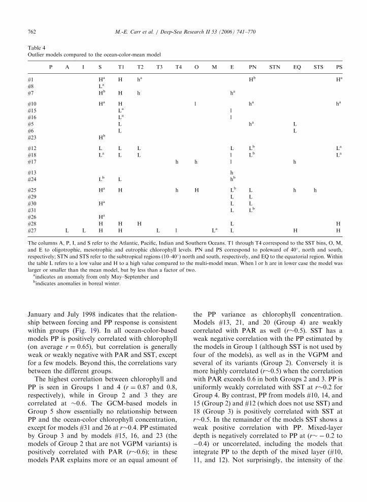
Outlier models compared to the ocean-color-mean model
P A I S T1 T2 T3 T4 O M E PN STN EQ STS PS
#1 Ha H ha Hb Ha
#8 La
#7 Hb H h ha
#10 Ha H l ha ha
#15 La l
#16 La l
#5 L ha L
#6 L L
#23 Hb
#12 L L L L Lb La
#18 La L L l Lb La
#17 h h l h
#13 h
#24 Lb L hb
#25 Ha H h H Lb L h h
#29 L L
#30 Ha L L
#31 L Lb
#26 Ha
#28 H H H L H
#27 L L H H L l La L H H
The columns A, P, I, and S refer to the Atlantic, Pacific, Indian and Southern Oceans. T1 through T4 correspond to the SST bins, O, M,
and E to oligotrophic, mesotrophic and eutrophic chlorophyll levels. PN and PS correspond to poleward of 40�, north and south,
respectively; STN and STS refer to the subtropical regions (10–40�) north and south, respectively, and EQ to the equatorial region. Within
the table L refers to a low value and H to a high value compared to the multi-model mean. When l or h are in lower case the model was
larger or smaller than the mean model, but by less than a factor of two.aindicates an anomaly from only May–September andbindicates anomalies in boreal winter.
M.-E. Carr et al. / Deep-Sea Research II 53 (2006) 741–770762
January and July 1998 indicates that the relation-ship between forcing and PP response is consistentwithin groups (Fig. 19). In all ocean-color-basedmodels PP is positively correlated with chlorophyll(on average r ¼ 0:65), but correlation is generallyweak or weakly negative with PAR and SST, exceptfor a few models. Beyond this, the correlations varybetween the different groups.
The highest correlation between chlorophyll andPP is seen in Groups 1 and 4 (r ¼ 0:87 and 0.8,respectively), while in Group 2 and 3 they arecorrelated at �0.6. The GCM-based models inGroup 5 show essentially no relationship betweenPP and the ocean-color chlorophyll concentration,except for models #31 and 26 at r�0:4. PP estimatedby Group 3 and by models #15, 16, and 23 (themodels of Group 2 that are not VGPM variants) ispositively correlated with PAR (r�0:6); in thesemodels PAR explains more or an equal amount of
the PP variance as chlorophyll concentration.Models #13, 21, and 20 (Group 4) are weaklycorrelated with PAR as well (r�0:5). SST has aweak negative correlation with the PP estimated bythe models in Group 1 (although SST is not used byfour of the models), as well as in the VGPM andseveral of its variants (Group 2). Conversely it ismore highly correlated (r�0:5) when the correlationwith PAR exceeds 0.6 in both Groups 2 and 3. PP isuniformly weakly correlated with SST at r�0:2 forGroup 4. By contrast, PP from models #10, 14, and15 (Group 2) and #12 (which does not use SST) and18 (Group 3) is positively correlated with SST atr�0:5. In the remainder of the models SST shows aweak positive correlation with PP. Mixed-layerdepth is negatively correlated to PP at (r�� 0:2 to�0:4) or uncorrelated, including the models thatintegrate PP to the depth of the mixed layer (#10,11, and 12). Not surprisingly, the intensity of the
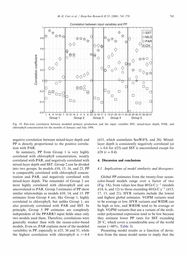
ARTICLE IN PRESS
1 8 9 14 22 7 10 15 16 2 4 5 6 23 12 18 17 3 13 21 20 19 11 24 25 29 30 31 26 28 27-0.6
-0.4
-0.2
0
0.2
0.4
0.6
0.8
1
SSTMLDPARChl
Correlation between input variables and PP
Cor
rela
tion
coef
ficie
nt
Group 1 Group 2 Group 3 Group 4 Group 5
Fig. 19. Pair-wise correlation between modeled primary production and the input variables SST, mixed-layer depth, PAR, and
chlorophyll concentration for the months of January and July 1998.
M.-E. Carr et al. / Deep-Sea Research II 53 (2006) 741–770 763
negative correlation between mixed-layer depth andPP is directly proportional to the positive correla-tion with PAR.
In summary, PP from Group 1 is very highlycorrelated with chlorophyll concentration, weaklycorrelated with PAR, and negatively correlated withmixed-layer depth and SST. Group 2 can be dividedinto two groups. In models #10, 15, 16, and 23, PPis comparably correlated with chlorophyll concen-tration and PAR, and negatively correlated withmixed-layer depth. The remainder of Group 2 aremost highly correlated with chlorophyll and areuncorrelated to PAR. Group 3 estimates of PP showsimilar relationships as models #10, 14, and 15. PPestimates from Group 4 are, like Group 1, highlycorrelated to chlorophyll, but unlike Group 1, arealso positively correlated with PAR and SST. Inprinciple, Group 5 PP estimates are completelyindependent of the PPARR3 input fields since onlytwo models used them. Therefore, correlations weregenerally weaker than with the ocean-color-basedmodels. Even so, PAR explains most of the modeledvariability in PP, especially in #25, 30 and 31, whilethe highest correlation with chlorophyll is r�0:4
(#31, which assimilates SeaWiFS, and 26). Mixed-layer depth is consistently negatively correlated (atr ¼ 0:6 for #25) and SST is uncorrelated except for#28 (r ¼ 0:4).
4. Discussion and conclusions
4.1. Implications of model similarity and divergence
Global PP estimates from the twenty-four ocean-color-based models range over a factor of two(Fig. 5A), from values less than 40GtC y�1 (models#14, 6, and 12) to those exceeding 60GtC y�1 (#15,17, 13, and 21). HYR variants include the lowestand highest global estimates. VGPM variants tendto be average or low, HYR variants and WIDR canbe high or low, and WRDR tend to be average orhigh. VGPM variants that use a variant of the sixth-order polynomial expression tend to be low becausethey estimate lower PP rates for SST exceeding20 �C, which cover a considerable area of the worldocean (�60%, Table 3).
Presenting model results as a function of devia-tion from the mean model seems to imply that the

ARTICLE IN PRESSM.-E. Carr et al. / Deep-Sea Research II 53 (2006) 741–770764
mean is inherently better. We do not believe this tobe the case; there is no way to quantify modelperformance without comparing the output to insitu data (part 3, Friedrichs et al., in preparation).We propose instead that the conditions or regionsfor which the models differ are those for which it ismore difficult to model photosynthesis. For exam-ple, model output converges more in regions whichhave provided more data for model development(Fig. 7, Table 4) and those which do not presentHNLC conditions. The most difficult regions arepoleward of 40� in all basins, the equatorial region,and northern subtropical Indian Ocean. This resultsfrom differences in model output for high chlor-ophyll concentrations and for extreme SST values(o10 �C and 420 �C).
The Southern Ocean is unquestionably the mostchallenging large basin. Two models and a variant(#8/9 and 24) were formulated for the SouthernOcean and parameterized solely with SouthernOcean data. PP estimated by models #8 and 24 islower than that of the mean model (Fig. 7).However, PP from model #9, which aims to correctthe chlorophyll determination in this region, and#19, which also included Southern Ocean data in itsformulation and parameterization, are 20–50%larger than the mean (Fig. 7).
The model anomalies are summarized in Table 4.Anomalous models in Group 1 tend to overestimatePP in the Southern Ocean, and under low tempera-ture and high chlorophyll conditions. Group 1generally produces low PP (except for eutrophicconditions, Figs. 8 and 9) and is highly correlated tothe chlorophyll fields (Fig. 19). Group 2 estimates ofPP tend to be higher than average; the anomalousmodels generally overestimate PP in the SouthernOcean, while underestimating PP for SSTo0 �C and overestimating it for 10 �C4SSTo20 �Cand in mesotrophic waters (Table 4, Figs. 8 and 10).This group includes the standard VGPM and mostvariants for which maximum photosynthetic ratesoccur at or below 20 �C (Fig. 18). PP estimated byfour of the models in this group (#10, 15, 16, and 23,a WIDI, two WIDR and a WRDR) is morecorrelated to PAR than to chlorophyll, while theremaining four are correlated only to chlorophyllconcentration (Fig. 19). PP estimated by Group 3tends to be low, except for model #17 (Fig. 5).Group 3 models are quite anomalous compared tothe mean, with a tendency to underestimate PP inthe Southern Ocean and under conditions of lowtemperature (o10 �C), and to overestimate PP in
the equatorial region (Table 4). The group averagemodel is generally low compared to the mean exceptin oligotrophic waters (Figs. 6, 8, and 10). Thesemodels are more or equally correlated to PAR thanto chlorophyll (Fig. 19). Models in Group 4 tendto overestimate PP compared to the mean model(Fig. 5). PP is high particularly in mesotrophic andoligotrophic waters and for SST exceeding 20 �C.All of these models include an exponential functionof SST (Fig. 15). The global PP fields are highlycorrelated with chlorophyll concentration and, insome cases with PAR and, unlike in Group 1,positively if weakly correlated with SST (Fig. 19).
Finally, Group 5 estimates of PP were comparableto those of the ocean-color-based models (Fig. 5).They tend to overestimate PP in the SouthernOcean, in the equatorial region, and at SST lessthan 10 �C and over 20 �C, and to underestimatehigh chlorophyll concentrations (Table 4). TheGCM-based model fields are weakly related to theinput fields, except for #25, 30, and 31, which arecorrelated with PAR at rX0:6, and #25, which isnegatively correlated with mixed-layer depth(r ¼ �0:6; Fig. 19). Some of the GCM-basedmodels restore nutrients to climatology at depth,which in some comparison studies can increaseglobal production by �10GtC y�1.
Not surprisingly, the parameterization of themaximum or optimal photosynthetic rate has largeimpact on the variability of the ocean-color-basedmodels and consequently on the relationshipgroups. Specifically the results of the sensitivityanalysis show that the sensitivity to SST perturba-tions, regardless of model complexity, helps explainthe observed dendrogram (Figs. 16 and 4). The largedivergence in response to SST perturbations illus-trates the need to improve our understanding, andability to model, the effect of temperature onphotosynthesis.
4.2. Strategy for model improvement
Ocean-color-based modeling of primary produc-tion is an active area of research, and new modelsare under development. Ongoing efforts strive toinclude more data, from a broader geographic rangeand for more diverse conditions, and to improvemodel formulation and parameterization. Globalestimation of primary production from ocean colorrequires extrapolating sparse point measurements.Aspects of the photosynthetic process and of theenvironmental conditions (e.g., light or nutrients)
ARTICLE IN PRESSM.-E. Carr et al. / Deep-Sea Research II 53 (2006) 741–770 765
are parameterized as a function of either biogeo-graphy and/or one or more variables which can bemeasured from spaceborne sensors. The problem isdata limited by the amount of (1) representative insitu measurements and (2) satellite-accessible in-formation. Strategies which combine remotely-sensed variables with historical or modeled informa-tion that can be linked to geography, biome, orregime are compelling as they hopefully include thebest of both worlds.
Complex models are computer-intensive althoughshortcuts can be made via look-up tables or usingsimplifying assumptions. The advantage of complexmodels is that the photosynthetic process isrepresented with greater fidelity and detail, whichallows for greater subtlety in the forcing fields. Asmore in situ data, or improved satellite data (such asinformation on nutrient fields, phytoplankton sizeclass or functional groups, or photoadaptive state),become available they can be exploited within mostof the existing complex formulations.
The advantage of simple models is that they arevery easily implemented. The simplest modelexamined (#1), a simple function of chlorophyllconcentration, estimates consistent global andregional averages production (Fig. 5A). However,this model cannot reflect temporal or spatialvariability that does not impact the chlorophyllconcentration, including for example, the absence oflight. Seasonal variability is underestimated com-pared to the other models (best seen in Fig. 13) andinterannual variability is also less than average(Fig. 5B). Model #1 also overestimates PP inconditions of low PAR or very low SST, andconsequently at high latitudes (Figs. 7, 11, and 13).Models that incorporate PAR or SST generateseasonal and temporal variability that is indistin-guishable from that of complex models. However,simple parameterizations are more likely to bebiased by the data used in the formulation.Competing processes, such as for example thephotosynthetic response to temperature versus thecorrelation between temperature and nutrient con-tent, can easily be confounded or canceled out,especially when limited input data are available toparameterize the processes.
Ocean-color-based models need to resolve varia-bility in addition to average values. Siegel et al.(2001) compared ten PP models (of varied complex-ity, including WRDR) with a six-year time series ofPP and bio-optical measurements at the subtropicalBermuda Atlantic Time Series (BATS) site. PP
models explained �30% of the observed variance.The best models in reproducing the mean wereunable to capture the variability. They concludedthat the assumptions of steady state and balancedgrowth inherent to bio-optical PP models cannotreproduce the unsteady disturbed environment ofcells in the ocean.
When asked what is needed to improve modelperformance, all model developers coincide inrequesting more data, ideally together with ancillarydata such as nutrients and community structure. Animproved understanding of the photosyntheticprocess requires measurement of the photosyntheticparameters in addition to that of primary produc-tion. Data are especially limited from the SouthernOcean, the subtropics, HNLC regions, and thecoastal ocean. Initial results for the equatorialPacific indicate that the community models areimproving compared to PPARR2: mismatch with insitu data on the equator decreased by over a factorof two (Friedrichs et al., in prep). Specific concernsfor future progress include improved formulation ofthe quantum yield and of the light field, and moredata on the vertical distribution of chlorophyll.Comparisons with in situ data invariably bring upthe limitations of discrete 14C uptake measurements(e.g., Richardson et al., 1984). Our strategy is basedon 14C measurements because of data density, butthought should be placed on the use of alternateestimates of photosynthetic rate, such as oxygenproduction (e.g., Bender et al., 2000).
As in PPARR1/2, the PPARR3 modeling exerciseincludes comparison with in situ data, necessary toquantify model performance (Friedrichs et al., inprep). Parts 1 and 2 presented here provide anunprecedented understanding of the observed simi-larity among the models and of the conditions underwhich they perform differently. The large number ofparticipating ocean color and GCM-based modelsprovides an expanded perspective on the range ofmodel performance. We have found that the form inwhich SST is used impacts the relationship betweenmodel output. Future plans include a more com-prehensive in situ comparison, including coastalregions, the Southern Ocean, Arabian Sea, and amore detailed examination of temporal variabilityin subtropical regions (i.e. the Bermuda and Hawaiitime series stations). As in PPARR3, we anticipatemodel development and refinement, and hope toperform ongoing comparison of model perfor-mance, such as shown here, independently of thein situ data.
ARTICLE IN PRESSM.-E. Carr et al. / Deep-Sea Research II 53 (2006) 741–770766
Acknowledgments
We thank Tony Lee of JPL and Stephen Yeagerand Scott Doney (now at WHOI) of NCAR forgenerously providing modeled fields of mixed-layerdepth. We are grateful to the SeaWiFS ScienceProject for the SeaWiFS data set and to the NOAA/NASA AVHRR Pathfinder project for SST, madeavailable by the JPL-PODAAC. We thank twoanonymous reviewers for helpful comments thatimproved an earlier version. Funding was providedby the NASA Ocean Biogeochemistry Programwithin the Carbon Cycle Science Program. Theresearch described in this paper was carried out atthe Jet Propulsion Laboratory, California Instituteof Technology, under a contract with the NationalAeronautics and Space Administration.
Appendix
Model #1: This model estimates PP asffiffiffiffiffiffiffichlp
(Eppley et al., 1985). It ignores any external forcingor changes in physiological state. While othermodels introduce complexity from geography orforcing fields, this model assumes that the standingstock is sole determinant of photosynthetic rate. Allbiomass performs identically.
Models #2/3/4: The vertically generalized produc-tion model (VGPM) developed by Behrenfeld andFalkowski (1997a) is one of the most widely knownand used WIDI PP models. The maximum observedphotosynthetic rate within the water column, PB
opt, isobtained as a seventh-order polynomial of SST.Companion model #3 only differs from #2 in thatPBopt is estimated as an exponential function of
temperature following Eppley (1972). Model #4 isidentical to Model #2, but was run independently asa former standard MODIS PP product.
Model #5: This VGPM variant estimates the totalintegrated chlorophyll concentration from a con-tinuous function (Morel and Berthon, 1989) ratherthan in two steps as in Model #2; the euphotic depth(attenuation coefficient) is defined following Moreland Maritorena (2001).
Model #6: This VGPM variant formulates PBopt as
a function of SST and chlorophyll concentration(Kameda and Ishizaka,, in press). The model isbased on the assumptions that changes in chlor-ophyll concentration depend on the abundance oflarge phytoplankton and that chlorophyll-specificproductivity is inversely proportional to phyto-plankton size.
Model #7: This VGPM defines PBopt by multi-
plying a theoretical maximum PBopt by nutrient and
light limitation factors obtained from a globally-runecosystem model (Moore et al., 2002ba). It assumesthat PB
opt depends more on available nutrients andlight than on SST.
Models #8/9: This VGPM variant was developedfor the Southern Ocean and was only run south of50 �S (Dierssen and Smith, 2000; Dierssen et al.,2000). It uses the average PB
opt measured in the studyarea, as no relationship was found between envir-onmental observations and PB
opt. Model #8 uses thestandard chlorophyll concentration as input. #9answers the challenges to satellite determination ofchlorophyll in the Southern Ocean by transformingthe SeaWiFS value with an empirical relationshipobserved between ocean color and in situ measure-ments.
Model #10: This model is based on the formula-tion obtained through dimensional analysis by Plattand Sathyendranath (1993). The photosyntheticparameters (PB
max and the photo-acclimation para-meter Ek) are assigned by combining a temperature-dependent relationship for the maximum growthrate (Eppley, 1972) with dynamic provinces derivedfrom fuzzy logic (as in Moore et al., 2001) toretrieve the carbon to chlorophyll ratio followingthe empirical relation of Cloern et al. (1995).Primary production is integrated to the mixed-layerdepth.
Model #11: This model is the standard Howard,Yoder, Ryan (HYR) model (Howard and Yoder,1997). Maximum growth rate is parameterized as afunction of SST according to Eppley (1972).Primary production is integrated to the mixed-layerdepth rather than to the euphotic depth.
Model #12: This HYR variant uses mixed-layerdepth information to quantify the photoadaptivevariables within the euphotic zone, as well as toaddress water column partitioning of primaryproduction relative to euphotic depth.
Model #13: This HYR variant integrates photo-synthesis to the euphotic depth as defined inBehrenfeld and Falkowski (1997a) rather than tothe mixed-layer depth (Carr, 2002).
Model #14: This model uses an artificial neuralnetwork to perform a generalized nonlinear regres-sion of PP on several predictive variables,includinglatitude, longitude, day length, mixed-layer depth,SST, PB
opt (computed according to the VGPM),PAR, and surface chlorophyll (Scardi, 2000, 2001).Since there are insufficient data to calibrate the

ARTICLE IN PRESSM.-E. Carr et al. / Deep-Sea Research II 53 (2006) 741–770 767
neural network on a global scale, PP values fromother models (VGPM, HYR, and the MOD-27formulation (Esaias, 1996)) were considered mea-surements where there were none.
Models #15/16/17: These three models are WIDRmodels. Model #14 uses Behrenfeld and Falkowski(1997a) to estimate PB
opt. The surface spectralirradiance, estimated with Gregg and Carder(1990), is used to obtain a spectrally weighteddepth-averaged light attenuation coefficient withinthe mixed layer. Surface irradiance is convertedfrom cosine to scalar. Companion model #15, incontrast, does not convert the irradiance fromcosine to scalar. Model #16 differs from #14 byusing the PB
max function from Antoine and Morel(1996).
Model #18: This WIDR model estimates depth-dependent photosynthesis as a function of chlor-ophyll concentration, temperature, and PAR. Thedepth-distribution of PAR is determined by surfacechlorophyll concentration while the depth-distribu-tion of chlorophyll is given by the PAR profile andthe surface chlorophyll concentration. The carbonfixation rate is empirically estimated as a function ofPAR and temperature (Asanuma et al., 2003).
Model #19: This WIDR model is based onchlorophyll-specific phytoplankton absorption,which is parameterized empirically as a function ofSST (Marra et al., 2003). Absorption by photosyn-thetic pigments is distinguished from total absorp-tion; the former is used to calculate productivity andthe latter is used to estimate light attenuation in thewater column. The quantum efficiency is obtainedfrom a hyperbolic tangent and a constant fmax. Thedepth profile of chlorophyll is estimated assuming agaussian shape with parameters determined by thesurface value. The attenuation coefficient of chlor-ophyll is also SST-dependent.
Model #20: This WRDR model (Morel, 1991) isbased on measurements of photosynthesis versusirradiance and is formulated using chlorophyll-specific wavelength-resolved absorption and quan-tum yield. Temperature dependence is given by theparameterization of PB
max which follows Eppley(1972). The chlorophyll profile is determined to bewell-mixed or stratified according to the ratio ofmixed-layer depth and the euphotic depth, and ifstratified, assigned a gaussian profile as in Moreland Berthon (1989). Mean photo-physiologicalparameters are from Morel et al. (1996). The modelis run in its ‘satellite’ version (Antoine et al., 1996),where PP is the product of integral biomass, the
daily irradiance, and c� (the cross-section of algaefor photosynthesis per unit of areal chlorophyllbiomass). Lookup tables for c� were previouslygenerated using the full WRDR model, and are usedto increase computational efficiency.
Model #21: This model is an implementation ofthe Morel (1991) WRDR model in which the depthdistribution of chlorophyll is assumed constantthroughout the water column. The broadbandincident PAR is spectrally resolved using a look-up-table generated from a single run of the Greggand Carder (1990) marine irradiance model wherethe effects of clouds and aerosols are essentiallylinearly scaled. The model uses 60-min time and10-m depth steps at 5-nm wavelength resolutionwhen run using the global datasets.
Model #22: This WRDR follows the model ofPlatt and Sathyendranath (1988) as implemented atglobal scale by Longhurst et al. (1995). It usesbiogeographical provinces to define the values of theparameters to describe the light-photosynthesiscurve and the chlorophyll depth profile. Photosyn-thetic parameters were updated using an extendeddata set provided by the Bedford Institute ofOceanography and an extensive literature review.Spectral surface irradiance is first estimated inde-pendently with the model of Gregg and Carder(1990) combined with a correction for cloud coverand then scaled to match the PAR values providedfor the exercise. Spectral light is subsequentlypropagated in the water column with a bio-opticalmodel with updated parameterizations of theinherent optical properties. All changes to theoriginal implementation of Longhurst et al. (1995)are detailed by Melin (2003).
Model #23: This WRDR model derives spectralirradiance from the PAR using Tanre et al. (1990).Quantum yield is parameterized from a maximumvalue and a light dependent term (Waters et al.,1994; Bidigare et al., 1992). The chlorophyll profileis assumed vertically uniform. A sigmoidal tem-perature dependence was applied to the maximumquantum yield, based on a vertical profile oftemperature derived from SST and mixed-layerdepth.
Model #24: This WRDR was developed for theSouthern Ocean (Arrigo et al., 1998), but has beenapplied to the global fields in this study. It is basedon spectrally varying chlorophyll absorption and ascaling of the photo-acclimation parameter Ek tothe daily mean irradiance. The rate of production isdetermined by temperature and by light limitation.

ARTICLE IN PRESSM.-E. Carr et al. / Deep-Sea Research II 53 (2006) 741–770768
Chlorophyll is assumed uniform in the mixed layerand decreases exponentially at greater depths.
Model #25: The Pelagic Interactions Scheme forCarbon and Ecosystem Studies (PISCES) oceanbiogeochemistry model has three nutrients (Fe, P,and Si), and two size classes each of phytoplanktonand zooplankton, as well as detritus and semi-labiledissolved organic matter (Aumont et al., 2003; Boppet al., 2003). PISCES is coupled online to the OPAgeneral circulation model (Madec et al., 1998). OPAhas a horizontal resolution of 2�; the latitudinalresolution is enhanced to 0.5� at the equator andthe pole. It resolves 30 vertical levels at 10-mintervals in the top 100m. It is forced with dailyaveraged values of winds and fluxes from theNational Centers for Environmental Prediction(NCEP) reanalysis.
Model #26: This ecosystem model (Moore et al.,2002a,b) has four nutrients (nitrogen, phosphorus,silicon, and iron) and three phytoplankton groups(diatoms, diazotrophs, and a generic small phyto-plankton class). Growth rates can be limited byavailable nutrients and/or light levels. The diatomscan also be limited by silicon and the diazotrophsare not nitrogen-limited. This model is run asmultiple 1-D mixed layer models, forced here bythe provided mixed-layer depth.
Model #27: This 11-compartment North PacificEcosystem Model Used for Regional Oceanography(NEMURO), developed by the North PacificMarine Science Organization (Eslinger et al.,2000), has two size classes each of phytoplanktonand zooplankton, and two nutrients: nitrate andsilicate. The coupled GCM and ecosystem model isdescribed by Aita et al. (2003). The horizontalresolution is 1 by 1� over a global domain notincluding the Arctic Ocean.
Model #28: This biogeochemical model estimatesnew production by restoring surface nitrate to themonthly World Ocean Atlas 2001 data synthesis(http://www.nodc.noaa.gov/OC5/WOA01/pr-woa01.html) and then applies a spatially dependent f-ratioto obtain primary production. Climatological forcingwas used.
Model #29: This PISCES model variant, PISCES-T, has improved parameterization of meso-zoo-plankton growth and mortality rates, and atemperature-dependent degradation of particulateorganic matter (Buitenhuis et al., 2006). As in #25, itis coupled to the OPA and is forced by NCEPreanalysis. This model version does not restore toclimatological nutrients below the mixed layer.
Model #30: The NASA Ocean BiogeochemicalModel (NOBM) simulates four phytoplanktongroups (diatoms, chlorophytes, cyanobacteria, andcoccolithophores) and four nutrients (nitrate, am-monium, silica, and iron) (Gregg et al., 2003). Themodel is approximately 0.8� resolution with 14vertical layers in quasi-isopycnal configuration.The model was forced by monthly mean windsand shortwave radiation from NCEP for 1998 and1999.
Model #31: In this NOBM variant SeaWiFSchlorophyll data were assimilated for 1998 and1999. Assimilation occurred on a daily basis, usingthe Conditional Relaxation Analysis Method (Oort,1983). The assimilation affected the model repre-sentations of total chlorophyll (sum of the fourphytoplankton groups), but not the individualcommunity distributions directly. Primary produc-tion was affected by the change in total chlorophyll,as well as by indirect effects such as subsurfaceirradiance resulting from absorption and scatteringby the changed chlorophyll field.
References
Aita, M.N., Yamanaka, Y., Kishi, M.J., 2003. Effect of
ontogenetic vertical migration of zooplankton on the results
of NEMURO embedded in a general circulation model.
Fisheries Oceanography 12, 284–290.
Antoine, D., Morel, A., 1996. Oceanic primary production 2.
Adaptation of a spectral light-photosynthesis model in view
of application to satellite chlorophyll observations. Global
Biogeochemical Cycles 10, 43–55.
Antoine, D., Andre, J.-M., Morel, A., 1996. Oceanic primary
production 2. Estimation at global scale from satellite
(Coastal Zone Color Scanner) chlorophyll. Global Biogeo-
chemical Cycles 10, 57–69.
Arrigo, K.R., Worthern, D., Schnell, A., Lizotte, M.P., 1998.
Primary production in Southern Ocean waters. Journal of
Geophysical Research 103, 15587–15600.
Asanuma, I., Nieke, J., Matsumoto, K., Kawano, T., 2003.
Optical properties control primary productivity model on the
East China Sea. In: Frouin, J.R. (Ed.), Ocean Remote Sensing
and Applications, vol. 4892. SPIE, pp. 312–319.
Aumont, O., Maier-Reimer, E., Blain, S., Pondaven, P., 2003. An
ecosystem model of the global ocean including Fe, Si, P co-
limitations. Global Biogeochemical Cycles 17, doi:10.1029/
2001GB001745.
Behrenfeld, M., Falkowski, P., 1997a. Photosynthetic rates
derived from satellite-based chlorophyll concentration. Lim-
nology and Oceanography 42 (1), 1–20.
Behrenfeld, M., Falkowski, P., 1997b. A consumer’s guide to
phytoplankton primary productivity models. Limnology and
Oceanography 42 (7), 1479–1491.
Bender, M., Dickson, M.-L., Orchardo, J., 2000. Net and gross
production in the Ross Sea as determined by incubation
ARTICLE IN PRESSM.-E. Carr et al. / Deep-Sea Research II 53 (2006) 741–770 769
experiments and dissolved O2 studies. Deep Sea Research II
47, 3141–3158.
Berger, W.H., 1989. Global maps of primary productivity. In:
Berger, W.H., Smetacek, V.S., Wefer, G. (Eds.), Productivity
of the Ocean: Present and Past. Wiley, Berlin, pp. 429–455.
Bidigare, R.R., Prezelin, B.B., Smith, R.C, 1992. Bio-optical
models and the problems of scaling. In: Primary Productivity
and Biogeochemical Cycles in the Sea. Plenum Press,
New York, pp. 175–212.
Bopp, L., Kohfeld, K., Le Quere, C, Aumont, O., 2003. Dust
impact on marine biota and atmospheric CO2 during glacial
periods. Paleoceanography 18, 10.1029/2002PA000810.
Buitenhuis, E.T., Le Quere, C., Aumont, O., Beaugrand, G.,
Bunker, A., Hirst, A., Ikeda, T., O’Brien, T., Piontkovski, S.,
Straile, D., 2006. Biogeochemical fluxes through mesozoo-
plankton. Global Biogeochemical Cycles 20 (2), GB2003.
Campbell, J., Antoine, D., Armstrong, R., Balch, W., Barber, R.,
Beherenfeld, M., Bidigare, R., Bishop, J., Carr, M.-E., Esaias,
W., Falkowski, P., Hoepffner, N., Iverson, R., Kiefer, D.,
Lohrenz, S., Marr, J., Morel, A., Ryan, J., Vedernikov, V.,
Waters, K., Yentsch, C, Yoder, J., 2002. Comparison of
algorithms for estimating ocean primary production from
surface chlorophyll, temperature, and irradiance. Global
Biogeochemical Cycles 16(3), 10.1029/2002GL015068.
Carr, M.-E., 2002. Estimation of potential productivity in
Eastern Boundary Currents using remote sensing. Deep-Sea
Research II 49, 59–80.
Cloern, J.E., Grenz, C., Vidergar-Lucas, L., 1995. An empirical
model of the phytoplankton chlorophyllicarbon ratio—the
conversion factor between productivity and growth rate.
Limnology and Oceanography 40, 1313–1321.
Dierssen, H., Smith, R.C., 2000. Bio-optical properties and
remote sensing ocean color algorithms for Antarctic Peninsu-
la waters. Journal of Geophysical Research 105 (C),
26301–26312.
Dierssen, H., Vernet, M., Smith, R.C., 2000. Optimizing models
for remotely estimating primary production in Antarctic
coastal waters. Antarctic Science 12, 20–32.
Eppley, R.W., 1972. Temperature and phytoplankton growth in
the sea. Fisheries Bulletin 70, 1063–1085.
Eppley, R., Steward, E., Abbott, M., Heyman, U., 1985.
Estimating ocean primary production from satellite chlor-
ophyll: introduction to regional differences and statistics for
the Southern California Bight. Journal of Plankton Research
7, 57–70.
Esaias, W., 1996. MODIS algorithm theoretical basis document
for product MOD-27: ocean primary productivity. WWW
Page hhttp://modis.gsfc.nasa.gov/data/atbd/atbd-mod24.pdfi.
Eslinger, D.V., Kashiwai, M.B., Kishi, M.J., Megrey, B.A.,
Ware, D.M., Werner, F.E., 2000. Final report of the
international workshop to develop a prototype lower trophic
level ecosystem model for comparison of different marine
ecosystems in the north Pacific. PICES Scientific Report 15,
1–77.
Field, C., Behrenfeld, M., Randerson, J., Falkowski, P., 1998.
Primary production of the biosphere: integrating terrestrial
and oceanic components. Science 281 (5374), 237–240.
Friedrichs, M.A.M., Carr, M.-E., Barber, R., Schmeltz, M.,
Gentili, B., Morel, A., Arrigo, K.R., Reddy, T., Asanuma, I.,
Behrenfeld, M., Bidigare, B., Ciotti, A., Dierssen, H., Dowell,
M., Dunne, J., Esaias, W., Turpie, K., Hoepffner, N., Melin,
F., Ishizaka, J., Le Quere, C., Aumont, O., Marra, J., Moore,
K., Ryan, J., Scardi, M., Smyth, T., Groom, S., Tilstone,
G.H., Waters, K., Yamanaka, Y., in preparation. Compar-
ison of primary production estimates in the tropical Pacific
Ocean, in preparation.
Gregg, W., Carder, K., 1990. A simple spectral solar irradiance
model for cloudless maritime atmospheres. Limnology and
Oceanography 35, 1657–1675.
Gregg, W.W., Ginoux, P., Schopf, P., Casey, N., 2003.
Phytoplankton and iron: validation of a global three-
dimensional ocean biogeochemical model. Deep-Sea Research
II 50, 3143–3169.
Howard, K.L., Yoder, J.A., 1997. Contribution of the sub-
tropical oceans to global primary production. In: Liu, C.-T.
(Ed.), Space Remote Sensing of Subtropical Oceans. vol.
COSPAR Colloquia Series, vol. 8. Proceedings of COSPAR
Colloquium on Space Remote Sensing of Subtropical Oceans,
Taiwan. Pergamon, New York, pp. 157–168.
Kameda, T., Ishizaka, J., in press. Size-fractionated primary
production estimated by a two-phytoplankton community
model applicable to ocean color remote sensing. Journal of
Oceanography, in press.
Koblentz-Mishke, O.I., Volkovinsky, V.V., Kabanova, Y.G.,
1970. Plankton primary production of the world ocean.
In: Wooster, W. (Ed.), Scientific Exploration of the
South Pacific. National Academy of Sciences, Washington,
DC, pp. 183–193.
Le Borgne, R., Barber, R., Delcroix, T., Inoue, H., Mackey, D.,
Rodier, M., 2002. Pacific warm pool and divergence: temporal
and zonal variations on the equator and their effects on
the biological pump. Deep-Sea Research 49 (13–14),
2471–2512.
Longhurst, A., Sathyendranath, S., Piatt, T., Caverhill, C., 1995.
An estimate of global primary production in the ocean from
satellite radiometer data. Journal of Plankton Research 17,
1245–1271.
Madec, G., Delecluse, P., Imbard, M., Levy, C., 1998. OPA 8.1.
Ocean General Circulation Model Reference Manual. IPSL
Notes du pole de modelisation, Note 11.
Marra, J., Ho, C., Trees, C., 2003. An alternative algorithm for
the calculation of primary productivity from remote sensing
data. LDEO Technical Report #LDEO-2003-1.
McClain, C.R., Cleave, M.L., Feldman, G., Gregg, W., Hooker,
S., Kuring, N., 1998. Science quality SeaWiFS data for global
biosphere research. Sea Technology 39, 10–16.
Melin, F., 2003. Potentiel de la teledetection pour l’analyse des
proprietes optiques du systeme ocean-atmosphere et applica-
tion a l’estimation de la photosynthese phytoplanctonique.
Ph.D., Universite Paul Sabatier, Toulouse, France, unpub-
lished.
Middleton, G.V., 2000. Data Analysis in the Earth Sciences
Using MATLAB. Prentice-Hall, Englewood Cliffs, NJ.
Moore, J.K., Doney, S.C., Glover, D.M., Fung, I.Y., 2002a. Iron
cycling and nutrient-limitation patterns in surface waters of
the world ocean. Deep-Sea Research II 49, 463–507.
Moore, J.K., Doney, S.C., Kleypas, J.A., Glover, D.M., Fung,
I.Y., 2002b. An intermediate complexity marine ecosystem
model for the global domain. Deep-Sea Research II 49,
403–462.
Moore, T.S., Campbell, J., Feng, H., 2001. A fuzzy logic
classification scheme for selecting and blending satellite ocean
color algorithms. IEEE Transactions on Geoscience and
Remote sensing 39 (8), 1764–1776.

ARTICLE IN PRESSM.-E. Carr et al. / Deep-Sea Research II 53 (2006) 741–770770
Morel, A., 1991. Light and marine photosynthesis: a spectral
model with geochemical and climatological implications.
Progress in Oceanography 26, 263–306.
Morel, A., Berthon, J.F., 1989. Surface pigments, algal biomass
profiles, and potential production of the euphotic layer:
relationships reinvestigated in view of remote-sensing applica-
tions. Limnology and Oceanography 34 (8), 1545–1562.
Morel, A., Antoine, D., Babin, M., Dandonneau, Y., 1996.
Measured and modeled primary production in the northeast
Atlantic (EUMELI JGOFS program): the impact of natural
variations in photosynthetic parameters on model predictive
skill. Deep-Sea Research I 43, 1273–1304.
Morel, A., Maritorena, S., 2001. Bio-optical properties of oceanic
waters: A reappraisal. Journal of Geophysical Research 106,
7163–7180.
Ondrusek, M.E., Bidigare, R.R., Waters, K., Karl, D.M., 2001. A
predictive model for estimating rates of primary production in
the subtropical north Pacific Ocean. Deep-Sea Research II 48
(8–9), 1837–1863.
Oort, A.H., 1983. Global atmospheric circulation statistics,
1958–1973. NOAA Professional Paper 14.
Platt, T., Sathyendranath, S., 1988. Oceanic primary production:
estimation by remote sensing at local and regional scales.
Science 241, 1613–1620.
Platt, T., Sathyendranath, S., 1993. Estimators of pri-
mary production for interpretation of remotely sensed data
on ocean color. Journal of Geophysical Research 98,
14561–14567.
Richardson, K., Samelsson, G., Hallgren, J., 1984. The relation-
ship between photosynthesis measured by C-14 incorporation
and by uptake of inorganic carbon in unicellular algae.
Journal of Experimental Marine Biology and Ecology 81
(3), 241–250.
Rohlf, F.J., 1963. Classification of Aedes by numerical taxonomic
methods (Diptera: Culicidae). Annals of the Entomological
Society of America 56, 798–804.
Scardi, M., 2000. Neuronal network models of phytoplankton
primary production. In: Lek, S.G.J.-F. (Ed.), Artificial
Neuronal Networks: Application to Ecology and Evolution.
Springer, Berlin/Heidelberg, pp. 115–129.
Scardi, M., 2001. Advances in neural network modeling of
phytoplankton primary production. Ecological Modelling
146, 33–45.
Siegel, D., Westberry, T., O’Brien, M., Nelson, N., Michaels, A.,
Morrison, J., Scott, A., Caporelli, E., Sorensen, J., Maritor-
ena, S., Garver, S., Brody, E., Ubante, J., Hammer, M., 2001.
Bio-optical modeling of primary production on regional
scales: the Bermuda BioOptics project. Deep-Sea Research
II 48, 1865–1896.
Tanre, D., Deroo, C., Duhaut, P., Herman, M., Morcrett, J.,
Perbos, J., Deschamps, P., 1990. Description of a computer
code to simulate the satellite signal in the solar spectrum.
International Journal of Remote Sensing 11, 659–668.
Waters, K., Smith, R., Marra, J., 1994. Phytoplankton produc-
tion in the Sargasso Sea as determined using optical mooring
data. Journal of Geophysical Research 99, 18385–18402.