A comparison of four methods for projecting households

international Journal of Forecasting 8 (1992) 509-527

North-t~~~lland

509

A comparison of four methods for projecting households

Andrew Mason and Rachel Racelis

Program on P~~uLuti~n, East-West Center, Ho~ol~~~~ HI 962348, USA

Abstract: The purpose of this paper is to extend the headship rate method for projecting households to encompass both sexes. Four models are considered that explicitly incorporate the impact of changes in the number of men and women on the number and joint age distribution of husband-wife households. The models are applied to the Philippines using data from the 198X National Demographic Survey to project households to 2010. The models are also evaluated by ‘backcasting’ and comparing the results with special tabulations from the 1970 and 1980 censuses and the 1975 National Demographic Survey.

Keywords: Demographic methods, I-IousehoIds, Projections, Two-sex problem

1. Introduction

The headship rate method is the most widely used method for projecting households. It is relatively simple to apply, requires only modest amounts of data to implement, and is an im- provement over earlier methods because it incor- porates the effects of changes in the age distribution of the underlying population.

The principle behind the headship rate method is very simple. Based on a single census or representative survey, the number of households is tabulated by the age of the household head’ and, if desired, other household characteristics. The number of households is then divided by the population in the corresponding age group. The

Correspondence m: A. Mason. Program on Population, East-West Center, Honolulu, HI 96848, USA

’ Two approaches to identifying the household head are

commonly used in censuses and surveys: the principal

earner concept and the self-reporting concept. The latter, usually used for censuses and demographic surveys, relies

on the judgment of the respondent to identify the principal decision-maker. The US Census Bureau has now aban-

doned the head concept and identifies a male householder

and a female householder for households where a head and spouse are both present.

result is an age-specific headship rate, h,, which is the proportion of persons aged a who head households. Using a population projection, the

projected number of households in year t, I?,, is calculated by

where ficJ, is the projected population aged a in year t. A useful byproduct of the method is the projected number of households by the age of the household head.’

A variety of extensions and refinements of the headship rate method have been developed over the years. Simple methods have been developed for projecting headship rates that change over time.3 Headship rates are frequently calculated on a marital status specific basis providing the user with a projection, for example, of the number of households headed by unmarried women [US Bureau of the Census (1979)f. A number of models that take a more dynamic approach to

’ See UN ( 1973) for a more detailed explanation.

’ Kono (1987) and Linke (1988) for a more extensive dis-

cussion.

Olh9-2070/92/$OS.00 0 1992 - Elsevier Science Publishers B.V. All rights reserved

510 A. Mason, R. Racelis I Projecting households

headship rates have been developed [Murphy, (1991a) and Mason, Ogawa and Fukui (1992)]. Related methods have been proposed that project households using non-head household members or both heads and non-heads [Akkerman (1980, 1985), Pitkin and Masnick (1987), Mur- phy (1991b)l.

Although the headship rate method is widely used, it suffers several serious shortcomings. The head concept is a vague one that varies from society to society and may change over time. Moreover, the identification of the head within a society can vary depending on the type of survey. This limits the reliability of cross-cultural comparisons of headship rates and analyses of secular change in headship because one cannot isolate differences in the rules governing living arrangements from differences in the rules governing which particular member is designated the head.

A second problem is that trends in headship often are not easily modeled. Although several models have been proposed that fit a trend line to headship rates, it is not unusual for headship rates to change rapidly, but for short periods of time, or to increase and then fall. It is also difficult to develop behavioral models of headship rates because of the unclear link to underlying demographic events. For example, a rise in headship among the elderly may reflect a rise in independent living among the elderly. On the other hand, living arrangements may not have changed at all. The elderly simply may be retain- ing the headship designation to a more advanced age.

Despite these limitations, the headship rate method continues to be a useful tool for projecting households for countries with limited data and relatively stable rules governing living ar-

rangements. The purpose of this paper is to extend the

headship rate method to deal with the ‘two-sex’ problem. Headship models with which we are familiar ignore the fact that in the great majority of cases, at least in Asia, households are established only after a consensual union between a man and a woman.” Marriage and household formation are inevitably affected by changes in

’ In the Philippines. for example. nearly 85%’ of all house-

holds are ‘headed‘ by a husband and wife.

the relative numbers of men and women. In some countries, sex-selective mortality or migra- tion can generate large deficits of men or women that must be accommodated. The matching process is also affected by changes in the age distribution of the population that accompanies the demographic transition. Because women are typically younger than their husbands, a shift toward a more uniform age distribution gener- ates a relative decline in the availability of women.

Developing a model that explicitly incorpo- rates the impact of changes in the relative numbers of men and women is important for two reasons. First, a change in the relative scarcity of one sex may affect the overall number of households, the number of households in the affected age group, or the number of intact households5 as compared with one-person households or households headed by a lone parent. Second, the research effort of which this is a part models household membership in addition to the number of households. A key element of the model is the projection of the joint age distribution of husbands and wives who head intact households.’ This is possible only if the two-sex problem is explicitly addressed.

The work presented below draws heavily on previous studies that have modeled the impact of changes in the sex ratio on marriage. In order to avoid unnecessary confusion, it is important to understand that the problem addressed here is different from the marriage problem in two ways. First, we are looking at a subset of married couples - married couples that have established a household. The second, and more confusing difference is that we are modeling a stock rather than a flow. Research on the two-sex problem has almost exclusively examined the vital event - how many marriages occur in a given year between men aged x and women aged w. We are modeling the current stock of households headed by a man aged x and a woman aged w and how that is affected by changes in the numbers of men and women in the relevant age groups. Thus, the model and effects of changes in the

’ Households are defined as intact if the head’s spouse is a

household member. ” Although each household, by definition. has a single head.

we will use the verb ‘head‘ and the term ‘headship rate’ to

describe both the head and the spouse of the head.

A. Mason, R. Race&s I Projecting households 511

age and sex distributions are not confined to

those who are marrying and establishing households but includes all adults.

The simplest two-sex models employ a closed functional form to model the relationship between the numbers of men and women available and the resulting number of marital unions. Three alternatives - the arithmetic, geometric, and harmonic mean models-have been evaluated extensively. The harmonic mean

model is generally preferred on a priori grounds, but none of the models has a clear edge on an empirical basis [Keyfitz (1971), Pollard, (1973), Schoen (1981)]. Pollak (1986, 1990) has sugges- ted several other models including the constant elasticity of substitution model.7

Other models employ a more complex approach. McFarland (1975) proposes an iterative method that involves successive proportional adjustments. The LIPRO model independently estimates marital transition rates for males and females. The number of marriages is calculated as a harmonic mean of the numbers of men and women marrying. Transition rates are adjusted proportionately to ensure consistency with the calculated number of events [Keilman and van Dam (1987)]. H arsman and his colleagues use an optimization routine to minimize a weighted average of the percentage deviation of projected statuses from an a priori distribution subject to additivity constraints that ensure consistency among events [ Keilman (1988)] .’

The research reported adapts three existing two-sex models to the household projection problem and compares them with a new method. The research is part of an effort to improve the reliability of a household projection model developed at the East-West Program on Popula- tion. The HOMES model is a macro-simulation model used to project the number and demographic characteristics of households in developing countries.’ The data requirements for HOMES are relatively modest. A single census

See Preston (1989) for an application of the CES model to

Japanese and US marriages. Several micro-simulation household or family models [Bon- gaarts (1987) and Ruggles (1987)] finesse the two-sex

problem by employing an open marriage model in which the required number of spouses are supplied as demanded.

See Mason (1987) and Campbell and Mason (1989) for a more complete description.

or survey with information on the age, gender,

and relationship to head of all household members and a population projection. The methods evaluated include only those macro-simulation models that can be implemented with this limited amount of data.

2. Four methods for projecting households

2.1. HOMES (arithmetic mean method)

The arithmetic mean is used by version 1.0 of HOMES to project the number of intact house-

holds as

H,, = P,,,(M, + F,,,) 12 3 (2)

where H,, is the number of intact households with a head aged x and a marker aged w,“’ p,, is the ‘headship rate’ for households with a head aged x and a marker aged w, M, is the number of men aged X, and F, is the number of females aged w.

2.2. Harmonic mean method

The harmonic mean approach calculates the number of households by

H,, = a,, M”;F; I; w

2.3. McFarland method

The McFarland method and the HOMES II method described below are very different from the two methods presented above because they

I” Models of the family and the household generally use a

single member to identify the household. Headship rate models use the household head for such purposes, but in

some circumstances using a senior female is preferable.

Brass (1983) argues that using the wife as the household

marker is analytically preferred because women marry at a

younger age and survive longer. In the HOMES model,

the wife is used as the marker because the number of

coresident children is more easily related to the age of the

mother than to the age of the father. Intact households in which the reported head is a female and the spouse of the head is a male are recoded so that the male is identified as

the head and the female as the marker. The head and the

marker are the same individual in non-intact households. Thus, in some households there is no senior female to

serve as the marker.

512 A. Mason, R. Race& Projecting households

involve iterative adjustment procedures rather than explicit functional relationships. Both methods are based on a procedure developed by Deming for obtaining consistent values in a table with given marginal values. Suppose we repre- sent the table of intact households by

H,, H . 2’

k, H.,

HI2 . . . HI,, H, H .22:. . ff2n f4 . . .

. .

Hn2.. . Htln H” H.* *..Hn H.. 3

(4)

where H,, is the number of households with a head aged x and a marker aged w, n is the number of age categories, and H,. and H,, are row and column totals, respectively.” Suppose that the row and column totals are known and consistent with each other and the grand total, H,,, i.e.

c H,, = c H, = H ) x w (5)

but the joint distribution of H must be adjusted to sum to the known marginal totals, i.e. new elements, Hi,,, , must be calculated so that:

c H:, = H w for all w, and

$

(6) Hi,+, = H,, for all x .

The Deming method accomplishes this by re- peatedly adjusting columns and rows until an internally consistent table is achieved. First, the values in each row are adjusted up or down proportionately so that the sum of the new elements equals the row total. Then, the values in each column are adjusted up or down proportionately so that the sum of the new elements equals the column total. The rows are readjus- ted, then the columns. The process is repeated until all rows and columns total to the pre- determined row and column totals.

The McFarland and the HOMES II methods differ in their approach to determining row and column totals. The McFarland method accomplishes this by including a row and column for

‘I We will follow the convention throughout of representing

summations across an index by replacing the index with a

period.

males and females who are not household heads,

Q mx and Oh’, respectively. The row and column totals equal the male and female household populations, IV, and F,, which are projected independently of the number of households. The McFarland matrix, then, is

H,, H,, . . . ff,, Or,,, M, 4, ff22...4i o,, M2

. .

. . .

if,,, if,,-hi,, o,, hi, (7)

or, Of? .. . Of,, F, F2 ‘. . F,,

The McFarland approach adjusts both the numbers of households and the numbers of non- household members so as to ensure consistency with the projected household population.

2.4. HOMES II

The HOMES II method proceeds in two steps to determine the marginals. The first step de- termines the total number of intact households as an average of the totals implied by the projected male and female populations and the base year headship rates. Second, the base year headship rates are adjusted, using a logistic function, to obtain revised headship rates and corresponding marginals that sum to the adjusted total number of intact households.

Age and sex specific headship rates are calculated from the base year as h_r = H,,/M, for males and h’,, = H ,/F,+ for females. In year t, the number of households implied by male headship rates is calculated by H,” = C, h,“M,, and the number implied by female rates by Hf = C, h~,F,.,. In general, the projected number of households is determined as a function of the alternative estimates. In the application reported here, the projected number of households is calculated as an arithmetic mean: I2

A,, = (H; + H:“)/2 (8)

where Z? is the grand total of the projected number of households fix,,,, to be determined.

I’ A number of simple alternatives suggest themselves rang-

ing from a geometric mean to a weighted mean that would

allow more domination by males or by females.

A. Mason, R. Racelis I Projecting households 513

The next step is to determine the adjusted

number of households with a head aged x. This is accomplished by solving for the parameter, y, defined by

the base year a headship rate for male headed households is calculated as

hi, = H:IM, ,

A.., = H,” + c yh,“(M,, - H,“,) 1

where H,“, is the projected number of households with a head aged x calculated using the un- adjusted headship rates h,“.

Interpretation of eqn. (9) is straightforward. For each age group, the number of men who do not head households is M,, - H,;. If fi .I exceeds

H,“, an additional fraction of these men, rh,“, proportional to the headship rate, are assumed to establish households. If Htm exceeds fi. ,, the value of y is negative. The value of y is calculated by

h:‘(l- h.:)M,, .

Finally, the adjusted number of households headed by males is calculated as

fix., = H; + yh,“(l - h,“)M,, (II)

The identical procedure is employed to calculate the adjusted number of households headed by

females aged w, H,,,. The adjusted totals are then substituted into

the Deming matrix,

Hii H,, . . . H,, c,., 4, H2z...H2n Hz,

. . . . .

if,, I& .: H,, k,, (12)

e,, fi.2 . . . A.,, I-i.., 3

and the iterative adjustment procedure is employed to obtain the joint distribution of households by age of head and marker, fix,,.

2.5. Other household types

where i is the type of household and a the age of the household head. For female headed households the divisor is the female household population. The headship rate is then applied to the projected household populations to determine the number of non-intact households of each

type. This approach assumes that changes in the

proportion of any age group heading intact households has no impact on the proportion heading other types of households. Changes only affect the numbers of non-heads. At the ex- treme, in the absence of externally imposed constraints, the number of calculated heads and spouses in an age group can exceed the male or female household population.

An alternative procedure is similar to the constant headship rate approach but uses the non-intact head household population as a base. We can define a new headship rate as

i: = H;,/(M, - H, ) . (14)

Non-intact households are then projected by applying the alternatively defined headship rates to the household population not heading intact households. If this procedure is employed, the projected number of households heads cannot exceed the projected household population.

This method can be applied directly to calculate the number of non-intact households for any of the four methods described above. However, the application of the McFarland method involves a slightly different but essentially equiva- lent procedure. Instead of adding a single additional row and column, O,, and Or,,,, columns and rows are included for heads of each additional household type and the number of persons who do not head households of any kind.

Current HOMES procedures use a constant headship rate approach to project several types of non-intact households: single head or lone parent family households, one-person households, and primary individual households.” In

” Primary individual households are multi-person house-

holds consisting of unrelated individuals.

2.4. Base year adjustment

Although this discussion emphasizes alternative projections, the number of households calculated for the base year may vary depending on the method used. This situation arises when the base year household population differs from the

514 A. Mason, R. Racelis I Projecling households

tabulated population. This will occur if the tabu- lation is based on a sample rather than a complete enumeration or if the base year data have been adjusted for age mis-reporting or differen- tial under enumeration.

3. Comparison of the alternative procedures

A number of studies have discussed the desir- able properties of two-sex marriage models [Pol- lard (1977), Keilman (1985)] that are applicable to and provide an a priori basis for comparing the household projection models proposed above. Among the properties proposed, four seem most important. l Availability: the number of heads and markers

cannot exceed the number of males and females.

l Monotonicity: the number of couples should not decline with an increase in the number of males or females.

l Homogeneity: if the number of males and

females in every age group increases by a constant factor the number of couples in every age group should increase by the same factor.

l Competition: matching of husbands and wives in one pair of age groups should be affected by changes in availability in competing age groups, For example, if men 30-34 are reia- tively more plentiful, women should be less likely to be married to men in their twenties or late thirties. All four models are monotonic and homoge-

neous, but only the more complex McFarland and HOMES II models satisfy the availability and competition criteria.‘” What are the ramifica-

I’ The coefficients in the harmonic mean model can be

constrained so as to ensure that the availability criteria is

not violated. If C, az_ 5 1 and C cy,” 5 1 the number of M men aged x or the number of women aged w can increase

without limit and the availability constraint will not be

violated [Schoen (19X1)]. However, given equal numbers of men and women in each age group, imposing the

constraint ensures that the proportion of men or women

heading households cannot exceed 0.5. Letting the num-

bcr of men and women in each age group equal N, substituting for M, and F, in eqn. (3). summing over w,

and rearranging terms yields HIIN = (C,$ at_)/2. This is

not a problem for marriage models in that so large a

proportion of men and women do not marry in a single year. But the constrained model cannot adequately rcpre- sent observed headship rates which approach one for

prime age adults.

tions of failing to meet these criteria? Are they serious in a practical sense?

When the availability criteria is violated, the projected number of household heads exceeds the household population in the age group in question. Such an outcome can be accommodated in a projection package by constraining the number of heads to equal the minimum of the calculated number or the household population. The solution is workable, if somewhat arbitrary. Its major shortcoming is that it fails to adequately factor in the impact of a decline in the number of available males or females. In mathematical terms, aH,,,,/eM, should approach 0 smoothly as H,. approaches M,, and similarly for women.

The competition property concerns the response to shortages or surpluses in particular age and sex groups. In the absence of competition, for example, a relative decline in the number of men aged 25-29 does not induce women to marry men in adjacent age groups. Instead, a higher percentage of women go unmarried. When models allow competition, shortages are resolved less by changes in the proportion married and more by changes in who marries whom. The HOMES II methodology is designed to maximize substitution across age groups and minimize shifts in the headship schedule. In the end, the extent of substitution is an empirical issue. However, previous research [Bergstrom and Lam (1989)] and examination of the simula- tions presented below demonstrate that relatively modest substitution can resolve changes in the age distribution of the population which are typically experienced.

3.1. Application of the four methods

The four methods have been applied to data for the Philippines. Headship rates are based on the 1988 National Demographic Survey and the high population projection scenario currently used for planning purposes by government agen- cies in the Philippines.

The major changes in the age and sex distribution over the next 20 years should be among the middle-aged and the elderly. More particularly, a relative surplus of men in their forties and fifties and a relative shortage of men 75 and older should emerge over the next two decades. The projected changes for men in their late


Exhibit 1 Sex ratios for men 45-49; standard projection, Philippines.

Age of women

35-39 40-44 45-49

1990 1.62 1.23 0.98

1995 1.62 1.31 0.98

2000 1.40 1.23 0.99

2005 1.24 1.13 0.99

2010 1.21 1.08 0.98

forties is illustrated in Exhibit 1 which reports sex ratios for the three age groups of women from which these men most frequently draw their partners.‘” The number of women 45-49 per man is essentially constant at slightly less than 1. But the number of women 40-44 per man declines by about 12% and the number of women 35-39 per man declines by about 25% between 1990 and 2010.

How should this affect partnerships? Either the percentage of men aged 45-49 heading intact households must decline or they must draw their wives from different age groups or compete more effectively with men from other age groups. The principal means by which changes in the availability of partners is resolved varies with the projection method used. The HOMES II method relies extensively on substitution across age groups rather than changes in the proportion of men and women heading households. The percentage of men aged 45-49 heading households declines by only 1.2 percentage points (Exhibit 2). The harmonic and HOMES methods rely much more extensively on changes in the proportions heading households - the declines for males aged 45-49 are by 4.3 and 5.9 percentage points, respectively. The McFarland method produces the anomalous and inexplic- able result of an increase of 4.5 percentage points.

Exhibit 2 Change in intact headship, 1990-2010.

Method Males Females

45-49 35-39 40-44 45-49

HOMES -0.059 +0.039 +0.016 -0.005 Harmonic -0.043 +0.052 +0.024 -0.002 McFarland +0.045 +0.070 +0.077 +0.090 HOMES II -0.012 +0.011 +0.012 +0.015

” The sex ratio is calculated as F,/M,.

The change in the percentages of women heading intact households are also reported in Exhibit 2. For women 35-39 and 40-44, the smallest increases are recorded by the HOMES II method and the largest by the McFarland method. The percentage of women 45-49 heading intact households is forecast to decline slightly by the HOMES and harmonic methods, in-

crease by 1.5 percentage points by the HOMES II method and by 9 percentage points by the McFarland method. It is by no means coinciden- tal that the percentage changes for females in the three age groups are so similar using the HOMES II method. In general, the model provides for complete substitution in the sense that changes in the number of males or females in a particular age group are transmitted across all age groups. In the case at hand, rates for women are rising because they are becoming relatively scarce in general, not just at particular ages.

The adjustments in the age patterns of marriage induced by the relative increase in the numbers of middle-aged males is shown in Ex- hibit 3, which presents the age distribution of wives for intact heads aged 45-49. All four methods anticipate a decline in the age difference between heads and their wives as men shift away from wives 35-39 and toward wives 45-49. The McFarland and HOMES II methods project shifts that are greater than those projected using the harmonic or HOMES approaches, but the changes are relatively modest with all methods.

The change from the perspective of the household marker is presented in Exhibit 4. Again, the changes are relatively modest. There is no dis- cernible change in the distribution for women aged 40-44 if projections are based on the HOMES and harmonic methods. Projections based on the other two methods yield a shift away from husbands 45-49 and toward husbands 40-44.

Comparison of the alternative projection methods has focused on age groups experiencing major sex ratio changes in order to illustrate the differences among the alternative procedures. We now turn to a broader comparison. The McFarland method aside, the total number of intact households projected varies little from method to method (Exhibit 5). The HOMES, harmonic, and HOMES II methods differ from each other by less than 1% in all cases. The harmonic and HOMES II methods differ by

516 A. Mason, R. Rucelis I Projecting household.7

30-34 35-39 40-44 45-49 50-54 55-59

AGE OF MARKER

Exhibit 3. Age distribution of markers for intact heads aged 45-49, year 2010.

*‘5/ 0 HOMES

0 Harmonic

0 McFarland

II HOMES11

A 1988NDS

30-34 35-39 40-44 4549 so-54 55-59

AGE OF HEAD

Exhibit 4. Age distribution of heads for intact markers aged 40-44, year 2010.


Exhibit 5 and markers. In only one instance, wives of Comparison of projected intact households, 1990-2010. heads 85 and older projected using the McFar-

HOMES Harmonic McFarland HOMES II land method, does the mean age change by more Numbers (in thousands) than one year. All in all, changes in age structure

1990 9 680 9 721 9 780 9 747 are accommodated with very modest changes in

2000 13 175 13 258 14 091 13 286 marriage patterns irrespective of the method em- 2010 17 289 17 458 19 185 17 457 ployed.

Index (HOMES II = 1.0)

1990 0.993 0.997

2000 0.992 0.998

2010 0.990 1.000

1.003 1.000

1.061 1.000

1.099 1.000

0.3% or less. The McFarland method, however, diverges rapidly from the others and exceeds them by nearly 10% in the year 2010.

The major differences between the methods is evident in comparisons of the headship rates. Exhibit 6 graphs projected headship rates for each method in 1990, 2000, and 2010. For the HOMES and harmonic projections fluctuations are concentrated at particular ages and are somewhat greater, as measured by the mean squared difference, for the HOMES method in the case of males and the harmonic method in the case of females. In contrast, the McFarland and HOMES II methods show very uniform changes in headship rates, although the McFarland shifts are far greater than those projected using the HOMES II method.

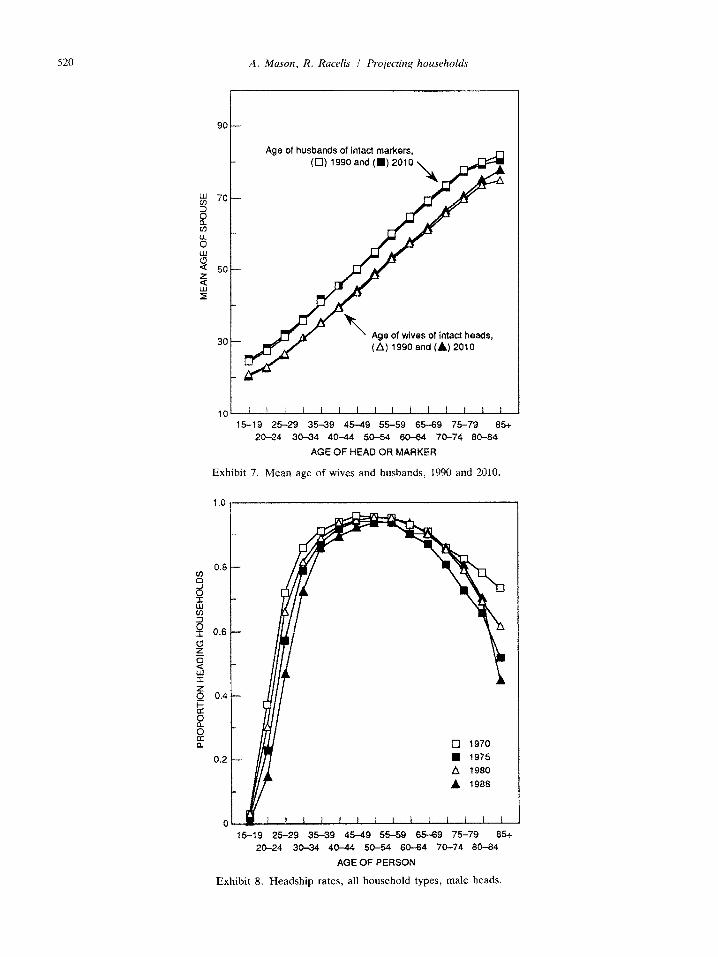
The HOMES II method produces the most significant changes in the joint age distributions of heads and spouses. For each five-year age group of heads, the mean age of wives was calculated for 1990 and 2010 and the results are plotted in Exhibit 7. Likewise, for each five-year age groups of markers, the mean age of husbands was calculated for 1990 and 2010 and also plotted in Exhibit 7. The changes projected over the 20-year period are quite modest. Young wives shift toward slightly older husbands; older wives shift toward slightly younger husbands; and, older husbands shift toward slightly older wives. Except among older heads and markers the shift in the average age of spouse is less than one year. The average age of husbands of markers 85 and older drops by 1.5 years. And the average age of wives of heads 75-79, 80-84, and 85 and older increases by 1.0, 1.2, and 2.8 years, respectively.

The other three methods entail even smaller changes in the joint age distributions of husbands

3.2. Empirical evaluation of the four methods

We offer a final comparison of the four projection methods by using the headship rates based on the 1988 National Demographic Survey to ‘backcast’ the number of households and com- pare the results with tabulations of the 1975 National Demographic Survey and samples from the 1970 and 1980 censuses. This exercise is undertaken with some trepidation because headship rates have been changing in the Philippines for reasons that are clearly unrelated to the age and sex distributions of the population (Exhibit 8). One easily could be misled to favor a particular method because of a spurious relationship between projected and observed changes in headship rates.

The empirical analysis is undertaken by projecting the number of households (heads and markers) in 1970, 1975, and 1980 using each of the four methods. The proportion of males and females heading each household type and for all household types combined is calculated using five-year age categories, 15-19 to 85+, and for all age groups combined.

The results are summarized using several measures. First, the error, efl, in the headship rates for all adults combined in year t is calculated separately for each household type i:

4, = h:, - k, . (15)

A comparison of the errors among the four methods addresses the question of which method provides a more accurate projection of the total number of households of each type.

Second, for each household type the root mean squared error (RMSE) is calculated as

RMSE = [ 0$ (h: - i;:,‘]“’ , Y

where a is the age of the head or marker (in


Intact Males. HOMES

0 2000

A 2010

03

15-19 25-29 35-39 4549 55-59 65-69 75-79 a5+ 20-24 30-34 40-44 50-54 6044 70-74 60-84

AGE OF HEAD

Intact Males. Harmonic

0 1990

. 2000

A 2010

5-19 25-29 3539 45-49 55-59 65-69 75-79 a5+

20-24 30-34 40-44 50-54 6044 70-74 60-84

AGE OF HEAD

Intact Females, HOMES

0 1990

15-19 25-29 35-39 4549 55-59 6569 75-79 a5+

20-24 30-34 40-44 50-54 60-64 70-74 60-64

AGE OF HEAD

Intact Females. Harmonic

0 1990

Ii I I I I I I I I I I I I

15-19 25-29 35-39 4549 55-59 6569 75-79 a5+

20-24 30-34 4044 5&54 60-64 70-74 60-64

AGE OF HEAD

Exhibit 6. Projected headship rates.

five-year age groups), k, is the lower age category and k, the upper age category of the age schedule of headship. Comparison of the RMSE across methods provides an assessment of reliability with which the age structure of households has been projected.

Three different RMSEs are calculated varying the upper and lower age limits. The first uses the 18 age categories that have been projected, 15- 19 to 85+. The problem with this measure is that it places undue weight on older households of which there are relatively few in the Philippines.


Intact Males, McFarland

q 1990

. 2000

A 2010

0 dl”“““““’ 15-19 25-29 35-39 4549 55-59 65-69 7579 65+

20-24 30-34 40-44 50-54 60-64 70-74 60-84

AGE OF HEAD

Intact Males, HOMES U

15-19 25-29 35-39 45-49 55-59 65-69 75-79 65+ 15-19 25-29 3539 45-49 55-59 65-69 75-79 65+

20-24 30-34 40-44 50-54 60-64 70-74 60-64 20-24 30-34 40-44 M-54 60-64 70-74 60-64

AGE OF HEAD AGE OF HEAD

Exhibit 6. Contd.

Of course, the choice of the upper age category is arbitrary in any case. The second RMSE addresses this issue by excluding headship rates for households with a head 70 and older.16

” There are better ways to do this but, as will be seen, the results are relatively insensitive to our treatment of the

upper age categories.

I-

I-

,-

OL

Intact Females, McFarland

1 I I II I I I I I 11 II 1

15-19 25-29 35-39 4!%49 55-59 65-69 7579 65+

1.0

0.2

0

X-24 3034 40-44 50-54 60-64 70-74 60-64

AGE OF HEAD

Intact Females, HOMES II

The third RMSE attempts to isolate a measure of reliability that is relatively independent of the trends in headship cited above (Exhibit 8). The major changes in the Philippines are confined to younger and older households. Headship among the middle-aged is relatively stable and apparently insensitive to the social and economic

4 I, I I I I I I I I III

520 A. Mason, R. Race& / Projecting households

90 -

$ 70-

s %

8 w

s: 50- s ii

30 -

Age of husbands of intact markers, (0) 1990 and (m) 2010

Age of wives of intact heads, (A) 1990 and (A) 2010

101 ’ ’ ’ ’ ’ ’ ’ ’ I ’ ’ ’ ’ I i 15-19 25-29 35-39 45-49 55-59 65-69 75-79 85+

20-24 30-34 4044 50-54 W-64 70-74 8584

AGE OF HEAD OR MARKER

Exhibit 7. Mean age of wives and husbands, 1990 and 2010.

0.2 -

0 1970

n 1975

o::r” 15-19 25-29 35-39 4549 55-59 65-69 75-79 85~

20-24 30-34 40-44 50-54 60-64 70-74 80-84

AGE OF PERSON

Exhibit 8. Headship rates, all household types, male heads.


Exhibit 9 Summary of projection error, intact households.

Error Males, 1970 Females, 1970 Males, 1975 Females, 1975 Males, 1980 Females, 1980

Harmonic HOMES II McFarland HOMES

0.07046 0.06947 0.10097 0.06623 0.07035 0.06938 0.10056 0.07120 0.01660 0.01579 0.03854 0.01281 0.01682 0.01599 0.03926 0.01848 0.04216 0.04149 0.05656 0.03785 0.03545 0.03475 0.05025 0.03718

RMSE” Males, 1970 0.09563 0.09530 0.15109 0.09919 Females, 1970 0.11660 0.10924 0.15324 0.11732 Males, 1975 0.03711 0.04051 0.07626 0.04236 Females, 1975 0.05526 0.03610 0.07022 0.05399 Males, 1980 0.07597 0.07334 0.09498 0.08109 Females, 1980 0.07494 0.06576 0.08321 0.07488

RMSE”

Males, 1970 0.02788 0.02338 0.06002 0.03096 Females, 1970 0.05424 0.02937 0.04068 0.04978 Males. 1975 0.01763 0.00999 0.04133 0.02134 Females, 1975 0.05248 0.01277 0.03053 0.04440 Males. 1980 0.02543 0.01870 0.04677 0.02808 Females. 1980 0.04281 0.01415 0.02901 0.03534

‘I Calculated for age categories 15-19 to 65-69. ’ Calculated for age categories 35-39 to 55-59.

changes occurring in the Philippines. The accura- HOMES II method is marginally better than the

cy with which headship rates among the middle- harmonic method. HOMES does a better job of aged are projected may provide the best guid- projecting headship rates for men but is inferior ance about the success with which the four meth- at projecting headship rates for women. The ods are tracking the impact of changes in the results are consistent with the finding presented

relative numbers of men and women. The third above that the projected number of households RMSE is confined to headship among males and is relatively insensitive to the choice among the females aged 35-59.” three methods.

The results of these analyses are presented in two summary tables. The first presents results for intact households for which changes in the availability of husbands and wives are most directly relevant. The second table presents results for all households combined. Results for all household types are reported in the Appendix, Exhibits 11-13.

The McFarland method clearly does not adapt well to the household projection problem. The overall projection error and the RMSEs are consistently higher than for the other methods in each year examined (Exhibit 9).

The overall errors for the harmonic and two HOMES methods are quite similar. The

I’ Additional calculations for the age group 35-69 have been performed but are not reported. They are quite similar to the results for the 35-59 age group.

Comparison of the RMSEs among the harmonic and HOMES methods indicates that the HOMES II method is generally more successful at projecting the age structure of households. The RMSE for households with a head 15-69 is lowest for the HOMES II method in all cases but one-the harmonic mean method produces a lower value for males in 1975. In some cases the differences are relatively minor, but for females in 1975, the HOMES II RMSE is 30% lower than for the other two methods.

The superiority of the HOMES II method is most apparent for the RMSE for middle-aged households. The values for the other methods are consistently and substantially higher, often two or three times.

Assessment of the projection errors for all households leads to conclusions that are broadly


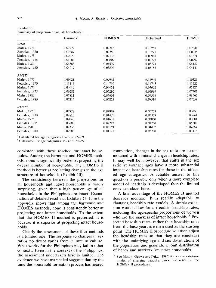
Exhibit 10 Summary of projection error, all households.

Error

Males, 1970 Females, 1970 Males, 1975 Females, 1975 Males, 1980 Females, 1980

RMSE”

Males, 1970 Females, 1970 Males. 197.5 Females, 1975 Males, 1980 Females, 1980

RMSEh

Males, 1970 Females, 1970 Males, 1975 Females, 1975 Males, 1980 Females, 1980


0.07772 0.07745 0.10258 0.07340 0.07887 0.07750 0.10225 0.08035 0.02073 0.02132 0.03908 0.01874 0.01000 0.00809 0.02723 0.00992 0.04563 0.04539 0.05774 0.04157 0.04017 0.03892 0.05185 0.04141

0.09921 0.09945 0.14949 0.10325 0.11116 0.10719 0.14745 0.11522 0.04010 0.04454 0.07602 0.05125 0.06183 0.05280 0.06969 0.07303 0.07811 0.07664 0.09598 0.08565 0.07317 0.06855 0.08510 0.07659

0.02928 0.02818 0.05763 0.03259 0.02815 0.01457 0.03369 0.03964 0.02040 0.01601 0.03860 0.03081 0.03889 0.02217 0.01760 0.05689 0.02336 0.02159 0.04407 0.02854 0.02283 0.01171 0.03200 0.03118

’ Calculated for age categories 15-19 to 65-69. h Calculated for age categories 35-39 to 55-59.

consistent with those reached for intact households. Among the harmonic and HOMES methods, none is significantly better at projecting the overall number of households. The HOMES II method is better at projecting changes in the age structure of households (Exhibit 10).

The consistency between the projections for all households and intact households is hardly surprising, given that a high percentage of all households in the Philippines are intact. Exami- nation of detailed results in Exhibits 11-13 in the appendix shows that among the harmonic and

HOMES methods, none is consistently better at projecting non-intact households. To the extent that the HOMES II method is preferred, it is because it is superior at projecting intact households.

Clearly the assessment of these four methods is a limited one. The response to changes in sex ratios no doubt varies from culture to culture. What works for the Philippines may fail in other contexts. Even in the context of the Philippines, the assessment undertaken here is limited. The evidence we have marshaled suggests that by the time the household formation process has neared

completion, changes in the sex ratio are accommodated with minimal changes in headship rates. It may well be, however, that shifts in the sex ratio at younger ages have a more substantial impact on headship rates for those in the affected age categories. A reliable answer to this question is possible only when a more complete model of headship is developed than the limited ones examined here.

A final advantage of the HOMES II method deserves mention. It is readily adaptable to

changing headship rate models. A simple extension would allow for a trend in headship rates, including the age-specific proportions of women who are the markers of intact households.” Pro- jected headship rates, rather than headship rates from the base year, are then used as the starting point. The HOMES II procedure will then adjust the headship rates so that they are consistent with the underlying age and sex distributions of the population and generate a joint distribution of heads and markers for intact households.

‘* See Mason, Ogawa and Fukui (1992) for a more extensive model of changing headship rates that relies on the HOMES II procedures.


4. Concluding remarks

Of the four methods evaluated here, the HOMES II method has a decided edge. On a priori grounds the McFarland and HOMES II method are preferable, but the McFarland method produces a very dramatic increase in headship rates for both men and women that is inconsis- tent with trends in the Philippines, or other countries for that matter. The HOMES and harmonic methods project fairly substantial changes in headship at particular ages because they do not allow for substitution across age categories. But the HOMES II method shows that the

changes in sex ratios occurring in the Philippines can be accommodated with only modest adjustments in the joint age distribution of heads and markers.

An empirical evaluation of the methods sup- ports this qualitative assessment. Households are projected backwards using the four methods and the results are compared with census and survey tabulations for 1970, 1975, and 1980. There are no important differences among the harmonic mean and HOMES methods in their accuracy in projecting the overall number of households. The HOMES II method does more accurately project the age structure of households.

Appendix

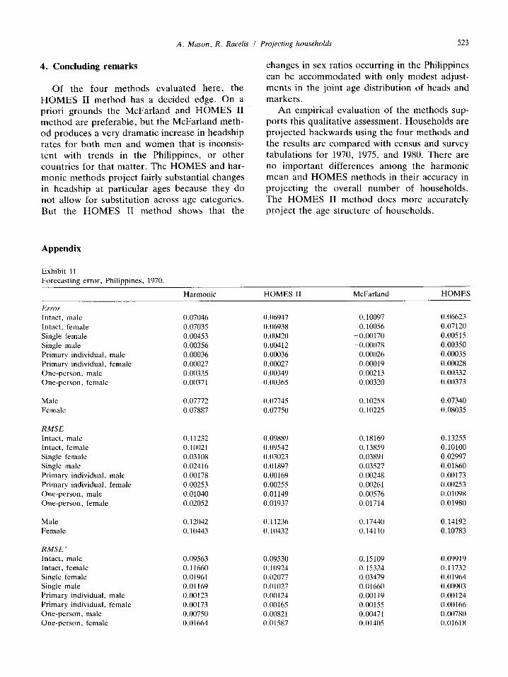
Exhibit 11 Forecasting error, Philippines, 1970.


Error Intact, male Intact, female Single female Single male Primary individual, male Primary individual, female One-person, male One-person, female

0.07046 0.06947 0.10097 0.06623 0.07035 0.06938 0.10056 0.07120 0.00453 0.00420 _ 0.00170 0.00515 0.00356 0.00412 _ -0.00078 0.00350 0.00036 0.00036 0.00026 0.00035 0.00027 0.00027 0.00019 0.00028 0.00335 0.00349 0.00213 0.00332 0.00371 0.00365 0.00320 0.00373

Male 0.07772 0.07745 0.10258 0.07340 Female 0.07887 0.07750 0.10225 0.08035

RMSE Intact, male Intact, female Single female Single male Primary individual, male Primary individual, female One-person, male One-person, female

0.11232 0.09889 0.18169 0.13255 0.10021 0.09542 0.13859 0.10100 0.03108 0.03023 0.03891 0.02997 0.02416 0.01897 0.03527 0.01860 0.00178 0.00169 0.00248 0.00173 0.00253 0.00255 0.00261 0.00253 0.01040 0.01149 0.00576 0.01098 0.02052 0.01937 0.01714 0.01980

Male 0.12042 0.11236 0.17440 0.14192 Female 0.10443 0.10432 0.14110 0.10783

RMSE” Intact, male Intact. female Single female Single male Primary individual, male Primary individual, female One-person, male One-person. female

0.09563 0.09530 0.15109 0.09919 0.11660 0.10924 0.15324 0.11732 0.01961 0.02077 0.03479 0.01964 0.01169 0.01027 0.01660 0.00903 0.00123 0.00124 0.00119 0.00124 0.00173 0.00165 0.00155 0.00166 0.00750 0.00821 0.00471 0.00780 0.01664 0.01587 0.01405 0.01618

524

Exhibit 11 (contd.)

A. Mason, R. Racelis I Projecting households

Male

Female


0.09921 0.09945 0.14949 0.10325 0.11116 0.10719 0.14745 0.11522

RMSEh

Intact, male

Intact, female

Single female

Single male

Primary individual, male

Primary individual, female

One-person, male

One-person, female

0.02788 0.02338 0.06002 0.03096 0.05424 0.02937 0.04068 0.04978 0.02277 0.01680 0.02456 0.01815 0.01424 0.01311 0.01113 0.01152 0.00118 0.00121 0.00114 0.00120 0.00179 0.00168 0.00163 0.00169 0.00876 0.00907 0.00551 0.00869 0.01525 0.01494 0.01430 0.01505

Male 0.02928 0.02818 0.05763 0.03259 Female 0.02815 0.01457 0.03369 0.03964

* Calculated for age categories 15-19 to 65-69.

h Calculated for age categories 35-39 to 55-59.

Exhibit 12

Forecasting error, Philippines, 1975.


Error Intact, male

Intact, female

Single female

Single male



One-person, male

One-person, female

Male 0.02073 0.02132 0.03908 0.01874

Female 0.01000 0.00809 0.02723 0.00992

RMSE Intact, male

Intact, female

Single female

Single male



One-person, male

One-person, female

Male 0.05282 0.04996 0.08107 0.08871

Female 0.07743 0.06893 0.07007 0.08782

RMSE” Intact, male

Intact, female

Single female Single male


Primary individual, female One-person, male

One-person, female

0.01660 0.01579 0.03854 0.01281

0.01682 0.01599 0.03926 0.01848

-0.00607 -0.00712 -0.01086 -0.00773

0.00324 0.00436 0.00050 0.00466

0.00056 0.00057 0.00050 0.00058

-0.00017 ~0.00017 -0.00023 -0.00018

0.00032 0.00060 ~ 0.00046 0.00069

-0.00058 -0.00061 -0.00094 -0.00065

0.06216 0.05177 0.09280 0.09455

0.05545 0.03677 0.06183 0.05509

0.03762 0.03975 0.05208 0.04146

0.02111 0.01552 0.02701 0.01648

0.00187 0.00191 0.00246 0.00189

0.00223 0.00214 0.00210 0.00214

0.00602 0.00571 0.00807 0.00589

0.01209 0.01273 0.01468 0.01280

0.03711 0.04051 0.07626 0.04236

0.05526 0.03610 0.07022 0.05399

0.03186 0.03474 0.04537 0.03692

0.01251 0.01131 0.01397 0.01287

0.00149 0.00151 0.00145 0.00153

0.00108 0.00101 0.00102 0.00101

0.00235 0.00256 0.00551 0.00278

0.00379 0.00370 0.00454 0.00379


Exhibit 12 (contd.)


Male 0.04010 0.04454 0.07602 0.05125 Female 0.06183 0.05280 0.06969 0.07303

RMSEh

Intact, male

Intact, female

Single female

Single male

Primary individual, male Primary individual, female

One-person, male

One-person, female

0.01763 0.00999 0.04133 0.02134

0.05248 0.01277 0.03053 0.04440

0.02160 0.02520 0.03657 0.02801

0.01503 0.01438 0.01389 0.01590

0.00090 0.00092 0.00090 0.00093

0.00098 0.00088 0.00097 0.00089

0.00186 0.00263 0.00252 0.00298

0.00477 0.00410 0.00399 0.00404

Male 0.02040 0.01601 0.03860 0.03081 Female 0.03889 0.02217 0.01760 0.05689

’ Calculated for age categories 15-19 to 65-69.


Exhibit 13

Forecasting error, Philippines, 1980.


Error

Intact, male

Intact, female

Single female

Single male



One-person, male

One-person, female

Male 0.04563 0.04539 0.05774 0.04157 Female 0.04017 0.03892 0.05185 0.04141

RMSE

Intact, male Intact. female

Single female

Single male



One-person, male

One-person, female

Male 0.07967 0.07879 0.10600 0.08286 Female 0.06848 0.06386 0.07892 0.07216

RMSE”

Intact, male

Intact, female

Single female Single male



One-person, male One-person, female

0.04216 0.04149 0.05656 0.03785

0.03545 0.03475 0.05025 0.03718

0.00145 0.00092 -0.00142 0.00096

0.00110 0.00140 -0.00072 0.00124

0.00024 0.00025 0.00022 0.00025

0.00033 0.00034 0.00030 0.00034 0.00214 0.00225 0.00168 0.00222 0.00294 0.00292 0.00273 0.00293

0.07221 0.07095 0.10374 0.07449 0.06571 0.05684 0.07248 0.06624 0.02601 0.02483 0.02759 0.02456 0.01797 0.01756 0.02359 0.01756 0.00156 0.00154 0.00177 0.00154 0.00245 0.00249 0.00257 0.00248 0.00919 0.00961 0.00602 0.00963 0.01531 0.01493 0.01377 0.01504

0.07597 0.07334 0.09498 0.08109 0.07494 0.06576 0.08321 0.07488 0.02082 0.01676 0.01933 0.01641 0.00691 0.00456 0.00796 0.00449 0.00100 0.00096 0.00096 0.00096 0.00100 0.00098 0.00094 0.00099 0.00454 0.00510 0.00325 0.00509 0.01116 0.01105 0.01069 0.01109

526

Exhibit 13 (contd.)

A. Mason, R. Racelis I Projecting households

Harmonic

Male 0.07811

Female 0.07317

RMSEh

Intact, male 0.02543

Intact, female 0.04281

Single female 0.01852

Single male 0.00806

Primary individual, male 0.00127

Primary individual, female 0.00095

One-person, male 0.00556

One-person, female 0.01230

Male 0.02336

Female 0.02283

” Calculated for age categories 15-19 to 65-69.


HOMES II McFarland HOMES

0.07664 0.09598 0.08565

0.06855 0.08510 0.07659

0.01870 0.04677 0.02808

0.01415 0.02901 0.03534

0.01077 0.01175 0.01068

0.00501 0.00835 0.00492

0.00119 0.00119 0.001 I8

0.00089 0.00085 0.00089

0.00539 0.00361 0.00536

0.01194 0.01170 0.01195

0.02159 0.04407 0.02854

0.01171 0.03200 0.03118

Acknowledgments

We wish to express our appreciation to the National Statistics Office of the Philippines and the University of the Philippines Population In- stitute for their support. Among the people who contributed to this effort, we particularly wish to acknowledge Griffith Feeney, Luisa Engracia, Corazon Raymundo, Emily Cabegin, Allen Ybaiiez, and Noreen Tanouye.

References

Akkerman. A.. 1980, “On the relationship between house-

hold composition and population age distribution”, Popu- lation Studies, 34. No. 3, 525-534.

Akkerman. A.. 1985, “The household-composition matrix as

a notion in multiregional forecasting of population and

households”, Environment and Planning, A 17, No. 3, 355-371.

Bergstrom. T. and D. Lam, 1989, “The two-sex problem and

marriage squeeze in an equilibrium model of marriage

markets”. paper presented to the Annual Meetings of the

Population Association of America, Baltimore.

Bongaarts, J., 1987, “The projection of family composition over the life course with family status life tables”, in: J.

Bongaarts, T.K. Burch and K.W. Wachter, eds., Family Demography: Methods and Their Application (Clarendon Press, Oxford). 189-212.

Brass. W.. 1083, “The formal demography of the family: An overview of the proximate determinants”, in: The Family: Proceedings of the BSPS Conference, Office of Population

Censuses and Surveys, Occasional Papers, No. 31 (OPCS, London).

Campbell, B.O. and A. Mason, 1989, “Using HOMES for

population and development planning”, United Nations

International Seminar on Population and Development

Planning, Riga, Latvian Soviet Socialist Republic. Keilman, N., 1985. “Nuptiality models and the two-sex

problem in national population forecasts”, European Journal of Population, 1, 207-235.

Keilman, N., 1988, “Dynamic household models”, in: N.

Keilman, A. Kuijsten and A. Vossen. eds., Modelling Household Formation and Dissolution (Clarendon Press,

Oxford), 123-138.

Keilman, N. and J. van Dam, 1987, “A dynamic household

projection model; An application of multidimensional

demography to lifestyles in the Netherlands”, Working Papers of the NIDI No. 72 (The Hague).

Keyfitz, N., lY71, “The mathematics of sex and marriage”,

in: Proceedings of the Sixth Berkeley Symposium on Mathematical Statistics and Probability (University of

California Press, Berkeley), 89-108.

Kono, S., 1987, “The headship rate method for projecting

households”, in: J. Bongaarts. T.K. Burch and K.W.

Wachter, eds.. Family Demography: Methods and their Application (Clarendon Press. Oxford), 287-308.

Linke, W., 1988, “The headship rate approach in modelling

households: The case of the Federal Republic of Ger-

many”, in: N. Keilman, A. Kuijsten and A. Vossen, cds.,

Modelling Household Formation and Dissolution (Claren-

don Press, Oxford), 1088122. Mason. A., 1987, HOMES: A Household Model for

Economic and Social Studies, Papers of the East-West

Population Institute, No. 106, Honolulu. Mason, A., N. Ogawa and T. Fukui, 1992, Household Pro-

jections for Japan, 1985-202S: A Transition Model of Headship Rates (Japan Statistical Association, Nihon Uni-

versity Population Research Institute, Tokyo. and the

East-West Center). McFarland, D., 1975, “Models of marriage formation and

fertility”, Social Forces. 54. No. 1, 66-83.

A. Mason. R. Racelis I Projecting household.~ 527

Murphy, M.. 1YYla. “Household modelling and forecasting: Dynamic approaches with use of linked census data”,

Environmenr und Plunning, A 23. 885-002.

Murphy. M., IYY 1 b, “Modelling households: A synthesis”, in

M. Murphy and J. Ho&raft. eds., Population Research in

Brituin. Supplement to Populution Studies. 45, 157-176. Pitkin, J.R. and G.S. Masnick, 1987, “The relationship

between heads and non-heads in the household popula-

tion: An extension of the headship rate method”, in: J.

Bongaarts. T.K. Burch and K.W. Wachter. eds. Fumi/y

Demography: Methods und Their Applicution (Clarendon

Pres\. Oxford). 309%326.

Pollak, R.A.. lY86. “A reformulation of the two-sex prob-

lem”, Demography, 23. No. 2. 247-259.

Pollak, R.A.. IYYO. “Two-sex demographic models”. Journul

of Political Economy, Y8, No. 2. 3YYS420.

Pollard. J.H., 1973. Mathematical Models for the Growth of

Humun Populations (Cambridge University Press, Cam-

bridge).

Pollard, J.H., 1977, “The continuing attempt to incorporate

both sexes into marriage analysis”, Inrernationul Popula-

tion Conference: Mexico lY77 (IUSSP, Liege). 29 l-310.

Preston. S.H., IYXY, “Marriage and divorce data in theoreti-

cal population studies”. Challenges for Public Health

Stutistics in the I YYOs, Proceedings of the I WY Public

Health Conference on Records and Stutisrics, l7- IY July,

Washington, D.C. Ruggles. S.. 1087. Prolonged Connections: The Rise of the

Extended Fumily (University of Wisconsin Press,

Madison).

Schoen, R.. 1081. “The harmonic mean as the basis of a

realistic two-sex marriage model”, Demogruphy. IX, No.

2, 201~216.

United Nations. lY73, Murw11 VII. Methods of Projectmg

Households und b’umilies (United Nations, New York).

US Bureau of Census. lY7Y. Current Populution Reports,

Series P-25. No. 805 (May).

Biographies: Andrew MASON is Director of the Program on Population. East-West Center and Professor of Economics. University of Hawaii.

Rachel RACELIS was a Research Associate, Program on Population, East-West Center at the time that this paper was prepared. She is currently working as a consultant in the Philippines

A comparison of four methods for projecting households

Documents

Transcript of A comparison of four methods for projecting households