1

A Comparison of Four Factor Analytical Methods Used with Ordinal Data

Margaret Sanders

The Royal Shakespeare Company created the Stand Up for Shakespeare (SUFS) program

to change the way students encounter Shakespeare in school. The program prepares teachers to

help students engage with Shakespeare the way actors would—interacting with the plays as

scripts to be acted rather than texts to be read. Through this pedagogy, SUFS aims to increase

students’ interest in Shakespeare and both their interest and ability in reading. The most thorough

evaluation of the SUFS program (Strand, 2009) used factor analysis to examine the structure of

attitudes toward Shakespeare and found it to be unidimensional and reliable (Cronbach’s α =

0.85). The resulting factor scores correlated somewhat with academic self concept (r = 0.22) and

school engagement (r = 0.37), but not with attainment in Language Arts. However, despite

measuring student attitudes on an ordinal scale, many of the analyses utilized methods that

assume continuous and normally distributed data, consistent with findings that ordinal data are

often treated inappropriately in analyses in applied research (Kampen & Swyngedouw, 2000).

Because ordinal data are the norm in education research but are also frequently analyzed

incorrectly, this study explored the internal structure of the SUFS data, including the stability of

the factor structure, to illustrate how more and less appropriate analytic decisions manifest in real

data characteristic of the field. More importantly, it compared four factor analytic methods head-

to-head to determine which produced the most stable factor structure, validated by a CFA on data

gathered at two time points. The four methods included a traditional exploratory factor analysis

(EFA), a full-information or ordinal EFA (Jöreskog & Moustaki, 2006), and two exploratory

factor analyses within the confirmatory factor analysis framework (E/CFA); one according to the

Jöreskog model specification search method (1969; Jöreskog & Sörbom, 1979), and the other

2

according to the Gugiu method (Gugiu, 2011; Gugiu, Coryn, Clark, & Kuehn, 2009). These

methods differed in the observed input correlation matrix, the method of estimation used to

extract factors, the method of factor selection, and the method of model modification used in

refining the models. The appropriateness and strength of the four methods were assessed by

determining how well the extracted models replicated in an independent data set.

Traditional EFA

Before discussing the traditional EFA method, it is worth drawing a distinction between

factor analysis and principal components analysis (PCA). The two methods are similar and often

confused, but only factor analysis is appropriate for exploring latent factor structure such as the

SUFS survey of attitudes toward Shakespeare. The difference lies in how the two methods model

variance. PCA models variance with components, which are a linear combination of all of the

variance in the set of indicators used in the PCA. Factor analysis, on the other hand, models

variance using latent factors, a linear combination of only the common variance in the set of

indicators used in the EFA (Tabachnick & Fidell, 2001). Thus, the first step is to determine

whether one is interested in modeling all of the variance (PCA) or just the common variance

(EFA). In general, if a common trait or construct is thought to predict a set of behaviors,

indicators, or responses to a set of items, then the appropriate method is EFA, not PCA.

The second step is to define the input correlation matrix that will be modeled with latent

factors in the EFA. Input matrixes are most commonly generated using the Pearson product-

moment correlation coefficient, which assumes that the data are continuous and bivariate normal.

However, using the Pearson coefficient to calculate correlations for ordinal variables decreases

variability, as all scores within a given range on the latent factor are assigned to the same

category of the observed variable. This reduced variability leads to underestimated associations

3

between variables (Gilley & Uhlig, 1993), as well as decreased parameter estimates in factor

analyses using Pearson correlation matrixes as input (DiStefano, 2002; Olsson, 1979). To

illustrate the impact of inappropriately inputting a Pearson correlation matrix with non-normal

and non-continuous data, the matrix was used in the traditional EFA with the SUFS data.

Factor selection—arguably the most important step of factor analysis—uses the

correlation matrix produced in factor extraction to calculate the number of factors that should be

retained in subsequent analyses. Scree plots and the Kaiser criterion are frequently used to select

factors although the accuracy of these methods is questionable (Hayton, Allen, & Scarpello,

2004). Owing to its popularity among researchers, a scree plot was used in the traditional EFA.

After the input correlation matrix is specified, the next step is to select a method for estimating

the factor model. The most frequently used method of estimation is maximum likelihood (ML),

which is appropriate for use when data are continuous and normal (Brown, 2006). Thus, ML was

used in the traditional EFA, despite being inappropriate given the ordinal nature of the data.

Once estimated, the original model may be modified by eliminating items with factor

loadings that fall below a threshold of 0.3 (Tabachnick & Fidell, 2001). Below this threshold, the

latent factors account for less than 10% of the variance in the item. Therefore, these items are not

strong indicators of the latent variable and can be eliminated. Finally, reliability of the final

model is typically, though problematically, estimated by Cronbach’s alpha. Similar to other

standard procedures, Cronbach’s alpha misestimates reliability unless specific conditions hold,

such as tau equivalence and the absence of correlated measurement errors (Brown, 2006).

Full-information EFA

The full-information or ordinal EFA (Jöreskog & Moustaki, 2006) differs from the

traditional EFA in the coefficient used for the input correlation matrix, the method of factor

4

selection, and the reported reliability statistic. First, ordinal EFA uses the polychoric correlation

coefficient rather than the Pearson correlation coefficient. This coefficient is estimated from the

bivariate frequency distribution (crosstab) of the observed ordinal scores, under the assumption

of bivariate normality. The estimated relationships are closer to the correlations found if the

variables were measured on an interval rather than ordinal scale (Brown, 2006), Consequently,

the coefficients are more accurate, yielding less attenuated parameter estimates in factor analysis.

Factors were selected using parallel analysis rather than a scree plot. This method plots

the eigenvalues calculated from the actual data (akin to a scree plot) against the eigenvalues

generated from random data that matches key characteristics of the actual data, including the

sample size and number of variables. The eigenvalues are plotted in descending magnitude, and

the point at which the two plotted lines cross indicates the number of factors to retain. Thus, a

factor is worth retaining when its associated eigenvalue is greater than the eigenvalue expected

by chance alone. After factor selection and model estimation, items with loadings less than 0.3

are eliminated, paralleling the modification process in the traditional EFA method. The reliability

of the full-information EFA model is reported in terms of Raykov’s (2001, 2004) coefficient of

scale reliability ρ, which avoids many of the problems associated with Cronbach’s alpha.

E/CFA

Similar to the full-information EFA, the Jöreskog and Gugiu E/CFA methods utilize the

polychoric correlation matrix as input, parallel analysis to select factors, and Raykov’s (2001,

2004) coefficient ρ to measure reliability. However, both E/CFA methods have a distinct

advantage over the traditional and the full-information EFAs in using CFA to estimate the EFA

models, thereby producing fit statistics that can be used to refine the initial model. This

specification search tends to produce better fitting initial models that are more likely to replicate

5

in an independent CFA (Brown, 2006). Furthermore, both E/CFA methods use a different factor

extraction method; namely, diagonal weighted least squares (DWLS) in conjunction with the

asymptotic covariance matrix. Unlike ML, DWLS and the asymptotic covariance matrix adjust

parameter estimates for violations of normality and so are appropriate for use with non-normal

and categorical data (Brown, 2006). The asymptotic covariance matrix is used to compute a

weight matrix used to adjust the fit statistics and standard errors for nonnormality (Brown, 2006).

Essentially, items with less asymptotic variance (i.e., greater precision) are given more weight

than variables with more variance (i.e., more sampling error) (Schumacher & Lomax, 2010).

Although similar in specification search and extraction method, the two methods of

E/CFA differ in model modification. The Jöreskog approach (1969; Jöreskog & Sörbom, 1979)

relies on identifying large modification indices (MI) in an initial model. MIs represent the

amount the model chi-square will decrease if the corresponding correlated error is freed. Freeing

errors with MIs greater than 3.84, the critical chi-square value at α = 0.05, will result in

significantly better model fit, as indicated by a significant χ2 difference test between the simpler

(nested) and more complex (null) model. Because freeing a single significant MI can have

substantial and unpredictable effects on model fit indices, significant MIs should be freed one at

a time in a recursive process. Furthermore, the correlated errors corresponding to the MI should

only be freed if substantially justified by theory. After the highest correlated error is freed, the

modified model is compared to the previous model using a χ2 difference test, and this process is

repeated until both the χ2 for the model and the χ2 difference test are nonsignificant, indicating

that the last freed error covariance did not significantly improve model fit.

An alternative method of model specification within the E/CFA framework is the Gugiu

approach (Gugiu, 2011; Gugiu et al., 2009). Rather than freeing correlated errors, this approach

6

deletes items from the model that contribute to model misfit. Candidates for deletion are selected

by examining the residual table for the largest misfitting standardized residual. When greater

than 1.96 in absolute value (critical value at α = 0.05), standardized residuals represent the

difference between the estimated and observed covariances divided by the asymptotic standard

errors—the square root of the asymptotic variance. Thus, the two items that correspond to this

covariance contribute a great deal to the model misfit. To reduce model misfit, the item with the

greatest number of misfitting standardized residuals is removed from the model. Similar to the

Jöreskog method, each reduced model is compared to the previous models, and the process is

repeated until the χ2 difference test is nonsignificant. Although the Jöreskog method relies

primarily on MIs whereas the Gugiu method relies on standardized residuals, both approaches

use additional information provide by the CFA framework to refine the initial models.

Model Comparison

In the current study, models of the SUFS pretest data were specified according to the four

methods of factor analysis and then a confirmatory factor analysis (CFAs) was performed on the

posttest data. SAS 9.3 was used to specify the traditional EFA model and the full-information

EFA model; all other model specification and validation was conducted in LISREL 8.8. The

EFAs specified in SAS were also run in LISREL to obtain model fit statistics, which are not

normally produced in an EFA framework.

Models were compared based on four goodness-of-fit statistics, the number of misfitting

standardized residuals and significant MIs, and reliability. The first goodness-of-fit statistic used

was the χ2 statistic for the model, which indicates whether the difference between the observed

and estimated model is significant. A nonsignificant χ2 statistic suggests that the model fits the

data well. The normal theory weighted least squares χ2 (NTWLS χ2) is appropriate when data are

7

normal, whereas the Satorra-Bentler scaled χ2 (SB χ2; Satorra & Bentler, 1994) is appropriate

when data do not meet the normality assumption. The models were also compared in terms of the

root mean square error of approximation (RMSEA), which measures absolute fit with a penalty

for non-parsimonious models (Brown, 2006). A RMSEA value of 0 indicates perfect fit, while

values less than or equal to 0.05 indicate that the model fits the data well. The standardized root

mean square residual (SRMR), a measure of absolute fit, was also used to compare the models.

SRMR values below 0.05 indicate good model fit, with smaller values indicating better fit. The

last goodness-of-fit statistic used was the Tucker-Lewis index (TLI). Like RMSEA, TLI also

includes a penalty for model complexity but measures model fit relative to the null model. The

closer the TLI value is to 1.0 the better the model; TLI values above 0.95 are desirable.

Models were also compared in terms of the number of observed and expected misfitting

standardized residuals and significant MIs. The number of misfitting residuals or significant MIs

expected by chance may be calculated by , where k denotes the number of

variables, is the total number of residuals or MIs, and p is the Type I error rate

(Gugiu et al., 2009). A larger-than-expected number of observed misfittting standardized

residuals or significant MIs suggests that the model does not capture important relationships in

the data. Models were compared in terms of whether and by how much they exceeded the

number of misfits expected by chance. Finally, the reliabilities of the models were also compared

to assess the stability of the latent scores produced by each model.

Method

Sample

Schools and teachers in a large, midwestern city were recruited to participate in the SUFS

drama-based pedagogy program: 503 students participated in the study (54% female; 5% Asian,

p∗ k(k −1) / 2

k(k −1) / 2

8

15% Black or African American, 4% Hispanic, 18% multi-racial, 49% white, 10% not reported).

These students ranged from grades 3 to 8 and were drawn from the classrooms of 14 teachers

across 5 schools in 2 public school districts.

Instrument

In September 2011 and May 2012, students were administered a survey about their

exposure to Shakespeare, attitudes toward Shakespeare, and attitude toward school. This was

modeled on the Warwick survey administered in England (Strand, 2009). Questions pertaining to

Shakespeare were measured on a 3-point scale: “No” (1), “Don’t Know” (2), and “Yes” (3).

Although it is unclear where “Don’t Know” should logically fall on the dimension of “No” to

“Yes,” a Rasch analysis revealed that students treated “Don’t Know” as a middle point

(Yeomans-Maldonado, Gugiu, & Enciso, 2013). Thus, instead of dichotomizing the scale by

collapsing the “Don’t Know” responses into the “No” category, the 3-point ordinal scale was

retained. This study focused on the 12 questions about student attitudes toward Shakespeare.

Procedure

Teachers collected permission from parents for students to participate in the study. A

survey was administered before students had been exposed to the SUFS pedagogy and again

after teachers had implemented SUFS pedagogy. Research assistants read the questions out loud

to students at the end of a regular class period, and students who did not have permission to

participate were asked to sit quietly.

Results

Missing Value Imputation

The original sample of 503 was reduced to 400 after cases with more than 30% missing

responses and students who only completed either the pretest or the posttest were removed from

9

the sample. The missing response rate per question in the final sample ranged from 0.5% to 3%.

Because list- and pair-wise deletion would have further reduced the size of the sample, thereby

potentially resulting in a sampling bias, missing values were imputed using multiple imputation.

Although missing values are often replaced with the variable mean or a single regression-

imputed value, these simple imputation methods tend to underestimate variance and overestimate

covariance (Brown, 2006). Multiple imputation, however, reintroduces random variance into

regression imputation by imputing multiple datasets with slightly different estimates, combining

the estimates across the datasets, and replacing missing values with these composites. Following

this method, five imputations (Yuan, 2000) of the SUFS data were conducted using the

expectation maximization algorithm and Markov Chain Monte Carlo method. Because the

between sample variance was incredibly low for each imputed variable—0.00005 at most—the

five imputed data sets were averaged into a single data set used for all subsequent analyses.

Nature of the Data

Before selecting a method of analysis, the normality and continuity of the data at both the

latent and indicator levels must be established because these characteristics constrain the type of

analyses that may appropriately be conducted. In the case of the SUFS data, attitudes toward

Shakespeare is probably continuous and normal at the latent level because fine-grained

differences in attitudes can be distinguished along a continuum. Furthermore, in the population,

people’s feelings about Shakespeare are likely unimodal and symmetrically distributed about a

mean. PRELIS was used to test the bivariate assumption of each correlation, with 71% of the 66

correlations in the 12-item set passing this test; in the set reduced by the item deletion of the

Gugiu method, 52% of the 21 correlations passed the bivariate normality test. At the observed

variable level, each item displayed significant skew, kurtosis, or both, suggesting that the data’s

10

distribution differed significantly from normal; the 3-point scale was categorical, falling below

the 15-point cut off normally considered continuous (Jöreskog & Sörbom, 1996; Schumacher

& Lomax, 1996). Thus, it is reasonable to conclude that the SUFS data was approximately

normal and continuous at the latent level and non-normal and categorical at the indicator level.

Factor Selection

In the traditional EFA, a scree plot was used to select factors from the Pearson correlation

matrix and indicated that one factor should be retained. In the other three factor analyses, parallel

analysis was used to select factors from the polychoric correlation matrix and indicated that one

factor should be retained, in this case consistent with the scree plot. Hence, this study could not

compare the impact of using scree plot and parallel analysis as methods of factor selection.

Model Specification Search

Traditional EFA. All 12 items in the traditional EFA loaded on the latent factor above the

0.3 threshold and so were retained in the model. The goodness of fit statistics indicated that the

final model did not fit the observed data particularly well (see Table 1). Furthermore, the

observed number of misfitting residuals (20) and significant MIs (20) in the EFA model

exceeded the number expected (3.3), suggesting considerable model misfit. The model reliability

was acceptable as measured by Cronbach’s alpha, α = 0.845 and acceptable according to

Raykov’s ρ = 0.847 (calculated so the reliability of all four models could be compared).

Full-information EFA. As was the case in the traditional EFA, all 12 items in the full-

information EFA loaded on the latent factor above the 0.3 threshold and thus were retained in the

model (see Figure 1). Although the conceptual model was the same for both the traditional and

the full-information EFAs, the goodness-of-fit indices and model reliability improved as a result

of employing the polychoric correlation matrix and DWLS estimation method. Furthermore, the

11

8 observed misfitting standardized residuals and 13 significant MIs were both closer to the

expected number of misfits (3.3) (see Table 1). Similarly, the reliability of the full-information

EFA was greater than that of the traditional EFA, ρ = 0.903. Moreover, the difference in the

parameter estimates between the traditional EFA and the full-information EFA is important to

note (see Table 2). Systematically, the full-information EFA produced greater factor loadings

than the traditional EFA, while the full-information EFA error variance estimates were smaller.

Jöreskog E/CFA. In the SUFS dataset, all items could reasonably be related to one

another, as all focused on some aspect of students’ attitude toward Shakespeare. Therefore,

correlated errors were freed beginning with the error associated with the largest MI until both the

SB χ2 for the model and the SB χ2 difference test were nonsignificant (see Table 3). Following

this approach resulted in a final modified model with 9 freed error covariances (see Figure 1).

The goodness-of-fit indices for the model built with this approach showed significant

improvement over the previous EFAs (see Table 1). Examination of the standardized residuals

and MIs also indicated very good model fit with no misfitting standardized residuals and fewer

than expected significant MIs. Furthermore, the reliability of the E/CFA model was higher, ρ =

0.951, and the parameter estimates greater than in the traditional EFA (see Table 2).

Gugiu E/CFA. Through the process of identifying large residuals, deleting corresponding

items, and computing the SB χ2 difference test, 5 items were removed, resulting in a final model

that included 7 items (see Table 4 and Figure 1). To avoid overfitting the model, a reasonable

case could have been made for retaining the last item (question 9), given the very small and

nonsignificant SB χ2 value, the well-fitted model indicated by the goodness-of-fit indices, and

the fewer-than-expected observed misfitting standardized residuals and significant MI. However,

the 7-item model was used as the final model because model fit improved and the construct

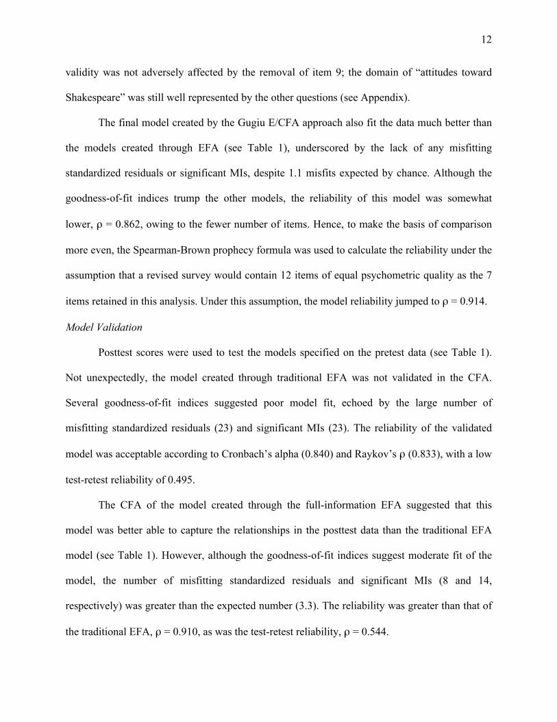
12

validity was not adversely affected by the removal of item 9; the domain of “attitudes toward

Shakespeare” was still well represented by the other questions (see Appendix).

The final model created by the Gugiu E/CFA approach also fit the data much better than

the models created through EFA (see Table 1), underscored by the lack of any misfitting

standardized residuals or significant MIs, despite 1.1 misfits expected by chance. Although the

goodness-of-fit indices trump the other models, the reliability of this model was somewhat

lower, ρ = 0.862, owing to the fewer number of items. Hence, to make the basis of comparison

more even, the Spearman-Brown prophecy formula was used to calculate the reliability under the

assumption that a revised survey would contain 12 items of equal psychometric quality as the 7

items retained in this analysis. Under this assumption, the model reliability jumped to ρ = 0.914.

Model Validation

Posttest scores were used to test the models specified on the pretest data (see Table 1).

Not unexpectedly, the model created through traditional EFA was not validated in the CFA.

Several goodness-of-fit indices suggested poor model fit, echoed by the large number of

misfitting standardized residuals (23) and significant MIs (23). The reliability of the validated

model was acceptable according to Cronbach’s alpha (0.840) and Raykov’s ρ (0.833), with a low

test-retest reliability of 0.495.

The CFA of the model created through the full-information EFA suggested that this

model was better able to capture the relationships in the posttest data than the traditional EFA

model (see Table 1). However, although the goodness-of-fit indices suggest moderate fit of the

model, the number of misfitting standardized residuals and significant MIs (8 and 14,

respectively) was greater than the expected number (3.3). The reliability was greater than that of

the traditional EFA, ρ = 0.910, as was the test-retest reliability, ρ = 0.544.

13

The models created by the two E/CFA methods both fared better in validation than the

models created through EFA. The model specified by the Jöreskog method was able to capture

the relationships in the posttest data very well, as demonstrated by the goodness-of-fit indices

(see Table 1), but examination of the standardized residuals and MIs suggested there were

associations in the posttest data that were not well represented by the model (8 significant MIs

observed and 3.3 expected). In particular, the pattern of significant MI and corresponding error

covariances to free differed between the pretest and posttest data. Of the nine freed correlated

errors in the model of the pretest data, only four were significantly different from zero in the

posttest data (see Table 5). Similarly, the posttest CFA highlighted eight large MI that were

negligible in the pretest model. Of the 132 possible MI, the pre- and posttest models differ on 13,

representing 10% disagreement. Despite these inconsistencies, the model showed a high degree

of reliability, ρ = 0.938, and an acceptable level of test-retest reliability, ρ = 0.559.

The Gugiu E/CFA model also fit the posttest data associations better than the EFAs, but

slightly less well than the Jöreskog E/CFA model (see Table 1). As with the other models, the

misfitting standardized residuals (1) and significant MIs (6) suggested some lack of fit (1.1

expected). The reliability was lower than that of the Jöreskog E/CFA model, ρ = 0.864, as was

the test-retest reliability, ρ = 0.525. However, when estimated with 12 items instead of 7 using

the Spearman-Brown prophecy formula, the internal (ρ = 0.916) and test-retest (ρ = 0.655)

reliabilities were comparable to those of the Jöreskog E/CFA model.

Discussion

Several lessons can be learned from the results of these models. First, it is clear that using

analyses whose assumptions are incompatible with the nature of the data can have severe

implications for the results. In the case of the traditional EFA, an inappropriate correlation matrix

14

resulted in underestimated factor loadings and contributed to poor model fit, as compared to the

results of the full-information EFA. Unfortunately, ordinal type—the norm in applied education

research—does not meet the assumptions of most of the methods of statistical analysis. Thus,

traditional EFAs are generally not recommended unless data are continuous.

The goodness-of-fit indices suggest that the full-information EFA estimates did a slightly

better job of capturing the observed relationships than those produced by the traditional EFA.

The impact of using a polychoric correlation matrix rather than the Pearson correlation matrix is

highlighted by the difference in the parameter estimates between the traditional EFA and full-

information EFA (see Table 2). Because the Pearson estimates relationships from the coarse

categories rather than continuous scores, it underestimates the associations between variables,

which manifests in smaller parameter estimates and poorer model fit statistics. Although the full-

information EFA is appropriate given the nature of the data and provides better model fit than the

traditional EFA, ultimately it is also not an ideal method of factor analysis. Without the ability to

refine EFA models, not only does the model exhibit relatively poor fit, but the odds of it being

validated by a CFA are also quite low, as was illustrated in this study. Thus, the EFA approach to

model specification, regardless of whether the analysis is appropriate to the nature of the data, is

of questionable use. Given the limited initial model fit and subsequent failure to validate, we do

not recommend the use of EFA for the purpose of establishing internal validity of a survey

instrument, particularly when the stability of the latent construct over time is important.

Fortunately, both E/CFA methods avoided the problems encountered by the two EFAs,

thereby yielding robust initial models that also fit the data well in a CFA context. However, the

Jöreskog method faced a challenge not faced by the other three methods; namely, what

constitutes a sufficiently substantive, theory-based rationale for freeing correlated errors. In the

15

case of this study, it is unclear how the presence of so many correlated errors can be justified,

particularly because the reason used to justify the presence of a correlated error must also explain

why it does not apply in the case of absent correlated errors. On this basis, it is not intuitive why

these nine pairs of questions share significant amounts of variance with each other but not the

other items (see Appendix), and an a priori theoretical prediction of these relationships is highly

unlikely. If only the errors that could be substantively justified were freed, as is often

recommended, then the Jöreskog model in this study would have resembled that of the full

information EFA as few, if any, of the correlated errors could be substantiated on theoretical

grounds. That being the case, the performance of the Jöreskog E/CFA method would have

resembled that of the full information EFA.

Furthermore, not only is the pattern of correlated errors difficult to justify and interpret,

but the overall model is less stable. The size and significance of 10% of the MI differed between

the pre- and posttest models, representing a small but non-ignorable amount of instability. This

may result from the use of a 3.84 (critical value at α = 0.05) cut-off for large MIs, which may not

be appropriate when used in conjunction with DWLS. The interpretation of MIs as chi-square

difference is only appropriate for ML or robust maximum likelihood (RML) estimation methods

with continuous variables; MI values are not directly analogous to chi-square differences under

DWLS (K. Jöreskog, personal communication, June 23, 2013). In other words, the significance

of MIs cannot be interpreted in the same way with the type of data found in the SUFS study.

Therefore, even though the Jöreskog E/CFA method produced well-fitting models that were

validated by a CFA on posttest data, the interpretability and instability of the models, as well as

the uncertain appropriateness of the MI criteria, suggest that this method may also not yield

stable results for applied education research.

16

The Gugiu E/CFA method is not limited by the issues of other methods but still produced

well-fitting models that replicated in posttest CFAs. To its credit, the method produces models

without correlated errors that are more easily interpretable than Jöreskog E/CFA models and that

do not require ad hoc theoretical justifications. The method places a greater emphasis on

standardized residuals than on MIs as a modification criterion and thus may be used with

categorical and non-continuous data without concerns regarding the interpretation of the

modification criteria. However, the limited number of items retained by this method does raise

two concerns. First, with fewer items, models may be less reliable, a fact reflected in the models

of the SUFS data. Second, iteratively reducing the number of items runs the risk of decreasing

the model’s construct validity. Fortunately, these issues can be easily addressed by adding more

items and retaining items that are theoretically important for the construct. As suggested by the

Spearman-Brown prophecy formula, adding more items with parallel psychometric properties

will increase the reliability of these models to levels comparable to, if not better than, the

reliability of models created through the other methods. Therefore, to the degree to which one

can generalize from a single study, it would appear that the Gugiu E/CFA method produces a

more stable and interpretable factor structure than the other three methods employed in this

study. Considerably more research is needed to further vet this method in order to fully

understand its strengths and weaknesses; however, it does offer a promising approach for factor

analyzing the type of data most frequently encountered in education research.

17

References

Brown, T. A. (2006). Confirmatory factor analysis for applied research. Guilford Press. DiStefano, C. (2002). The impact of categorization with confirmatory factor analysis. Structural

Equation Modeling, 9(3), 327-346. Gilley, W., & Uhlig, G. (1993). Factor analysis and ordinal data. Education, 114(2), 258-264. Gugiu, P. C., Coryn, C., Clark, R., & Kuehn, A. (2009). Development and evaluation of the short

version of the Patient Assessment of Chronic Illness Care instrument. Chronic Illness, 5(4), 268-276.

Gugiu, P. C. (2011, November). Exploratory Factor Analysis within a Confirmatory Factor Analysis Framework (E/CFA). Expert lecture presented at the 2011 American Evaluation Association conference in Anaheim, California.

Hayton, J. C., Allen, D. G., & Scarpello, V. (2004). Factor retention decisions in exploratory factor analysis: A tutorial on parallel analysis. Organizational Research Methods, 7(2), 191-205.

Jöreskog, K. G. (1969). A general approach to confirmatory maximum likelihood factor analysis. Psychometrika, 34(2), 183-202.

Jöreskog, K. G., & Sörbom, D. (1979). Advances in factor analysis and structural equation models (p. 105). J. Magidson (Ed.). Cambridge, MA: Abt Books.

Jöreskog, K. G., & Sörbom, D. (1996). LISREL 8: User's reference guide. Lincolnwood, IL: Scientific Software International.

Jöreskog, K. G. & Moustaki, I. (2006). Factor analysis of ordinal variables with full information maximum likelihood. Hillsdale, NJ: Lawrence Erlbaum Associates.

Kampen, J., & Swyngedouw, M. (2000). The ordinal controversy revisited. Quality and Quantity, 34(1), 87-102.

Olsson, U. (1979). On the robustness of factor analysis against crude classification of the observations. Multivariate Behavioral Research, 14(4), 485-500.

Raykov, T. (2001). Estimation of congeneric scale reliability using covariance structure analysis with nonlinear constraints. British Journal of Mathematical and Statistical Psychology, 54(2), 315-323.

Raykov, T. (2004). Behavioral scale reliability and measurement invariance evaluation using latent variable modeling. Behavior Therapy, 35(2), 299-331.

Satorra, A., & Bentler, P. M. (1994). Corrections to test statistics and standard errors in covariance structure analysis. In A. von Eye & C. Clogg (Eds.), Latent variable analysis: Applications for developmental research (pp. 399-419). Thousand Oaks, CA: Sage.

Schumacher, R. E. & Lomax, R. G. (1996). A beginner's guide to SEM. Manwah, NJ: Lawrence Erlbaum Associates.

Strand, S. (2009). Attitude to Shakespeare among Y10 students: Final report to the Royal Shakespeare Company on the Learning and Performance Network student survey 2007-2009. Warwick, England: Centre for Educational Development, Appraisal and Research.

Tabachnick, B. G., & Fidell, L. S. (2001). Using multivariate statistics. Boston: Pearson. Yeomans-Maldonado, G., Gugiu, C. P., & Enciso, P. (2013, May). Using the Rasch model to

assess the interest for Shakespeare and illustrate rating scale diagnostics. Poster presented at the Modern Modeling Methods Conference, Storrs, CT.

Yuan, Y. C. (2000). Multiple imputation for missing data: Concepts and new development (SAS Tech. Rep. No. P267-25). Rockville, MD: SAS Institute.

18

Appendix

Attitudes Toward Shakespeare Survey, Based on Warwick Survey (Strand, 2009)

What I think about Shakespeare Don’t know

1. Everyone should read Shakespeare No ! ! Yes !

2. Shakespeare is fun No ! ! Yes !

3. Shakespeare’s plays are difficult for me to understand No ! ! Yes !

4. Shakespeare’s plays help us understand each other better No ! ! Yes !

5. I would like to do more Shakespeare No ! ! Yes ! 6. Some of the people in Shakespeare’s plays are like people

you meet today No ! ! Yes !

7. I tell my friends in other classes about Shakespeare No ! ! Yes !

8. It is important to study Shakespeare’s plays No ! ! Yes !

9. Shakespeare is only for old people No ! ! Yes ! 10. Things that happen in Shakespeare’s plays can happen in

real life No ! ! Yes !

11. Shakespeare is boring No ! ! Yes ! 12. I have learned something about myself by learning about

Shakespeare No ! ! Yes !

Table 1 G

oodness-of-Fit Indices for Models of Attitude Tow

ard Shakespeare (n=400)

Model B

uilding: Pretest Sample

Final Model

χ2

df R

MSEA

(90%

CI)

SRM

R

NN

FI (TLI)

Expected M

isfits c O

bserved Misfits

(Residuals, M

I) R

aykov’s R

eliability

EFA

207.599***a

54 0.084

(0.072, 0.097) 0.056

0.948 3.3

20, 20 0.847

EFA

(polychoric) 146.675***

b 54

0.066 (0.053, 0.078)

0.063 0.978

3.3 8, 13

0.903

E/CFA

(Jöreskog)

46.516b

45 0.009

(0.000, 0.035) 0.038

1.000 3.3

0, 1 0.951

E/CFA

(G

ugiu) 4.569

b 14

0.000 (0.000, 0.000)

0.020 1.007

1.1 0, 0

0.862

Model V

alidation: Posttest Sample

Final Model

χ2

df R

MSEA

(90%

CI)

SRM

R

NN

FI (TLI)

Expected M

isfits c O

bserved Misfits

(Residuals, M

I) R

aykov’s R

eliability Test-R

etest

EFA

291.886***a

54 0.105

(0.093, 0.117) 0.065

0.914 3.3

23, 23 0.833

0.495

EFA

(polychoric) 151.127***

b 54

0.067 (0.055, 0.080)

0.069 0.979

3.3 8, 14

0.910 0.544

E/CFA

(Jöreskog)

74.014**b

45 0.040

(0.023, 0.056) 0.048

0.993 3.3

3, 8 0.938

0.559

E/CFA

(G

ugiu) 28.896*

b 14

0.052 (0.024, 0.078)

0.050 0.989

1.1 1, 6

0.864 0.525

a Norm

al Theory Weighted Least Squares χ

2. b Satorra-Bentler χ

2. c Refers to either the num

ber of expected misfitting

standardized residuals or the number of expected significant m

odification indices, not the total number of m

isfits.

* p < .05. ** p < .01. *** p < .001.

19

Table 2 Standardized Loadings and C

orrelated Errors for One-Factor C

onfirmatory M

odels of Attitude Toward Shakespeare

M

odel Building

M

odel Validation

Item

EFA

(trad) EFA

(polychoric)

E/CFA

(Jöreskog)

E/CFA

(G

ugiu) a EFA

(trad)

EFA

(polychoric) E/C

FA

(Jöreskog) E/C

FA

(Gugiu) a

1 0.503 (0.747)

0.586 (0.657) 0.545 (0.703)

—

0.506 (0.744) 0.606 (0.633)

0.569 (0.677) —

2

0.782 (0.389) 0.861 (0.258)

0.868 (0.247) 0.899 (0.193)

0.796 (0.367) 0.892 (0.204)

0.900 (0.189) 0.900 (0.191)

3 0.374 (0.860)

0.431 (0.814) 0.456 (0.792)

0.453 (0.795) 0.282 (0.921)

0.350 (0.877) 0.368 (0.865)

0.365 (0.867) 4

0.516 (0.734) 0.603 (0.637)

0.541 (0.708) 0.535 (0.714)

0.256 (0.792) 0.603 (0.637)

0.521 (0.729) 0.523 (0.727)

5 0.782 (0.389)

0.860 (0.260) 0.868 (0.246)

0.863 (0.255) 0.787 (0.380)

0.870 (0.243) 0.880 (0.225)

0.891 (0.207) 6

0.368 (0.864) 0.460 (0.789)

0.403 (0.837) —

0.318 (0.899)

0.411 (0.832) 0.378 (0.857)

—

7 0.501 (0.750)

0.691 (0.522) 0.719 (0.483)

0.693 (0.52) 0.535 (0.714)

0.723 (0.477) 0.731 (0.466)

0.719 (0.483) 8

0.557 (0.690) 0.662 (0.562)

0.600 (0.641) —

0.605 (0.634)

0.729 (0.469) 0.669 (0.553)

—

9 0.613 (0.624)

0.745 (0.445) 0.771 (0.406)

—

0.632 (0.600) 0.826 (0.318)

0.83 (0.3112) —

10

0.353 (0.875) 0.428 (0.817)

0.414 (0.829) 0.402 (0.838)

0.273 (0.926) 0.358 (0.872)

0.344 (0.882) 0.361 (0.870)

11 0.773 (0.403)

0.858 (0.265) 0.866 (0.250)

0.866 (0.250) 0.815 (0.336)

0.927 (0.140) 0.935 (0.126)

0.934 (0.127) 12

0.541 (0.707) 0.645 (0.585)

0.625 (0.610) —

0.522 (0.727)

0.664 (0.560) 0.638 (0.593)

—

Note. A

ll standardized loadings significant at the .05 level. Parameter error variances are noted in parentheses.

a Items w

ere removed from

model due to m

isfit.

20

21

Table 3 Model Specification Search: E/CFA (Jöreskog Method)

Freed Error Covariance ML χ2 SB χ2 df Δ χ2 None 416.2 146.7 *** 54 N/A 1 and 8 340.7 119.8 *** 53 29.7 *** 6 and 10 312.1 109.1 *** 52 14.5 *** 4 and 8 285.8 99.3 *** 51 13.6 *** 1 and 4 250.7 87.5 *** 50 10.0 ** 7 and 9 202.2 69.3 * 49 159.4 *** 6 and 8 186.6 63.4 48 9.3 ** 6 and 12 158.0 53.4 47 13.4 *** 4 and 12 152.3 50.8 46 5.1 * 1 and 3 141.5 46.5 45 9.2 ** 1 and 6 139.3 45.3 44 1.5

* p < .05. ** p < .01. *** p < .001.

22

Table 4 Model Specification Search: E/CFA (Gugiu Method)

Item Removed ML χ2 SB χ2 df Δ χ2 None 416.2 146.7 *** 54 N/A 8 265.9 92.4 *** 44 54.4 *** 1 183.0 61.1 ** 35 34.7 *** 6 128.8 41.0 * 27 20.5 ** 12 74.7 22.7 20 19.1 ** 9 14.5 4.6 14 16.5 * 3 5.9 1.8 9 3.1

* p < .05. ** p < .01. *** p < .001.

Table 5 C

orrelated Errors for the Model of Attitude Tow

ard Shakespeare (E/CFA, Jöreskog M

ethod) in Pre- and Posttest Samples

Error Covariances Significant at Pre

Error Covariances Significant at Post

but Not Pre (M

odification Indices) a

Freed Error C

ovariance Pretest

Posttest

Freed Error C

ovariance Pretest

Posttest 1 and 8

0.235 *** 0.235

*** 1 and 2

0.001 4.145

6 and 10 0.202 ***

0.238 *** 1 and 10

0.020 5.044

4 and 8 0.196 ***

0.224 *** 2 and 7

0.022 4.605

1 and 4 0.171 **

0.058 3 and 10

0.031 5.426

7 and 9 -0.196 ***

0.050 4 and 10

0.231 4.899

6 and 8 0.152 **

0.064 4 and 11

0.000 4.267

6 and 12 0.138 **

0.088 7 and 12

3.069 6.059

4 and 12 0.130 *

0.212 *** 9 and 11

2.072 6.711

1 and 3 -0.143 **

-0.082

a Modification indices greater than 3.84, the critical value for a chi square distribution w

ith df=1, indicate correlated errors that are likely to significantly im

prove model fit if allow

ed to freely covary. * p < .05. ** p < .01. *** p < .001.

23

EFA (traditional and polychoric)

E/CFA

(Jöreskog Method)

E/CFA

(Gugiu M

ethod)

Figure 1. Final conceptual models of attitude tow

ard Shakespeare resulting from the four m

odel-building methods. Path diagram

s can

be constructed using the conceptual models, the param

eter estimates and error variances from

Table 2, and the correlated errors from

Table 5.

24