ISSN: 1439-2305

Number 167 – August 2013

A COMPARISON OF ENDOGENOUS

AND EXOGENOUS TIMING IN A

SOCIAL LEARNING EXPERIMENT

Lukas Meub, Till Proeger, Hendrik Hüning

1

A comparison of endogenous and exogenous timing in a

social learning experiment

Lukas Meub1, Till Proeger, Hendrik Hüning

Faculty of Economic Sciences, Chair of Economic Policy and SME Research, University of Göttingen

Abstract: This paper experimentally investigates social learning in a two-agent prediction

game with both exogenous and endogenous ordering of decisions and a continuous action

space. Given that individuals regularly fail to apply rational timing, we refrain from

implementing optimal timing of decisions conditional on signal strength. This always renders

it optimal to outwait the other player regardless of private signals and induces a gamble on the

optimal timing and action. In this setting, we compare exogenous and endogenous ordering in

terms of informational efficiency, strategic delay and social welfare. We find that more

efficient observational learning leads to more accurate predictions in the endogenous

treatments and increases informational efficiency compared to the benchmark exogenous

treatment. Overall, subjects act sensitively to waiting costs, with higher costs fostering earlier

decisions that reduce informational efficiency. For a simple implementation of waiting costs,

subjects more successfully internalize information externalities by adjusting their timing

according to signal strength. Simultaneous decisions in endogenous ordering avoid

observational learning and compensate the higher degree of rational decisions. Overall,

endogenous timing has no net effect on social welfare, as gains in accuracy are fully

compensated by waiting costs. Our results hold relevance for social learning environments

characterized by a continuous action space and the endogenous timing of decisions.

Keywords: Endogenous Timing; Information Externalities; Laboratory Experiment; Social

Learning; Strategic Delay

JEL classification: C91, D82, D83

1 Corresponding author: Lukas Meub, Faculty of Economic Sciences, Chair of Economic Policy and SME

Research, University of Goettingen, Platz der Goettinger Sieben 3, 37073, Goettingen, Germany, e-mail:

lukas.meub@wiwi.uni-goettingen.de, phone: +49 551 39 7761; fax: :+49 551 39 19558.

2

1. INTRODUCTION

Studies on social learning emphasize the dismal effects of herding in information markets.

Following the seminal papers by Banerjee (1992) and Bikhchandani et al. (1992), a number of

studies show how rational subjects do not just follow private information but rather use public

information constituted by prior decisions, thus frequently eliciting informational cascades.

With individuals “following the crowd” (Fahr and Irlenbusch 2011), private information is left unrevealed. Although subjects are on average reluctant to rationally follow cascades in

experiments (Weizsäcker 2010), socially non-optimal aggregation of information represents

the core result of experimental studies following the seminal paper by Anderson and Holt

(1997).2

Recent studies by Sgroi (2003), Ziegelmeyer et al. (2005), Çelen and Hyndman (2012) and,

most recently, Ivanov et al. (2013) have furthered the analysis of social learning by allowing

for endogenous ordering of decisions.3 They point to fairly efficient observational learning, as

well as deviations from rational timing that result in informational inefficiency. However,

none of these studies allow for a quantification of the effect on informational efficiency and

overall welfare, which requires comparison to a benchmark setting with exogenous decision

order. The contribution of this paper is to investigate the degree to which information is used

efficiently in a game of social learning with exogenous compared to endogenous timing of

decisions. We further add to the discussions on non-optimal information aggregation by

quantifying the net welfare effect of introducing endogenous rather than exogenous decision

orders. To this end, we implement a two-player prediction game based on the theoretical

model by Gul and Lundholm (1995). We compare a benchmark treatment of an exogenously

fixed decision order with three treatments of endogenous ordering. To quantify information

efficiency, we introduce continuous action spaces rather than binary action sets as used in

previous studies. Continuous action spaces allow for a concise analysis of social welfare

resulting from the tradeoff between costs of delay and increased informational efficiency.

Our study constitutes an extension to the studies on observational learning that consider

agents sequentially making binary choices in a fixed order, building on the seminal papers by

Banerjee (1992) and Bikhchandani et al. (1992). Private information informs both agents

imperfectly about the better alternative. Agents observe all preceding decisions. In the Nash

Equilibrium (NE), subsequent agents might rationally discard their private information and

information is aggregated inefficiently. The binary action set precludes the perfect

2 Other studies using Anderson and Holt’s (1997) urn experiment include Willinger and Ziegelmeyer (1998),

Anderson (2001), Hung and Plott (2001), Oberhammer and Stiehler (2003), Nöth and Weber (2003), Kübler and

Weizsäcker (2004), Cipriani and Guarino (2005), Drehmann et al. (2005), Alevy et al. (2007), Goeree et al.

(2007), Ziegelmeyer et al. (2008), Dominitz and Hung (2009), and Fahr and Irlenbusch (2011) for group players. Çelen and Kariv (2004) use the basic frame, yet implement continuous rather than binary signals. 3 Many situations such as investment, market entry or forecasting are better characterized by endogenous

ordering of choices. For instance, consider financial analysts forecasting future values of an economic variable.

Analysts with little confidence in their private information may wait and observe other forecasts, as they are able

to choose the point in time of their forecast. Since other analysts’ forecasts might reflect valuable information,

analysts acting later tend to adjust their forecasts using the previous ones. Overall, information efficiency thus

potentially improves. See Gul and Lundholm (1995) for an elaboration of these examples.

3

transmission of information (Bikhchandani et al. 1998).4 Chamley and Gale (1994) extend the

models for the endogenous ordering of decisions and waiting cost. There is strategic timing,

given that prior decisions are public and have informational value; however, delaying a

decision leads to waiting cost. In the NE, information is revealed imperfectly as there is either

excessive delay (“war of attrition”) or no investments.5 Most relevant for our investigation of

informational efficiency is the model of Gul and Lundholm (1995), who consider two agents

predicting a value that is the sum of their distinct private information in continuous time.

Private information is the realization of a uniformly distributed random variable, and thus the

action set is continuous. The strength of the private signal is inversely related to waiting cost.

This determines the optimal time of decision as both agents face a trade-off between accuracy

of their prediction and delay costs. Individual predictions become public information. The

resulting equilibria depend on the agents’ strategies. Firstly, in a unique symmetric NE, both

agents act sensitively to their private signal, according to the trade-off between accuracy and

delay costs. Due to the inverse relationship of private signals and delay costs, the timing of

decisions reveals information about the signal strength, which improves the agents’ predictions. Secondly, in an asymmetric equilibrium, the first agent waits indefinitely for the

other prediction regardless of her own signal. Given that excessive waiting is uninformative

for the second agent, she predicts immediately and the first players’ decision ensues. As both

agents are insensitive to their signals, the result is similar to an exogenous decision sequence.

In the symmetric NE, no informational cascades occur, but predictions of both agents are

clustered due to two effects. The first mover anticipates that the other agent’s signal is lower as she has not yet acted; the second agent in turn infers a higher signal of the first mover from

her earlier prediction. The continuous action set allows for a perfect transmission and

revelation of information.6 However, due to waiting cost, the sum of agents’ expected utility,

i.e. overall welfare, is lower compared to exogenous ordering.

Sgroi (2003) presented the first experimental study implementing endogenous timing, adding

non-informative signals to the seminal urn game by Anderson and Holt (1997). Facing

constant waiting cost, subjects have 15 periods to pick an urn, and face a trade-off between

waiting cost and potentially better predictions through the observation of prior decisions.

Subjects receiving informative signals optimally decide in the first period to avoid waiting

cost, while subjects receiving non-informative signals rationally decide immediately

afterwards, using public information. As subjects’ ordering works fairly well in Sgroi (2003),

4 The finiteness of the action set is explained by Bikhchandani et al. (1998) who state that informational cascades

are likely to be most important for decision situations with “an element of discreteness or finiteness” (p.159) and that individuals tend to sort actions in discrete categories, even when they are actually continuous. 5 There are a number of further models for endogenous ordering of choices, with Chamley (2004) providing an

overview. Closest to our investigation is Zhang (1997), who extends the basic model by informing agents about

the precision of private information that is correlated with the true state. Agents with more precise information

face higher waiting cost and thus act first. Zhang shows that for any given precision informational cascades will

always occur in equilibrium. The equilibrium is inefficient due to excessive delay and imperfect revelation of

private information. Frisell (2003) in turn introduces pay-off externalities. Strategic delay is reduced, as the

advantage of being well informed decreases the stronger the pay-off externalities. For a sufficiently negative

pay-off externality, the worst-informed agent acts first. 6 What drives this result is the continuous action set. As emphasized by Lee (1993), since the continuous action

set allows perfect transmission of private information, informational cascades become fully informational

revealing and asymptotically converge to the optimal decision.

4

overall informational efficiency should be close to optimal. Nonetheless, normal and reversed

cascades continue to occur, and thus no perfect revelation of information is achieved.

In Ziegelmeyer et al. (2005), two subjects receive an integer signal as a realization of a

random variable. Both subjects are asked to assess whether the sum of both signals is either

positive or negative and face constant waiting cost. Both subjects are able to anticipate the

strength of the other’s signal depending on the respective period of decision, which should

lead to information efficiency. However, subjects deviate from rational behavior by acting too

early according to their signals, which in turn reduces delay costs. The authors interpret this as

an internalization of informational externalities to reduce welfare-damaging delay.

In Çelen and Hyndman (2012), two subjects make a binary choice between an investment

with fixed pay-off and a risky alternative with an unknown pay-off, and have 3 periods to take

a decision. Decisions for the non-risky investment are reversible, while the choice of the risky

option is not. Additionally, subjects receive private information on the actual payoff of the

risky alternative. Subjects delay their decision in order to gather additional information,

particularly when their signal does not favor the risky investment. Excessive waiting is partly

explained by risk aversion when the accuracy of the private signal is low.

Based on the model by Levin and Peck (2008), Ivanov et al. (2013) ask subjects to decide in

discrete time whether to invest, not to invest or wait and decide later. Once a subject takes a

decision, it becomes public information. Contrary to previous experiments, subjects receive

two kinds of private information: a private signal about the return and a private signal

concerning the cost of investment. Subjects generally use information correctly, yet deviate

from rational timing.

Following Ivanov et al. (2013), it is well established that individuals fail to apply rational

timing. Therefore, we refrain from investigating deviations from optimal timing of decision

and take a different angle on the timing of choices. While we implement a two-player game

with a simple rational strategy for predictions in any given situation, we adjust costs of delay

and accuracy rewards so there is no NE for the timing of decisions. Being second mover is

always preferred unconditional on signal strength, yet one could end up bearing waiting cost

and still be first mover as the time horizon is finite and the other player might act

symmetrically. Accordingly, the timing of a choice does not perfectly convey private

information and simultaneous decisions that preclude observational learning are possible. We

thus implement a multi-dimensional decision situation that resembles a gamble on gathering

additional information by strategically delaying decisions. We argue that this resembles real

world decisions and renders our comparison of fixed-order efficiency and endogenous

ordering more interesting in terms of external validity compared to studies that investigate

deviations from rational timing.

Implementing this concept, we find that endogenous timing on average increases the degree

of rationality of predictions and thus their accuracy when compared to an exogenous setting.

This increase is smaller when higher waiting cost are implemented, which leads to earlier and

often simultaneous decisions that preclude observational learning. Therefore, subjects are

sensitive to changes in waiting cost. In addition to observational learning, first movers

correctly infer signal strength from the waiting time of the co-player when waiting cost are

designed in a simple way, which adds to the overall increase in prediction accuracy for the

endogenous setting. However, the gains in informational efficiency are compensated by

5

waiting cost, resulting in no positive net welfare effect of endogenous timing. Our results

suggest that there are no positive welfare effects of introducing endogenous rather than

exogenous ordering, yet improvements in overall informational efficiency. We find neither

excessive waiting, i.e. waiting when no additional information can be obtained, nor accuracy

maximizing behavior, i.e. waiting to always become second mover. In turn, there are many

subjects minimizing waiting cost by making their prediction in the very first period, thereby

passing on the opportunity of observational learning.

The remainder of this paper is structured as follows. Section 2 derives our theoretical

framework, while section 3 contains our experimental design. Section 4 presents the results

and section 5 concludes.

2. THEORETICAL FRAMEWORK

To structure our analyses, we present a basic framework of rational predictions. It applies to

both the benchmark experiment with a randomly fixed decision order (Exp1) and to Exp2,

which implements endogenous ordering of choices comprising three treatments (high cost,

low cost, signal dependent), thus varying the implementation of waiting cost. Subsequently,

we present considerations on the individual timing of decisions.

In both experiments, two players i = 1,2 are randomly matched and participate in seven

repetitions (r = 1,2,…7 denoted as “projects”) of a non-cooperative game. We denominate the

respective other player as the co-player. Both players are asked to predict the value of a

project W in discrete time periods t=1,…,T. Both players receive private information mi,r,

which are independent realizations of a uniformly distributed random variable M ∈ [1,100].

W ∈ [2,200] is the sum of private information.7 W’s realizations are denoted as wr = m1r +

m2r. Second movers can observe prior predictions. Following every project, the actual value

of W, the two predictions and respective payoffs are shown to players.

We denote zir as the prediction of subject i in project r. Players are rewarded according to the

absolute accuracy dir = |wr - zir| of their prediction. To make the payoffs more accessible to

participants, we define fixed payoff intervals. Players receive 2000 ECU for a deviation di ≤ 5, 1600 ECU for 6 ≤ di ≤ 10, 1200 ECU for 11 ≤ di ≤ 15, 800 ECU for 16 ≤ di ≤ 20, 400 ECU for 21 ≤ di ≤ 25 and 0 ECU for di > 25. There are no pay-off externalities.

For both experiments, a rational prediction is deducted as follows.

2.1 PREDICTIONS

Let t ∈ {1,2} denote the position in the decision order, i.e. t = 1 identifies the first mover.

Since the first mover is uninformed about the other player’s signal m-i, the optimal prediction

z*|t=1 equals the sum of the private information mi and the expected value of m-i: (1) z*|t=1= mi+E(m-i)

In the exogenous ordering case the expected value of the second mover’s signal E(m-i) is

equal to E(M)=50.5 (henceforth 50.5 is rounded to 50). The same is true for the endogenous

7 This basic structure is used in the model of Gul and Lundholm (1995) and was experimentally established by

Ziegelmeyer (2005). Çelen and Kariv (2004) implement a similar structure of continuous signals and discrete

action spaces into the seminal Anderson and Holt (1997) urn experiment.

6

case, when the timing of decisions does not depend on signal strength. In this case first

movers cannot use the timing of the second mover as valuable information.

Subsequently, the second mover can perfectly infer the first mover’s private information mi.

Subtracting the expected value E(m-i) from the observed prediction z*|t=1 yields the private

information of the first mover mi =[ z*|t=1- E(m-i)]. Thus, the optimal prediction of the second

mover is given by:

(2) z*|t=2= m1+ m2 = w

The private information of the first mover is thus perfectly transmitted to the second mover.

Essentially, a rational first mover expects the co-player’s signal to be 50 in the case of

exogenous ordering or endogenous ordering without anticipation. Adding 50 points to her

private signal gives the optimal prediction, which yields on average an absolute deviation di

of 25 points and an average payoff of 400ECU. The second mover is aware of this strategy,

and thus derives the first mover’s signal by subtracting 50 from her prediction. This eliminates the first mover’s deviation, and consequently earns the second mover 2000ECU for

a correct prediction. Applying these rules fully describes rational behavior in the exogenous

case. However, in the endogenous case players have to choose when to act, which makes the

definition of optimal behavior more complex.

2.2 TIMING

The endogenous game (Exp2) is a non-cooperative waiting game. Every project comprise five

successive periods in which players decide to predict or wait. Once a prediction is made, its

value is shown to the respective co-player in the next period. A project ends once both

predictions are made or the five periods elapse. Let ti ∈ {1,2,3,4,5} now denote the chosen

decision period of individual i in the respective project r.

We implement a trade-off between an early prediction with low waiting cost and a delayed,

yet potentially more accurate prediction with increased waiting cost for all treatments of

Exp2. Waiting cost are presented to subjects as the reduction of a time bonus Bi,r to avoid

triggering loss aversion. Universally, we implement Bi,r(ti,r,xr)=[(12-2ti,r)xr/α], where xr is

equal to wr for the low cost, and high cost treatments and equal to mi,r for the signal dependent

treatment. For low cost and signal dependent the weighting factor α is 2, while for high cost, α

is 1. In all periods, subjects are informed about the time bonus for the respective round.8 For

all treatments, waiting cost and signal strength are positively correlated in a linear way, and

thus marginal waiting cost are constant. Compared to high cost, low cost reduces the weight

of the time bonus by fifty percent in contrast to the accuracy bonus; the signal dependent

treatment eliminates uncertainty concerning the exact value of waiting cost whereby the

weight of the time bonus is between the two other treatments. Therefore, the treatments of

Exp2 allow checking for sensitivity towards the level and specific implementation of waiting

cost.

Following the seminal experiment by Sgroi (2003), the experimental studies on endogenous

timing implement a threshold of signal strength, making it optimal to decide in a specific

period. This enables a comparison of optimal and actual timing of decisions. In contrast, we

8 The time bonus is displayed to participants in an easily accessible form. For low cost and high cost, “'10…2 *

project value” is displayed, for signal dependent, subjects are shown the exact time bonus.

7

implement a combination of signal strength and waiting cost that leads to an incentive to

outwait the co-player for any given signal strength in any treatment. Consider for high cost,

the highest possible private signal of mi = 100. The maximum waiting cost is incurred when

the decision is delayed to the last period (ti = 5), whereby the player foregoes a time bonus of

1200 ECU. Given that the average premium for the second mover is 1600 ECU, as shown

above, players always have an incentive to become second movers. This would necessarily

lead to a war of attrition situation (Ziegelmeyer et al. 2005), with both players deciding in the

last possible round. However, if one player understands that this situation makes him a first

mover anyways, it is preferable to decide in the first period in order to minimize the waiting

cost. Subsequently, the co-player’s best response would be a decision in the second period.

Given a decision in the second period, the first player’s best response is a decision in the third

period. As this evidently leads back to the “war of attrition” situation, there is no NE. Note

that this does not change the described optimal predictions conditional on the position in the

order. If players predict simultaneously, the rationale for the first mover applies to both.

While this setting obviously precludes an investigation of rational timing, it offers an insight

into behavior under uncertainty with best responses being conditional on the co-player’s (unpredictable) timing.

We argue that our setting resembles actual decision situations in the context of social learning

in the sense that all players are confronted with a gamble, betting on becoming a second

mover by the decision to wait.9 Second movers gain the opportunity to observe first movers’

decisions, enabling more accurate predictions, i.e. higher payoffs. This leads to an

optimization problem characterized by comparing constant waiting cost and potential yet

uncertain gains due to higher prediction accuracy. The probability of becoming second mover

is evidently not calculable when the co-player has not acted yet. However, the higher waiting

costs are relative to potential gains in accuracy, the less attractive the gamble becomes. Thus,

as higher signals are related to higher waiting cost, the gamble’s attractiveness decreases with higher signal strength. In this respect despite the incentive to always outwait the other, timing

might reveal private information. In this case first movers can derive valuable information

from the timing of their co-player, a process we denote as anticipation. Delayed decisions

might be related to weaker signals and E(m-i) is now smaller than E(M). Overall efficiency

could increase compared to the exogenous case, since first movers are able to give more

accurate predictions. Risk preferences might have a significant impact in this context, as risk-

averse players might tend to decide early, rejecting the gamble in favor of a fixed time bonus.

Since we have fixed matching and seven repetitions of the game, players might try to build up

reputation by signaling the willingness to become second mover no matter the amount of

waiting cost. However, it is never optimal to wait another period if the co-player has already

decided, given that such a behavior only increases waiting cost and cannot reveal further

information. We denominate this behavior as excessive delay. Furthermore, it is always

optimal to predict in the last period of a project rather than not predicting at all. In sum, there

9 Note that the matching of players across the seven repetitions of both experiments is held constant to enable

reputation effects related to individual preferences. For instance, consider a risk-averse player who develops a

reputation of always deciding first. Understood by the second player, this should have a profound impact on the

overall results. We chose this setting since the opportunity to build up reputation effects is a central feature of

actual social learning environments where the set of participants remains mostly constant.

8

is no well-defined optimal solution to the gamble since the probability of becoming second

mover is not calculable. Consequently, we are not testing for optimal Bayesian updating, but

compare the results from endogenous and exogenous ordering in a more realistic social

learning environment.

3. EXPERIMENTAL DESIGN

We run two separate experiments in a between-subjects design with fixed matching. Our

benchmark experiment (Exp1) has an exogenously determined decision order, while the

second experiment (Exp2) implements endogenous ordering. The latter comprises three

treatments (high cost, low cost, signal dependent) in which waiting cost are varied.

The experiments took place at the Laboratory for Behavioral Economics at the University of

Göttingen in December 2012 with 228 Undergraduate students in different fields of study10

participating in 13 sessions (58 in Exp1, 56/58/56 in the treatments of Exp2). Exp1 took 40

minutes on average, and Exp2 80 minutes. 1000 ECU converted to 1.10 Euro in the

exogenous game, to 0.80 Euro in the high cost endogenous treatment, and to 1.20 Euro in the

low-cost and the signal dependent. The varying of conversion factors across treatments is

intended to keep the average payoff per hour constant. The average payoff in Exp1 (high cost/

low cost/ signal dependent) amounts to 10.6 Euro (12.3/12.0/12.3) including a 2.50 Euro

show-up fee. Participants were recruited using the online recruiting system ORSEE (Greiner,

2004) and were allowed to take part in only one session. The games were programmed and

conducted with the software z-Tree (Fischbacher 2007). See the Appendix for our

instructions.

4. RESULTS

Our dataset consists of 228 participants making predictions in seven projects which provides

us with 1596 observations in total. We analyze our results in three steps: first, we measure

informational efficiency against the rational benchmark across our experiments and

treatments; second, we present data on the extent of strategic delay in the endogenous game;

and third, combining the changes in informational efficiency and costs of strategic delay, we

assess the net impact of introducing endogenous ordering on social welfare.

4.1 INFORMATIONAL EFFICIENCY

We define informational efficiency as the overall accuracy of predictions. Given that

predictions are observable, rational second movers should infer first movers’ signals and

predict correctly, which would imply an efficient internalization of the information

externality. The more accurate predictions become overall, the more efficient is the

transmission of information. Table 1 shows that subjects overall fail to predict accurately.

Recall that the rational prediction would have first movers adding 50 points=E(M) to their

private signal and the second movers subtracting these 50 points from the observed prediction

10

Participants had the following fields of study: humanities 11%, Law studies 12%, social sciences 14%, science

26%, economics and business administration 35%. The mean age was 23.7 years, and 55% of participants were

female.

9

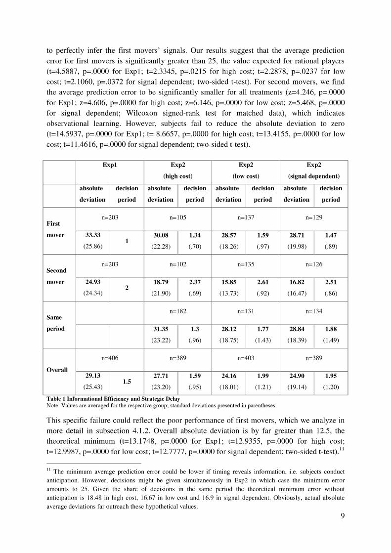
to perfectly infer the first movers’ signals. Our results suggest that the average prediction

error for first movers is significantly greater than 25, the value expected for rational players

(t=4.5887, p=.0000 for Exp1; t=2.3345, p=.0215 for high cost; t=2.2878, p=.0237 for low

cost; t=2.1060, p=.0372 for signal dependent; two-sided t-test). For second movers, we find

the average prediction error to be significantly smaller for all treatments (z=4.246, p=.0000

for Exp1; z=4.606, p=.0000 for high cost; z=6.146, p=.0000 for low cost; z=5.468, p=.0000

for signal dependent; Wilcoxon signed-rank test for matched data), which indicates

observational learning. However, subjects fail to reduce the absolute deviation to zero

(t=14.5937, p=.0000 for Exp1; t= 8.6657, p=.0000 for high cost; t=13.4155, p=.0000 for low

cost; t=11.4616, p=.0000 for signal dependent; two-sided t-test).

Exp1 Exp2

(high cost)

Exp2

(low cost)

Exp2

(signal dependent)

absolute

deviation

decision

period

absolute

deviation

decision

period

absolute

deviation

decision

period

absolute

deviation

decision

period

First

mover

n=203 n=105 n=137 n=129

33.33

(25.86) 1

30.08

(22.28)

1.34

(.70)

28.57

(18.26)

1.59

(.97)

28.71

(19.98)

1.47

(.89)

Second

mover

n=203 n=102 n=135 n=126

24.93

(24.34) 2

18.79

(21.90)

2.37

(.69)

15.85

(13.73)

2.61

(.92)

16.82

(16.47)

2.51

(.86)

Same

period

n=182 n=131 n=134

31.35

(23.22)

1.3

(.96)

28.12

(18.75)

1.77

(1.43)

28.84

(18.39)

1.88

(1.49)

Overall

n=406 n=389 n=403 n=389

29.13

(25.43) 1.5

27.71

(23.20)

1.59

(.95)

24.16

(18.01)

1.99

(1.21)

24.90

(19.14)

1.95

(1.20)

Table 1 Informational Efficiency and Strategic Delay Note: Values are averaged for the respective group; standard deviations presented in parentheses.

This specific failure could reflect the poor performance of first movers, which we analyze in

more detail in subsection 4.1.2. Overall absolute deviation is by far greater than 12.5, the

theoretical minimum (t=13.1748, p=.0000 for Exp1; t=12.9355, p=.0000 for high cost;

t=12.9987, p=.0000 for low cost; t=12.7777, p=.0000 for signal dependent; two-sided t-test).11

11

The minimum average prediction error could be lower if timing reveals information, i.e. subjects conduct

anticipation. However, decisions might be given simultaneously in Exp2 in which case the minimum error

amounts to 25. Given the share of decisions in the same period the theoretical minimum error without

anticipation is 18.48 in high cost, 16.67 in low cost and 16.9 in signal dependent. Obviously, actual absolute

average deviations far outreach these hypothetical values.

10

Comparing the experiments, Exp1 and Exp2 differ, as second movers in Exp2 show

significantly higher prediction accuracy (z=3.685, p=0.0002; Mann-Whitney U-Test), and

thus the overall efficiency is higher. There is no significant difference for first movers

(z=1.255, p=0.2094; Mann-Whitney U-Test).

When comparing the endogenous treatments to Exp1, the data might indicate a better

performance of first movers in low cost and signal dependent. The average absolute deviation

in Exp1 is about 17% (19%) higher compared to low cost (signal dependent). Note, however,

that there are no differences measured by the absolute deviations at the conventional levels of

significance (z=0.637, p=.5239 for high cost; z=1.361, p=.1734 for low cost; z=1.210,

p=.2261 for signal dependent; Mann-Whitney U-Test). For second movers, the average

prediction error is significantly lower in contrast to Exp1 (z=2.190, p=.0285 for high cost;

z=3.185, p=.0014 for low cost; z=2.960, p=.0031 for signal dependent; Mann-Whitney U-

Test). Even though there are no significant differences in first movers’ performance across experiments, this result might partly be driven by the on average weaker performance of first

movers in Exp1.

Despite the better performance of second movers, we only find a positive and significant net

effect on informational efficiency in low cost (z=0.339, p=.7346 for high cost; z=1.760,

p=.0784 for low cost; z=1.468, p=.142 for signal dependent; Mann-Whitney U-Test) when

considering overall performance. This is clearly due to the large number of simultaneous

decisions, which preclude observational learning. 37.56% of subjects in Exp2 decided

simultaneously (46.4% in high cost, 32.5% in low cost, 34.2% in signal dependent). Thus we

conclude, that, on the one hand, endogenous ordering increases overall informational

efficiency by improved observational learning. On the other, allowing for simultaneous

decisions might fully compensate this effect or even reverse the results in an extreme

scenario.

It is interesting to take a closer look on the distribution of rationality. Therefore, we define

decisions as being rational if prediction value does not deviate from the optimal value derived

by solving the equations in the theoretical framework by more than 5 points (equal to the

width of each payoff interval) in absolute terms. If second mover i follows a non-optimal

prediction, her decision is assumed to be rational if the prediction value falls into the interval

[mi,mi+100], which can be considered a rather lax criterion. The cumulative distribution of

subjects giving rational decisions shows that around 25.9% (11.8%) decide rationally in one

or less projects of Exp1 (Exp2). Moreover, around 79% (56%) do not reach more than three

rational predictions, while 3.5% give more than 4 rational predictions in Exp1, and 10% in

Exp2. We also apply a Fisher exact test, which shows a statistically significant relationship

between the number of rational predictions and the ordering regime (Fisher’s exact=0.003). The differences between Exp1 and Exp2 regarding prediction accuracy are mirrored by

differences in the number of rational predictions. Considering the relationship between the

treatments of Exp2 and the number of rational predictions, we obtain significant results

(Fisher’s exact=0.55). Furthermore, we test for learning effects by running a Skillings-Mack (SM) test for the

differences of the absolute prediction errors over projects. For all the treatments, we find no

11

significant differences.12

However, it is to note that we find some predictions showing a weak

or even a misunderstanding of the game, i.e. subjects expecting the co-player’s signal to be 0, negative or greater than 100. According to this definition there are 38 outliers (9.36% of all

predictions) in Exp1; 15.52% in the first project, 10.34% in the second and 7.93% in later

projects, a decrease that might point to some learning effects. For the treatments of Exp2, we

find fewer predictions characterized by a weak understanding of the game (4.34% of all

predictions for high cost, 3.2% in low cost and 2.55% in signal dependent).

To summarize, we find increases in informational efficiency for endogenous timing when

decisions are not taken simultaneously. Interestingly, our results point to a better performance

of first movers for low cost and signal dependent, though differences are not significant. This

result might be understood as evidence for anticipation effects that require both players in a

decision pair to follow a similar strategy where timing depends on signal strength. However,

this intuition is somewhat misleading: we show in the next subsection that, besides some

evidence for anticipation in Exp2, there is a systematic deviation from rational behavior of

first movers driving the results in Exp1.

After considering first movers’ behavior, we turn to the second movers to investigate whether

weak observational learning and differences between the experiments merely reflect the

poorer performance of first movers.

4.1.1 FIRST MOVER PERFORMANCE

In order to understand the performance of first movers in detail, we test whether expectations

of the co-player’s signals are derived rationally as proposed by Eq.1. We find that the average

expectation (= prediction value – signal) of a co-player’s signal for Exp1 and high cost is 41.3

and 46.6 respectively and thus significantly smaller than the rational value of 50=E(M). For

low cost (49.0) and signal dependent (48.9), there is no such significant deviation from 50 on

average (t=-4.5698, p=.0000 for Exp1; t=-2.4291, p=.0158 for high cost; t=-0.7831, p=.4342

for low cost; t=-0.9725, p=.3317 for signal dependent; two-sided t-test).13

We check for anticipation effects as a way of improving prediction accuracy. We define

anticipation as the systematic adjustment of predictions in response to the decision period of

the co-player. If anticipation is present, the co-player’s decision period should have a

significant effect on prediction values. We find anticipation effects for signal dependent

which can be best shown by considering Figure 1.

12

We apply a Skillings-Mack (SM) test since we have repeated measures given by the predictions of the

participants and also missing values when participants did not give a prediction in a project. For Exp1 we find

(SM=9.933, p(no-ties)=0.1275 and empirical p(ties)~0.1280); for high cost (SM=4.004, p(no-ties)=0.6761 and

empirical p(ties)~0.658); for low cost (SM=6.048, p(no-ties)=0.4178 and empirical p(ties)~0.421) and for signal

dependent (SM=4.504, p(no-ties)=0.06088 and empirical p(ties)~0.585). 13

These results are partially driven by the outliers mentioned; therefore, we tested for the differences after taking

out these values. However, we find the same significant effects (average expectation for Exp1 is 45.0 with t=-

3.7452 and p=.0002; average expectation for high cost is 47.4 with t=-2.3252 and p=.0208; two-sided t-test).

12

Figure 1 Performance of first movers

Figure 1 presents the development of the mean absolute deviation, the mean expectation of

the co-player’s signal and the actual mean of the co-player’s signal over periods.

As the graph for signal dependent shows, first movers correctly expect decreasing signal

strengths over decision periods. Simply assuming the co-player’s signals to be 50 would yield higher prediction errors in later periods. To establish this result, we estimate a model with the

randomly determined signals as the dependent variable and decision period as the explanatory

variable for each treatment.14

Signal strength is estimated to decrease significantly by around

7.9 points per period in signal dependent (t=-8.48; p=.0000), with the respective constant

amounting to 66.88 points.15

The basic requirement for anticipation is fulfilled, i.e. decision

periods reveal information about signal strength. To check whether this additional information

is used, we turn to the player’s expectations of their co-player’s signal conditional on the

decision period. Expectations of the co-player’s signal are estimated to decrease significantly

by 4.3 points per period (t=-5.52; p=.001) in signal dependent; the regression shows a

14

We run a pooled OLS regression applying robust Driscoll and Kraay standard errors. Hence, we control for

unobservable heterogeneity, heteroskedasticity, serial correlation in the idiosyncratic errors of order (2) and

cross-sectional dependence. 15

For high cost the marginal effect of an additional period is estimated to reduce signal strength by -2.9 with a

constant of 56.6. The effects is not significant (t=-1.65; p=.151). For low cost the coefficient is 2.55 and

significant at the 5% level (t=2.85; p=.021), while the constant is 50. Applying fixed effects procedure also

yields a significant decrease of signal strength estimated to be -6.56 points per period in high cost. For the other

treatments results change only slightly.

20

30

40

50

60

70

1 2 3 4 5 1 2 3 4 5 1 2 3 4 5

high cost low cost signal dependent

absolute deviation signal expected signal co-player

decision period

13

constant of 56 points.16

Mirrored by decreasing prediction values over periods, anticipation

thus improves, though not perfectly, prediction accuracy compared to the routine of expecting

50 for the co-player’s signal in signal dependent. It remains unclear whether anticipation only

occurs due to the less complex design of waiting cost in signal dependent or the weighing of

time bonus in between low and high cost. However, we do not find anticipation for low cost

and high cost. Signal strength slightly increases over periods in low cost, whereas

expectations on co-player’s signals do not change. In high cost signal strength significantly

decreases over decision periods; however, again the additional information is not reflected in

player’s expectations.

We conclude that the better performance of first movers in low cost and signal dependent can

be best explained by the occurrence of a systematic downward bias of expectations by first

movers in Exp1 and high cost. We additionally find anticipation for signal dependent, which

improves prediction accuracy compared to the rational routine of expecting 50 as the co-

player’s signal.

4.1.2 SECOND MOVER PERFORMANCE

We now turn to the question of whether the poor performance of first movers is responsible

for inefficient observational learning. Therefore, analogously to the previous analysis for the

first movers, we consider the optimal routine described in Eq.2 in our theoretical framework.

Recall that the optimal response for second movers when assuming rational behavior and no

anticipation of first movers is given by z*|t=2= [z*|t=1 - E(M)] + mi= m1+m2= w; whereby t

indicates the position in the decision sequence. We have already shown that predictions on

average are not perfect. However, perfect predictions by second movers can only be obtained

when first movers follow the rational routine described in Eq.1. Accordingly, we only

consider observations for second movers that follow potentially rational predictions by the

respective first movers. This applies to decisions following predictions that are equal or

greater than 51 points (=min{M}+ E(M)) and smaller or equal than 151 points (=max{M}+

E(M)).17

Expectations of second movers should be characterized as perfectly revealing the

first mover’s signals. We thus test whether [z*|t=1 - E(M)] equals the expectation of the second

movers on average. For Exp1 (high cost/low cost/signal dependent), we find the absolute

deviation of the second movers’ expectations from the optimal expectation amounting to

22.94 (12.19/11.46/13.86) on average and thus to be significantly greater than zero (p=.0000

for all treatments; two-sided t-test). The deviation from the optimal expectation is

significantly higher for Exp1 in contrast to the treatments of Exp2 (z=4.453, p=.0000 for high

cost; z=4.853, p=.0000 for low cost; z=3.220, p=.0013 for signal dependent; Mann-Whitney

U-Test).

16

The regression procedure is implemented as before. For high cost, we get a marginal effect of .025 points (t=-

0.02; p=.981) and for low cost the marginal effect is -.133 points (t=-0.25; p=.807), thus both are not significant.

Using fixed effect procedure does not change coefficients substantially and significances remain the same. 17

Note that, for the analysis of second movers, relying solely on decisions following potentially rational

predictions might be problematic. Players in a decision pair might have observed earlier irrational decisions thus

causing project-interdependent assumptions regarding the co-player’s behavior. However, as this keeps the analysis simple and our results in this section are very robust, we refrain from integrating project-interdependent

effects.

14

These results might be too pessimistic for signal dependent, since we have shown that for the

first movers expectations of the co-player’s signal are significantly correlated with decision

periods. Second movers could adjust their calculation of first movers’ signals respectively,

thus outperforming the rule of Eq.2. As shown above, first movers reduce their expectation

toward the co-player’s signal by a rate of 4.3 points per period in the signal dependent.

Therefore, we check whether second movers account for that systematic adjustment. We run a

regression implementing the same routine as before of the second mover’s expectation on

decision period. We find that second movers are somewhat able to adjust for first movers’ anticipation by reducing their own expectation by a rate of 6.2 points per period (t=-6.36;

p=.001) with a constant of 69.6 in signal dependent.18

However, calculating the average of the absolute deviations of second mover expectations

from realized first mover signals, we find a deviation of 25.9 for Exp1, 20.3 for high cost,

16.6 for low cost and 17.7 for signal dependent. Again, this calculation only considers

decisions taken after potentially rational predictions of first movers. If second movers had

strictly followed the rational routine [z*|t=1 - E(M)] to guess the first mover’s signal, the

difference to realized signals for Exp1 would be reduced to 14.4, 13.1 for high cost, 13.9 for

low cost and 13.7 for signal dependent.

We conclude that the non-optimal performance of second movers does not result from the

poor performance of first movers; rather, it is a source of inefficiency in itself. This effect is

strongest for Exp1, thus second movers in Exp2 treatments perform better on average by a

more efficient observational learning. Consequently, c.p. informational efficiency tends to be

higher when timing is endogenous.

We essentially see two driving forces that improve informational efficiency when ordering is

endogenous. Firstly, we would argue that there is a self-selection conditional on the

understanding of the mechanism of observational learning. The rational routine for second

movers is somewhat more complicated to understand, as one has to comprehend the

expectations and potential anticipation of the preceding player. Thus, players with a deeper

level of reasoning tend to decide later and more frequently achieve observational learning.19

While this might explain the superior performance of second movers in Exp2, it does not

explain equal or in tendency even higher levels of rationality for first movers. On the contrary,

if players with a deeper understanding tend to decide as second movers, first movers should

perform even worse due to self-selection in Exp2 as compared to Exp1. Therefore, we would

argue that the level of understanding hinges on the structure of the decision situation. Having

18

Although we showed that expectations of first movers in the high cost are not related to the decision period,

second movers adjust their expectation significantly by a rate of -8.8 points (t=-3.72; p=0.01). Results for low

cost show an insignificant marginal effect of 1.5 points (t=1.01; p=0.352) for decision period on the second

mover’s expectation. The results do not change substantially when we only use decisions of second movers

following potentially rational decisions of first movers or when we use a fixed effects procedure. 19

Therefore, one might consider a level-k approach to define an appropriate model of behavior in our experiment

(Nagel 1995; Stahl and Wilson 1994, 1995; Crawford and Iriberri 2007), thus rationalizing predictions

conditional on the first mover’s assumed depth of reasoning. However, even interdependent expectations regarding the depth of reasoning of the co-player might not explain the differences in informational efficiency

between Exp1 and Exp2. However, an extensive analysis regarding the expectation on the depth of reasoning is

beyond the scope of this paper.

15

subjects decide when to act induces considerations about the advantages and disadvantages of

being the first and second mover. By inducing these reflections about the game itself, subjects

are more likely to realize the relevance of the co-player’s signal. These considerations might add to the level of understanding for both the first and second movers in case of endogenous

ordering, thereby eliciting more rational behavior overall.

4.2 STRATEGIC DELAY

Strategic delay is the central feature of Exp2 (Table 1 also includes the average decision

periods). While an average decision period of 1.5 is predetermined for Exp1, it is 1.84 for

pooled data of Exp2. The subjects react sensitive towards waiting cost: in high cost, decisions

are taken earlier (1.58) compared to low cost (1.99) and signal dependent (1.94). Only 17

predictions are not given in the subsequent period after a co-player has decided, and thus

excessive delay only occurs in 2% of all projects.

On the individual level, distinct strategies regarding timing can be revealed. There are around

16% of participants in Exp2 always predicting in the first round (26.9% in high cost, 12.1% in

low cost and 9% in signal dependent). These participants minimize waiting cost without

trying to gain additional information by outwaiting the co-player. In 81 of the 91 projects with

simultaneous decisions in high cost, predictions are given in the very first period; 46 of 66 in

low cost and 45 of 67 in signal dependent.

In turn, only 4.1% of participants always predict as second mover or in the last period (3.57%

in high cost, 5.17% in low cost and 3.57% in signal dependent). Thus, only few try to

maximize accuracy regardless of signal strength or waiting cost.

Combining the analyses on informational efficiency and strategic delay, we now investigate

the overall effects on social welfare.

4.3 SOCIAL WELFARE

We measure social welfare by aggregate payoffs. To assess welfare effects, we calculate

average waiting cost and accuracy bonuses. Given that waiting costs are manipulated over

treatments of Exp2, we calculate hypothetical waiting cost for Exp1 according to the payoff

structure of the respective Exp2 treatment in order to enable a comparison.

In Exp1 subjects earn on average 708ECU per projects as accuracy reward compared to

slightly higher 719ECU in the high cost. Subjects take decisions relatively early in the high

cost yielding an average time bonus of 886ECU, which is equivalent to average waiting cost

of 117ECU. Applying the same waiting cost structure to Exp1 gives an average time bonus of

924ECU or average waiting cost of 103ECU. Thus, the total expected payoff in a project of

Exp1 is 1632ECU and 1605ECU for the high cost. On aggregate for the whole game (7

projects), this gives a difference of 189ECU or 21 Cent, which is around 2.1% of the average

payoff (excluding show-up fee). Following the same procedure leads to a 126ECU (14Cent)

lower payoff for the low cost game aggregated for seven projects. The signal dependent game

has a lower payoff of 21ECU (2 Cent). Obviously, these differences are of low relevance.

Another way of looking at this result is to exclude same period decisions, as there might be

several real-world situations where simultaneous decisions are highly unlikely, e.g. high

frequency trading in financial markets. When excluding simultaneous decisions from

calculating the averages, effects on social welfare do not change substantially. The largest

16

treatment effect is given for the signal dependent, in which the average increase in total

payoff amounts to 530ECU, which convert to 58 Cent or 5.9% of average payoff (for high

cost difference amounts to -13ECU and for low cost to 25ECU).

Overall, gains in informational efficiency are realized at the expense of increased waiting

cost, such that no relevant effects on social welfare are elicited by introducing endogenous

ordering. In the given gambling structure, waiting cost and informational efficiency turn out

to be strongly interdependent, causing the absence of net effects on social welfare. Placing

different relative weights on waiting cost shows no influence on social welfare, given that

participants adjust their timing of decisions accordingly.

5. CONCLUDING REMARKS

The present study investigates informational efficiency in a game of social learning,

comparing exogenous and endogenous ordering of choices. By quantifying the effect of

observational learning and waiting cost, we show the welfare effects of these different

regimes of ordering. Based on the model by Gul and Lundholm (1995), we run a two-player

prediction game with a benchmark treatment of exogenous ordering and three treatments of

endogenous ordering. Rather than the classic binary action sets following the seminal

Anderson and Holt (1997) paper, we introduce a continuous action space to more precisely

determine the success of observational learning. We refrain from implementing an optimal

timing conditional on signal strength to expose subjects to a situation where gambling on the

co-player’s uncertain action is required. We argue that both the continuous action space and

gambling situation that our subjects faced depict actual decisions in social learning

environments more closely than the informational cascade games characterized by binary

decisions and exogenous ordering.

In our treatments, endogenous timing enhances the rationality of predictions and thus their

accuracy, yet also leads to higher waiting cost. Subjects react sensitively to changes in waiting

cost and adjust their timing accordingly. This leads to earlier and often simultaneous decisions

that inhibit observational learning. For lower waiting cost, subjects tend to wait longer, which

fosters observational learning, yet increases waiting cost to the same degree. Thus, there are

no overall positive welfare effects in our endogenous treatments. However, despite the

specific incentive to always outwait the co-player, we rarely find war of attrition situations

that would massively reduce welfare. We suggest that making subjects take a timing decision

in the endogenous game fosters a deeper level of reasoning in general, which leads to a more

efficient observational learning. Additionally, observational learning might be improved by a

self-selection according to the understanding of second mover advantages. Our results show

that introducing an endogenous rather than exogenous ordering regime leads to higher

informational efficiency but does not increase overall social welfare.

We add to the literature on social learning by introducing an experiment that enables

comparison between exogenous and endogenous ordering of choices. This allows us to

combine the discussions following the seminal urn experiment by Anderson and Holt (1997)

with the studies on endogenous ordering following Sgroi (2003). Both strands of literature

investigate the success of social learning and informational efficiency, yet fail to compare the

two settings. We qualify the extent of informational efficiency in a unitary setting across

regimes of ordering. While informational efficiency is effectively increased with the

17

introduction of endogenous ordering, as suggested by previous studies, we cannot conclude

that this leads to a positive effect on social welfare. However, it also does not deteriorate

welfare altogether, as situations with extreme waiting cost are rare. Our results suggest that

social learning is fairly effective when implementing a continuous action space and

endogenous timing. Therefore, the informational inefficiency in situations of rational herding

emphasized by numerous studies is limited to specific decision situations and should not be

generalized.

18

Your Information + Co-player’s Information = Project value

(1 to 100) (1 to 100) (2 to 200)

Example: 25 + 50 = 75

APPENDIX

Instructions for Experiment 1

The Game

In this game you and a co-player will estimate the value of a project. The value of the project

consists of two parts: your own information and your co-player’s information. Your information and the information of your co-player are randomly determined numbers

between 1 and 100. Therefore, project value that you have to estimate is always between 2

and 200. All of the possible information is equally likely.

There are 7 projects in which you will estimate the project value. In every project, it will be

randomly determined if you or your co-player will give the estimation first. The first

estimation is always displayed to the other player. Once both players have made their

estimation, the next project begins.

You will have the same co-player in all projects. You have a maximum of one minute for

each estimation. If you do not type in an estimation in time, you will not receive a payoff for

this project!

The payoff

You will receive a precision bonus in every project, which depends on how precise your

estimation was. The precision bonus depends on the deviation of your estimation from the

correct project value. 1000 ECU equals a payoff of 1.70€. Additionally, you will receive an

independent payoff of 2.50€. The following table clarifies the precision bonus:

Distance from correct

project value

Precision bonus

(in ECU)

Example: The project value is 100.

Your estimation

was… The precision bonus is…

0 – 5 points 2000 …96 …2000 ECU

6 – 10 points 1600 …109 …1600 ECU

11 – 15 points 1200 …87 …1200 ECU

16 – 20 points 800 …118 …800 ECU

21 – 25 points 400 …75 …400 ECU

from 26 points 0 …12 …0 ECU

19

Example

At the beginning of a project your information is 45. Therefore, you know that the project

value is at least 45 plus the information of your co-player. Your co-player decides before you

and estimates a project value of 120. You decide after him and estimate a project value of

105. The correct project value is 95. Thus, you receive a precision bonus of 1600 ECU, as

your estimation deviated from the correct project value by 10 points.

20

Your Information + Co-player’s Information = Project value

(1 to 100) (1 to 100) (2 to 200)

Example: 25 + 50 = 75

Instructions for Experiment 2.

Note that the instructions refer to the high cost treatment. The differences from the other

treatments are indicated as follows: information in square brackets corresponds to the signal

dependent treatment, braces corresponds to the low cost treatment.

The Game

In this game you and a co-player will estimate the value of a project. The value of the project

consists of two parts: your own information and your co-player’s information. Your information and the information of your co-player are randomly determined numbers

between 1 and 100. Therefore, the project value that you have to estimate, is always between

2 and 200. All of the possible information is equally likely.

There are 7 projects in which you will give an estimation of the project value. All projects

have 5 rounds of 2 minutes each. You must decide in which round you want to give your

estimation.

All projects end once both players have given their estimation. Subsequently, the next project

starts. You will have the same co-player in all projects. The following table provides an

example of the course of the game:

At the beginning of each project, both players receive their information. Your co-player’s information is unknown to you. You will have to decide in every round if you want to give an

estimation (YES/NO). If you allow 2 minutes per round to elapse, you will not get a payoff

for this project! If you choose NO, please wait for the next round of the project. If you choose

YES, you will be told if your co-player will give an estimation in the same round.

Subsequently, you will enter your estimation. Meanwhile, you will see an overview of the last

rounds and, if applicable, the estimation of your co-player. If you decide before your co-

player, your estimation will also be shown to him. The following table exemplifies the course

of the game and your possible actions:

project 1 project 2

round 1 round 2 round 3 round 4 round 5 round 1 …

2 min. 2 Min. 2 min. 2 min. 2 min. 2 min. …

Round 1 Round 2 Round 3 Round 4 Round 5

Action by

Player 1 NO NO NO

YES!

Enters the

estimation Project

completed! Action by

Player 2 NO

YES!

Enters the

estimation

Wait for the co-player…

21

The payoff

The total payoff consists of two parts: the accuracy bonus (I.) and the time bonus (II.). For

every round you wait with your estimation, your time bonus will be reduced. The precision

bonus is higher, the closer your estimation gets to the correct project value. 1000 coins equal a

payoff of 0.80€ {1.20€}, [1.20€]. Additionally, you will receive an independent payoff of

2.50€. I. Precision bonus

You receive a bonus in every project which depends on the precision of your

estimation, based upon its distance to the correct project value. The following table

clarifies the precision bonus:

II. Time bonus

You receive a time bonus in every project, depending on the size of the project

value {on the size of your information}. For every round you wait with your

estimation, your time bonus will be reduced. The following table clarifies the time

bonus:

Distance from the

correct project value

Precision bonus

(in ECU)

Example: The project value is 100.

Your estimation

was… The precision bonus is…

0 – 5 points 2000 …96 …2000 coins

6 – 10 points 1600 …109 …1600 coins

11 – 15 points 1200 …87 …1200 coins

16 – 20 points 800 …118 …800 coins

21 – 25 points 400 …75 …400 coins

ab 26 points 0 …12 …0 coins

Estimation in

round Time bonus

Example: The project value is 100.

Estimation in round… Time bonus…

1

10{5} x project

value [10 x

Information]

…1

…1000{500} ECU

[1000 ECU]

2

8{4} x project

value

[8 x Information]

…2

…800{400} ECU

[800 ECU]

3

6{3} x project

value

[6 x Information]

…3

…600{300} ECU

[600 ECU]

4

4{2} x project

value

[4 x Information]

…4

…400{200} ECU

[400 ECU]

5

2{1} x project

value

[2 x Information]

…5

…200{100} ECU

[200 ECU]

22

Example:

At the beginning of a project, your information is 45. Therefore, you know that the project

value is at least 45 plus the information of your co-player. Your co-player decides before you

and estimates in round 3 that the project value is 120. You decide in round 4 and estimate that

the project value is 105. The correct project value is 95. Therefore, you receive a time bonus

of 380 (time bonus in round 4 = 4 x project value) {190 (time bonus in round 4 = 2 x project

value)} [180 (time bonus in round 4 = 4 x information)]. Additionally, you receive a precision

bonus of 1600 coins, as your estimation deviates from the correct project value by 10 points.

23

REFERENCES

Alevy, J.E., Haigh, M.S., List, J.A., 2007. Information Cascades: Evidence from a Field

Experiment with Financial Market Professionals. Journal of Finance, 62 (1), 151-180. doi:

10.1111/j.1540-6261.2007.01204.

Anderson, L.R., 2001. Payoff Effects in Information Cascade Experiments. Economic Inquiry

39 (4), 609-615. doi: 10.1093/ei/39.4.609.

Anderson, L.R. Holt, C.A., 1997. Information Cascades in the Laboratory. American

Economic Review 87 (5), 847-862.

Banerjee, A.V., 1992. A simple model of herd behavior. Quarterly Journal of Economics 107

(3), 797-817. doi: 10.2307/2118364.

Bikhchandani, S., Hirshleifer, D., Welch, I., 1992. A theory of fads, fashion, custom, and

cultural change in informational cascades. Journal of Political Economy 100 (5), 992-1026.

doi:10.1086/261849.

Çelen, B., Kariv, S., 2004. Distinguishing Informational Cascades from Herd Behavior in the

Laboratory. American Economic Review 94 (3), 484-498. doi: 10.1257/0002828041464461.

Çelen, B., Hyndman, K., 2012. An experiment of social learning with endogenous Timing.

Review of Economic Design 16, 251-268. doi: 10.1007/s10058-012-0127-5.

Chamley, C., 2004. Rational Herds: Economic Models of Social Learning. Cambridge:

Cambridge University Press.

Chamley, C., Gale, D., 1994. Information revelation and strategic delay in a model of

investment. Econometrica 62 (5), 1065-1085.

Cipriani, M., Guarino, A., 2005. Herd Behavior in a Laboratory Financial Market. American

Economic Review 95 (5), 1427-1443. doi: 10.1257/000282805775014443.

Crawford, V.P., Iriberri, N., 2007. Level-k auctions: can a nonequilibrium model of strategic

thinking explain the winner’s curse and overbidding in private-value auctions?. Econometrica

75 (6), 1721-1770. doi: 10.1111/j.1468-0262.2007.00810.x.

Dominitz, J., Hung, A.A., 2009. Empirical Models of Discrete Choice and Belief Updating in

Observational Learning Experiments. Journal of Economic Behavior & Organization 69 (2),

94-109. doi: 10.1016/j.jebo.2007.09.009.

24

Drehmann, M., Oechssler, J., Roider, A., 2005. Herding and Contrarian Behavior in Financial

Markets: An Internet Experiment. American Economic Review 95 (5), 1403-1426. doi:

10.1257/000282805775014317.

Fahr, R., Irlenbusch, B., 2011. Who follows the crowd – Groups or individuals?. Journal of

Economic Behavior & Organization 80, 200-209. doi:10.1016/j.jebo.2011.03.007.

Fischbacher, U., 2007. Z-tree: zurich toolbox for ready-made economic experiments.

Experimental Economics 10 (2), 171-178. doi: 10.1007/s10683-006-9159-4.

Frisell, L., 2003. On the Interplay of Informational Spillovers and Payoff Externalities. The

RAND Journal of Economics 34 (3), 582-592.

Goeree, J.K., Palfrey, T.R., Rogers, B.W., McKelvey, R.D., 2007. Self-correcting information

cascades. Review of Economic Studies 74, 733-762. doi: 10.1111/j.1467-937X.2007.00438.x.

Greiner, B., 2004. An Online Recruitment System for Economic Experiments, in: Kremer, K.,

Macho, V. (Eds.), Forschung und Wissenschaftliches Rechnen 2003, GWDG Bericht 63.

Göttingen: Gesellschaft für Wissenschaftliche Datenverarbeitung, 79-93.

Gul, F., Lundholm, R., 1995. Endogenous Timing and the Clustering of Agents' Decisions.

Journal of Political Economy 103 (5), 1039-1066. doi: 10.1086/262012.

Hung, A.A., Plott, C.R., 2001. Information Cascades: Replication and an Extension to

Majority Rule and Conformity-Rewarding Institutions. American Economic Review 91 (5),

1508-1520. doi: 10.1257/aer.91.5.1508.

Ivanov, A., Levin, D., Peck, J., 2013. Behavioral biases in endogenous-timing herding games:

An experimental study. Journal of Economic Behavior & Organization 87, 25-34. doi:

10.1016/j.jebo.2012.12.001.

Kübler, D., Weizsacker, G., 2004. Limited Depth of Reasoning and Failure of Cascade

Formation in the Laboratory. Review of Economic Studies 71 (2), 425-441. doi:

10.1111/0034-6527.00290.

Lee, I. H., 1993. On the Convergence of Informational Cascades. Journal of Economic Theory

61, 396-411. doi: 10.1006/jeth.1993.1074.

Levin, D., Peck, J., 2008. Investment dynamics with common and private values. Journal of

Economic Theory 143 (1), 114-139. doi: 10.1.1.151.6944.

Nagel, R. 1995. Unraveling in Guessing Games: An Experimental Study. American Economic

Review 85(5), 1313-1326.

25

Nöth, M., Weber, M., 2003. Information Aggregation with Random Ordering: Cascades and

Overconfidence. Economic Journal 113(484), 166-189. doi: 10.1111/1468-297.00091.

Oberhammer, C., Stiehler, A., 2003. Does Cascade Behavior in Information Cascades Reflect

Bayesian Updating?. Max Planck Institute of Economics Papers Strategic Interaction Group

Discussion Paper, 2003-01, 1-19. doi: 10.1.1.13.3143.

Sgroi, D., 2003. The right choice at the right time: a Herding experiment in endogenous time.

Experimental Economics 6, 159-180. doi: 10.1023/A:1025357004821.

Stahl, D.O., Wilson, P.W., 1994. Experimental evidence on players’ models of other players.

Journal of Economic Behavior & Organization 25 (3), 309-327. doi: 10.1016/0167-

2681(94)90103-1.

Stahl, D.O., Wilson, P.W., 1995. On players’ models of other players: theory and

experimental evidence. Games and Economic Behavior 10, 218-254. doi:

10.1006/game.1995.1031.

Weizsäcker, G., 2010. Do we follow others when we should? A simple test of rational

expectations. American Economic Review 100, 2340-2360. doi: 10.1257/aer.100.5.2340.

Willinger, M., Ziegelmeyer, A., 1998. Are More Informed Agents Able to Shatter Information

Cascades in the Lab?, in: Cohendet, P., Llerena, P., Stahn, H., Umbhauer, G. (Eds.), The

Economics of Networks: Interaction and Behaviours, Berlin, Heidelberg: Springer, 291-305.

Zhang, J., 1997. Strategic Delay and the Onset of Investment Cascades. The RAND Journal of

Economics 28 (1), 188-205.

Ziegelmeyer, A., Bracht, J., Koessler, F., Winter, E., 2008. Fragility of Information Cascades:

An Experimental Study Using Elicited Beliefs. Max Planck Institute of Economics Strategic

Interaction Group Discussion Paper, 2008-094. doi: 10.1.1.197.2212.

Ziegelmeyer, A., My, K.B., Vergnaud, J.C., Willinger, M., 2005. Strategic Delay and Rational

Imitation in the Laboratory. Max Planck Institute of Economics Discussion Paper on Strategic

Interaction 2005-35, 1-26.