A Comparison of Accuracy and Computational Efficiency of

Three Pseudospectral Methods

Geoffrey T. Huntington∗

David Benson†

Charles Stark Draper Laboratory

555 Technology Square

Cambridge, MA 02139

Anil V. Rao‡

University of Florida

Gainesville, FL 32611­6250

Abstract

A comparison is made between three pseudospectral methods used to numerically solve op­

timal control problems. In particular, the accuracy of the state, control, and costate obtained

using the Legendre, Radau, and Gauss pseudospectral methods is compared. Three examples with

different degrees of complexity are used to identify key differences between the three methods.

The results of this study indicate that the Radau and Gauss methods are very similar in accuracy,

while both significantly outperform the Legendre method with respect to costate accuracy. Fur­

thermore, it is found that the computational efficiency of the three methods is comparable. Based

on these results and a detailed analysis of the mathematics of each method, a rationale is created

to determine when each method should be implemented to solve optimal control problems.

1 Introduction

Numerical methods for solving optimal control problems fall into two general categories: indirect

methods and direct methods. In an indirect method, the first­order optimality conditions are derived

using the calculus of variations1 and Pontryagin’s minimum principle.2 These optimality conditions

lead to a Hamiltonian boundary­value problem (HBVP) which is then solved numerically to determine

extremal trajectories. In a direct method, the original optimal control problem is transcribed to a

nonlinear programming problem (NLP) which is solved numerically using a well­established optimiza­

tion method. In recent years, direct methods for solving optimal control problems have become

increasingly popular over indirect methods for several reasons. First, when using a direct method it is

unnecessary to derive the (generally quite complex) first­order optimality conditions (i.e. HBVP). Sec­

ond, even in the case where deriving the HBVP is straightforward, solving the HBVP can be extremely

difficult due to the high sensitivity of the Hamiltonian dynamics to unknown boundary conditions.

∗Draper Laboratory Fellow, Ph.D. Candidate, Dept. of Aeronautics and Astronautics, MIT. E­mail: ghunting­

ton@draper.com.†Draper Laboratory Fellow. E­mail: bensonda@alum.mit.edu‡Assistant Professor, Department of Mechanical and Aerospace Engineering, University of Florida, P.O. Box 116250,

Gainesville, FL, 32611. E­mail: anilvrao@ufl.edu. Corresponding Author.

1

Contrariwise, direct methods require much less mathematical derivation and the resulting NLP can be

solved with much greater ease as compared to the HBVP. For these reasons, direct methods are often

the preferred approach for numerically solving complex optimal control problems.3

The category of direct methods is quite broad and encompasses some very different techniques.4

In particular, the choice of what quantities to discretize and how to approximate the continuous­

time dynamics varies widely amongst the different direct methods. Two of the more common direct

methods are control parameterization and state and control parameterization.5 In a control param­

eterization method, the control alone is approximated and the differential equations are solved via

numerical integration. Examples of control parameterization include shooting methods and multiple

shooting methods. In state and control parameterization methods, the state is discretized in the NLP

as well as the control, and the continuous­time differential equations are converted into algebraic

constraints. These constraints are then imposed in the NLP formulation, which avoid the sensitivity

issues of direct shooting methods at the expense of a larger NLP.

In recent years, considerable attention has been focused on a class of state and control parameter­

ization methods called pseudospectral6–8 or orthogonal collocation9,10 methods. In a pseudospectral

method, a finite basis of global interpolating polynomials is used to approximate the state and con­

trol at a set of discretization points. The time derivative of the state in the dynamic equations is

approximated by the derivative of the interpolating polynomial and is then constrained to be equal

to the vector field of the dynamic equations at a set of collocation points. While any set of unique

collocation points can be chosen, generally speaking an orthogonal collocation is chosen, i.e. the col­

location points are chosen to be the roots of an orthogonal polynomial (or linear combinations of

such polynomials and their derivatives). Because pseudospectral methods are generally implemented

via orthogonal collocation, the terms pseudospectral and orthogonal collocation are essentially inter­

changeable (thus researchers in one field use the term pseudospectral8 while others use the term

orthogonal collocation9). One advantage to pseudospectral methods is that for smooth problems,

pseudospectral methods typically have faster convergence rates than other methods, exhibiting so

called “spectral accuracy”.11 For non­smooth problems or problems where modeling changes are

desired, the optimal control problem can be divided into phases and orthogonal collocation can be

applied globally within each phase. A vast amount of work has been done on using pseudospectral

methods to solve non­smooth optimal control problems (see Refs. 12–17).

Pseudospectral methods in optimal control arose from spectral methods which were traditionally

used to solve fluid dynamics problems.7,8 Meanwhile, seminal work in orthogonal collocation meth­

ods in optimal control date back to 1979 with the work of Ref. 18 and some of the first work using

orthogonal collocation methods in engineering can be found in the chemical engineering literature.17

More recent work in chemical and aerospace engineering have used collocation at the Legendre­Gauss­

Radau (LGR) points.19–21 Because the LGR collocation technique has many similarities to other pseu­

dospectral methods, in this paper we adopt the term Radau pseudospectral method (RPM) for LGR

collocation. Within the aerospace engineering community, several well­known pseudospectral meth­

ods have been developed for solving optimal control problems such as the Chebyshev pseudospectral

method (CPM),22,23 the Legendre pseudospectral method (LPM),6 and the Gauss pseudospectral method

(GPM).24 The CPM uses Chebyshev polynomials to approximate the state and control, and performs

orthogonal collocation at the Chebyshev­Gauss­Lobatto (CGL) points. An enhancement to the Cheby­

shev pseudospectral method that uses a Clenshaw­Curtis quadrature was developed in Ref. 30. The

LPM uses Lagrange polynomials for the approximations, and Legendre­Gauss­Lobatto (LGL) points for

the orthogonal collocation. A costate estimation procedure for the Legendre pseudospectral method

was developed by in Ref. 25 and recently updated in Ref. 26. Recent work by Williams shows several

variants of the standard LPM. The Jacobi pseudospectral method27 is a more general pseudospectral

approach that uses Jacobi polynomials to find the collocation points, of which Legendre polynomials

2

are a subset. Another variant, called the Hermite­LGL method,28 uses piecewise cubic polynomials

rather than Lagrange polynomials, and collocates at a subset of the LGL points. These new methods

have not yet become mainstream optimization techniques because of their novelty, but the new soft­

ware tool DIRECT29 could expedite this process. Lastly, in the GPM, the state is approximated using

a basis of Lagrange polynomials similar to the LPM, and the optimal control problem is orthogonally

collocated at the interior Legendre­Gauss (LG) points.

Two key features of these pseudospectral methods is the choice of discretization points and collo­

cation points. Discretization points (or nodes) are the points used to discretize the state and control

that are fed into the nonlinear program. Collocation points are the points used to collocate the dif­

ferential equations to ensure the dynamics have been met. As we will see, these two sets of points

drastically affect the accuracy of the methods. Among the pseudospectral methods previously men­

tioned, a unique quality exists for the Gauss pseudospectral method. The specific choice of colloca­

tion and discretization points in the GPM results in an equivalence between the Karush­Kuhn­Tucker

(KKT) conditions of the NLP and the discretized form of the first­order optimality conditions at the

LG points. In other words, the solution of the NLP (direct approach) also satisfies the same first­order

conditions if one were using an indirect approach.24 A diagram of this equivalence for the GPM is

shown in Fig. 1. Although an exact equivalence has not been proven for the other methods, much

research has been done on both the LPM and the RPM that discusses the (rapid) convergence rates of

the NLP solution to the solution of the continuous­time optimality conditions.19,26,31 Moreover, for

both the LPM and the RPM a relationship between the KKT conditions and the discretized first­order

necessary conditions leads to method for costate approximation based on the KKT multipliers of the

NLP. These costate approximation procedures have been documented for the RPM in Ref. 19, for the

LPM in Ref. 25,26, and for the GPM in Ref. 24. The accuracy of these procedures, as well as the state

and control approximations themselves, are compared in this paper for the GPM, LPM and RPM.

Numerical comparisons between methods are often difficult to perform fairly because many direct

methods are integrated with a specific NLP solver, thereby making it difficult to distinguish between

differences between the methods and differences due to the NLP solvers. This is perhaps why there

are relatively few papers that actually compare the performance of several direct methods. In fact,

even survey papers, such as that found in Ref. 3, stop short of providing comparisons between various

methods. However, some research has been done that compares direct methods. Ref. 32 is primarily

focused on presenting enhanced mesh refinement and scaling strategies, but contains a brief com­

parison of the accuracy of direct implicit integration schemes (like Hermite­Simpson integration) and

pseudospectral methods. Williams created the software tool DIRECT in order to more effectively com­

pare various trajectory optimization algorithms. The results of a thorough comparison involving 21

test problems of several different direct methods is presented in Ref. 29. Ref. 33 presents a com­

parison between several pseudospectral approaches, but uses unorthodox variants of pseudospectral

methods that are inconsistent with a large majority of the literature.

In this paper a comparison is made between the Legendre, Radau, and Gauss pseudospectral meth­

ods. In order to provide a fair comparison, in this study the NLP solver SNOPT39 is used for each

of the discretizations. Furthermore, all three methods are implemented using the same version of

MATLAB R© and the initial guesses provided for all examples are identical. Using this equivalent setup

for all three methods, the goal of the study is to assess the similarities and differences in the accuracy

and and computational performance between the three methods. Three examples are used to make

the comparison. The first two examples are designed to be sufficiently simple so that the key fea­

tures of each method can be identified. The third example, a commonly used problem in aerospace

engineering, is designed to provide an assessment as to how the three methods compare on a more

realistic problem. A great deal of the emphasis of this study is to understand when one method may

perform better than another method and to identify why such an improved performance is attained

3

in such circumstances.

The results of this study indicate that the Radau and Gauss pseudospectral methods are highly

comparable in numerical accuracy, computational efficiency, and ease of use. The largest discrep­

ancy in accuracy between these two methods corresponds to the costate at the final time, where the

natural equivalence in the GPM leads to a more accurate final costate. This study also shows that,

even on simple problems, both the Radau and Gauss methods produce higher accuracy solutions as

compared to the Legendre method. Specifically, the costate estimates obtained using the Radau and

Gauss methods are superior to the costate estimate obtained using the established method of Ref. 25.

The authors recognize that improvements to these methods are still occurring, therefore a second

computation is performed using a recent advancement of the Legendre pseudospectral method. The

augmented set of KKT conditions26 is solved using the Legendre method with the covector mapping

theorem, and the resulting costate is compared with the Radau and the Gauss methods. While it is

found that this new costate is significantly more accurate than the original costate obtained using the

method of Ref. 25, it still does not provide costate accuracies comparable to the GPM and RPM for

a given number of discretization points. Furthermore, it is argued that such an approach is highly

intractable because it requires formulating a primal­dual problem involving the transversality condi­

tions of the HBVP and the (generally quite complex) KKT conditions of the NLP, thus defeating the

purpose of costate estimation using the solution from a direct method.

The increased accuracy in the Radau and Gauss costates arises from the fact that no collocation

occurs at least one of the endpoints in these two methods. As a result, the conflict26 that arises in the

Legendre method between the transversality conditions and the discretized dynamics and quadrature

approximation is eliminated or mitigated. The results of this study suggest that the Gauss method

produces the most accurate costate estimates, followed closely by the Radau method. Depending on

the costate approximation procedure chosen for the Legendre method, it produces either a signifi­

cantly less accurate costate, or requires relatively much more computational expense than either the

Radau or Gauss approach.

2 Continuous Mayer Problem

Without loss of generality, consider the following optimal control problem in Mayer form. Determine

the state, x(τ) ∈ Rn, and control, u(τ) ∈ Rm, that minimize the cost functional

J = Φ(x(τf )) (1)

subject to the constraintsdx

dτ=tf − t0

2f(x(τ),u(τ)) ∈ Rn (2)

φ(x(τ0),x(τf )) = 0 ∈ Rq (3)

The optimal control problem of Eqs. (1)–(3) will be referred to as the continuous Mayer problem. It

is noted that, in order to simplify the computational expense and provide a clear comparison, we

consider optimal control problems with fixed terminal times and without algebraic path constraints.

Furthermore, it is noted that the time interval τ ∈ [−1,1] can be transformed to the the time interval

t ∈ [t0, tf ] via the affine transformation

t =tf − t0

2τ +

tf + t0

2(4)

4

3 First­Order Necessary Conditions of Continuous Mayer Problem

The indirect approach to solving the continuous Mayer problem of Eqs. (1)–(3) in Section 2 is to

apply the calculus of variations and Pontryagin’s Minimum Principle2 to obtain first­order necessary

conditions for optimality.1 These variational conditions are typically derived using the Hamiltonian,

H , defined as

H (x,λ,u) = λT f(x,u) (5)

where λ(τ) ∈ Rn is the costate. Note that, for brevity, the explicit dependence of the state, control,

and costate on τ has been dropped. Assuming that the optimal control lies interior to the feasible

control set, the continuous­time first­order optimality conditions are

dx

dτ=

tf − t0

2f(x,u) =

tf − t0

2

∂H

∂λ

dλ

dτ= −

tf − t0

2λT∂f

∂x= −

tf − t0

2

∂H

∂x

0 = λT∂f

∂u=

∂H

∂u

φ(x(τ0),x(τf )) = 0

λ(τ0) = νT∂φ

∂x(τ0), λ(τf ) =

∂Φ

∂x(τf )− νT

∂φ

∂x(τf )

(6)

where ν ∈ Rq is Lagrange multiplier associated with the boundary condition φ. The optimality

conditions of Eq. (6) define a Hamiltonian boundary value problem (HBVP).

4 Pseudospectral Approximation Methods

Before proceeding to the comparison, it is important to understand the mathematics associated with

each pseudospectral method. This section provides an overview of the mathematics implemented in

the different methods and highlights the key differences.

4.1 Global Polynomial Approximations

All three pseudospectral methods compared in this paper (i.e. Legendre, Radau, and Gauss) employ

global polynomial approximations using Lagrange interpolating polynomials as the basis functions.

These polynomials are defined using a set of N support points τ1, . . . , τN on the time interval τ ∈[−1,1]. The state, control, and costate of the optimal control problem are all approximated as35

y(τ) ≈ Y(τ) =N∑

i=1

Li(τ)Y(τi), where Li(τ) =N∏

j=1,j≠i

τ − τjτi − τj

(7)

where Li(τ), (i = 1, . . . , N) is the set of Lagrange interpolating polynomials corresponding to the

chosen support points and Y represents either the state, control, or costate. It can be shown that

Li(τj) =

{

1 , i = j0 , i ≠ j

(8)

Eq. (8) leads to the property that y(τj) = Y(τj), (j = 1, . . . , N), i.e. the function approximation is

equal to the true function at the N points. It is important to keep in mind that the support points

5

are different for each of the three pseudospectral methods. Furthermore, within a given method, the

number of points used in Eq. (7) can be different for each variable (e.g. the state may be approximated

with one basis of Lagrange polynomials, while the control is approximated with a different basis of

Lagrange polynomials). See Table 1 for a complete list of the Lagrange polynomial approximations

used in this paper.

4.2 Quadrature Approximation

In addition to the approximation of the state, control, and costate, each method uses a specific set

of support points at which to collocate the dynamics. These support points are chosen to minimize

the error in the quadrature approximation36 to an integral of a function. The general form for the

quadrature approximation in these pseudospectral methods is

∫ b

af(τ)dτ ≈

N∑

i=1

wif(τi) (9)

where τ1, . . . , τN are the support points of the quadrature on the interval τ ∈ [−1,1] and wi, (i =1, . . . , N) are quadrature weights. For an arbitrary set of unique points τ1, . . . , τN , the quadrature

approximation is exact for polynomials of degree N − 1 or less. However, by appropriately choosing

the support points, the accuracy of the quadrature can be improved greatly. It is well­known that the

quadrature approximation with the highest accuracy for a given number of support points N is the

Gauss quadrature. In particular, the Gauss quadrature is exact for all polynomials of degree 2N−1 or

less. In a Gauss quadrature, the N support points are the Legendre­Gauss (LG) points and are the roots

of the Nth­degree Legendre polynomial, denoted PN(t). These nonuniform support points are located

on the interior of the interval [−1,1], and are clustered towards the boundaries. The corresponding

Gauss quadrature weights are then found by the formula

wi =2

(1− τ2i )[

PN(τi)]2, (i = 1, . . . , N) (10)

where PN is the derivative of the Nth­degree Legendre polynomial.

As we will see, another approach is to use Legendre­Gauss­Radau (LGR) points, which lie on the

interval τ ∈ [−1,1). By forcing a support point to lie at the boundary, the degree of freedom is

reduced by one, thus making this choice of support points accurate to 2N­2. The N LGR points are

defined as the roots of PN(τ)+ PN−1(τ), or the summation of the Nth and (N − 1)th order Legendre

polynomials. The corresponding weights for the LGR points are

w1 =2

N2,

wi =1

(1− τi)[PN−1(τi)]2, i = 2, . . . , N

(11)

The standard set of LGR points includes the initial point but not the final point. This set of LGR

points works well for infinite horizon problems.33 For finite­horizon problems, the LGR points (and

corresponding weights) are often flipped on the interval,21 meaning the set includes the final point

but not the initial point (τ ∈ (−1,1]). This set of LGR points can be found from the roots of PN(τ)−PN−1(τ).

The third set of support points implemented in this paper are the Legendre­Gauss­Lobatto (LGL)

points, which lie on the interval τ ∈ [−1,1]. In this approach, quadrature points are forced to lie

6

at both boundaries, reducing the degree of freedom by an additional one degree, thus making this

quadrature scheme accurate to 2N­3. The N LGL nodes are the roots of (1 − τ2)PN−1(τ) (where

PN−1(τ) is the derivative of the (N − 1)th order Legendre polynomial, PN−1(τ)). The corresponding

weights for the LGL points are

wi =2

N(N − 1)

1

[PN−1(τi)]2, (i = 1, . . . , N) (12)

The mathematics of function approximation and quadrature approximation described in this section

will be used in the formulation of all the pseudospectral methods presented in this paper.

5 Pseudospectral Methods

The three pseudospectral methods in this comparison approximate the state and control using a finite

basis of global polynomials, which are created by first discretizing the problem into N nodes along the

trajectory (described in Section 4). However, the location of these nodes is unique to each method,

along with the choice of basis polynomials. These differences are explained in detail in this section.

Furthermore, all pseudospectral methods transcribe the dynamic equations into algebraic conditions,

which are evaluated at a set of collocation points. These collocation points are also unique to each

method and may or may not be the same as the nodes. The locations of nodes and collocation points,

as well as the choice of basis functions are key features that distinguish these methods from each

other. There are many different types of pseudospectral methods, but this work will be limited to

three methods: the Legendre, Radau, and Gauss pseudospectral methods, since these are the three

methods with published costate approximation procedures. Lastly, it is noted that the indexing in

this section may be slightly different than the indexing contained in the references. This is done

in order to create some commonality between the three methods in terms of their indices, and to

create NLPs that are equivalent in size. Therefore, in all methods, N represents the total number

of discretization points (nodes) used in the NLP resulting from each pseudospectral discretization.

Moreover, in general, the index j will be used to represent the j­th node, while the index k will be

used to represent the k­th collocation point.

5.1 Legendre Pseudospectral Method (LPM)

The Legendre pseudospectral method (LPM), like all pseudospectral methods, is based on approximat­

ing the state using a finite set of interpolating polynomials. The state is approximated using a basis

of N Lagrange interpolating polynomials, Li(τ) (i = 1, . . . , N), as defined in Eq. (7).

x(τ) ≈ X(τ) =N∑

i=1

Li(τ)X(τi) (13)

In the LPM, the location of N nodes are described by the Legendre­Gauss­Lobatto (LGL) points on the

interval τ ∈ [−1,1]. Recall that the endpoints −1 and 1 are included as nodes.

Next, all pseudospectral methods transcribe the dynamic equations by “collocating” the derivative

of this state approximation with the vector field, f(x,u), at a set of points along the interval. Let us

assume there are K points, which we call collocation points. In the LPM, the LGL points are both the

nodes and the points used to collocate the dynamics, meaning N = K. Mathematically, the derivative

of the state approximation at the k­th LGL point, τk, is

x(τk) ≈ X(τk) =N∑

i=1

Li(τk)X(τi) =N∑

i=1

DkiX(τk), (k = 1, . . . , K) (14)

7

where the differentiation matrix, D ∈ RK×N , is defined as

Dki =

PN−1(τk)PN−1(τi)

1τk−τi

, if k ≠ i

− (N−1)N4 , if k = i = 1

(N−1)N4 , if k = i = N

0, otherwise

(15)

The continuous dynamics of Eq. (2) are then transcribed into the following set ofN algebraic equations

via collocation:N∑

i=1

DkiX(τi)−tf − t0

2f(X(τk),U(τk)) = 0, (k = 1, . . . , K) (16)

The approximated control, U(τ), is defined in a similar manner as the state:

u(τ) ≈ U(τ) =N∑

i=1

Li(τ)U(τi) (17)

where τi, i = 1, . . . , N are again the LGL nodes. Again, we emphasize that in the LPM, the LGL points

are both the discretization points and the collocation points. We will see in other methods that these

two sets of points are not the same.

Next, the continuous cost function of Eq. (1) is approximated simply as

J = Φ(X(τN)) (18)

Lastly, the boundary constraint of Eq. (3) is expressed as

φ(X(τ1),X(τN)) = 0 (19)

The cost function of Eq. (18) and the algebraic constraints of Eqs. (16) and (19) define an NLP whose

solution is an approximate solution to the continuous Mayer problem. Finally, it is noted that discon­

tinuities in the state or control can be handled efficiently by dividing the trajectory into phases, where

the dynamics are transcribed within each phase and then connected together by additional phase

interface (a.k.a linkage) constraints.16

5.2 Radau Pseudospectral Method (RPM)

The Radau pseudospectral method has been primarily used in the chemical engineering community.

The location of the nodes in the Radau method are based on the flipped Legendre­Gauss­Radau (LGR)

points, which lie on the interval τ ∈ (−1,1]. Recall that this set of points includes the final point but

not the initial point. When discretizing optimal control problems, it is desirable that the discretization

span the entire interval, including both endpoints. Therefore, in order to complete the full discretiza­

tion of the time interval, the N discretization points are found using N − 1 flipped Radau points plus

the initial point, τ0 ≡ −1. The state approximation is constructed exactly the same as the Legendre

pseudospectral method, using a basis of N Lagrange polynomials:

x(τ) ≈ X(τ) =N−1∑

i=0

Li(τ)X(τi) (20)

where we make a slight index modification from (i = 1, . . . , N) used in the LPM to (i = 0, . . . , N − 1).

This new index highlights the fact that the nodes τi, i = 0, . . . , N − 1 are the initial point plus the N­1

LGR points.

8

Unlike the Legendre pseudospectral method, the Radau method uses a different number of col­

location points, K, than discretization points, N. Specifically, the collocation points are the N − 1

LGR points, while the discretization points are the LGR points plus the initial point, τ0. Therefore,

K = N − 1. The K collocation equations are then described as

K∑

i=0

Li(τk)X(τi)−tf − t0

2f(X(τk),U(τk)) = 0, (k = 1, . . . , K) (21)

where τk are the LGR points and

Li(τk) = Dki =

g(τk)

(τk − τi)g(τi), if k ≠ i

g(τi)

2g(τi), if k = i

(22)

where the function g(τi) = (1+τi)[PK(τi)−PK−1(τi)] and τi, (i = 0, . . . , K) are the K LGR points plus

the initial point. Since the collocation equations involve the control solely at the Radau points, the

control is approximated using N − 1 Lagrange polynomials, Lk(τ) (k = 1, . . . , N − 1), as

u(τ) ≈ U(τ) =N−1∑

k=1

Lk(τ)U(τk) (23)

where τk again are the LGR points. This control approximation uses one less point than the state

approximation meaning there is no control defined at the initial point. See Table 1 for more details.

In practice, the initial control is simply extrapolated from Eq. (23). The discretization of the rest of the

optimal control problem is similar to the LPM. The continuous cost function of Eq. (1) is approximated

as

J = Φ(X(τK)) (24)

Recall that in the Radau method, the final LGR point τK = 1. Lastly, the boundary constraint of Eq. (3)

is expressed as a function of the initial point and the final point as

φ(X(τ0),X(τK)) = 0 (25)

The cost function of Eq. (24) and the algebraic constraints of Eqs. (21) and (25) define an NLP whose

solution is an approximate solution to the continuous Mayer problem. As with the LPM, discontinuities

in the state or control can be handled efficiently by dividing the trajectory into phases. In fact, in the

chemical engineering community, it is common practice to break the trajectory up into many phases

and use relatively few numbers of collocation points in each phase.19

5.3 Gauss Pseudospectral Method (GPM)

The location of the nodes in the Gauss pseudospectral method are based on Legendre­Gauss (LG)

points, which lie on the interval τ ∈ (−1,1). This set of points includes neither the initial point nor

the final point. Therefore, in order to fully discretize the time interval, the N discretization points

are (N − 2) interior LG points, the initial point, τ0 ≡ −1, and the final point, τF ≡ 1. The state is

approximated using a basis of N­1 Lagrange interpolating polynomials, which is slightly smaller than

the previous two methods,

x(τ) ≈ X(τ) =N−2∑

i=0

Li(τ)X(τi) (26)

9

where τi (i = 0, . . . , N − 2) are the initial point plus the (N − 2) LG points. Note that the final point,

although it is part of the NLP discretization, is not part of the state approximation. This results in

a state approximation that is one order less than the previous methods, but is necessary in order to

have the equivalence property between the KKT conditions and HBVP conditions. This issue will be

revisited in the results section.

As in the Radau pseudospectral method, the Gauss pseudospectral method uses a different num­

ber of collocation points, K, than discretization points, N. Specifically, the collocation points are

the LG points, while the discretization points are the LG points plus the initial point and final point.

Therefore, K = N − 2. The K collocation equations are then described as

K∑

i=0

DkiX(τi)−tf − t0

2f(X(τk),U(τk)) = 0, (k = 1, . . . , K) (27)

where τk, (k = 1, . . . , K) are the LG points. Note that there is no collocation at either boundary. The

differentiation matrix, D ∈ RK×(N−1), can be determined offline as follows:

Dki = Li(τk) =

(1+ τk)PN(τk)+ PN(τk)

(τk − τi)[

(1+ τi)PN(τi)+ PN(τi)] , i ≠ k

(1+ τi)PN(τi)+ 2PN(τi)

2[

(1+ τi)PN(τi)+ PN(τi)] , i = k

(28)

where τk, (k = 1, . . . , K) are the LG points and τi, (i = 0, . . . , K) are the LG points plus the initial

point. The control is approximated at the (N − 2) collocation points using a basis of (N − 2) Lagrange

interpolating polynomials Li(τ), (i = 1, . . . , N − 2) as

u(τ) ≈ U(τ) =N−2∑

i=1

Li(τ)U(τi) (29)

where τi, (k = 1, . . . , N − 2) are the LG points. Table 1 lists all the Lagrange polynomial expressions

described in this work. Close inspection of Eq. (27) reveals that the collocation equations are indepen­

dent of the final state, X(τF). Therefore, an additional constraint must be added to the discretization

in order to ensure that the the final state obeys the state dynamics. This is enforced by including a

Gauss quadrature to approximate the integral of the dynamics across the entire interval:

X(τF)− X(τ0)−tf − t0

2

K∑

k=1

wkf(X(τk),U(τk)) = 0 (30)

where wk are the Gauss weights and τk are the LG points. Lastly, the cost function is approximated

by

J = Φ(X(τF)) (31)

and the boundary constraint is expressed as

φ(X(τ0),X(τF)) = 0 (32)

The cost function of Eq. (31) and the algebraic constraints of Eqs. (27), (30), and (32) define an NLP

whose solution is an approximate solution to the continuous Mayer problem. The handling of discon­

tinuities in the state or control is explained in the previous two methods.

10

6 Costate Estimate

All three aforementioned pseudospectral methods have an established costate estimation procedure.

In particular, a mapping between the KKT multipliers of the NLP and the costates of the continuous­

time optimal control problem has been derived for all three methods. In this section we describe

these costate estimation procedures which will be implemented later in the paper.

6.1 Legendre Pseudospectral Method

The KKT conditions of the NLP are derived by defining an augmented cost function, which brings the

NLP constraints into the cost function via Lagrange multipliers. For LPM, the augmented cost is

Ja = Φ(XN)− νTφ(X1,XN)−

N∑

k=1

ΛTk

N∑

i=1

DkiXi −tf − t0

2f(Xk,Uk)

(33)

The KKT multipliers in Eq. (33) are Λk, (k = 1, . . . , K), which are associated with the collocation

equations of Eq. (16) and ν, which relates to the boundary condition of Eq. (19). The mapping from

the KKT multipliers to the HBVP variables is:25

Λk =Λk

wk, (k = 1, . . . , K)

ν = ν(34)

The HBVP variables Λk, (k = 1, . . . , N), and ν, now defined in terms of NLP multipliers, can be substi­

tuted into the HBVP equations to determine if the optimality conditions have been met. It has been

documented in the literature26,28 that this mapping for the LPM does not provide an exact equiva­

lence between the KKT conditions and the HBVP conditions. Specifically, the HBVP costate differential

equations are not naturally collocated at the boundaries. In other words, the boundary KKT condi­

tions result in a linear combination of two HBVP conditions: the boundary costate dynamics and the

transversality conditions. We will not derive all the KKT conditions here, but we will present the con­

flicting KKT conditions, which is found by taking the partial derivative of the augmented cost function

with respect to the initial state:

N∑

k=1

ΛkD1k +tf − t0

2Λ1

∂f1

∂X1=

1

w1

(

−Λ1 + νT ∂φ

∂X1

)

(35)

Notice that the left­hand side of the equation resembles the discretized costate dynamics and the

right hand side resembles the transversality condition from the HBVP in Section 3. In order to map

these conditions to the HBVP equations, each side of Eq. (35) should equal zero. However, the two

conditions are inseparable in the LPM. Similarly, the KKT condition corresponding to the final state is

N∑

k=1

ΛkDNk +tf − t0

2ΛN

∂fN

∂XN=

1

wN

(

ΛN −∂Φ

∂XN+ νT

∂φ

∂XN

)

(36)

where again, the left­hand side is the discretized costate dynamics and the right­hand side is the

transversality condition corresponding to the terminal state. It is impossible to get an exact map­

ping from the KKT conditions to the HBVP conditions without being able to separate these mixed

conditions. Recent research26 suggests that by applying relaxation techniques, linear independence

11

constraint qualification, and an additional set of conditions called “closure conditions”, one can show

that there exists a costate approximation that converges to the true costate in the limit. From Ref. 26,

the most recent closure conditions are∥

∥

∥

∥

−Λ∗1 −∂Φ∂x1(X∗1 ,X

∗N)−

(

∂φ∂x1(X∗1 ,X

∗N))Tν∗∥

∥

∥

∥

∞≤ δD

∥

∥

∥

∥

Λ∗N −

∂Φ∂xN

(X∗1 ,X∗N)−

(

∂φ∂xN

(X∗1 ,X∗N))Tν∗∥

∥

∥

∥

∞≤ δD

(37)

where X∗, Λ∗, and ν∗ represent a solution that satisfies Eq. (37) and the KKT conditions, and δDis a dual feasibility tolerance. These conditions are essentially the discretized HBVP transversality

conditions.1 However, it is unclear how the closure conditions are implemented. The covector map­

ping theorem26 states that there exists an N large enough so that the closure conditions and the

KKT conditions will be satisfied to a specified tolerance, δ. Upon close examination of Ref. 26 (and

the references therein) any algorithm attempting to solve the combined KKT conditions and closure

conditions must solve a mixed primal­dual feasibility problem. By including the closure conditions of

Eq. (37) to form the “augmented optimality conditions”, both the state and costate are now variables

to be solved. This procedure significantly increases the computational complexity in finding a costate

approximation. However, both LPM costate approximations (Refs. 25 and 26) are considered in this

paper and their accuracies are compared with the Radau and Gauss methods in the results section.

The LPM costate will be computed first according to Eq. (34), and then by formulating the primal­dual

feasibility problem which attempts to satisfy the augmented KKT conditions according to some toler­

ance, δ. It is noted that improving the LPM costate approximation is an ongoing research topic, and

better methods may be found in the future.

Similar to the LPM state approximate, the continuous­time approximation for the costate is repre­

sented by a basis of N Lagrange interpolating polynomials as

λ(τ) ≈ Λ(τ) =N∑

i=1

Λ(τi)Li(τ) (38)

6.2 Radau Pseudospectral Method

The augmented cost function corresponding to the Radau pseudospectral method is given as

Ja = Φ(XK)− νTφ(X0,XK)−

K∑

k=1

ΛTk

K∑

i=0

DkiXi −tf − t0

2f(Xk,Uk)

(39)

The KKT multipliers resulting from the NLP using the Radau pseudospectral method are Λk, (k =1, . . . , K), associated with the collocation equations of Eq. (21) and ν, associated with the boundary

conditions of Eq. (25). The mapping from the KKT multipliers to the HBVP variables is described as

follows:

Λk =Λk

wk, (k = 1, . . . , K)

ν = ν(40)

The K discrete costates Λk, (k = 1, . . . , K), and the HBVP multiplier ν are now defined in terms of the

KKT multipliers. As in the LPM, it is understood that there is an imperfect match between the KKT

12

multipliers and the costate.21 The Radau method has a similar conflict of HBVP equations when the

partial derivative of the augmented cost function is taken with respect to the final state:

N∑

k=1

ΛkDKk +tf − t0

2ΛK

∂fK

∂XK=

1

wK

(

ΛK −∂Φ

∂XK+ νT

∂φ

∂XK

)

(41)

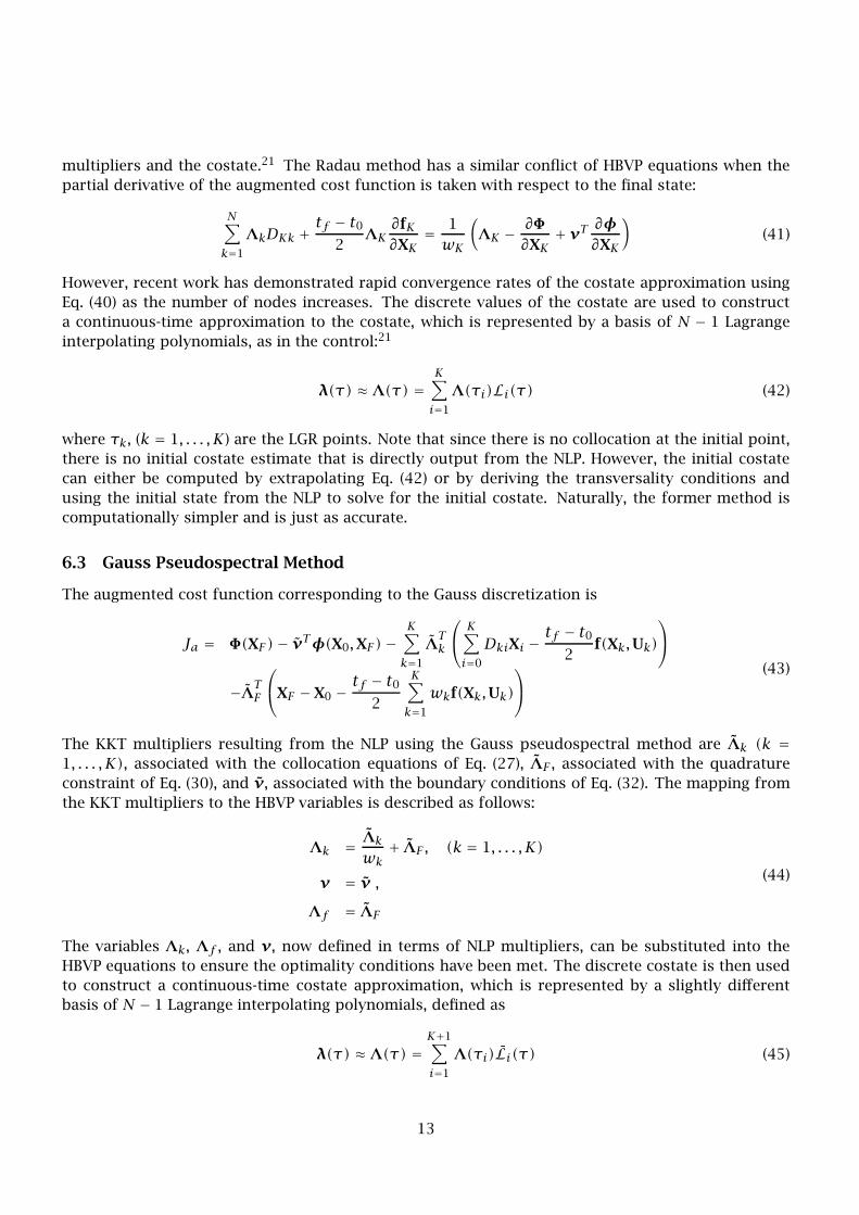
However, recent work has demonstrated rapid convergence rates of the costate approximation using

Eq. (40) as the number of nodes increases. The discrete values of the costate are used to construct

a continuous­time approximation to the costate, which is represented by a basis of N − 1 Lagrange

interpolating polynomials, as in the control:21

λ(τ) ≈ Λ(τ) =K∑

i=1

Λ(τi)Li(τ) (42)

where τk, (k = 1, . . . , K) are the LGR points. Note that since there is no collocation at the initial point,

there is no initial costate estimate that is directly output from the NLP. However, the initial costate

can either be computed by extrapolating Eq. (42) or by deriving the transversality conditions and

using the initial state from the NLP to solve for the initial costate. Naturally, the former method is

computationally simpler and is just as accurate.

6.3 Gauss Pseudospectral Method

The augmented cost function corresponding to the Gauss discretization is

Ja = Φ(XF)− νTφ(X0,XF)−

K∑

k=1

ΛTk

K∑

i=0

DkiXi −tf − t0

2f(Xk,Uk)

−ΛTF

XF − X0 −tf − t0

2

K∑

k=1

wkf(Xk,Uk)

(43)

The KKT multipliers resulting from the NLP using the Gauss pseudospectral method are Λk (k =1, . . . , K), associated with the collocation equations of Eq. (27), ΛF , associated with the quadrature

constraint of Eq. (30), and ν, associated with the boundary conditions of Eq. (32). The mapping from

the KKT multipliers to the HBVP variables is described as follows:

Λk =Λk

wk+ ΛF , (k = 1, . . . , K)

ν = ν ,

Λf = ΛF

(44)

The variables Λk, Λf , and ν, now defined in terms of NLP multipliers, can be substituted into the

HBVP equations to ensure the optimality conditions have been met. The discrete costate is then used

to construct a continuous­time costate approximation, which is represented by a slightly different

basis of N − 1 Lagrange interpolating polynomials, defined as

λ(τ) ≈ Λ(τ) =K+1∑

i=1

Λ(τi)Li(τ) (45)

13

where τi, (i = 1, . . . , K + 1) are the LG points plus the final point, τF . Recall that the state is approx­

imated using (N − 1) Lagrange polynomials based on the LG points and the initial time, while the

costate, λ(τ), is approximated using (N − 1) Lagrange polynomials consisting of the LG points and

the final time. This discrepancy is required to preserve the mapping, and the reader can find more

detailed information in Ref. 24. As in the Radau method, an approximation for the initial costate, Λ0,

cannot be pulled directly from a corresponding multiplier in the NLP because no such multiplier ex­

ists. However, an accurate approximation to the initial costate can be determined from the following

equation:

Λ0 ≡ ΛF −K∑

k=1

Dk0Λk (k = 1, . . . , K) (46)

It is shown in Ref. 38 that this map for the initial costate also satisfies the HBVP transversality condi­

tion

Λ0 = νT ∂φ

∂X0(47)

resulting in a perfect match between the HBVP equations and the KKT conditions. Furthermore, one

could simply extrapolate Eq. (45) to τ0, which would produce an equally accurate initial costate. All

three methods for determining the initial costate are equivalent. The remainder of this paper focuses

on comparing these pseudospectral techniques in terms of their computational efficiency, approxi­

mation accuracy, and solution convergence rates with respect to the state, control, and especially the

costate.

7 Single State Example

As a first example, we consider the following one­dimensional optimal control problem. Minimize the

cost functional

J = −y(tf ) (48)

subject to the constraints

y(t) = y(t)u(t)−y(t)−u2(t) (49)

and the initial condition

y(t0) = 1 (50)

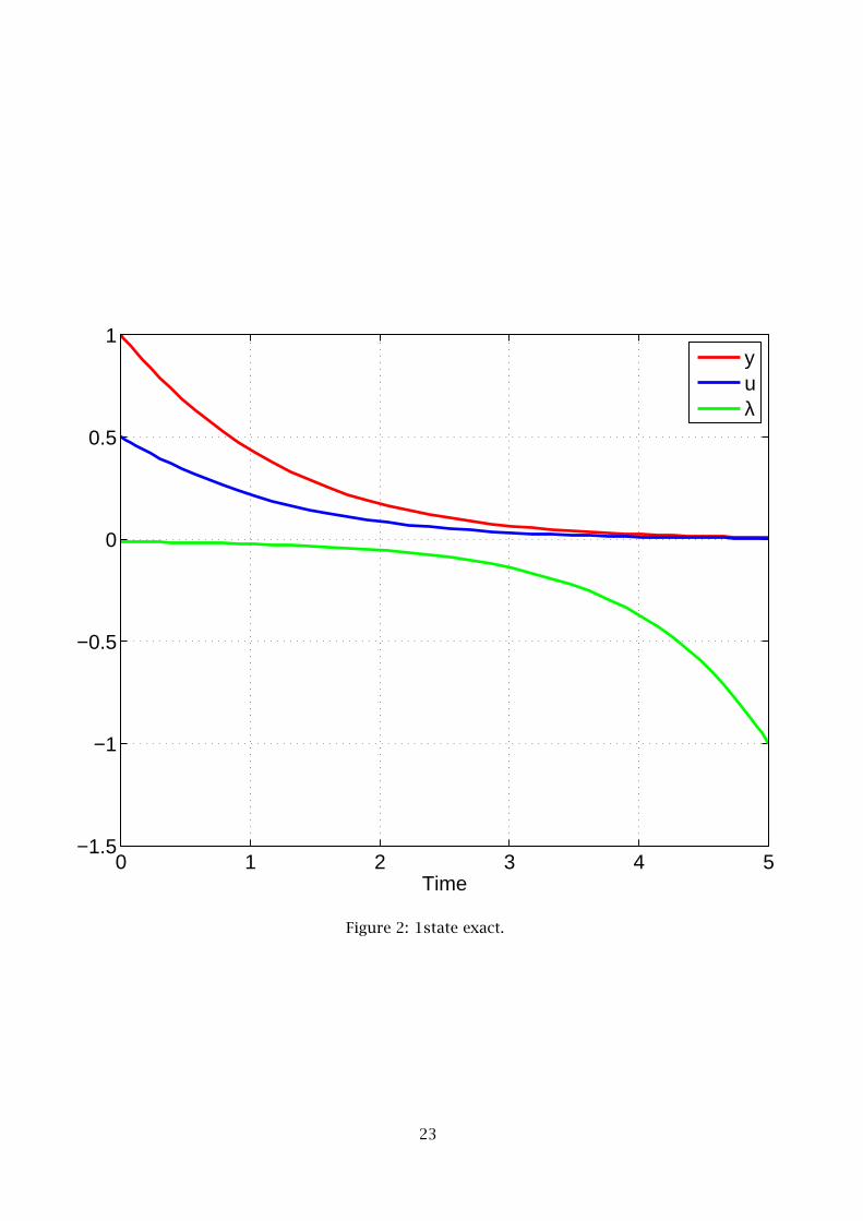
where y(t), is the state, u(t) is the control, and tf = 5 is the final time. The exact solution is

y∗(t) =4

1+ 3et(51)

λ∗(t) = ae(2 ln(1+3et)−t) (52)

u∗(t) = .5y∗(t) (53)

where a =−1

(e−5 + 6+ 9e5)(54)

(55)

λ∗(t) is the costate associated with the optimal solution. The exact solution is depicted in Fig. 2.

This problem is solved using all three pseudospectral techniques mentioned previously. Each method

transcribes the optimal control problem into an NLP that consists of 10 nodes (N = 10). Each NLP is

then solved with SNOPT39 using the default feasibility and optimality tolerances (10−6). In Fig. 3, the

absolute value of the error between the NLP state and the exact solution (|Y(τi)−y∗(τi)|, i = 1, . . . , N)

14

is plotted for each node and all three approaches. Note that the error in initial state is not included

since the SNOPT satisfies state equality bounds (i. e. the initial conditions) to double precision (10−16).

When comparing the state accuracy of the three methods in this example, there is no clear method

that outperforms the other two across the entire interval. In fact, the only noticeable difference in

Fig. 3 is that both the GPM and Radau formulations produce an extremely accurate terminal state. It is

hypothesized that the highly accurate terminal state for the GPM is due to the additional quadrature

constraint in the NLP.

The control error is plotted in Fig. 4. As described in Section 5, each method approximates the con­

trol using a different number of points. The LPM discretizes the control at all N discretization points,

while Radau discretizes the control at the (N­1) Radau points, and the Gauss method discretizes the

control at the (N­2) Gauss points. In the Radau discretization, the initial control is missing. Similarly,

in the Gauss discretization, the control at both the initial and final time are missing. These missing

control values can be found by a variety of techniques. The approach often outlined in the litera­

ture6,19 is to extrapolate the control approximation equations, Eqs. (17), (23) and (29). However, in

practice it is more common to use a simple spline extrapolation.40 Thirdly, a technique involving the

HBVP equations at the boundaries has been developed for the Gauss pseudospectral method.41 Since

these extrapolated controls are not explicit variables in the NLP, one would assume that they would

be less accurate than methods that include the boundary controls in the formulation of the NLP. In

Fig. 4, the boundary control estimate for the Gauss method is indeed the least accurate. Likewise, the

accuracy of the initial control estimate for the Radau method is similar to the GPM value. However, it

is interesting that while the largest error for Gauss and Radau are at the boundaries, the LPM has a

larger error at one of the interior points. The benefit of an accurate initial control is eliminated by a

very inaccurate interior point in the LPM.

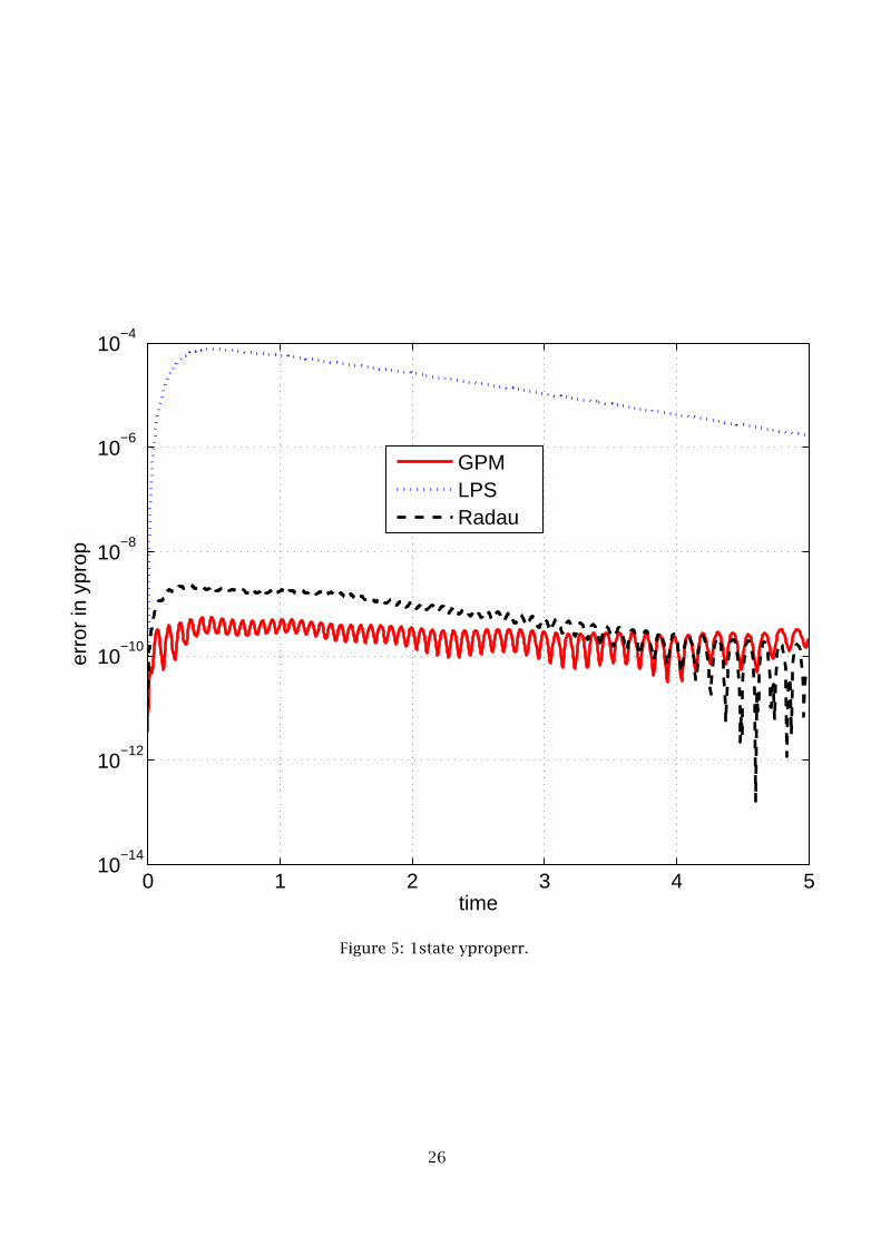
A more appropriate way to determine the effect of the control error is to actually propagate the

state dynamics according to the control estimate from the NLP. In this research, the state dynamics

are propagated using the Matlab function ODE45, where the control approximations are represented

using Eqs. (17), (23), and (29). The resulting propagated state error is shown in Fig. 5. Clearly, the LPM

propagation error is the largest despite the relatively accurate boundary controls.

The largest discrepancy between the methods is seen in the costate comparison of Fig. 6. The LPM

costate approximation is several orders of magnitude worse than the other two methods across all

nodes. This example highlights a common problem26 with the original LPM costate approximation25

where the approximation tends to “wiggle” about the true solution, as shown in Fig. 7. Further­

more, note that the largest error in the LPM costate occurs at the boundaries due to the conflicting

constraints (explained in Section 6.1). The GPM method, which has no constraint conflict, provides

extremely accurate boundary costates, while the RPM method produces an accurate initial costate (no

conflict) but a less accurate final costate (which has a conflict explained in Section 6.2).

In pseudospectral methods, like most direct methods, the solution accuracy can be improved by

increasing the number of nodes used to discretize the problem.11 Furthermore, the rate of conver­

gence to the true optimal solution is extremely important as it can help determine how many nodes

are needed in order to adequately approximate the solution. The convergence rates of the state and

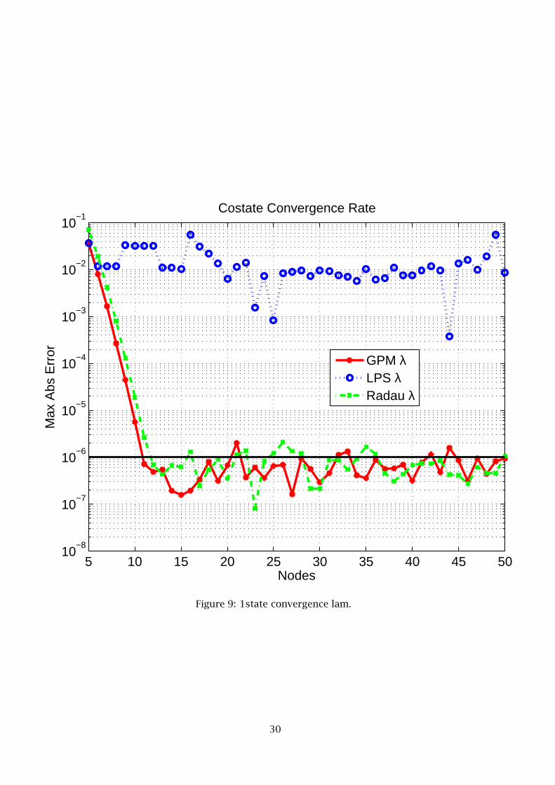
costate are shown in Figs. 8­9, respectively. In these figures, each method was solved repeatedly while

the number of nodes in the problem was increased from 5 to 50. The error shown in these figures is

the maximum absolute error over all the nodes in the problem (||X(τi) − x∗(τi)||∞, ∀τi ∈ [−1,1]).

As seen in Figure 8, the state convergence rate for all three methods is quite similar. The steep

convergence initially seen depicts the “spectral” convergence that is characteristic of pseudospectral

methods.8 Naturally, once the error drops below the tolerances of the NLP, the convergence rate stops

improving. The convergence rate for the costate is shown in Fig. 9. The Gauss and Radau methods

show rapid convergence rates for the costate, which are even faster than the state. Fig. 9 also shows

15

the apparent lack of convergence for the costate using the LPM. It is clear that increasing the number

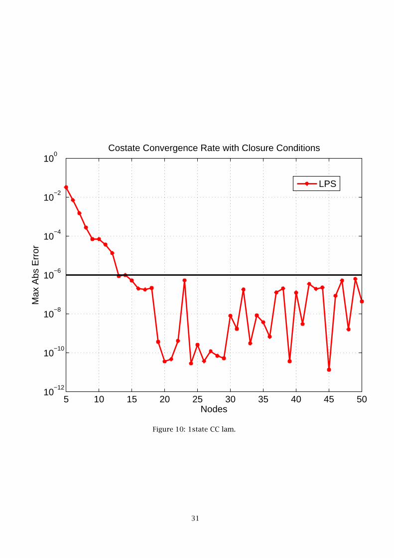
of nodes does not improve the costate error for this example. As mentioned previously, Gong and

Ross have devised a modified covector mapping theorem to improve the costate approximation for

the LPM. This covector mapping theorem includes a set of “closure conditions” that is assumed to

be implemented in a mixed primal­dual feasibility problem where the variables are the state, control,

and costate. The constraints in this primal­dual feasibility problem are the KKT conditions of the

NLP and the additional closure conditions. When this alternate NLP is posed and solved, the resulting

costate convergence in Fig. 10 is indeed much better, although it is still not as rapid as either the

Gauss or Radau methods. As mentioned previously, this increased accuracy comes at a significant

computational burden in post­processing. Due to the large number of extra steps necessary to pro­

duce this result, further computation of LPM costates will involve only the original costate estimation

procedure of Eq. (34), since this is the likely method to be used in practice.

8 Two State Example

As a second example, consider the following two­dimensional optimal control problem. Minimize the

cost functional

J = y2(tf ) (56)

subject to the dynamic constraints

y1(t) = 0.5y1(t)+u(t) (57)

y2(t) = y21 (t)+ 0.5u2(t) (58)

and the boundary conditions,

y1(t0) = 1 y1(tf ) = 0.5 (59)

y2(t0) = 0 (60)

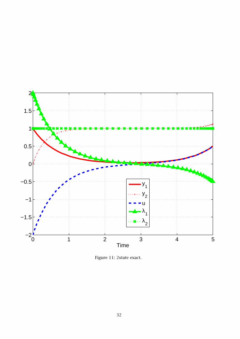
where tf = 5. Note that this problem contains a terminal bound on the first state, y1(tf ). The exact

solution is of the form

y∗1 (t) = a1e1.5t + a2e

−1.5t , (61)

y∗2 (t) = a3(e1.5t)2 − a4(e

−1.5t)2 + c1, (62)

λ∗1 (t) = a5e1.5t + a6e

−1.5t , (63)

λ∗2 (t) = 1, (64)

u∗(t) = −λ∗1 (t) (65)

The exact solution can be seen in Fig. 11. Again, all three methods are compared using 10 nodes.

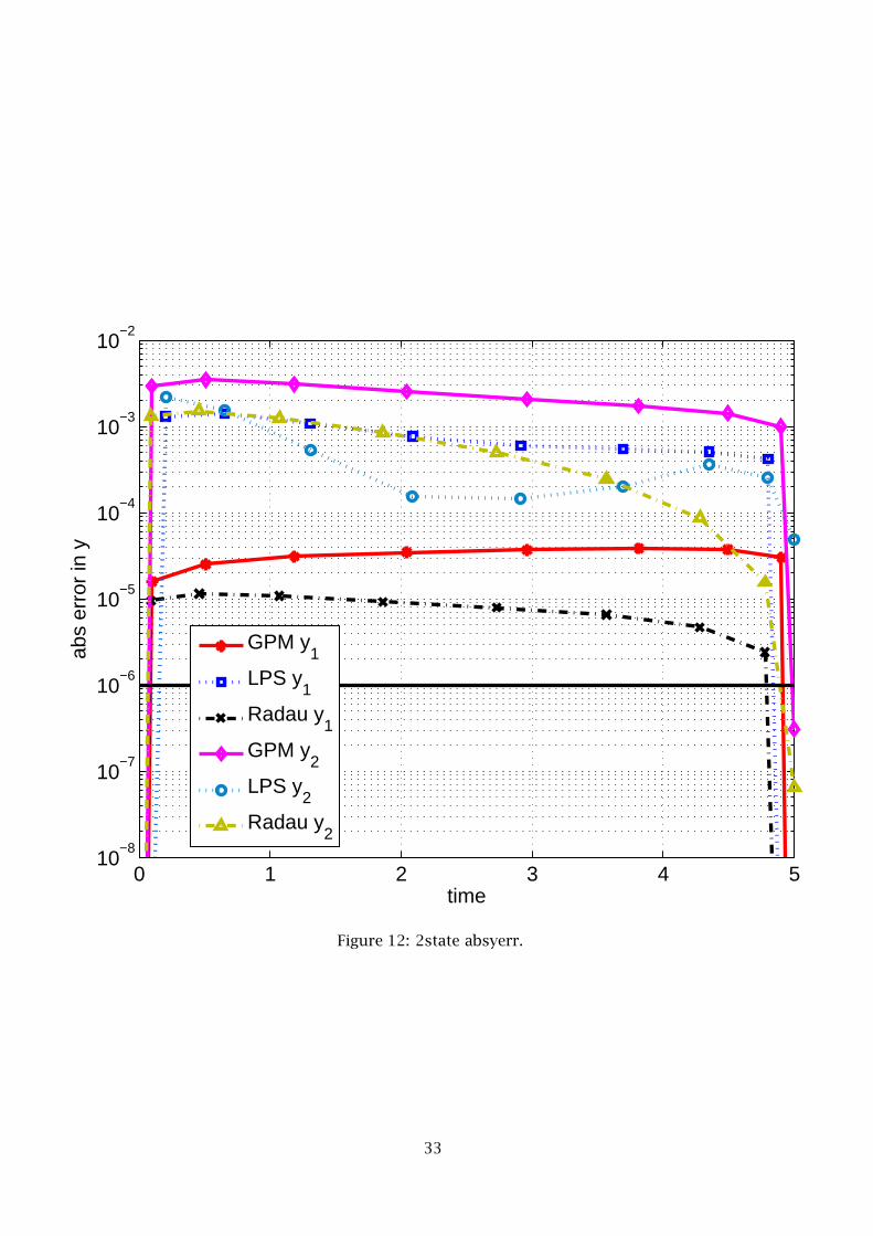
The error plots are formulated in the same manner as the previous example problem. Fig. 12 shows

the state error at each node for all three methods. Recall that the error for the states involving the

boundary conditions is O(10−16), and therefore outside the range of the plot. As in the single­state

example, all three methods are relatively comparable in state accuracy. Moreover, the GPM and Radau

formulations show again show an increase in accuracy for the terminal state.

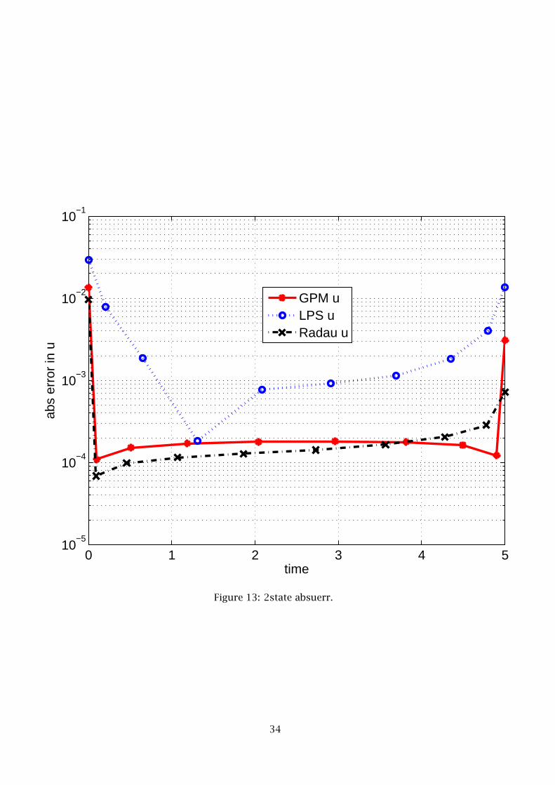
The control error is plotted in Fig. 13. Interestingly, for this problem, the LPM control estimate is

worse than both GPM and RPM, even at the boundaries. The NLP control is used to propagate the state

equations, and their resulting state accuracy is compared in Fig. 14 for both states. In this example,

the RPM produces the most accurate approximation, followed by the GPM, and lastly LPM.

16

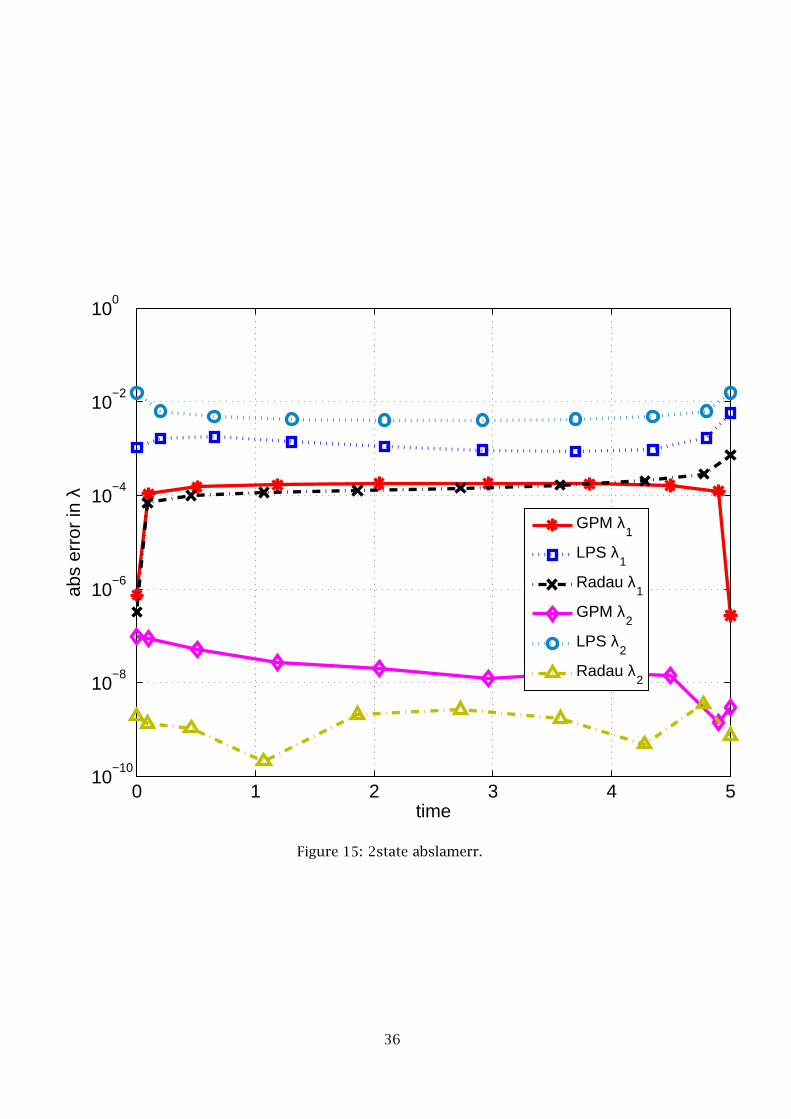
Reconfirming the results in the first example, the largest discrepancy between the methods is

seen in the costate comparison, and specifically with the second costate, shown in Fig. 15. The LPM

method produces the worst costate approximation for both λ1 and λ2. Although it is not shown, this

large error in λ2 is due to the same “wiggle” phenomenon around the true costate as seen in the first

example. The GPM method also provides the most accurate boundary costates, and the Radau method

provides a relatively accurate initial costate, but an inaccurate final costate. In the Radau method, the

final costate is consistently the least accurate costate, suggesting that the conflicting HBVP equations

described in Section 6.2 is degrading the performance of this method.

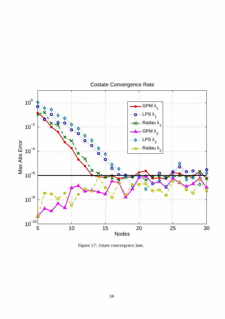
The convergence rates of the state and costate are shown in Figs. 16­17, respectively. Each ap­

proach was solved repeatedly while the number of nodes in the problem was increased from 5 to 30.

The error shown in these figures is computed in the same manner as the previous example. Fig. 16

displays both states, y1 and y2, where there is a noticeable difference between the convergence rate

of y1 and y2 for the GPM and RPM. However, for the LPM approach, both states converge at the same

(slower) rate. The convergence rate of the RPM is the fastest for this example. It is hypothesized

that this slight improvement over the GPM state approximation is due to the one order reduction

in the state approximation for the GPM. Similar results are seen in the costate convergence plot of

Fig. 17. The second costate is constant in this example, and both the GPM and RPM approaches

can approximate this first order polynomial quite well, even using only a few nodes, as expected with

pseudospectral methods. However, the LPM approach displays the wiggle phenomenon and thus has a

much slower convergence rate for λ2. In term of the first costate, the GPM has the fastest convergence

rate.

9 Orbit­Raising Problem

Consider the problem of transferring a spacecraft from an initial circular orbit to the largest possible

circular orbit in a fixed time using a low­thrust engine. This problem is modeled using radius, r(t),

radial velocity, u(t), and tangential velocity, v(t), as the components of the state. The control, φ(t),

is the angle between the thrust vector and the tangential velocity. The optimal control problem is

stated as follows. Minimize the cost functional

J = −r(tf ) (66)

subject to the dynamic constraints

r = u

u =v2

r−µ

r2+

T sinφ

m0 − |m|t

v = −uv

r+

T cosφ

m0 − |m|t

(67)

and the boundary conditions

r(0) = 1, r(tf ) = free

u(0) = 0, u(tf ) = 0,

v(0) =√

µr(0) , v(tf ) =

√

µr(tf )

,(68)

where µ is the gravitational parameter, T is the thrust magnitude, m0 is the initial mass, and m is the

fuel consumption rate. These parameters are given as follows in normalized units:

T = 0.1405, m = 0.0749, m0 = µ = 1, tf = 3.32 (69)

17

This problem does not have an analytic solution, but it has been solved numerically many times38,42

so it’s solution is well known. The results of each method was compared against the solution to

a boundary value problem solution using the Matlab function BVP4C with a tolerance of 10−9. For

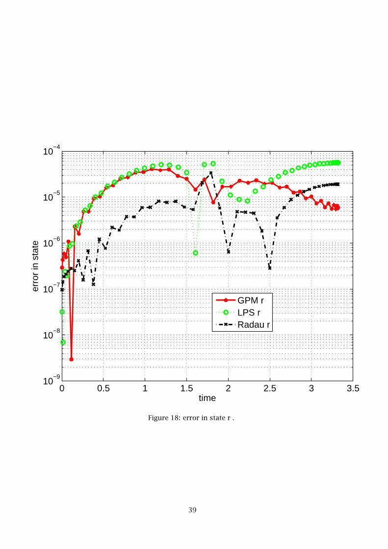
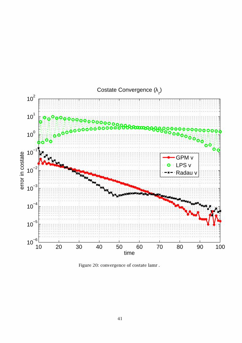
brevity, we present an error analysis for only the first state and costate, r(t) and λr (t). The remaining

state and costate errors look very similar to the one presented. For this problem, the RPM has a

slightly better state accuracy than the other two methods in Fig. 18. Interestingly, for this example,

the RPM also has a slightly better costate approximation than the other two methods as seen in Fig. 19.

As in the previous examples, the LPM costate convergence is significantly worse than the other two

methods.

Based on the results of all three example problems and a detailed analysis of the mathematics

of each method, we can conclude that there may be certain circumstances under which each method

should be chosen. Inaccurate boundary costates in the LPM method are attributed to boundary costs

or constraints in the problem. However, if the original problem has no boundary constraints or

costs, then the conflicting HBVP equations disappear and LPM would be an appropriate method. The

RPM costate inaccuracy only occurs at the terminal time, so problems without terminal constraints

would likely mitigate the errors in the final costate. The GPM has a perfect mapping with the HBVP

equations, and therefore will create accurate costate estimates for problems with both initial and final

constraints.

Lastly, Table 2 presents NLP computation times for all three examples and all three methods.

The results listed correspond to a Pentium 4, 3.2 GHz machine, where the constraint Jacobian was

computed using numerical derivatives. All three methods have very similar computation times, which

is expected since the methods are very similar in terms of their problem density.

10 Conclusions

A comparison has been made between three established pseudospectral methods that have been used

in recent years in the numerical solution of optimal control problems. In particular, the Legendre,

Radau, and Gauss pseudospectral methods have been compared in terms of the accuracy of the state,

control, and costate. Three examples are used in the study to identify the key differences between

the three methods. The results of this study indicate that the accuracy of the Radau and Gauss meth­

ods are very similar in accuracy, while both of these methods significantly outperform the Legendre

method in terms of costate accuracy. Furthermore, it is found that the computational efficiency of the

three methods is quite comparable. Based on these results and a detailed analysis of the mathematics

of each method, a rationale has been constructed to determine when each method should be chosen.

References

1Kirk, D. E. , Optimal Control Theory, Prentice­Hall, Englewood Cliffs, NJ, 1970.

2Pontryagin, L.S., Boltyanskii, V., Gamkrelidze, R., Mischenko, E., The Mathematical Theory of Optimal

Processes. New York: Interscience, 1962.

3Betts, John T., “Survey of Numerical Methods for Trajectory Optimization," Journal of Guidance,

Control, and Dynamics, Vol. 21, No. 2, March­April 1998

4Hull, D. , “Conversion of Optimal Control Problems into Parameter Optimization Problems,” AIAA

Guidance, Navigation, and Control Conference, San Diego, CA, July 29­31, 1996

18

5Vasantharajan, S. , and Biegler, L. T. , “Simultaneous Strategies for Optimization of Differential­

Algebraic Systems with Enforcement of Error Criteria,” Computers and Chemical Engineering, Vol.

14, No. 10, pp.1083­1100, 1990.

6Elnagar, G., Kazemi, M., Razzaghi, M., “The Pseudospectral Legendre Method for Discretizing Opti­

mal Control Problems," IEEE Transactions on Automatic Control, Vol. 40, No. 10, October 1995

7Canuto, C., Hussaini, M.Y., Quarteroni, A., Zang, T.A., Spectral Methods in Fluid Dynamics, Springer­

Verlag, New York, 1988.

8Fornberg, B., A Practical Guide to Pseudospectral Methods, Cambridge University Press, 1998.

9Villadsen, J. , and Michelsen, M. , “Solution of differential equation models by polynomial approxi­

mation,” Prentice Hall, New Jersey, 1978.

10Cuthrell, J. E. , and Biegler, L. T. , “On the Optimization of DIfferential­Algebraic Process Systems,”

AIChE Journal, Vol.33, No.8, pp.1257­1270, Aug. 1987.

11Trefethen, L. N., Spectral Methods in MATLAB, SIAM Press, Philadelphia, 2000.

12Elnagar, G. E. , and Kazemi, M. A. , “Pseudospectral Legendre­based optimal computation of nonlin­

ear constrained variational problems,” Journal of Computational and Applied Mathematics, Vol. 88,

pp.363­375, 1997.

13Fahroo, F. , and Ross, I. M. , “A Spectral Patching Method for Direct Trajectory Optimization,” Journal

of the Astronautical Sciences, Vol. 48, No. 2­3, pp.269­286, Apr­Sept 2000.

14Ross, I. M. , and Fahroo, F. , “A Direct Method for Solving Nonsmooth Optimal Control Problems”,

Proceedings of the 2002 World Congress of the International Federation on Automatic Control, IIAC,

Barcelona, July 2002.

15Rao, A. V. , “Extension of a Pseudospectral Legendre Method to Non­Sequential Multiple­Phase Opti­

mal Control Problems”, AIAA Guidance, Navigation, and Control Conference, AIAA Paper No. 2003­

5634, Austin, TX, Aug. 11­14, 2003.

16Ross, I. M. , and Fahroo, F. , “Pseudospectral Knotting Methods for Solving Optimal Control Prob­

lems,” Journal of Guidance, Control, and Dynamics, Vol. 27, No. 3, 2004.

17Cuthrell, J. E. , and Biegler, L. T. , “Simultaneous Optimization and Solution Methods for Batch

Reactor Control Profiles,” Computers and Chemical Engineering, Vol. 13, No.1/2, pp.49–62, 1989.

18Reddien, G. W. , “Collocation at Gauss Points as a Discretization in Optimal Control,” SIAM Journal

of Control and Optimization, Vol. 17, No. 2, March 1979.

19Kameswaran, S. and Biegler, L. T., “Convergence Rates for Dynamic Optimization Using Radau Col­

location,” SIAM Conference on Optimization, Stockholm, Sweden, 2005.

20Fahroo, F. and Ross, I., “Pseudospectral Methods for Infinite Horizon Nonlinear Optimal Control

Problems,” 2005 AIAA Guidance, Navigation, and Control Conference, AIAA Paper 2005­6076, San

Francisco, CA, August 15–18, 2005.

21Kameswaran, S. and Biegler, L. T., “Convergence Rates for Direct Transcription of Optimal Control

Problems at Radau Points,” Proceedings of the 2006 American Control Conference, Minneapolis,

Minnesota, June 2006.

19

22Vlassenbroeck, J. and Van Doreen, R., “A Chebyshev Technique for Solving Nonlinear Optimal Con­

trol Problems,” IEEE Transactions on Automatic Control, Vol. 33, No. 4, 1988, pp. 333–340.

23Vlassenbroeck, J., “A Chebyshev Polynomial Method for Optimal Control with State Constraints,”

Automatica, Vol. 24, 1988, pp. 499–506.

24Benson, D. A., Huntington, G. T., Thorvaldsen, T. P., and Rao, A. V., Direct Trajectory Optimization

and Costate Estimation via an Orthogonal Collocation Method, Journal of Guidance, Control, and

Dynamics, Vol. 29, No. 6, 2006, pp. 1435–1440.

25Fahroo, F. and Ross, I. M., “Costate Estimation by a Legendre Pseudospectral Method,” Journal of

Guidance, Control, and Dynamics, Vol. 24, No. 2, March­April 2002, pp. 270­277.

26Gong, Q. , Ross, I. , Kang, W. , and Fahroo, F. , “On the Pseudospectral Covector Mapping Theorem

for Nonlinear Optimal Control,” IEEE Conference on Decision and Control, Dec 13­15, 2006.

27Williams, P. , “Jacobi Pseudospectral Method for Solving Optimal Control Problems”, Journal of

Guidance, Vol. 27, No. 2,2003

28Williams, P. , “Hermite­Legendre­Gauss­Lobatto Direct Transcription Methods In Trajectory Opti­

mization,” Advances in the Astronautical Sciences. Vol. 120, Part I, pp. 465­484. 2005

29Williams, P. , “A Comparison of Differentiation and Integration Based Direct Transcription Methods”,

AAS/AIAA Space Flight Mechanics Conference, Copper Mountain, CO, Jan. 23­27, 2005. Paper AAS

05­128.

30Fahroo, F. and Ross, I. M., “Direct Trajectory Optimization by a Chebyshev Pseudospectral Method,”

Journal of Guidance, Control, and Dynamics, Vol. 25, No. 1, January­February 2002, pp. 160–166.

31Gong, Q. , Kang, W. , and Ross, I. , “A Pseudospectral Method for the Optimal Control of Constrained

Feedback Linearizable Systems”, IEEE Transactions on Automatic Control, Vol. 51, No. 7, July 2006.

32Paris, S. W. , Riehl, J. P. , Sjuaw, W. .K. , “Enhanced Procedures for Direct Trajectory Optimization

Using Nonlinear Programming and Implicit Integration,” AIAA/AAS Astrodynamics Specialist Con­

ference and Exhibit, Keystone CO, Aug 2006

33Fahroo, F. , Ross, I. M. , “On Discrete­Time Optimality Conditions for Pseudospectral Methods,”

AIAA/AAS Astrodynamics Specialist Conference and Exhibit, Keystone, CO, Aug 2006.

34Hull, D. G., Optimal Control Theory for Applications, Springer­Verlag, New York, 2003.

35Davis, P., Interpolation & Approximation, Dover Publications, 1975.

36Davis, P., Rabinowitz, P., Methods of Numerical Integration, Academic Press, 1984.

37Williams, P. , “A Gauss­Lobatto Quadrature Method For Solving Optimal Control Problems,” Australia

Mathematical Society, ANZIAM J.47, pp.C101­C115, July, 2006.

38Benson, D., A Gauss Pseudospectral Transcription for Optimal Control, Ph.D. Dissertation, Depart­

ment of Aeronautics and Astronautics, Massachusetts Institute of Technology, November 2004.

39Gill, P.E., Murray, W., and Saunders, M.A., “SNOPT: An SQP Algorithm for Large Scale Constrained

Optimization,” SIAM Journal on Optimization, Vol. 12, No. 4, 2002

20

40Betts, John T., Practical Methods for Optimal Control Using Nonlinear Programming , SIAM. (2001)

41Huntington, G. T., Benson, D. A., and Rao, A. V., “Post­Optimality Evaluation and Analysis of a

Formation Flying Problem via a Gauss Pseudospectral Method,” Proceedings of the 2005 AAS/AIAA

Astrodynamics Specialist Conference, AAS Paper 05­339, Lake Tahoe, California, August 7–11, 2005.

42Bryson, A., Ho, Y., Applied Optimal Control, Blaisdell Publishing Co. (1969)

21

Tra

nscrip

tion a

tG

auss P

oin

ts

OptimalityConditions

OptimalityConditions

Tra

nscrip

tion a

tG

auss P

oin

ts

Continuous-TimeOptimal Control Problem

Continuous HBVP

Discrete HBVP

KKT Conditions

CostateMapping

Indirect

Direct

Discrete NLP

Figure 1: Direct vs Indirect Flow Diagram.

22

0 1 2 3 4 5−1.5

−1

−0.5

0

0.5

1

Time

yuλ

Figure 2: 1state exact.

23

0 1 2 3 4 510

−10

10−9

10−8

10−7

10−6

10−5

10−4

abs

erro

r in

y

time

GPM y

LPS y

Radau y

Figure 3: 1state absyerr.

24

0 1 2 3 4 510

−7

10−6

10−5

10−4

10−3

10−2

10−1

abs

erro

r in

u

time

GPM uLPS uRadau u

Figure 4: 1state absuerr.

25

0 1 2 3 4 510

−14

10−12

10−10

10−8

10−6

10−4

erro

r in

ypr

op

time

GPM LPS Radau

Figure 5: 1state yproperr.

26

0 1 2 3 4 510

−9

10−8

10−7

10−6

10−5

10−4

10−3

10−2

10−1

abs

erro

r in

λ

time

GPM λ

LPS λ

Radau λ

Figure 6: 1state abslamerr.

27

0 1 2 3 4 5−0.04

−0.03

−0.02

−0.01

0

0.01

0.02

0.03

time

cost

ate

erro

r

λ err

Figure 7: 1state lamerr.

28

5 10 15 20 25 30 35 40 45 5010

−10

10−8

10−6

10−4

10−2

100

State Convergence Rate

Nodes

Max

Abs

Err

or

GPM yLPS yRadau y

Figure 8: 1state convergence y.

29

5 10 15 20 25 30 35 40 45 5010

−8

10−7

10−6

10−5

10−4

10−3

10−2

10−1

Costate Convergence Rate

Nodes

Max

Abs

Err

or

GPM λLPS λRadau λ

Figure 9: 1state convergence lam.

30

5 10 15 20 25 30 35 40 45 5010

−12

10−10

10−8

10−6

10−4

10−2

100

Costate Convergence Rate with Closure Conditions

Nodes

Max

Abs

Err

or

LPS

Figure 10: 1state CC lam.

31

0 1 2 3 4 5−2

−1.5

−1

−0.5

0

0.5

1

1.5

2

Time

y1

y2

uλ

1

λ2

Figure 11: 2state exact.

32

0 1 2 3 4 510

−8

10−7

10−6

10−5

10−4

10−3

10−2

abs

erro

r in

y

time

GPM y1

LPS y1

Radau y1

GPM y2

LPS y2

Radau y2

Figure 12: 2state absyerr.

33

0 1 2 3 4 510

−5

10−4

10−3

10−2

10−1

abs

erro

r in

u

time

GPM uLPS uRadau u

Figure 13: 2state absuerr.

34

0 1 2 3 4 510

−10

10−9

10−8

10−7

10−6

10−5

10−4

10−3

10−2

erro

r in

ypr

op

time

GPM y1

GPM y2

LPS y1

LPS y2

Radau y1

Radau y2

Figure 14: 2state yproperr.

35

0 1 2 3 4 510

−10

10−8

10−6

10−4

10−2

100

abs

erro

r in

λ

time

GPM λ1

LPS λ1

Radau λ1

GPM λ2

LPS λ2

Radau λ2

Figure 15: 2state abslamerr.

36

5 10 15 20 25 3010

−7

10−6

10−5

10−4

10−3

10−2

10−1

100

State Convergence Rate

Nodes

Max

Abs

Err

or

GPM y

1

LPS y1

Radau y1

GPM y2

LPS y2

Radau y2

Figure 16: 2state convergence y.

37

5 10 15 20 25 3010

−10

10−8

10−6

10−4

10−2

100

Costate Convergence Rate

Nodes

Max

Abs

Err

or

GPM λ1

LPS λ1

Radau λ1

GPM λ2

LPS λ2

Radau λ2

Figure 17: 2state convergence lam.

38

0 0.5 1 1.5 2 2.5 3 3.510

−9

10−8

10−7

10−6

10−5

10−4

erro

r in

sta

te

time

GPM rLPS rRadau r

Figure 18: error in state r .

39

0 0.5 1 1.5 2 2.5 3 3.510

−6

10−5

10−4

10−3

10−2

10−1

100

101

erro

r in

cos

tate

time

GPM λr

LPS λr

Radau λr

Figure 19: error in costate lamr .

40

10 20 30 40 50 60 70 80 90 10010

−6

10−5

10−4

10−3

10−2

10−1

100

101

102

erro

r in

cos

tate

time

Costate Convergence (λr)

GPM vLPS vRadau v

Figure 20: convergence of costate lamr .

41

Table 1: Definitions of Lagrange interpolation polynomials used in this work

# of Basis Polynomials Application Symbol Index

N LPM (x,u,λ) Li(τ) i = 1, . . . , N

N RPM (x) Li(τ) i = 0, . . . , N − 1

N­1 RPM (u,λ) Li(τ) i = 1, . . . , N − 1

N­1 GPM (x,λ) Li(τ) i = 0, . . . , N − 2

N­2 GPM (u) Li(τ) i = 1, . . . , N − 2

42

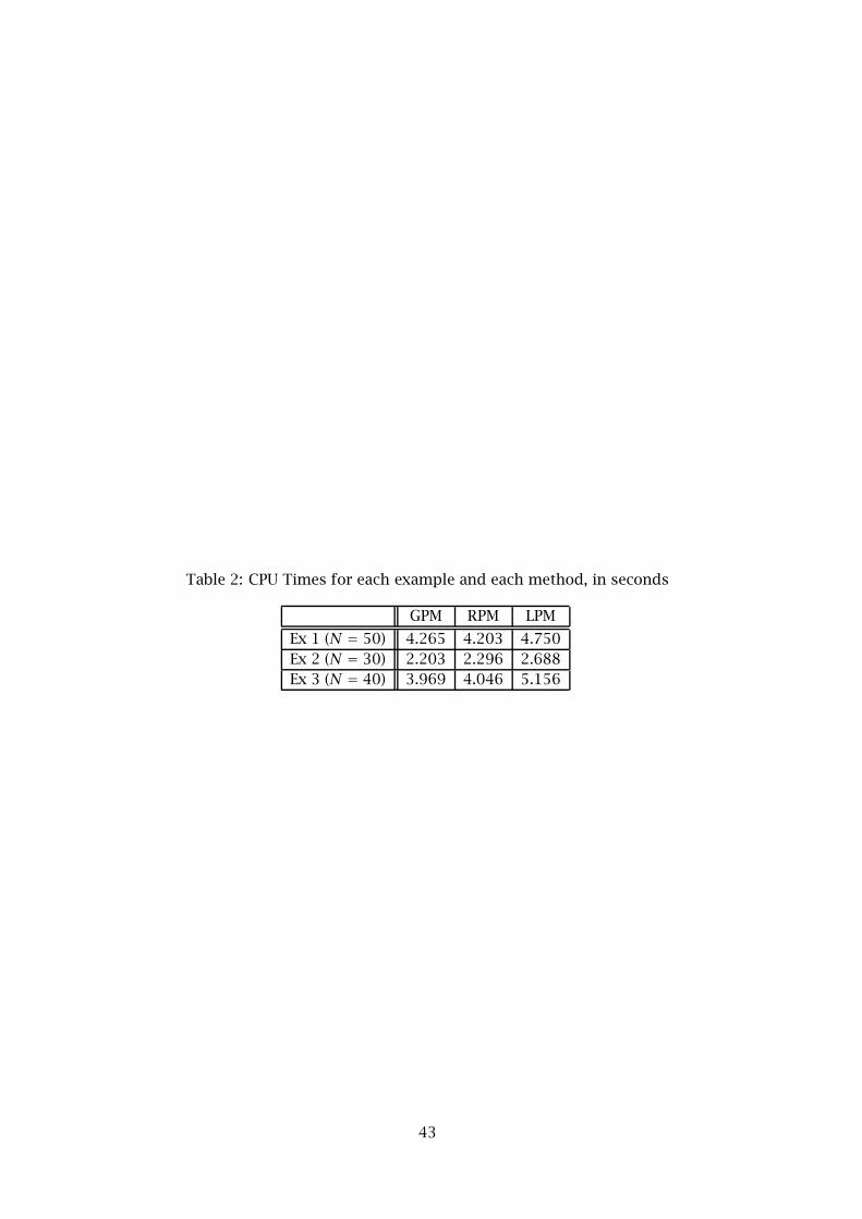
Table 2: CPU Times for each example and each method, in seconds

GPM RPM LPM

Ex 1 (N = 50) 4.265 4.203 4.750

Ex 2 (N = 30) 2.203 2.296 2.688

Ex 3 (N = 40) 3.969 4.046 5.156

43