A Comparative Study of Real Options Valuation Methods:

Economics-Based Approach vs. Engineering-Based Approach

by

Shuichi Masunaga

Bachelor of Laws

University of Tokyo, 1999

Submitted to the Department of Urban Studies and Planning

in Partial Fulfillment of the Requirements for the Degree of

Master of Science in Real Estate Development

at the

Massachusetts Institute of Technology

September, 2007

© 2007 Shuichi Masunaga

All rights reserved

The author hereby grants to MIT permission to reproduce and to distribute publicly paper and electronic

copies of this thesis document in whole or in part in any medium now known or hereafter created.

Signature of Author______________________________________________________

Department of Urban Studies and Planning July 27, 2007

Certified by_____________________________________________________________

David Geltner Professor of Real Estate Finance,

Department of Urban Studies and Planning Thesis Advisor

Accepted by_____________________________________________________________

David Geltner Chairman, Interdepartmental Degree Program

in Real Estate Development

A Comparative Study of Real Options Valuation Methods:

Economics-Based Approach vs. Engineering-Based Approach

by

Shuichi Masunaga

Submitted to the Department of Urban Studies and Planning on July 27, 2007

in Partial Fulfillment of the Requirements for the Degree of Master of Science in Real Estate Development

Abstract

It has been expected that the option valuation theory will play a much more

significant role in the real estate analysis. However, potentially because of the need for

understanding the advanced financial theories, the real options analysis has not been fully

used in the real world. In order to attack this problem, it is highly desired to create a more

practical and easily understandable calculation model for valuing flexibility.

With the increasing computational power of today, an interesting approach to

valuing flexibility arises from the field of engineering systems. This approach does not

require the understanding of advanced financial theories, and aims to assess the value of

flexibility built into the project design. Although the perspective of this approach may be

slightly different from that of traditional real options valuation approach, this approach

might be an alternative method as a simpler model for valuing flexibility.

The comparative study of the economics-based approach and the engineering-

based approach revealed that the latter approach has one critical problem in estimating

the value of flexibility; the usage of a single risk-adjusted discount rate leads to either

underestimation or overestimation of the real options value. Based on the results of a case

study, this thesis proposes to use the engineering-based approach together with the

economics-based approach. With its ability of comprehensive analysis and graphic

presentation, the engineering-based approach has a great probability to make it easier for

average practitioners to intuitively understand the value of flexibility.

Thesis Supervisor: David Geltner

Title: Professor of Real Estate Finance,

Department of Urban Studies and Planning

2

Acknowledgments

I would like to thank gratefully Professor David Geltner, my thesis supervisor at MIT

Center for Real Estate, for providing valuable guidance and advice on this thesis. I would

also like to thank him for inspiring us with plenty of cutting-edge knowledge throughout

the academic year at MIT/CRE.

I am grateful to Professor Richard de Neufville and Michel-Alexandre Cardin for their

generous advice on my research. This thesis started from the inspiration they gave to me

in the Advanced Topics in R.E. Finance course. I hope this thesis will provide a small

contribution to their further work.

I am thankful to my classmates Katie and Baabak, who have explored this interesting,

and rather troublesome topic with me, and also I am thankful to all MSRED classmates.

It was a really great experience to study with you all at MIT.

I would also like to thank my friends who have supported me throughout the year;

especially my thanks go to Ai, Yoko, Kohichi, Mio, Natsuko, Kohei, Kazuko, and Reiko.

Finally, I am grateful to my father and mother, and all the people who encouraged me to

pursue the Master’s degree in the United States. This experience has been a lot more

exciting and meaningful than I had expected.

3

Table of Contents

Chapter 1 Introduction.................................................................................................. 8

1.1 Background ............................................................................................................. 9

1.2 Objectives................................................................................................................. 9

Chapter 2 Overview of Real Options Theory ............................................................ 11

2.1 Types of real options ............................................................................................. 11

2.2 Application to real estate development ............................................................... 13

2.3 Solution methods for valuing real options .......................................................... 13

2.3.1 Black-Scholes equation.................................................................................. 15

2.3.2 Binominal option valuation model ............................................................... 16

2.3.3 Monte Carlo simulation method................................................................... 16

2.4 Choice of option calculation methods ................................................................. 17

Chapter 3 Methodology ............................................................................................... 19

3.1 Economics-based approach.................................................................................. 19

3.1.1 Binominal option valuation method ............................................................. 19

3.1.2 Samuelson-McKean formula ........................................................................ 24

3.1.3 Time to build .................................................................................................. 25

3.2 Engineering-based approach ............................................................................... 27

3.2.1 Step 1: Create the most likely initial cash flow pro forma ......................... 28

3.2.2 Step 2: Incorporate uncertain variable(s) into the initial model ............... 29

3.2.3 Step 3: Determine the main sources of flexibility and incorporate into the

model .............................................................................................................. 32

3.2.4 Step 4: Search for the combination of decision rules to maximize value.. 33

4

3.2.5 Scenario categorization and catalog of operating plans ............................. 34

3.3 Common issues in both models ............................................................................ 36

3.3.1 Risk-neutral probability approach vs. “real” probability approach ........ 36

3.3.2 Compound options ......................................................................................... 38

3.3.3 Choice of uncertain variable(s)..................................................................... 39

3.3.4 Movement of uncertain variable(s) .............................................................. 40

Chapter 4 Case Study .................................................................................................. 43

4.1 Case statement....................................................................................................... 43

4.2 Economics-based approach.................................................................................. 46

4.3 Engineering-based approach ............................................................................... 51

4.3.1 Experiment 1 .................................................................................................. 51

4.3.2 Experiment 2 .................................................................................................. 64

4.3 Findings of case study ........................................................................................... 70

Chapter 5 Conclusion .................................................................................................. 72

5

List of Figures

Figure 3.1: Example of binominal option valuation trees......................................... 21 Figure 3.2: Example of the movement of uncertain variable.................................... 31 Figure 3.3: Example of histogram distribution of NPV outcomes ........................... 31 Figure 3.4: Example of Value at Risk and Gain (VARG) curve .............................. 33 Figure 3.5: Four-quadrant real estate market model................................................. 40 Figure 3.6: Example of histogram distribution of future values of uncertain variable

........................................................................................................................... 42 Figure 4.1: Expected built property value and expected construction cost of the RHP

Phase I in static case ......................................................................................... 52 Figure 4.2: Expected built property value and expected construction cost of the RHP

Phase II in static case ........................................................................................ 52 Figure 4.3: Expected abandonment value in static case ........................................... 53 Figure 4.4: Static case pro forma summary (columns are shown semi-annually to

conserve space) ................................................................................................. 54 Figure 4.5: Histogram distribution of the RHP Phase II built property value at month

84 based on 2000 Monte Carlo simulations...................................................... 55 Figure 4.6: Example of one RHP Phase I property value fluctuation from 2000

Monte Carlo simulations................................................................................... 56 Figure 4.7: Inflexible case pro forma summary based on the example in Figure 4.6

(columns are shown semi-annually to conserve space) .................................... 57 Figure 4.8: Histogram distribution of the project NPV in the inflexible case based on

2000 Monte Carlo simulations.......................................................................... 57 Figure 4.9: Histogram distribution of NPV in the flexible case based on 2000 Monte

Carlo simulations .............................................................................................. 60 Figure 4.10: VARG curve based on 2000 Monte Carlo simulations........................ 61 Figure 4.11: Timing of the RHP Phase II option exercise based on trial 2 in Table

4.9 (total 1119 times out of 2000 Monte Carlo simulations)............................ 62 Figure 4.12: Static case pro forma summary (columns are shown semi-annually to

conserve space) ................................................................................................. 65 Figure 4.13: Histogram distribution of the project NPV in the inflexible case based

on 2000 Monte Carlo simulations..................................................................... 66 Figure 4.14: Timing of the RHP project abandonment based on trial 6 in Table 4.12

(total 684 times out of 2000 Monte Carlo simulations).................................... 68 Figure 4.15: Static case NPV, ENPV in flexible case based on trial 2 in Table 4.12,

ENPV in flexible case based on trial 4 in Table 4.12. ...................................... 69

6

List of Tables

Table 4.1: Assumptions of Roth Harbor case ........................................................... 44 Table 4.2: Rentleg Gardens project land value tree (only the first 12 months are

shown to conserve space.)................................................................................. 47 Table 4.3: Present value of 24 months delayed receipt of the RHP Phase II option

value (only the first 12 months are shown to conserve space.) ........................ 48 Table 4.4: Option value of the RHP Phase I (only the first 12 months are shown to

conserve space.) ................................................................................................ 49 Table 4.5: RHP Phase I option optimal decision tree (only the first 12 months are

shown to conserve space.)................................................................................. 49 Table 4.6: The RHP option OCC tree (only the first 12 months are shown to

conserve space.) ................................................................................................ 50 Table 4.7: Comparison of expected value and total volatility of the RHP Phase II

property values at month 84.............................................................................. 55 Table 4.8: Sources of flexibility and decision rules.................................................. 58 Table 4.9: Results of trials to find the best combination of decision rules............... 59 Table 4.10: Comparison of NPV outcomes between the inflexible case and the

flexible case ...................................................................................................... 60 Table 4.11: Number of exercise of the RHP Phase I option, the RHP Phase II option,

and the abandonment option (based on trial 2 in Table 4.9)............................. 62 Table 4.12: Result of trials to find the best combination of decision rules .............. 68 Table 4.13: Number of exercise of the RHP Phase I option, the RHP Phase II option,

and the abandonment option (based on trial 6 in Table 4.12)........................... 68 Table 5.1: Merits and demerits of the economics-based approach and the

engineering-based approach.............................................................................. 73

7

Chapter 1 Introduction

In recent years, many academic studies have been done in search of ways in

which real estate can be rigorously analyzed by applying the option valuation theory

(OVT). It is expected that the real options approach will play much more significant roles

in the real estate industry in the near future. However, when compared with the

Discounted Cash Flow (DCF) approach, which is more traditional and more commonly

used in the real world, the real options approach requires a highly sophisticated

understanding of the underlying financial theory, as well as time and manpower for

analyses. This complexity of the real options approach is one of the main reasons that

prevent this relatively new approach from becoming the mainstream method of valuing

real estate.

In order to clear up this problem, several researchers have been trying to create

practical models for valuing flexibility embedded in real estate, based on easier and more

intuitive procedures.1 An example of these relatively simple models is one which

conducts simulations analyses with Excel® software, which is commonly used in the real

business world. With the increasing computational power of the software, we might be

able to apply the theory of real options to the real world in an easier way, and make real

estate investment decisions more comprehensive. In this thesis, I call this simpler method

the “engineering-based” approach.

In the above contexts, this thesis will aim to compare the engineering-based real

options model with the more theoretical, “economics-based” real options model, which is

represented by the binominal option valuation method in this thesis. If this thesis

1 See, for example, de Neufville, Scholtes, & Wang (2006)

8

successfully verifies that both models can work in exactly the same way, it would be

much better to use the engineering-based approach rather than the economics-based

approach, since the latter requires unfamiliar techniques for decision-makers. If there is

any difference found between the two models, this thesis will clarify the reasons behind it

and try to give suggestions for further sophistication of the engineering-based approach.

1.1 Background

This thesis has been inspired by the research done by Professor Richard de

Neufville and his students at Massachusetts Institute of Technology. Many aspects of the

engineering-based real options model are derived from their studies.

The economics-based real options model I will use for comparison is largely

based on the method presented by Geltner, Miller, Clayton, and Eichholtz (2007). In

Chapter 4 of this thesis, I will also use the case study introduced in this book.

I start by reviewing some related issues addressed in the past studies of the real

options theory in the next chapter, then describe the methodology in Chapter 3, and apply

the two different real options valuation models to a case study in Chapter 4.

1.2 Objectives

The primary objectives of this thesis are as follows:

Create equivalent conditions to compare the engineering-based model with the

economics-based model.

Examine how closely two different real options models can value the flexibility in

real estate development through a case study.

9

Provide suggestions for further improvement of the engineering-based approach.

10

Chapter 2 Overview of Real Options Theory

The term “real options” was first used by Myers (1984) in the context of strategic

corporate planning. More recently, this notion has been broadened to capture various

types of decision making under uncertainty. The basic concept of this notion is that

wherever there is an option, there is a chance to benefit from the upside, while avoiding

downside risk at the same time.

As opposed to traditional financial options, real options basically refer to the

options whose underlying assets are real assets. Especially in the case of real estate, a

typical application of real options theory is the land development option, which can be

seen as a call option. Following the definition by Geltner et al. (2007), the land

development option can give the land owner “the right without obligation to develop (or

redevelop) the property upon payment of construction cost.” This thesis is focused on this

call option model of the land value.

2.1 Types of real options

As many studies have shown (Dixit and Pindyck, 1994; Trigeorgis, 1996; Amram

and Kulatilaka, 1999), many types of decisions could be made by using real options

theory. The main examples of real options are as follows.

Waiting options

When any key factor in the business is uncertain (e.g., rent may be increasing or

decreasing in the case of real estate), we may be able to acquire higher returns by waiting

for a certain period of time than we could acquire by acting immediately.

11

Growth options (Phasing options)

When the project is phased into more than two steps, the initial investment provides the

firm with growth options to be acquired by the second or later investment, given that the

first investment turns out to be successful. In other words, by considering the value of

growth options, the firm may be able to go ahead with the first project even if that project

itself is expected to have a negative return.

Flexibility options (Switching options)

This option refers to the flexibility built into the initial project design. By incorporating

flexibility to react to the uncertainty in the future, the project can have higher value than

the value based on the traditional DCF analysis. In the case of real estate, what is called

“conversion” is an example of switching options (e.g., the option to switch the use from

hotels to condominiums).

Exit options (Abandonment options)

Even when there is a certain amount of risk to continue the project in the future, it could

be possible to initiate the project, taking into consideration the value of the option to exit

from the project when the risk becomes obvious (in the case of real estate, there is an

abandonment option for the land owner of vacant land, which is selling the land without a

building on it).

Learning options

When the project can be developed in a phased manner, the firm can test the suitability of

the projects by developing the initial phase with low costs. Then, based on the result, the

firm can modify (or abandon) the following phase of development in order to maximize

the total project value.

12

2.2 Application to real estate development

It should be noted that the types of real options mentioned above are closely

related to each other, and more often than not, real estate development projects

incorporate more than two of the above real options at the same time. For example,

suppose we are to develop a large-scale, mixed-use real estate project in a multi-phased

manner, and we can modify the development timing as well as the use of each phase

during the development process, or even abandon one or more development phases; the

project can include all of the above real options.

In this thesis, I will focus my discussion on the value of real options in the process

of real estate development. In other words, I regard a developable piece of land as an

American call option, the exercise of which is to begin the construction at any given time,

and the exercise price of which is the construction cost at that time.

2.3 Solution methods for valuing real options

In this section, I will review the types of solution methods for valuing real options,

which are the main focus of this thesis. There are three major solution methods as follows.

Partial differential equation approach

This approach is based on mathematical techniques. As represented by the Black-Scholes

equation, this approach calculates option values by equating the change in option values

with the change in the tracking portfolio values. As discussed later in this thesis, the

Black-Scholes equation and the Samuelson-McKean formula are widely acknowledged

models of this approach.

13

Dynamic programming approach

This approach extends the possible values of the underlying asset through the life of the

option. Then, this approach searches for the optimal strategy at the last period, given the

decision made at the previous period, and discounts the value of the optimal strategy to

time zero in a backward recursive manner. The dynamic programming approach is very

useful and helpful in that it can visually show the movement of the real property as well

as the real option values, and this characteristic makes it easier for the user to understand

the real options intuitively. Also, this approach can deal with more complicated real

options, compared to the partial differential approach.

Simulation approach

The simulation approach extends the value of the underlying asset based on thousands of

possible scenarios from the present to the option expiration time. The most commonly

used simulation approach is the Monte Carlo simulation method. The simulation

approach can also deal with complicated real options, and more importantly, it can solve

the “path dependent” options, which is discussed in detail later.2

Each of these solution methods has many calculation models. I will discuss three

models that represent each of the solution methods above: the Black-Scholes equation,

the binominal option valuation model, and the Monte Carlo simulation method.

2 It should be noted that the simulation approach is often said not to be well suited for American options (Amram and Kulatilaka, 1999; Trigeorgis, 1999; Mun, 2006). This difficulty will be examined later in the case study (Chapter 4).

14

2.3.1 Black-Scholes equation

The most fundamental and acknowledged European call option valuation model is

the Black-Scholes equation, which was developed by Fischer Black, Robert Merton, and

Myron Scholes in the early 1970s. This model is one of many applications of the partial

differential approach. The model was a breakthrough in that it uses the approach known

as the dynamic tracking approach under the no-arbitrage arguments.

Although the Black-Scholes equation apparently has a significant power not only

in the field of financial options but also in the field of real options, this relatively simple

solution cannot always give us the answer of option values. For example, in the case of

real estate development, the land development is usually regarded as a perpetual option

(i.e. the right to develop never expires). However, since the Black-Scholes equation

requires one fixed decision date (European options), it is impossible to give solutions to

more complicated real options such as the one that has a perpetual life and allows

exercise of option at any time (American options). Also, this equation cannot be used for

the options with dividends payment and compound options, which will be discussed in

Chapter 3.

Despite its strengths such as the quickness of the calculation, this model also has

the weakness that it is difficult to see what is really happening behind the model.

Considering the objective of this thesis to examine practical models that can be easily

applied to valuing flexibility in the real world, I do not use the Black-Scholes equation in

this thesis.

15

2.3.2 Binominal option valuation model

Recognizing the strengths and weaknesses of the Black-Scholes equation, many

researchers have tried to create other practical tools and models for valuing more

complex real options such as American options. Among these, the binominal option

valuation model originally developed by Cox, Ross, and Rubinstein (1979) has gained

considerable attention as an example of the dynamic programming approach.3 The

binominal option valuation model has several advantages over other real options models.

In addition to the strength mentioned about the dynamic programming approach in

general, the binominal option valuation model can illustrate the intermediate decision-

making processes between now and the option expiration time, which enables us to

understand intuitively how we should decide at each point in time.

The binominal option valuation model is usually based on the risk-neutral

argument, on which the Black-Scholes equation is also based. Due to this, the model

doesn’t require risk-adjusted discount rates, the need for which sometimes causes

problems in valuing real options.

2.3.3 Monte Carlo simulation method

Another major approach to complex real options valuation is the simulation

approach. This approach calculates the options value by randomly simulating thousands

of possible future scenarios for uncertain variables. The most commonly used simulation

model is the well-known Monte Carlo simulation method, which I will use in the

engineering-based approach in this thesis. One of the strong points of the simulation

3 The typical procedure of the binominal option valuation model will be discussed in detail later in Chapter 3.

16

model is that it enables us to deal with “path dependent” real options. In the case of real

estate development, for example, if the criterion for initiating construction is that the

expected built property value exceeds the construction cost for three consecutive months,

it is clearly possible to determine the point of initiating construction by creating the

simulation model monthly.

In general, the Monte Carlo simulation method would give the same result as the

rigorous economics-based option valuation models such as the Black-Scholes equation

and the binominal option valuation model, if it is based on the risk-neutral dynamics.

However, introducing the risk-neutral dynamics into the Monte Carlo simulation method

reduces the simplicity and the transparency of the model. Considering again the objective

of this thesis, I will try not to use the risk-neutral dynamics in the engineering-based

approach in this thesis.4

2.4 Choice of option calculation methods

In theory, all of the option calculation methods above should give the same result,

as long as the inputs and the application of the financial theories are consistently

structured. Therefore, we should only have to choose the easiest and most familiar model

for any particular real-world case. In reality, however, setting inputs and financial

theories exactly the same may not always be an easy job. An example of typical

differences among these models is that the binominal option valuation model requires

backward calculation, while the simulation method doesn’t necessarily require it. This

4 The difference between the risk-neutral probability approach and the “real” probability approach will be discussed later in Chapter 3.

17

kind of difference in the structure could be a barrier to adopting the same theories in

different calculation methods.

In the following two chapters, I discuss how to input equivalent assumptions in

the economics-based valuation model and the engineering-based valuation model. The

economics-based model refers to the binominal option valuation model described above.

The engineering-based model is based on the Monte Carlo simulation method, but in the

sense that it requires less understanding of real options theory, the engineering-based

model I use is a little different from the “simulation-based” real option model.

In essence, by the term “economics-based” model, we refer to a model that is

consistent with equilibrium within and between three well-functioning markets: the

market for land (i.e., development rights), the market for built property (i.e., the property

market for stabilized operating buildings, the development option “underlying assets”),

and the market for contractual future cash flows (e.g., the bond market, as construction

cost cash flows are contractual). By the term “engineering-based” model, we refer to a

decision analysis type simulation model that is willing to sacrifice some of the above-

noted economic rigor to make the model more transparent and easy to use by real-world

decision-makers.

I discuss the methodology of the economics-based approach and the engineering-

based approach respectively in the next chapter, and then compare the procedure and the

results based on a case study in Chapter 4.

18

Chapter 3 Methodology

In this chapter, I examine two different real options valuation methods. The

economics-based one examined first is the binominal option valuation method, which

will hereafter simply be called the “economics-based” approach. The methodology I will

discuss is mostly based on the one presented by Geltner et al. (2007). The “engineering-

based” methodology I examine subsequently is based on the approach developed by de

Neufville, Scholtes, and Wang (2006) and Cardin (2007), which calculates the value of

flexibility using Monte Carlo simulations in Excel® spreadsheets.

This chapter explores the detailed process of the two methods of option valuation.

In terms of the application of the real options theory, I regard a developable piece of land

as an American call option in the process of real estate development.

3.1 Economics-based approach

3.1.1 Binominal option valuation method

This well-known option valuation method evaluates real options by creating

binominal trees, each node of which represents the actual “up” or “down” of values of the

underlying asset over time. An example of the binominal trees is illustrated in Figure 3.1.

The method introduced here is mostly based on the binominal option valuation method

previously discussed in Chapter 2, with the assumption of the “real” probability

approach.5

The inputs required in the calculation and the variables are as follows:

5 See Arnold and Crack (2003).

19

<Inputs and variables>

Vi,j: Value of the underlying asset at period j, with i representing the total number of

down outcomes out of j periods

Kj: Construction cost at period j, corresponding to V at the same period6

Ci,j: Value of the option (land price) at period j, with i representing the total number of

down outcomes (corresponding to the movement of V) out of j periods

PVt[n]: Present value of n as of period t

Et[n]: Expected value of n as of period t

rv: Expected annual total return on investment in the underlying asset7

yv: Annual net rental income cash payout (yield) as a fraction of current building value

gv: Expected annual growth rate in the underlying asset

* gv+1 = (1+rv) / (1+yv)

p: Probability of the up outcome in each period

* Probability of the down outcome in each period: 1-p

σv: Expected annual volatility of returns on individual underlying asset

rf: Risk-free rate of interest

gk: Expected annual growth rate in the construction cost8

yk: Construction cost yield

* gk+1 = (1+rf) / (1+yk)

6 Here I am assuming instantaneous construction for simplicity. The realistic assumption of “time to build” will be discussed later in this chapter. 7 In this thesis, I assume a constant expected return (rv) as well as a constant volatility (σv) through the life of the option. In more complex cases, it is possible to assume different return expectations at each time. 8 I assume a constant construction cost growth, and also that no matter how the value of built property moves (up or down), construction costs are the same within each period.

20

(expire)period 0 1 2 3 4Value of underlying asset tree (V, ex-dividend)

V0,4

V0,3

probability:p V0,2 V1,4

V0,1 V1,3

V0 V1,2 V2,4

V1,1 V2,3

probability:1-p V2,2 V3,4

V3,3

V4,4

Construction cost tree (K)K4

K3

K2 K4

K1 K3

K0 K2 K4

K1 K3

K2 K4

same value K3

K4

Option value tree (C)C0,4

C0,3

C0,2 C1,4

C0,1 C1,3

C0 C1,2 C2,4

C1,1 C2,3

Option value C2,2 C3,4

C3,3

C4,4

At final period(expiration):

Ci,4 = MAX (Vi,4-K4, 0)

Backward calculationusing certainty-equivalence formula

Figure 3.1: Example of binominal option valuation trees

Figure 3.1 illustrates a conceptual example of the binominal trees. For simplicity, I

assume only four periods (years) until the option’s expiration. First, I develop the tree of

underlying asset values. Supposing that we can observe the current value of the

underlying asset, V0, the values of the underlying asset at one year from now are

calculated as follows:

21

(up case) V0,1 = V0 * (1+σv) / (1+yv)

(down case) V1,1 = V0 / (1+σv) / (1+yv)

In general, this can be set at any one step in the tree as follows:

(up case) Vi,j+1 = Vi,j * (1+σv) / (1+yv) (1)

(down case) Vi+1,j+1 = Vi,j / (1+σv) / (1+yv) (2)

The probability of the up movement is as follows9:

)1/(11)1/(11

vv

vvrpσσσ+−++−+

= (3)

Then, the tree for the construction cost is made in a similar way. In the case of

construction cost, however, there is no need to distinguish up and down cases, or the

probability of movements, because I do not assume volatility in the construction cost.

Therefore, I simply increase the construction cost at each step in the tree by the expected

growth rate.

Kj+1 = Kj * (1+gk)

Next, I calculate the options value starting from the terminal period (year 4 in this case).

Supposing that we do not develop the land and wait until year 4, then our decision is

either (1) start construction at year 4, or (2) abandon the project. Therefore, the option

values at the terminal period should equal the maximum of either immediate exercise or

abandonment, which are calculated as follows:

Ci,4 = MAX[Vi,4 – K4, 0]

In general, let T donate the terminal period:

Ci,T = MAX[Vi,T – KT, 0] (4)

9 Since I assume constant levels for rv and σv, p is also assumed to be constant.

22

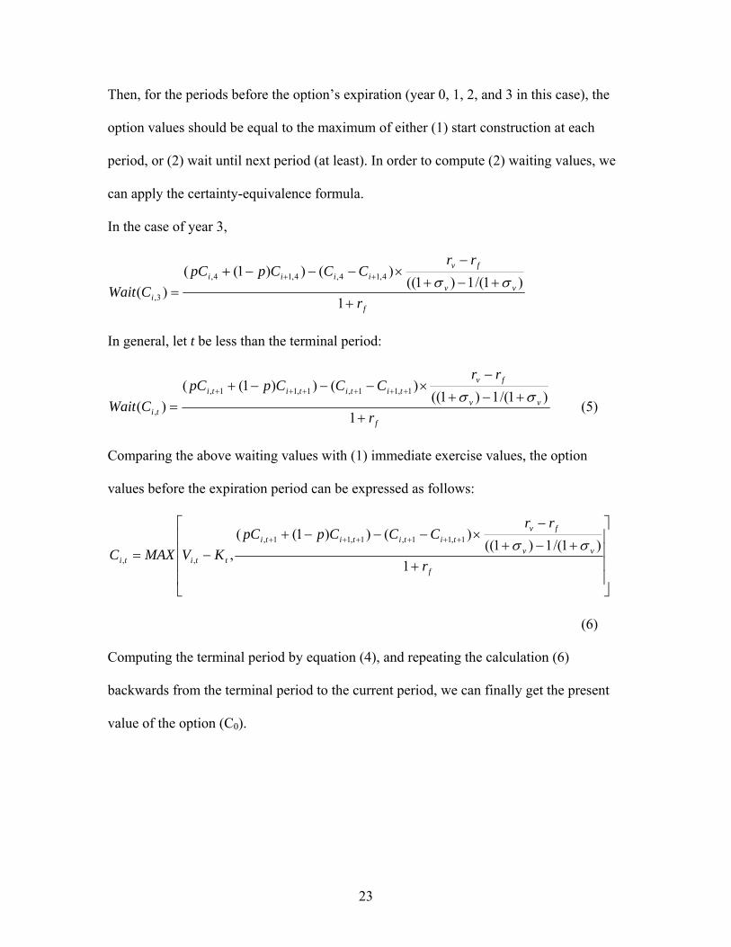
Then, for the periods before the option’s expiration (year 0, 1, 2, and 3 in this case), the

option values should be equal to the maximum of either (1) start construction at each

period, or (2) wait until next period (at least). In order to compute (2) waiting values, we

can apply the certainty-equivalence formula.

In the case of year 3,

f

vv

fviiii

i r

rrCCCppC

CWait+

+−+

−×−−−+

=++

1)1/(1)1((

)())1(()(

4,14,4,14,

3,σσ

In general, let t be less than the terminal period:

f

vv

fvtitititi

ti r

rrCCCppC

CWait+

+−+

−×−−−+

=++++++

1)1/(1)1((

)())1(()(

1,11,1,11,

,σσ

(5)

Comparing the above waiting values with (1) immediate exercise values, the option

values before the expiration period can be expressed as follows:

⎥⎥⎥⎥

⎦

⎤

⎢⎢⎢⎢

⎣

⎡

++−+

−×−−−+

−=++++++

f

vv

fvtitititi

ttiti r

rrCCCppC

KVMAXC1

)1/(1)1(()())1((

,1,11,1,11,

,,σσ

(6)

Computing the terminal period by equation (4), and repeating the calculation (6)

backwards from the terminal period to the current period, we can finally get the present

value of the option (C0).

23

3.1.2 Samuelson-McKean formula

Although the binominal option valuation method described above plays a central

role in the analysis, the method has one important weakness. As is obvious in Figure 3.1,

the binominal trees have to come to an end after some periods. That is to say, the land

development option should be finite in this method. However, more often than not, the

land development can be seen as a perpetual American call option, as I mentioned before.

In order to precisely compute this perpetual option value, Geltner et al. (2007) suggested

using the Samuelson-McKean formula.

The Samuelson-McKean formula is an example of the closed-form solutions for

real options, originally developed for pricing perpetual American warrants by Paul

Samuelson and Henry McKean in 1965. Regarding the developable land as a call option

without maturity of expiration, Geltner et al. (2007) suggest the Samuelson-McKean

formula as being suitable for valuing real estate development options than other closed-

form solutions such as the Black-Scholes equation.

Letting ηdenote the option elasticity, the Samuelson-McKean formula is given as

follows:

2

2222

222

v

vkv

vkv

kv yyyyy

σ

σσσ

η

+⎟⎟⎠

⎞⎜⎜⎝

⎛−−++−

=　 (7)

Then, assuming that the built property value (currently V0) is the highest and best use

(HBU) for the subject land, and that the construction cost (currently K0) corresponds to

the HBU, the option value can be expressed as follows:10

10 I am assuming instantaneous construction in the formula. The modification to incorporate the time to build will be discussed in the following section.

24

η

)*

)(*( 000 V

VKVC −= (8)

Where V*, the hurdle value of V which suggests the optimal timing of the immediate

exercise, is given by:

)1(* 0

−=

ηηK

V (9)

3.1.3 Time to build

As I mentioned before, I have been assuming instantaneous construction both in

the binominal option valuation method and in the Samuelson-McKean formula. However,

in order to make these methods more realistic, we need to account for the time required

between the beginning of construction and the completion of the building. Here I let “ttb”

denote the time required to build the underlying asset.

Suppose we decide to exercise the development option at time t. Then we obtain

the completed building at time (t + ttb). Therefore, in order to make decisions at time t,

we have to discount the future expected value of the building to time t, when we exercise

the option, at the risk-adjusted discount rate for the underlying asset. The present value as

of time t of the future property value completed at time (t + ttb) is calculated as follows:

[ ] [ ]ttb

v

tttb

v

ttbv

ttbv

t

ttbv

ttbvt

ttbv

ttbttttbtt y

Vryr

V

rgV

rVE

VPV)1()1(

))1()1(

(

)1()1(

)1( +=

+++

=++

=+

= ++

As for the construction cost, I assume the single lump-sum payment at the time of

completion of the building (i.e., at time (t + ttb)). Thus, the present value as of time t of

the future construction cost due at time (t + ttb) is calculated in the same way, as follows:

25

[ ] [ ]ttb

k

tttb

f

ttbk

ttbf

t

ttbf

ttbkt

ttbf

ttbttttbtt y

Kr

yr

K

rgK

rKE

KPV)1()1(

))1()1(

(

)1()1(

)1( +=

++

+

=++

=+

= ++

So far, I have used Vt and Kt to calculate the immediate exercise value in the

binominal option valuation method, and used V0 and K0 in the Samuelson-McKean

formula. In more realistic cases with the notion of time to build, we should replace Vt and

Kt with the results of PVt[Vt+ttb] and PVt[Kt+ttb], respectively. This replacement is

effective both in the binominal option valuation method and in the Samuelson-McKean

formula.

26

3.2 Engineering-based approach

There are many types of option calculation methods within the simulation

approach as well as several specialized simulation software such as Crystal Ball® and

@Risk®. However, the engineering-based model I focus on here is a relatively simple

method based on Excel® software, which could be most easily used by practicing people

in the real world. It is basically following the method developed by de Neufville et al.

(2006). Also, many aspects of the model are introduced by Cardin (2007).

The method has been developed mainly from the perspective of designers of

engineering systems, who seek to maximize the value of the systems under uncertain

future conditions. Recognizing that the difficulty of understanding financial theory and

the cost and time needed to employ a new decision method are the main reasons why the

value of flexible design is sometimes overlooked, the methodology proposes a simpler

approach to value flexibility in engineering systems, using Excel® spreadsheet. Although

this approach is very simple, it makes the best use of the computational power of Excel®

software in the analysis such as the Monte Carlo simulation as well as in the graphic

presentation of the results. The Monte Carlo simulation is used here to simulate

thousands of movements of the uncertain variable(s) by randomly and repeatedly

changing values.

To summarize, following de Neufville et al. (2006), the engineering-based

approach has three typical advantages compared to other valuation approaches:

“It uses standard, readily accessible spreadsheet procedures”

“It is based on data available in practice”

“It provides graphics that explain the results intuitively”

27

The analysis methodology consists of four steps. I describe the procedure of each step

below.

3.2.1 Step 1: Create the most likely initial cash flow pro forma

First, designers need to create an initial model based on deterministic projections

(i.e., without uncertainty). This model calculates one result such as the net present value

(NPV), which is used to measure the value and performance of the project. In contrast to

the economics-based approach, a single risk-adjusted discount rate should be assumed in

order to calculate the NPV in this step. This initial model is called the “static case” in this

thesis, and serves as a benchmark to measure the effect of uncertainty and flexibility.

The idea in this first step is to represent the decision metric typically used in the

current real-world practice. In effect, developers (and potential lenders and financiers)

currently use this type of “pro forma” decision metric, which is based on a single

projected (“expected” or “most likely”) cash flow stream for the entire project. The cash

flow stream may be discounted at a specified “hurdle rate” to arrive at an NPV or it may

be used to derive a going-in IRR for the project (which is then implicitly if not explicitly

compared to some hurdle). These two approaches are mathematically equivalent in the

present context. Indeed, developers may actually express their decision metric in even

simpler ratio terms, such as looking for a “necessary” gross margin over cost, or a

stabilized year yield (net operating income over all-in development costs). But it seems

likely that successful developers actually consider the NPV of proposed projects (or the

effectively equivalent technique of comparing the going-in IRR to a hurdle). The key

point is that this benchmark “static case” which represents the current project analysis

28

and decision making practice is based on a single (hence, effectively “deterministic”)

cash flow projection for the proposed development project.

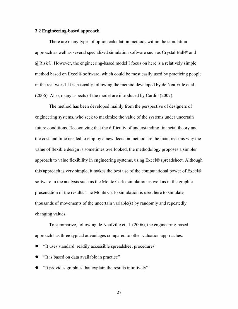
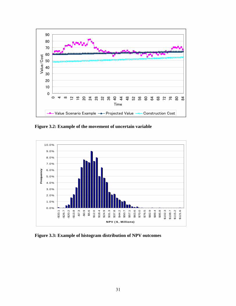
3.2.2 Step 2: Incorporate uncertain variable(s) into the initial model

Next, designers incorporate one or more uncertain variables into the initial model.

In the case of real estate development, examples of uncertain variables would be future

rents, market demand, and values of built property. Figure 3.2 shows an example of the

random movement of an uncertain variable. This random simulation of uncertain

variables can be conducted by the Monte Carlo simulation in Excel® software. Designers

can review the initial model based on several uncertain variable scenarios, and examine

how much the uncertainty affects the value and performance of the project. If we use the

NPV of the project as a criterion, the “expected net present value” (ENPV), which can be

calculated based on all possible scenarios, should be compared to the static case NPV.

The possible outcomes of the NPV can be shown in a histogram distribution, an example

of which is shown in Figure 3.3. This model with uncertainty but without flexibility is

called the “inflexible case” in this thesis.

This Monte Carlo model explicitly incorporates uncertainty into the project

analysis, but does not at this stage allow for decision flexibility. In other words, the

Monte Carlo model at this stage assumes the same project exercise parameters (what is to

be built, and when) as is assumed in the previous static case.

To be consistent with classical decision analysis methodology, all of the future

cash flow “histories” that are generated in the Monte Carlo model are discounted to

present value using the same exogenously-specified discount rate, and to be consistent we

29

must employ this same discount rate (opportunity cost of capital) in all four steps of the

engineering-based approach. Clearly, this discount rate will determine the present value

of each and every one of the simulated future “histories” and therefore will situate the

step 2 histogram of Figure 3.3 along the horizontal axis (NPV values). Thus, the ENPV

of the Monte Carlo representation of uncertainty under the projected implementation plan

for the project is determined by this exogenously-specified discount rate. To make the

engineering-based model as equivalent as possible to the economics-based model without

violating the essential simplifying features of the engineering approach, we propose to

calibrate this exogenously-specified discount rate so as to closely approximate the Monte

Carlo ENPV of Step 2 to the deterministic NPV of the Step 1 static case described in the

previous section.11 The idea is that the static case NPV well reflects the way developers

(and their financiers) currently would value the development project, and therefore well

reflects the opportunity cost of capital which they at least perceive be relevant for the

development project investment decision.

11 Under typical regularity assumptions, this will in fact be a discount rate very similar to that employed in the deterministic NPV calculation of the section 3.2.1. In fact, in the case study in Chapter 4, I will use identically the same discount rate in the two steps.

30

0

10

20

30

40

50

60

70

80

90

0 4 8 12

16

20

24

28

32

36

40

44

48

52

56

60

64

68

72

76

80

84

Time

Val

ue/

Cos

t

Value Scenario Example Projected Value Construction Cost

Figure 3.2: Example of the movement of uncertain variable

0.0%

1.0%

2.0%

3.0%

4.0%

5.0%

6.0%

7.0%

8.0%

9.0%

10.0%

-$33.1

-$26.7

-$20.2

-$13.8

-$7.3

-$0.9

$5.6

$12.0

$18.4

$24.9

$31.3

$37.8

$44.2

$50.7

$57.1

$63.6

$70.0

$76.5

$82.9

$89.4

$95.8

$102.3

$108.7

$115.2

$121.6

NPV ($, Millions)

Fre

quency

Figure 3.3: Example of histogram distribution of NPV outcomes

31

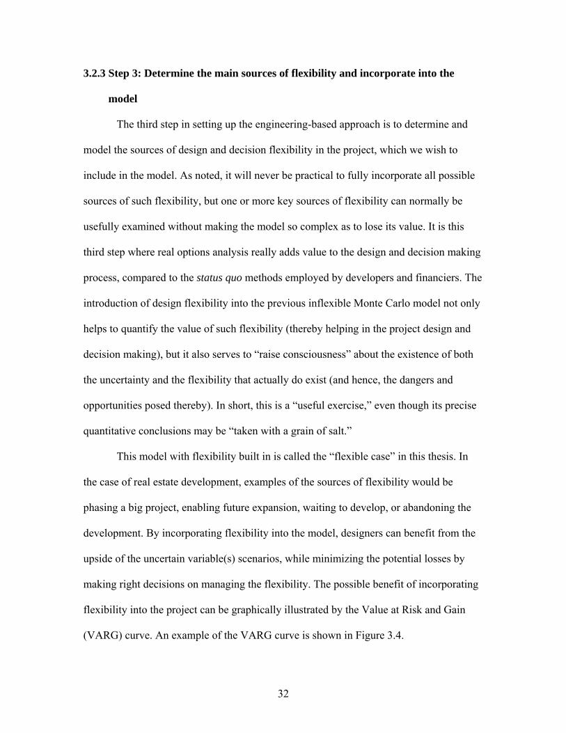
3.2.3 Step 3: Determine the main sources of flexibility and incorporate into the

model

The third step in setting up the engineering-based approach is to determine and

model the sources of design and decision flexibility in the project, which we wish to

include in the model. As noted, it will never be practical to fully incorporate all possible

sources of such flexibility, but one or more key sources of flexibility can normally be

usefully examined without making the model so complex as to lose its value. It is this

third step where real options analysis really adds value to the design and decision making

process, compared to the status quo methods employed by developers and financiers. The

introduction of design flexibility into the previous inflexible Monte Carlo model not only

helps to quantify the value of such flexibility (thereby helping in the project design and

decision making), but it also serves to “raise consciousness” about the existence of both

the uncertainty and the flexibility that actually do exist (and hence, the dangers and

opportunities posed thereby). In short, this is a “useful exercise,” even though its precise

quantitative conclusions may be “taken with a grain of salt.”

This model with flexibility built in is called the “flexible case” in this thesis. In

the case of real estate development, examples of the sources of flexibility would be

phasing a big project, enabling future expansion, waiting to develop, or abandoning the

development. By incorporating flexibility into the model, designers can benefit from the

upside of the uncertain variable(s) scenarios, while minimizing the potential losses by

making right decisions on managing the flexibility. The possible benefit of incorporating

flexibility into the project can be graphically illustrated by the Value at Risk and Gain

(VARG) curve. An example of the VARG curve is shown in Figure 3.4.

32

0%

10%

20%

30%

40%

50%

60%

70%

80%

90%

100%

-$100.0 -$50.0 $0.0 $50.0 $100.0 $150.0 $200.0 $250.0

NPV ($, Millions)

Cu

mu

lati

ve p

robabilit

y

VARG Flexible Case ENPV Flexible Case Static NPV

VARG Inflexible Case ENPV Inflexible Case

Figure 3.4: Example of Value at Risk and Gain (VARG) curve

3.2.4 Step 4: Search for the combination of decision rules to maximize value

The role of flexibility is to adapt efficiently to the uncertain variable scenarios and

to create the best results. Therefore, this step is critical in determining the value of

flexibility. Here, “decision rules” refer to the criteria for determining how to manage

flexibility. For example, in the case of real estate development, if the future rent is

uncertain, a decision rule might be: “begin the construction when the rent keeps

increasing for three consecutive years.” Supposing that designers have more than two

sources of flexibility in the project, then they need to search for the best combination of

decision rules which enables them to acquire the best result based on the entire set of the

uncertain variable scenarios. However, this final step is not an easy job, because many

33

Monte Carlo simulations are needed in order to obtain reliable results.12 Therefore, this

“maximization of the value with flexibility” often depends largely on the ability and the

expertise of project designers. Cardin (2007) proposed a useful method to attack this

problem, which is discussed in detail in the next section.

3.2.5 Scenario categorization and catalog of operating plans

Here is the method to reduce the time of examination in searching for the best

combination of decision rules in Step 4. First, the categorization of uncertain variable

scenarios is introduced in Step 2. This means that designers categorize all possible

scenarios of uncertain variables into a limited set of standardized scenarios. For example,

supposing that we run two thousand scenarios of possible future rent, then these two

thousand scenarios could be categorized into four standardized scenarios. Four categories

might be: high initial rent and high growth, high initial rent and low growth, low initial

rent and high growth, and low initial rent and low growth.

Then, in Step 4, designers search for the best combination of decision rules for

each of the standardized uncertain variable scenarios. In the above example, designers

only need to determine four combinations of decision rules to capture two thousand

scenarios. These four combinations of decision rules are called the “catalog of operating

plans.” At the final step, designers examine how much value can be added by

incorporating flexibility and using the catalog of operating plans, based on randomized

uncertain variable scenarios. For example, if the randomized rent movement is

categorized into the “low initial rent and high growth” category, designers pick up the

12 For example, two thousand simulations are conducted in the case study in Chapter 4.

34

relevant combination of decision rules, which maximizes the value of project under the

future rents in that particular category, and repeat the same procedure for all uncertain

variable scenarios.

This procedure can be easily done using Monte Carlo simulation in Excel®

software. Finally, the ENPV is calculated based on all NPVs computed in each of the two

thousand simulations. If there is the value of flexibility, the ENPV of the flexible case

must be higher than that of the inflexible case, and the difference of the two cases can be

referred to as “the value of flexibility,” in other words, “the value of real options.”

Although this methodology can considerably reduce the workload of designers,

categorization of scenarios requires the time to observe the movement of uncertain

variable(s). If we are not allowed the time for observation, as is also the condition in the

case study in Chapter 4, this method may not be well suited to searching for the best

combination of decision rules.

Findings and conclusions in a companion MIT/CRE MSRED thesis suggest that

in the typical real estate development context, the type of formal searching for the

optimal combination of decision rules probably adds too much complexity to the real

options analysis. Most developers can usually heuristically or intuitively identify the

major important sources of uncertainty and decision flexibility possibilities, for a typical

real estate development project. So it is not necessary to introduce formal cataloguing and

optimizing of such decision rules in the real estate development application of real

options analysis. This finding is in some contrast to typical cases in complex engineering

system applications.13

13 See and compare the previously noted Cardin (2007) and Barman & Nash (2007).

35

3.3 Common issues in both models

Here I describe four issues that are important in valuing real options both in the

economics-based approach and in the engineering-based approach. These four issues are:

Risk-neutral probability approach vs. “real” probability approach

Compound options

Choice of uncertain variable(s)

Movement of uncertain variable(s)

3.3.1 Risk-neutral probability approach vs. “real” probability approach

It should be noted that not only the engineering-based approach but also the

economics-based approach I addressed above are based on the “real” probability

approach, which should be distinguished from the risk-neutral probability approach that

is more commonly used in economic applications, including in the binominal option

valuation model.

The primary advantage of using the risk-neutral probability approach is that we do

not need to make an assumption on the risk-adjusted discount rate, and that we can

simply use the risk-free rate of interest. However, since it mathematically modifies up

and down probabilities so that cash flows can be discounted at the risk-free rate, it is

often difficult for practitioners to understand the method intuitively. Also, since the

probabilities are not “true” probabilities related to the actual expected movement of the

underlying asset, it is sometimes confusing to illustrate the movement graphically.

There is also a communication issue with the risk-neutral approach. Real estate

developers are actually aware of risk, and that they themselves are very much not “risk-

36

neutral.” It can make it difficult to communicate to them the usefulness of the real options

analysis approach if one has to explain that the analysis is done as though the world were

risk-neutral even though we all know it really is not. We risk “losing the audience,” so to

speak, among the decision-makers who must actually apply real options analysis if it is to

have an influence in the real world.

In this thesis, instead, I primarily use the “real” probability approach. In the

binominal option valuation model, I use the “real” probability approach along with the

certainty-equivalence approach. Discounting future cash flows should account for the

time value of money and the risk premium. By applying the certainty-equivalence

formula, we can “risk-adjust” cash flows which are based on “real” probabilities, and

discount the calculated “certainty-equivalent value” at the risk-free rate to adjust it for the

time value of money.14

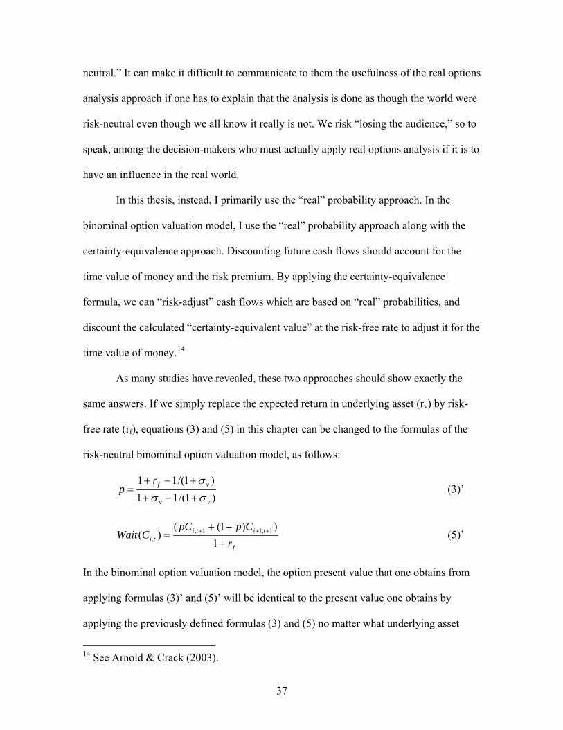
As many studies have revealed, these two approaches should show exactly the

same answers. If we simply replace the expected return in underlying asset (rv) by risk-

free rate (rf), equations (3) and (5) in this chapter can be changed to the formulas of the

risk-neutral binominal option valuation model, as follows:

)1/(11)1/(11

vv

vfrp

σσσ

+−+

+−+= (3)’

f

tititi r

CppCCWait

+

−+= +++

1))1((

)( 1,11,, (5)’

In the binominal option valuation model, the option present value that one obtains from

applying formulas (3)’ and (5)’ will be identical to the present value one obtains by

applying the previously defined formulas (3) and (5) no matter what underlying asset

14 See Arnold & Crack (2003).

37

OCC rate (rv) one employs. The option value is indeed independent of the expected return

of the underlying asset. The reasons I apply “real” probability approach are that it is

easier to show the expected movement of the values of underlying asset and option, and

that it is the better way to compare with the engineering-based approach, which is also

based on the risk-adjusted discount rates in this thesis.

3.3.2 Compound options

The “compound options” or “options on options” is referred to as options whose

value is dependent on other options. There are two types of compound options:

simultaneous compound options and sequential compound options. In the case of real

estate development, a multi-phased development project can be seen as an example of the

sequential compound options model. Simply thinking of the two-phased real estate

development project, the second phase can be initiated only when the first phase is

already built. In other words, the exercise of the first phase option includes the

acquisition of the second phase option.

In order to precisely calculate the value of sequential compound options in the

binominal option valuation method, we need to think about the value of options in

reverse chronological order. That is to say, we first calculate the value of the second

phase option, and then judge the exercise of the first phase option taking into account the

present value of the second phase option. This issue will be examined in the case study in

Chapter 4.

38

3.3.3 Choice of uncertain variable(s)

In this section, I examine the issue of choosing uncertain variable(s), focusing on

the case of real estate development. This issue is very important in evaluating the value of

flexibility, since the uncertainty is the indispensable component of the value of flexibility.

In other words, there would be no value of flexibility without any uncertainty in the

project.

In the case of real estate development, it may be intuitively more natural for

practitioners to set volatility in future rents and cap rates. However, regarding this issue,

Copeland and Antikarov (2003) introduced the theory originally proved by Paul

Samuelson in 1965. The implication of the theory is that even when there are more than

two uncertain variables that drive the value of the underlying asset, those uncertainties

can be combined into a single uncertainty in the value of the underlying asset, and that

the value of the underlying asset shows a normal “random walk” over time with a

constant volatility, regardless of the movement of cash flows driven by other

uncertainties. Also, the more variables that are incorporated into the model, the more

complicated the calculation will be. Therefore, I use the value of built property

(underlying asset of the land option) as a single uncertain variable, which can integrate

the effect of rents and cap rates at the same time.

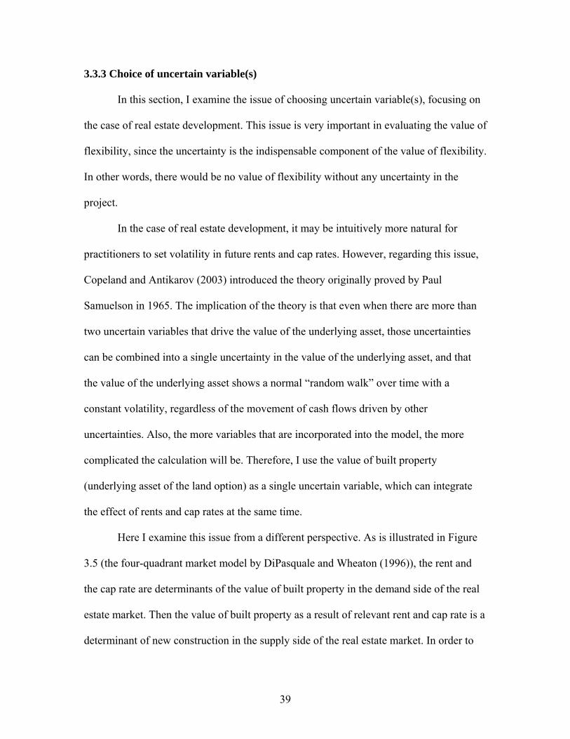
Here I examine this issue from a different perspective. As is illustrated in Figure

3.5 (the four-quadrant market model by DiPasquale and Wheaton (1996)), the rent and

the cap rate are determinants of the value of built property in the demand side of the real

estate market. Then the value of built property as a result of relevant rent and cap rate is a

determinant of new construction in the supply side of the real estate market. In order to

39

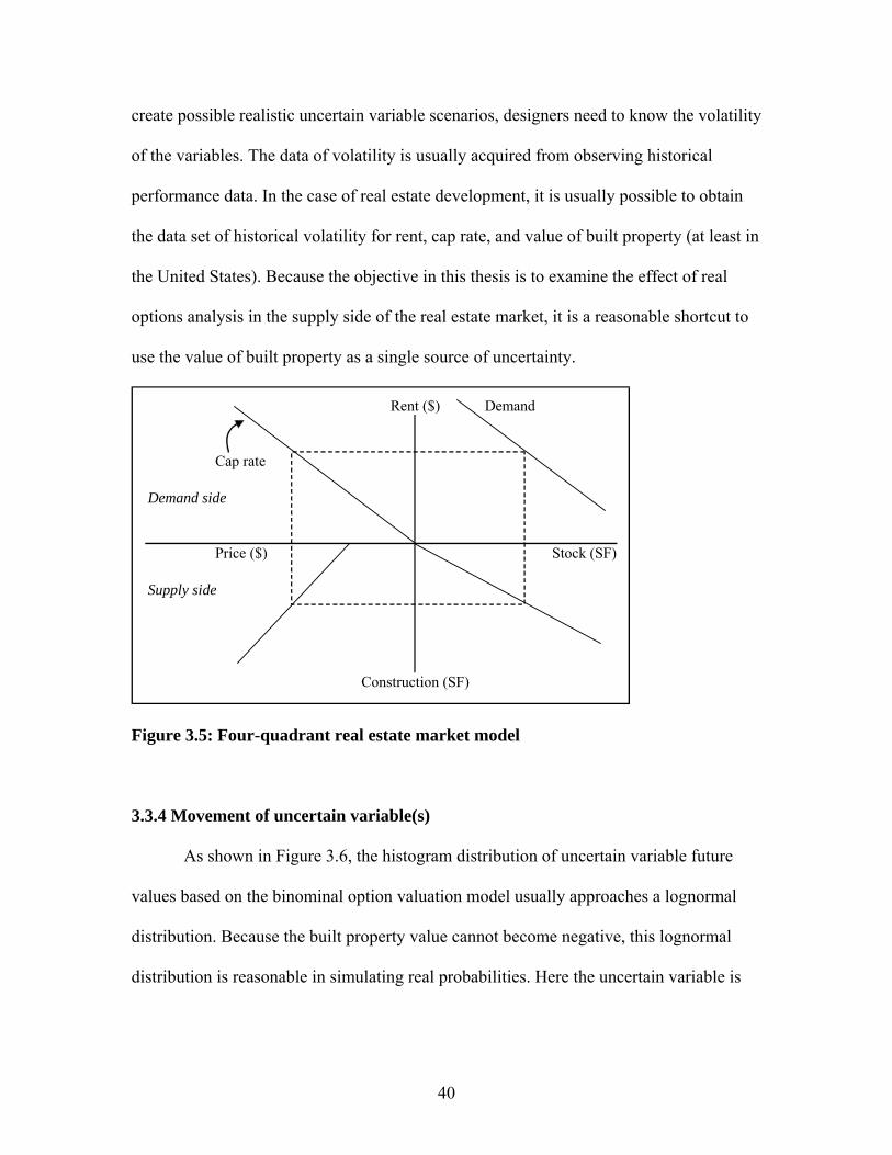
create possible realistic uncertain variable scenarios, designers need to know the volatility

of the variables. The data of volatility is usually acquired from observing historical

performance data. In the case of real estate development, it is usually possible to obtain

the data set of historical volatility for rent, cap rate, and value of built property (at least in

the United States). Because the objective in this thesis is to examine the effect of real

options analysis in the supply side of the real estate market, it is a reasonable shortcut to

use the value of built property as a single source of uncertainty.

Rent ($) Demand

Cap rate

Demand side

Price ($) Stock (SF)

Supply side

Construction (SF)

Figure 3.5: Four-quadrant real estate market model

3.3.4 Movement of uncertain variable(s)

As shown in Figure 3.6, the histogram distribution of uncertain variable future

values based on the binominal option valuation model usually approaches a lognormal

distribution. Because the built property value cannot become negative, this lognormal

distribution is reasonable in simulating real probabilities. Here the uncertain variable is

40

supposed to follow the movement known as the “random walk,” and this process is called

“stochastic process,” or “Geometric Brownian Motion.”

In Geometric Brownian Motion, the process of an uncertain variable is expressed

as follows:

εσα ~ttSS

Δ+Δ=Δ

where S is the value of the uncertain variable, ΔS is the change of that value, α is the

constant expected return (drift rate), σ is the constant instantaneous standard deviation of

returns, Δt is the time step, and ε is a random sample from a standardized normal

distribution.

To replicate this motion in the engineering-based model, I create the movement

with the standard-normal distribution of mean zero and a variance of one by the

following formula in the Excel® software:

)())(1(1 dtRANDNORMSINVSS tt σα ∗++×= −

41

0.0%

2.0%

4.0%

6.0%

8.0%

10.0%

12.0%

14.0%

16.0%

18.0%

472.

42

410.

96

357.

50

310.

99

270.

54

235.

34

204.

73

178.

09

154.

92

134.

77

117.

24

101.

99

88.7

2

77.1

8

67.1

4

58.4

0

50.8

1

44.2

0

38.4

5

33.4

4

29.0

9

25.3

1

22.0

2

19.1

5

16.6

6

Value of uncertain variable

Freq

uenc

y

Figure 3.6: Example of histogram distribution of future values of uncertain

variable

42

Chapter 4 Case Study

In this chapter, I attempt a detailed comparison between the economics-based

approach and the engineering-based approach. I use a real estate development case study,

which is called the “Roth Harbor” case. This case study is developed and introduced in

Geltner et al. (2007). The authors have created a real options valuation model based on

the binominal tree option valuation method in Appendix 29 of their book. Here I will

develop an engineering-based real options model for this case and review the economics-

based model so that I can rigorously compare these two models. The goal of this chapter

is to examine in depth the main difference between the two models, and to propose the

possibility, if any, of making the engineering-based model more reliable in comparison

with the economics-based model. (The rationale for using the economics-based approach

as the development project valuation benchmark is that the economics-based approach is

based rigorously on equilibrium theory, as noted previously, and therefore has a

fundamental rationale for equating its valuation to a normative or market-based

opportunity cost (or value) for the development project.)

4.1 Case statement

Roth Harbor is located in a former brown-field site near the center of a city in the

United States. Currently plenty of people are moving into the city, and the city is running

short of housing. The 50-acre Roth Harbor site is currently zoned to allow 500 units of

market-rate apartments. The current owner of the site is planning to build 500 units of

apartments as a single-phase project, which is called Rentleg Gardens.15 However, the

15 The site is assumed to have been made ready for development by the current owner.

43

planning commission of the city has another idea, which is called Roth Harbor Place

(RHP). This alternative idea is based on a special zoning exemption, which allows

another (or current) developer to develop more units than the current zoning limitation

allows. In return, the developer should also provide approximately 25% of units as

affordable housing in a two-phased development, called Phase I and Phase II,

respectively. The assumptions of Rentleg Gardens and RHP are summarized in Table 4.1.

Even though the market demand and the risk-return profile could differ between market

rent units and affordable units, the same rates of gk, yv, rv, and σv are assumed here for

simplicity. Therefore, all the projected development plans have the same dynamics in

terms of the value of built property.

Table 4.1: Assumptions of Roth Harbor case

Rentleg Gardens Roth Harbor PlacePhase I Phase II

# of Unit 500 900 1600Current NOI (annual) $3,200,000 $4,800,000 $8,000,000Current Built Property Value (V0) $40,000,000 $60,000,000 $100,000,000Current Construction Cost (K0) $32,000,000 $48,000,000 $80,000,000Construction Period (time to build) 12 months 24 months 24 monthsDeadline to Build (from now) Perpetual 36 months 60 monthsConstruction Cost Growth Rate (gk) 2.0% /yearCap Rate (yv) 8.0%Market OCC for Stabilized Asset (rv) 9% /yearRisk-free Interest Rate (rf) 4%Volatility of Built Property (σv) 15% /year

* All annual rates are monthly compounding, annual percentage rates.

Phase I of the RHP can be developed at any time between now and 36 months

from now, which means that developing Phase I is an American call option. Phase II of

the RHP is also an American call option, which can be exercised at any time within 60

44

months from now, but only after Phase I has been developed (and completed). Therefore,

the RHP project is characterized as a compound option, where the underlying asset of the

Phase I option includes the option of Phase II.

If the developer finds the RHP project unprofitable, he can abandon the right of

special zoning exemption at any time within 36 months and sell the land based on the as-

of-right Rentleg Gardens development value. In this sense, this alternative development

can be regarded as an “abandonment option” from the perspective of the RHP

developer.16 It should be noted that even if Phase II is not developed after Phase I

completion, the land has simply the value of the built property of Phase I, since Phase I

development itself exceeds the as-of-right zoning allowance. To summarize, the possible

results of this case study are either (1) develop Phase I and Phase II of the RHP, (2)

develop Phase I of the RHP only, or (3) abandon the RHP and obtain the as-of-right land

value based on the development of Rentleg Gardens.

16 This “abandonment option” is an option in a broad sense (not exactly a typical put option), since the exercise price is not given in advance.

45

4.2 Economics-based approach

Here I review the real options value in the Roth Harbor case based on the

economics-based approach. I use the result of this method as a valuation benchmark to be

compared with the engineering-based approach. That is to say, I assume this rigorous

approach can always calculate the “true” real options value. In order to attempt a detailed

comparison with the engineering-based approach, I extend the binominal trees from

annual base to monthly base, assuming all assumptions of annual rates as monthly

compounding annual percentage rates.

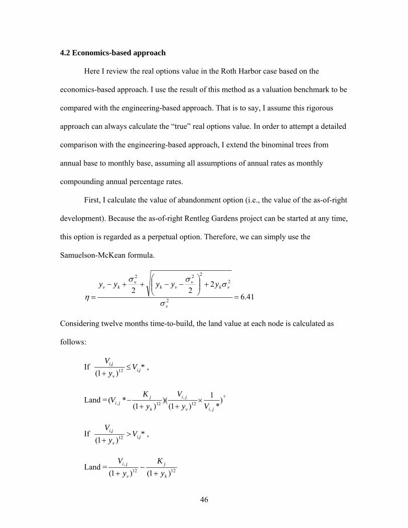
First, I calculate the value of abandonment option (i.e., the value of the as-of-right

development). Because the as-of-right Rentleg Gardens project can be started at any time,

this option is regarded as a perpetual option. Therefore, we can simply use the

Samuelson-McKean formula.

41.62

22　 2

2222

=

+⎟⎟⎠

⎞⎜⎜⎝

⎛−−++−

=v

vkv

vkv

kv yyyyy

σ

σσσ

η

Considering twelve months time-to-build, the land value at each node is calculated as

follows:

If *Vy

Vi,j

v

i,j ≤+ 12)1(

,

Land =η

)*

1)1(

)()1(

*(,

12,

12,jiv

ji

k

jji Vy

Vy

KV ×

++−

If *Vy

Vi,j

v

i,j >+ 12)1(

,

Land = 1212,

)1()1( k

j

v

ji

yK

yV

+−

+

46

where

185.1)1()1()1(

)1(* 1212

12

, ×+

=−

×++

×=v

j

f

kjji r

KrgKV

ηη

Repeating the above calculation, the binominal tree of the land price based on the as-of-

right Rentleg Gardens is given in Table 4.2. This tree is used as an abandonment value

tree in the analysis of the RHP project.

Table 4.2: Rentleg Gardens project land value tree (only the first 12 months are

shown to conserve space.) Rentleg Gardens Land Value Tr ee (Samuelson-McKean, reflecting 12 month time-to-build):

Month ("j "): 0 1 2 3 4 5 6 7 8 9 10 11"down" moves ("i"):

0 5.65 6.96 8.31 9.72 11.18 12.69 14.26 15.89 17.59 19.34 21.17 23.06 25.021 4.10 5.12 6.36 7.70 9.09 10.53 12.02 13.57 15.18 16.85 18.59 20.392 2.97 3.71 4.63 5.78 7.10 8.46 9.88 11.36 12.89 14.48 16.133 2.16 2.69 3.36 4.19 5.23 6.50 7.85 9.25 10.70 12.214 1.56 1.95 2.43 3.04 3.79 4.73 5.90 7.24 8.5 1.13 1.41 1.76 2.20 2.75 3.43 4.28 5.346 0.82 1.03 1.28 1.60 1.99 2.49 3.107 0.60 0.74 0.93 1.16 1.44 1.808 0.43 0.54 0.67 0.84 1.059 0.31 0.39 0.49 0.6110 0.23 0.28 0.3511 0.16 0.2112 0.12

12

62

Next, considering that the RHP Phase I is a compound option including the option

value of the RHP Phase II, we first build the binominal trees of RHP Phase II. This work

can be done in the way I discussed in Chapter 3. That is to say, build the underlying asset

value tree, build the corresponding construction cost tree, and build the option value tree

working backward using the certainty-equivalence formula from month 60 (option’s

expiration period) to month 0.

Then, before building the binominal trees of the RHP Phase I, we should take into

account that the option of the RHP Phase II can only be exercised after 24 months of the

option exercise of the RHP Phase I. To include the option value of the RHP Phase II as a

47

part of the RHP Phase I compound option, the option value of Phase II should be

calculated back 24 months to be the present value as of the time when the Phase I option

may be exercised. To conduct this calculation, we can use the certainty-equivalence

formula again. Table 4.3 shows the tree of the present values of the RHP Phase II option

as of the time when Phase I may be exercised.

Table 4.3: Present value of 24 months delayed receipt of the RHP Phase II option

value (only the first 12 months are shown to conserve space.) PV of 24 period delayed receipt of Phase II option value:

Month ("j "): 0 1 2 3 4 5 6 7 8 9 10 11"down" moves ("i"):

0 6.87 8.29 9.93 11.76 13.82 16.11 18.60 21.33 24.26 27.40 30.74 34.28 38.021 5.11 6.27 7.60 9.14 10.89 12.85 15.05 17.45 20.08 22.93 25.98 29.262 3.72 4.62 5.69 6.95 8.39 10.06 11.92 14.02 16.34 18.86 21.643 2.64 3.33 4.17 5.15 6.33 7.69 9.25 11.03 13.02 15.264 1.83 2.34 2.97 3.74 4.65 5.74 7.02 8.48 10.5 1.23 1.60 2.06 2.64 3.34 4.18 5.19 6.396 0.81 1.07 1.39 1.81 2.33 2.96 3.747 0.51 0.69 0.92 1.21 1.58 2.058 0.32 0.43 0.58 0.78 1.049 0.19 0.26 0.36 0.4910 0.11 0.15 0.2111 0.06 0.0912 0.03

12

18

Finally, we can build the binominal trees of the RHP Phase I. At the option

expiration period (month 36), the option value is the maximum of either: (1) the as-of-

right land value (Rentleg Gardens land value) or (2) immediate exercise of the RHP

Phase I compound option, including the present value of Phase II option value. At the

earlier periods from month 35 to month 0, the option value can be given by the maximum

of either: (1) the as-of-right land value (Rentleg Gardens land value), (2) immediate

exercise of RHP Phase I compound option, including the present value of Phase II option

value, or (3) holding the option unexercised until the next period (calculated by the

certainty-equivalence formula). This procedure gives the tree of the RHP Phase I option

value as shown in Table 4.4.

48

Table 4.4: Option value of the RHP Phase I (only the first 12 months are shown to

conserve space.) Value of Option on Phase I (Frenchman Cove), reflecting 24 month time-to-build:

Month ("j "): 0 1 2 3 4 5 6 7 8 9 10 11"down" moves ("i"):

0 12.14 15.37 18.88 22.67 26.74 31.13 35.80 40.79 46.07 51.64 57.52 63.67 70.131 8.37 10.78 13.85 17.23 20.91 24.86 29.13 33.69 38.55 43.71 49.17 54.942 5.73 7.42 9.59 12.37 15.64 19.20 23.04 27.17 31.61 36.34 41.403 3.88 5.04 6.55 8.48 10.95 14.09 17.53 21.25 25.26 29.594 2.60 3.40 4.43 5.77 7.50 9.73 12.59 15.90 19.525 1.73 2.26 2.96 3.87 5.06 6.60 8.58 11.146 1.15 1.50 1.96 2.57 3.37 4.42 5.797 0.76 0.99 1.29 1.70 2.23 2.928 0.51 0.66 0.85 1.11 1.469 0.34 0.44 0.57 0.7310 0.24 0.30 0.3811 0.17 0.2112 0.12

12

The current value of the option is $12.14M, which is equal to the immediate

exercise value of the RHP Phase I plus the present value of the RHP Phase II option. This

result shows that it is optimal to start the construction of the RHP Phase I now. Also, the

model tells us that this total option value is composed of the immediate exercise value of

the RHP Phase I only ($5.27M) plus the RHP Phase II option value ($6.87M). In this way,

the economics-based approach can show not only the value of real options, but also when

it is optimal for developers to start the construction. Table 4.5 is the binominal tree which

indicates the optimal decision at each node of the option tree.

Table 4.5: RHP Phase I option optimal decision tree (only the first 12 months are

shown to conserve space.) RHP Phase I Optimal Exercise :

Month ("j "): 0 1 2 3 4 5 6 7 8 9 10 11"down" moves ("i"):

0 exer exer exer exer exer exer exer exer exer exer exer exer exer1 hold hold exer exer exer exer exer exer exer exer exer exer2 hold hold hold exer exer exer exer exer exer exer exer3 hold hold hold hold hold exer exer exer exer exer4 hold hold hold hold hold hold exer exer exer5 hold hold hold hold hold hold hold exer6 hold hold hold hold hold hold hold7 hold hold hold hold hold hold8 hold hold hold hold hold9 hold hold hold hold10 hold hold hold11 hold hold12 hold

12

49

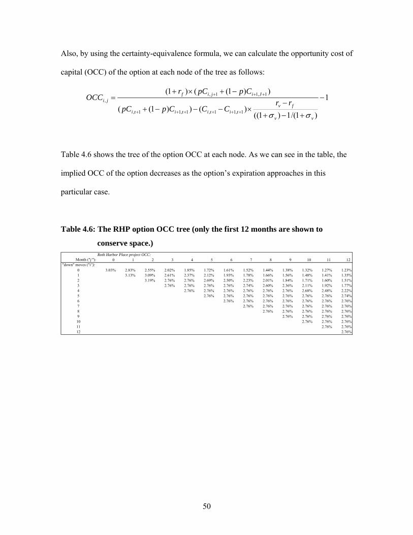
Also, by using the certainty-equivalence formula, we can calculate the opportunity cost of

capital (OCC) of the option at each node of the tree as follows:

1

)1/(1)1(()())1((

))1(()1(

1,11,1,11,

1,11,, −

+−+

−×−−−+

−+×+=

++++++

+++

vv

fvtitititi

Jijifji rr

CCCppC

CppCrOCC

σσ

Table 4.6 shows the tree of the option OCC at each node. As we can see in the table, the

implied OCC of the option decreases as the option’s expiration approaches in this

particular case.

Table 4.6: The RHP option OCC tree (only the first 12 months are shown to

conserve space.) Roth Harbor Place project OCC:

Month ("j "): 0 1 2 3 4 5 6 7 8 9 10 11"down" moves ("i"):

0 3.03% 2.83% 2.55% 2.02% 1.85% 1.72% 1.61% 1.52% 1.44% 1.38% 1.32% 1.27% 1.23%1 3.13% 3.09% 2.61% 2.37% 2.12% 1.93% 1.78% 1.66% 1.56% 1.48% 1.41% 1.35%2 3.19% 2.76% 2.76% 2.69% 2.50% 2.23% 2.01% 1.84% 1.71% 1.60% 1.51%3 2.76% 2.76% 2.76% 2.76% 2.74% 2.60% 2.36% 2.11% 1.92% 1.77%4 2.76% 2.76% 2.76% 2.76% 2.76% 2.76% 2.68% 2.48% 2.22%5 2.76% 2.76% 2.76% 2.76% 2.76% 2.76% 2.76% 2.74%6 2.76% 2.76% 2.76% 2.76% 2.76% 2.76% 2.76%7 2.76% 2.76% 2.76% 2.76% 2.76% 2.76%8 2.76% 2.76% 2.76% 2.76% 2.76%9 2.76% 2.76% 2.76% 2.76%10 2.76% 2.76% 2.76%11 2.76% 2.76%12 2.76%

12

50

4.3 Engineering-based approach

Next, I conduct the engineering-based approach following the four steps

addressed in Chapter 3. All assumptions are exactly the same as set in the previous

economics-based approach. The most critical point in the engineering-based approach is

the assumption of a single risk-adjusted discount rate. To observe this issue in depth, I

divide the analyses into two experiments as described below.

The first experiment simply assumes that the current players in the market

implicitly incorporate the value of the real options, and they could pay exactly the same

land value calculated by the economics-based approach, without recognizing flexibility in

the project. The second experiment also assumes the land purchase price in the same way,

but modifies the assumption of the volatility of built property value from 15% per annum

to 25% per annum, in order to examine the model more deeply.

4.3.1 Experiment 1

Step1: Create static case

Basic DCF analysis starts from finding the best way to maximize NPV under no

uncertainty. In Figure 4.1 and Figure 4.2, the expected built property value and the

expected construction cost of the RHP Phase I and Phase II are illustrated. Considering

the time to build of each phase (24 months), the value and the cost are shown from month

24 to 60 for Phase I, and from month 48 to 84 for Phase II, respectively. The profit

between the value and the cost decreases over time in both phases. This is a natural

outcome considering the difference of growth rate of 0.93% per annum for built property

value, and 2.0% per annum for construction cost. Therefore, a reasonable assumption of

51

maximizing profit would be to start both phases as soon as possible. That is to say, start

Phase I now and start Phase II at month 24.

40

45

50

55

60

6524

26

28

30

32

34

36

38

40

42

44

46

48

50

52

54

56

58

60

T ime (months)

($,

Millions)

Phase I Built Property Value Phase I Development Cost

Figure 4.1: Expected built property value and expected construction cost of the

RHP Phase I in static case

707580859095

100105110

48 51 54 57 60 63 66 69 72 75 78 81 84

Time (months)

($,

Millions)

Phase II Built Property Value Phase II Development Cost

Figure 4.2: Expected built property value and expected construction cost of the

RHP Phase II in static case

As for the abandonment option (Rentleg Gardens), the value at each period is

calculated using the Samuelson-McKean formula. Although I am trying to keep the

52

engineering-based approach free from the need for understanding difficult financial

theories, this formula is necessary for the fair comparison of the two models, and the

Samuelson-McKean formula is relatively easy to implement in practice. As illustrated in

Figure 4.3, the abandonment value also decreases over time from now to month 36.

4.6

4.8

5.0

5.2

5.4

5.6

5.8

0 2 4 6 8 10 12 14 16 18 20 22 24 26 28 30

Time (months)

($,

Millions)

Rentleg Abandonment Value

Figure 4.3: Expected abandonment value in static case

In this experiment, I assume that the developer would pay $12.14M for the land,

equal to the value calculated by the economics-based approach. From the above

observation, this value should be obtained by immediate exercises of Phase I and Phase II.

As shown in Figure 4.4, the implied discount rate is 2.322% per month (31.71% per

annum). This discount rate is assumed through all steps in this experiment.

53

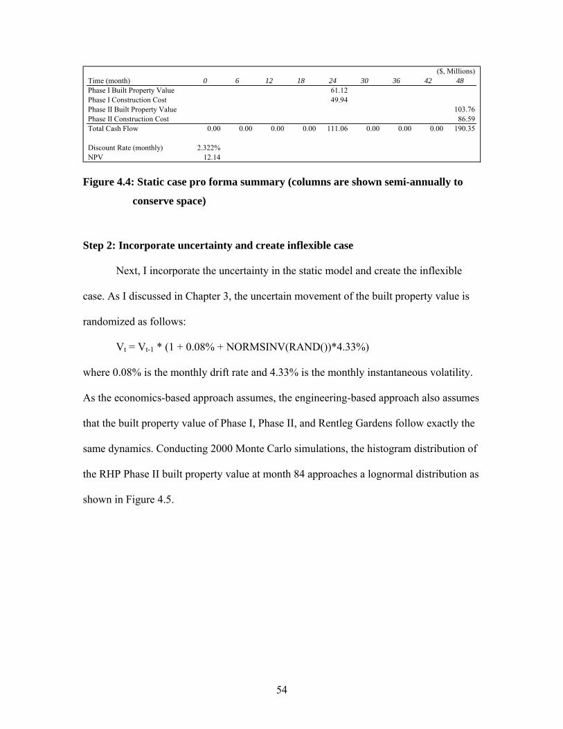
($, Millions)Time (month) 0 6 12 18 24 30 36 42 48Phase I Built Property Value 61.12Phase I Construction Cost 49.94Phase II Built Property Value 103.76Phase II Construction Cost 86.59Total Cash Flow 0.00 0.00 0.00 0.00 111.06 0.00 0.00 0.00 190.35

Discount Rate (monthly) 2.322%NPV 12.14

Figure 4.4: Static case pro forma summary (columns are shown semi-annually to

conserve space)

Step 2: Incorporate uncertainty and create inflexible case

Next, I incorporate the uncertainty in the static model and create the inflexible

case. As I discussed in Chapter 3, the uncertain movement of the built property value is

randomized as follows:

Vt = Vt-1 * (1 + 0.08% + NORMSINV(RAND())*4.33%)

where 0.08% is the monthly drift rate and 4.33% is the monthly instantaneous volatility.

As the economics-based approach assumes, the engineering-based approach also assumes

that the built property value of Phase I, Phase II, and Rentleg Gardens follow exactly the

same dynamics. Conducting 2000 Monte Carlo simulations, the histogram distribution of

the RHP Phase II built property value at month 84 approaches a lognormal distribution as

shown in Figure 4.5.

54

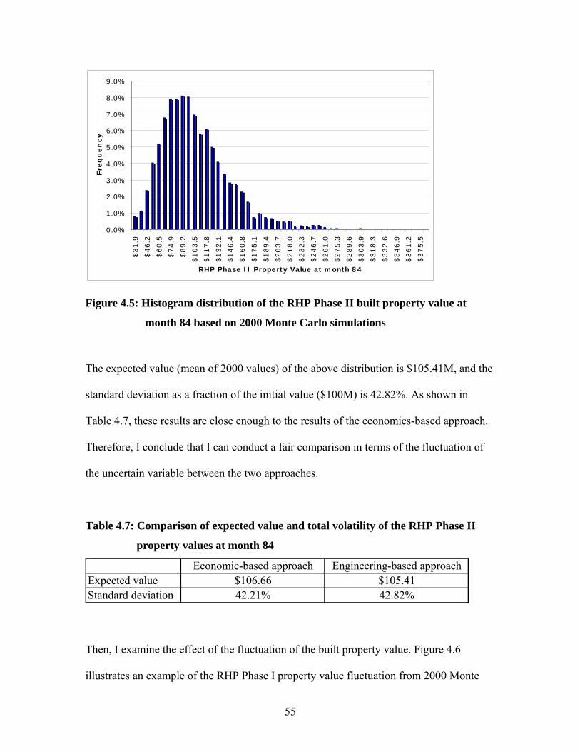
0.0%

1.0%

2.0%

3.0%

4.0%

5.0%

6.0%

7.0%

8.0%

9.0%

$31.9

$46.2

$60.5

$74.9

$89.2

$103.5

$117.8

$132.1

$146.4

$160.8

$175.1

$189.4

$203.7

$218.0

$232.3

$246.7

$261.0

$275.3

$289.6

$303.9

$318.3

$332.6

$346.9

$361.2

$375.5

RHP Phase II Property Value at month 84

Fre

qu

en

cy

Figure 4.5: Histogram distribution of the RHP Phase II built property value at

month 84 based on 2000 Monte Carlo simulations

The expected value (mean of 2000 values) of the above distribution is $105.41M, and the

standard deviation as a fraction of the initial value ($100M) is 42.82%. As shown in

Table 4.7, these results are close enough to the results of the economics-based approach.

Therefore, I conclude that I can conduct a fair comparison in terms of the fluctuation of

the uncertain variable between the two approaches.

Table 4.7: Comparison of expected value and total volatility of the RHP Phase II

property values at month 84

Economic-based approach Engineering-based approachExpected value $106.66 $105.41Standard deviation 42.21% 42.82%

Then, I examine the effect of the fluctuation of the built property value. Figure 4.6

illustrates an example of the RHP Phase I property value fluctuation from 2000 Monte

55

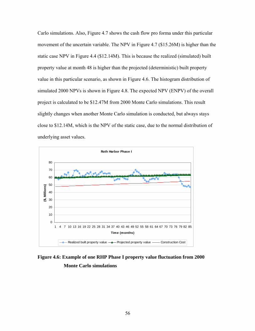
Carlo simulations. Also, Figure 4.7 shows the cash flow pro forma under this particular

movement of the uncertain variable. The NPV in Figure 4.7 ($15.26M) is higher than the

static case NPV in Figure 4.4 ($12.14M). This is because the realized (simulated) built

property value at month 48 is higher than the projected (deterministic) built property

value in this particular scenario, as shown in Figure 4.6. The histogram distribution of

simulated 2000 NPVs is shown in Figure 4.8. The expected NPV (ENPV) of the overall

project is calculated to be $12.47M from 2000 Monte Carlo simulations. This result

slightly changes when another Monte Carlo simulation is conducted, but always stays

close to $12.14M, which is the NPV of the static case, due to the normal distribution of

underlying asset values.

Roth Harbor Phase I

0

10

20

30

40

50

60

70

80

1 4 7 10 13 16 19 22 25 28 31 34 37 40 43 46 49 52 55 58 61 64 67 70 73 76 79 82 85

Time (months)

($, M

illio

ns)

Realized built property value Projected property value Construction Cost

Figure 4.6: Example of one RHP Phase I property value fluctuation from 2000

Monte Carlo simulations

56

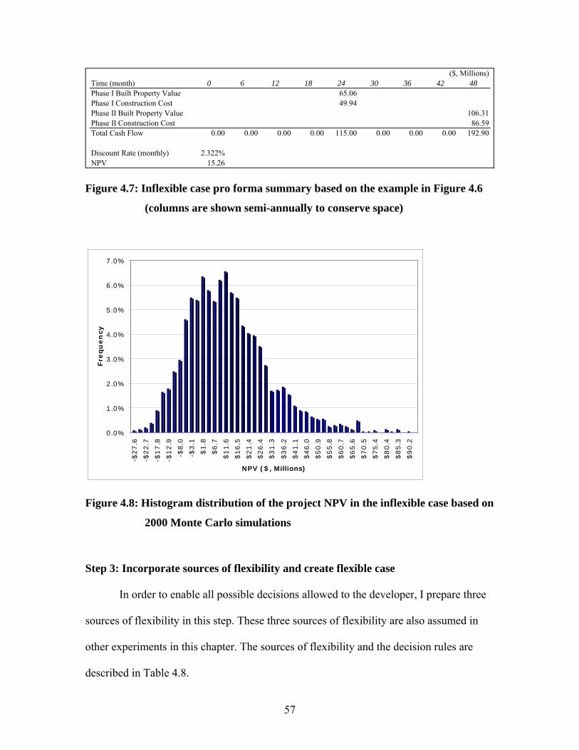
($, Millions)Time (month) 0 6 12 18 24 30 36 42 48Phase I Built Property Value 65.06Phase I Construction Cost 49.94Phase II Built Property Value 106.31Phase II Construction Cost 86.59Total Cash Flow 0.00 0.00 0.00 0.00 115.00 0.00 0.00 0.00 192.90

Discount Rate (monthly) 2.322%NPV 15.26

Figure 4.7: Inflexible case pro forma summary based on the example in Figure 4.6

(columns are shown semi-annually to conserve space)

0.0%

1.0%

2.0%

3.0%

4.0%

5.0%

6.0%

7.0%

-$27.6

-$22.7

-$17.8

-$12.9

-$8.0

-$3.1

$1.8

$6.7

$11.6

$16.5

$21.4

$26.4

$31.3

$36.2

$41.1

$46.0

$50.9

$55.8

$60.7

$65.6

$70.5

$75.4

$80.4

$85.3

$90.2

NPV ($, Millions)

Fre

qu

en

cy

Figure 4.8: Histogram distribution of the project NPV in the inflexible case based on

2000 Monte Carlo simulations

Step 3: Incorporate sources of flexibility and create flexible case

In order to enable all possible decisions allowed to the developer, I prepare three

sources of flexibility in this step. These three sources of flexibility are also assumed in

other experiments in this chapter. The sources of flexibility and the decision rules are

described in Table 4.8.

57

Table 4.8: Sources of flexibility and decision rules17

Source of flexibility Examined level Description of decision rule

When to start RHP Phase I A% If the expected benefit of Phase I is above A% ofabandonment value, start construction of Phase I

When to abandon RHP B% If the expected benefit of Phase I is below B% ofabandonment value, abandon RHP project

When to start RHP Phase II C If the expected Value/Cost ratio (V/K) is over C, startconstruction of Phase II

Step 4: Search for the best combination of decision rules and maximize NPV

As I discussed in Chapter 3, this step must be more or less dependent on the

ability and expertise of project designers. However, it is not so difficult in this particular

case to find the approximate best combination of decision rules.

First, I fix decision rule 1 and decision rule 2 in order to always assume the

immediate exercise of the RHP Phase I, as shown in Table 4.9, trials 1 to 4. Since the

currently expected exercise profit of the RHP Phase I is $5.27M and the abandonment

value as of now is $5.65M, setting decision rule 1 to 90% results in the immediate

exercise of the Phase I option in all simulated scenarios. Next, I vary decision rule 3 and

find the best level of this decision rule. As a benchmark of the level of decision rule 3, I

propose to use the Samuelson-McKean formula again. Although the RHP Phase II is a

finite call option, we can calculate the hurdle value/cost ratio assuming as if it were

perpetual. Using equation (9) in Chapter 3, the hurdle value/cost ratio is given by the

following:

185.1)141.6(

41.6)1(

*

0

=−

=−

=ηη

KV

17 It should be noted that all “expected” value and cost should take into account the notion of “time to build” in Table 4.8.

58

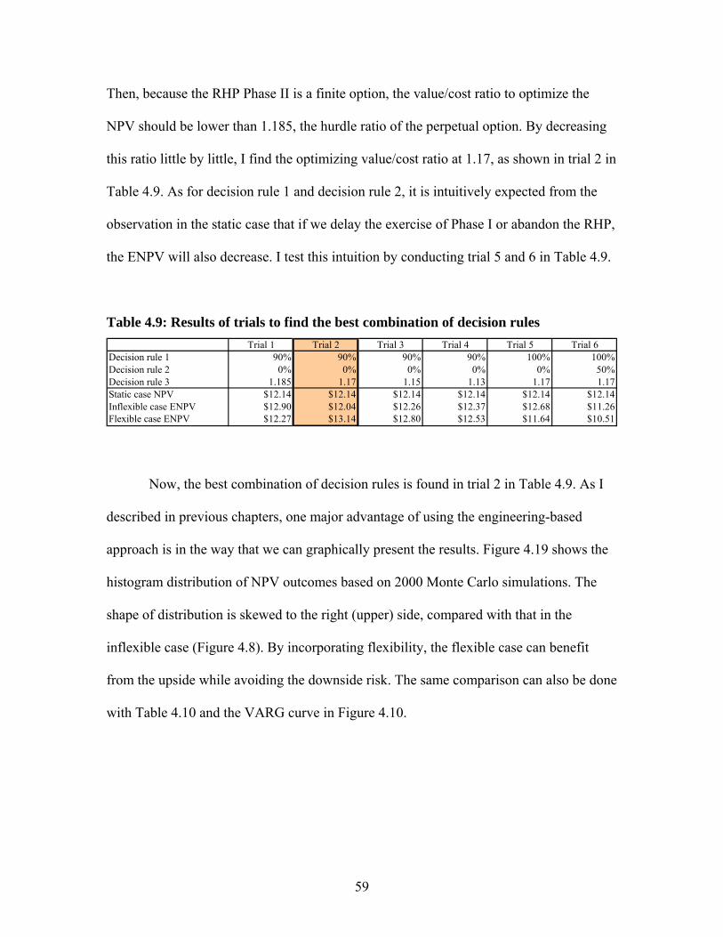
Then, because the RHP Phase II is a finite option, the value/cost ratio to optimize the

NPV should be lower than 1.185, the hurdle ratio of the perpetual option. By decreasing

this ratio little by little, I find the optimizing value/cost ratio at 1.17, as shown in trial 2 in

Table 4.9. As for decision rule 1 and decision rule 2, it is intuitively expected from the

observation in the static case that if we delay the exercise of Phase I or abandon the RHP,

the ENPV will also decrease. I test this intuition by conducting trial 5 and 6 in Table 4.9.

Table 4.9: Results of trials to find the best combination of decision rules Trial 1 Trial 2 Trial 3 Trial 4 Trial 5 Trial 6

Decision rule 1 90% 90% 90% 90% 100% 100%Decision rule 2 0% 0% 0% 0% 0%Decision rule 3 1.185 1.17 1.15 1.13 1.17 1.17Static case NPV $12.14 $12.14 $12.14 $12.14 $12.14 $12.14Inflexible case ENPV $12.90 $12.04 $12.26 $12.37 $12.68 $11.26Flexible case ENPV $12.27 $13.14 $12.80 $12.53 $11.64 $10.51

50%

Now, the best combination of decision rules is found in trial 2 in Table 4.9. As I

described in previous chapters, one major advantage of using the engineering-based

approach is in the way that we can graphically present the results. Figure 4.19 shows the

histogram distribution of NPV outcomes based on 2000 Monte Carlo simulations. The

shape of distribution is skewed to the right (upper) side, compared with that in the

inflexible case (Figure 4.8). By incorporating flexibility, the flexible case can benefit

from the upside while avoiding the downside risk. The same comparison can also be done

with Table 4.10 and the VARG curve in Figure 4.10.

59

0.0%

2.0%

4.0%

6.0%

8.0%

10.0%

12.0%

-$11.1

-$6.2

-$1.2

$3.7

$8.6

$13.5

$18.4

$23.3

$28.3

$33.2

$38.1

$43.0

$47.9

$52.9

$57.8

$62.7

$67.6

$72.5

$77.4

$82.4

$87.3

$92.2

$97.1

$102.0

$106.9

NPV ($, Millions)

Fre

qu

en

cy

Figure 4.9: Histogram distribution of NPV in the flexible case based on 2000 Monte

Carlo simulations

Table 4.10: Comparison of NPV outcomes between the inflexible case and the

flexible case Inflexible case Flexible case Better?

Expected NPV $12.04 $13.14 FlexiblePercentile (10%) -$7.86 -$2.47 FlexiblePercentile (90%) $34.06 $34.40 FlexibleMaximum NPV $88.76 $108.17 FlexibleMinimum NPV -$27.68 -$12.30 Flexible

60

0%

10%

20%

30%

40%

50%

60%

70%

80%

90%

100%

-$40.0 -$20.0 $0.0 $20.0 $40.0 $60.0 $80.0 $100.0 $120.0

NPV ($, Millions)

Cu

mu

lati

ve p

robabilit

y

VARG Flexible Case ENPV Flexible Case Static NPV

VARG Inflexible Case ENPV Inflexible Case

Figure 4.10: VARG curve based on 2000 Monte Carlo simulations

Other interesting results are shown in Table 4.11 and Figure 4.11. In trial 2 in

Table 4.9, when maximizing the ENPV based on the 2.322% monthly discount rate, the

exercise of the RHP Phase II happens only 1119 times out of 2000 simulations, as shown

in Table 4.11. This result indicates that not only the “waiting” option of the RHP Phase II,

but also its “abandonment” (i.e., not build) option can add the value of flexibility, by

reducing the probability of negative NPV. Also, Figure 4.11 depicts the timing of the

1119 times of option exercise. According to this figure, the exercise of the Phase II

option happens most likely at month 48, as soon as it becomes possible. However, the

number of this immediate exercise is about 600, less than the number of no exercise of

the option (881 times). Although this kind of analysis could also be done in the

economics-based approach, it seems to be more difficult and more complex. These

graphic presentations would work well especially when the project designer need to

61

present the result of the analysis to the managers who are not familiar with financial

theories of real options.

Table 4.11: Number of exercise of the RHP Phase I option, the RHP Phase II option,

and the abandonment option (based on trial 2 in Table 4.9)18

RHP RHP RHPPhase I Phase II Abandon

Option exercised 2000 1119 0Not exercised 0 881 2000

RHP Phase II Exercise (total 1119 out of 2000 simulations)

0

100

200

300

400

500

600

700

24 26 28 30 32 34 36 38 40 42 44 46 48 50 52 54 56 58 60

month

Freq

uenc

y

Figure 4.11: Timing of the RHP Phase II option exercise based on trial 2 in Table

4.9 (total 1119 times out of 2000 Monte Carlo simulations)

18 In Table 4.11, “RHP Abandon” means the abandonment option of RHP project. Therefore, “Not exercised” of “RHP Abandon” means that the developer exercises at least the RHP Phase I option without abandoning the RHP project. Table 4.13 is based on the same definition.

62

Summary of experiment 1

It is successfully verified that incorporating sources of flexibility can add value in

Step 4. In this case, the added value is $1.0M ($13.14M-$12.14M). Also, the

engineering-based approach showed its great ability to illustrate through useful graphic

tools such as the histogram distribution of outcome and the VARG curve. However, if we

start Step 1 of the analysis assuming that the static case NPV equals “true” real options

value, as I did here, we might overestimate the value of the land through Step 4.

Believing that the economics-based approach can always calculate the “true” options

value, I conclude that the assumption of a single risk-adjusted discount rate is not correct

in this experiment, because, as we have seen, the engineering-based model estimated the

project value at $13.14M, when the economics-based benchmark for the correct valuation

is $12.14M. (This presumes that the Step 4 flexible case ENPV is indeed the correct

metric to interpret as the project value implied by the engineering-based model. In fact,

one might ask whether the ENPV is a complete indication of what an investor should bid

for the land (or the right to develop the project), as it is only one point in a histogram of

possible NPVs, and the range or second moment in that implied ex ante probability

distribution might also have to be considered. In other words, the engineering-based

approach somewhat begs the question of the decision-maker’s “utility function,” whereas

the economics-based approach transcends this issue by basing the valuation on an

equilibrium model.)

63

4.3.2 Experiment 2

In experiment 1, the best combination of decision rules indicated that the

developer should initiate the RHP Phase I immediately and build Phase II sometime after

month 24 (or not build Phase II at all). Therefore, the timing of the exercise of the RHP

Phase I (and the abandonment option) has not affected the result.

In this experiment, I slightly modify the assumption of the case in order to

examine the effect not only of the RHP Phase II option, but also of the RHP Phase I

option and the abandonment option. What I change is only the volatility of built property

value, from 15% to 25% per annum. Based on this change, the real options value

increases to $19.07M in the economics-based approach.19 Now the immediate exercise of

the RHP Phase I is not the component of real options value. The first period where the

economics-based model indicates the immediate exercise of Phase I is month 2, with the

probability of 25.6% (out of all the probabilities in month 2).

Step 1

Here, I also assume that the developer would pay $19.07M for the land, equal to

the value calculated by the economics-based approach. Since the change in volatility of

built property value does not affect the static case cash flows, this value should still be

created by immediate exercises of the RHP Phase I and Phase II.20 As shown in Figure

19 This calculation can be easily done by just changing the volatility assumption in the model. 20 The abandonment value increases according to the increase of volatility. The abandonment value as of time zero is $7.55M, and decreases over time. Therefore, this option does not matter in obtaining the NPV of $19.14M.

64

4.12, the implied discount rate is 1.043% per month (13.26% per annum). This discount

rate is assumed in all steps in this experiment.

($, Millions)Time (month) 0 6 12 18 24 30 36 42 48Phase I Built Property Value 61.12Phase I Construction Cost 49.94Phase II Built Property Value 103.76Phase II Construction Cost 86.59Total Cash Flow 0.00 0.00 0.00 0.00 111.06 0.00 0.00 0.00 190.35

Discount Rate (monthly) 1.043%NPV 19.14

Figure 4.12: Static case pro forma summary (columns are shown semi-annually to

conserve space)

Step 2 & 3

In Step 2, I examine the effect of incorporating uncertainty in the same way as in

experiment 1. Figure 4.13 depicts the histogram distribution of NPV based on 2000

Monte Carlo simulations in the inflexible case. Compared with Figure 4.8 in experiment

1, the distribution is more widely spread, reflecting the higher volatility of built property

value. In Step 3, I use the same combinations of sources of flexibility and decision rules.

Therefore, I simply skip the discussion of Step 3 here.

65

0.0%

1.0%

2.0%

3.0%

4.0%

5.0%

6.0%

7.0%

8.0%

9.0%

10.0%

-$59.0

-$42.0

-$25.0

-$8.1

$8.9

$25.9

$42.9

$59.9

$76.8

$93.8

$110.8

$127.8

$144.8

$161.7

$178.7

$195.7

$212.7

$229.6

$246.6

$263.6

$280.6

$297.6

$314.5

$331.5

$348.5

NPV ($, Millions)

Fre

qu

en

cy

Figure 4.13: Histogram distribution of the project NPV in the inflexible case based

on 2000 Monte Carlo simulations

Step 4

In this step, I have to use more complex procedure to find the best combination of

decision rules than I did in experiment 1, because not only the RHP Phase II option but

also the Phase I option and the abandonment option affect the results in this experiment.

First, I fix decision rule 1 and decision rule 2 in order to always assume the

immediate exercise of the RHP Phase I in the same way as I did in experiment 1. The

currently expected exercise profit of the RHP Phase I is still $5.27M, but the

abandonment value as of now increases to $7.55M due to higher volatility. Therefore, I

set decision rule 1 to 69%. Next, I use the Samuelson-McKean formula to set the

benchmark of the level of decision rule 3. Using again equation (9) from Chapter 3, the

hurdle value/cost ratio for a perpetual option is given by the followings:

66

487.1)105.3(

05.3)1(

*

0

=−

=−

=ηη

KV

Then, in the same way as in experiment 1, I decrease the above ratio little by little, and I

find the optimizing value/cost ratio at 1.40, as shown in trial 2 in Table 4.12. The ENPV

is $25.11M, $5.97M above the static case NPV.

Next, I change only decision rule 1 and examine the effect of “delaying” the

construction of the RHP Phase I, keeping constant the level of decision rule 2 (no

abandon) and decision rule 3 (1.40). By increasing the level of decision rule 1, I find the

optimizing level of 75% at trial 4 in Table 4.12. By incorporating the flexibility of

delaying the construction of the RHP Phase I, the ENPV of the flexible case increases to

$26.09M.21

Finally, I examine the effect of varying decision rule 2, the abandonment option.

As is shown in trial 6 in Table 4.12, incorporating the flexibility of abandonment does not

add the ENPV. As is examined in Table 4.13 and Figure 4.14, the abandonment of the

RHP project happens 684 times out of 2000 Monte Carlo simulations in trial 6, and

almost all the abandonment happens within the first 12 months. Even though I set

decision rule 2 so that the developer will abandon the RHP project only when the

expected profit of Phase I project goes below 10% of the abandonment value, one-third

of simulated scenarios show abandonment results. This is probably because the expected

profit of the RHP Phase I could go below 0 with certain probability. The result of trial 6

shows that intermediate abandonment of the RHP project between month 0 and 35 does

21 It should be noted that even though I assume no abandonment from trial 1 to trial 6 in Table 4.12, there will be abandonment only at month 36, when the scenario does not achieve the decision rule 1 (the RHP Phase I exercise) at any time between month 0 and 36.

67

not add the value of flexibility. No matter how low the expected profit of Phase I might

be, it is better not to abandon and to simply hold the option lived until month 36.

Table 4.12: Result of trials to find the best combination of decision rules Trial 1 Trial 2 Trial 3 Trial 4 Trial 5 Trial 6

Decision rule 1 69% 69% 69% 75% 80% 75%Decision rule 2 0% 0% 0% 0% 0%Decision rule 3 1.49 1.40 1.30 1.40 1.40 1.40Static case NPV $19.14 $19.14 $19.14 19.14 $19.14 $19.14Inflexible case ENPV $18.84 $19.84 $20.02 19.20 $19.50 $18.17Flexible case ENPV $24.03 $25.11 $24.93 26.09 $24.91 $21.47

10%

Table 4.13: Number of exercise of the RHP Phase I option, the RHP Phase II option,

and the abandonment option (based on trial 6 in Table 4.12) RHP RHP RHP

Phase I Phase II AbandonOption exercised 1316 645 684Not exercised 684 1355 1316

RHP Abandon (total 684 out of 2000 simulations)

0

50

100

150

200

250

0 2 4 6 8 10 12 14 16 18 20 22 24 26 28 30 32 34 36

month

Freq

uenc

y

Figure 4.14: Timing of the RHP project abandonment based on trial 6 in Table 4.12

(total 684 times out of 2000 Monte Carlo simulations)

68

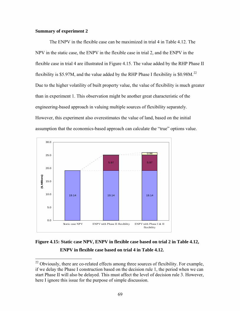
Summary of experiment 2

The ENPV in the flexible case can be maximized in trial 4 in Table 4.12. The

NPV in the static case, the ENPV in the flexible case in trial 2, and the ENPV in the

flexible case in trial 4 are illustrated in Figure 4.15. The value added by the RHP Phase II

flexibility is $5.97M, and the value added by the RHP Phase I flexibility is $0.98M.22

Due to the higher volatility of built property value, the value of flexibility is much greater

than in experiment 1. This observation might be another great characteristic of the

engineering-based approach in valuing multiple sources of flexibility separately.

However, this experiment also overestimates the value of land, based on the initial

assumption that the economics-based approach can calculate the “true” options value.

19.14 19.14 19.14

5.97 5.97

0.98

0.0

5.0

10.0

15.0

20.0

25.0

30.0

Static case NPV ENPV with Phase II flexibility ENPV with Phase I & IIflexibility

($, M

illio

ns)

Figure 4.15: Static case NPV, ENPV in flexible case based on trial 2 in Table 4.12,

ENPV in flexible case based on trial 4 in Table 4.12.

22 Obviously, there are co-related effects among three sources of flexibility. For example, if we delay the Phase I construction based on the decision rule 1, the period when we can start Phase II will also be delayed. This must affect the level of decision rule 3. However, here I ignore this issue for the purpose of simple discussion.

69

4.3 Findings of case study

In both experiments, I arbitrarily assumed a single constant risk-adjusted discount

rate, as derived in Step 1. However, as I described in the economics-based approach

(Table 4.6), the (implied) discount rate varies over time in the project with uncertainty. In

this particular case, the discount rate decreases as the option’s expiration approaches.

Moreover, the (implied) discount rate varies at each node of the binominal trees, even

within the same period of time. Therefore, using a single constant discount rate is not

well suited in calculating the exact value of flexibility.

Regarding this issue, Hodder, Mello, and Sick (2001) demonstrated that a single

risk-adjusted discount rate is inconsistent with option valuation, and introduced a way to

use the varying risk-adjusted discount rate at each node of the binominal option valuation

model. The authors examined the method of using the Capital Asset Pricing Model

(CAPM) to determine the risk-adjusted discount rate for each node of the binominal tree.

Although they clarified that this method can calculate the options value correctly, the

procedure of calculating all discount rates is cumbersome and less efficient than the

widely used risk-neutral approach. The authors concluded that even though multiple risk-

adjusted discount rates work well for option valuation, the simplest valuation method for

valuing real options would be the risk-neutral approach.

In principle, it is also possible for the engineering-based approach to obtain the

approximate correct value of flexibility by correctly using the risk-neutral dynamics.

However, as previously mentioned, since the main focus of this thesis is to examine the

simplicity and the transparency of the engineering-based approach, and to make it easy

70

for average practitioners to recognize the value of flexibility, I do not introduce the risk-

neutral dynamics here into the engineering-based approach.

71

Chapter 5 Conclusion

The goal of this thesis was to compare the engineering-based real options

approach with the economics-based approach. I reviewed the types of real options as well

as the types of option valuation methods in Chapter 2. Then the methodologies of both

approaches were set up in Chapter 3 in order to conduct a fair comparison.

In Chapter 4, I compared the results of both option valuation approaches, using a

real estate development case study. Through the two experiments in the case study, the

engineering-based approach showed its great capability to present the results graphically

in many ways. Not only the project designer who uses the model but also the senior

manager who will make the final decision in the firm will be able to easily understand the

procedure of this approach. However, the land price calculated by the engineering-based

approach was overestimated in the two experiments. This result is mainly due to the

arbitrary assumption that the static case of the engineering-based approach starts from the

“true” land price, which is calculated in the economics-based approach. In other words,

depending on the initial assumption of the single risk-adjusted discount rate in the static

case, the result of the flexible case could either overvalue or undervalue the land price.

The problem of using a single risk-adjusted discount rate was pointed out through

the case study. In many projects incorporating uncertainty as well as flexibility, the risk

and return characteristics are changing with the time to option’s maturity and the value of

the underlying asset. Therefore, a single risk-adjusted discount rate is not appropriate in

calculating the value of flexibility. By using varying discount rates or the risk-neutral

dynamics, this problem could be alleviated. However, this modification would make the

72

model too complicated and spoil the simplicity and the transparency of the engineering-

based approach.

Table 5.1 summarizes the merits and the demerits of both approaches discussed in

this thesis. Recognizing these merits and demerits, I propose to use the engineering-based

approach together with the economics-based approach for a more accurate decision-

making process. Even though the senior decision-maker in the firm might not be able to

understand the advanced financial theory, the project designer could explain his analysis

based on the engineering-based approach with a lot of useful graphic tools, while

ensuring that the result of the engineering-based approach is consistent with the rigorous,

economics-based approach. If used together with the economics-based approach, the

engineering-based approach will be able to bring its great ability of valuing flexibility

into the real world.

Table 5.1: Merits and demerits of the economics-based approach and the

engineering-based approach

Economics-based approach Engineering-based approach

Merits

・ It can calculate the "true" realoptionsprice under the marketequibrium theory.

・

・

・

The user does not need to understandadvanced financial theory.The analysis can be done withnormal computational resources.It has many ways to present theresult graphically.

Demerits・ The user needs to understand the

financial theory of real options.

・ It is not always possible to calculate"true" real options value, mainly dueto the arbitrary assumption of singlerisk-adjusted discount rate.

73

Bibliography

Amram, M., & Kulatilaka, N. (1999), Real Options: Managing Strategic Investment in an

Uncertain World, Harvard Business School Press, Boston, MA.

Ariizumi, T. (2006), “Evaluation of Large Scale Industrial Development Using Real

Options Analysis: A Case Study,” Master’s Thesis, Department of Architecture,

Massachusetts Institute of technology, Cambridge, MA.

Arnold, T., & Crack, T. (2003), “Option Pricing in the Real World: A Generalized

Binominal Model with Applications to Real Options,” Department of Finance, University

of Richmond, Working Paper

Barman, B., & Nash, K. (2007), “A Streamlined Real Options Model for Real Estate

Development,” Master’s Thesis, Department of Urban Studies and Planning,

Massachusetts Institute of technology, Cambridge, MA.

Bodie, Z., Kane, A., & Marcus A. J. (2005), Investments, 6th ed., McGraw-Hill, New

York, NY.

Brealey, R. A., Myers, S. C., & Allen, F. (2006), Principles of Corporate Finance, 8th ed.,

McGraw-Hill, New York, NY

Cardin, M-A. (2007), “Facing Reality: Design and Management of Flexible Engineering

Systems,” Master’s Thesis, the Engineering Systems Division, Massachusetts Institute of

technology, Cambridge, MA.

Copeland, T., & Antikarov, V. (2003), Real Options: A Practitioner’s Guide, Texere,

New York, NY.

Cox, J.C., Ross, S.A., & Rubinstein, M. (1979), “Option Pricing: A Simplified

Approach,” Journal of Financial Economics, 7, pp. 229-263

74

de Neufville, R., Scholtes, S., & Wang, T. (2006), “Real Options by Spreadsheet: Parking

Garage Case Example,” Journal of Infrastructure Systems, 12 (2), pp. 107-111.

de Neufville, R. (2005), “Lecture Notes,” ESD.71, Engineering Systems Division,

Massachusetts Institute of Technology, Cambridge, MA

DiPasquale, D. & Wheaton, W. C. (1996), Urban Economics and Real Estate Markets,

Prentice Hall, Englewood Cliffs, NJ

Dixit, A. K., & Pindyck, R.S. (1994), Investment Under Uncertainty, Princeton

University Press, Princeton, NJ.

Geltner, D., Miller N., Clayton, J., & Eichholtz, P. (2007), Commercial Real Estate

Analysis & Investments, 2nd ed., Thomson South-Western, Mason, OH.

Geltner, D., Riddiough, T. & Stojanovic, S. (1996), “Insights on the Effect of Land Use

Choice: The Perpetual Option on the Best of Two Underlying Assets,” Journal of Urban

Economics, no.39, pp. 20-50.

Hengels, A. (2005), “Creating a Practical Model Using Real Options to Evaluate Large-

Scale Real Estate Development Projects,” Master’s Thesis, Department of Architecture,

Massachusetts Institute of technology, Cambridge, MA.

Hodder, J., Mello, A., & Sick, G. (2001), “Valuing Real Options: Can Risk-Adjusted

Discounting Be Made to Work?,” Journal of Corporate Finance, 14 (2), pp. 90-101.

Hull, J. (2006), Options, Futures, and Other Derivatives, 6th ed., Prentice Hall,

Englewood Cliffs, NJ

Imai, J. (2004), Real Options: Engineering Approach to Investment Valuation, Chuo-

Keizai-Sha, Tokyo

75

Kang, J. (2004), “Valuing Flexibilities in Large-Scale Real Estate Development

Projects,” Master’s Thesis, Department of Urban Studies and Planning, Massachusetts

Institute of technology, Cambridge, MA.

McDonald, R. (2006), “The Role of Real Options in Capital Budgeting: Theory and

Practice,” Journal of Applied Corporate Finance, 18 (2), pp. 28-39.

Mun, J. (2006), Real Options Analysis: Tools and Techniques for Valuing Strategic

Investments and Decisions, 2nd ed., John Wiley & Sons, Hoboken, NJ

Myers, S. C. (1984), “Finance Theory and Financial Strategy,” Interfaces, 14(1), January-

February, pp.126-137

Sheen, V. (2004), “Real Options Theory and the Pricing of Residential Land-Use Rights

in Shanghai,” Master’s Thesis, Department of Urban Studies and Planning,

Massachusetts Institute of technology, Cambridge, MA.

Trigeorgis, L. (1996), Real Options: Managerial Flexibility and Strategy in Resource

Allocation, MIT Press, Cambridge, MA.

Yoshida, J. (1999), “Effects of Uncertainty on the Investment Decision: An Examination

of the Option-Based Investment Model Using Japanese Real Estate Data,” Master’s

Thesis, Department of Urban Studies and Planning, Massachusetts Institute of technology,

Cambridge, MA.

76