A Comparative Study of Moored/Point and Acoustic Tomography/IntegralObservations of Sound Speed in Fram Strait Using Objective

Mapping Techniques

BRIAN D. DUSHAW AND HANNE SAGEN

Nansen Environmental and Remote Sensing Center, Bergen, Norway

(Manuscript received 17 December 2015, in final form 5 July 2016)

ABSTRACT

Estimationof theexchangeof seawaterofvariouspropertiesbetween theArctic andNorthAtlanticOceanspresentsa

challenging observational problem. The strong current systems within Fram Strait induce recirculations and a turbulent

ocean environment dominated by mesoscale variations of 4–10-km scale. By employing a simple parameterized model

formesoscalevariabilitywithinFramStrait, theauthors examine theabilityof a linearrayof closely spacedmoorings and

an acoustic tomography line to measure the average sound speed, a proxy variable for ocean temperature or heat

content. Objective maps are employed to quantify the uncertainties resulting from the different measurement ap-

proaches.Whilemeasurements by amooring line and tomography result in similar uncertainties in estimations of range-

and depth-averaged sound speed, the combination of the two approaches gives uncertainties 3 times smaller. The two

measurements are sufficiently different as to be complementary; onemeasurement provides resolution for the aspects of

the temperature section that the other misses. The parameterized model and its assumptions as to the magnitudes and

scales of variabilitywere tested by application to a hydrographic section across FramStrait measured in 2011. This study

supports the deployment of the 2013–16 Arctic Ocean under Melting Ice (UNDER-ICE) network of tomographic

transceivers spanning the ongoingmoored array line across Fram Strait. Optimal estimation for this ocean environment

may require combining disparate data types as constraints on a numerical ocean model using data assimilation.

1. Introduction

Fram Strait, the passage between Spitsbergen and

Greenland, is a significant ‘‘choke point’’ for the general

circulation of the world’s oceans (Fieg et al. 2010;

Schauer et al. 2008). This strait is the only deep con-

nection between the Arctic and the world’s oceans.

Through this strait, warm, salty North Atlantic water

flows northward in the West Spitzbergen Current, while

cold, fresher water, together with considerable quanti-

ties of ice (Smedsrud et al. 2011), flows southward in the

East Greenland Current. The transports of heat and salt

between the Atlantic basin and the Arctic Basin by the

deep and shallow current systems in Fram Strait are

important aspects of ocean circulation, with profound

impacts on the ocean’s climate.

The details of these current systems are, however,

difficult to observe. Not only are the natural scales of

variability small at these high latitudes but the powerful

current systems have turbulent and recirculating fea-

tures. These features influence and obscure transports of

mass or heat. Eddy variability may be an important

contributor to these transports. The Fram Strait moored

array (Fig. 1) has been deployed across the strait since

1997 to measure the properties of these current systems

(Fieg et al. 2010; Schauer et al. 2008). Temperature,

salinity, and current data from this array have been

noted for their great variability (von Appen et al. 2015).

Even with 16 moorings deployed along a 325-km line

across the strait, however, the separation of the moor-

ings (20–28 km) is a few times larger than the natural

scales of variability, 4–10 km (Fieg et al. 2010; Nurser

and Bacon 2014). The moored array has therefore un-

dersampled the ocean variability; the Fram Strait

moored array forms an incoherent observing array. This

situation has made it challenging to employ the moored

Corresponding author address: Brian D. Dushaw, Nansen En-

vironmental and Remote Sensing Center, Thormøhlens Gate 47,

N-5006 Bergen, Norway.

E-mail: brian.dushaw@nersc.no

Denotes Open Access content.

OCTOBER 2016 DUSHAW AND SAGEN 2079

DOI: 10.1175/JTECH-D-15-0251.1

� 2016 American Meteorological SocietyUnauthenticated | Downloaded 04/03/22 05:18 PM UTC

array data directly to estimate heat flow (Schauer et al.

2008; Schauer and Beszczynska-Möller 2009), or as

constraints on numerical ocean models through data

assimilation. The high noise of the observations

overwhelms the signals of interest to the ocean

modelers and introduces the effects of aliasing. Other

observing approaches, such as glider or conductivity–

temperature–depth (CTD) sections, have obvious,

different sets of complications or deficiencies. It is

clear that no one type of measurement offers a com-

prehensive solution to the observation problem in

Fram Strait.

Ocean acoustic tomography offers a natural in-

tegrating measurement type for sound speed that is

complementary to the point (moored or CTD) data type

(Munk et al. 1995). The technique has been previously

explored as a way to measure temperature or currents in

Fram Strait using realistic simulations (Chiu et al. 1987;

Naugolnykh et al. 1998). Tomography offers a natural

integral measurement of large-scale temperature. If one

of the aims of the Fram Strait observations is an accurate

estimate of the transport of net heat through the strait,

then large-scale temperature may be one relevant pa-

rameter. For these reasons, the Nansen Environmental

and Remote Sensing Center (NERSC) in Bergen, Nor-

way, developed the Developing Arctic Modeling and

Observing Capabilities for Long-Term Environmental

Studies (DAMOCLES) tomography experiment as a

pilot study. The study included the deployment of a

single tomographic path of about 130-km range during

2008–09 (Skarsoulis et al. 2010; Mikhalevsky et al. 2015)

(Fig. 1). Tomographic observations were subsequently

expanded with the 2009–11 Acoustic Technology for

Observing the Interior of the Arctic Ocean (ACOBAR)

deployments (Fig. 1), and they were sustained with the

Arctic Ocean under Melting Ice (UNDER-ICE) program

with observations spanning 2013–16. Not surprisingly, the

nature of the data from the actual measurements is con-

siderably different than those employed in the previous

simulation studies (Dushaw et al. 2016b).

In addressing the measurement problem by employing

basic objective mapping techniques, this paper has three

main aims. The first aim is to describe the different

measurement properties of the moored array and to-

mography. The difference in these properties illustrates

the mutual advantage of employing both data types in an

observation system. The second aim is to document the

inverse of the tomography data to obtain an estimate

for ocean temperature. This approach was used by

Sagen et al. (2016) to estimate temperature from the

DAMOCLES tomography data. The third aim is to use

the analysis as a first step toward assimilation of the to-

mography data type to constrain numerical ocean

models. The results of this analysis are intended to build

intuition as to the nature of the information content of the

tomography data; these results suggest how a numerical

ocean model might respond to the constraints of this in-

formation. In this paper it is important to distinguish

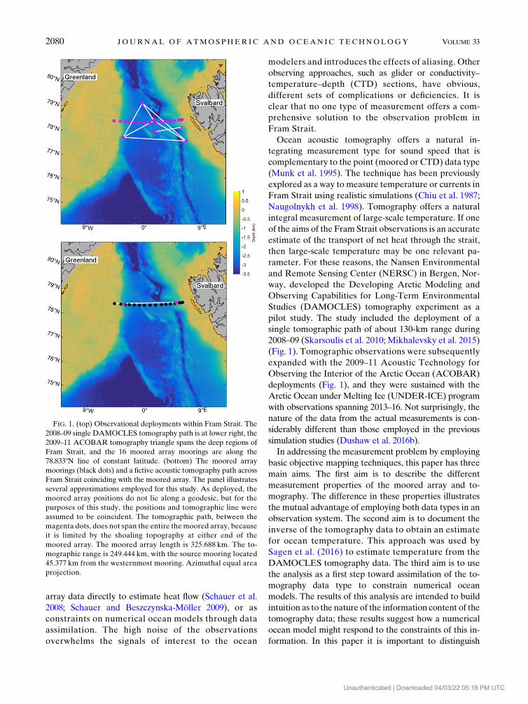
FIG. 1. (top) Observational deployments within Fram Strait. The

2008–09 single DAMOCLES tomography path is at lower right, the

2009–11 ACOBAR tomography triangle spans the deep regions of

Fram Strait, and the 16 moored array moorings are along the

78.8338N line of constant latitude. (bottom) The moored array

moorings (black dots) and a fictive acoustic tomography path across

Fram Strait coinciding with the moored array. The panel illustrates

several approximations employed for this study. As deployed, the

moored array positions do not lie along a geodesic, but for the

purposes of this study, the positions and tomographic line were

assumed to be coincident. The tomographic path, between the

magenta dots, does not span the entire the moored array, because

it is limited by the shoaling topography at either end of the

moored array. The moored array length is 325.688 km. The to-

mographic range is 249.444 km, with the source mooring located

45.377 km from the westernmost mooring. Azimuthal equal area

projection.

2080 JOURNAL OF ATMOSPHER IC AND OCEAN IC TECHNOLOGY VOLUME 33

Unauthenticated | Downloaded 04/03/22 05:18 PM UTC

between a simple ocean model of an objective map,

consisting of a parameterization employing small sets of

vertical and horizontal basis functions, and a complex

numerical ocean model, consisting of atmospheric forc-

ing, ocean dynamics, etc., and a gridded scheme for

computing the temporal evolution of the ocean state. This

paper is an application of the former but with an eye on

the latter.

As shown by Dushaw et al. (2016b) and Sagen et al.

(2016), the non-bottom-interacting acoustic propaga-

tion associated with the DAMOCLES measurements

was mainly confined to the upper half of the water

column. In addition, as shown by Dushaw et al.

(2016a), sound speed is an accurate proxy variable to

temperature to good approximation, except, perhaps,

in near-surface conditions. Although salinity is obvi-

ously an important quantity governing and marking

oceanographic variability, its influences on the acous-

tic propagation and analysis here can be neglected.

The acoustic data therefore represent a measure of

ocean temperature that inherently averages over the

upper part of the water column. Given the nature of this

measurement, the average sound speed over the upper

1000m of ocean and over the range of acoustic propa-

gation was employed here. This average is closely aligned

with the acoustic measurements, and it is a convenient

single parameter for comparing the different data types.

Sound speed was used as a parameter of convenience

here, since this was the quantity directly measured by the

acoustics. As noted, this parameter can be used to com-

pute temperature, hence heat content.

Objective maps (inverse and weighted least squares

are equivalent terms and used interchangably) are a

way to combine different data types in a consistent way

(Cornuelle et al. 1989, 1993). These techniques were

employed by Dushaw et al. (1993a,b) for combining

XBT/CTD and tomographic data types to test the

equations of sound speed and to estimate heat content

alongO(1000) km sections in the eastern North Pacific.

Morawitz et al. (1996a) used similar inverse methods to

combine hydrographic, acoustic, and moored thermis-

tor data to obtain optimal estimates for the three-

dimensional temperature field of deep convection in

the Greenland Sea (although the Greenland Sea is only

about 300 km south of Fram Strait, it has very different

oceanographic conditions). Skarsoulis et al. (2010)

have previously estimated temperature variability from

DAMOCLES tomography data. They first computed

two-dimensional (2D) empirical orthogonal functions

(EOFs) from the moored array data, and then esti-

mated the amplitudes of those EOFs. The EOF am-

plitudes were estimated by a brute-force search for

EOF combinations that gave acoustic predictions that

matched the observations. The objective map approach

discussed here is a more versatile and less computa-

tionally intensive approach to an inverse. Objective

maps require the design of a parameterized ocean

model for an infinite number of possible ocean states

are consistent with known ocean properties. The aim

of the objective map is to determine the solution

from this infinite pool of possible solutions that best

fits the data, within the assumed constraints of as-

sociated model variances and data noise. With any

objective mapping approach, the results are de-

pendent on the assumed model employed for the

study. This paper therefore begins with a brief dis-

cussion of possible ocean models that might capture

the Fram Strait oceanography. Within the limitations

of a parameterization of the ocean by a simplistic

ocean model (a ‘‘toy’’ model), the study will quan-

titatively illustrate the value of the integrating, to-

mographic data type in estimating heat content

averaged across Fram Strait.

2. The ocean model: Vertical EOFs, sines andcosines, and statistical properties

The natural or obvious approach to assessing the

information content of various data types within Fram

Strait would be to follow the approach of Cornuelle

et al. (1989) and Morawitz et al. (1996a), and compute

three-dimensional inverse estimates for ocean tem-

perature. Such an approach might be amenable to

observations as depicted in the top panel of Fig. 1. It

would not directly elucidate the relative contributions

of the data types, however, since the various observa-

tions are displaced from one another. Further, such an

approach would require the construction of a three-

dimensional ocean model for Fram Strait, which would

quickly become a challenging endeavor. One would

have to account for mean flows, eddy meanders, re-

circulation characteristics, etc. For these reasons, the

approach here is artificially reduced to two dimensions,

with the moored array positions adjusted to lie on a

geodesic path coincident with a fictive tomography path

(Fig. 1, bottom panel). In two dimensions, a simpler sta-

tistical ocean model can be employed to determine the

basic resolution characteristics of the data types.

An objective map begins with a suitable reference

ocean in which data that are equivalent to the mea-

surements can be computed (Munk et al. 1995;

Cornuelle et al. 1989, 1993; Morawitz et al. 1996a).

‘‘Suitable’’ means the differences between computed

and measured data are small such that the ensuing in-

verse can be considered linear. Using the differences

between the reference-ocean data and measurements,

OCTOBER 2016 DUSHAW AND SAGEN 2081

Unauthenticated | Downloaded 04/03/22 05:18 PM UTC

the objective map obtains a correction to the reference

ocean, forming an estimate for the true ocean. For this

study, the reference ocean employed was the World

Ocean Atlas 2009 (Antonov et al. 2010; Locarnini et al.

2010). The climatological mean of the ocean across the

Fram Strait is shown by sections of temperature, salinity,

and sound speed along the moored array section (Fig. 2).

The core of the West Spitzbergen Current is apparent

over the continental slope west of Spitzbergen, extending

to about 500-m depth. The mesoscale variability domi-

nates the climatological mean, however.

Considerable oceanographic knowledge is required

to devise an ocean model that accurately captures the

expected ocean variability. The formulation of this

model is the main oceanographic problem for objec-

tive mapping (indeed, present knowledge of the

three-dimensional variability within Fram Strait

may not be sufficient to construct a reliable three-

dimensional model). The model is a set of functions of

depth and range that accurately depicts the expected

variability, together with associated statistical de-

scriptions of the covariances in depth and range. The

statistics were assumed to be Gaussian throughout,

and the inverse (i.e., the solution for the ocean state

by a weighted least squares fit of the model to the

data) is assumed to be linear. The assumptions about

model functions, statistics, and linearity may not be

entirely accurate. Nevertheless, short of egregious

errors in these elements, the objective map approach

will produce a reasonable, best possible estimate of

the ocean state and its uncertainty. The objective map

approach therefore is an important component of any

rigorous design study for ocean observing.

For the ocean model in this study, we assumed the

horizontal and vertical variability were separable; that

is, if F(r, z) is the ocean state of a scalar variable, such as

sound speed or temperature, to be estimated, then it can

be modeled as a linear superposition of 2D functions of

range r and depth z,

F(r, z)5 �N

n51

AnPn(r, z)5 �

NV

i51�NH

j51

AijV

i(z)H

j(r) , (1)

where the sums are over the vertical (i) and horizontal

( j) indexes. The amplitude associated with the ith ver-

tical function and jth horizontal function is denoted

byAij. It is certainly possible to avoid this assumption by

devising sets of 2D functions that might accurately

model the ocean. Such functions might be 2D EOFs, for

example, derived from estimates of the 2D covariance of

the ocean (Skarsoulis et al. 2010). The separability

assumption simplifies matters considerably without ad-

versely affecting the ocean model estimates.

The horizontal variability was assumed to be

composed of the linear superposition of sinusoids,

sin(Kjr) and cos(Kjr); that is, the horizontal vari-

ability was modeled using a truncated Fourier series.

While more sophisticated horizontal functions are

certainly possible—for example, horizontal modes

tuned to describe the horizontal variations of the

West Spitzbergen Current—sines and cosines can

accurately account for horizontal variability in most

situations (a truncated Fourier series may not be

an appropriate model for sharp ocean fronts). The

wavenumbers are Kj 5 2pj/1:5L, where L is the range of

the Fram Strait section. In defining the wavenumbers, this

FIG. 2. World Ocean Atlas hydrographic parameters along the

moored array section, extending onto theWest Spitzbergen shelf to the

right and into the East Greenland Current to the left. The acoustic

section used for this study was between the two magenta lines. The

bathymetric data are derived from the InternationalBathymetricChart

of the Arctic Ocean (IBCAO) 2-min-resolution database (Jakobsson

et al. 2008). (top) Temperature, (middle) salinity, and (bottom) sound

speed. Note the shallow layer of the low-salinity water of the East

Greenland Current across the section, deepening to the west.

2082 JOURNAL OF ATMOSPHER IC AND OCEAN IC TECHNOLOGY VOLUME 33

Unauthenticated | Downloaded 04/03/22 05:18 PM UTC

length is increased by a factor of 1.5 to avoid the periodicity

effects at the ends of the section (Morawitz et al. 1996a). If

there are NV vertical functions and NH wavenumbers,

then a total of N5NV(2NH 1 1) 2D functions comprise

theoceanmodel.With themodel employedhere,NV was 5,

while NH was 50, giving a total of 505 2D functions.

The wavenumber spectrum assumed for the sinusoids

determines the spatial length scales associated with the

model. This spectrum defines the weights or variances

associated with each wavenumber.While its form can be

prescribed in any number of ways to best model ocean

variability, the form for the wavenumber spectrum

employed here (Fig. 3) was

Sij5

wi

Xi

1

K2j 1K2

0i

, (2)

where indexes i and j refer to vertical and horizontal

function indexes, respectively; Xi is the horizontal scale

of the ith vertical function; and K0i 5 2p/Xi. The wi de-

note scale factors, which are described below. The

Lorentzian form of this spectrum is derived from the

assumption that the spatial covariance has an expo-

nential falloff with range; the Fourier transform of a

decaying exponential is a Lorentzian. The effect of in-

cluding ‘‘K20i’’ in the denominator is to cause the spec-

trum near-zero wavenumber to roll over to a modest

finite value rather than become infinite. The Xi are

tuned to select the typical length scales desired for the

ocean model, typically 10 to a few hundred kilometers.

The spectrum used for the objective maps had

X1 5 200 km, X2 5 100 km, X3 5 50km, X4 5 30km, . . .;

higher-order modes correspond to shorter length scales

(the Xi are wavelengths associated with the truncated

Fourier series; scales of variability are smaller than these

wavelengths). The overall level for the spectrum is

scaled by wi so that it is consistent with vertical function

variances, as described next.

The vertical functions employed in an objective

map require careful consideration. Information on the

nature of the variability in the vertical in Fram Strait

was determined from a variety of sources, including

the moored array data, glider data, CTD data (see

section 6), and the results of a regional high-resolution

numerical ocean model (HYCOM) for Fram Strait

computed by the Nansen Environmental and Remote

Sensing Center modeling group (Sagen et al. 2016).

No single parameterized model could encompass all

of the variances, length scales, and other properties

suggested by these sources. The ultimate vertical pa-

rameterization was obtained by approximating the

variance as a function of depth and vertical correla-

tion length to be similar to Fram Strait variability. In

particular, the variances as a function of depth as-

sumed for this study are similar to those observed by

the moored array (Dushaw et al. 2016b). There are

many possibilities for the vertical functions, such as

baroclinic modes, layers, or the direct value at par-

ticular depths. In cases where acoustics are employed,

FIG. 3. Three possible wavenumber spectra for the first three

vertical EOFs: (top) a model for an ocean with very short length

scales (all wavenumbers have similar variance); (middle) themodel

assumed for this study, with reasonable length scales approximat-

ing those in Fram Strait; (bottom) a model with very long length

scales (only small wavenumbers have significant variance). The

middle panel was deemed the reasonable spectrum (see text). The

top panel used values 10 times these lengths, while the bottom

panel used values 0.1 times these lengths. The first EOF has the

largest variance, the third EOF the smallest.

OCTOBER 2016 DUSHAW AND SAGEN 2083

Unauthenticated | Downloaded 04/03/22 05:18 PM UTC

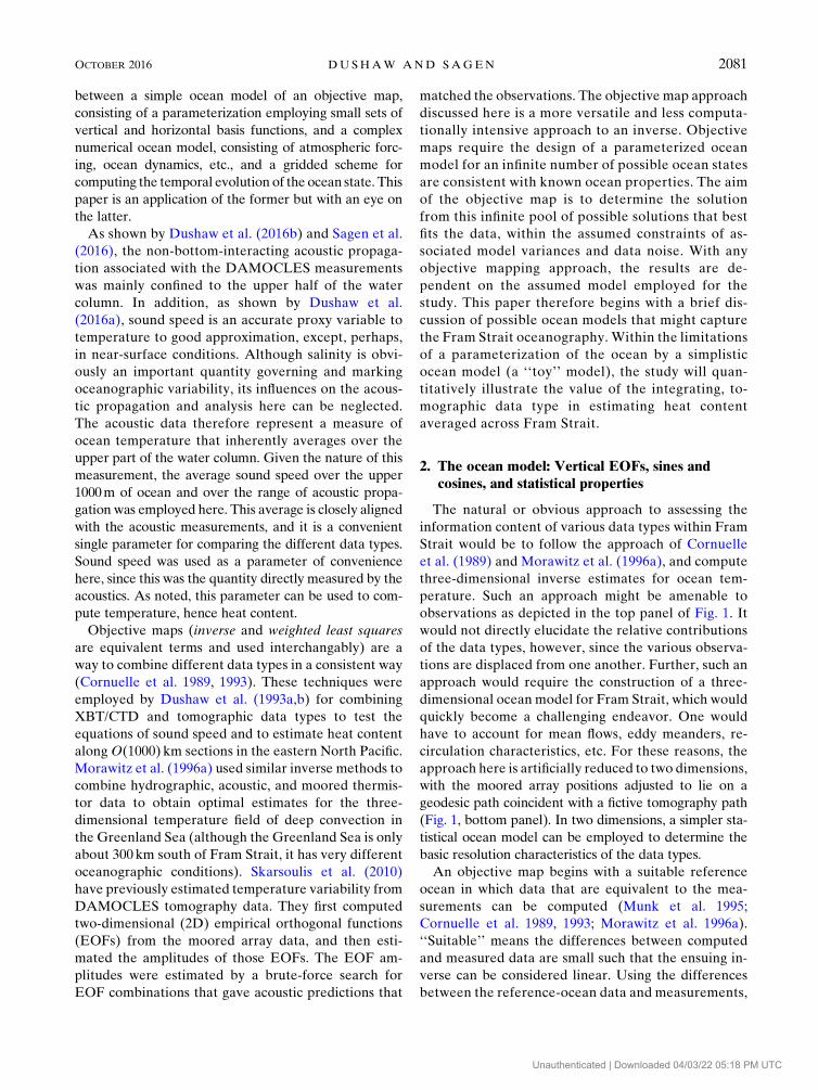
it is important to model vertical variability such that

large sound speed gradients are avoided, unless there

are compelling reasons to include such gradients, for

example, a known mixed layer. Sound propagation is

sensitive to sound speed gradients. Ocean state esti-

mates with unphysically large gradients as a conse-

quence of insufficient ocean data can cause unphysical

acoustic propagation (Dushaw et al. 2013). EOFs for

the vertical variability derived from either data or

numerical ocean models are smoothly varying func-

tions that work well for acoustics. The vertical func-

tions employed for this study were EOFs of a synthetic

covariance function (see Morawitz et al. 1996a). If

sz5 z1 1 z2 and dz5 z1 2 z2, then the (symmetric)

synthetic covariance was given by

C(z1, z

2)5 20e2sz/750e2dz2/100sz . (3)

In this model, the variance of sound speed at the sur-

face was assumed to be about 20 (m s21)2, and the

e-folding scale of variance with depth is 350m (Fig. 4).

This covariance was subsequently adjusted near the

surface, however. The variances within 40m of the

surface were increased in an ad hoc fashion to model

the ubiquitous near-surface mixed layer found in Fram

Strait. This increase is evident in the variance near the

surface in the left panel of Fig. 4. The singular value

decomposition of this covariance gives the EOFs that

model the vertical variability (Fig. 4) and the associ-

ated spectrum of these functions, fEig (Fig. 5). The

fEig specify the variance of each EOF to be used for

the objective map.

The two-dimensional functions used to model the sec-

tion across Fram Strait are combinations of vertical EOFs

and horizontal sinusoids. The variance of each EOF is

apportioned to the horizontal functions according to the

assumed wavenumber spectrum. By Parseval’s theorem,

an EOF variance specifies the value of the sum of

wavenumber variances. In the assumed model, all ver-

tical EOFs have the same shape of the wavenumber

spectra. In short, the scale factors wi are determined by

the requirement that

Ei5

wi

Xi

�NH

j51

1

K2j 1K2

0i

. (4)

The ocean model described above is

F(r,z)5�NV

i51

Vi(z)

(A0

i01�NH

j51

[A1ij cos(Kj

r)1A2ij sin(Kj

r)]

);

(5)

hence, the 2D functions have the form

Pn(r, z)5V

i(z), V

i(z) cos(K

jr), or V

i(z) sin(K

jr)

(6)

with an amplitude that is one of fA0i0, A

1ij, A

2ijg for the

mean, cosine, or sine functions.

Using the variances of the amplitudes, Sij, it is straight-

forward to derive statistically consistent snapshots of what

the ocean looks like under the model assumptions. Any

particular snapshot can be derived using amplitudes for

the 2D functions given by

An5

ffiffiffiffiffiffiffiW

n

qpn, (7)

where Wn is the variance associated with the nth 2D

function (Sij reordered for the single index), and pn is a

random number with Gaussian distribution and unit

standard deviation (W refers to weight; variance and

weight are used interchangeably; the term weight is

used since these are the assumed variances that were

used in the weighted least squares fit). The set fAng is

the set fA0i0, A

1ij, A

2ijg. The random amplitudes, An, are

then applied to each 2D function in the equation for

F(r, z) above to obtain snapshots of model states.

Figure 6 gives example snapshots for the three assumed

FIG. 4. (left) The variance of sound speed (heavy black line) as

a function of depth assumed for the ocean model. The solid and

dashed lines indicate the covariance functions with respect to the

starred points along the variance line. These variances and depth

scales are roughly in accordance with the nature of the ocean de-

termined from a variety of data. (right) The EOFs of this co-

variance are the vertical functions used for the ocean model (solid

line is EOF 1).

2084 JOURNAL OF ATMOSPHER IC AND OCEAN IC TECHNOLOGY VOLUME 33

Unauthenticated | Downloaded 04/03/22 05:18 PM UTC

spectra given by Fig. 3. These snapshots illustrate the

differences in the natures of the assumed oceans. In

Fig. 3, the snapshots in the top (excessively short scales)

and bottom (excessively long scales) panels look

egregiously different from the true ocean, because the

assumptions behind those models were incorrect. The

spectrum giving the middle snapshot of Fig. 6 was

deemed ‘‘reasonable’’ and was employed for most of

this study.

3. Inverse of moored array data

With a reasonable, or at least acceptable, model for

the ocean established, it is straightforward to obtain

‘‘best estimates’’ for the ocean state from available data.

This estimate is a simple linear weighted least squares fit

of the model to data; the stochastic inverse of Aki and

Richards (1980) was used for this purpose. Note that the

estimate itself is simple enough. The challenges associ-

ated with this problem are refining the assumed model,

weightings, and data statistics, such that an acceptable

and self-consistent solution for the ocean is obtained.

The reader is reminded that the inverse solution or

estimate refers not only to the actual estimate, but also

to the associated error covariances resulting from the

fit, without which the estimate is fairly meaningless.

The estimation problem also encompasses the model

testing problem associated with the chi-square test;

discussion of this important aspect of the problem in

the context of Fram Strait observations is beyond the

scope of this paper.

FIG. 5. The spectrum of EOFs derived from the covariance. The

variance associated with each vertical function falls off rapidly

with increasing EOF number. The first several functions are

adequate to account for the most of the variability in this

ocean model.

FIG. 6. Three examples (of an infinite number) of sound speed

sections from a model ocean assuming (top) short, (middle)

medium, and (bottom) long length scales. The horizontal scales

are set by the wavenumber spectra (Fig. 3). The vertical scales

are set by the assumed covariance with depth (with its associated

EOFs) (Fig. 4). The characteristics of the middle panel were

assumed to be reasonable for objective maps of Fram Strait

mesoscale features. Colors range from29 (dark blue) to 9 (dark

red) m s21.

OCTOBER 2016 DUSHAW AND SAGEN 2085

Unauthenticated | Downloaded 04/03/22 05:18 PM UTC

Given the ocean model and moored array scalar data,

d(ri, zi), obtained at points (ri, zi), the forward problem

operator for the moored array is

Gij5P

j(r

i, z

i) (8)

so that the data are modeled as [switching to the matrix

notation of Aki and Richards (1980) for the inverse

problem]

d5GA1 e , (9)

where e is the data noise covariance, assumed diagonal.

Given scalar data for sound speed at the locations of the

moored array instruments and their uncertainties, the

inverse problem is to solve for the model parameters, A,

and their covariances (Aki andRichards 1980;Morawitz

et al. 1996a). With estimates for the model parameters,

the solution for the sound speed section, the objective

map, can be computed from the equation above for the

ocean model. Estimated error covariances for this

map can be readily computed (Cornuelle et al. 1989;

Morawitz et al. 1996a).

With a given observing system such as the moored

array, many aspects of the inverse problem (resolution,

error statistics) can be examined in the absence of actual

data if reasonable assumptions as to the statistics of

the problem can be made. For illustrative purposes,

however, a ‘‘test ocean’’ will be employed (Fig. 7) to

give a concrete example to the discussion. This test

ocean is sinusoidal horizontally with 200-kmwavelength

and exponential vertically with a 400-m decay scale.

Synthetic data are obtained by measuring this test ocean

in the samemanner as the observing system instruments.

A small element of noise is added to these data, con-

sistent with the assumed data noise. In this section, the

data consist of simple point measurements of sound

speed at the locations of the moored array instruments.

The instrumentation obviously measures temperature

and salinity, and perhaps also pressure, and other

quantities that have their own value in oceanography.

Our limited purpose here is to just assess the resolu-

tion of the ocean by point or line integral measure-

ments, however, so we set aside such realities. The

estimates derived by the objective map applied to the

synthetic data can be compared to the test ocean. Bear

in mind, however, that the essence of the problem

is the error covariance estimate, rather than the

subjective assessment of how one objective map or

the other compares to this particular (somewhat

pathological) example.

Assuming the wavenumber spectra of the middle

panel of Fig. 3, judged to be reasonable, the fit of the

synthetic data to the ocean model produces residuals

consistent with the model, assumed statistics, and data

uncertainty (Fig. 8). Data noise, which also includes the

variability that is unresolved by the ocean model, was

assumed to be 1ms21, about 10% of the signal. The

inverse solution for the model parameters is used to

obtain the mapped solution for the sound speed (Fig. 9);

this solution can be compared to the true solution of

Fig. 7. The uncertainty of the map, given by the diagonal

of the error covariance matrix obtained as part of the

objective map, is small at the locations of the in-

struments. As shown in the middle panel of Fig. 9, the

prior uncertainty is a little less than 4ms21 at 220-m

depth, which is reduced to about 1m s21 at the locations

of the moorings, consistent with the assumed data un-

certainty. The uncertainty increases away from points

where there are instruments at a rate that indicates the

assumed scale of correlation in the ocean model. Two

other examples of objective maps of moored array data

are given in Figs. 10 and 11; these examples are associ-

ated with very short spatial length scales (top spectra of

Fig. 3) and very long spatial length scales (bottom

spectra of Fig. 3). All three examples fit the data con-

sistently; hence, they are viable solutions. The assump-

tion of longer length scales more closely characterizes

the test ocean in this case; hence, the solution under this

assumption looks more similar to the test ocean. As

previously noted, the additional information inherent

behind the various assumptions in constructing the

oceanmodel has influence on the accuracy of the inverse

solution. The reasonable wavenumber spectra will be

used hereinafter.

As described in the introduction, one of the goals of

this study was to obtain the average along a section of

FIG. 7. For the purposes of illustrating the objective map applied

to a specific example, this artificial realization of a possible sound

speed section is employed. This ocean is measured according to

moored array or tomography instrumentation to obtain synthetic

data. This realization is the ‘‘true ocean’’ for comparison to the

estimates of this state derived by the objective map applied to the

synthetic data. Bear in mind that the essence of the problem is

the associated uncertainty and covariance estimate, rather than the

subjective assessment of how one objective map or the other

compares to this particular artificial example. Colors range from

29 (dark blue) to 9 (dark red) m s21.

2086 JOURNAL OF ATMOSPHER IC AND OCEAN IC TECHNOLOGY VOLUME 33

Unauthenticated | Downloaded 04/03/22 05:18 PM UTC

ocean to assess the accuracy of heat content, one of the

primary components of heat transport. An average over

the top 1000m of ocean was calculated from the objec-

tive map, together with an uncertainty. This average was

also obtained over the section of ocean between the two

tomography moorings, a range of 249.4 km. The esti-

mated average value was20.566 0.29ms21, which was

within the uncertainty of the true average for the test

ocean, 20.39ms21. For comparison, with no data the

estimate for the average is 0.00 6 1.03ms21. Given the

mooring measurements and the assumed ocean model,

the estimate for the average sound speed has an un-

certainty of 0:29/1:03, or 28%. Note that because of the

assumed correlation lengths, measurements obtained

outside of this section of ocean still influence the solu-

tion within the section.

4. Inverse of acoustic tomography data

The objective map using acoustic tomography can

be obtained using the same ocean model and statis-

tics as above but applied to the path integral data

type. In this case, the forward problem operator is

the integral over the ray paths of the 2D model

functions,

Gij522

ðGi

Pj(r, z)

c20(r, z)ds, (10)

where (Gj) is a set of acoustic ray paths and c0(r, z) is a

reference sound speed section derived from the World

Ocean Atlas 2009. The ray paths obtained for this study

were obtained by ray tracing using theWorldOceanAtlas

2009 along the geodesic path across Fram Strait (Fig. 1).

The form for the inverse problem is still that of (8) above

with d and e denoting the acoustic travel times and its

noise, respectively. Themodel parameters to solve for,A,

are the same set of model parameters as above.

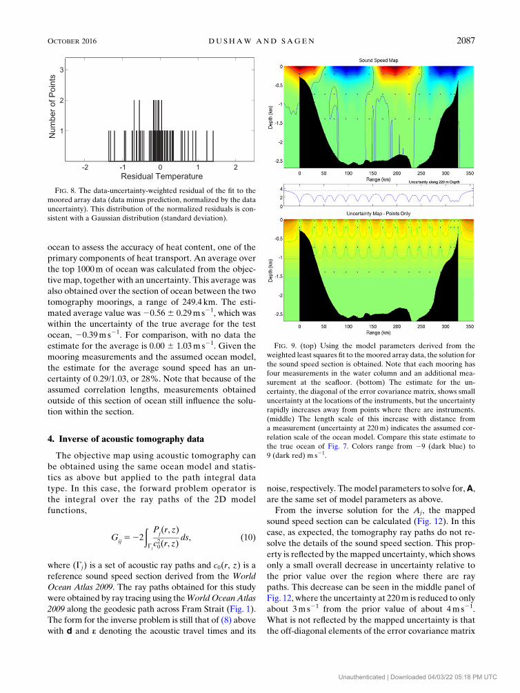
From the inverse solution for the Aj, the mapped

sound speed section can be calculated (Fig. 12). In this

case, as expected, the tomography ray paths do not re-

solve the details of the sound speed section. This prop-

erty is reflected by the mapped uncertainty, which shows

only a small overall decrease in uncertainty relative to

the prior value over the region where there are ray

paths. This decrease can be seen in the middle panel of

Fig. 12, where the uncertainty at 220m is reduced to only

about 3m s21 from the prior value of about 4m s21.

What is not reflected by the mapped uncertainty is that

the off-diagonal elements of the error covariance matrix

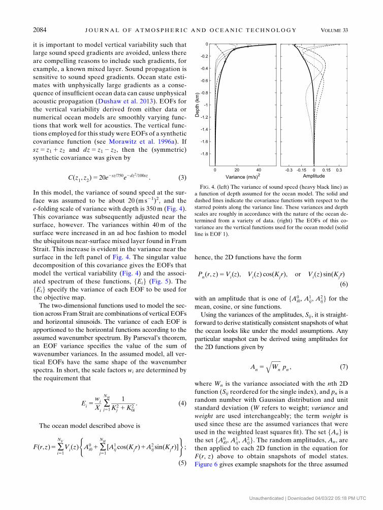
FIG. 8. The data-uncertainty-weighted residual of the fit to the

moored array data (data minus prediction, normalized by the data

uncertainty). This distribution of the normalized residuals is con-

sistent with a Gaussian distribution (standard deviation).

FIG. 9. (top) Using the model parameters derived from the

weighted least squares fit to the moored array data, the solution for

the sound speed section is obtained. Note that each mooring has

four measurements in the water column and an additional mea-

surement at the seafloor. (bottom) The estimate for the un-

certainty, the diagonal of the error covariance matrix, shows small

uncertainty at the locations of the instruments, but the uncertainty

rapidly increases away from points where there are instruments.

(middle) The length scale of this increase with distance from

a measurement (uncertainty at 220m) indicates the assumed cor-

relation scale of the ocean model. Compare this state estimate to

the true ocean of Fig. 7. Colors range from 29 (dark blue) to

9 (dark red) m s21.

OCTOBER 2016 DUSHAW AND SAGEN 2087

Unauthenticated | Downloaded 04/03/22 05:18 PM UTC

are important. The ray paths measure a natural average,

and the correlations of the error matrix express the na-

ture of this average measurement. The average sound

speed and its uncertainty computed over the 0–1000-m-

depth interval and over range was 20.40 6 0.19ms21.

Indeed, the uncertainty of the average is small, even

though the pointwise uncertainty was about 3ms21.

Given the tomography measurements and the assumed

ocean model, the estimate for the average sound speed

has an uncertainty of 0:19/1:03, or 18%.

5. Combined inverse of moored array data andtomography data

In many ways, the point and line integral measure-

ments are complementary, with optimal results obtained

by combining these different data types with the objec-

tive map. The objective map can be applied to both the

point and path integral measurements by merely

‘‘stacking’’ the data (Morawitz et al. 1996a). The data

vector, di, is a vector with the point measurement data

above the travel time data,

di5

"d1n

d2m

#, (11)

and the forward problem operator is just

Gij5

"G1

nj

G2mj

#, (12)

where the superscripts 1 and 2 refer to the point and path

integral measurements, respectively. The objective and

error maps resulting from combining these data types

are given in Fig. 13.

Calculating average sound speed over the

0–1000-m-depth interval and over range obtained a value

of20.396 0.08ms21, in near-perfect agreement with the

true value of20.39. By combining the two data types, the

uncertainty was reduced by more than a factor of 3.

FIG. 10. As in Fig. 9, but assuming a very short correlation length

for the ocean model (top panel of Fig. 3). Away from in-

strumentation, the solution rapidly decreases to zero, and the un-

certainty similarly rapidly increases to the prior variance. Compare

this state estimate to the true ocean of Fig. 7. Colors range from

29 (dark blue) to 9 (dark red) m s21.

FIG. 11. As in Fig. 10, but assuming a very long correlation length

for the ocean model (bottom panel of Fig. 3). The solution is well

correlated across the instruments, and the uncertainty is small

throughout and slowly increases to the prior variance away from

instrumentation. Compare this state estimate to the true ocean of

Fig. 7. Colors range from 29 (dark blue) to 9 (dark red) m s21.

2088 JOURNAL OF ATMOSPHER IC AND OCEAN IC TECHNOLOGY VOLUME 33

Unauthenticated | Downloaded 04/03/22 05:18 PM UTC

Given both the moored array and tomography mea-

surements and the assumed ocean model, the estimate

for the average sound speed has an uncertainty of

0:08/1:03, or 8%. For random sampling with white noise,

the value for the uncertainty improves by the square

root of the number of point measurements. If ocean

variability was random, then a similar improvement in

uncertainty could be obtained by increasing the num-

ber of point measurements by an order of magnitude

(e.g., employ 160, rather than 16, moorings). This

scaling is only approximate for the real ocean, however,

since ocean variability does not usually have a white

spectrum.

6. Objective map of a hydrographic section

The model and objective mapping can be applied to a

zonal section of hydrographic data across Fram Strait.

These data were obtained from the Norwegian Coast

Guard Vessel (CGV) KV Svalbard at the end of

September 2011 over an 8-day interval from 78.21388N,

4.09158W to 77.90438N, 8.61888E (Fig. 14; Sagen and

Beszczynska-Möller 2015). This application provides

both a test of the model against real data and an addi-

tional example of sampling and resolution. These hy-

drographic data have sampling similar to the moored

array but with almost continuous measurements in the

vertical.

The hydrographic section was obtained using 17T-5

expendable bathy thermograph (XBT) casts, nominally

to about 1800-m depth. The manufacturer’s XBT data

acquisition system assigned a nominal salinity profile to

the temperature profile, from which pressure and

sound speed were computed using the Chen–Millero

equation. While the salinity assigned in this way is

imprecise and the Chen–Millero equation is known to

be slightly in error at depth (Dushaw et al. 1993a), for

our purposes the sound speed computed this way was

adequate. Temperature variability is the dominant ef-

fect on sound speed and, as previously noted, data

uncertainties of 1m s21 were assumed to account for

FIG. 12. (top) The solution for the sound speed section obtained

using only acoustic tomography data. (bottom) The estimate for the

uncertainty decreases only slightly in regions where there are ray

paths; the off-diagonal elements of the error covariance are impor-

tant in this case. Compare this state estimate to the true ocean of

Fig. 7. Colors range from 29 (dark blue) to 9 (dark red) m s21.

FIG. 13. (top) The solution for the sound speed section obtained

using both moored and acoustic tomography data. (bottom) The

estimate for the uncertainty is considerably reduced with the

smallest uncertainty where there are point measurements. Com-

pare this state estimate to the true ocean of Fig. 7. Colors range

from 29 (dark blue) to 9 (dark red) m s21.

OCTOBER 2016 DUSHAW AND SAGEN 2089

Unauthenticated | Downloaded 04/03/22 05:18 PM UTC

internalwaves andother unresolved variability. Theprofiles

of sound speed were decimated to values at 10-m intervals

by cubic spline interpolation with little loss of information.

The model employed here for objective mapping

accounted for the observations within data uncertainty.

This fit was made to data relative to the average sound

speed profile. The fit demonstrated that the model

was adequate to account for the characteristics of tem-

perature variability within Fram Strait, at least for this

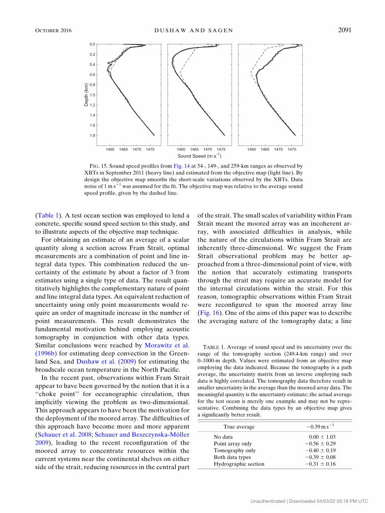
sample size of one (Fig. 15). The spacing of the hydro-

graphic profiles was about 18 km, however, and it was

readily apparent that adjacent profiles were frequently

uncorrelated. Nevertheless, the spatial characteristics of

the mapped hydrography section were roughly consis-

tent with the vertical and horizontal scales assumed for

the objective map (compare the mapped actual ocean

sound speed section of Fig. 14 with the three realizations

of Fig. 6). Profiles of three XBT casts are compared to

the objective map fit in Fig. 15.

The hydrographic sampling was applied to the test

ocean pattern of Fig. 7. Mapped with the hydro-

graphic sampling, the computed average sound

speed over the 0–1000-m-depth interval and over

the range of the tomography path had a value

of 20.31 6 0.16m s21. The average value estimated

this way was consistent with the true value, with

uncertainty slightly less than the uncertainty obtained

using only the tomography data. Inasmuch as the

moored array and hydrographic sampling character-

istics are similar, it is apparent that combining

hydrographic and tomography data for this map

would result in significantly smaller uncertainty.

7. Discussion

This simplified study was separated from the compli-

cations of the real ocean to focus on the specific issue of

point-versus-line-average measurements of a scalar

quantity and the resolution these data types have for a

particular ocean model. While simplified, an attempt

was made to place the study within the environment of

Fram Strait in a realistic way. One aim of this study was

partly to use it as a stepping-stone toward a more com-

prehensive study of Fram Strait oceanography using the

point and line integral data types, both of which are now

available. Future steps in this analysis are to employ the

actual moored array and tomography measurements,

together with CTD and glider sections, and other data,

to determine an accurate three-dimensional statistical

model for Fram Strait variability. Such a model can then

be applied to the available data to obtain ‘‘best esti-

mates’’ for the variability.

This study adopted a particular ocean model based on

sinusoids horizontally and covariance EOFs vertically.

Assumptions were also made about these functions and

their associated statistics for the variability of a scalar

variable (sound speed) in range and depth. Any results

or conclusions drawn from this study depend on the

model assumptions. Nevertheless, the study employs a

reasonable ocean model with self-consistent calcula-

tions and obtains results in that context. Indeed, the

horizontal and vertical scales assumed for the ocean

model were found to be consistent with data obtained

from a hydrographic section across Fram Strait. The key

quantities resulting from these calculations were the

estimated uncertainties for range- and-depth-averaged

sound speed for point measurements alone, tomography

measurements alone, and both data types combined

FIG. 14. (top) An objectivemap of a sound speed section derived

from hydrography data obtained across Fram Strait along the

southern zonal ACOBAR acoustic path (Fig. 1) in late September

2011. The inverse is relative to the path-averaged sound speed

profile. (bottom) The estimate for the uncertainty is considerably

reduced where hydrographic profiles were obtained. With spacing

of about 18 km, the sound speed fluctuations between adjacent

profiles are uncorrelated. Colors range from 29 (dark blue) to

9 (dark red) m s21.

2090 JOURNAL OF ATMOSPHER IC AND OCEAN IC TECHNOLOGY VOLUME 33

Unauthenticated | Downloaded 04/03/22 05:18 PM UTC

(Table 1). A test ocean section was employed to lend a

concrete, specific sound speed section to this study, and

to illustrate aspects of the objective map technique.

For obtaining an estimate of an average of a scalar

quantity along a section across Fram Strait, optimal

measurements are a combination of point and line in-

tegral data types. This combination reduced the un-

certainty of the estimate by about a factor of 3 from

estimates using a single type of data. The result quan-

titatively highlights the complementary nature of point

and line integral data types. An equivalent reduction of

uncertainty using only point measurements would re-

quire an order of magnitude increase in the number of

point measurements. This result demonstrates the

fundamental motivation behind employing acoustic

tomography in conjunction with other data types.

Similar conclusions were reached by Morawitz et al.

(1996b) for estimating deep convection in the Green-

land Sea, and Dushaw et al. (2009) for estimating the

broadscale ocean temperature in the North Pacific.

In the recent past, observations within Fram Strait

appear to have been governed by the notion that it is a

‘‘choke point’’ for oceanographic circulation, thus

implicitly viewing the problem as two-dimensional.

This approach appears to have been the motivation for

the deployment of the moored array. The difficulties of

this approach have become more and more apparent

(Schauer et al. 2008; Schauer and Beszczynska-Möller2009), leading to the recent reconfiguration of the

moored array to concentrate resources within the

current systems near the continental shelves on either

side of the strait, reducing resources in the central part

of the strait. The small scales of variability within Fram

Strait meant the moored array was an incoherent ar-

ray, with associated difficulties in analysis, while

the nature of the circulations within Fram Strait are

inherently three-dimensional. We suggest the Fram

Strait observational problem may be better ap-

proached from a three-dimensional point of view, with

the notion that accurately estimating transports

through the strait may require an accurate model for

the internal circulations within the strait. For this

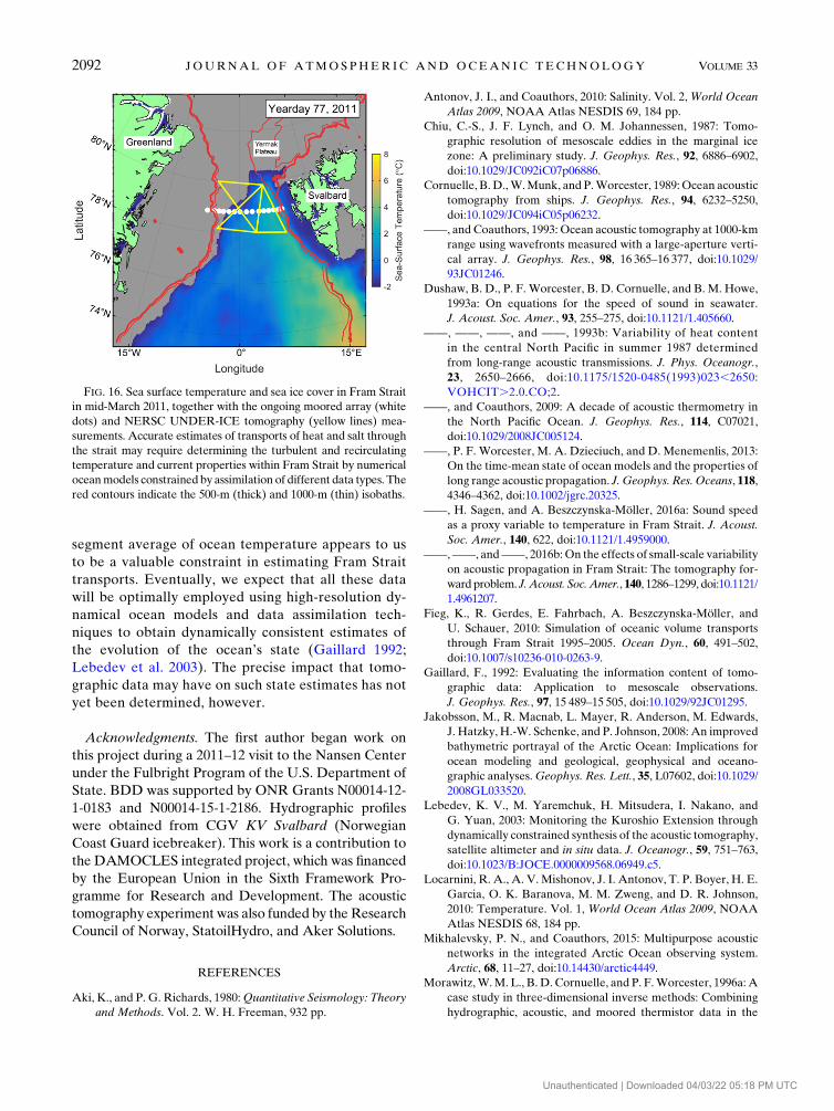
reason, tomographic observations within Fram Strait

were reconfigured to span the moored array line

(Fig. 16). One of the aims of this paper was to describe

the averaging nature of the tomography data; a line

FIG. 15. Sound speed profiles from Fig. 14 at 54-, 149-, and 259-km ranges as observed by

XBTs in September 2011 (heavy line) and estimated from the objective map (light line). By

design the objective map smooths the short-scale variations observed by the XBTs. Data

noise of 1 m s21 was assumed for the fit. The objective map was relative to the average sound

speed profile, given by the dashed line.

TABLE 1. Average of sound speed and its uncertainty over the

range of the tomography section (249.4-km range) and over

0–1000-m depth. Values were estimated from an objective map

employing the data indicated. Because the tomography is a path

average, the uncertainty matrix from an inverse employing such

data is highly correlated. The tomography data therefore result in

smaller uncertainty in the average than the moored array data. The

meaningful quantity is the uncertainty estimate; the actual average

for the test ocean is merely one example and may not be repre-

sentative. Combining the data types by an objective map gives

a significantly better result.

True average 20.39m s21

No data 0.00 6 1.03

Point array only 20.56 6 0.29

Tomography only 20.40 6 0.19

Both data types 20.39 6 0.08

Hydrographic section 20.31 6 0.16

OCTOBER 2016 DUSHAW AND SAGEN 2091

Unauthenticated | Downloaded 04/03/22 05:18 PM UTC

segment average of ocean temperature appears to us

to be a valuable constraint in estimating Fram Strait

transports. Eventually, we expect that all these data

will be optimally employed using high-resolution dy-

namical ocean models and data assimilation tech-

niques to obtain dynamically consistent estimates of

the evolution of the ocean’s state (Gaillard 1992;

Lebedev et al. 2003). The precise impact that tomo-

graphic data may have on such state estimates has not

yet been determined, however.

Acknowledgments. The first author began work on

this project during a 2011–12 visit to the Nansen Center

under the Fulbright Program of the U.S. Department of

State. BDD was supported by ONR Grants N00014-12-

1-0183 and N00014-15-1-2186. Hydrographic profiles

were obtained from CGV KV Svalbard (Norwegian

Coast Guard icebreaker). This work is a contribution to

the DAMOCLES integrated project, which was financed

by the European Union in the Sixth Framework Pro-

gramme for Research and Development. The acoustic

tomography experiment was also funded by the Research

Council of Norway, StatoilHydro, and Aker Solutions.

REFERENCES

Aki, K., and P. G. Richards, 1980:Quantitative Seismology: Theory

and Methods. Vol. 2. W. H. Freeman, 932 pp.

Antonov, J. I., and Coauthors, 2010: Salinity. Vol. 2, World Ocean

Atlas 2009, NOAA Atlas NESDIS 69, 184 pp.

Chiu, C.-S., J. F. Lynch, and O. M. Johannessen, 1987: Tomo-

graphic resolution of mesoscale eddies in the marginal ice

zone: A preliminary study. J. Geophys. Res., 92, 6886–6902,

doi:10.1029/JC092iC07p06886.

Cornuelle, B.D.,W.Munk, and P.Worcester, 1989:Ocean acoustic

tomography from ships. J. Geophys. Res., 94, 6232–5250,

doi:10.1029/JC094iC05p06232.

——, and Coauthors, 1993: Ocean acoustic tomography at 1000-km

range using wavefronts measured with a large-aperture verti-

cal array. J. Geophys. Res., 98, 16 365–16 377, doi:10.1029/

93JC01246.

Dushaw, B. D., P. F. Worcester, B. D. Cornuelle, and B. M. Howe,

1993a: On equations for the speed of sound in seawater.

J. Acoust. Soc. Amer., 93, 255–275, doi:10.1121/1.405660.

——, ——, ——, and ——, 1993b: Variability of heat content

in the central North Pacific in summer 1987 determined

from long-range acoustic transmissions. J. Phys. Oceanogr.,

23, 2650–2666, doi:10.1175/1520-0485(1993)023,2650:

VOHCIT.2.0.CO;2.

——, and Coauthors, 2009: A decade of acoustic thermometry in

the North Pacific Ocean. J. Geophys. Res., 114, C07021,

doi:10.1029/2008JC005124.

——, P. F. Worcester, M. A. Dzieciuch, and D. Menemenlis, 2013:

On the time-mean state of ocean models and the properties of

long range acoustic propagation. J. Geophys. Res. Oceans, 118,

4346–4362, doi:10.1002/jgrc.20325.

——, H. Sagen, and A. Beszczynska-Möller, 2016a: Sound speed

as a proxy variable to temperature in Fram Strait. J. Acoust.

Soc. Amer., 140, 622, doi:10.1121/1.4959000.——,——, and——, 2016b:On the effects of small-scale variability

on acoustic propagation in Fram Strait: The tomography for-

ward problem. J. Acoust. Soc.Amer., 140, 1286–1299, doi:10.1121/

1.4961207.

Fieg, K., R. Gerdes, E. Fahrbach, A. Beszczynska-Möller, andU. Schauer, 2010: Simulation of oceanic volume transports

through Fram Strait 1995–2005. Ocean Dyn., 60, 491–502,

doi:10.1007/s10236-010-0263-9.

Gaillard, F., 1992: Evaluating the information content of tomo-

graphic data: Application to mesoscale observations.

J. Geophys. Res., 97, 15 489–15 505, doi:10.1029/92JC01295.

Jakobsson, M., R. Macnab, L. Mayer, R. Anderson, M. Edwards,

J. Hatzky, H.-W. Schenke, and P. Johnson, 2008: An improved

bathymetric portrayal of the Arctic Ocean: Implications for

ocean modeling and geological, geophysical and oceano-

graphic analyses.Geophys. Res. Lett., 35, L07602, doi:10.1029/

2008GL033520.

Lebedev, K. V., M. Yaremchuk, H. Mitsudera, I. Nakano, and

G. Yuan, 2003: Monitoring the Kuroshio Extension through

dynamically constrained synthesis of the acoustic tomography,

satellite altimeter and in situ data. J. Oceanogr., 59, 751–763,

doi:10.1023/B:JOCE.0000009568.06949.c5.

Locarnini, R. A., A. V. Mishonov, J. I. Antonov, T. P. Boyer, H. E.

Garcia, O. K. Baranova, M. M. Zweng, and D. R. Johnson,

2010: Temperature. Vol. 1, World Ocean Atlas 2009, NOAA

Atlas NESDIS 68, 184 pp.

Mikhalevsky, P. N., and Coauthors, 2015: Multipurpose acoustic

networks in the integrated Arctic Ocean observing system.

Arctic, 68, 11–27, doi:10.14430/arctic4449.

Morawitz,W.M. L., B. D. Cornuelle, and P. F.Worcester, 1996a:A

case study in three-dimensional inverse methods: Combining

hydrographic, acoustic, and moored thermistor data in the

FIG. 16. Sea surface temperature and sea ice cover in Fram Strait

in mid-March 2011, together with the ongoing moored array (white

dots) and NERSC UNDER-ICE tomography (yellow lines) mea-

surements. Accurate estimates of transports of heat and salt through

the strait may require determining the turbulent and recirculating

temperature and current properties within Fram Strait by numerical

oceanmodels constrainedby assimilation of different data types. The

red contours indicate the 500-m (thick) and 1000-m (thin) isobaths.

2092 JOURNAL OF ATMOSPHER IC AND OCEAN IC TECHNOLOGY VOLUME 33

Unauthenticated | Downloaded 04/03/22 05:18 PM UTC

Greenland Sea. J. Atmos. Oceanic Technol., 13, 659–679,

doi:10.1175/1520-0426(1996)013,0659:ACSITD.2.0.CO;2.

——, P. J. Sutton, P. F.Worcester, B. D. Cornuelle, J. F. Lynch, and

R. Pawlowicz, 1996b: Three-dimensional observations of a

deep convective chimney in the Greenland Sea during win-

ter 1988/89. J. Phys. Oceanogr., 26, 2316–2343, doi:10.1175/

1520-0485(1996)026,2316:TDOOAD.2.0.CO;2.

Munk, W. H., P. F. Worcester, and C. Wunsch, 1995: Ocean

Acoustic Tomography. Cambridge University Press, 433 pp.

Naugolnykh, K. A., O. M. Johannessen, I. B. Esipov, O. B.

Ovchinnikov, Y. I. Tuzkilkin, and V. V. V. V. Zosimov, 1998:

Numerical simulation of remote acoustic sensing of ocean

temperature in the Fram Strait environment. J. Acoust. Soc.

Amer., 104, 738–746, doi:10.1121/1.423349.

Nurser, A. J. G., and S. Bacon, 2014: The Rossby radius in

the Arctic Ocean. Ocean Sci., 10, 967–975, doi:10.5194/

os-10-967-2014.

Sagen, H., and A. Beszczynska-Möller, 2015: Fram Strait/

ACOBAR: XBT measurements and derived values - Fram

Strait - September 2011. NERSC TDS Server, accessed 13

September 2016. [Available online at http://thredds.nersc.no/

thredds/arcticData/fram-strait.html?dataset=NERSC_ARC_

PHYS_OBS_XBT_2011_v1.]

——, B. D. Dushaw, E. K. Skarsoulis, D. Dumont, M. A.

Dzieciuch, and A. Beszczynska-Möller, 2016: Time series of

temperature in Fram Strait determined from the 2008–2009

DAMOCLES acoustic tomography measurements and an

ocean model. J. Geophys. Res. Oceans, 121, 4601–4617,

doi:10.1002/2015JC011591.

Schauer, U., and A. Beszczynska-Möller, 2009: Problems with es-

timation and interpretation of oceanic heat transport con-

ceptual remarks for the case of Fram Strait in the Arctic

Ocean. Ocean Sci., 5, 487–494, doi:10.5194/os-5-487-2009.

——, ——, W. Walczowski, E. Fahrbach, J. Plechura, and

E. Hansen, 2008: Variation of measured heat flow through the

Fram Strait between 1997 and 2006. Arctic–Subarctic Ocean

Fluxes, R. R. Dickson, J. Meineke, and P. Rhines, Eds.,

Springer, 65–85, doi:10.1007/978-1-4020-6774-7_4.

Skarsoulis, E., G. Piperakis, M. Kalogerakis, H. Sagen, S. Haugen,

A. Beszczynska-Möller, and P.Worcester, 2010: Tomographic

inversions from the Fram Strait 2008–9 experiment. Pro-

ceedings of the 10th European Conference on Underwater

Acoustics, ECUA 2010, T. Akal, Ed., Vol. 1, Ofset Basim

Yayin A.S., 265–271.

Smedsrud, L. H., A. Sirevaag, K. Kloster, A. Sorteberg, and

S. Sandven, 2011: Recent wind driven high sea ice area export

in the Fram Strait contributes to Arctic sea ice decline.

Cryosphere, 5, 821–829, doi:10.5194/tc-5-821-2011.

von Appen, W.-J., U. Schauer, R. Somavilla, E. Bauerfeind, and

A. Beszczynska-Möller, 2015: Exchange of warming deep

waters across Fram Strait. Deep-Sea Res. I, 103, 86–100,

doi:10.1016/j.dsr.2015.06.003.

OCTOBER 2016 DUSHAW AND SAGEN 2093

Unauthenticated | Downloaded 04/03/22 05:18 PM UTC