A Collection of Computer Vision

Algorithms Capable of Detecting Linear

Infrastructure for the Purpose of UAV

Control

Evan McLean Smith

Thesis submitted to the faculty of the Virginia Polytechnic Institute and State

University in partial fulfillment of the requirements for the degree of

Master of Science

In

Mechanical Engineering

Kevin B. Kochersberger

A. Lynn Abbott

Tomonari Furukawa

April 20th

, 2016

Blacksburg, VA

Keywords: autonomous navigation, computer vision, linear infrastructure, machine

learning, unmanned aerial vehicle (UAV)

Copyright 2016 ©

A Collection of Computer Vision Algorithms

Capable of Detecting Linear Infrastructure

for the Purpose of UAV Control

Evan McLean Smith

ABSTRACT

One of the major application areas for UAVs is the automated traversing and

inspection of infrastructure. Much of this infrastructure is linear, such as roads, pipelines,

rivers, and railroads. Rather than hard coding all of the GPS coordinates along these

linear components into a flight plan for the UAV to follow, one could take advantage of

computer vision and machine learning techniques to detect and travel along them. With

regards to roads and railroads, two separate algorithms were developed to detect the angle

and distance offset of the UAV from these linear infrastructure components to serve as

control inputs for a flight controller. The road algorithm relied on applying a Gaussian

SVM to segment road pixels from rural farmland using color plane and texture data. This

resulted in a classification accuracy of 96.6% across a 62 image dataset collected at

Kentland Farm. A trajectory can then be generated by fitting the classified road pixels to

polynomial curves. These trajectories can even be used to take specific turns at

intersections based on a user defined turn direction and have been proven through

hardware-in-the-loop simulation to produce a mean cross track error of only one road

width. The combined segmentation and trajectory algorithm was then implemented on a

PC (i7-4720HQ 2.6 GHz, 16 GB RAM) at 6.25 Hz and a myRIO 1900 at 1.5 Hz proving

its capability for real time UAV control. As for the railroad algorithm, template matching

was first used to detect railroad patterns. Upon detection, a region of interest around the

matched pattern was used to guide a custom edge detector and Hough transform to detect

the straight lines on the rails. This algorithm has been shown to detect rails correctly, and

thus the angle and distance offset error, on all images related to the railroad pattern

template and can run at 10 Hz on the aforementioned PC.

A Collection of Computer Vision Algorithms

Capable of Detecting Linear Infrastructure

for the Purpose of UAV Control

Evan McLean Smith

GENERAL AUDIENCE ABSTRACT

Unmanned aerial vehicles (UAVs) have the potential to change many aspects of

society for the better. Some of their more popular modern applications include package

delivery and infrastructure inspection. But how does a UAV currently perform these

tasks? Generally speaking, UAVs use an array of sensors, including a global positioning

system (GPS) sensor and a compass, to detect where they are in their environment and

where they are going. Using flight control software, an engineer can tell the UAV where

to go by placing various GPS coordinates on a map for the UAV to follow in a sequential

order at mission time. For example, this could mean marking the GPS coordinate of

someone’s house that requires a package delivery or a specific section of railroad that

needs inspection. However, the roads that the UAV would fly above to get to the house or

the railroad the UAV would fly along to get to the inspection site provide natural visual

cues that as humans, would allow us to reach these destinations without a GPS. These

cues can be detected by UAVs as well by mounting a camera onboard. Upon sending the

images from this camera to a computer on the UAV, image processing and other

programming techniques can be used to find where the roads or railroads are in the

image. The basis of my work was developing software packages capable of such a task.

To detect roads, examples showing the color and texture of the road were shown to the

computer to help it distinguish between road and non-road image sections. Once it

learned what a road looked like and found it, it was then able to tell the UAV where to

move to align itself with the road. For railroads, a small template image containing a

small portion of a railroad was compared with the image to try to find matches. If a match

was found, then a second algorithm which looked for the rails (approximated as straight

lines) was implemented near the match location. Both algorithms were shown to be

accurate to within a few pixels and run quickly setting the stage for future application.

`iii

DEDICATION

I first would like to dedicate my thesis to my loving parents, Joyce and Mac

Smith, who supported me in so many ways throughout my college career. They always

put a positive spin on things and regardless of how my weeks went at school, I knew that

I had a safe refuge with them.

I would next like to dedicate my thesis to my amazing fiancé, Victoria McClintic-

Church, who has been by my side through all of the challenges this degree has brought

upon me. She has made a huge impact on several important decisions throughout my

graduate career and I am so lucky to have had her with me through this process.

My final dedication is to my friends both in and outside of school whose names

are too numerous to list, but whose mark on my degree cannot be missed. Whether it was

academic assistance, a prayer, or just hanging out and forgetting about the struggles for a

while, all of you are responsible for my level of positivity and success.

`iv

ACKNOWLEDGEMENTS

My gratitude first and foremost must go to my advisor Dr. Kochersberger. He has

stood out as one of the best advisors I could have asked for mostly because he, above all

other professors I have come to know intimately, puts his students first. Given that

academia generally rewards advisors with a more selfish behavior, I have a great respect

for him maintaining this stance. Beyond this however, he has lived up to all other

expectations one would have of an advisor. He has worked very hard every semester to

ensure I have funding, that I am working on a project that is both meaningful and

something I am passionate about, and has pushed me to take the challenging coursework

necessary to succeed in the modern robotics community. I have been very lucky to have

him as a mentor in graduate school and know the lessons learned through working with

him have well prepared me for my professional career.

My next set of acknowledgements go to several lab members: Haseeb Chaudhry

in part for his assistance on the AIAA project and for being an excellent peer mentor to

me, Gordon Christie for countless computer vision and machine learning

recommendations, Matthew Frauenthal for introducing me to the field I have come to

have such passion for, Andrew Morgan for his insight on aircraft design, Justin Stiltner

for being all around wealth of knowledge, and Danny Whitehurst for practically facing

every graduate school challenge with and for always being there to bounce another idea

off of.

Finally, I would like to thank my major corporate sponsor, Jennifer Player of

Bihrle Applied Research. Through her initial financial assistance, data provisions, and

project support, I was able to work on cutting edge UAV research and develop a stem

project that formed the backbone of my thesis work.

`v

ATTRIBUTION

While most of the work presented in this thesis is that of my own, I would not

have accomplished all that I did without the research and writing of a few past and

present individuals from the Unmanned Systems Lab.

Chapter 3: Road Detection

Haseeb Chaudhry, Ph. D. candidate, is currently working on his doctoral

Mechanical Engineering degree in the Unmanned Systems Lab at Virginia Tech. He is

well versed in control theory and aircraft design and was responsible for the controls

portion of the AIAA work.

Chapter 4: Railroad Detection

Matthew Frauenthal, M.S., is a Mechanical Engineering graduate from the

Unmanned Systems lab at Virginia Tech. He is currently an engineer at Kollmorgen

Corporation responsible for motor prototyping and manufacturing assistance. His work

provided much of the dataset used for the railroad algorithm development.

`vi

TABLE OF CONTENTS

1. INTRODUCTION ................................................................................................ 1

2. BACKGROUND .................................................................................................. 6

2.1 Unmanned Aerial Vehicles ................................................................................. 6

2.2 Camera Concepts .............................................................................................. 11

2.3 Computer Vision Concepts ............................................................................... 15

2.3.1 Color Spaces .............................................................................................. 16

2.3.2 Filters, Edges, and Texture ........................................................................ 19

2.3.3 Binary Operations ...................................................................................... 21

2.3.4 Hough Transform ....................................................................................... 24

2.3.5 Color Pattern Matching .............................................................................. 27

2.4 Machine Learning Algorithms .......................................................................... 29

2.4.1 Unsupervised Learning .............................................................................. 29

2.4.2 Supervised Learning .................................................................................. 31

3. ROAD DETECTION ......................................................................................... 35

3.1 Road Detection and UAV Trajectory Development Algorithm ....................... 36

3.1.1 Road Segmentation .................................................................................... 36

3.1.2 Road Class Detection ................................................................................. 41

3.1.3 Trajectory Line and Control Input Calculation .......................................... 45

3.1.4 Results ........................................................................................................ 49

3.2 Additional Work ............................................................................................... 51

3.2.1 FPGA Algorithm Development ................................................................. 51

3.2.2 Camera Selection ....................................................................................... 56

3.2.3 Airplane Payload and Ground Station Design ........................................... 58

3.2.4 Qualitative Results ..................................................................................... 61

`vii

3.2.5 HIL Simulation .......................................................................................... 64

4. RAILROAD DETECTION ................................................................................ 68

4.1 Background ....................................................................................................... 68

4.2 Railroad Detection Algorithm ........................................................................... 74

4.2.1 Railroad Template Matching ..................................................................... 74

4.2.2 Rail Detection ............................................................................................ 78

4.2.3 Results ........................................................................................................ 80

4.3 Additional Work ............................................................................................... 86

4.3.1 Altitude Resolution Study .......................................................................... 86

4.3.2 Ground Station Design ............................................................................... 89

4.3.3 Shadow Resistant Detection ...................................................................... 94

5. CONCLUSIONS AND RECOMMENDATIONS ............................................ 95

REFERENCES ........................................................................................................... 98

`viii

LIST OF FIGURES

Figure 1. Remote Infrastructure Examples ................................................................... 2

Figure 2. Summary of Thesis Objective ....................................................................... 4

Figure 3. Examples of Various UAV Platforms ........................................................... 6

Figure 4. Standard Level 3 Autonomy RPV Fixed Wing System ................................ 8

Figure 5. Standard Level 3 Autonomy RPV Multirotor System .................................. 9

Figure 6. Level 5 Autonomy RPV System for Following Linear Infrastructure ........ 10

Figure 7. Diagram of a Digital Camera ...................................................................... 11

Figure 8. Effect of GSD on Image Quality ................................................................. 13

Figure 9. Consequences of Rolling and Global Shutters for Moving Cameras .......... 15

Figure 10. HSL and HSV Color Space Cylindrical Models ....................................... 18

Figure 11. Lab Color Space Spherical Model ............................................................. 18

Figure 12. Examples of Common Computer Vision Filters ....................................... 19

Figure 13. XY Sobel Filter.......................................................................................... 20

Figure 14. Summary of Hough Transform for Line Detection ................................... 26

Figure 15. Goal of Color Pattern Matching ................................................................ 27

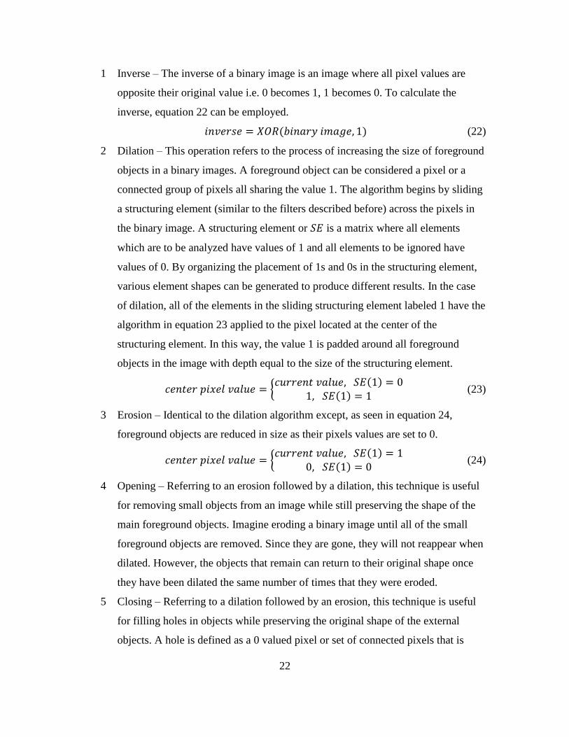
Figure 16. Flow of kMeans Algorithm ....................................................................... 30

Figure 17. Support Vector Machine Basics ................................................................ 32

Figure 18. Original and Labeled Road Images ........................................................... 37

Figure 19. Visualization of sequential feature selection technique ............................ 38

Figure 20. Down selection of top sequential feature matching features ..................... 39

Figure 21. Final Segmentation Features and SVM Results ........................................ 40

Figure 22. Camera Parameters and FOV Visualization (Altitude = 50 m) ................. 41

Figure 23. Visualization of Road Class Detection Features ....................................... 42

Figure 24. Generation of the Trajectory Line ............................................................. 45

Figure 25. Generation of Unique Trajectory Lines Based on Desired Direction ....... 47

Figure 26. Definition of Direction Criteria ................................................................. 48

Figure 27. myRIO FPGA kNN Algorithm on LabVIEW Block Diagram ................. 56

Figure 28. Final Camera Choice (Basler acA1920-155uc) ......................................... 58

Figure 29. Road Tracking Ground Station Front Panel .............................................. 61

Figure 30. Road Detection Result for Single Road..................................................... 61

`ix

Figure 31. Road Detection Result for Single Road (Occlusion and Mislabeling) ...... 62

Figure 32. Road Detection Result for Single Road (Heavy Shadow)......................... 62

Figure 33. Road Detection Result a Three Way Intersection (Direction: Straight) .... 63

Figure 34. Road Detection Result a Three Way Intersection (Direction: Left) .......... 63

Figure 35. Road Detection Result a Four Way Intersection (Direction: Left) ............ 63

Figure 36. Road Detection and Tracking HIL Simulation Set-Up ............................. 64

Figure 37. HIL Simulation Segmentation ................................................................... 65

Figure 38. HIL Simulation Trajectory ........................................................................ 65

Figure 39. HIL Simulation UAV Trajectory vs. Road Ground Truth ........................ 66

Figure 40. Components of a Railroad ......................................................................... 68

Figure 41. Example of a Rail Kink ............................................................................. 69

Figure 42. Railroad Geometry Inspection Car ............................................................ 69

Figure 43. Viable UAV Example for Railroad Inspection ......................................... 70

Figure 44. Railroad Grayscale Histogram Equalization ............................................. 71

Figure 45. LLPD Filter Bank Applied to Histogram Image ....................................... 72

Figure 46. Hough Transform Detecting Railroad Obstacles ...................................... 72

Figure 47. First Rail Detection Mask Bank Iteration .................................................. 73

Figure 48. Refined Rail Detection Mask Bank Iteration ............................................ 73

Figure 49. Examples of Poor Templates for Railroad Detection ................................ 75

Figure 50. Rail-Tie Color Pattern Matching Template Examples .............................. 76

Figure 51. Detected Rail-Tie Pattern Matches on Test Image .................................... 77

Figure 52. Detected Railroad Profile via ROI Technique ........................................... 78

Figure 53. Rail Edge Detection Algorithm ................................................................. 79

Figure 54. Successful Result of Rail Detection Algorithm......................................... 80

Figure 55. Template Matching Pyramid for Different Resolutions or Altitudes ........ 81

Figure 56. Trend of Run Time vs. Resolution ............................................................ 82

Figure 57. Performance Curve of Angled Rail Detection vs. Resolution ................... 83

Figure 58. Vertical Rail Detection at 480p ................................................................. 84

Figure 59. Angled Rail Detection at 480p .................................................................. 84

Figure 60. Horizontal Rail Detection at 480p ............................................................. 85

Figure 61. Mosaic of Railroads Used for Camera Testing ......................................... 85

`x

Figure 62. Tie Plate Spike Inspection Image (Altitude: 5 m) ..................................... 87

Figure 63. Tie Plate Spike Inspection Image (Altitude: 8 m) ..................................... 87

Figure 64. Tie Plate Spike Inspection Image (Altitude: 14 m) ................................... 87

Figure 65. Tie Plate Spike Inspection Image (Altitude: 17 m) ................................... 88

Figure 66. Tie Plate Spike Inspection Image (Altitude: 23 m) ................................... 88

Figure 67. Five Parallel Loops for Railroad Inspection Ground Station .................... 89

Figure 68. Railroad Ground Station Front Panel ........................................................ 91

Figure 69. Acquisition Control Tabs - Real Time w/ Camera .................................... 91

Figure 70. Acquisition Control Tabs - Testing w/ Video and Images ........................ 92

Figure 71. Detection Feedback and Tuning Tabs ....................................................... 93

Figure 72. Defect Detector Tab .................................................................................. 94

Figure 73. Results from Matlab entropyfilt Function ................................................. 95

Figure 74. Example of SLIC Superpixel Segmentation of Road Image ..................... 96

`xi

LIST OF TABLES

Table 1. Cluster Labels to Keep/Remove Based on Desired Direction ...................... 48

Table 2. Results Comparing Image Resolution and Algorithm Run Time ................. 50

Table 3. Results Comparing Image Resolution and Algorithm Run Time ................. 51

Table 4. Xilinx Z-7010 FPGA Resources ................................................................... 53

Table 5. Aircraft Parameters Used for Deriving Image Overlap ................................ 57

Table 6. List of Basler Camera Specifications............................................................ 58

Table 7. Main Components of Aircraft Payload and Ground Station......................... 59

Table 8. Test Image Resolutions for Railroad Algorithm Evaluation ........................ 80

Table 9. Railroad Algorithm Run Times vs. Resolution ............................................ 81

Table 10. Railroad Algorithm Detection Accuracy vs. Resolution and Angle ........... 82

Table 11. Altitudes Tested for Railroad Inspection GSD ........................................... 86

`xii

NOMENCLATURE

𝐴𝑙𝑡: Relative altitude of a UAV with respect to the ground (m)

𝐷: Distance on the ground visible by the nadir view UAV camera (m)

∆: Distance offset between the UAV and the center of the linear infrastructure (m)

𝑓: Focal length of the camera lens (mm)

𝐹𝑃𝑆: Frame rate of the camera (frames per second)

𝐹𝑂𝑉: Angular field of view of the camera lens (deg°)

𝜃: Angular offset between the UAV and the linear infrastructure (deg°)

𝐺𝑆𝐷: Ground sample distance of the images taken by the camera (cm/pixel)

𝑂: Desired image overlap between sequentially taken UAV images (%)

𝑅: Resolution of the camera in a particular imaging sensor dimension (pixels)

𝑉: Ground speed of the UAV (m/s)

1

1. INTRODUCTION

Arguably one of the greatest achievements in modern human history has been the

advancement of ground transportation systems and infrastructure. The arteries of these

systems include roads, railroads, pipelines, and power lines; each one having served to

accelerate the growth of civilization and human ideas on a global scale [1-4]. While

major innovations including air travel, the personal computer, and smartphones have

mitigated some of their original benefits, each form of infrastructure still has an important

place in the 21st century. Roads and highways are the lifeblood of day to day

transportation for much of the developed world and allow us to travel previously

unmanageable distances on a daily basis to reach our homes and places of work while

simultaneously facilitating the transport of goods and services on previously unheard of

scales. Railroads still stand as a viable means of travel with major speed benefits in areas

where high speed rail has been installed. More importantly, railroads provide a very cost

effective means to transport heavy cargo across long distances when compared to other

shipping methods. Pipelines are the energy lifelines that keep the modern world running

through the transport of crude oil, natural gas, and natural gas liquids. They are the reason

that approximately 390 million gallons of gasoline reach their destinations every day in

the United States alone and are still responsible for a large sector of electric power

production [5]. Finally, power lines provide us with a steady supply of electrical energy

which without overstatement drives every facet of modern life.

While the main purpose of these infrastructure systems may be obvious, there are

two less obvious realizations that can be made. The first idea which must be addressed is

that the failure of even one of these systems would be devastating to the other three. The

only cog in the chain preventing such disaster is the inspection, repair, and upgrade of

these systems on a regular basis. Unfortunately, infrequent inspection and high repair

costs often prevent such maintenance to occur in a timely fashion. This is especially true

of railroads, which can rarely be scanned by track monitoring vehicles more than once a

year. In fact, aside from roads, accessing many of these pieces of infrastructure can prove

challenging whether it be due to the remote locations they can reside in or because the

equipment necessary to perform inspections and repairs is difficult to deploy as seen in

2

Figure 1 [6, 7]. These issues are an important first realization to come to terms with, but

there is another realization which can be made leading to potential applications.

Figure 1. Remote Infrastructure Examples - Example of remote pipeline (left) and

power lines (right) presenting inspection and repair challenges

This second non-obvious idea relies on the geometric and geographic nature of

these infrastructure components. From a geometric standpoint, they are generally linear

in nature. This is important because unlike natural formations like forests and lakes, they

have defined paths which could be taken. From a geographic standpoint, they are routes

from one location to another. The presence of any of these components in a previously

untouched landscape provide a logical direction to travel along to reach some destination

where few navigational queues would have existed before. One can imagine being lost in

the wilderness and upon coming across one of these structures, taking advantage of the

linear geometry to define a simple path to follow. Combining this idea with the

geographic knowledge that they will likely lead to some desired destination (in this case

civilization) shows the power of these structures as navigational tools. So now that we

have addressed that these structures are difficult to inspect and provide directional

queues, what can be done with this knowledge?

Enter the modern unmanned aerial vehicle (UAV), defined as any aircraft without

a human operator or passenger physically onboard. This class of aircraft has seen major

advancement outside military application since the early 21st century due to a wide

variety of factors. The three most important, however, have been the downsizing of

powerful computer components, advances in the electronics and software that make these

aircraft possible (lithium batteries, inertial measurement units (IMUs), global positioning

3

system (GPS) chips, electric propulsion systems, etc.), and the overall reduced cost to

produce the aforementioned technologies. This has led to a surge in UAV interest in the

commercial sector resulting in the creation of countless companies or company sectors

focused on applying this technology to society. These companies include Amazon Prime

Air and Flirtey who are leading the industry in package delivery UAVs, Blue Chip UAS

and Sensefly who have developed a UAV hardware and software packages capable of

surveying agriculture to determine crop health, and Sky-Futures and Measure providing

manual and GPS guided semi-autonomous inspection of pipelines, road ways, windmills,

and construction sites [8]. While the applications vary immensely, what makes all of

these UAVs similar is that they almost exclusively use GPS sensors as their sole means

of achieving autonomous navigation. Another feature in common between them which is

important is that they are outfitted with cameras to collect the useful data their

applications depend on. What is unfortunate in all of this is that the cameras that are

already equipped to the UAVs could be enhancing or eliminating the GPS navigation in

many of the applications listed through the use of computer vision techniques. Computer

vision is a field involving the use of cameras for analyzing or understanding scenes in the

real world by means of extracting useful information from images [9]. It turns out that the

linear ground based infrastructure mentioned before provides an ideal target for computer

vision techniques to be applied to.

Referring back to the noted inspection companies, their current technique for

inspecting pipelines requires either a pilot to fly the UAV manually using a remote

control (RC) transmitter and expensive wireless video equipment or a technician to

manually select GPS coordinates along the linear infrastructure into flight control

software for the UAV to follow later. These techniques add to the operating expense

significantly and although they do produce better inspection results than could be

previously achieved, they could be improved if one takes advantage of the linear

geometry of the pipeline. Now consider the package delivery drones which also happen

to rely upon GPS navigation. If GPS signal was lost either due to interference or damage,

the UAV would have no means to return to its launch point even though the streets

directly below it provide a logical path that is used by people every day to navigate to and

4

from destinations. This is where my work begins and where we can begin to exploit the

non-obvious realizations that were made about this linear ground infrastructure earlier.

Figure 2 demonstrates the main goal of the work presented in this thesis. First, an

image is taken by a camera onboard a UAV. Next, the image is sent to computer onboard

the UAV for analysis using computer vision and machine learning techniques. If a linear

infrastructure component is detected, it is localized in the image and related to the current

position of the UAV. Using this data, an error term representing the angle and distance

offset of the UAV from the linear infrastructure component is generated which could then

be sent to a controls algorithm. The controls algorithm can then convert this error term

into a manageable trajectory given the UAV dynamics and send an electrical signal to the

UAV flight controller to actually command a physical response. For the purposes of my

thesis, I chose to focus solely on two applications and two linear infrastructure

components. These included road navigation for the purpose of GPS denied flight and

railroad following for the purpose of collecting inspection images. These were chosen

partially due to the requests of a corporate sponsor and also due to the presence of both of

these pieces of infrastructure at our UAV test site, Kentland Farm near Blacksburg, VA.

Figure 2. Summary of Thesis Objective - General idea of UAV system proposed in

thesis to detect and generate navigation error terms from linear infrastructure

5

The rest of the document will progress in the following way. In Chapter 2, all of

the background information related to the overarching topics my work is based on will be

explained to the point that the novel work presented in the chapters that follow should be

easily understood. In Chapter 3, I will present an excerpt from the journal paper I

authored outlining the computer vision and machine learning techniques I used to detect

roads in a rural setting for the purpose of UAV navigation. Additional work related to the

project including my personal FPGA experiences using the National Instruments myRIO

for computer vision, the design of ground control software for a road following UAV,

qualitative results from the algorithm, and the hardware-in-the-loop simulation of the

algorithms will round out the chapter. In Chapter 4, I will present another set of

algorithms used to detect top-down railroad profiles using a UAV for the purpose of

autonomously following a railroad and collecting images for post process inspection. I

will then conclude this chapter by mentioning progress made in this area including

research on the ground resolution necessary to inspect railroad components from a UAV,

the design of ground station software to monitor a railroad inspection UAV and post

process images coming from it, and a computer vision technique found useful for

detecting railroads even in shadow conditions. Chapter 5 will state the main conclusion

from my work as well as directions which can be taken by future researchers in this field

and will be followed in Chapter 6 by the references used in this work.

6

2. BACKGROUND

2.1 Unmanned Aerial Vehicles

When the phrase UAV is mentioned in today’s time, the type of aircraft that may

come to mind can vary significantly. Given that certain definitions of a UAV apply to any

aerial vehicle without a human pilot onboard, literally any aircraft could be a UAV with

proper modifications. Nonetheless, some of the well-known military and consumer UAV

packages are presented in Figure 3 [10, 11]. As it pertains to this paper, I will restrict the

term UAV to apply only to those aircraft lying within the legal size requirement of 55 lbs.

as per the latest Federal Aviation Administration (FAA) model aircraft regulations [12].

Within this category of UAVs, my work was restricted to a specific subset known as

remotely piloted vehicles (RPVs).

Figure 3. Examples of Various UAV Platforms - Popular UAVs from the consumer

(left), military (middle), and commercial (right) sectors

An RPV is a restricted definition of a UAV in that it has the ability to be directly

controlled by a human operator on the ground. This does not however, mean that an RPV

cannot achieve autonomy. An RPV could have level 10 human-like autonomy as long as

a human operator has the ability to retake direct control of the aircraft. The RPVs used in

my research all had stock set ups of level 3 autonomy per the Air Force Research

Laboratory definitions [13]. This meant that they, by means of an onboard flight

controller with GPS sensing capability, could augment human control inputs to produce

more stable flight or fly fully automated missions via GPS waypoint files uploaded either

prior to or during a flight mission. Given my research goal of generating computer vision

and machine learning software to allow these aircraft to generate their own trajectories by

means of detecting linear infrastructure, the autonomy level would be increased to level

7

5. This is because the main distinction between a level 3 and a level 5 autonomous RPV

is the ability of the vehicle to make its own decisions about its trajectory.

The two types of RPV aircraft referred to in this paper will be electric fixed wing

and multirotor configurations. A fixed wing is any aircraft which uses a wing affixed to

the fuselage to generate lift as opposed to spinning propellers. RPV fixed wings have

several configurations including high wing, low wing, flying wing, canard, and many

more. However, the hardware necessary to move the various control surfaces on these

different fixed wing variations are similar. Therefore, we will consider the high wing

example that follows as a generalization of how most fixed wing RPVs function in the

model aircraft category.

As seen in Figure 4, an RC transmitter first sends radio frequency signals

proportional to the joystick input provided by a human operator to an RC receiver

onboard the aircraft. A flight controller reads in these signals and augments them with

data coming in from the GPS, compass, and inertial measurement unit (IMU) sensors to

produce a desired control output for the airplane control surfaces. Fixed wings generally

have four main channels that the control output must address. The throttle channel

controls the rotational velocity of the electric motor and determines the amount of the

thrust coming from the aircraft propeller. A speed controller converts the low voltage

throttle output from the flight controller into a proportional high voltage signal coming

from the battery. The next channel is the aileron. The aileron channels flex small control

surfaces on the aft surfaces of the wings to reduce or increase lift on either wing causing

the plane to roll. The third channel, elevator, controls the amount of lift on the rear

horizontal stabilizer causing the plane to pitch. Finally, the rudder channel alters the flow

of air around the vertical stabilizer resulting in a yaw motion. These final three control

surfaces require that the airfoils themselves be mechanically flexed proportional to the

flight controller signal. To do this, each respective signal is sent to servo motors which

can convert the PPM signal into rotational motion. By attaching the servo arms to

linkages mounted on the various airfoil control surfaces, linear actuation of the remaining

control surfaces is achieved thus giving the aircraft full 3D control.

8

Figure 4. Standard Level 3 Autonomy RPV Fixed Wing System - Diagram of main

components and control surfaces in a fixed wing RPV that achieves level 3 autonomy

For multirotor platforms, the main electronics components are similar to that of a

fixed wing aircraft. However, the physical design of the aircraft changes how the aircraft

is actually controlled and how the signals are interpreted. As seen in Figure 5, everything

leading up to the flight controller output is identical. However, the control signals the

flight controller sends out must now produce a stable aircraft with N number of motors

(in this case four) rather than one motor and several airfoils. To accomplish this, each

motor is sent a signal proportional to its RPM which in turn produces a respective thrust

force. When all motors are given the same RPM signal, the aircraft will maintain level

vertical flight. If the motors on the right or left side of the multirotor receive more thrust,

it can roll in either direction. If the motors on the front or back of the aircraft receive

more or less thrust, it can pitch. To yaw, a slight combination of roll and pitch can be

used. One important note is that there must be an even number of clockwise (CW) and

9

counterclockwise (CCW) propellers onboard the aircraft to prevent angular momentum

from yawing the aircraft out of control [14].

Figure 5. Standard Level 3 Autonomy RPV Multirotor System - Diagram of main

components and control surfaces in a multirotor RPV that achieves level 3 autonomy

Now that the basic level 3 autonomy UAV platforms presented in this paper have

been described, how can computer vision and machine learning be incorporated into the

system to produce a level 5 autonomy UAV platform that can automatically detect roads

and railroads and plan its own trajectory along them? Figure 6 displays the same fixed

wing aircraft shown before but with the added hardware necessary to achieve this goal.

First a camera must be installed on the aircraft to collect images of what is beneath the

UAV. These images are then sent to an onboard computer for analysis using computer

vision and machine learning algorithms. With the linear infrastructure detected and the

distance and angle offset from the linear infrastructure calculated, an appropriate RC

signal is generated by the computer to center the UAV over the road. Whether or not this

10

signal reaches the flight controller is determined by a multiplexer. A multiplexer is

basically an RC switch. If the human operator flips a switch on the RC transmitter, then

the multiplexer will treat the simulated RC signal coming from the computer as the RC

receiver signal. If the operator flips the transmitter switch the other way, they can return

the aircraft back to level 3 autonomy essentially taking the camera and computer out of

the loop. Finally, the flight controller reads in either the transmitter or computer signal

and controls the aircraft accordingly. Using this technique, the flight controller can focus

solely on keeping the aircraft stable while the secondary computer handles all of the

additional work necessary to generate trajectories. With the full UAV system now

explained, the next step is to discuss how the camera works and what factors must be

considered when selecting a camera for computer vision applications onboard UAVs.

Figure 6. Level 5 Autonomy RPV System for Following Linear Infrastructure -

Diagram of main components necessary to build a fixed wing UAV capable of following

linear infrastructure

11

2.2 Camera Concepts

The digital camera is the input to a real time computer vision system. It serves as

the eye for the onboard computer providing it with the raw visual information necessary

to implement vision algorithms. As seen in Figure 7 [15], light first enters the camera

from the outside world in the form of rays. A ray can be considered as the reflection of

light from one point in the 3D world. It is through the combination of all of these rays

that the complete world image we are used to seeing is generated. Next, the light passes

through a convex lens which focuses all of the rays into a point some distance behind the

lens. To control the amount of light allowed through the lens, a variable diameter hole

directly follows called the aperture. This light control not only affects how bright or dark

the final images can appear, but also controls how focused the center of the image will

appear with regards to its surroundings. Finally, the focused light enters the main body of

the camera and strikes the camera sensor panel which in turn converts the light coming in

into electrical signals. The signals are then sent through processing circuitry which

format the data into useful image information for a computer to use. Now that the digital

camera has been defined as a whole, there are several important factors which must be

considered about a digital camera when specking it for a UAV application.

Figure 7. Diagram of a Digital Camera

The first important camera factor to consider is the focal length of the lens. The

focal length is the distance between the camera lens center and the location where the

light entering the lens is focused into a single point. Lenses that have smaller focal

12

lengths must combine the rays together more quickly and therefore converge the light at

wider angles than lenses at higher focal lengths. This is why pictures taken with smaller

field of view lenses produce wider field of view images. The actual correlation between

the field of view a camera can achieve given its horizontal and vertical sensor dimensions

along with its lens focal length can be seen in equations 1 and 2 [16].

𝐹𝑂𝑉ℎ𝑜𝑟𝑖𝑧𝑜𝑛𝑡𝑎𝑙 = 2 tan−1 (𝑆𝑒𝑛𝑠𝑜𝑟 𝑊𝑖𝑑𝑡ℎ

2𝑓) (1)

𝐹𝑂𝑉𝑣𝑒𝑟𝑡𝑖𝑐𝑎𝑙 = 2 tan−1 (𝑆𝑒𝑛𝑠𝑜𝑟 𝐻𝑒𝑖𝑔ℎ𝑡

2𝑓) (2)

Field of view is important when specking a UAV camera for two main reasons.

First, with regards to nadir view applications where the image plane is parallel to the

ground plane, it determines how large the viewing window will be on the ground and thus

whether or not the object of interest will fit within the frame. To convert field of view to

these physical ground distances, equations 3 and 4 can be applied given the additional

knowledge of the UAV altitude.

𝐷ℎ𝑜𝑟𝑖𝑧𝑜𝑛𝑡𝑎𝑙 = 2𝑎(tan (𝐹𝑂𝑉ℎ𝑜𝑟𝑖𝑧𝑜𝑛𝑡𝑎𝑙

2) ) (3)

𝐷𝑣𝑒𝑟𝑡𝑖𝑐𝑎𝑙 = 2𝑎(tan (𝐹𝑂𝑉𝑣𝑒𝑟𝑡𝑖𝑐𝑎𝑙

2) ) (4)

The second reason field of view is important is because it determines how much

distance each pixel relates to. This relationship, known as the ground sample distance

(GSD) is important because it can effect which type of computer vision algorithms can be

applied to an object. Consider in Figure 8, for example, trying to detect the railroad tie in

the top image as opposed to the bottom image. Much more of the detail is preserved in

the top image because it was taken at a lower altitude and thus a lower ground sample

distance. To actually calculate this parameter, equations 5 and 6 can be employed [17].

𝐺𝑆𝐷ℎ𝑜𝑟𝑖𝑧𝑜𝑛𝑡𝑎𝑙 = 𝑆𝑒𝑛𝑠𝑜𝑟 𝑊𝑖𝑑𝑡ℎ ∙ 𝐴𝑙𝑡

𝑓∙ 𝑅ℎ𝑜𝑟𝑖𝑧𝑜𝑛𝑡𝑎𝑙 (5)

𝐺𝑆𝐷𝑣𝑒𝑟𝑡𝑖𝑐𝑎𝑙 = 𝑆𝑒𝑛𝑠𝑜𝑟 𝐻𝑒𝑖𝑔ℎ𝑡 ∙ 𝐴𝑙𝑡

𝑓∙ 𝑅𝑣𝑒𝑟𝑖𝑡𝑐𝑎𝑙 (6)

13

Figure 8. Effect of GSD on Image Quality - Diagram showing sharp details in a

railroad tie image taken at a low GSD value (top) as opposed to the poor details in a high

GSD value image (bottom)

Another important factor to consider is the frame rate of the camera being

selected. Frame rate is a measure of how quickly the camera can take images and is often

measured in frames per second (FPS) Frame rate, along with 𝐷ℎ𝑜𝑟𝑖𝑧𝑜𝑛𝑡𝑎𝑙 and 𝐷𝑣𝑒𝑟𝑡𝑖𝑐𝑎𝑙, is

especially important when trying to achieve image overlap between sequential images.

Image overlap is vital for UAV imaging applications where basic 2D mosaics or 3D

reconstructions of the imaging scene are required. This is because enough feature points

must match between the two images to generate a strong geometric transform correlation.

To guarantee that desired overlap exists between sequential images, a required FPS for

the camera in the given application can be calculated using equation 7.

𝐹𝑃𝑆 = 𝑉

𝐷(1− 𝑂) (7)

When using this equation, certain considerations must be made. First, the

velocity, ground distance, and GSD terms must all be in the same direction. This leads

into the second consideration. The UAV velocity vector must be in a direction parallel to

either the horizontal or vertical camera sensor direction. Otherwise, calculating the

equivalent overlap becomes a functions of both the horizontal and vertical travel of the

UAV. One reasonable way to account for this is to include both the horizontal and

vertical GSD terms together as seen in equation 8 below.

𝐹𝑃𝑆 = √(𝑉ℎ𝑜𝑟𝑖𝑧𝑜𝑛𝑡𝑎𝑙

𝐷ℎ𝑜𝑟𝑖𝑧𝑜𝑛𝑡𝑎𝑙(1− 𝑂ℎ𝑜𝑟𝑖𝑧𝑜𝑛𝑡𝑎𝑙))

2

+ (𝑉𝑣𝑒𝑟𝑡𝑖𝑐𝑎𝑙

𝐷𝑣𝑒𝑟𝑡𝑖𝑐𝑎𝑙(1− 𝑂𝑣𝑒𝑟𝑡𝑖𝑐𝑎𝑙))

2

(8)

14

The intuition behind this equation is very simple. If either velocity is 0, then the

required FPS is just a function of the other velocity. Care must be taken not to set either

desired overlap to 1 however as this will result in a divide by 0 error. Nonetheless, a

100% overlap is not a realistic requirement and if it is only desired in one direction, then

the aforementioned equation 7 should be used instead. In the case of high overlaps or

even generally high UAV velocities, a camera with high FPS may still produce poor

quality images if it has an inappropriate shutter.

Camera shutters are split into two categories, rolling and global, which generally

correspond to two imaging sensors, complementary metal-oxide semiconductor (CMOS)

and charge-coupled device (CCD) respectively. CMOS rolling shutter sensors are called

rolling because they do not expose the entire sensor to the incoming light at the same

time. The shutter “rolls” from the top of the sensor to the bottom exposing different parts

of the sensor to the incoming light at different times. On the other hand, CCD global

shutter sensors have shutters which expose the entire sensor to the incoming light at one

time. The consequences of these two different exposure techniques do not show

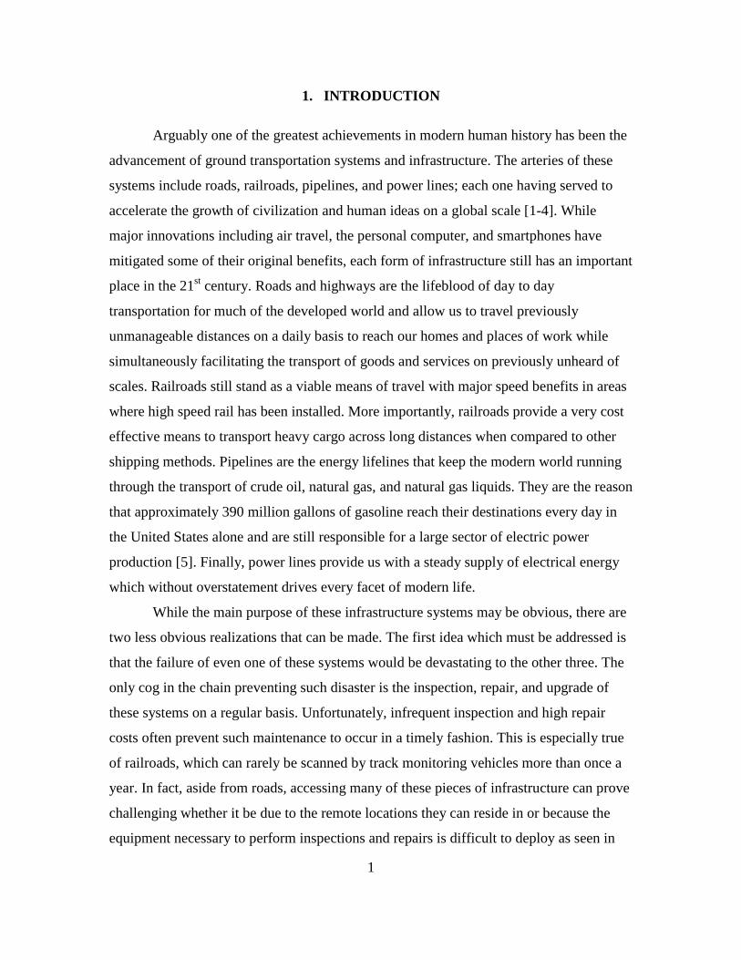
themselves under normal operating conditions, but can be seen in Figure 9 easily under

conditions where the camera is moving [18]. The top-to-bottom image generation

technique of the rolling shutter sensor induces skew as the bottom portions of the image

are shifted from right to left as seen in the skewed sign in the rolling shutter image.

Meanwhile the global shutter preserves the geometry but induces some blur as a result of

the sensors on the CCD reading neighboring values along the pan direction. While both

sensors have appropriate applications, moving UAV applications where computer vision

techniques are being applied are better suited to global shutter cameras as geometry

preservation is the most important factor in most situations. At high frame rates and low

exposure times, global shutter blur effects can almost completely dissipate further

reinforcing the case for global shutter cameras on UAV platforms.

15

Figure 9. Consequences of Rolling and Global Shutters for Moving Cameras

Now the major factors affecting UAV camera and lens selection have been

discussed. However, once the camera has been mounted and images can be collected,

what can we do with that data? The next step is to discuss how computer vision

techniques can be applied to these raw images to extract useful data with the eventual

goal of identifying trajectories for UAVs to follow linear infrastructure.

2.3 Computer Vision Concepts

Computer vision is a vast field capable of extracting an almost infinite amount of

data from images. It can be used for everything from surveillance and robotics to photo

organization and image searching. In the field of UAV navigation, as is the case for this

paper, many of the computer vision concepts that were used relate to fast extraction of

navigational data. A large subset of the algorithms currently available are not applicable

to this task as they could result in navigational failure or even catastrophic crashes.

Therefore, the following low level computer vision concepts were chosen first and

foremost because of the relatively low computational cost they impart compared with

more high level operations. The algorithms discussed later in the paper will all rely on

these fundamental operations. However, before jumping into computer vision itself, it is

first useful to understand digital images.

A digital image can be thought of as a two dimensional matrix, where each

individual position in the matrix corresponds to pixel. In the case of 8 bit images, each of

these pixels has a value ranging from 0 – 255 called the pixel intensity. In a classic

grayscale image as seen in old photography before the advent of color sensors, black

corresponded to the value 0, white corresponded to the value 255, and ever increasingly

16

bright shades of gray ranged in between. With the advent of color, however, the

complexity of the image matrix increased.

2.3.1 Color Spaces

The most popular color space in modern digital imagery is the RGB space

corresponding the colors red, green, and blue. An RGB image can be thought of as three

grayscale images superimposed on top of each other to form one three dimensional RGB

image matrix. The top matrix contains the red intensities in each pixel, the middle matrix

contains the green intensities, and the bottom matrix contains the blue intensities. By

varying how intense each pixel’s RGB values are respectively, most colors can be

generated.

Another popular set of color spaces which derive from RGB are the hue saturation

luminance (HSL), hue saturation value (HSV), and hue saturation intensity (HSI)

systems. To understand these systems as a whole, their individual planes must first be

explained. As these color planes are usually visualized along a cylinder as seen in Figure

10, hue represents the angular dimension of the cylinder and can be thought of as

defining which specific color is being perceived i.e. red, orange, yellow, green, blue,

indigo, and violet. As such, each angle or hue can be considered a different nameable

color. To calculate hue, equations 9 – 12 can be employed which upon inspection show

that hue calculates differently depending on the most prominent RGB color in the pixel.

This is an important factor to consider as hue will not calculate the same way across

different images making it challenging to use in certain computer vision applications.

𝑀 = max(𝑅, 𝐺, 𝐵) (9)

𝑚 = min (𝑅, 𝐺, 𝐵) (10)

𝐶 = 𝑀 − 𝑚 (11)

𝐻 =60°

𝐶 ∙ ({

𝐺 − 𝐵, 𝑖𝑓 𝑀 = 𝑅𝐵 − 𝑅, 𝑖𝑓 𝑀 = 𝐺𝑅 − 𝐺, 𝑖𝑓 𝑀 = 𝐵

) , 𝑒𝑙𝑠𝑒 𝑢𝑛𝑑𝑒𝑓𝑖𝑛𝑒𝑑 (12)

One thing hue does not indicate is how much of that named color is present. Enter

saturation, the radial dimension of the cylinder which defines the depth and richness of

the color. One useful way to think of saturation is to refer back to the RGB space, where

17

each plane’s pixel intensity corresponded to how much red, green, and blue was present.

Saturation works much the same way, but each plane is now represented by a different

hue angle instead of just red, green, and blue. It should be noted that saturation is

calculated differently in the color spaces mentioned because of the subtle differences

between luminance, value, and intensity. The equations governing these three saturation

calculations are provided in equations 13 – 15.

𝑆𝐻𝑆𝐿 = 𝐶

1−|2𝐿−1| (13)

𝑆𝐻𝑆𝑉 = 𝐶

𝑉 (14)

𝑆𝐻𝑆𝐼 = {0, 𝑖𝑓 𝐶 = 0

1 − 𝑚

𝐼, 𝑜𝑡ℎ𝑒𝑟𝑤𝑖𝑠𝑒

(15)

Finally comes the vertical height dimension of the cylinder represented by

luminance, value, or intensity. While easiest to visualize in Figure 10 as lightness,

luminance defines the whiteness of a color is with comparison to true white. This is very

different from value, which can be thought of as how much black is in a color with

respect to its most rich and bright form. Probably the most difficult to visualize and thus

not depicted plane of these color systems is intensity. Often defined as the amount of

light passing through a color, it is less ambiguous to simply declare it as the average of

the red, green, and blue values in the RGB system. In this way, it can be understood more

clearly as how much total color is present. The calculations for these three planes is

shown in equations 16 – 18 [19].

𝐿 = 𝑀+𝑚

2 (16)

𝑉 = 𝑀 (17)

𝐼 = 𝑅+𝐺+𝐵

3 (18)

18

Figure 10. HSL and HSV Color Space Cylindrical Models - Diagram showing the

HSL color space (left) and HSV color space (right).

The final color system which must be understood for this paper is the Lab color

space in the spherical system shown in Figure 11. Although its equations of derivation

are quite in depth and are beyond the scope of this thesis, it was still used because of its

unique nonlinear transform that seeks to separate all colors evenly. This is important with

regards to computer vision and more specifically color classification because it

guarantees linear distance between colors. As for the planes in the Lab system, L

corresponds to the brightness and like luminance determines how much white is present

in the color. The a plane contains red and green values where all red values are positive

and all green values are negative. The b plane works the same way but with positive

yellow values and negative blue ones [20].

Figure 11. Lab Color Space Spherical Model

The reason all of these color planes exist in the first place is that they have

advantages in different applications and better extract information in different image

situations. For this reason, combining information from these different color spaces

enhances computer vision applications such as classification more than just using one

19

color model at a time. The main advantage of using color is that it computes very quickly

since the data is a direct derivative of the raw data coming from the camera. However,

color cannot provide all of the information necessary to accomplish most meaningful

computer vision tasks.

2.3.2 Filters, Edges, and Texture

Sometimes it is useful to alter the default pixel values that reside in images by

relating each pixel value to its neighboring pixel values. In the field of computer vision,

this is often done through the use of filters. Filters are small matrices which, when slid

across the pixels in an image, produce some new image with a desired result. Filters can

do everything from blur pixels together through neighborhood averaging to sharpening

fine details. These different operations are achieved by altering the filter matrix values,

size, or by using mathematical combinations of filters together. It is important to note that

filters generally only work on two-dimensional or grayscale images. Therefore, one must

select a particular color plane (usually luminance) to serve as the image to be filtered.

That said, three dimensional filters due exist for filtering RGB and other 3D color spaces.

Some examples of common filter matrices can be seen in Figure 12 [21].

Figure 12. Examples of Common Computer Vision Filters - The averaging filter (left)

works by summing the multiples of 1 and a 3x3 neighborhood around the central pixel

together and dividing by 9 to generate and average image. The sharpening filter (middle)

creates one image that has double the pixel values and subtracts the average image to

generate an image with sharp edges. The median filter (right) is a nonlinear filter that

calculates the 3x3 median of window around each pixel to generate an image with

reduced noise.

One common application of filters in computer vision is to enhance the edges of

objects. Often called edge detection, the goal of this process is to produce an image

where the edges of the image have a higher pixel intensity (closer to white) than the

smoother more uniform regions of the image. An edge can be considered any location in

20

an image where the pixel value changes abruptly from one value to another. To detect

such pixel changes using a filter, generally the filter design must be capable of extracting

the pixel differences in a neighborhood around the pixel of interest to determine how

alike that pixel is to its surroundings. While there are many popular edge detection

algorithms including Canny, Prewitt, Roberts, and even custom machine learning

designs, the one employed in this thesis was the Sobel edge detector [22]. Sobel has the

advantage of producing stronger horizontal and vertical edges than Prewitt or Roberts

while providing angle information and general edge magnitude information that Canny

cannot. Canny does provide sharper and more defined edges than Sobel, but its added

computational cost and the fact that it converts the image to binary made it a non-useful

candidate for this work [23]. The XY Sobel filter matrix and representative equation are

shown in Figure 13 and equation 19 below.

Figure 13. XY Sobel Filter - Given the input image of a road (left), convolving with the

XY Sobel filter (middle) produces the Sobel edge image (right)

𝑃𝑖𝑥𝑒𝑙 𝑉𝑎𝑙𝑢𝑒 = √[−(𝑟 − 1, 𝑐 − 1) − 2(𝑟, 𝑐 − 1) − (𝑟 + 1, 𝑐 − 1) + (𝑟 − 1, 𝑐 + 1) + 2(𝑟, 𝑐 + 1) + (𝑟 + 1, 𝑐 + 1)]2

+[−(𝑟 − 1, 𝑐 − 1) − 2(𝑟 − 1, 𝑐) − (𝑟 − 1, 𝑐 + 1) + (𝑟 + 1, 𝑐 − 1) + 2(𝑟 + 1, 𝑐) + (𝑟 + 1, 𝑐 + 1)]2

(19)

Another major use of filters in computer vision is to get a sense for the texture

within in an image. Filters designed for this application often seek to gather statistical

data about their surroundings and apply these statistical results to the pixels they are

filtering. One can imagine for example gathering statistical data about the number of

edges in a given neighborhood to approximate the roughness texture of the object.

Common examples include standard deviation filters, histogram filters, and even shape

filters where a filter approximating the shape of a repeating pattern in an image tries to

locate such patterns by giving off a high response in those areas [24]. One texture filter

used in this work was called the entropy filter. Similar in application to the median filter

in Figure 12, the entropy filter works by applying the local entropy of the filter

21

neighborhood to the pixel of interest in a grayscale image. Entropy is referred to as the

randomness of an image section and can be thought of as the variation in contrast and

pixel value. The formula for entropy is shown in equations 20 – 21 [25-27].

𝑝 = 𝑟𝑒𝑚𝑜𝑣𝑒 𝑧𝑒𝑟𝑜 𝑒𝑙𝑒𝑚𝑒𝑛𝑡𝑠 ([ℎ𝑖𝑠𝑡𝑜𝑔𝑟𝑎𝑚(𝑛𝑒𝑖𝑔ℎ𝑏𝑜𝑟ℎ𝑜𝑜𝑑 𝑝𝑖𝑥𝑒𝑙 𝑣𝑎𝑙𝑢𝑒𝑠)

𝑛𝑢𝑚𝑏𝑒𝑟 𝑜𝑓 𝑛𝑒𝑖𝑔ℎ𝑏𝑜𝑟ℎ𝑜𝑜𝑑 𝑝𝑖𝑥𝑒𝑙𝑠]) (20)

𝐸 = − ∑ 𝑝𝑖 log2 𝑝𝑖𝑠𝑖𝑧𝑒(𝑝)𝑖=0 (21)

The techniques mentioned up to this point have been useful for extracting

information from color and grayscale images, but there are situations where altering or

collecting data from specific objects in an image can be useful. To do this, techniques

exist to work on a specific image type called binary.

2.3.3 Binary Operations

A binary image is any image which has only two pixel values, usually 0 and 1.

Binary images are useful because they allow separate features or objects in an image to

be modified or analyzed simply by running algorithms which detect the presence of 0s

and 1s in a region. One of the most common techniques to generate a binary image is to

threshold the image. Thresholding is a process where a user or user defined algorithm

specifies a pixel value to serve as the threshold point. Any value below the threshold

becomes a 0 and any values equal to or above the threshold become a 1. This technique

can be extrapolated using two threshold values to specify a “bandpass” type threshold

where values outside the window are 0 and values inside the window become 1. This is

especially useful when thresholding color images where a specific range of RGB values

is desired so that a specific color can be extracted from the image. Aside from

thresholding, another main way that binary images can be generated is via machine

learning classification. In this scenario, a machine learning algorithm has been trained to

label pixels or pixel regions as 0 or 1 based on a complex set of features it has learned.

This technique can yield much more predictable results and was the technique mostly

employed in this work. While generating the binary image is important, modifying and

extracting data from it is where things get interesting. A complete list of the low level

binary morphological operations and data parameters used is presented below:

22

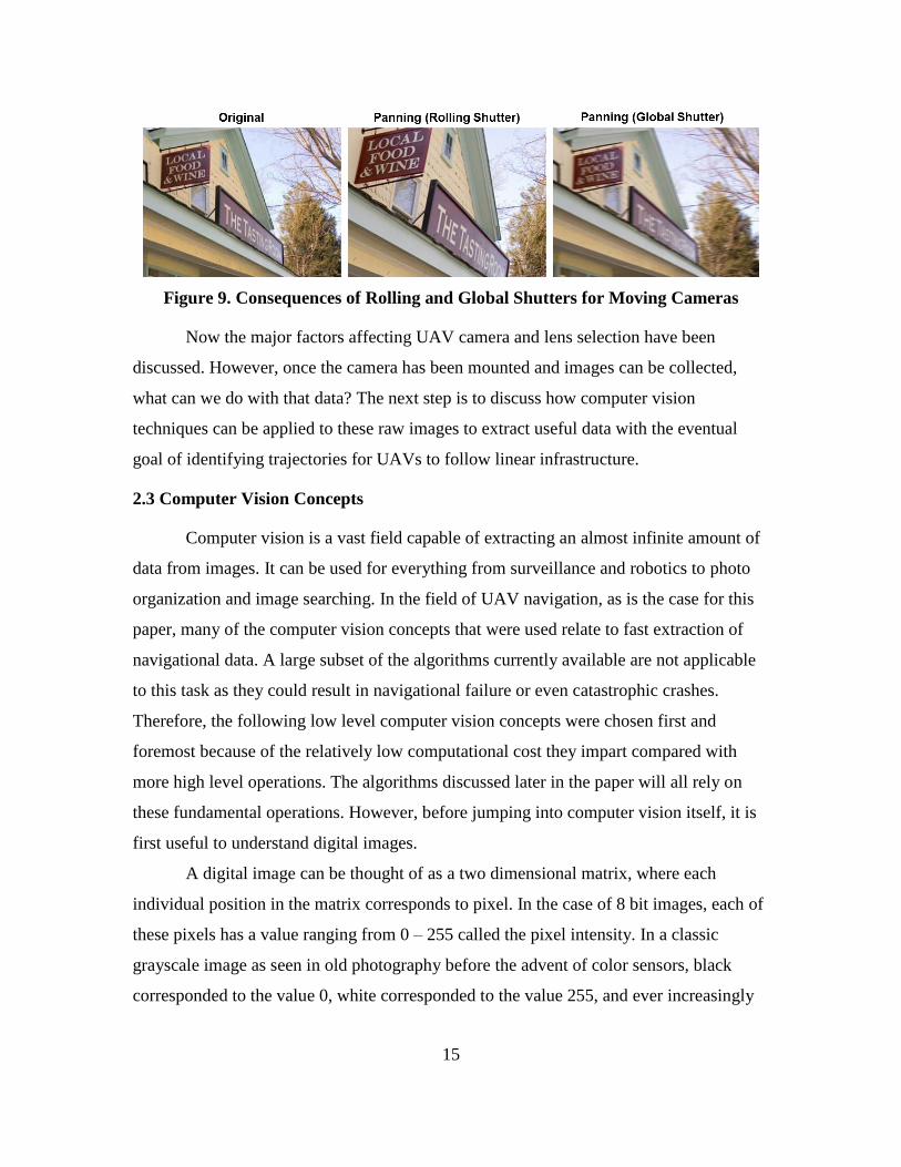
1 Inverse – The inverse of a binary image is an image where all pixel values are

opposite their original value i.e. 0 becomes 1, 1 becomes 0. To calculate the

inverse, equation 22 can be employed.

𝑖𝑛𝑣𝑒𝑟𝑠𝑒 = 𝑋𝑂𝑅(𝑏𝑖𝑛𝑎𝑟𝑦 𝑖𝑚𝑎𝑔𝑒, 1) (22)

2 Dilation – This operation refers to the process of increasing the size of foreground

objects in a binary images. A foreground object can be considered a pixel or a

connected group of pixels all sharing the value 1. The algorithm begins by sliding

a structuring element (similar to the filters described before) across the pixels in

the binary image. A structuring element or 𝑆𝐸 is a matrix where all elements

which are to be analyzed have values of 1 and all elements to be ignored have

values of 0. By organizing the placement of 1s and 0s in the structuring element,

various element shapes can be generated to produce different results. In the case

of dilation, all of the elements in the sliding structuring element labeled 1 have the

algorithm in equation 23 applied to the pixel located at the center of the

structuring element. In this way, the value 1 is padded around all foreground

objects in the image with depth equal to the size of the structuring element.

𝑐𝑒𝑛𝑡𝑒𝑟 𝑝𝑖𝑥𝑒𝑙 𝑣𝑎𝑙𝑢𝑒 = {𝑐𝑢𝑟𝑟𝑒𝑛𝑡 𝑣𝑎𝑙𝑢𝑒, 𝑆𝐸(1) = 0

1, 𝑆𝐸(1) = 1 (23)

3 Erosion – Identical to the dilation algorithm except, as seen in equation 24,

foreground objects are reduced in size as their pixels values are set to 0.

𝑐𝑒𝑛𝑡𝑒𝑟 𝑝𝑖𝑥𝑒𝑙 𝑣𝑎𝑙𝑢𝑒 = {𝑐𝑢𝑟𝑟𝑒𝑛𝑡 𝑣𝑎𝑙𝑢𝑒, 𝑆𝐸(1) = 1

0, 𝑆𝐸(1) = 0 (24)

4 Opening – Referring to an erosion followed by a dilation, this technique is useful

for removing small objects from an image while still preserving the shape of the

main foreground objects. Imagine eroding a binary image until all of the small

foreground objects are removed. Since they are gone, they will not reappear when

dilated. However, the objects that remain can return to their original shape once

they have been dilated the same number of times that they were eroded.

5 Closing – Referring to a dilation followed by an erosion, this technique is useful

for filling holes in objects while preserving the original shape of the external

objects. A hole is defined as a 0 valued pixel or set of connected pixels that is

23

surrounded by foreground pixels. Therefore, subsequent dilations can be used to

keep replacing these 0 values until the hole is filled. Following this operation by

an identical number of erosions will return the main foreground object back to its

original size and assuming the hole was completely removed in the dilation phase,

will not cause the hole to reappear.

6 Skeleton – The skeleton of a binary object is similar to the internal skeleton of an

organism in that it forms the structure of the objects shape. Binary skeleton

algorithms strive to remove the most amount of foreground pixels from the object

of interest as possible while still retaining a single pixel wide line which

represents the overall object’s shape. Many algorithms have been developed that

generate such skeletons, but the specific algorithm used in this paper was

developed by Lantuéjoul [28]. Also called morphological skeletons, the skeletons

produced by Lantuéjoul's algorithm are generated via repetitive conditional

opening and thinning operations which run until the entire skeleton is only one

pixel in width. The specific algorithm is a paper in itself and thus will not be fully

discussed in this document. However, the reason this algorithm was used over

other implementations such as M-skeleton is that the Lantuéjoul skeleton (L-

skeleton) produces far less branches or deviations from the true object shape

while still maintaining a reasonable execution time [29].

7 Region Properties –

a. Number of Objects – This parameter refers to the number of foreground

objects in a binary image or the number of unique connected sections of

pixels with the value 1. To calculate this, an algorithm is generally

implemented called the two pass algorithm. This algorithm works by first

scanning through each pixel in the image with a 3x3 cross shaped

structuring element. The first foreground pixel the element passes over is

labeled 1. If the structuring element is hovering over this foreground pixel

when it reaches the next foreground pixel, that pixel is labeled 1 as well.

Otherwise, the next foreground pixel is labeled 2. This continues in a

cumulative fashion until pass one is complete. On pass two, all of the

numbered pixels are scanned through to determine if they are touching any

24

pixels with different numbers. Upon finding this situation, all pixels that

were set to a higher number value are reset to the lower value. When this

algorithm is finished, each binary foreground object will have its own

pixel value. The max pixel value therefore will be the total number of

foreground objects in the image [30].

b. Number of Holes – This algorithm can only be implemented upon

completing the number of objects procedure. Next, the locations of each

foreground object are stored, the pixels surrounding each border object are

stored, and a new image is created that is the inverse of this binary image.

By running the number of objects algorithm along the pixels making up

each object in the image, the total number of binary pixels that could be

holes can be found. Then by removing any candidates with pixels shared

by the outer border of the foreground object, the total number of holes can

be calculated [31].

c. Area – This refers to the number of pixels making up a connected set of

foreground pixels. Upon completing the number of objects analysis, this

can be calculated by summing the total number of elements with an equal

pixel value.

Using a combination of these low level operations, a wide array of problems can

be solved including a large portion of the filtering and data extraction presented in the

road following algorithm later in this paper. That said, the previously mentioned

algorithms have all been fairly low level. Some of the main computer vision tools for

detecting specific shapes and objects in an image require more complex strategies to

work effectively as will be seen in the following sections.

2.3.4 Hough Transform

Many objects in the real world can be approximated by or are made up of simple

shapes which can make their identification process much easier. One of the most basic

shapes that exists is a straight line. As is the case for all shapes in an image, they can be

approximated as 2D even if the real world object the camera was trying to capture was

3D. But how would one go about detecting a simple 2D shape in an image, even one as

25

basic as a straight line? For starters, it is helpful to think of a line as a collection of points

that lie along the algebraic function shown in equation 25 below.

𝑦 = 𝑚𝑥 + 𝑏 (25)

An algorithm which was capable of finding high responses to the line equation at

different slope and intercept values would be a good starting place. However, this is

difficult to iterate through effectively in the classic XY space that images reside in. Enter

the Hough transform, an algorithm which transforms data from the image space to a

voting space by changing the XY axes to parameters of the shape equation that is trying

to be fit. In the case of line fitting, the Hough transform changes the default space with

horizontal x-axis and vertical y-axis to a voting space with horizontal slope-axis and

vertical intercept-axis. Therefore, the Hough equation for a line changes to the form

shown in equation 26.

𝑏 = 𝑥𝑚 − 𝑦 (26)

The idea of the Hough transform is simple. As more and more points are

transformed to the voting space, popular slopes and intercepts will begin to overlap each

other producing large accumulations of points. At the end, the most popular slopes and

intercepts can be extracted and returned to the XY space thus indicating the best line

candidates in the original image. However, some red flags should already be presenting

themselves. For starters, although the XY shape points are provided in the original image,

usually from running an edge detection algorithm to extract shape borders, the only way

to iterate through all possible slope and y-intercept values in the image is to loop through

all possible values of slope and intercept. This presents an issue as vertical lines can exist,

but in the slope world they cannot be represented since they result in the generation of an

undefined slope value. Luckily, there exists another form of the line equation which

works at all angles. This form, shown in equation 27, is called the polar line equation and

replaces the Hough terms for slope and y-intercept with two new terms with 𝜃

representing the angle of the line with respect to horizontal axis and 𝑑 representing the

orthogonal distance from the line to the origin.

𝑑 = 𝑥 cos 𝜃 − 𝑦 sin 𝜃 (27)

26

However, there is still the issue of looping through all possible angles in the

Hough space which adds a lot of computational complexity. Even when specifying

discrete windows of values to loop through, the nested for loops required to run the

Hough transform in this fashion slow down the overall program functionality immensely.

Luckily, the XY Sobel filter described earlier can be used to output the specific angle to

check at each edge point thus reducing the Hough transform to only looping through all

edges rather than all edges and all angles. The equation for extracting the angle value for

a given edge in the XY Sobel filter is seen in equation 28.

𝜃 = tan−1 (𝑆𝑜𝑏𝑒𝑙 𝑌 𝑅𝑒𝑠𝑝𝑜𝑛𝑠𝑒

𝑆𝑜𝑏𝑒𝑙 𝑋 𝑅𝑒𝑠𝑝𝑜𝑛𝑠𝑒) (28)

With the Hough transform for lines now simplified computationally and able to

detect lines at all angles, the voting procedure can begin. As seen in Figure 14, the Hough

space resembles a grayscale image when visualized in image form. Higher pixel values or

bin counts correspond to line equations that were selected more often during the voting

process. This happens because each 𝜃 and 𝑑 value that is calculated in the Hough space

causes a vote of +1 pixel value to appear in that location. Therefore, the top line

candidate corresponds to the point of maximum intensity in the Hough space. This can be

extrapolated further to detect N multiple lines if the top N maxima in the Hough space are

used to generate line equations. Once these equations are overlain on top of the original

image, the Hough transform is complete and the detected lines can be used as meaningful

output data [32].

Figure 14. Summary of Hough Transform for Line Detection

27

2.3.5 Color Pattern Matching

While detecting shapes provides a wide variety of image information, it does not

work well for detecting complex objects in images. To do this, a technique called color

pattern matching must be employed. As seen in Figure 15, color pattern matching is the

process of comparing stored data from a template image with data in a new image to find

similar features or objects. This can be useful for a lot of applications including object

detection, image alignment, and image scaling. The two techniques that combine together

to form the color pattern matching algorithm are normal color matching followed by

grayscale template matching [33].

Figure 15. Goal of Color Pattern Matching

In the color matching step, the color distribution of the template image is

extracted and stored in an Nx3 vector, where the columns represent the RGB channels

and the rows represent the number of pixels in the template. The template is then

normalized so that all the values lie between 0 and 1 through column independent

maxima division. This same process is then completed with a scaled down version of the

template. With the scaled down color vector generated, new color vectors extracted from

a scaled down input image are compared against it by calculating their Mahalanobis

distances between each other. This scaled down comparison yields the most likely

candidate locations for matches in the full sized image while rapidly reducing the

computational expense of a full size image search. With the candidate locations found,

the full sized template regions in the image are compared to the full size template color

28

vector. The smallest distances are then considered the best color matches in the image.

However, the color match technique does not produce accurate pattern matching results

on its own since regions of an image could have similar overall color while representing a

completely different object. This is where the grayscale template matching step comes in.

It begins by converting candidate regions from the color matching portion of the

algorithm into grayscale images via the RGB conversion in equation 29 [34, 35].

𝑔𝑟𝑎𝑦𝑠𝑐𝑎𝑙𝑒 𝑣𝑎𝑙𝑢𝑒 = 0.21𝑅 + 0.72𝐺 + 0.07𝐵 (29)

Next, a Sobel edge detector is used to extract edge information from the grayscale

regions to be used as features for matching the template to. After thresholding the edge

image so that only edges of a desired strength remain, the remaining edges are added to

an Nx1 feature vector which counts the number of edges in each section of the N sections

of the region being scanned. This vector is then compared with the same vector generated

from the template image using the same distance scoring technique, where lower

distances equal better scores. Finally, the highest score match from this technique is set to

the best color pattern matching candidate. One detail left out however is how scale and

rotation invariance is handled in this technique. For scale invariance, a Gaussian pyramid

of various downscaled version of the template and scan locations are formed. By

analyzing the lowest resolution data first, computational time can be reduced and

templates of smaller sizes can be found. For rotation invariance, the same bottom-up

approach is used where rotated versions of the smallest template are compared with the

input vector from the image to detect matches at different angles [36].

With the conclusion of this section, a general understanding of the underlying

computer vision principles and algorithms used in the advanced algorithms later in this

paper should be attained. One aspect of computer vision introduced in this section which

was novel compared to the other methods mentioned was the idea of matching previously

stored data in the form of templates with newly collected data. This technique comes

from another major subject field utilized in this thesis called machine learning.

‘

29

2.4 Machine Learning Algorithms

Machine learning is defined as the “field of study that gives computers the ability

to learn without being explicitly programmed [37].” Using a vast array of complex

algorithms for finding meaning in data, machine learning can solve problems and find

patterns that humans would struggle with or find impossible. The power of machine

learning has an almost infinite number of applications, but a few include mining medical

data to find trends indicating disease causes or potential cures, monitoring of user

accounts on websites to correlate past purchases and likes with possible future products

of interest, or the analysis of human speech and writing to generate more accurate voice-

recognition software. At its core, all machine learning algorithms rely on collecting data

in the form of features. Features can literally represent anything, but all features must be

capable of conversion to numerical data. While this conversion is built in for quantitative

data, other data situations might not be obvious to translate. For example, true-false

questions might have answer features represented as 0 or 1. The goal of a machine

learning algorithm is then to make use of these features by either clustering them into

groups based on statistical similarity, separating them into classes based on past feature

examples that were labeled by humans, or making decisions based on the overall trend

found in the data. This leads to two main categories of machine learning approaches,

unsupervised and supervised learning.

2.4.1 Unsupervised Learning

Unsupervised learning is the branch of machine learning associated with making

decisions about data without any prior labeled examples from humans. This means that

the computer must make all of its decisions about how to organize the data and what

meaning should be drawn from it strictly using the data provided. In computer vision

applications, unsupervised techniques can be used to cluster image pixels together into

groups based on a variety of features such as their color, texture, edge responses, etc. One

such algorithm used in this work was kMeans clustering.

KMeans is a simple and fast clustering algorithm compared to other unsupervised

techniques that nonetheless works well for a wide variety of applications. The main

caveat is this algorithm requires that the number of clusters desired is known ahead of

30

time. As seen in Figure 16, kMeans begins by initializing k number of cluster centers in

the feature space. Next, the distances between each feature in the feature space and the

cluster centers is calculated to determine which cluster center is nearest by each feature.

Each feature is then given the label of its nearest cluster center and all features with the

same label are averaged together to generate a new cluster center value. When this step

completes for all clusters, the cycle repeats until the average values at the end are equal,

within some error bounds, to the current cluster center.

Figure 16. Flow of kMeans Algorithm

As one might ascertain from this description, the placement of initial cluster

centers is vital to getting good results. While this can lead to undesirable clustering

results when random cluster centers are chosen, guiding the cluster center initialization

points by maximizing separation or using expert knowledge about the problem at hand

can mitigate the issue [38]. Unsupervised techniques works well when the feature output

cannot be predicted ahead of time, but supervised learning techniques are arguably more

useful for obtaining definite results.

31

2.4.2 Supervised Learning

Supervised learning is the more conventional form of machine learning where

prior examples influence the decisions of the algorithm. Given a group of human-labeled

training feature sets, a supervised machine learning algorithm will compare the new test

feature sets against them to figure out which training features most resemble the new

data. Computer vision can utilize this in a number of ways including scene classification,

face detection, and template matching as discussed earlier. The two supervised machine

learning algorithms used during my work were k-nearest neighbors (kNN) and support

vector machine (SVM).

The kNN algorithm is perhaps the most basic supervised machine learning

algorithm available. That said, it has the advantage of being easy to implement, inherent

multiclass support, and overall strong performance with enough training examples. The

first step in any supervised learning algorithm, with kNN being no exception, is to build

the training set with labeled features. This involves a user collecting data from prior

examples of their problem of interest and assigning features extracted from the data to

particular classes. It is important that the feature space becomes sufficiently large or

representative enough of the overall distribution of likely feature outcomes. In most

supervised learning techniques, the next step would be to train the algorithm on the

feature space to learn the decision boundary between the different labeled regions. In the

case of kNN, the training step is inherent and thus the main implementation can begin

immediately. Given a new feature sample, kNN will calculate the distance between this

feature sample and all of the feature samples in the training set. While many different

distance functions can be used including Euclidian, SSD, and Mahalanobis, the best k

matches will be the distances with the smallest values. Out of the k best matches, the

most common label amongst them will become label of the new feature [39].

One of the weaknesses of kNN is that its execution time will increase as function

of the number of features in the training set since the distance between each labeled

feature and the new feature must be computed. Although matrix operation distance

calculations can drastically reduce this time, one of the best techniques for calculating

distances in large training sets is to use representative cluster centers, like those obtained

32

from kMeans, as index queues first. By calculating the distances between the cluster

centers first, a general feature match location can be narrowed down thus drastically

improving execution time [40]. While kNN is very useful in many situations, other more

complex algorithms like SVMs can generally produce higher classification accuracies.

SVMs have been heavily used in machine learning applications since the mid-

2000s and have consistently proven themselves as the go to supervised learning algorithm

for most basic applications before implementing more time consuming techniques such

as neural networks. This is because through the use of a wide variety of tunable

parameters and kernel functions, SVMs can take many forms to fit different feature set

layouts. The overall idea of an SVM, as seen in Figure 17, is to separate two training

classes of data by the maximum possible margin [41]. But how is this actually

accomplished mathematically [42, 43]?

Figure 17. Support Vector Machine Basics - Given two training sets with classes (1)

and (2) in which it is desired to generate a function which distinguishes between them, an

SVM can find the support vectors (3) in the training set which separate the two classes

from each other along a central hyperplane (4) at a maximum distance or margin (5)

To start, let us consider the default 2D linear SVM which tries to separate a 2D

feature space with two classes by a hyperplane represented as a line. Referring to

equation 25, the equation of a line can be rewritten to the form shown in equation 30 after

introducing an additional scalar constant 𝑐 to the 𝑦 term. We then introduce two new

variable vectors 𝒘 and 𝒙 to simplify future operations as seen in equation 31.

𝑚𝑥 + 𝑐𝑦 + 𝑏 = 0 (30)

33

𝒘𝒙 + 𝑏 = 0 𝑤ℎ𝑒𝑟𝑒 𝒘 = [𝑚𝑐

] 𝑎𝑛𝑑 𝒙 = [𝑥𝑦] (31)

The next step is to find a way to calculate the distance from this hyperplane line to

any point in the 2D feature space. Using the newly defined terms in equation 31, this

distance term can be calculated using the formula shown in equation 32. It turns out that

support vectors, the features with the smallest distance 𝐷 from the hyperplane, should

meet the criteria in equation 33, with class label one being equal to +1 and class label two

being equal to -1. Therefore, any class label for either class one or two should meet the

criteria in equation 34. This results in the desired 𝐷 for a support vector in equation 35

which can also be visualized as twice the maximum margin (5) in Figure 17.

𝐷 = 𝒘𝒙+𝑏

‖𝒘‖ (32)

𝒘𝒙 + 𝑏 = ±1 (33)

𝒘𝒙 + 𝑏 ≥ 1 𝑓𝑜𝑟 𝑐𝑙𝑎𝑠𝑠 𝑜𝑛𝑒, 𝒘𝒙 + 𝑏 ≤ −1 𝑓𝑜𝑟 𝑐𝑙𝑎𝑠𝑠 𝑡𝑤𝑜 (34)

𝐷𝑠𝑢𝑝𝑝𝑜𝑟𝑡 𝑣𝑒𝑐𝑡𝑜𝑟 = (1−(−1))

‖𝒘‖=

2

‖𝒘‖ (35)

The main takeaway from the equations shown thus far is that we want to maintain

the class labeling criteria in equation 34 so that all feature vectors are labeled while

maximizing equation 35 which represents the margin between them. It turns out that the

problem that finds these solutions is a quadratic optimization problem with the final

solution shown in equation 36, where 𝑎𝑖 represents the weight of support vector 𝑖, 𝑦𝑖 is

the class association of that support vector (-1 or +1), 𝒙𝒊 is the support vector 𝑖, 𝒙 is the

unknown vector in which classification is desired, and 𝑏 is now equal to the distance

from the hyperplane to the origin. This can then be rewritten as the classification function

in equation 37 since can 𝑦𝑖 be handled by the sign operation.

𝒘𝒙 + 𝑏 = ∑ 𝑎𝑖𝑦𝑖𝒙𝒊𝒙 + 𝑏𝑖 (36)

𝑙𝑎𝑏𝑒𝑙 = 𝑠𝑖𝑔𝑛(∑ 𝑎𝑖𝒙𝒊𝒙 + 𝑏)𝑖 (37)

In the case of linear SVMs, equation 37 is the final form of the function necessary

to classify two class data. But what about data that is not linearly separable? In this case,

an SVM technique called the kernel trick must be implemented to transform the default

34

feature space into some higher dimensional space related to the kernel choice. A kernel is

simply a function of 𝒙𝒊 and 𝒙 that, upon calculation, ideally transforms the default

classification into a more separable form. The classification equation for SVMs using the

kernel trick is seen in equation 38 below.

𝑙𝑎𝑏𝑒𝑙 = 𝑠𝑖𝑔𝑛(∑ 𝑎𝑖𝐾(𝒙𝒊, 𝒙) + 𝑏)𝑖 (38)

One such kernel used in this work was the Gaussian or RBF kernel. Seen in

equation 39, the Gaussian kernel is an implementation of the Gaussian distribution

around the support vector. The logic behind this function is that by adjusting the standard

deviation term, new vectors nearby the support vector can receive higher values the

closer they are to the support vector. This is useful for datasets in which the support

vectors for the two different classes have small margins between them. Feature vectors

that would normally have high scores for both support vector classes will now be heavily

weighted to the support vector that they are the nearest to rather than having very similar

values for both.

𝐾(𝑥𝑖, 𝑥) = exp (−‖𝒙𝒊− 𝒙‖2

2𝜎2 ) (39)

Another point worth mentioning with regards to support vector machines is how

to classify data with more than two class labels. Inherently, SVMs can only generate

hyperplanes between two labeled datasets at a time. Therefore, in order to actually

separate multiclass data, multiple two class SVMs must be trained independently with the

results from each combined together at the end to generate the final class label for the test

feature points [44].

With the conclusion of this section, enough background should be provided to

facilitate an understanding of the linear infrastructure detection algorithms presented in

the following sections. While railroad detection was the first algorithm developed during

my thesis work, the road detection algorithm will be presented first since it made up a

larger portion of my work and thus its implementation was more complete.

35

3. ROAD DETECTION

The development of a computer vision algorithm to follow roads from the

perspective of a UAV will be outlined in the journal paper excerpt appended in the

following section of this document. However, many aspects of the work that was

accomplished are not encapsulated in the journal itself and thus are presented in the

additional work section that follows. The first of these additional items was the

development of a low level kNN algorithm meant for low resource FPGA

implementation. Next the specific camera selection process that took into account the

needs of this project will be explained. The next section will discuss the custom ground

station software that was developed to control the algorithm in flight. Finally, the

qualitative results that visually show the detection capabilities of the algorithm along with

quantitative results from an HIL simulation of the algorithm will complete the section.

36

3.1 Road Detection and UAV Trajectory Development Algorithm

3.1.1 Road Segmentation

The first step in following any linear feature is to determine where the linear

feature is. In computer vision, there are many techniques for localizing objects of interest

including template matching, feature matching, and segmentation [45]. In the case of

road detection, segmentation is the best approach as it does not require prior knowledge

of the shape, orientation, or scale of the road to make a detection. These are important

criteria to meet as an ideal algorithm for UAV control should be invariant to changes in

altitude and attitude. To perform segmentation, a variety of machine learning techniques

can be employed. Most of these fall within two unique classes, supervised and

unsupervised learning. Supervised learning algorithms base their decisions on prior

knowledge whereas unsupervised learning algorithms use statistical properties within the

data they are given to separate it into meaningful groups. Given that training data could

be collected to quantitatively describe what roads look like and that supervised learning

algorithms generally run more quickly and accurately than unsupervised algorithms,

supervised learning was the best choice to perform this segmentation.

One of the most difficult aspects of developing an efficient and accurate

supervised classification algorithm is feature selection. The key to feature selection is to

minimize the total number and complexity of features while still maintaining a high level

of accuracy and plasticity. In this case, plasticity is the effectiveness of the algorithm at

correctly classifying previously unseen data. To perform road segmentation in real time

onboard a UAV, selecting features which can be calculated very quickly using embedded

hardware was a major requirement. Therefore, it was initially decided to only use features

which were directly captured by the camera (i.e. red, green, and blue pixel values) or

transformations of these values into different color spaces. These additional color planes

included hue, saturation, luminance, value, intensity, and the three CIE L*a*b channels

[46].

To collect these features, 62 images were taken of rural roads with varying

background features including grass, trees, dirt, buildings, and hay bales. Next, a labeled

version of each image was generated manually using Adobe Photoshop. The regions in

37

each image which were deemed to be road pixels were marked as white while all other

pixels were replaced with black values as seen in Figure 18. With a set of labeled images

developed, the next step was to extract features from these labeled regions. Since

LabVIEW was the language the embedded platform (i.e. the NI myRIO) would run on, it

was important to make sure that any collected features were generated using LabVIEW.

This is important because various color transformations like hue are not calculated

consistently between different platforms. Using LabVIEW, 570,382 pixels were extracted

from road labeled regions and 3,865,915 pixels were extracted from the nonroad labeled

regions of the image dataset. For each of these pixels, the eleven previously mentioned

color channel values were recorded into a feature vector as a possible list of features

useful for distinguishing between the road and nonroad pixels. Using Matlab, feature

vectors with less than 2.55% difference between individual features were removed from

the dataset. By removing these relatively redundant values, the calculated percent of

correctly classified features was improved.

Figure 18. Original and Labeled Road Images

To figure out which of the eleven color spaces made the largest impact on

correctly segmenting the road pixels sequential feature selection was employed. As seen

in Figure 19, sequential feature selection involves starting with the minimum number of

features and working up to the maximum number of features. At each feature iteration, an

error function is used to determine how accurately the labels were classified. The error

function used in this case can be seen in equation 40 below.

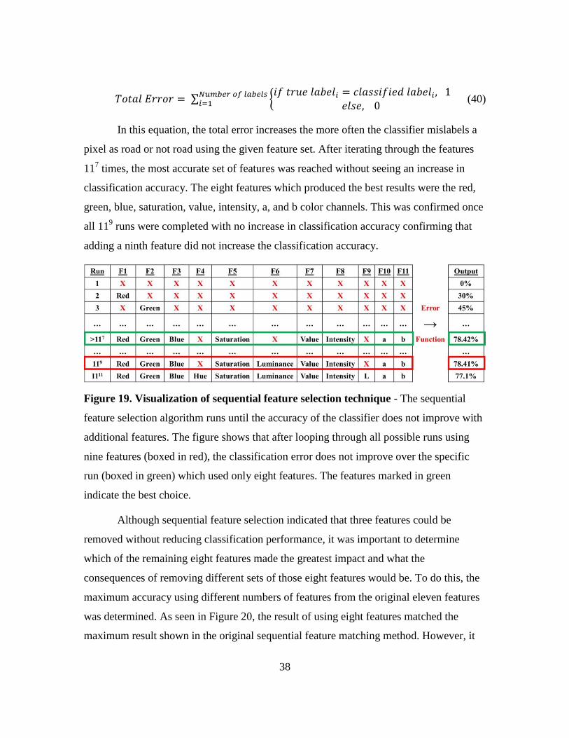
38

𝑇𝑜𝑡𝑎𝑙 𝐸𝑟𝑟𝑜𝑟 = ∑ {𝑖𝑓 𝑡𝑟𝑢𝑒 𝑙𝑎𝑏𝑒𝑙𝑖 = 𝑐𝑙𝑎𝑠𝑠𝑖𝑓𝑖𝑒𝑑 𝑙𝑎𝑏𝑒𝑙𝑖, 1

𝑒𝑙𝑠𝑒, 0 𝑁𝑢𝑚𝑏𝑒𝑟 𝑜𝑓 𝑙𝑎𝑏𝑒𝑙𝑠𝑖=1 (40)

In this equation, the total error increases the more often the classifier mislabels a

pixel as road or not road using the given feature set. After iterating through the features

117 times, the most accurate set of features was reached without seeing an increase in

classification accuracy. The eight features which produced the best results were the red,

green, blue, saturation, value, intensity, a, and b color channels. This was confirmed once

all 119 runs were completed with no increase in classification accuracy confirming that

adding a ninth feature did not increase the classification accuracy.

Figure 19. Visualization of sequential feature selection technique - The sequential

feature selection algorithm runs until the accuracy of the classifier does not improve with

additional features. The figure shows that after looping through all possible runs using

nine features (boxed in red), the classification error does not improve over the specific

run (boxed in green) which used only eight features. The features marked in green

indicate the best choice.

Although sequential feature selection indicated that three features could be

removed without reducing classification performance, it was important to determine

which of the remaining eight features made the greatest impact and what the

consequences of removing different sets of those eight features would be. To do this, the

maximum accuracy using different numbers of features from the original eleven features

was determined. As seen in Figure 20, the result of using eight features matched the

maximum result shown in the original sequential feature matching method. However, it

39

can be shown by the data that beyond using the three features blue, b, and value, there is

not a significant increase in classification accuracy. Therefore, rather than using the

slightly more accurate eight features mentioned before, only these top three features were

used, thus minimizing overall feature space complexity and improving the real time

performance capability of the algorithm.

Figure 20. Down selection of top sequential feature matching features - Although the

maximum classification accuracy occurs when eight features are used, the last major

increase in accuracy (>2%) occurs after only the top three features are used (marked in

green).

While the final three color space features had been identified, the current

classification accuracy of 77.35% with these features did not produce accurate

segmentation results. A new, non-color space based feature would need to be added to

system to improve the segmentation results at the cost of real time performance. This

fourth selected feature, the Sobel edge magnitude, measures the change in pixel value

across pixels in the image along the row and column direction [47]. This response was

40

then smoothed with a 6x6 averaging filter to reduce noise in the edge image. Adding this

feature to the dataset improved the classification accuracy to 94.08% meaning that the

accuracy was now high enough to perform reasonable segmentation.

Several supervised learning techniques were used to segment the road pixels

using these four features including kNN, linear SVM, RBF SVM, and polynomial SVM.

The final technique used which produced the best results was a Gaussian SVM with

s=10. The Gaussian SVM kernel works well in this case because it generates a circular

region of acceptance criteria around the support vectors thus increasing the plasticity of

the algorithm to new inputs. The final segmentation image using the Gaussian SVM

along with a visualization of the features extracted from a test image can be seen in

Figure 21.

Figure 21. Final Segmentation Features and SVM Results - Illustration showing an

input RGB image (top), the four feature planes extracted from it (middle), and the

subsequent segmentation image using those features (bottom)

41

3.1.2 Road Class Detection

With the road pixels separated from the nonroad pixels, the next step was to

determine the number and type of possible routes which could be taken by the UAV. In

general, this meant classifying which type of road junction was present. To do this, it was

first necessary to determine FOV of the UAV camera and thus determine all possible

visible road junctions at the test site within this FOV. The FOV was calculated using

equations 41 and 42.

𝐹𝑂𝑉° = 2(180

𝜋) tan−1 (

𝐶𝑆𝑆

2𝑓) (41)

𝐹𝑂𝑉 = 2𝐴 tan (𝐹𝑂𝑉°

2(

𝜋

180) ) (42)

Using the data in the table in Figure 22, the vertical and horizontal FOV of the

camera was calculated. It was determined that the largest possible road junction within

the field of view the UAV camera at the test site was a four way intersection. Therefore,

it was chosen to limit the scope of the road class detection algorithm development to

detecting a maximum of four way intersections.

Figure 22. Camera Parameters and FOV Visualization (Altitude = 50 m)

Several ideas were originally developed to detect the presence of different types

of road junctions. Corner detection seemed like a reasonable approach since it can be

performed in real time and counting the number of corners along the road would likely

indicate how many possible turns existed. However, most road branches are formed with

gradual curves rather than sharp corners making the approach implausible. The next idea

was to convert the segmented road image into a skeleton image and then to apply a

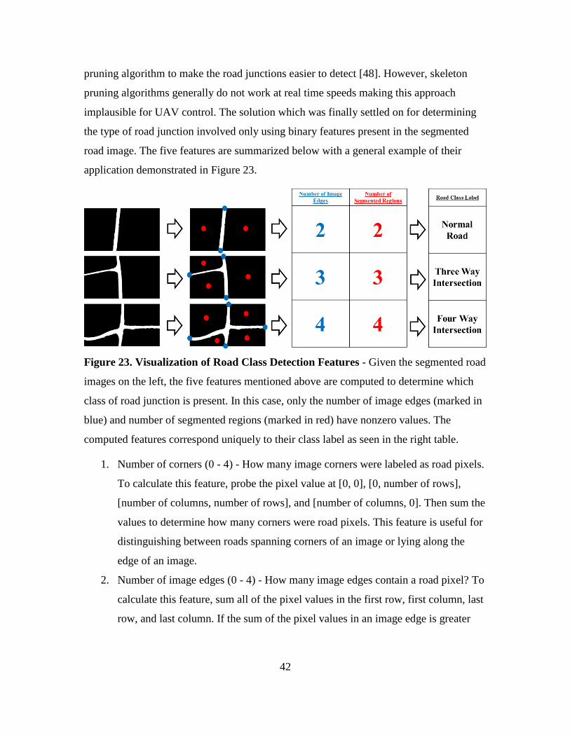
42

pruning algorithm to make the road junctions easier to detect [48]. However, skeleton

pruning algorithms generally do not work at real time speeds making this approach

implausible for UAV control. The solution which was finally settled on for determining

the type of road junction involved only using binary features present in the segmented

road image. The five features are summarized below with a general example of their

application demonstrated in Figure 23.

Figure 23. Visualization of Road Class Detection Features - Given the segmented road

images on the left, the five features mentioned above are computed to determine which

class of road junction is present. In this case, only the number of image edges (marked in

blue) and number of segmented regions (marked in red) have nonzero values. The

computed features correspond uniquely to their class label as seen in the right table.

1. Number of corners (0 - 4) - How many image corners were labeled as road pixels.

To calculate this feature, probe the pixel value at [0, 0], [0, number of rows],

[number of columns, number of rows], and [number of columns, 0]. Then sum the

values to determine how many corners were road pixels. This feature is useful for

distinguishing between roads spanning corners of an image or lying along the

edge of an image.

2. Number of image edges (0 - 4) - How many image edges contain a road pixel? To

calculate this feature, sum all of the pixel values in the first row, first column, last

row, and last column. If the sum of the pixel values in an image edge is greater

43

than zero, then that edge contains a road pixel. Add the number of edges which

contain road pixels together to determine the number of edges.

3. Number of segmented regions (0 - N, where N is the number of intersection

directions you wish to account for) - How many non-road regions does the road

divide the image into? To calculate, take the inverse binary image of the classified

road image. Using binary region properties, it is then possible to count the number

of segmented regions the road divided the image into by counting the number of

binary blobs.

4. Holes in road? (0 or 1) - Is there a hole present within the road region? To

determine this feature use binary region properties again to extract the number of

holes. If the number of holes is greater than 0, there is a hole in the road. This

feature is useful for identifying roundabouts and flagging classification errors.

5. Opposite corners? (0 or 1) - Is the road passing from one corner of the image to

the other? To calculate, use the corner feature information to calculate whether

both the top left and bottom right corners were road or whether the top right and

bottom left corners were road. If either is true, then opposite corners is true. This

is useful for telling the difference between a basic one way road spanning the

corners of an image and a three way intersection.

Given these five features, a total 512 unique combinations were possible. From

these 512 unique combinations, it was determined that there were ten categories of road

junctions which fell within the scope of project to detect.

1. Unknown - Any road type outside the scope of the project (> four way

intersections, roundabouts, etc.)

2. Impossible - Any illogical combination of features (a road with four corners but

no opposite corners, a road with two corners but no image edges, etc.)

3. All road - The entire image is classified as road, possible if UAV altitude is too

low or UAV is traveling over a parking lot

4. Mostly road - The majority of the image is classified as road. Similarly to the

previous class, this would imply the UAV altitude is too low

44

5. Contained road - There is a road but it is not touching any image edges. This was

outside the scope of the work because it was not possible at the test site. This is

also very unlikely anywhere else (an example is a closed circuit race track)

6. Normal road - Regular case where there is a road and only one possible direction

to travel

7. Three way intersection - Case where road has one additional branch giving the

UAV two possible directions to travel

8. Four way intersection - Case where road has two additional branches giving the

UAV three possible directions to travel

9. U turn - Case where the road enters and exits the same image edge telling the

UAV to turn around

10. Dead end - Case where a road is only interacting with one edge of the image

telling the UAV to turn around

In this set of possible road classes, the first five options were considered error

cases which would need to be ignored by the controller. If any of the other five road

classes were detected, then a reasonable trajectory would be developed for the UAV to

follow. In order to determine which of these ten road classes was present given a set of

features from an image, it was first necessary to label all 512 feature combinations in

Excel. With all combinations labeled, the data was then scaled to unity form. This was

accomplished by dividing the number of corners, number of image edges, and number of

segmented regions by four so that the largest measure equaled one. This facilitated the

use of a nearest neighbor (NN) algorithm to classify the road junction from the features

rather than hard coding 512 cases into the LabVIEW program. The NN algorithm was

facilitated by exporting the labels and features from Excel into a lookup table for

LabVIEW to refer to. Since all possible feature combinations were labeled, any set of

features collected from an image would correlate perfectly with one of the labeled feature

sets (i.e. a nearest neighbor distance of zero). This drastically reduced the programming

time while improving the overall speed of the road junction classification. Now that the

UAV would have the knowledge of what type of road junction it was encountering, the

next step was to calculate a reasonable trajectory for the UAV to follow.

45

3.1.3 Trajectory Line and Control Input Calculation

Prior research denotes several ways to generate trajectories based on available

paths. Specifically with regard to UAV navigation with computer vision, several linear

feature following techniques have been developed including the use of the Hough

Transform to detect lane markings and straight edges [49, 50], dividing the linear feature

into clusters and using the cluster centers to fit splines [51], and more recently the use of

GraphCut and video processing techniques to detect road paths in [52]. Each of these

techniques has drawbacks however, with the Hough transform approach assuming that

straight lines or consistent road markings will be available, the cluster center fitting

technique assuming that only one major direction is available, and the GraphCut

technique relying on the presence of only one available path. My approach, as seen in

Figure 24, begins by generating a trajectory line which roughly follows the center of the

road. The first step in generating this trajectory line is to skeletonize the road pixels into a

manageable set of data which still preserves the overall shape of the road. Next, the

skeleton pixels are transformed from image data into XY graph data so that graph based

fitting techniques can be applied. With the pixels now treated as XY data, SVD is used to

solve for the first, second, and third order least squares polynomial fit to the data. This fit

is done in both y = form and x = form so that line equations can be developed for both

perfectly horizontal and perfectly vertical roads. The order and form of the polynomial fit

producing the minimum residual error is then selected as the trajectory line equation

which will be fit to the road.

Figure 24. Generation of the Trajectory Line - The segmented road image is first

skeletonized at which point the image data is converted to XY data. The six polynomial

functions are then fit to the data and the coefficients of the function which produced the

least error are used to generate the trajectory line.

46

Since this approach relies solely on fitting the remaining pixels to a polynomial

equation to generate a trajectory, altering the trajectory is accomplished by altering the

pixels in the skeleton image. In Section 3.1.2, a method was discussed for identifying

different road junction types. Specifically, when a three or four way intersection is

detected, a sequence of steps can be used to generate unique trajectories to take the

different available paths at these intersections. Consider the scenario in Figure 25, where

a three way intersection is presented in the image. Ignoring the case where the desired

direction of the UAV is to turn around (take the path it previously took), the UAV has

two possible directions to take: left or straight. First the road pixels are segmented from

the background and the skeleton of the segmented pixels is generated. After running the

road junction detection algorithm, it is determined that a three way intersection is present.

This begins a unique sequence of steps to ensure that the UAV travels in the desired

direction of the user. First, the skeleton image's nonzero pixel XY values are placed into

an array of features to be used for kMeans clustering. kMeans clustering works by

iteratively selecting k different cluster centers and calculating which feature points lie

closest to each center. The new center after each iteration is the centroid of the previous

iteration's clusters. kMeans finally converges when the centroid locations do not change

between runs. In the case of our algorithm, both the initial cluster centers and the k values

are assigned based on the size of the intersection. Given an n way intersection, n evenly

spaced border points on the image are assigned as cluster centers and k = n clusters are

assigned to the kMeans algorithm. In the case presented in Figure 25, the cluster centers

are at [1, 0.5 ∙ number of columns], [number of rows, 1], and [number of rows, number of

columns] and k = 3 given the presence of the three way intersection. The XY features are

then iteratively segmented until the kMeans algorithm generates three unique clusters of

pixels with three cluster centers as shown by the uniquely colored regions in the kMeans

skeleton.

47

Figure 25. Generation of Unique Trajectory Lines Based on Desired Direction - The

segmentation image (far left) is skeletonized (second to left) and segmented into k=3

clusters of pixels using kMeans (center). Depending on the desired direction, cluster

labels are removed to generate the ideal trajectory line for the desired direction (far right).

With the skeleton pixels clustered, the next step is the remove pixel clusters that

do not correspond to improving the accuracy of the desired direction's trajectory. The

desired direction is a user defined parameter indicating what path the UAV should take

when presented with an intersection with multiple directions to turn. To determine which

paths do not correspond to the desired direction, the direction of all paths must be first be

identified. As seen in Figure 26, the cluster centers (shown as blue, green, and red circles)

are first averaged to generate a mean cluster center (shown as a white circle). The area in

the image around the mean cluster center is then partitioned into four regions: up, left,

down, and right. Each of these regions make up a 90° area of the image with up ranging

from 315° to 45°, left ranging from 45° to 135°, down ranging from 135° to 225°, and

right ranging from 225° to 315°. To label a cluster center as one of these four directions,

it is only necessary to calculate the angle between the division lines (white lines in Figure

26) and the vector from mean cluster center to cluster center in order to determine which

angle range the cluster center lies between. With each cluster center labeled, all pixels in

that cluster center are then labeled with the same direction. Depending on what the

desired direction is, clusters are then removed based on the criteria in Table 1.

48

Figure 26. Definition of Direction Criteria

Table 1. Cluster Labels to Keep/Remove Based on Desired Direction

Desired Direction Directions to Keep Directions to Remove

Straight Up, Down Left, Right

Left Left, Down Up, Right

Right Down, Right Up, Left

Back Up, Down Left, Right

As seen in the table, down is included with all directions. This is done so that the

produced trajectory line generates shallower angle offsets minimizing error to the small-

angle criterion linear controllers are based on. With all of the clusters meeting removal

criteria deleted, the line fitting technique described before can once again be used to

generate a trajectory line along the desired direction. Now that an accurate trajectory line

could be calculated along the desired direction for both normal and intersection road

types, the last step was to calculate the distance and angle offset from the trajectory line

for the UAV controller inputs. The distance offset magnitude is defined in equation 43

below as the minimum distance between the trajectory line and center of the image.

∆𝑚𝑎𝑔 = min ([√(𝐼𝑚𝑎𝑔𝑒 𝐶𝑒𝑛𝑡𝑒𝑟𝑥 − 𝑆𝑘𝑒𝑙𝑒𝑡𝑜𝑛 𝑃𝑖𝑥𝑒𝑙(1)𝑥)2 + (𝐼𝑚𝑎𝑔𝑒 𝐶𝑒𝑛𝑡𝑒𝑟𝑦 − 𝑆𝑘𝑒𝑙𝑒𝑡𝑜𝑛 𝑃𝑖𝑥𝑒𝑙(1)𝑦)2, … ,

√(𝐼𝑚𝑎𝑔𝑒 𝐶𝑒𝑛𝑡𝑒𝑟𝑥 − 𝑆𝑘𝑒𝑙𝑒𝑡𝑜𝑛 𝑃𝑖𝑥𝑒𝑙(𝑁)𝑥)2 + (𝐼𝑚𝑎𝑔𝑒 𝐶𝑒𝑛𝑡𝑒𝑟𝑦 − 𝑆𝑘𝑒𝑙𝑒𝑡𝑜𝑛 𝑃𝑖𝑥𝑒𝑙(𝑁)𝑦)2]) (43)

In this case, the center of the image is assumed to be the center of the UAV. With

the location of the minimum distance (Dx, Dy) along the trajectory line found from

49

calculating the minimum distance magnitude, the angle offset can be calculated using

equations 44 and 45 below.

𝜃𝑜𝑟𝑖𝑔 = tan−1 ({𝑓′(∆𝑥), 𝑇𝑟𝑎𝑗𝑒𝑐𝑡𝑜𝑟𝑦 𝐿𝑖𝑛𝑒 𝐸𝑞𝑢𝑎𝑡𝑖𝑜𝑛 𝑖𝑛 𝑓𝑜𝑟𝑚 𝑦 = 𝑓(𝑥)

𝑓′(∆𝑦), 𝑇𝑟𝑎𝑗𝑒𝑐𝑡𝑜𝑦𝑟 𝐿𝑖𝑛𝑒 𝐸𝑞𝑢𝑎𝑡𝑖𝑜𝑛 𝑖𝑛 𝑓𝑜𝑟𝑚 𝑥 = 𝑓(𝑦)) (

180

𝜋) (44)

𝜃 = {{

90 − 𝜃𝑜𝑟𝑖𝑔, 𝜃𝑜𝑟𝑖𝑔 ≥ 0

−(90 + 𝜃𝑜𝑟𝑖𝑔), 𝜃𝑜𝑟𝑖𝑔 < 0 , 𝑇𝑟𝑎𝑗𝑒𝑐𝑡𝑜𝑟𝑦 𝐿𝑖𝑛𝑒 𝐸𝑞𝑢𝑎𝑡𝑖𝑜𝑛 𝑖𝑛 𝑓𝑜𝑟𝑚 𝑦 = 𝑓(𝑥)

𝜃𝑜𝑟𝑖𝑔, 𝑇𝑟𝑎𝑗𝑒𝑐𝑡𝑜𝑟𝑦 𝐿𝑖𝑛𝑒 𝐸𝑞𝑢𝑎𝑡𝑖𝑜𝑛 𝑖𝑛 𝑓𝑜𝑟𝑚 𝑥 = 𝑓(𝑦)

(45)

The convention of 𝜃 is that 0° is vertical, negative angles require the UAV to turn

counterclockwise, and positive angles require the UAV to turn clockwise. Finally, the

sign of D can be determined by first finding a new point (Dx’, Dy’) equal to the point (Dx,

Dy) rotated about the center of the image by 𝜃. Then D can be calculated using Equation

46 below.

∆ = {∆𝑥 ≤ 𝐼𝑚𝑎𝑔𝑒 𝐶𝑒𝑛𝑡𝑒𝑟𝑥 , ∆𝑚𝑎𝑔

∆𝑥 > 𝐼𝑚𝑎𝑔𝑒 𝐶𝑒𝑛𝑡𝑒𝑟𝑥, −∆𝑚𝑎𝑔 (46)

The convention of ∆ is that if ∆ is positive, the UAV is on the right side of the

road and if ∆ is negative, the UAV is on the left side of the road. With the road following

computer vision algorithm now fully developed, it was now time to evaluate its

performance.

3.1.4 Results

With regards to the computer vision algorithm, the three main performance

categories are the classification accuracy, run time, and control parameter calculation

accuracy. To evaluate the classification accuracy, each Gaussian SVM segmentation

image in the dataset was compared with its corresponding labeled image to determine the

difference between the human annotated and segmented pixel values. By taking the

absolute difference of the segmentation image and the labeled image and summing the

result, the total number of mislabeled pixels could be determined. Then by calculating the

difference between one and the result of dividing the number of mislabeled pixels from

the total number of pixels in the image, the percent classification accuracy could be

50

determined. Across the entire dataset of 62 images, the classification accuracy was

determined to be 96.6%.

To determine the run time performance, each image in the dataset was run

through the Gaussian SVM classification algorithm and timed at six different image

resolutions. Each image resolution was a multiple of the native resolution of the camera

(1920x1080) to minimize interpolation error. The results of this section are summarized

in Table 2 below. As seen, the major factor on the run-time of the program is the image

resolution. This is largely a factor of the Gaussian SVM segmentation requiring time to

loop through and classify each pixel. Therefore, as long as trajectory accuracy can be

shown to match up with the low resolutions, real time speeds of >5 Hz are plausible.

Table 2. Results Comparing Image Resolution and Algorithm Run Time

Image Resolution Run-Time

1920x1080 69.48s

960x540 16.43s

640x360 7.23s

384x216 2.64s

192x108 0.64s

96x54 0.16s

To test the trajectory accuracy, road images were manufactured in Matlab with

known distance offsets of zero pixels and angle offsets of 0°, 45°, and 90°. These were

then run through the trajectory generation algorithm to determine what the deviation from

these known values was thus providing the distance and angle offset error. The results of

these tests are shown below in Table 3. As seen in the table, although accuracy does

decrease with image resolution, the overall accuracy is still very good even at low

resolutions. This is because at the desired flight altitude of 50 m, the road makes up a

significant portion of the image meaning its data is not lost even at small image sizes.

Therefore, it was concluded that the 96x54 resolution was acceptable to use thus giving

us a real-time speed of 6.25 Hz.

51

Table 3. Results Comparing Image Resolution and Algorithm Run Time

Image

Resolution

0° 45° 90°

D error Q error D error Q error D error Q error

384x216 1.15

pixels 0.05°

0.015

pixels 0.23° 0.083 pixels 0.012°

192x108 1.15

pixels 0.09°

0.039

pixels 0.14° 0.084 pixels 0.016°

96x54 1.15

pixels 0.16°

0.064

pixels 0.037° 0.084 pixels 0.062°

3.2 Additional Work

3.2.1 FPGA Algorithm Development

While most of the work conducted for the road tracking project made it into the

journal, several additional portions of the project did not. The first of these left out pieces

of work was an exploration project into using the myRIO field programmable gate array

(FPGA) to boost the speed of portions of the road detection algorithm. One of the major

bottlenecks in the program was the implementation of the SVM to classify the pixels,

which after timing analysis, used 93% of the total algorithm time. Therefore, the

hypothesis was that if the SVM or some other machine learning technique could be

ported to the FPGA, the entire program would run much faster.

An FPGA is best understood when placed in an example. Suppose you want to

write a program in which a button is pressed and an LED turns on using a standard

microcontroller. Normally, upon compiling code to a processor, the central processing

unit (CPU) would have to continuously poll the button to determine whether the button is

pressed and then send the on signal to the LED. This eats up CPU resources and time

which could be used elsewhere. On an FPGA, think of the code written to the FPGA as a

software wire which has actually now wired the LED directly to the switch. Therefore,

the LED is now being turned on automatically when the button is pressed simply due to

the fact the circuit is complete [53]. But how does this actually work?

52

FPGA architecture is very complex, but there are few basics which must be

understood before discussing the algorithms which were implemented onboard and why

specific programming choices were made. An FPGA is very appropriately named a gate

array because it is an array of logic gates (or transistors). Combinations of logic gates can

be put together in a variety of ways to produce various Boolean operations such as AND,

OR, NOR, XOR, and so on. This cascades into the next level where combinations of

these logic gates can form complex mathematical operations and eventually even the

complex architecture of a CPU. So when an FPGA is programmed, a binary file is

generated which sends high and low signals derived from the user defined code into the

wide array of logic gates onboard. In this way, a completely electrical solution to the

program has just been generated in the field without the need for developing custom

hardware as is the case for a system on a chip (SOC) [54-56].

However, not all FPGAs are created equal and thus the specific components

inside them must be understood to know the limitations of a particular model. Some of

the most important are listed below, with their corresponding total amounts for the

myRIO FPGA (Xilinx Z-7010) listed in Table 4 [57, 58].

1. Configurable logic block (CLB) – Often referred to as slices, they are the building

block of the FPGA. CLBs are actually each an independent system of two

components called flip-flops and lookup tables.

2. Flip-Flop – Also referred to as binary registers, flip-flops are used to store binary

results. They hold a particular HIGH or LOW value between clock cycles of the

program and thus also serve to synchronize the FPGA during state changes.

3. Lookup table (LUT) – Easy to think of as small chunks of random access memory

(RAM), LUTs store the logical operations for the various complex gates such as

AND, OR, NAND, and XOR. Given different CLB inputs, the LUT will reference

the RAM and output an appropriate Boolean answer.

4. Block RAM – This represents how much data can be stored onboard the FPGA at

one time. Usually not a major concern, Block RAM is of high importance when

reading in arrays of 32 bit or 64 bit numbers which require large amounts of

storage.

53

5. DSP48 slices – Complex arithmetic, even operations like the multiplication of 8-

bit numbers, would require many CLBs to represent. Therefore, custom circuitry

in the form of DSP48 slices which are specifically designed to perform these

operations can reduce system resource usage.

Table 4. Xilinx Z-7010 FPGA Resources

Component Amount

CLBs 4400

Flip-Flops 35200

LUTs 17600

Block Rams 60

DSP48 slices 80

Given the available resources, testing revealed that implementing a linear SVM,

let alone the Gaussian SVM which produced such good results in the journal, would not

be feasible. Therefore, an attempt was made to implement the kNN algorithm onboard

the FPGA instead. Recall that for kNN, the entire dataset is used at test time to compute

labels. In this case, using the entire training set from the Gaussian SVM of over 170,000

32bit signed integer training features would not be feasible to store in the Block RAM on

the FPGA. Therefore, a Matlab program was written which used kMeans (k=30) on both

the road and non-road portions of the dataset to generate a representative dataset of only

60 total data points. This size was chosen not because it was the most representative set

of data, but because of FPGA storage considerations.

Next came the algorithm implementation. Ideally, one would want to take

advantage of the instantaneous nature of the FPGA and classify all of the pixels at once

by reading in all 20,736 (192x108) pixel values for blue, b, Sobel, and value at once.

However, the FPGA CLB resources were maxed out upon reading in a measly 119 pixels

worth of data (after minimizing algorithm size as discussed later). This meant that the

image would have to be broken up into small chunks to be looped through the FPGA

kNN algorithm and sent back out to be reassembled after classification. This led to two

caveats which ultimately resulted in changing the image resolution to be a function of this

54

maximum FPGA array size. The first caveat was that image distortion must be avoided

when resizing. This was accomplished by holding the aspect ratio of the image, as seen in

equation 70, to be as similar to the 192x108 image as possible.

𝑎𝑠𝑝𝑒𝑐𝑡 𝑟𝑎𝑡𝑖𝑜 = 𝑟𝑜𝑤𝑠

𝑐𝑜𝑙𝑢𝑚𝑛𝑠 (70)

This resulted in a desired aspect ratio of 1.78. Given a desired number of pixels

this led to the derivation of equation 71. Using this equation, an optimal solution would

produce a realistic amount of rows (aka. a whole number) while keeping the number of

pixels and aspect ratio as close as possible to their optimal values of 20,736 and 1.78

respectively.

𝑟𝑜𝑤𝑠 = √𝑛𝑢𝑚𝑏𝑒𝑟 𝑜𝑓 𝑝𝑖𝑥𝑒𝑙𝑠 ∙ 𝑎𝑠𝑝𝑒𝑐𝑡 𝑟𝑎𝑡𝑖𝑜 (71)

While several solutions existed, the optimal solution came out to reducing the

image to 119x70 which resulted in a total number of pixels of 8,330 and an aspect ratio of

1.7. While this solution can be justified due to the good results in the journal using even

less pixels (5,184), the main reason had to do with the second caveat of reassembling the

image. Having an image dimension the same size as the maximum FPGA array meant

that each loop of values through the FPGA would not only maximize the FPGA

throughput, but also make programming the loop operation easier. In this case, looping

the 119 pixel packets for 70 iterations would produce the final image without additional

reshaping. However, as was mentioned earlier, this was only accomplished after

minimizing the algorithm size. So how was kNN coded on an FPGA to minimize

resource allocation? A summary of the main findings for minimizing code size are listed

below.

1. Constant if Possible – Making an input to an FPGA program requires generating a

path of CLBs (more importantly LUTs) capable of handling all possible variable

inputs. Instead, all values which will be constant should be stored in the Block

RAM. In the case of kNN, this meant that all of the training features and labels

were stored onboard rather than reading in from a file.

2. Smallest Possible Data Type – 32 bit and 64 bit signed integers require, as their

name suggests, 32 or 64 bits to hold plus an additional spot to store the sign. This

55

is even worse for doubles which should be avoided at all cost in low resource

FPGAs. Therefore, any values which are always positive or can be transformed to

the positive space should be converted to unsigned integers. In my case, all Blue

and Value values were already positive while b was transformed to the positive

space by adding 100 to all features (normally -100 – 100). All of the features were

also values less than 256 so everything was transformed to the smallest bit

unsigned integer possible, U8.

3. Minimize Mathematical Operations – Even implementing a square root onboard

an FPGA can be very taxing, especially when no DSP48s are designed for that

specific operation. In my case, calculating the kNN distances would use far too

many CLT resources if using Euclidian distance. Instead, sum of square distances

SSD was used which helped free up many CLTs.

With all of these considerations in mind, the final kNN algorithm was developed

as seen in the LabVIEW block diagram in Figure 27. For each pixel in the 119 pixel

packet, the SSD distance between the Blue-b-Value vector is computed one pixel at a

time between all of the labeled features. The index of the minimum distance location in

the labeled vector is continuously passed through the inner loop until the k=3 smallest

distance indices are passed to the labels vector. Since the labels vector only contains 0

and 1, the sum of three values coming out of the vector can only equal 0, 1, 2, or 3.

Therefore, the rule in equation 72 was developed to classify the pixels. The logic of this

equation is that if more than half the pixels were labeled as road or 1, then the sum would

be at least 2.

𝑝𝑖𝑥𝑒𝑙 𝑙𝑎𝑏𝑒𝑙 = {𝑟𝑜𝑎𝑑 (𝑡𝑟𝑢𝑒), 𝑠𝑢𝑚 𝑜𝑓 𝑙𝑎𝑏𝑒𝑙𝑠 > 1

𝑛𝑜𝑡 𝑟𝑜𝑎𝑑 (𝑓𝑎𝑙𝑠𝑒), 𝑠𝑢𝑚 𝑜𝑓 𝑙𝑎𝑏𝑒𝑙𝑠 ≤ 1 (72)

56

Figure 27. myRIO FPGA kNN Algorithm on LabVIEW Block Diagram

Unfortunately, the FPGA implementation failed for two reasons. The first reason

was that it did not run significantly faster than the normal algorithm. This is because

although the 119 pixels were classified in real time on the FPGA, the looping of the pixel

batches and reassembling of the image used up all of the gained time. The other and

possibly more important reason why this was not implemented was that the classification

accuracy with kNN was nowhere close to that of the Gaussian SVM. The accuracy of

kNN goes up with the number of labeled samples and since those had to be reduced for

the FPGA, the overall algorithm suffered with a 71% classification accuracy. This was

actually mostly false positives however which in practice produced even poorer results

than this accuracy number would imply. While the findings in the study turned out to be a

dead end, it is my hope that these findings prove useful to future users of low resource

FPGAs.

3.2.2 Camera Selection

While the field of view of the UAV camera lens was discussed in the journal, the

camera choice and specific reasoning behind selecting that camera and lens was not. As

the road detection project was derived from the railroad detection project discussed later,

certain design criteria were kept consistent between projects. The first of these was the

aspect of collecting images for the purpose of post analysis. Ideally, this meant there

would be enough overlap between the images taken during the UAV flight to generate a

57

mosaic from them. However, this requirement proved to be rather challenging to meet

with traditional point-and-shoot cameras on a fixed wing aircraft flying at a relatively low

altitude. Table 5 below shows the design parameters derived from industry

recommendations and the limitations of the Ranger Ex fixed wing UAV platform used.

Table 5. Aircraft Parameters Used for Deriving Image Overlap

Parameter Value

UAV Altitude for Inspection 50 m

Cruising Airspeed 40 mph (17.88 m/s)

Required Image Overlap for Mosaicking 75%

For fixed wing aircraft, it is safe to use the assumption that the aircraft velocity

vector is parallel with the vertical dimension of the mounted camera. Therefore, equation

7 was used with 𝑉 = 17.88, 𝐷 = 43.75 m (as derived from the altitude in the journal), and

𝑂 = 0.75 revealing that a minimum frame rate of 1.64 FPS would be necessary to achieve

the required overlap. However, aircraft velocities can fluctuate greatly depending on the

wind conditions and control input so it is important impose a factor of safety on this

value. Using a factor of safety of 2 incurred a new desired frame rate of 3.28 FPS

implying a new overlap 87.5%. This threw out several non-video camera options leading

to the idea of getting a machine vision camera.

The first requirement for the machine vision camera was for it to be compatible

with the myRIO single board computer which only accepted USB 3.0 and USB 2.0

interfaces. With the non-USB cameras removed from decision on the Basler website, the

next weed out step was to remove all non-global shutter cameras. Not only do global

shutter cameras have higher frame rates, but as mentioned earlier in the report, they are

less susceptible to blur on moving platforms. Even after adding these requirements, there

were still a fairly large list of possible cameras left to choose from. This is where

calculating the GSD came into effect. At an altitude of 50 m, various cameras were

analyzed by running their corresponding specs and an 8 mm lens through equations 5 and

6. As the equations imply, increasing resolution and decreasing sensor size were the

drivers for achieving better GSD values. After comparing the results from all the USB 3.0

global shutter cameras, two cameras were left. One of them was significantly less

58

expensive than the other and had a more field tested imaging sensor thus completing the

selection process. The final camera is depicted in Figure 28 with all of its final specs

pertaining to the project listed in Table 6.

Figure 28. Final Camera Choice (Basler acA1920-155uc)

Table 6. List of Basler Camera Specifications

Parameter Value

Resolution (Horizontal x Vertical) 1920x1080 pixels

Frame Rate 155 FPS

Sensor Size (Width x Height) 11x7 mm

GSD (Horizontal x Vertical, 𝑓 = 8 mm, 𝑎 = 50 m) 3.09 x 3.15 cm/pixel

FOV (Horizontal x Vertical, 𝑓 = 8 mm, 𝑎 = 50 m) 61.4° x 41.4°

𝐷 (Horizontal x Vertical, 𝑓 = 8 mm, 𝑎 = 50 m) 59.375 x 37.813 m

3.2.3 Airplane Payload and Ground Station Design

While the aircraft was described in the paper, the specific major components

onboard were not. If future additions to the project were to be implemented, a

comprehensive list of the major components and their purpose would be useful to have.

This list is presented in Table 7 with links to the products for more information. With a

total price of $2634.33 (closer to $1352.33 if high quality images or mosaicking are not

required since the road detection algorithm works at low resolutions) excluding minor

costs for cables and small electronics, this system is not only effective but also fairly

inexpensive considering entry level industrial level flight controllers by themselves are

$1500. One flaw in this system however was the Nanostation M5 which ended up being

the reason field testing of the system could not be completed. The Nanostation M5 has a

59

highly directional antenna which could not maintain connection with the Ranger in flight

thus making it impossible to tune the controller poles in the air. Another solution offered

by Ubiquiti however, the Rocket M5 High Power, would have allowed custom diversity

antennas to be installed thus ensuring strong signal strength throughout test flights.

Table 7. Main Components of Aircraft Payload and Ground Station

Item Description Price

Volantex Ranger EX (757-3) (PNP)

3500g payload fixed wing airframe

with all control surface servos,

brushless motor, speed controller,

propeller, and landing gear included

$228.99

Pixhawk Autopilot

Flight controller with both

autonomous GPS waypoint

capability and semi-autonomous

altitude and position hold modes

$199.99

3DR u-blox GPS with Compass

GPS and compass module for the

Pixhawk to collect GPS data and

maintain heading

$89.99

NI myRIO-1900

Onboard single board computer

programmed with LabVIEW and

capable performing complex tasks

including computer vision and

controls

$499.00

Stratom X-HUB Adapter for

myRIO

USB and Ethernet hub for the

myRIO, USB allows it to read

camera data while writing logs to a

flash drive, Ethernet facilitates long

range wireless capability

$189.00

Basler acA1920-155uc + 8mm lens Camera described in Table 6

$1147.00

+

$135.00

60

Bullet M5 High Power

After replacing the default antenna

jack with a standard 5.8 GHz antenna

jack, this provides a long range Wi-

Fi link mounted on the aircraft

$60.66

Nanostation M5

Similar to the Bullet accept mounted

on the ground and connect to the

ground station computer thus

completing the telemetry link

$84.70

Another component eluded to in the paper that took a significant amount of

development was the ground station software itself. As seen by the front panel in Figure

29, the ground station was designed to be identical to the code running onboard the

myRIO in flight. Through the Wi-Fi link, it provides complete feedback on the status of

the vision algorithm, the controller, and the overall aircraft state. The left portion of the of

front panel displays the state of the program execution and provides control of the camera

as well as the sensitivity of the SVM classification to lighting changes by allowing the

user to change the auto-exposure goal value in flight. The central region of the diagram

gives complete feedback on the attitude of the aircraft, indicates the control parameters

being calculated by the vision algorithm, and allows for pole placement changes

depending on the airframe used. Finally, the right side of the front panel allows the user

to check on the state of the camera images coming in and see what the color and texture

planes look like in real time. This is useful for troubleshooting misclassification errors in

the sky.

61

Figure 29. Road Tracking Ground Station Front Panel

3.2.4 Qualitative Results

Another set of results not presented in the journal were the additional qualitative

results depicting the range of road images in the dataset and how the algorithm performed

on each specific class of image. The images depicting such results and their descriptions

are presented in Figures 35 – 40 below.

Figure 30. Road Detection Result for Single Road – For this image run (Resolution:

192x108x3, Execution Time: 0.629s), an ideal result is achieved with a well-defined

SVM segmentation and trajectory. Results similar to this were achieved for all images in

the dataset where the road category was single and occlusion and shadows were non-

existent.

62

Figure 31. Road Detection Result for Single Road (Occlusion and Mislabeling) – For

this image run (Resolution: 192x108x3, Execution Time: 0.642s), tree occlusion led to

mislabeled pixels along the road as seen in the road segmentation image. Pixels in the

field nearby also were initially labeled as road. However, a positive trajectory was still

achieved for two reasons. First, the mislabeled field pixels were filtered out as the

algorithm only accepts road classified particles that are nearby the center of the UAV (or

image). Also, since the algorithm only has to fit a line to pixels that have been classified

as road, the missing section from the tree occlusion did not produce error in the

trajectory.

Figure 32. Road Detection Result for Single Road (Heavy Shadow) – For this image

run (Resolution: 192x108x3, Execution Time: 0.693s), heavily shadowed regions led to

no segmentation results after filtering for the first run triggering the use of an unfiltered

version of the image for the second run. As seen, the second run produces noisy results

but still generated a trajectory with a reasonable angle (in this case 23°)

63

Figure 33. Road Detection Result a Three Way Intersection (Direction: Straight) –

For this image run (Resolution: 192x108x3, Execution Time: 0.862s), a road was

correctly segmented from the surrounding land and classified as a three-way intersection

which triggered the kMeans clustering step. After clustering the skeleton, directions

which would not produce positive fitting results were removed (left and right, denoted by

the white cluster center dots on the kMeans skeleton). The straight pixels that were left

produced the reasonable trajectory on the right.

Figure 34. Road Detection Result a Three Way Intersection (Direction: Left) – For

this image run (Resolution: 192x108x3, Execution Time: 0.862s), the intersection was

once again correctly segmented and labeled. In this case, the desired direction of left

triggered the kMeans step to remove the vertical and right pixels thus producing the

viable left turn trajectory on the right.

Figure 35. Road Detection Result a Four Way Intersection (Direction: Left) – For

this image run (Resolution: 192x108x3, Execution Time: 0.656s), a four way intersection

with significant clutter and buildings was presented. Nonetheless, segmentation was very

successful. The desired direction of left was correctly chosen based on the angle criteria

from the journal, but another more left possibility existed as seen in the road

segmentation image. Future renditions of the algorithm may consider storing all of the

angles and choosing the most left option to fit.

64

3.2.5 HIL Simulation

The last section of work that was not mentioned in the journal was the hardware-

in-the-loop (HIL) simulation of the road tracking system. As seen in Figure 36, the HIL

simulation involved mimicking the view of a UAV following the road at our test site,

Kentland Farm. This was accomplished by mounting the actual camera that would

normally go on the UAV at a distance away from a computer monitor to match the

normal FOV of the UAV camera. The image on the monitor represented a small portion

of a large satellite image of the entire test site. Once the program is started on the

LabVIEW GUI, the camera uses the road detection algorithm to find where the road is in

this small image portion. This image portion is biased to move at a constant rate equal to

the speed of the aircraft at that altitude. However, the input from the road detection

algorithm controlled which angle and offset bias the program would move the image by.

All the while, the road detection algorithm was implemented onboard the single board

myRIO computer which mimicked the actual processing speed the algorithm would have

in the air.

Figure 36. Road Detection and Tracking HIL Simulation Set-Up – Using the

hardware setup (left), the satellite image of the test site (right) is manipulated in Matlab to

change the visible camera view and image angle based on inputs from the controller as a

result of the road detection algorithm

65

As seen in Figure 36, the first camera view the UAV has is one aligned with and

centered over the road right along the runway at Kentland Farm. This is consistent with

what would occur in the real world test. Matlab then changes the visible portion of the

image and thus the view the camera has in the HIL set-up. As the road begins to travel

away from the center of the camera, the road is segmented from the background as seen

in Figure 37 and a trajectories are made like those seen in Figure 38 which guide Matlab

to move the image in a manner which re-centers and aligns the road with the camera.

This process continues until the end of the road is reached on the right side of the image

in Figure 36.

Figure 37. HIL Simulation Segmentation – As seen in the LabVIEW GUI, the road

pixels (white) are correctly classified from the surrounding land pixels (black)

Figure 38. HIL Simulation Trajectory – As seen in the LabVIEW GUI, the program

detects that the UAV (blue dot) has a distance offset from the trajectory line noted by the

red dot on the yellow line. The angle offset is represented by the green dot whose

location is determined when the red dot is rotated about the blue dot by this offset.

66

During each run of the HIL simulation, the XY coordinate of the center of the

image was saved, where this coordinate represents the location of the UAV over time.

After 10 runs, the average of these coordinates across each run was taken to produce an

average UAV trajectory along the road. A ground truth trajectory was then generated by

manually clicking the center of the road along the width of the image. Through

comparing this average trajectory and the ground truth, the tracking accuracy could be

found. Figure 39 displays the result of plotting these two trajectories against each other

which clearly shows that there is little deviation along the road except at sharp bends. To

quantify this error, the average of the sum of absolute differences between both

trajectories was taken revealing that the average cross track error was only 131.7 pixels.

For comparison in this image, the width of the road was 60 pixels meaning that the UAV

was almost always within one road width of the road. This was a positive result and

proved that even though hardware issues had prevented the real test from being

conducted, the algorithm and controller have the potential to accurately follow roads in

real time on a fixed wing UAV.

Figure 39. HIL Simulation UAV Trajectory vs. Road Ground Truth

67

While other work was done for the road detection project including the collection

of the road image dataset using a multirotor and the development of an image

transformation technique which could generate nadir view images without the use of a

gimbal via roll-pitch-yaw inputs, the points summarized were the most important to get

across for the road detection algorithm. However, this was only one major

accomplishment in the field of UAV linear infrastructure detection. A completely

different algorithm for detecting railroads as well as work defining the hardware

necessary to inspect railroad components was also performed and will be discussed in the

following section.

68

4. RAILROAD DETECTION

4.1 Background

Before jumping into the justification for why a railroad detection algorithm is

important and the algorithm itself, it is helpful to understand the main components that a

railroad profile consists of. Figure 40 below shows the main four elements of a railroad,

all of which have different purposes and failure modes. Rails are the straight metal guides

that serves as the medium for the train to travel along. Rail defects include physical

obstructions on the track, cracks, over/under-spacing between the rails, extreme

curvature, and kinks as shown in Figure 41. The ties, or the wooden/concrete planks the

rails sit on, are susceptible to their own issues including wear (broken/cracked ties) and

improper alignment. The ballast, or the material the railroad sits on, is a very complex

mixture of different materials all serving to dampen the force of the train on the rails and

ties. Once again, this has its own unique set of defects. It can be washed away, un-level

with the top of the ties, or weakened by the mixture of the lower and upper levels of the

ballast components. The last common component, the tie plate, connects the ties to the

rail and can be missing spikes or can crack. As one can see, the basic railroad profile is

fairly complex and is difficult to maintain. This is important to understand when leading

into the justification for why developing an inspection algorithm is important but also

why a complete algorithm would be difficult to create [59].

Figure 40. Components of a Railroad

69

Figure 41. Example of a Rail Kink

The railroad industry still plays a vital position in society with a major role in

freight shipment and passenger transportation. This role implies that railroad accidents

can have a huge impact from both an economical and safety standpoint. Trains carry a

wide variety of cargo including dangerous substances such as gas, chemicals, and even

nuclear waste which only serve to raise the importance of railway safety. To ensure the

safe transit of cargo and passengers along the railroad, inspections are performed multiple

times a year using track inspection cars like the one seen in Figure 42. These cars can

determine with high accuracy the geometric information of the rails and ties on railroad

tracks. This information can then be used to assess the health of the tracks and whether or

not preventative maintenance needs to be performed.

Figure 42. Railroad Geometry Inspection Car

70

However, these inspection cars have many flaws. For one thing, they are very

expensive with most exceeding several hundreds of thousands of dollars. This limits the

number of cars which railroad companies can afford to keep in service which leads to yet

another problem. The limited number of inspection cars available cannot inspect sections

of track on a regular basis and thus can only visit the same sections of track a few times a

year at best. This can be very problematic as many of the defects associated with the

railroad have a rapid onset due to weather extremes and temperature changes.

Therefore, it was proposed that a semi-autonomous UAV platform, like the one

depicted in Figure 43, be used as a supplement to the current railroad inspection systems.

UAVs have several advantages which would make them useful in this application. For

one thing, a small autonomous plane with an array of onboard cameras would likely not

exceed $10,000 total cost. This means that the railroad industry could afford to purchase

large quantities of these vehicles when compared to traditional rail inspection cars and

thus inspect railroads more frequently. Another advantage of UAVs is that they can be

rapidly deployed to cover problem areas in response to situations such as heat waves or

large storms. They also have one other crucial advantage; in the event a railroad becomes

damaged to the point that a normal inspection vehicle could not continue, UAVs would

not be impeded.

Figure 43. Viable UAV Example for Railroad Inspection

Given the advantages, it is clear that creating such a platform would be very

beneficial to the railroad industry. However, using UAVs for this application incurs

several sub problems with must be solved before the goal can be achieved. For one thing,

UAVs are not bound to the railroad and thus a computer vision method must be created to

71

help the planes identify where the railroad is. This is a unique problem when compared to

prior computer vision techniques designed for railroad inspection using cameras mounted

on geometry inspection cars. While these techniques were useful for detecting defects in

tie plates using close up high resolution images, the same techniques would be difficult to

implement on a UAV platform where the location of the railroad is not guaranteed [60].

Next, an aircraft control algorithm must be created to use this image information to

actually guide the aircraft along the railroad tracks without human intervention. Finally,

assuming the aircraft captured a large dataset of images along the railroad track, software

must be generated to analyze the images and identify all of the possible railroad defects

in the images. While the end goal would be to complete all three of these phases, the

work in this thesis targeted the first step of detecting the railroad location.

Prior work in the area of detecting railroad locations using computer vision

techniques began in 2007 [61]. The idea in this work was that cameras mounted around

freight stations could detect obstacles and breaks in the rails for the purpose of preventing

costly derailments. The flow of the algorithm employed was as follows:

1. Capture a grayscale image of the railroad environment and equalize the histogram

of the image to account for the global lighting conditions and enhance future edge

detector output

Figure 44. Railroad Grayscale Histogram Equalization

2. Generate two edge images using a local line pattern detector (LLPD) consisting of

the edge filter banks shown in Figure 45, fuse the two images together, and

threshold the result

72

Figure 45. LLPD Filter Bank Applied to Histogram Image

3. Use a 512 binary image bank lookup table to identify where broken lines exist in

the image and patch the lines

4. Search through the edge image by seeding various edge points and determining

the connectedness of the neighboring edge points at different thresholds. Remove

lines that are not of appropriate lengths or strengths

5. Use the Hough transform to identify final line candidates and look for parallel

breaks in the final Hough transform results to identify broken rails or obstacles

Figure 46. Hough Transform Detecting Railroad Obstacles

Using this technique, the group was able to successfully detect the lines that rails

existed on by removing poor edge candidates from the image first. They were even able

to look for obstacles or rail breaks by analyzing the Hough transform output. However,

this technique had many weaknesses making it poor for a UAV control application. For

one, it relied on several repetitive operations like applying several edge filters to the same

image or scanning through the 512 image bank to repair broken lines. These would

drastically slow down the algorithm thus making real time UAV control impossible.

73

Another flaw was that the entire algorithm used over seven user defined threshold values

to achieve ideal results. This means that the algorithm would likely only work in the one

controlled environment the researchers tested in, even with the histogram equalization

step. In the real world, spurious lines would be labeled as rails or the rails might not be

detected at all leading to catastrophic consequences when applied to controlling a UAV.

Another attempt at addressing the rail detection problem was conducted in 2013

[62]. This work directly addressed the UAV rail detection problem and presented the

following technique for detecting the rails:

1. Capture an RGB image of a railroad and extract the red plane of the image

(shown to be different from the rail color)

2. Loop a bank of 6000 representative binary masks resembling rails on a railroad

track across the image and compare the red and standard deviation values at that

mask with those of a rail

Figure 47. First Rail Detection Mask Bank Iteration

3. Store best candidates and decrease rail tolerance until ideally only the best rail

candidates remain

Figure 48. Refined Rail Detection Mask Bank Iteration

74

4. Save computation time on the next iterations by memorizing which masks worked

well in the frame before (the logic being that the rails won’t move much from

frame to frame)

While this technique can produce very accurate results if the red and standard

deviation values are well understood for the rail of interest, there are several issues with

the overall technique. The first problem is that this method requires almost 40 minutes to

train the first mask bank iteration. This would most likely be unacceptable for most

industry applications since this training time is wasted. Another issue with this design is

that it is very sensitive to different rails and lighting conditions since the red value

changes significantly over time. Finally, if the UAV following the tracks were to lose

sight of the tracks completely, the 40 minute training process would have to start from

scratch. Therefore only slow UAV platforms, where the chance of losing sight of tracks is

low, could be used with this algorithm.

In designing my approach, I took several of the flaws from the past approaches

into account. The requirements for such an algorithm are as follows. First, the algorithm

must be able to find the railroad profile in an image in real time. This is important not

only as a baseline to keep the UAV over the tracks, but also later in the defect detection

portion of post processing. What makes this particularly challenging is the railroad tracks

can look very different depending on their lighting, material, and wear. Further

complicating this is that once the profile is found, the rails themselves must be found so

that the aircraft has a point of reference to orient its angle and position to. All the while,

these algorithms should perform at any altitude and any rotational angle around the track

which only serves to further complicate the problem. The following section will detail the

approach which was used which tried to address these various requirements.

4.2 Railroad Detection Algorithm

4.2.1 Railroad Template Matching

In order for a UAV to align itself with the center of a railroad, it is most useful to

find the rails. This is because they point directly down the track yielding the angle offset

directly. By finding both rails, an average of the two can be computed to yield the center

of the track. However, the first step is to determine where the general railroad profile is in

75

the image. Initial tests without this step led to several false positive rails being detected.

This is because rails by themselves simply look like lines in an image which leads to

many incorrect options being found including fences, bridge edges, sharp changes in

texture (grass to ballast), and many more. By constraining the rail search location first

through finding the railroad profile, detection accuracy can be drastically improved.

As defined earlier in the background section, color pattern matching provides a

fast efficient technique to detect templates in images, even when the match is rotated or

scaled differently than the template. So why not using color pattern matching to look for

patterns indicative to a railroad? The question then becomes what template would best

define that a railroad is in the area compared to other common objects. One could assume

that just setting the entire railroad profile as a template would be a reasonable

assumption. While this may work well for the color matching step, the grayscale template

matching portion would produce many false negatives if the tie spacing was not just

right. This alludes to the idea that maybe smaller templates representing railroad

subcomponents might make sense to use. Some examples of these template candidates

are shown in Figure 49 along with the rationale for why they did not work well.

Figure 49. Examples of Poor Templates for Railroad Detection – Using templates

made up of the subcomponents of a railroad seem like logical choices for railroad

76

detection. However, using base representations leads to issues. Using a template taken

from a tie can misclassify any piece of wood (or concrete in the case of concrete ties) as a

railroad component. A template taken from a subsection of rail seems like another good

option, but rocks and roads can give off similar color values and distributions. Ballast is

far too common around railroads and thus would not indicate the exact location of the

railroad. Finally, tie plates seem unique to railroads, but their relatively small size in low

GSD images makes them expensive to locate thus slowing down detection times.

With the failure of the small templates, the template design criteria was beginning

to take shape. A template in this application should not be so specific that it would not

exist in other images of railroads. However, it should be specific enough that it could not

be confused for other objects in the image or so small that it would be expensive to

locate. The answer came in the form of the combination of a railroad tie with two rails

overlapping it. As seen in the rail-tie examples in Figure 50, this template design is

repetitive and thus would not change much over the flight range of a UAV but is highly

specific and thus would not be triggered by debris or other features surrounding the

railroad.

Figure 50. Rail-Tie Color Pattern Matching Template Examples

So how did these templates perform in practice? Implementing the color template

matching algorithm on railroads, even those not directly related to the template of

interest, showed positive results that the railroad would be distinguished from all

background features without mismatches as seen in Figure 51. Now that a single piece of

77

the railroad could be located reliably, the next step was to extrapolate this to locating the

entire railroad profile.

Figure 51. Detected Rail-Tie Pattern Matches on Test Image

Assuming the template match found a chunk of the railroad in the image, the

entire profile should exist within a rectangular region of the image parallel to the angle of

the detected template. This region was important to identify because this would serve as

the searchable area for the error susceptible rail detection algorithm. However, since the

line detector in the rail detection algorithm runs at the same speed regardless of prior

angle knowledge, rotating the searchable region turned out to be an unnecessary step.

Therefore, the searchable region dimensions in the image were simplified to the basic

forms in equations 73 and 74. The additional 𝑡 term represents a tolerance factor which

adds to searchable area column dimension based on the image scale. Under successful

conditions, the algorithm up to this point produces the image in Figure 52, with the

detected template marked in yellow and the searchable region of interest marked in pink.

78

Now that a reasonable searchable area had been generated for searching for rails, the

second stage of the algorithm could begin.

𝑅𝑂𝐼𝑡𝑜𝑝 𝑙𝑒𝑓𝑡 𝑐𝑜𝑟𝑛𝑒𝑟(𝑥, 𝑦) = (min(𝑡𝑒𝑚𝑝𝑙𝑎𝑡𝑒 𝑚𝑎𝑡𝑐ℎ𝑥) + 𝑡, 0) (73)

𝑅𝑂𝐼𝑏𝑜𝑡𝑡𝑜𝑚 𝑟𝑖𝑔ℎ𝑡 𝑐𝑜𝑟𝑛𝑒𝑟(𝑥, 𝑦) = (max(𝑡𝑒𝑚𝑝𝑙𝑎𝑡𝑒 𝑚𝑎𝑡𝑐ℎ𝑥) + 𝑡, 𝑛𝑢𝑚𝑏𝑒𝑟 𝑜𝑓 𝑟𝑜𝑤𝑠) (74)

Figure 52. Detected Railroad Profile via ROI Technique

4.2.2 Rail Detection

With the narrow search region identified, a very accurate and fast rail detection

algorithm could be implemented using edge detection followed by a line detecting Hough

transform. In order to first extract these edges from images, various edge detection

algorithms can be used. However, traditional algorithms do not take into account the

width of an edge, like the rising and falling edge of a rail for instance. The specific edge

detection algorithm that does this in LabVIEW applies a kernel operator to compute the

edge strength. As discussed before, kernel operators are matrices (or masks) which are

swept across the image to perform convolution operations. They are more powerful than

the classical edge detectors because they can be designed to detect edges of specific

orientations, widths, and slope. The kernel is applied to each point in the search region

79

defined by the rail-tie detection algorithm. For a kernel size of 5, the operator is a ramp

function that has 5 entries in the kernel. In this case, the entries are [–2, –1, 0, 1, 2]. The

width of the kernel size is user-specified and should be based on the expected sharpness,

or slope, of the edges to be located. Figure 53 shows the pixel data along a search line

and the equivalent edge magnitudes computed using a kernel of size 5. Peaks in the edge

magnitude profile (1) above a user-specified threshold (2) are the edge points detected by

the algorithm.

Figure 53. Rail Edge Detection Algorithm

Similar to the LLPD technique mentioned before, a bank of these filters oriented

at different angles are passed across the image and averaged together produce an image

that not only displays strong edge responses in all directions, but also focuses more edge

weight on edge ramps corresponding to rails. Once the Hough transform is applied to this

edge image, the top four line candidates are selected as viable options for rails. If the top

two candidates are parallel, then they are selected to be the rails in the image. Otherwise,

the other candidates are tested for parallelism and treated as rails when a match is found.

A final ideal output of the complete algorithm with detected rails is displayed in Figure

54.

80

Figure 54. Successful Result of Rail Detection Algorithm

4.2.3 Results

With the algorithm developed, it was time to determine how effective it was with

regards to both real time performance and detection accuracy. It was also important to

test the effect of resolution on these parameters to determine what GSD produced the best

results. The list of resolutions tested can be seen in Table 8 with their associated image

dimension values. In order to actually test detections at these different dimensions

however, a rail-tie template pyramid needed to be generated first as seen in Figure 55. In

testing, a specific template in the pyramid was called based on a user defined resolution.

In practice though, the altitude of the UAV would be used to select which template was

called at a given time.

Table 8. Test Image Resolutions for Railroad Algorithm Evaluation

Resolution Image Width (pixels) Image Height (pixels)

Raw (8 MP) 3264 2448

1080p 1920 1080

720p 1280 720

480p 720 480

360p 480 360

240p 320 240

120p 160 120

81

Figure 55. Template Matching Pyramid for Different Resolutions or Altitudes

The first test which was conducted was the run time test. Although not stated

before, the template match algorithm and the rail detection algorithm are decoupled from

each other in parallel loops. This allows the slower template matching process to locate

accurate search regions while the faster rail detector can quickly extract control

parameters and detect small deviations in rails without waiting for a new template match.

Therefore, timing was conducted on both independent loops to determine how fast they

ran at different image resolutions. As the results in Table 9 and their corresponding trends

in Figure 56 show, rail detection runs much faster at decreased image resolution while

template matching only improves in speed slightly. This is because the Hough transform

step benefits greatly from having less edge points to accumulate.

Table 9. Railroad Algorithm Run Times vs. Resolution

Resolution Template Match Time (s) Rail Detection Time (s)

Raw (8 MP) 1.48 2.42

1080p 1.21 0.63

720p 1.08 0.27

480p 1.03 0.11

360p 1.04 0.06

240p 1.02 0.03

120p 1.0 0.01

82

Figure 56. Trend of Run Time vs. Resolution

With the rail detection algorithm shown to have a speed range between 0.4 and

100 Hz at the different resolutions, the next step was to determine how accurate the

algorithms were at these different resolutions at detecting the railroad profile and rails at

different angles. To do this, a stock railroad image was run through the tester at different

resolutions and image angles while the location of the template and the location and

number of rails was logged. The results of this test are shown in Table 10.

Table 10. Railroad Algorithm Detection Accuracy vs. Resolution and Angle

90 Degree Rails 45 Degree Rails Horizontal Rails

Resolution Template

Match?

Rails

Detected

Template

Match?

Rails

Detected

Template

Match?

Rails

Detected

Raw (8 MP) Yes 2 Yes 1 Yes 2

1080p Yes 2 Yes 2 Yes 2

720p Yes 2 Yes 2 Yes 2

480p Yes 2 Yes 2 Yes 2

360p Yes 2 Yes 2 Yes 2

240p Yes 2 Yes 2 Yes 2

120p Yes 2 Yes 1 Yes 2

83

As seen from the table, perfect detection results were achieved at all image levels

for the vertical and horizontal rails. However, the 45 degree rails did have missed

detections at the high and low end of the resolution spectrum. This was likely due to an

overabundance of edges in the high resolution image or a lack of edge boundary in the

very low resolution image. Referring to Figure 57, the resolution that was the furthest

away from both of these failure points was 480p. Therefore this became the chosen

resolution to use to guarantee high accuracy while maintaining a high algorithm speed for

real time control purposes of approximately 10 Hz. This does not imply that the image

resolution should always be set to 480p in real world applications, but rather that the

GSD in the 480p image should be maintained while the external image dimensions equal

those of a 480p image. Referring to the 480p rail-tie template and correlating the width of

the rail in that image of 6 pixels to true rail width of 2.9375 inches implies a GSD of

approximately 1.25 cm/pixel in an image boundary of 720x480 pixels. This could be

accomplished easily on a higher than 480p resolution camera by cropping down the

image size and selecting a proper lens and flight altitude to achieve the GSD.

Figure 57. Performance Curve of Angled Rail Detection vs. Resolution

Qualitative image results for the aforementioned testing can be seen in Figures 63

– 65 below. In each image, the yellow box represents the template match, the pink line

represents the refined search region, the blue lines represent rail detections, the green dot

84

represents the hypothetical UAV location, and the red dot represents the center of the

rails used to determine the distance offset of the UAV. Of particular interest are Figures

64 and 65 which show that the template does not necessarily have to align with the

railroad to detect the presence of it. This is due to the two part nature of the color pattern

matching algorithm which via the color matching step finds the color distribution of the

area regardless of geometry.

Figure 58. Vertical Rail Detection at 480p

Figure 59. Angled Rail Detection at 480p

85

Figure 60. Horizontal Rail Detection at 480p

The final test of the algorithm was to ensure that a camera could be used

effectively in conjunction with it. To do this, railroad images taken at Kentland Farm

using a multirotor were mosaicked using the Photoshop photo merge reposition tool to

form the large mosaic in Figure 61. This mosaic was then printed out on a color plotter

and a Point Grey Chameleon3 color camera was positioned above it at different locations.

Results from this test showed that at the 480p resolution, accurate 10 Hz detection was

possible in both simulation and using hardware.

Figure 61. Mosaic of Railroads Used for Camera Testing

It should be noted in all of these promising results that they are only possible

when a template of the railroad of interest is used. This is not a globally capable detection

solution and would require an operator to take a rail-tie image prior to UAV launch in

order to guarantee accurate detection. Nonetheless, this is less manually intensive

solution than the prior work in this area provided and by sacrificing the ability to detect

all possible railroad ties managed to reach the high detection rates and accuracies

necessary for reliable UAV control.

86

4.3 Additional Work

4.3.1 Altitude Resolution Study

One of the future requirements of Bihrle, my industry sponsor for this project,

was to be able to detect defects in the railroad components. While some of the defects

would be easy to see such as missing ties, one of the most challenging and important

defects to detect were missing spikes in tie plates. Although Bihrle had developed an

extensive aerial dataset of railroads at the time, they did not have many images with the

proper GSD to actually clearly distinguish the tie plates let alone the spikes. Therefore, a

study was conducted to determine what GSD was necessary to ascertain reasonable

enough detail to detect missing tie plate spikes.

There are various ways to alter the GSD of an image including changing the lens,

camera, or distance from the object. In this case, altering the altitude above the railroad

was the most sensible solution. Using an IRIS+ quadcopter outfitted with a Pixhawk

autopilot and a GoPro Hero 4 Black camera shooting in 4K (3840x2160 pixels), images

were taken above a railroad track at Kentland Farm at various controlled altitudes. The 16

different altitudes are listed in Table 11. Following this test, the images at the different

altitudes were visually inspected to determine at what point the tie plate spikes would be

difficult or impossible to detect. Figures 67 – 71 display different visual results from the

analysis.

Table 11. Altitudes Tested for Railroad Inspection GSD

Waypoint Number Altitude (m) Altitude (ft.)

1 5 16.4

2 8 26.2

3 11 36.1

4 14 45.9

5 17 55.8

6 20 65.6

7 23 75.5

87

8 26 85.3

9 29 95.1

10 32 105.0

11 35 114.8

12 38 124.7

13 41 134.5

14 44 144.4

15 47 154.2

16 50 164.0

Figure 62. Tie Plate Spike Inspection Image (Altitude: 5 m) – All tie plate features are

visible and textures are sharp indicating that GSD is sufficient at 5 m

Figure 63. Tie Plate Spike Inspection Image (Altitude: 8 m) – Slight loss in sharpness

when compared to the 8 m image, but all tie plate features are still clearly visible

Figure 64. Tie Plate Spike Inspection Image (Altitude: 14 m) – Tie plate features

begin to become blurry and although possible to detect, would require significant

preprocessing

88

Figure 65. Tie Plate Spike Inspection Image (Altitude: 17 m) – Extensive

preprocessing would be mandatory to detect tie plate features, with some tie plate

features already becoming invisible

Figure 66. Tie Plate Spike Inspection Image (Altitude: 23 m) – Tie plate features

become impossible to detect and tie plates begin to take on uniform texture

Any additional visual analysis was unnecessary beyond 23 m as the features were

already completely gone off the tie plate at this step. Given that the final images should

be of high quality to reduce processing time looking for defects, the client suggested

following this study that the 8 m case represented the minimum required GSD. Although

the GoPro was not calibrated and it has a fisheye lens, it was still possible to determine

equivalent GSD in the 8 m altitude image by relating image measurements to real world

measurements. At the test site, it was determined that the rail was 2.9375 inches wide.

Correlating this with the pixel width in the image of 8 pixels resulted in a required GSD

for the tie plate inspection camera of approximately 1 cm/pixel.

To achieve this GSD with the Basler camera selected for the road inspection

project in section 3.2.2, a new lens would be required with a higher focal length.

Combining the aforementioned calculations for GSD with the available focal length

lenses for this camera resulted in a required focal length lens of 25 mm resulting in an

equivalent GSD of 0.99 cm/pixel. As these high GSD images would also need to be taken

sequentially at a high enough frame rate and overlap for mosaicking, a new required

frame rate of 12 FPS was calculated for this camera and lens combination. Luckily, the

89

frame rate on this camera is well above this requirement meaning that it would be a

viable railroad inspection camera as well. While inspection algorithms were not

developed for this work, future endeavors to generate such algorithms should account for

these parameters.

4.3.2 Ground Station Design

While the ground station developed for the road following project was geared

solely towards UAV monitoring in flight, the ground station design for the railroad

following project had to be capable of both in flight monitoring and post processing.

This was because Bihrle wanted to have capability to both run the UAV program in the

air and then download the images while still in the field and post process them to check

for defects. In this way, defects could be found while the inspection crews were still on

site improving the overall response speed. To do this, two software architectures in

LabVIEW had to be implemented.

The first of these architectures was a heavily parallelized state machine loop

structure which would allow multiple algorithms to run at once and share data between

each other while also allowing the same bits of code to run when other portions of the

program changed states. The five main loops and their descriptions are shown in Figure

67.

Figure 67. Five Parallel Loops for Railroad Inspection Ground Station - The main

loop can be considered the master which controls which states the other loops are placed

into and what data is extracted from them. Below this is the camera loop which is not

90

only responsible for controlling the camera but also reading in video files or image files

when the program is being used as a post processing platform. The railroad profile and

rail detection loops actually implement the algorithm from section 4.2 and run in parallel

to maximize efficiency. Finally, the image storage loop is only used when the camera

loop is in the camera state. Its job is to ensure that all images are saved regardless of what

the other loops are doing.

The image storage loop was one of the most important components of the ground

station because any missing images in the dataset following a flight could mean defects

that were missed. To guarantee that all images were saved, even if the user pressed the

stop button, a second architecture called the queued state machine was implemented

around the camera and image saving loops. In this structure, the images from the camera

are added to a queue ensuring that even if the images are not saved as fast as they are

taken, the data can still be stored in RAM up to a point. Additionally, if the user were to

hit stop causing all other loops to cease action, the queue would block the stop input until

all images were saved. Now that the block diagram portion of the LabVIEW code is

understood, the front panel GUI must explained.

As seen in Figure 68, the Tester tab of the front panel contains two main panels

which are known as the Acquisition panel (left) and the Detection Feedback and Tuning

panel (right). Figure 69 shows the Real Time w/ Camera tab on the Acquisition panel.

This tab would be used in final implementation on the myRIO onboard the aircraft to

actually run the code necessary to detect the railroad and send image data to be analyzed

by the controller. For now, it served the purpose of testing the algorithm on the ground

using a camera as was the case of the 10 Hz test mentioned before. Figure 70 shows the

other two tabs in the Acquisition Panel. By using the Testing w/ Video and Testing w/

Images tabs, AVI or image files can be loaded into the program respectively and used to

test any algorithm changes or functionality before a real test is performed.

91

Figure 68. Railroad Ground Station Front Panel

Figure 69. Acquisition Control Tabs - Real Time w/ Camera

92

Figure 70. Acquisition Control Tabs - Testing w/ Video and Images

The next panel on the Tester tab is the Detection Feedback and Tuning panel.

This panel is used to visually inspect how the rail detection algorithm is working and to

tune some of its performance parameters. Figure 71 shows the four tabs available in the

panel. The Raw Image panel is used to visualize what the camera is seeing or the

image/video which has been loaded into the program. Moving over to the Detection

Image tab allows the user to see what LabVIEW has classified the rail-tie template

(yellow), search region (pink), and rails (blue) as in the image. The detection tuning tab

allows for image resolution and kernel parameters to be modified in order to adjust the

speed and accuracy of the rail detector. Finally, the Other Info tab displays the rail vector

points which LabVIEW would send to the flight controller to guide the aircraft.

93

Figure 71. Detection Feedback and Tuning Tabs

Progress on the Defect Detector in Figure 72 is fairly limited at this time, but a

general image loading functionality and state machine architecture has been added. The

user is allowed to select as many images as they would like to have analyzed and the

program will loop through and analyze all of them. Further work in this tab will include a

robust image segmentation algorithm on top of several individual defect detection

algorithms to be finished.

94

Figure 72. Defect Detector Tab

4.3.3 Shadow Resistant Detection

One of the weaknesses of the rail detection portion of the algorithm are shadows.

If the shadows sufficiently disguise the edge of the rail from the surroundings, then the

Hough transform will not generate positive matches for rails and thus trajectories will not

be calculated. However, texture filters are generally oblivious to shadows as they simply

collect statistically information on the relative pixel values in their neighborhood.

Therefore, the entropy filter discussed in the background could be used as a

preprocessing step before applying edge detection to filter out unwanted shadows. The

entropy filter is useful because it does a good job at separating regions of uniform pixel

values from regions of high variability in pixel values. Ballast is often very sporadic in

texture while rails and ties are fairly consistent in texture. Taking advantage of this fact,

results like the one seen in Figure 73 have been achieved for a majority of the shadowed

images in the datasets. This promising result will likely be a good starting point for light

condition resistant rail-tie profile detection.

95

Figure 73. Results from Matlab entropyfilt Function

5. CONCLUSIONS AND RECOMMENDATIONS

The current standard of solely GPS guided UAVs is not a viable long term

solution for many of the emerging applications of UAVs in industry. Having the

capability to use visual information as another control input will revolutionize the field

and add to both the robustness and flexibility of UAV applications in the future. While an

all-encompassing visual guidance software package is likely several years away, the

specific application areas that this work targeted where linear infrastructure is present

could make steps in the right direction using the aforementioned algorithms.

The road detection algorithm presented was proven to have a real time run speed

of 1.25 Hz onboard a single board computer, a high classification accuracy of 96.6%, and

through HIL simulation produce very accurate trajectories along roads. It was even able

to detect intersections and generate specific trajectories along them based on whether the

user wanted to turn at them or not. However, there is still much more work which could

be done to make this a truly powerful road following solution.

As mentioned before, the major bottleneck in the road detection algorithm is the

repetitive pixel by pixel Gaussian SVM classification of road or not road. Using pixel

clustering techniques such as SLIC superpixels, preliminary results as seen in Figure 74

show that the number of classifiable regions can be reduced from over 20,000 to less than

96

100. This superpixel technique was even shown to run in Matlab at a blistering 100 Hz

meaning that adding SLIC would not replace the SVM as a bottleneck.

Figure 74. Example of SLIC Superpixel Segmentation of Road Image

Another avenue for improvement of the road detection algorithm could come

through the inclusion of additional SVM classes. While the road segmentation worked

well in a rural setting, urban or residential settings where driveways, sidewalks, repetitive

buildings exist would drastically change the nature of the algorithm’s performance.

However, by classifying these objects separately using different feature sets, these errors

could be mitigated.

Finally, with regards to the intersection detection and turning algorithm,

implementing a system where the UAV could detect specific intersections would be very

useful. By storing satellite images of intersections the UAV will travel along before a

flight, the UAV could compare the intersection it detects against these stored images to

identify exactly where it is and its orientation. To implement this, SURF feature matching

between the new image and stored images.

With regards to the railroad algorithm, a technique was developed which was

capable of both accurate and fast rail detection with a final run time of 10 Hz. While this

worked well in the case that the railroad is visible in the image, there are future avenues

for the algorithm that could help guide the UAV within the vicinity of the rails even if it

has gone off course. One possible technique for doing this could be using an SVM

classifier trained on texture feature to locate the textures surrounding the railroad as an

97

indicator of the presence of tracks in that area. Ballast has a unique texture which is

unlikely to appear in other areas making it an exemplar texture class for this kind of

algorithm. And of course, once the railroad has been detected, there are entirely new set

of algorithms to develop for segmenting the different components out of the image and

assessing whether they are defected or not.

Through the work started here, it is my hope that UAVs can escape the limited

autonomous boundaries they are currently limited to. Through computer vision and

machine learning advances as well is the increase of single board computing power,

UAVs have the potential to become self-sustained navigational vehicles. Then via the

improved inspection capabilities they would provide, UAVs could truly help make the

work a safer and more convenient place for humanity.

98

REFERENCES

[1] M. Attané. (2016). ERF - European Road Federation - ERF's position on the

Socio-economic Benefits of Roads to Society. Available:

http://www.irfnet.eu/index.php/publications/position-papers/18-

publications/position-papers/183-erfs-position-on-the-socio-economic-benefits-

of-roads-to-society

[2] (2016). Freight Railroads: Propelling American Economic Development.

Available: https://www.aar.org/todays-railroads/our-network

[3] (2016). Impact of Pipelines on Our Everyday Lives. Available:

http://www.cepa.com/about-pipelines/economic-benefits-of-pipelines/economic-

impacts

[4] (2016). Lighting A Revolution: 19th Century Consequences. Available:

http://americanhistory.si.edu/lighting/19thcent/consq19.htm

[5] (2016). How much gasoline does the United States consume? - FAQ - U.S. Energy

Information Administration (EIA). Available:

http://www.eia.gov/tools/faqs/faq.cfm?id=23&t=10

[6] (2014). The Trans-Alaskan Pipeline [pipelin1.gif].

http://www.swri.org/3pubs/ttoday/fall96/images/pipelin1.gif

[7] Stockholm's Helicopter Service [Power_line_inspection.jpg]. http://h24-

original.s3.amazonaws.com/36255/4240991-

Xt9oW.jpg?name=Power_line_inspection.jpg

[8] A. Perlman. (2015). 70 Drone Companies to Watch in 2016 | UAV Coach.

Available: http://uavcoach.com/drone-companies-2016/

[9] R. Klette, Concise computer vision : an introduction into theory and algorithms.

London: Springer, 2014.

[10] (2015). DJI PHANTOM 2 [dji-phantom-vision-2-plus.jpg].

http://www.dronescores.com/dji-phantom-2/

[11] (2004). How the Predator UAV Works [predator-7.jpg].

http://science.howstuffworks.com/predator.htm

[12] (2016). Model Aircraft Operations. Available:

https://www.faa.gov/uas/model_aircraft/

[13] B. T. Clough, "Metrics, schmetrics! How the heck do you determine a UAV's

autonomy anyway," 2002.

[14] (2011). Multicopter Basics. Available:

http://multicopter.forestblue.nl/multicopter_basics.html

[15] L. Abbott. (2014), ECE 5554 Computer Vision - Introduction.

[16] (2016). Understanding Focal Length and Field of View. Available:

http://www.edmundoptics.com/resources/application-

notes/imaging/understanding-focal-length-and-field-of-view/

[17] (2016). GSD Calculator. Available: https://support.pix4d.com/hc/en-

us/articles/202560249-TOOLS-GSD-Calculator#gsc.tab=0

[18] K. Doris. (2016). To CCD or CMOS, That is the Question. Available:

http://www.bhphotovideo.com/c/find/newsLetter/Comparing-Image-Sensors.jsp

[19] (2016). HSL and HSV. Available: https://en.wikipedia.org/wiki/HSL_and_HSV

99

[20] Explanation of the LAB Color Space. Available:

http://www.aces.edu/dept/fisheries/education/pond_to_plate/documents/Explanati

onoftheLABColorSpace.pdf

[21] D. Parikh. (2015), ECE 5554 Computer Vision Lecture 2 - Filters.

[22] D. Parikh. (2015), ECE 5554 Computer Vision Lecture 3 - Gradients.

[23] D. Parikh. (2015), ECE 5554 Computer Vision Lecture 4 - Edges and Binary

Image Analysis.

[24] D. Parikh. (2015), ECE 5554 Computer Vision Lecture 5 - Texture.

[25] (2016). Image Entropy. Available:

http://www.astro.cornell.edu/research/projects/compression/entropy.html

[26] (2016). entropy - MATLAB & Simulink. Available:

http://www.mathworks.com/help/images/ref/entropy.html?refresh=true

[27] (2016). entropyfilt - MATLAB & Simulink. Available:

http://www.mathworks.com/help/images/ref/entropyfilt.html

[28] C. Lantuejoul, "La squelettisation et son application aux mesures topologiques

des mosaiques polycristallines," 1978.

[29] "Particle Analysis: Binary Morphology - Advanced Morphology Operations," in

NI Vision Concepts, ed: National Instruments, 2015.

[30] (2016). Connected-component labeling. Available:

https://en.wikipedia.org/wiki/Connected-component_labeling

[31] H. Sossa, "On the number of holes of a 2-D binary object," in Machine Vision

Applications (MVA), 2015 14th IAPR International Conference on, 2015, pp. 299-

302.

[32] D. Parikh. (2015), ECE 5554 Computer Vision Lecture 8 - Fitting: Voting and the

Hough Transform.

[33] "Machine Vision - Color Inspection - Color Pattern Matching," in NI Vision

Concepts, ed: National Instruments, 2015.

[34] "Machine Vision - Color Inspection - Color Matching," in NI Vision Concepts, ed:

National Instruments, 2015.

[35] "Machine Vision - Color Inspection - Color Location," in NI Vision Concepts, ed:

National Instruments, 2015.

[36] "Machine Vision - Pattern Matching - Pattern Matching Techniques," in NI Vision

Concepts, ed: National Instruments, 2015.

[37] (2016). Machine Learning. Available:

https://en.wikipedia.org/wiki/Machine_learning

[38] D. Parikh. (2015), ECE 5554 Computer Vision Lecture 7 - Segmentation and

Grouping.

[39] D. Parikh. (2015), ECE 5554 Computer Vision Lecture 20 - Discrimitive

Classifiers for Image Reognition.

[40] D. Parikh. (2015), ECE 5554 Computer Vision Lecture 17 - Indexing Instances.

[41] "Classification - Classification Methods - Support Vector Machines," in NI Vision

Concepts, ed: National Instruments, 2015.

[42] (2016). Support Vector Machines for Binary Classification - MATLAB &

Simulink. Available: http://www.mathworks.com/help/stats/support-vector-

machines-for-binary-classification.html

[43] R. Berwick. (2008), An Idiot’s guide to Support vector

100

machines (SVMs). Available: http://web.mit.edu/6.034/wwwbob/svm-notes-long-

08.pdf

[44] S. C. Radford, "Real-time roadway mapping and ground robotic path planning via

unmanned aircraft" Masters, Mechanical Engineering, Virginia Polytechnic

Institute and State University, 2014.

[45] R. Szeliski, Computer vision : algorithms and applications. London ; New York:

Springer, 2011.

[46] K. McLaren, "XIII—The development of the CIE 1976 (L* a* b*) uniform colour

space and colour‐difference formula," Journal of the Society of Dyers and

Colourists, vol. 92, pp. 338-341, 1976.

[47] I. Sobel and G. Feldman, "A 3x3 isotropic gradient operator for image

processing," a talk at the Stanford Artificial Project in, pp. 271-272, 1968.

[48] X. Bai, L. J. Latecki, and W.-Y. Liu, "Skeleton pruning by contour partitioning

with discrete curve evolution," Pattern Analysis and Machine Intelligence, IEEE

Transactions on, vol. 29, pp. 449-462, 2007.

[49] E. Frew, T. McGee, Z. Kim, X. Xiao, S. Jackson, M. Morimoto, et al., "Vision-

based road-following using a small autonomous aircraft," in Aerospace

Conference, 2004. Proceedings. 2004 IEEE, 2004, pp. 3006-3015.

[50] J. Cha, R. Cofer, and S. Kozaitis, "Extended Hough transform for linear feature

detection," Pattern Recognition, vol. 39, pp. 1034-1043, 2006.

[51] S. Rathinam, P. Almeida, Z. Kim, S. Jackson, A. Tinka, W. Grossman, et al.,

"Autonomous searching and tracking of a river using an UAV," in American

Control Conference, 2007. ACC'07, 2007, pp. 359-364.

[52] H. Zhou, H. Kong, L. Wei, D. Creighton, and S. Nahavandi, "Efficient Road

Detection and Tracking for Unmanned Aerial Vehicle," IEEE Transactions on

Intelligent Transportation Systems, vol. 16, pp. 297-309, 2015.

[53] (2015). What is an FPGA? Available:

https://www.youtube.com/watch?v=8POZhFHxBLs

[54] (2015). Field Programmable Gate Array (FPGA). Available:

http://www.xilinx.com/training/fpga/fpga-field-programmable-gate-array.htm

[55] (2016). Field-programmable gate array. Available:

https://en.wikipedia.org/wiki/Field-programmable_gate_array#Technical_design

[56] (2015). What happens when an FPGA is “programmed”? Available:

http://electronics.stackexchange.com/questions/30105/what-happens-when-an-

fpga-is-programmed

[57] (2015), USER GUIDE AND SPECIFICATIONS: NI myRIO-1900.

[58] (2015). FPGA Fundamentals. Available: http://www.ni.com/white-paper/6983/en/

[59] (2015), Introduction to Railroad Infrastructure and Condition Assessment -

Location, Structure, and Track Condition.

[60] Y. Li and S. Pankanti, "Anomalous tie plate detection for railroad inspection," in

Pattern Recognition (ICPR), 2012 21st International Conference on, 2012, pp.

3017-3020.

[61] P. Guan, X.-D. Gu, and L.-M. Zhang, "Automatic Railroad Detection Approach

Based on Image Processing [J]," Computer Engineering, vol. 19, p. 075, 2007.

[62] J. M. Frauenthal, "Design and Exploration of a Computer Vision Based

Unmanned Aerial Vehicle for Railroad Health Applications," Masters,

101

Mechanical Engineering, Virginia Polytechnic Institute and State University,

2015.