JSS Journal of Statistical SoftwareSeptember 2005, Volume 14, Issue 12. http://www.jstatsoft.org/

A CLUE for CLUster Ensembles

Kurt HornikWirtschaftsuniversitat Wien

Abstract

Cluster ensembles are collections of individual solutions to a given clustering problemwhich are useful or necessary to consider in a wide range of applications. The R pack-age clue provides an extensible computational environment for creating and analyzingcluster ensembles, with basic data structures for representing partitions and hierarchies,and facilities for computing on these, including methods for measuring proximity andobtaining consensus and “secondary” clusterings.

Keywords: cluster ensembles, partitions, hierarchies, cluster proximities, consensus cluster-ings, secondary clusterings.

1. Introduction

Cluster ensembles are collections of clusterings, which are all of the same “kind” (e.g., collec-tions of partitions, or collections of hierarchies), of a set of objects. Such ensembles can beobtained, for example, by varying the (hyper)parameters of a “base” clustering algorithm, byresampling or reweighting the set of objects, or by employing several different base clusterers.

Questions of “agreement” in cluster ensembles, and obtaining “consensus” clusterings from it,have been studied in several scientific communities for quite some time now. A special issueof the Journal of Classification was devoted to “Comparison and Consensus of Classifications”(Day 1986) almost two decades ago. The recent popularization of ensemble methods such asBayesian model averaging (Hoeting, Madigan, Raftery, and Volinsky 1999), bagging (Breiman1996) and boosting (Friedman, Hastie, and Tibshirani 2000), typically in a supervised leaningcontext, has also furthered the research interest in using ensemble methods to improve thequality and robustness of cluster solutions. Cluster ensembles can also be utilized to aggre-gate base results over conditioning or grouping variables in multi-way data, to reuse existingknowledge, and to accommodate the needs of distributed computing, see e.g. Hornik (2005)and Strehl and Ghosh (2003a) for more information.

Package clue is an extension package for R (R Development Core Team 2005) providing

2 A CLUE for CLUster Ensembles

a computational environment for creating and analyzing cluster ensembles. In Section 2,we describe the underlying data structures, and the functionality for measuring proximity,obtaining consensus clusterings, and “secondary” clusterings. Four examples are discussed inSection 3. Section 4 concludes the paper.

2. Data structures and algorithms

2.1. Partitions and hierarchies

Representations of clusterings of objects greatly vary across the multitude of methods avail-able in R packages. For example, the class ids (“cluster labels”) for the results of kmeans() inbase package stats, pam() in recommended package cluster (Rousseeuw, Struyf, Hubert, andMaechler 2005; Struyf, Hubert, and Rousseeuw 1996), and Mclust() in package mclust (Fra-ley, Raftery, and Wehrens 2005; Fraley and Raftery 2003), are available as components namedcluster, clustering, and classification, respectively, of the R objects returned by thesefunctions. In many cases, the representations inherit from suitable classes. (We note that forversions of R prior to 2.1.0, kmeans() only returned a “raw” (unclassed) result, which waschanged alongside the development of clue.)

We deal with this heterogeneity of representations by providing getters for the key underlyingdata, such as the number of objects from which a clustering was obtained, and predicates,e.g. for determining whether an R object represents a partition of objects or not. Thesegetters, such as n_of_objects(), and predicates are implemented as S3 generics, so thatthere is a conceptual, but no formal class system underlying the predicates. Support forclassed representations can easily be added by providing S3 methods.

Partitions

The partitions considered in clue are possibly soft (“fuzzy”) partitions, where for each object iand class j there is a non-negative number µij quantifying the “belongingness” or membershipof object i to class j, with

∑j µij = 1. For hard (“crisp”) partitions, all µij are in 0, 1.

We can gather the µij into the membership matrix M = [µij ], where rows correspond toobjects and columns to classes. The number of classes of a partition, computed by functionn_of_classes(), is the number of j for which µij > 0 for at least one object i. This maybe less than the number of “available” classes, corresponding to the number of columns in amembership matrix representing the partition.

The predicate functions is.cl_partition(), is.cl_hard_partition(), andis.cl_soft_partition() are used to indicate whether R objects represent partitionsof objects of the respective kind, with hard partitions as characterized above (allmemberships in 0, 1). (Hence, “fuzzy clustering” algorithms can in principle alsogive a hard partition.) is.cl_partition() and is.cl_hard_partition() are genericfunctions; is.cl_soft_partition() gives true iff is.cl_partition() is true andis.cl_hard_partition() is false.

For R objects representing partitions, function cl_membership() computes an R object withthe membership values, currently always as a dense membership matrix with additional at-tributes. This is obviously rather inefficient for computations on hard partitions; we are

Journal of Statistical Software 3

planning to add “canned” sparse representations (using the vector of class ids) in future ver-sions. Function as.cl_membership() can be used for coercing“raw”class ids (given as atomicvectors) or membership values (given as numeric matrices) to membership objects.

Function cl_class_ids() determines the class ids of a partition. For soft partitions, theclass ids returned are those of the “nearest” hard partition obtained by taking the class ids ofthe (first) maximal membership values. Note that the cardinality of the set of the class idsmay be less than the number of classes in the (soft) partition.

Many partitioning methods are based on prototypes (“centers”). In typical cases, these arepoints pj in the same feature space the measurements xi on the objects i to be partitioned arein, so that one can measure distance between objects and prototypes, and e.g. classify objectsto their closest prototype. Such partitioning methods can also induce partitions of the entirefeature space (rather than “just” the set of objects to be partitioned). Currently, package clueprovides no support for this “additional” structure, and all computations on partitions arebased on their memberships.

Function cl_fuzziness() computes softness (fuzziness) measures for (ensembles) of parti-tions. Built-in measures are the partition coefficient and partition entropy (e.g., Bezdek 1981),with an option to normalize in a way that hard partitions and the “fuzziest” possible partition(where all memberships are the same) get fuzziness values of zero and one, respectively. Notethat this normalization differs from “standard” ones in the literature.

In the sequel, we shall also use the concept of the co-membership matrix C(M) = MM ′, where′ denotes matrix transposition, of a partition. For hard partitions, an entry cij of C(M) is 1iff the corresponding objects i and j are in the same class, and 0 otherwise.

Hierarchies

The hierarchies considered in clue are total indexed hierarchies, also known as n-valued trees,and hence correspond in a one-to-one manner to ultrametrics (distances uij between pairs ofobjects i and j which satisfy the ultrametric constraint uij = max(uik, ujk) for all triples i, j,and k). See e.g. (Gordon 1999, Page 69–71).

Function cl_ultrametric(x) computes the associated ultrametric from an R object x rep-resenting a hierarchy of objects. If x is not an ultrametric, function cophenetic() in basepackage stats is used to obtain the ultrametric (also known as cophenetic) distances from thehierarchy, which in turn by default calls the S3 generic as.hclust() (also in stats) on thehierarchy. Support for classes which represent hierarchies can thus be added by providingas.hclust() methods for this class. In R 2.1.0 or better (again as part of the work on clue),cophenetic is an S3 generic as well, and one can also more directly provide methods for thisif necessary.

In addition, there is a generic function as.cl_ultrametric() which can be used for co-ercing raw (non-classed) ultrametrics, represented as numeric vectors (of the lower-half en-tries) or numeric matrices, to ultrametric objects. Finally, the generic predicate functionis.cl_hierarchy() is used to determine whether an R object represents a hierarchy or not.

Ultrametric objects can also be coerced to classes "dendrogram" and "hclust" (from basepackage stats), and hence in particular use the plot() methods for these classes. By default,plotting an ultrametric object uses the plot method for dendrograms.

Obtaining a hierarchy on a given set of objects can be thought of as transforming the pair-

4 A CLUE for CLUster Ensembles

wise dissimilarities between the objects (which typically do not yet satisfy the ultrametricconstraints) into an ultrametric. Ideally, this ultrametric should be as close as possible to thedissimilarities. In some important cases, explicit solutions are possible (e.g., “standard” hier-archical clustering with single or complete linkage gives the optimal ultrametric dominated byor dominating the dissimilarities, respectively). On the other hand, the problem of finding theclosest ultrametric in the least squares sense is known to be NP-hard (Krivanek and Moravek1986; Krivanek 1986). One important class of heuristics for finding least squares fits is basedon iterative projection on convex sets of constraints (Hubert and Arabie 1995).

Function ls_fit_ultrametric() follows de Soete (1986) to use an SUMT (Sequential Uncon-strained Minimization Technique) approach in turn simplifying the suggestions in Carroll andPruzansky (1980). Let L(u) be the function to be minimized over all u in some constrainedset U—in our case, L(u) =

∑(dij − uij)2 is the least squares criterion, and U is the set of

all ultrametrics u. One iteratively minimizes L(u) + ρkP (u), where P (u) is a non-negativefunction penalizing violations of the constraints such that P (u) is zero iff u ∈ U . The ρ valuesare increased according to the rule ρk+1 = qρk for some constant q > 1, until convergenceis obtained in the sense that e.g. the Euclidean distance between successive solutions uk anduk+1 is small enough. Optionally, the final uk is then suitably projected onto U .

For ls_fit_ultrametric(), we obtain the starting value u0 by“random shaking”of the givendissimilarity object, and use the penalty function P (u) =

∑Ω(uij − ujk)2, were Ω contains

all triples i, j, k for which uij ≤ min(uik, ujk) and uik 6= ujk, i.e., for which u violates theultrametric constraints. The unconstrained minimizations are carried out using either op-tim() or nlm() in base package stats, with analytic gradients given in Carroll and Pruzansky(1980). This “works”, even though we note however that P is not even a continuous function,which seems to have gone unnoticed in the literature! (Consider an ultrametric u for whichuij = uik < ujk for some i, j, k and define u(δ) by changing the uij to uij + δ. For u, both(i, j, k) and (j, i, k) are in the violation set Ω, whereas for all δ sufficiently small, only (j, i, k)is the violation set for u(δ). Hence, limδ→0 P (u(δ)) = P (u) + (uij − uik)2. This shows thatP is discontinuous at all non-constant u with duplicated entries. On the other hand, it iscontinuously differentiable at all u with unique entries.) Hence, we need to turn off checkinganalytical gradients when using nlm() for minimization.

The default optimization using conjugate gradients should work reasonably well for mediumto large size problems. For “small” ones, using nlm() is usually faster. Note that the numberof ultrametric constraints is of the order n3, suggesting to use the SUMT approach in favorof constrOptim() in stats. It should be noted that the SUMT approach is a heuristic whichcan not be guaranteed to find the global minimum. Standard practice would recommend touse the best solution found in “sufficiently many” replications of the base algorithm.

Extensibility

The methods provided in package clue handle the partitions and hierarchies obtained fromclustering functions in the base R distribution, as well as packages cclust (Dimitriadou 2005),cluster, e1071 (Dimitriadou, Hornik, Leisch, Meyer, and Weingessel 2005), and mclust (andof course, clue itself).

Extending support to other packages is straightforward, provided that clusterings are instancesof classes. Suppose e.g. that a package has a function glvq() for “generalized” (i.e., non-Euclidean) Learning Vector Quantization which returns an object of class "glvq", in turn

Journal of Statistical Software 5

being a list with component class_ids containing the class ids. To integrate this into theclue framework, all that is necessary is to provide the following methods.

R> cl_class_ids.glvq <- function(x) x$class_ids

R> is.cl_partition.glvq <- function(x) TRUE

R> is.cl_hard_partition.glvq <- function(x) TRUE

2.2. Cluster ensembles

Cluster ensembles are realized as lists of clusterings with additional class information. Allclusterings in an ensemble must be of the same “kind” (i.e., either all partitions as known tois.cl_partition(), or all hierarchies as known to is.cl_hierarchy(), respectively), andhave the same number of objects. If all clusterings are partitions, the list realizing the ensemblehas class "cl_partition_ensemble" and inherits from "cl_ensemble"; if all clusterings arehierarchies, it has class "cl_hierarchy_ensemble" and inherits from "cl_ensemble". Emptyensembles cannot be categorized according to the kind of clusterings they contain, and henceonly have class "cl_ensemble".

Function cl_ensemble() creates a cluster ensemble object from clusterings given either one-by-one, or as a list passed to the list argument. As unclassed lists could be used to representsingle clusterings (in particular for results from kmeans() in versions of R prior to 2.1.0), weprefer not to assume that an unnamed given list is a list of clusterings. cl_ensemble() verifiesthat all given clusterings are of the same kind, and all have the same number of objects. (Bythe notion of cluster ensembles, we should in principle verify that the clusterings come fromthe same objects, which of course is not always possible.)

The list representation makes it possible to use lapply() for computations on the individualclusterings in (i.e., the components of) a cluster ensemble.

Available methods for cluster ensembles include those for subscripting, c(), rep(), andprint(). Future versions of clue will add to this list. E.g., R 2.1.1 will provide a unique()method for lists, making it rather straightforward to provide cluster ensemble methods forfinding unique and duplicated elements, and to tabulate the elements of the ensemble.

Function cl_boot() generates cluster ensembles with bootstrap replicates of the results ofapplying a “base” clustering algorithm to a given data set. Currently, this is a rather simple-minded function with limited applicability, and mostly useful for studying the effect of (un-controlled) random initializations of fixed-point partitioning algorithms such as kmeans() orcmeans() in package e1071. To study the effect of varying control parameters or explicitlyproviding random starting values, the respective cluster ensemble has to be generated ex-plicitly (most conveniently by using replicate() to create a list lst of suitable instancesof clusterings obtained by the base algorithm, and using cl_ensemble(list = lst) to cre-ate the ensemble). Resampling the objects will be made possible along with adding basicinfrastructure for dealing with hard prototype-based partitioning (as for such methods, onecan classify the out-of-bag objects to their closest prototype). In fact, we believe that forunsupervised learning methods such as clustering, reweighting is conceptually superior to re-sampling, and have therefore recently enhanced package e1071 to provide an implementationof weighted fuzzy c-means, and package flexclust (Leisch 2005) contains an implementationof weighted k-means. We are currently experimenting with interfaces for providing “direct”support for reweighting via cl_boot().

6 A CLUE for CLUster Ensembles

2.3. Cluster proximities

Principles

Computing dissimilarities and similarities (“agreements”) between clusterings of the same ob-jects is a key ingredient in the analysis of cluster ensembles. The “standard” data structuresavailable for such proximity data (measures of similarity or dissimilarity) are classes "dist"and "dissimilarity" in package cluster (which basically, but not strictly, extends "dist"),and are both not entirely suited to our needs. First, they are confined to symmetric dis-similarity data. Second, they do not provide enough reflectance. We also note that theBioconductor package graph (Gentleman and Whalen 2005) contains an efficient subscriptmethod for objects of class "dist", but returns a “raw” matrix for row/column subscripting.For package clue, we use the following approach. There are classes for symmetric and (pos-sibly) non-symmetric proximity data ("cl_proximity" and "cl_cross_proximity"), which,in addition to holding the numeric data, also contain a description “slot” (attribute), cur-rently a character string, as a first approximation to providing more reflectance. Internally,symmetric proximity data are store the lower diagonal proximity values in a numeric vector(in row-major order), i.e., the same way as objects of class "dist"; a self attribute can beused for diagonal values (in case some of these are non-zero). Symmetric proximity objectscan be coerced to dense matrices using as.matrix(). It is possible to use 2-index matrix-style subscripting for symmetric proximity objects; unless this uses identical row and columnindices, it results in a non-symmetric proximity object.This approach“propagates”to classes for symmetric and (possibly) non-symmetric cluster dis-similarity and agreement data (e.g., "cl_dissimilarity" and "cl_cross_dissimilarity"for dissimilarity data), which extend the respective proximity classes.Ultrametric objects are implemented as symmetric proximity objects with a dissimilarityinterpretation so that self-proximities are zero, and inherit from classes "cl_dissimilarity"and "cl_proximity".Providing reflectance is far from optimal. For example, if s is a similarity object (with clusteragreements), 1 - s is a dissimilarity one, but the description is preserved unchanged. Thisissue could be addressed by providing high-level functions for transforming proximities.Cluster dissimilarities are computed via cl_dissimilarity() with synopsiscl_dissimilarity(x, y = NULL, method = "euclidean"), where x and y are clus-ter ensemble objects or coercible to such, or NULL (y only). If y is NULL, the return value isan object of class "cl_dissimilarity" which contains the dissimilarities between all pairsof clusterings in x. Otherwise, it is an object of class "cl_cross_dissimilarity" with thedissimilarities between the clusterings in x and the clusterings in y. Formal argument methodis either a character string specifying one of the built-in methods for computing dissimilarity,or a function to be taken as a user-defined method, making it reasonably straightforward toadd methods.Function cl_agreement() has the same interface as cl_dissimilarity(), returning clus-ter similarity objects with respective classes "cl_agreement" and "cl_cross_agreement".Built-in methods for computing dissimilarities may coincide (in which case they are transformsof each other), but do not necessarily do so, as there typically are no canonical transforma-tions. E.g., according to needs and scientific community, agreements might be transformedto dissimilarities via d = − log(s) or the square root thereof (e.g., Strehl and Ghosh 2003b),

Journal of Statistical Software 7

or via d = 1− s.

Partition proximities

When assessing agreement or dissimilarity of partitions, one needs to consider that the classids may be permuted arbitrarily without changing the underlying partitions. For membershipmatrices M , permuting class ids amounts to replacing M by MΠ, where Π is a suitable per-mutation matrix. We note that the co-membership matrix C(M) = MM ′ is unchanged bythese transformations; hence, proximity measures based on co-occurences, such as the Katz-Powell (Katz and Powell 1953) or Rand (Rand 1971) indices, do not explicitly need to adjustfor possible re-labeling. The same is true for measures based on the “confusion matrix” M ′Mof two membership matrices M and M which are invariant under permuations of rows andcolumns, such as the Normalized Mutual Information (NMI) measure introduced in Strehl andGhosh (2003a). Other proximity measures need to find permutations so that the classes areoptimally matched, which of course in general requires exhaustive search through all k! possi-ble permutations, where k is the (common) number of classes in the partitions, and thus willtypically be prohibitively expensive. Fortunately, in some important cases, optimal matchingscan be determined very efficiently. We explain this in detail for “Euclidean” partition dissimi-larity and agreement (which in fact is the default measure used by cl_dissimilarity() andcl_agreement()).Euclidean partition dissimilarity (Dimitriadou, Weingessel, and Hornik 2002) is defined as

d(M,M) = minΠ ‖M − MΠ‖

where the minimum is taken over all permutation matrices Π, ‖ · ‖ is the Frobenius norm(so that ‖Y ‖2 = tr(Y ′Y )), and n is the (common) number of objects in the partitions. As‖M−MΠ‖2 = tr(M ′M)−2 tr(M ′MΠ)+tr(Π′M ′MΠ) = tr(M ′M)−2 tr(M ′MΠ)+tr(M ′M),we see that minimizing ‖M −MΠ‖2 is equivalent to maximizing tr(M ′MΠ) =

∑i,k µikµi,π(k),

which for hard partitions is the number of objects with the same label in the partitions givenby M and MΠ. Finding the optimal Π is thus recognized as an instance of the linear sumassignment problem (LSAP, also known as the weighted bipartite graph matching problem).The LSAP can be solved by linear programming, e.g., using Simplex-style primal algorithms asdone by function lp.assign() in package lpSolve (Buttrey 2005), but primal-dual algorithmssuch as the so-called Hungarian method can be shown to find the optimum in time O(k3)(e.g., Papadimitriou and Steiglitz 1982). Available published implementations include TOMS548 (Carpaneto and Toth 1980), which however is restricted to integer weights and k < 131.One can also transform the LSAP into a network flow problem, and use e.g. RELAX-IV(Bertsekas and Tseng 1994) for solving this, as is done in package optmatch (Hansen 2005).In package clue, we use an efficient C implementation of the Hungarian algorithm kindlyprovided to us by Walter Bohm, which has been found to perform very well across a widerange of problem sizes.The partition agreement measures “angle” and “diag” (maximal cosine of angle between thememberships, and maximal co-classification rate, where both maxima are taken over all col-umn permutations of the membership matrices) are based on solving the same LSAP as forEuclidean dissimilarity.Finally, Manhattan partition dissimilarity is defined as the minimal sum of the absolutedifferences of M and all column permutations of M , and can again be computed efficientlyby solving an LSAP.

8 A CLUE for CLUster Ensembles

Note when assessing proximity that agreements for soft partitions are always (and quite oftenconsiderably) lower than the agreements for the corresponding closest hard partitions, unlessthe agreement measures are based on the latter anyways (as currently done for Rand, Katz-Powell, and NMI).

One could easily add more proximity measures, such as the asymmetric agreement indicesby Fowlkes and Mallows (1983) and the symmetric variant by Wallace (1983), the “Variationof Information” (Meila 2003), and the metric by Mirkin (1996) (which is proportional toone minus the Rand index). However, all these measures are rigorously defined for hardpartitions only. To see why extensions to soft partitions are far from straightforward, considere.g. measures based on the confusion matrix. Its entries count the cardinality of certainintersections of sets. In a fuzzy context for soft partitions, a natural generalization wouldbe using fuzzy cardinalities (i.e., sums of memberships values) of fuzzy intersections instead.There are many possible choices for the latter, with the product of the membership values(corresponding to employing the confusion matrix also in the fuzzy case) one of them, but theminimum instead of the product being the “usual” choice. A similar point can be made forco-occurrences of soft memberships. We are not aware of systematic investigations of theseextension issues.

Hierachy proximities

Available built-in dissimilarity measures for hierarchies include Euclidean (again, the defaultmeasure used by cl_dissimilarity()) and Manhattan dissimilarity, which are simply theEuclidean (square root of the sum of squared differences) and Manhattan (sum of the absolutedifferences) dissimilarities between the associated ultrametrics. Cophenetic dissimilarity is de-fined as 1−c2, where c is the cophenetic correlation coefficient (Sokal and Rohlf 1962), i.e., thePearson product-moment correlation between the ultrametrics. Finally, gamma dissimilarityis the rate of inversions between the associated ultrametrics u and v (i.e., the rate of pairs(i, j) and (k, l) for which uij < ukl and vij > vkl). This measure is a linear transformationof Kruskal’s γ. Associated agreement measures are obtained by suitable transformations ofthe dissimilarities d; for Euclidean proximities, we prefer to use 1/(1 + d) rather than e.g.exp(−d).

One should note that whereas cophenetic and gamma dissimilarities are invariant to lineartransformations, Euclidean and Manhattan ones are not. Hence, if only the relative“structure”of the dendrograms is of interest, these dissimilarities should only be used after transformingthe ultrametrics to a common range of values (e.g., to [0, 1]).

2.4. Consensus clusterings

Consensus clusterings“synthesize” the information in the elements of a cluster ensemble into asingle clustering. There are three main approaches to obtaining consensus clusterings (Hornik2005; Gordon and Vichi 2001): in the constructive approach, one specifies a way to constructa consensus clustering. In the axiomatic approach, emphasis is on the investigation of exis-tence and uniqueness of consensus clusterings characterized axiomatically. The optimizationapproach formalizes the natural idea of describing consensus clusterings as the ones which“optimally represent the ensemble” by providing a criterion to be optimized over a suitableset C of possible consensus clusterings. If d is a dissimilarity measure and C1, . . . , CB are the

Journal of Statistical Software 9

elements of the ensemble, one can e.g. look for solutions of the problem∑B

b=1wbd(C,Cb)p ⇒ minC∈C ,

for some p ≥ 0, i.e., as clusterings C∗ minimizing weighted average dissimilarity powers oforder p. Analogously, if a similarity measure is given, one can look for clusterings maximizingweighted average similarity powers. Following Gordon and Vichi (1998), an above C∗ isreferred to as (weighted) median or medoid clustering if p = 1 and the optimum is soughtover the set of all possible base clusterings, or the set C1, . . . , CB of the base clusterings,respectively. For p = 2, we have least squares consensus clusterings (generalized means).For computing consensus clusterings, package clue provides function cl_consensus() withsynopsis cl_consensus(x, method = NULL, weights = 1, control = list()). This al-lows (similar to the functions for computing cluster proximities, see Section 2.3.1 on Page 6)argument method to be a character string specifying one of the built-in methods discussed be-low, or a function to be taken as a user-defined method (taking an ensemble, the case weights,and a list of control parameters as its arguments), again making it reasonably straightforwardto add methods. In addition, function cl_medoid() can be used for obtaining medoid parti-tions (using, in principle, arbitrary dissimilarities). Modulo possible differences in the case ofties, this gives the same results as (the medoid obtained by) pam() in package cluster.If all elements of the ensemble are partitions, package clue provides algorithms for computingsoft least squares consensus partitions for weighted Euclidean and co-membership dissimilari-ties, respectively. Let M1, . . . ,MB and M denote the membership matrices of the elements ofthe ensemble and their sought least squares consensus partition, respectively. For Euclideandissimilarity, we need to find∑

b

wb minΠb‖M −MbΠb‖2 ⇒ minM

over all membership matrices (i.e., stochastic matrices) M , or equivalently,∑b

wb‖M −MbΠb‖2 ⇒ minM,Π1,...,ΠB

over all M and permutation matrices Π1, . . . ,ΠB. Now fix the Πb and let M = s−1 ∑b wbMbΠb

be the weighted average of the MbΠb, where s =∑

b wb. Then∑b

wb‖M −MbΠb‖2

=∑

b

wb(‖M‖2 − 2 tr(M ′MbΠb) + ‖MbΠb‖2)

= s‖M‖2 − 2s tr(M ′M) +∑

b

wb‖Mb‖2

= s(‖M − M‖2) +∑

b

wb‖Mb‖2 − s‖M‖2

Thus, as already observed in Dimitriadou et al. (2002) and Gordon and Vichi (2001), for fixedpermutations Πb the optimal soft M is given by M . The optimal permutations can be foundby minimizing −s‖M‖2, or equivalently, by maximizing

s2‖M‖2 =∑β,b

wβwb tr(Π′βM ′

βMbΠb).

10 A CLUE for CLUster Ensembles

With Uβ,b = wβwbM′βMb we can rewrite the above as

∑β,b

wβwb tr(Π′βM ′

βMbΠb) =∑β,b

k∑j=1

[Uβ,b]πβ(j),πb(j) =:k∑

j=1

cπ1(j),...,πB(j)

This is an instance of the multi-dimensional assignment problem (MAP), which, contrary tothe LSAP, is known to be NP-hard (e.g., via reduction to 3-DIMENSIONAL MATCHING,Garey and Johnson 1979), and can e.g. be approached using randomized parallel algorithms(Oliveira and Pardalos 2004). Branch-and-bound approaches suggested in the literature (e.g.,Grundel, Oliveira, Pardalos, and Pasiliao 2005) are unfortunately computationally infeasiblefor “typical” sizes of cluster ensembles (B ≥ 20, maybe even in the hundreds).

Package clue provides two heuristics for (approximately) finding the soft least squares con-sensus partition for Euclidean dissimilarity. Method "DWH" of function cl_consensus() is anextension of the greedy algorithm in Dimitriadou et al. (2002) which is based on a single for-ward pass through the ensemble which in each step chooses the “locally” optimal Π. Startingwith M1 = M1, Mb is obtained from Mb−1 by optimally matching MbΠb to this, and takinga weighted average of Mb−1 and MbΠb in a way that Mb is the weighted average of the first bMβΠβ . This simple approach could be further enhanced via back-fitting or several passes, inessence resulting in an “on-line” version of method "GV1". This, in turn, is a fixed-point algo-rithm for the “first model” in Gordon and Vichi (2001), which iterates between updating Mas the weighted average of the current MbΠb, and determining the Πb by optimally matchingthe current M to the individual Mb.

In the above, we implicitly assumed that all partitions in the ensemble as well as the soughtconsensus partition have the same number of classes. The more general case can be dealtwith through suitable projection devices.

When using co-membership dissimilarity, the least squares consensus partition is determinedby minimizing∑

b

wb‖MM ′ −MbM′b‖2 = s‖MM ′ − C‖2 +

∑b

wb‖MbM′b‖2 − s‖C‖2

over all membership matrices M , where now C = s−1 ∑b C(Mb) = s−1 ∑

b MbM′b is the

weighted average co-membership matrix of the ensemble. This corresponds to the “thirdmodel” in Gordon and Vichi (2001). Method "GV3" of function cl_consensus() provides aSUMT approach (see Section 2.1.2 on Page 4) for finding the minimum. We note that thisstrategy could more generally be applied to consensus problems of the form∑

b

wb‖Φ(M)− Φ(Mb)‖2 ⇒ minM ,

which are equivalent to minimizing ‖Φ(B)− Φ‖2, with Φ the weighted average of the Φ(Mb).This includes e.g. the case where generalized co-memberships are defined by taking the “stan-dard” fuzzy intersection of co-incidences, as discussed in Section 2.3.2 on Page 8.

Package clue currently does not provide algorithms for obtaining hard consensus partitions, ase.g. done in Krieger and Green (1999) using Rand proximity. It seems “natural” to extend themethods discussed above to include a constraint on softness, e.g., on the partition coefficientPC (see Section 2.1.1 on Page 3). For Euclidean dissimilarity, straightforward Lagrangian

Journal of Statistical Software 11

computations show that the constrained minima are of the form M(α) = αM + (1 − α)E,where E is the “maximally soft” membership with all entries equal to 1/k, M is again theweighted average of the MbΠb with the Πb solving the underlying MAP, and α is chosen suchthat PC(M(α)) equals a prescribed value. As α increases (even beyond one), softness of theM(α) decreases. However, for α∗ > 1/(1−kµ∗), where µ∗ is the minimum of the entries of M ,the M(α) have negative entries, and are no longer feasible membership matrices. Obviously,the non-negativity constraints for the M(α) eventually put restrictions on the admissible Πb

in the underlying MAP. Thus, such a simple relaxation approach to obtaining optimal hardpartitions is not feasible.For ensembles of hierarchies, cl_consensus() provides a built-in method for approximatelyminimizing average weighted squared Euclidean dissimilarity∑

b

wb‖U − Ub‖2 ⇒ minU

over all ultrametrics U , where U1, . . . , UB are the ultrametrics corresponding to the el-ements of the ensemble. This is of course equivalent to minimizing ‖U − U‖2, whereU = s−1 ∑

b wbUb is the weighted average of the Ub. The SUMT approach provided byfunction ls_fit_ultrametric() (see Section 2.1.2 on Page 4) is employed for finding thesought weighted least squares consensus hierarchy.Clearly, the available methods use heuristics for solving hard optimization problems, andcannot be guaranteed to find a global optimum. Standard practice would recommend to usethe best solution found in “sufficiently many” replications of the methods.Alternative recent approaches to obtaining consensus partitions include “Bagged Cluster-ing” (Leisch 1999, implemented in package e1071), the “evidence accumulation” frameworkof Fred and Jain (2002), the NMI optimization and graph-partitioning methods in Strehland Ghosh (2003a), “Bagged Clustering” as in Dudoit and Fridlyand (2003), and the hybridbipartite graph formulation of Fern and Brodley (2004). Typically, these approaches areconstructive, and can easily be implemented based on the infrastructure provided by pack-age clue. Evidence accumulation amounts to standard hierarchical clustering of the averageco-membership matrix. Procedure BagClust1 of Dudoit and Fridlyand (2003) amounts tocomputing B−1 ∑

b MbΠb, where each Πb is determined by optimal Euclidean matching of Mb

to a fixed reference membership M0. (In the corresponding “Bagged Clustering” framework,M0 and the Mb are obtained by applying the base clusterer to the original data set and boot-strap samples from it, respectively.) Finally, the approach of Fern and Brodley (2004) solvesan LSAP for an asymmetric cost matrix based on object-by-all-classes incidences.

2.5. Cluster partitions

To investigate the “structure” in a cluster ensemble, an obvious idea is to start clustering theclusterings in the ensemble, resulting in“secondary” clusterings (Gordon and Vichi 1998; Gor-don 1999). This can e.g. be performed by using cl_dissimilarity() (or cl_agreement())to compute a dissimilarity matrix for the ensemble, and feed this into a dissimilarity-basedclustering algorithm (such as pam() in package cluster or hclust() in package stats). (Onecan even use cutree() to obtain hard partitions from hierarchies thus obtained.) If proto-types (“typical clusterings”) are desired for partitions of clusterings, they can be determinedpost-hoc by finding suitable consensus clusterings in the classes of the partition, e.g., usingcl_consensus() or cl_medoid().

12 A CLUE for CLUster Ensembles

For at least Euclidean dissimilarities d between clusterings, package clue additionally providescl_pclust() for direct prototype-based partitioning based on minimizing the criterion func-tion

∑um

bjd(xb, pj)2, the sum of the membership-weighted squared dissimilarities between theelements xb of the ensemble and the prototypes pj . (The underlying feature spaces are thatof membership matrices and ultrametrics, respectively, for partitions and hierarchies.)

Parameter m must not be less than one and controls the softness of the obtained partitions,corresponding to the “fuzzification parameter” of the fuzzy c-means algorithm. For m = 1, ageneralization of the Lloyd-Forgy variant (Lloyd 1957; Forgy 1965; Lloyd 1982) of the k-meansalgorithm is used, which iterates between reclassifying objects to their closest prototypes, andcomputing new prototypes as the least squares consensus clusterings of the classes. This mayresult in degenerate solutions, and will be replaced by a Hartigan-Wong (Hartigan and Wong1979) style algorithm eventually. For m > 1, a generalization of the fuzzy c-means recipe(e.g., Bezdek 1981) is used, which alternates between computing optimal memberships forfixed prototypes, and computing new prototypes as the least squares consensus clusterings ofthe classes.

This procedure is repeated until convergence occurs, or the maximal number of iterations isreached. Least squares consensus clusterings are computed using (one of the methods providedby) cl_consensus().

3. Examples

3.1. Cassini data

Dimitriadou et al. (2002) and Leisch (1999) use Cassini data sets to illustrate how e.g. suitableaggregation of base k-means results can reveal underlying non-convex structure which cannotbe found by the base algorithm. Such data sets contain points in 2-dimensional space drawnfrom the uniform distribution on 3 structures, with the two “outer” ones banana-shaped andthe“middle”one a circle, and can be obtained by function mlbench.cassini() in package ml-bench (Leisch and Dimitriadou 2005). Package clue contains the data sets Cassini and CKME,which are an instance of a 1000-point Cassini data set, and a cluster ensemble of 50 k-meanspartitions of the data set into three classes, respectively.

The data set is shown in Figure 1.

R> data("Cassini")

R> plot(Cassini$x, col = as.integer(Cassini$classes),

+ xlab = "", ylab = "")

Figure 2 gives a dendrogram of the Euclidean dissimilarities of the elements of the k-meansensemble.

R> data("CKME")

R> plot(hclust(cl_dissimilarity(CKME)), labels = FALSE)

We can see that there are large groups of essentially identical k-means solutions. We can gainmore insight by inspecting representatives of these three groups, or by computing the medoidof the ensemble

Journal of Statistical Software 13

−1.0 −0.5 0.0 0.5 1.0

−2

−1

01

2

Figure 1: The Cassini data set.

05

1015

2025

30

Cluster Dendrogram

hclust (*, "complete")cl_dissimilarity(CKME)

Hei

ght

Figure 2: A dendrogram of the Euclidean dissimilarities of 50 k-means partitions of the Cassinidata into 3 classes.

14 A CLUE for CLUster Ensembles

−1.0 −0.5 0.0 0.5 1.0

−2

−1

01

2

Figure 3: Medoid of the Cassini k-means ensemble.

R> m1 <- cl_medoid(CKME)

R> table(Medoid = cl_class_ids(m1), "True Classes" = Cassini$classes)

True ClassesMedoid 1 2 3

1 196 0 892 204 0 303 0 400 81

and inspecting it (Figure 3):

R> plot(Cassini$x, col = cl_class_ids(m1), xlab = "",

+ ylab = "")

Flipping this solution top-down gives a second “typical” partition. We see that the k-meansbase clusterers cannot resolve the underlying non-convex structure. For the least squaresconsensus of the ensemble, we obtain

R> set.seed(1234)

R> m2 <- cl_consensus(CKME)

where here and below we set the random seed for reproducibility, noting that one shouldreally use several replicates of the consensus heuristic. This consensus partition has confusionmatrix

Journal of Statistical Software 15

−1.0 −0.5 0.0 0.5 1.0

−2

−1

01

2

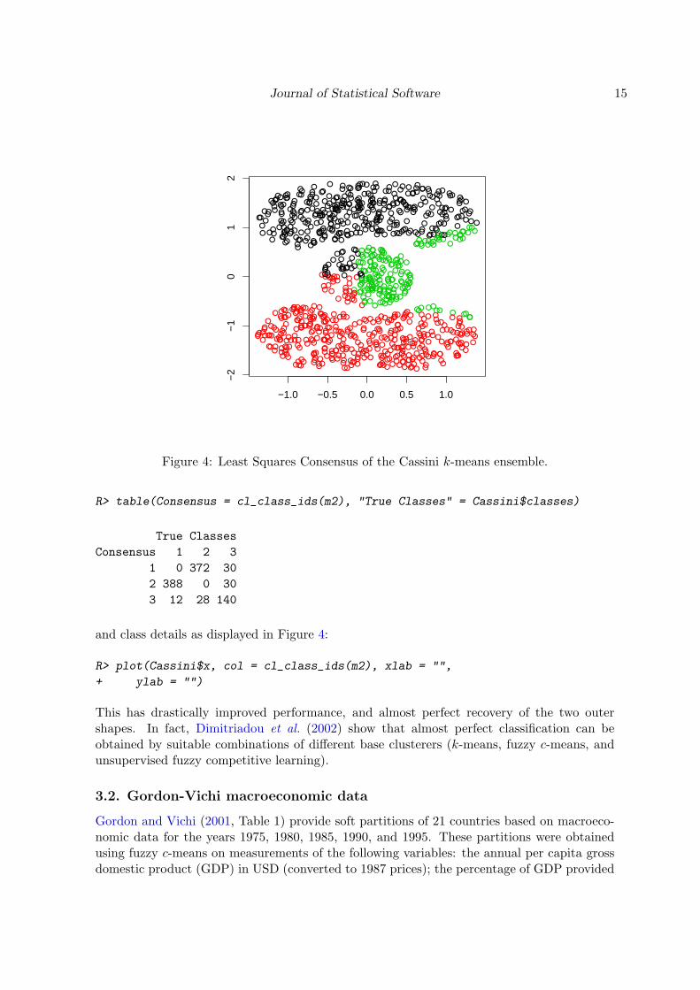
Figure 4: Least Squares Consensus of the Cassini k-means ensemble.

R> table(Consensus = cl_class_ids(m2), "True Classes" = Cassini$classes)

True ClassesConsensus 1 2 3

1 0 372 302 388 0 303 12 28 140

and class details as displayed in Figure 4:

R> plot(Cassini$x, col = cl_class_ids(m2), xlab = "",

+ ylab = "")

This has drastically improved performance, and almost perfect recovery of the two outershapes. In fact, Dimitriadou et al. (2002) show that almost perfect classification can beobtained by suitable combinations of different base clusterers (k-means, fuzzy c-means, andunsupervised fuzzy competitive learning).

3.2. Gordon-Vichi macroeconomic data

Gordon and Vichi (2001, Table 1) provide soft partitions of 21 countries based on macroeco-nomic data for the years 1975, 1980, 1985, 1990, and 1995. These partitions were obtainedusing fuzzy c-means on measurements of the following variables: the annual per capita grossdomestic product (GDP) in USD (converted to 1987 prices); the percentage of GDP provided

16 A CLUE for CLUster Ensembles

by agriculture; the percentage of employees who worked in agriculture; and gross domesticinvestment, expressed as a percentage of the GDP.

Table 4 in Gordon and Vichi (2001) gives 2-class consensus partitions obtained by applyingtheir models 1, 2, and 3 and the approach in Sato and Sato (1994).

The partitions and consensus partitions are available in data sets GVME and GVME_Consensus,respectively. We compare the results of Gordon and Vichi (2001) using Euclidean dissimilar-ities (model 1) to ours as obtained by cl_consensus() with method "GV1".

R> data("GVME")

R> GVME

An ensemble of 5 partitions of 21 objects

R> set.seed(1)

R> m1 <- cl_consensus(GVME, method = "GV1", control = list(k = 2,

+ verbose = TRUE))

Iteration: 1 Old value: 8.37857 New value: 3.005484Iteration: 2 Old value: 3.005484 New value: 3.005484

This results in a soft partition with average Euclidean dissimilarity (the criterion function tobe optimized by the consensus partition) of

R> mean(cl_dissimilarity(GVME, m1)^2)

[1] 3.005484

We compare this to the consensus solution given in Gordon and Vichi (2001):

R> data("GVME_Consensus")

R> m2 <- GVME_Consensus[["MF1"]]

R> mean(cl_dissimilarity(GVME, m2)^2)

[1] 3.538938

R> table(CLUE = cl_class_ids(m1), GV2001 = cl_class_ids(m2))

GV2001CLUE 1 2

1 9 02 5 7

Interestingly, we are able to obtain a “better” solution, which is markedly different from theone reported in the literature, and results in different classifications for the following countries:

R> rownames(m2)[cl_class_ids(m1) != cl_class_ids(m2)]

Journal of Statistical Software 17

[1] "Argentina" "Chile" "Portugal"[4] "South Africa" "Venezuela"

We note however that Gordon and Vichi (2001) solve a different optimization problem, asin the case of partitions with different numbers of classes they only use the matched classeswhen computing dissimilarity, discarding the unmatched ones (see their Example 2). As thisresults in dissimilarity measures which are discontinuous over the space of soft partitions, ourdefinition should be preferred.

3.3. Rosenberg-Kim kinship terms data

Rosenberg and Kim (1975) describe an experiment where perceived similarities of the kinshipterms were obtained from six different “sorting” experiments. In one of these, 85 femaleundergraduates at Rutgers University were asked to sort 15 English terms into classes “onthe basis of some aspect of meaning”. These partitions were printed in Rosenberg (1982,Table 7.1). Comparison with the original data indicates that the partition data have the“nephew” and “niece” columns interchanged, which is corrected in data set Kinship82.

Gordon and Vichi (2001, Table 6) provide consensus partitions for these data based on theirmodels 1–3 (available in data set Kinship82_Consensus). We compare their results using co-membership dissimilarities (model 3) to ours as obtained by cl_consensus() with method"GV3".

R> data("Kinship82")

R> Kinship82

An ensemble of 85 partitions of 15 objects

R> set.seed(1)

R> m1 <- cl_consensus(Kinship82, method = "GV3",

+ control = list(k = 3, verbose = TRUE))

Iteration: 1 Rho: 0.0978703 P: 51.14835Iteration: 2 Rho: 0.978703 P: 0.2692162Iteration: 3 Rho: 9.78703 P: 0.1837687Iteration: 4 Rho: 97.8703 P: 0.03277258Iteration: 5 Rho: 978.703 P: 0.0008170751Iteration: 6 Rho: 9787.03 P: 9.285078e-06Iteration: 7 Rho: 97870.3 P: 9.410234e-08Iteration: 8 Rho: 978703 P: 9.42288e-10Iteration: 9 Rho: 9787030 P: 9.42417e-12Iteration: 10 Rho: 97870297 P: 9.424297e-14Iteration: 11 Rho: 978702969 P: 9.42421e-16Iteration: 12 Rho: 9787029692 P: 9.42384e-18

This results in a soft partition with average co-membership dissimilarity (the criterion functionto be optimized by the consensus partition) of

18 A CLUE for CLUster Ensembles

R> mean(cl_dissimilarity(Kinship82, m1, "comem")^2)

[1] 28.36927

Again, we compare this to the corresponding consensus solution given in Gordon and Vichi(2001):

R> data("Kinship82_Consensus")

R> m2 <- Kinship82_Consensus[["JMF"]]

R> mean(cl_dissimilarity(Kinship82, m2, "comem")^2)

[1] 28.49879

Interestingly, again we obtain a (this time only “slightly”) better solution, with

R> cl_dissimilarity(m1, m2, "comem")

Dissimilarities using euclidean comembership distances:1

1 0.3708913

R> table(CLUE = cl_class_ids(m1), GV2001 = cl_class_ids(m2))

GV2001CLUE 1 2 3

1 0 6 02 4 0 03 0 0 5

indicating that the two solutions are reasonably close, even though

R> cl_fuzziness(cl_ensemble(m1, m2))

Fuzziness using normalized partition coefficient:[1] 0.4360393 0.3894000

shows that our solution is “softer”.

3.4. Miller-Nicely consonant phoneme confusion data

Miller and Nicely (1955) obtained the data on the auditory confusions of 16 English conso-nant phonemes by exposing female subjects to a series of syllables consisting of one of theconsonants followed by the vowel ‘a’ under 17 different experimental conditions. Data setPhonemes provides consonant misclassification probabilities (i.e., similarities) obtained fromaggregating the six so-called flat-noise conditions in which only the speech-to-noise ratio wasvaried into a single matrix of misclassification frequencies.These data are used in de Soete (1986) as an illustration of the SUMT approach for findingleast squares optimal fits to dissimilarities by ultrametrics. We can reproduce this analysisas follows.

Journal of Statistical Software 19

R> data("Phonemes")

R> d <- 1 - as.dist(Phonemes)

(Note that the data set has the consonant misclassification probabilities, i.e., the similaritiesbetween the phonemes.)

R> u <- ls_fit_ultrametric(d, control = list(verbose = TRUE))

Iteration: 1 Rho: 0.04900063 P: 1.241596Iteration: 2 Rho: 0.4900063 P: 0.1532151Iteration: 3 Rho: 4.900063 P: 0.01698076Iteration: 4 Rho: 49.00063 P: 0.0002151106Iteration: 5 Rho: 490.0063 P: 2.288047e-06Iteration: 6 Rho: 4900.063 P: 2.302562e-08Iteration: 7 Rho: 49000.63 P: 2.304022e-10Iteration: 8 Rho: 490006.3 P: 2.304168e-12Iteration: 9 Rho: 4900063 P: 2.304183e-14Iteration: 10 Rho: 49000626 P: 2.304184e-16

This gives an ultrametric u for which Figure 5 plots the corresponding dendrogram,“basically”reproducing Figure 1 in de Soete (1986).

R> plot(u)

We can also compare the least squares fit obtained to that of other hierarchical clusterings ofd, e.g. those obtained by hclust(). The “optimal” u has Euclidean dissimilarity

R> round(sqrt(sum((d - u)^2)), 4)

[1] 0.1988

to d. (Note that we currently cannot use cl_dissimilarity() here, as d does not correspondto a hierarchy.) For the hclust() results, we get

R> hclust_methods <- c("ward", "single", "complete",

+ "average", "mcquitty", "median", "centroid")

R> hens <- cl_ensemble(list = lapply(hclust_methods,

+ function(m) hclust(d, m)))

R> names(hens) <- hclust_methods

R> sapply(hens, function(h) round(sqrt(sum((d - cl_ultrametric(h))^2)),

+ 4))

ward single complete average mcquitty median4.4122 0.4279 0.3134 0.2000 0.2020 4.0168

centroid4.4368

20 A CLUE for CLUster Ensembles

0.0

0.2

0.4

0.6

0.8

1.0

SH

AT

AP

AK

AS

AF

AT

HE

TA

MA

NA

BA

VA

TH

AT

DA

GA

ZA

ZH

AFigure 5: Dendrogram for least squares fit to the Miller-Nicely consonant phoneme confusiondata.

which all exhibit greater Euclidean dissimilarity to d than u. We can also compare the“structure” of the different hierarchies, e.g. by looking at the rate of inversions between them:

R> ahens <- c(L2opt = cl_ensemble(u), hens)

R> round(cl_dissimilarity(ahens, method = "gamma"),

+ 2)

Dissimilarities using rate of inversions:L2opt ward single complete average mcquitty median

ward 0.29single 0.24 0.45complete 0.03 0.29 0.27average 0.03 0.26 0.24 0.03mcquitty 0.03 0.26 0.24 0.03 0.00median 0.79 0.74 0.65 0.79 0.77 0.77centroid 0.77 0.65 0.74 0.79 0.76 0.76 0.88

4. Outlook

Package clue was designed as an extensible environment for computing on cluster ensembles.It currently provides basic data structures for representing partitions and hierarchies, and

Journal of Statistical Software 21

facilities for computing on these, including methods for measuring proximity and obtainingconsensus and “secondary” clusterings.Many extensions to the available functionality are possible and in fact planned (some of theseenhancements were already discussed in more detail in the course of this paper).

• Add data structures for hard/soft partitions based on prototypes.

• Provide mechanisms to generate cluster ensembles based on resampling (assumingprototype-based base partitional clusterers) or reweighting (assuming base clusterersallowing for case weights) the data set.

• Explore recent advances (e.g., parallelized random search) in heuristics for solving themulti-dimensional assignment problem.

• Add support for additive trees (e.g., Barthelemy and Guenoche 1991).

• Add heuristics for finding least squares fits based on iterative projection on convexsets of constraints, see e.g. Hubert, Arabie, and Meulman (2004) and the accompany-ing MATLAB code available at http://cda.psych.uiuc.edu/srpm_mfiles for usingthese methods (instead of SUMT approaches) to fit ultrametrics and additive trees toproximity data.

• Add an“L1 View”. Emphasis in clue, in particular for obtaining consensus clusterings, ison using Euclidean dissimilarities (based on suitable least squares distances); arguably,more “robust” consensus solutions should result from using Manhattan dissimilarities(based on absolute distances). Adding such functionality necessitates developing thecorresponding structure theory for soft Manhattan median partitions. Minimizing av-erage Manhattan dissimilarity between co-memberships and ultrametrics results in con-strained L1 approximation problems for the weighted medians of the co-membershipsand ultrametrics, respectively, and could be approached by employing SUMTs analogousto the ones used for the L2 approximations.

• Provide heuristics for obtaining hard consensus partitions.

• Add facilities for tuning hyper-parameters (most prominently, the number of classesemployed) and “cluster validation” of partitioning algorithms, as recently proposed byRoth, Lange, Braun, and Buhmann (2002) and Dudoit and Fridlyand (2002).

We are hoping to be able to provide many of these extensions in the near future.

Acknowledgments

We are grateful to Walter Bohm for providing efficient C code for solving assignment problems.

References

Barthelemy JP, Guenoche A (1991). Trees and Proximity Representations. Wiley-InterscienceSeries in Discrete Mathematics and Optimization. John Wiley & Sons, Chichester. ISBN0-471-92263-3.

22 A CLUE for CLUster Ensembles

Bertsekas DP, Tseng P (1994). “RELAX-IV: A Faster Version of the RELAX Code forSolving Minimum Cost Flow Problems.” Technical Report P-2276, Massachusetts Instituteof Technology. URL http://www.mit.edu/dimitrib/www/noc.htm.

Bezdek JC (1981). Pattern Recognition with Fuzzy Objective Function Algorithms. Plenum,New York.

Breiman L (1996). “Bagging Predictors.” Machine Learning, 24(2), 123–140.

Buttrey SE (2005). “Calling the lp_solve Linear Program Software from R, S-PLUS andExcel.”Journal of Statistical Software, 14(4). URL http://www.jstatsoft.org/v14/i04/.

Carpaneto G, Toth P (1980). “Algorithm 548: Solution of the Assignment Problem.” ACMTransactions on Mathematical Software, 6(1), 104–111. ISSN 0098-3500.

Carroll JD, Pruzansky S (1980). “Discrete and Hybrid Scaling Models.” In ED Lantermann,H Feger (eds.), “Similarity and Choice,” Huber, Bern, Switzerland.

Day WHE (1986). “Foreword: Comparison and Consensus of Classifications.” Journal ofClassification, 3, 183–185.

de Soete G (1986). “A Least Squares Algorithm for Fitting an Ultrametric Tree to a Dissim-ilarity Matrix.” Pattern Recognition Letters, 2, 133–137.

Dimitriadou E (2005). cclust: Convex Clustering Methods and Clustering Indexes. R packageversion 0.6-12, URL http://CRAN.R-project.org/.

Dimitriadou E, Hornik K, Leisch F, Meyer D, Weingessel A (2005). e1071: Misc Functionsof the Department of Statistics (e1071), TU Wien. R package version 1.5-7, URL http://CRAN.R-project.org/.

Dimitriadou E, Weingessel A, Hornik K (2002). “A Combination Scheme for Fuzzy Clustering.”International Journal of Pattern Recognition and Artificial Intelligence, 16(7), 901–912.

Dudoit S, Fridlyand J (2002). “A Prediction-based Resampling Method for Estimatingthe Number of Clusters in a Dataset.” Genome Biology, 3(7), 1–21. URL http://genomebiology.com/2002/3/7/resarch0036.1.

Dudoit S, Fridlyand J (2003). “Bagging to Improve the Accuracy of a Clustering Procedure.”Bioinformatics, 19(9), 1090–1099.

Fern XZ, Brodley CE (2004). “Solving Cluster Ensemble Problems by Bipartite Graph Parti-tioning.” In“ICML ’04: Twenty-first International Conference on Machine Learning,”ACMPress, New York, USA. ISBN 1-58113-828-5.

Forgy EW (1965). “Cluster Analysis of Multivariate Data: Efficiency vs. Interpretability ofClassifications.” Biometrics, 21, 768–769.

Fowlkes EB, Mallows CL (1983). “A Method for Comparing Two Hierarchical Clusterings.”Journal of the American Statistical Association, 78, 553–569.

Fraley C, Raftery AE (2003). “Enhanced Model-based Clustering, Density Estimation, andDiscriminant Analysis Software: MCLUST.” Journal of Classification, 20(2), 263–286.

Journal of Statistical Software 23

Fraley C, Raftery AE, Wehrens R (2005). mclust: Model-based Cluster Analysis. R packageversion 2.1-11, URL http://www.stat.washington.edu/mclust.

Fred ALN, Jain AK (2002). “Data Clustering Using Evidence Accumulation.” In“Proceedingsof the 16th International Conference on Pattern Recognition (ICPR 2002),” pp. 276–280.URL http://citeseer.ist.psu.edu/fred02data.html.

Friedman J, Hastie T, Tibshirani R (2000). “Additive Logistic Regression: A Statistical Viewof Boosting.” The Annals of Statistics, 28(2), 337–407.

Garey MR, Johnson DS (1979). Computers and Intractability: A Guide to the Theory ofNP-Completeness. W. H. Freeman, San Francisco.

Gentleman R, Whalen E (2005). graph: A Package to Handle Graph Data Structures. Rpackage version 1.5.9, URL http://www.bioconductor.org/.

Gordon AD (1999). Classification. Chapman & Hall/CRC, Boca Raton, Florida, 2nd edition.

Gordon AD, Vichi M (1998). “Partitions of Partitions.” Journal of Classification, 15, 265–285.

Gordon AD, Vichi M (2001). “Fuzzy Partition Models for Fitting a Set of Partitions.” Psy-chometrika, 66(2), 229–248.

Grundel D, Oliveira CA, Pardalos PM, Pasiliao E (2005). “Asymptotic Results for RandomMultidimensional Assignment Problems.” Computational Optimization and Applications,31. In press.

Hansen BB (2005). optmatch: Functions for Optimal Matching. R package version 0.1-3,URL http://www.stat.lsa.umich.edu/~bbh/optmatch.html.

Hartigan JA, Wong MA (1979). “A K-Means Clustering Algorithm.” Applied Statistics, 28,100–108.

Hoeting J, Madigan D, Raftery A, Volinsky C (1999). “Bayesian Model Averaging: A Tuto-rial.” Statistical Science, 14, 382–401.

Hornik K (2005). “Cluster Ensembles.” In C Weihs, W Gaul (eds.), “Classification – TheUbiquitous Challenge,” pp. 65–72. Springer-Verlag, Heidelberg. Proceedings of the 28thAnnual Conference of the Gesellschaft fur Klassifikation e.V., University of Dortmund,March 9–11, 2004.

Hubert L, Arabie P (1995). “Iterative Projection Strategies for the Least Squares Fittingof Tree Structures to Proximity Data.” British Journal of Mathematical and StatisticalPsychology, 48, 281–317.

Hubert L, Arabie P, Meulman J (2004). “The Structural Representation of Proximity Matriceswith MATLAB.” URL http://cda.psych.uiuc.edu/srpm_mfiles.

Katz L, Powell JH (1953). “A Proposed Index of the Conformity of one Sociometric Measure-ment to Another.” Psychometrika, 18, 249–256.

Krieger AM, Green PE (1999). “A Generalized Rand-index Method for Consensus Clusteringof Separate Partitions of the Same Data Base.” Journal of Classification, 16, 63–89.

24 A CLUE for CLUster Ensembles

Krivanek M (1986). “On the Computational Complexity of Clustering.” In E Diday, Y Es-coufier, L Lebart, J Pages, Y Schektman, R Tomassone (eds.), “Data Analysis and Infor-matics 4,” pp. 89–96. Elsevier/North-Holland, Amsterdam.

Krivanek M, Moravek J (1986). “NP-hard Problems in Hierarchical Tree Clustering.” ActaInformatica, 23, 311–323.

Leisch F (1999). “Bagged Clustering.”Working Paper 51, SFB“Adaptive Information Systemsand Modeling in Economics and Management Science”. URL http://www.ci.tuwien.ac.at/~leisch/papers/wp51.ps.

Leisch F (2005). flexclust: Flexible Cluster Algorithms. R package 0.7-0, URL http://CRAN.R-project.org/.

Leisch F, Dimitriadou E (2005). mlbench: Machine Learning Benchmark Problems. R packageversion 1.0-1, URL http://CRAN.R-project.org/.

Lloyd SP (1957). “Least Squares Quantization in PCM.” Technical Note, Bell Laboratories.

Lloyd SP (1982). “Least Squares Quantization in PCM.” IEEE Transactions on InformationTheory, 28, 128–137.

Meila M (2003). “Comparing Clusterings by the Variation of Information.” In B Scholkopf,MK Warmuth (eds.), “Learning Theory and Kernel Machines,” Lecture Notes in ComputerScience, pp. 173–187. Springer-Verlag, Heidelberg.

Miller GA, Nicely PE (1955). “An Analysis of Perceptual Confusions Among some EnglishConsonants.” Journal of the Acoustical Society of America, 27, 338–352.

Mirkin BG (1996). Mathematical Classification and Clustering. Kluwer Academic PublishersGroup.

Oliveira CAS, Pardalos PM (2004). “Randomized Parallel Algorithms for the Multidimen-sional Assignment Problem.” Applied Numerical Mathematics, 49(1), 117–133.

Papadimitriou C, Steiglitz K (1982). Combinatorial Optimization: Algorithms and Complex-ity. Prentice Hall, Englewood Cliffs.

R Development Core Team (2005). R: A Language and Environment for Statistical Computing.R Foundation for Statistical Computing, Vienna, Austria. ISBN 3-900051-07-0, URL http://www.R-project.org.

Rand WM (1971). “Objective Criteria for the Evaluation of Clustering Methods.” Journal ofthe American Statistical Association, 66(336), 846–850.

Rosenberg S (1982). “The Method of Sorting in Multivariate Research with Applications Se-lected from Cognitive Psychology and Person Perception.” In N Hirschberg, LG Humphreys(eds.), “Multivariate Applications in the Social Sciences,” pp. 117–142. Erlbaum, Hillsdale,New Jersey.

Rosenberg S, Kim MP (1975). “The Method of Sorting as a Data-gathering Procedure inMultivariate Research.” Multivariate Behavioral Research, 10, 489–502.

Journal of Statistical Software 25

Roth V, Lange T, Braun M, Buhmann JM (2002). “A Resampling Approach to Cluster Vali-dation.” In W Hardle, B Ronz (eds.), “COMPSTAT 2002 – Proceedings in ComputationalStatistics,” pp. 123–128. Physika Verlag, Heidelberg, Germany. ISBN 3-7908-1517-9.

Rousseeuw P, Struyf A, Hubert M, Maechler M (2005). cluster: Functions for Clustering (byRousseeuw et al.). R package version 1.9.8, URL http://CRAN.R-project.org/.

Sato M, Sato Y (1994). “On a Multicriteria Fuzzy Clustering Method for 3-way Data.”International Journal of Uncertainty, Fuzziness and Knowledge-based Systems, 2, 127–142.

Sokal RR, Rohlf FJ (1962). “The Comparisons of Dendrograms by Objective Methods.”Taxon, 11, 33–40.

Strehl A, Ghosh J (2003a). “Cluster Ensembles – A Knowledge Reuse Framework for Com-bining Multiple Partitions.” Journal of Machine Learning Research, 3, 583–617. ISSN1533-7928.

Strehl A, Ghosh J (2003b). “Relationship-based Clustering and Visualization for High-Dimensional Data Mining.” INFORMS Journal on Computing, 15, 208–230. ISSN 1526-5528.

Struyf A, Hubert M, Rousseeuw P (1996). “Clustering in an Object-Oriented Environment.”Journal of Statistical Software, 1(4). URL http://www.jstatsoft.org/v01/i04/.

Wallace DL (1983). “Comments on“A Method for Comparing Two Hierarchical Clusterings”.”Journal of the American Statistical Association, 78, 569–576.

Affiliation:

Kurt HornikDepartment fur Statistik und MathematikWirtschaftsuniversitat Wien1090 Wien, AustriaTelephone: +43/1/31336-4756Fax: +43/1/31336-774E-mail: Kurt.Hornik@wu-wien.ac.atURL: http://www.wu-wien.ac.at/cstat/hornik

Journal of Statistical Software Submitted: 2005-05-13September 2005, Volume 14, Issue 12. Accepted: 2005-09-20http://www.jstatsoft.org/