A class of perturbed cell-transmission models to account...

A class of perturbed cell-transmission models to

account for traffic variability

S. Blandin∗ D. Work† P. Goatin‡ B. Piccoli§ A. Bayen¶

Submitted For Publication

89th Annual Meeting of the Transportation Research Board

August 1, 2009

Word Count:

Number of words: 6122Number of figures: 4 (250 words each)Number of tables: 0 (250 words each)Total: 7122

∗Corresponding Author, PhD student, Systems Engineering, Department of Civil and Environ-mental Engineering, UC Berkeley, 621 Sutardja Dai Hall, Berkeley, CA 94720-1720, USA. E-mail:[email protected]

†PhD student, Systems Engineering, Department of Civil and Environmental Engineering, UCBerkeley, 621 Sutardja Dai Hall, Berkeley, CA 94720-1720, USA. E-mail: [email protected]

‡Assistant Professor, Institut de Mathematiques de Toulon et du Var, I.S.I.T.V., Universite duSud Toulon-Var, La Valette du Var, France. E-mail: [email protected]

§Research Director, Istituto per le Aplicazioni del Calcolo ‘M.Picone’, Roma, Italy. E-mail:[email protected]

¶Assistant Professor, Systems Engineering, Department of Civil and Environmental Engineering,UC Berkeley, 642 Sutardja Dai Hall, Berkeley, CA 94720-1720, USA. E-mail: [email protected]

1

A class of perturbed cell transmission models to account for traffic variability S. Blandin, D. Work, P. Goatin, B. Piccoli and A. Bayen 89th Annual Meeting of the Transportation Research Board, Washington D.C., January 10-14, 2010

Abstract

We introduce a general class of traffic models derived as perturbations ofcell-transmission type models. These models use different dynamics in free-flowand in congestion phases. They can be viewed as extensions to cell transmissiontype models by considering the velocity to be a function not only of the densitybut also of a second state variable describing perturbations. We present themodels in their discretized form under a new formulation similar to the classicalsupply demand formulation used by the seminal Cell-Transmission Model. Wethen show their equivalence to hydrodynamic models. We detail the proper-ties of these so-called perturbed cell-transmission models and illustrate theirmodeling capabilities on a simple benchmark case. It is shown that they en-compass several well-known phenomena not captured by classical models, suchas forward moving disturbances occurring inside congestion phases. An imple-mentation method is outlined which enables to extend the implementation ofa cell transmission model to a perturbed cell transmission model.

2


1 Introduction1

Classical macroscopic models of traffic. The modeling of highway traffic at a2

macroscopic level is a well established field in the transportation engineering commu-3

nity, which goes back to the seminal work of Lighthill, Whitham [17] and Richards [23].4

Their work introduced to the traffic community the kinematic wave theory which en-5

ables one to reconstruct fundamental macroscopic features of traffic flow on highways6

such as queues propagation. The so-called LWR model, based on conservation of7

vehicles, encompasses most of the non linear phenomena observed on highways in a8

computationally tractable framework.9

In order to close the model, one needs to assume a relation between the velocity10

and density of vehicles. Greenshields [13] empirically measured a relation between the11

density and the flow of vehicles, now known as the fundamental diagram, which led12

to the formulation of the LWR problem as a single unknown state variable problem,13

which could be solved by discretization techniques.14

A way to approach the resolution of the discretization of the mass conservation15

equation in a tractable manner was later proposed by Lebacque [15]. It was shown16

that a discrete solution of the LWR equation could be constructed by considering17

the local supply demand framework. In the case of concave fluxes, this solution is18

equivalent to the one obtained using a classical numerical method in conservation19

laws, the Godunov scheme [12].20

The triangular model. Newell [18, 19, 20] introduced the triangular funda-21

mental diagram, which is to this date one of the most standard models for queuing22

phenomena observed at bottlenecks, and for highway traffic modeling in general. Da-23

ganzo [7, 8] derived a discrete equivalent of the LWR equation in the case of the24

triangular fundamental diagram. This model known as the Cell-Transmission Model25

provided the transportation community with a meaningful modeling tool for highway26

traffic. One of the main assumptions of all the classical models is that the speed of27

vehicles is a single-valued function of the density.28

Second order and perturbed models. Following hydrodynamic theory, at-29

tempts at modeling highway traffic with a second conservation equation and a second30

state variable to augment the mass conservation equation led to the development of31

so-called second order models, such as the Payne [22] and Whitham [25] model. Un-32

fortunately, this model exhibited flaws pointed out by Daganzo [9], Del Castillo [10]33

and Papageorgiou [21], including the possibility for vehicles to drive backwards along34

the highway. These flaws were corrected in a new generation of second order models35

proposed for instance by Aw and Rascle [3], Lebacque [16] and Zhang [28, 29]. By36

considering a second state variable, these models offer additional capabilities with37

respect to classical models and for example enable the possibility to include velocity38

measurements such as the ones obtained from GPS cell phones [26].39

The phase transition model Colombo [6] developed a phase transition traffic40

model with different dynamics for congestion and free-flow, to model fundamental di-41

agrams observed in practice [1]. Like the work of Newell, this approach was motivated42

by the fundamentally different features of traffic in free-flow and in congestion [24].43

In particular, this model includes a set-valued congested part of the fundamental di-44

3


agram and a single-valued free-flow part of the fundamental diagram. The set-valued45

congestion phase enables one to account for much more measurements in the con-46

gestion phase than the classical fundamental diagram does. Indeed, in the classical47

setting, a measurement falling outside of the fundamental diagram has to be discarded48

or approximated. Thus for any tasks involving real data, information is lost at the49

data processing step. In the setting proposed by the phase transition model and the50

subsequent perturbed cell transmission model, a whole cloud of measurements can be51

considered valid.52

In part due to the complexity of practical implementation, Colombo’s model was53

extended in [5], leading to a new class of models taking in account the perturbation54

around the classical fundamental diagram known to exist in practice. Similar to the55

work of Zhang [28], an assumption is made that a classical fundamental diagram can56

be viewed as an equilibrium (or average) of the highway traffic state in the perturbed57

model. In this article, we describe the physical approach developed in [5] and present58

simple and meaningful local rules to implement a class of discrete perturbed models.59

We also provide a set of simple steps which can be followed to extend the well-known60

implementation of the cell-transmission model to an implementation of a perturbed61

cell transmission model.62

Outline. The outline of this work is as follows. In Section 2, we recall the classical63

framework for discrete macroscopic models, and introduce the discrete formulation of64

a class of phase transition models relying on physical consideration about traffic flow65

properties. In particular we show that these models reduce to a set-valued version66

of the cell-transmission model in the case of a triangular flux. Section 3 provides67

some examples of the modeling abilities of the class of perturbed models derived, and68

illustrates the better performances of the class of perturbed models. Section 4 gives a69

guidebook for perturbed model deployment. Conclusions and future research tracks70

are outlined in Section 5.71

2 Discrete formulation of macroscopic traffic flow72

models73

We consider the representation of a stretch of highway by N space cells Cs, 0 ≤ s ≤ N74

of size ∆x and assume that representing time evolution by a discrete sequence of times75

with a ∆t step size yields a correct approximation for traffic flow modeling.76

We make the usual assumption that there is no ramp on the link of interest, and77

assume by considering a one-dimensional representation of the traffic conditions that78

even on a multi-lanes highway, traffic phenomena can be accurately modeled as one79

lane highway. The results presented here can easily be generalized to networks, for80

example using the framework developed by Piccoli [11].81

The following section presents the fundamental macroscopic traffic modeling equa-82

tion, i.e. the mass conservation.83

4


2.1 Classical models84

2.1.1 Mass conservation equation85

We call kts the density of vehicles in the space cell Cs at time t, and Qt

s-up (respectivelyQt

s-down) the flux upstream (respectively downstream) of cell s between time t andtime t+1. The absence of ramp in cell s allows us to write the following conservationequation for the density of vehicles in cell s:

kt+1s ∆x − kt

s ∆x = Qts-up ∆t − Qt

s-down ∆t (1)

which states that between two consecutive times the variation of the number of vehi-86

cles cell Cs is exactly equal to the difference between the number of vehicles having87

entered the cell from upstream and the number of vehicles having exited the cell from88

downstream.89

Equation (1) which is the mass conservation from fluid dynamics (in a discrete90

setting) is widely used among the transportation engineering community and consid-91

ered as one of the most meaningful ways to model traffic flow on highways. Defining92

the fluxes Qs-down, Qs-up between two cells is a more complex problem, which can be93

approached by considering a supply demand formulation.94

2.1.2 The supply demand approach95

The supply demand approach [15] states that the flow of cars that can travel from96

an upstream cell to the next downstream cell depends on both the upstream density97

and the downstream density. If we define the demand function ∆(·) as a continu-98

ous increasing function of the density and the supply function Σ(·) as a continuous99

decreasing function of the density, then the flux between two cells is given by the100

minimum of the upstream demand and the downstream supply. The supply and de-101

mand function are bounded above on each cell by the flow capacity of the cell. Using102

the notations introduced above, the supply demand formulation reads:103

Qts-up = min(∆(kt

s−1), Σ(kts)) (2)

Qts-down = min(∆(kt

s), Σ(kts+1)).

The demand and supply functions are related to the fundamental diagram as follows.104

In free-flow the supply Σ(·) is simply limited by the capacity of the cell whereas105

in congestion, the supply is limited by current traffic conditions. In free-flow, the106

demand ∆(·) is limited by current traffic conditions whereas in congestion the demand107

is constrained by the capacity of the cell. Given a fundamental diagram Q(·), with a108

unique maximum at the critical density kc, the supply Σ(·) and demand ∆(·) functions109

can thus be defined as:110

∆(k) =

{

Q(k) if k ≤ kc

Q(kc) otherwiseand Σ(k) =

{

Q(kc) if k ≤ kc

Q(k) otherwise

5


Q

k

Figure 1: Supply demand. The supply curve (bold line) is an increasing functionof density and the demand curve (dashed line) is a decreasing function of density.

When the fundamental diagram is triangular, the demand and supply functions are111

piecewise affine as illustrated on Figure 1, and the supply demand approach is exactly112

the cell-transmission model [7].113

The supply demand approach enables one to define two types of traffic conditions;114

free-flow and congestion, which have fundamentally different features.115

2.2 Two traffic phases116

The behavior of traffic depends on the relative values of supply and demand. When117

the supply is higher than the demand, traffic flow is said to be in free-flow, the flux is118

defined by the number of cars that can be sent from upstream (upstream demand).119

On the opposite, when the demand is higher than the supply, the traffic is said to120

be in congestion because the flux is defined by the number of cars that the road can121

accept downstream (downstream supply).122

These two dynamics exhibit at least one capital difference:123

• In free-flow the flux is defined from upstream and information is moving forward,124

whereas in congestion the flux is defined from downstream and information is125

moving backwards.126

One may note that the seminal Cell-Transmission Model considers this property as a127

required model feature, and thus can be viewed as a phase transition model. Figure 2128

illustrates two typical sets of experimental measurements. Two distinct phases appear129

characterized by:130

• In free-flow, the speed is constant and the flux is uniquely determined by the131

density of cars (straight line through the origin for low densities in Figure 2).132

The knowledge of density or count seems to provide enough information to133

represent the traffic state.134

6


0 100 200 3000

1000

2000

3000

3500

Q(v

eh/hou

r)

k(veh/mile)0 100 200 250

0

1000

2000

3000

4000

Q(v

eh/hou

r)

k(veh/mile)

Figure 2: Experimental flow-density relations over a one week-period at two locationson a highway in Roma. Flow was directly measured and density was computed fromthe measured flow and the measured speed. In free-flow the speed is constant. Theshape of the congestion phase changes for different locations.

• In congestion, a given density does not correspond to a unique speed, i.e. the135

fundamental diagram is set-valued. A second variable must be introduced to136

model the traffic state.137

The first observation is taken in account by the triangular model whereas the second138

observation motivates the use of a phase transition model [5, 6] using different dynam-139

ics for free-flow and congestion, and justify the introduction of a perturbed model in140

congestion to define the dynamics of two variables necessary to model the congested141

traffic state [24, 27]. We introduce in the following section a class of perturbed cell142

transmission type models directly derived from classical models.143

2.3 Perturbation of cell-transmission type models144

2.3.1 A perturbed fundamental diagram145

We propose to describe traffic state on a link of highway by using a perturbed phase146

transition model. Assuming that the highway link is composed of the cells Cs for147

s = 1, · · · , N , we define the speed of traffic in each cell as follows:148

vs =

{

Vff if Cs is in free-flow

V (ks) (1 + qs) if Cs is in congestion(3)

where Vff is the free-flow speed and V (·) is the velocity function of a classical model.149

Application to the cell transmission model The velocity function for the150

classical cell transmission model reads V (ks) = w(1−kj/ks) where w is the backwards151

speed propagation and kj is the jam density. Thus the perturbed speed reads:152

7


Q

kkj

Q

kkj

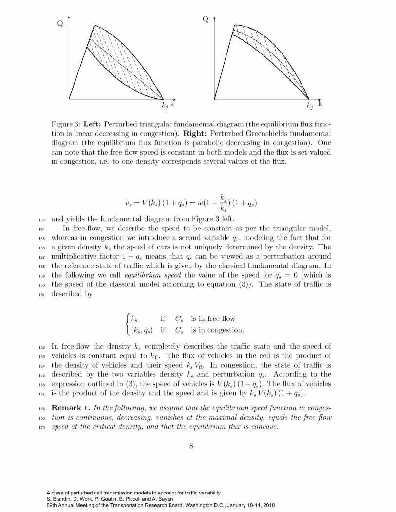
Figure 3: Left: Perturbed triangular fundamental diagram (the equilibrium flux func-tion is linear decreasing in congestion). Right: Perturbed Greenshields fundamentaldiagram (the equilibrium flux function is parabolic decreasing in congestion). Onecan note that the free-flow speed is constant in both models and the flux is set-valuedin congestion, i.e. to one density corresponds several values of the flux.

vs = V (ks) (1 + qs) = w(1 −kj

ks) (1 + qs)

and yields the fundamental diagram from Figure 3 left.153

In free-flow, we describe the speed to be constant as per the triangular model,154

whereas in congestion we introduce a second variable qs, modeling the fact that for155

a given density ks the speed of cars is not uniquely determined by the density. The156

multiplicative factor 1 + qs means that qs can be viewed as a perturbation around157

the reference state of traffic which is given by the classical fundamental diagram. In158

the following we call equilibrium speed the value of the speed for qs = 0 (which is159

the speed of the classical model according to equation (3)). The state of traffic is160

described by:161

{

ks if Cs is in free-flow

(ks, qs) if Cs is in congestion.

In free-flow the density ks completely describes the traffic state and the speed of162

vehicles is constant equal to Vff. The flux of vehicles in the cell is the product of163

the density of vehicles and their speed ks Vff. In congestion, the state of traffic is164

described by the two variables density ks and perturbation qs. According to the165

expression outlined in (3), the speed of vehicles is V (ks) (1 + qs). The flux of vehicles166

is the product of the density and the speed and is given by ks V (ks) (1 + qs).167

Remark 1. In the following, we assume that the equilibrium speed function in conges-168

tion is continuous, decreasing, vanishes at the maximal density, equals the free-flow169

speed at the critical density, and that the equilibrium flux is concave.170

8


Remark 2. For the sake of mathematical and physical consistency, the size of the171

perturbation qs cannot be chosen arbitrarily and must satisfy the following constraints:172

• The perturbed speed must be positive, i.e. qs ≥ −1.173

• The curves on which qs/ks is constant (see section 2.3.3 for a physical inter-174

pretation of these curves) have a concavity with constant sign. This yields a175

bound on the perturbation which can be analytically computed by writing that176

the second derivative of the flux ks V (ks) (1 + qs) with respect to the density ks177

has a constant sign for a given value of qs/ks.178

2.3.2 Conservation equations for traffic states179

Having defined the state of traffic in congestion and in free-flow, we define the dy-180

namics of these quantities as follows. The density ks is assumed to satisfy the mass181

conservation given by equation (1). We assume that the macroscopic perturbation182

qs ∆x is also conserved, and thus that qs satisfies the perturbation conservation equa-183

tion:184

qt+1s ∆x − qt

s ∆x = Rts-up ∆t − Rt

s-down ∆t (4)

where Rts-up (respectively Rt

s-down) is the flow of macroscopic perturbation entering185

the cell Cs from upstream (respectively exiting from downstream). The dynamics186

satisfied by the traffic states is:187

kt+1s ∆x − kt


s-down ∆t in free-flow{

kt+1s ∆x − kt


s-down ∆t

qt+1s ∆x − qt

s ∆x = Rts-up ∆t − Rt

s-down ∆tin congestion

(5)

One must be careful that at any location, the flux of mass Qs-up and the flux of188

perturbation Rs-up are coupled by the relation (3) defining the speed and thus can not189

be defined independently by two uncoupled supply demand relations similar to (2).190

A coherent approach to the definition of the cell boundary fluxes is to consider the191

microscopic meaning of the state variable qs.192

2.3.3 From a macroscopic perturbed model to a behavioral driver model193

Equation (4) expresses the conservation of the macroscopic perturbation qs ∆x. The194

usual classical fundamental diagram corresponds to the equilibrium velocity function195

(i.e. at qs = 0), and for a given density this velocity function can take values above196

or below the equilibrium velocity function depending on the sign of qs.197

This variation of the velocity function around its equilibrium value leads us to198

consider the state variable qs as characterizing the propension of an element of traffic199

to move forward, in a very similar way to the driver’s ride impulse from [2]. Indeed,200

in a cell Cs with a density of vehicles ks, high values of qs model aggressive drivers201

who are eager to move forward and adopt high speed. Low values of qs model passive202

drivers who adopt low values of speed.203

9


The speed vs of drivers and their average aggressiveness defined by the quantity204

qs/ks will play a decisive role in the definition of the boundary fluxes.205

Remark 3. One may note that it is not possible to measure the aggressiveness level of206

drivers. According to the definition of our class of model, this quantity is completely207

determined by the knowledge of the speed and density. Thus measures of counts or208

speeds can be combined with measures of density in order to compute values of the209

aggressiveness level.210

2.3.4 Traffic rules defining flow between cells211

The supply demand formulation does not yield a simple formalism for perturbed212

models. We choose to define the fluxes from equation (5) by other equivalent physical213

considerations. We propose two different sets of rules depending on whether the traffic214

state in the upstream cell is in free-flow or in congestion.215

Congested upstream cell216

We consider two neighboring cells Cs−1 and Cs with traffic states (kts−1, qt

s−1) and217

(kts, q

ts) such that the upstream cell is in a congested state. We define the following218

two rules who will define the flux between these two cells between times t and t + 1:219

• To enter the downstream cell, the vehicles from the upstream cell must modify220

their speed from vts−1 to the speed of the vehicles from the downstream cell vt

s.221

• The vehicle from the upstream cell modify their speed according to their average222

driving aggressiveness qs/ks.223

These two rules imply that the vehicles which will exit the upstream cell Cs−1 to enter224

the downstream cell Cs will have speed vs and will have an average aggressiveness225

qs/ks. Thus the flux between cell Cs−1 and cell Cs correspond to a new traffic state226

(kt+1/2

s−1/2, q

t+1/2

s−1/2) which can be defined by the system of equations:227

qt+1/2

s−1/2

kt+1/2

s−1/2

=qs−1

ks−1

and vt+1/2

s−1/2= vs (6)

where the second equation can be rewritten as an equation in (kt+1/2

s−1/2, q

t+1/2

s−1/2) us-228

ing the expression from (3). This yields a system of two independent equations in229

(kt+1/2

s−1/2, q

t+1/2

s−1/2). The corresponding speed v

t+1/2

s−1/2can be computed from the expression230

of kt+1/2

s−1/2and q

t+1/2

s−1/2using equation (3). The mass flux and perturbation flux can be231

then defined as:232

Qts-up = k

t+1/2

s−1/2v

t+1/2

s−1/2and Rt

s-up = qt+1/2

s−1/2v

t+1/2

s−1/2

10


Free-flowing upstream cell233

We consider two neighboring cells Cs−1 and Cs with traffic states kts−1 (free-flow) and234

(kts, q

ts) (congestion). The boundary flux of vehicles between the upstream cell Cs−1235

and the downstream cell Cs falls into one of these two cases:236

• If the upstream flow is lower than the downstream flow then traffic conditions237

are imposed from upstream and the boundary flow is the upstream flow. This238

leads to the boundary flow:239

Qts-up = kt

s−1 V and Rts-up = q

t+1/2

s−1/2V

where qt+1/2

s−1/2is the perturbation defined by V (kt

s−1) (1 + qt+1/2

s−1/2) = V .240

• If the upstream flow is higher than the downstream flow then traffic conditions241

are imposed from downstream and we obtain similar conditions to the case of242

two congested cells. Incoming vehicles will adapt their speed to the downstream243

speed and adopt the lowest corresponding average level of aggressiveness allow-244

able by the fundamental diagram. These two conditions yield the equations:245

qt+1/2

s−1/2

kt+1/2

s−1/2

=qmin

kj

and vt+1/2

s−1/2= vs (7)

where qmin, kj are the minimal density of perturbation and jam density (maximal246

density). If we note (kt+1/2

s−1/2, q

t+1/2

s−1/2) the solution of (7), the boundary fluxes are247

given by:248

Qts-up = k

t+1/2

s−1/2v

t+1/2

s−1/2and Rt

s-up = qt+1/2

s−1/2v

t+1/2

s−1/2

3 Benchmark cases249

3.1 Encounter of two flows with different properties250

3.1.1 Perturbed model features251

We consider the situation of two cells with congested flows. In the upstream cell the252

traffic state is (kA, qA) with high density and low speed and in the downstream cell253

the state is (kB, qB) with low density and high speed. These two traffic states are254

represented by the points A and B on Figure 4 (right).255

According to the rules described in section 2.3.4, the cars from the upstream cell256

will increase their speed while keeping the same average aggressiveness level qA/kA.257

Physically this means that the drivers from the traffic state A which is slower and258

denser increase their speed when they reach the front end of the flow A, but do not259

change their behavior.260

11


k

QB1

A

B

A1

k

Q

A

B

C

Figure 4: Left: Classical model. A and B fall outside of the classical fundamentaldiagram and are viewed as A1 and B1; the resulting steady state is B1. Right: Per-

turbed model. A and B fall in the perturbed fundamental diagram; the resultingsteady state is C.

Thus the flow of cars moving from the upstream cell to the downstream cell will261

be in state C, defined by the intersection of two curves. The first curve is the straight262

line defined by the speed being the speed of B, namely vC = V (kB, qB) according to263

expression (3). The second curve is defined by the average aggressiveness of drivers264

being the average aggressiveness of drivers from state A, namely qC/kC = qA/kA.265

One can note that this set of two equations is the one introduced at (6).266

3.1.2 Comparison of perturbed and classical model267

We compare the evolution predicted by a classical model and by its associate per-268

turbed model, for the two flows described in previous section. The evolution given269

by the perturbed model was described in previous section.270

The classical model can not take in account the states A and B as such because271

they fall outside of the classical fundamental diagram. Joint measurements of speed272

and density returning traffic states A and B would have to be approximated. They273

could be understood as states A1 and B1 if the density measurement were more274

reliable.275

The interaction of states A1 and B1 is described by the cell-transmission model as276

producing the steady state B1. One can note that this state is significatively different277

from the steady state C predicted by the perturbed model.278

3.2 Homogeneous in speed states279

Traffic flows composed of various densities in which all the vehicles drive at the same280

speed are commonly observed but cannot be accounted for by classical models which281

assume that for one given density, only one speed can occur.282

Perturbed models allow traffic states with different densities to have the same283

12


speed, and can model the homogeneous in speed states observed by Kerner [14]. For284

instance, if we consider the encounter of two traffic flows with the same speed and285

different densities such as the state B and C from Figure 4, the model predicts that286

the difference in flows and densities between the two traffic states is such that the287

discontinuity propagates downstream at exactly the same speed. It is the similar288

situation that is observed in free-flow for the triangular model. Indeed one could289

imagine that the straight line of constant speed defined by v = vC is the free-flow290

part of a classical triangular fundamental diagram, in which case the same type of291

propagation of the two states B and C would be predicted by the cell-transmission292

model.293

4 Implementing a perturbed cell-transmission294

model295

In this section we propose to give a brief outline of the way to implement a perturbed296

cell-transmission model.297

1 Define a classical fundamental diagram which fits the dataset best. Depending on298

the implementation constraints, this can be done in a variety of methods, from a299

visual agreement to an optimization routine [4]. In particular, identify the free-flow300

speed Vff, the jam density kj and the critical density kc. This corresponds to the301

classical implementation method for the CTM.302

2 Compute bounds on the perturbation according to the limitations expressed in303

remark 2. This requires to compute the maximum and minimum of the second304

derivative of the flux function along a curve of constant aggressiveness level.305

3 Given a traffic condition, i.e. a point (ρ, q), check that all the discrete congested306

states fall into the fundamental diagram, otherwise use an approximation method307

to map it back to the fundamental diagram, similarly to the case of the classical308

fundamental diagram.309

4 Evolve the model in time using the rules proposed in section 2.3.4.310

This shows that implementing a perturbed cell-transmission model is almost as311

simple as implementing the classical cell-transmission model. We illustrated in sec-312

tion 3 the added value of these models.313

5 Conclusion314

In this article we propose a class of perturbed models which match empirical features315

of highway traffic more closely than classical models by incorporating a set-valued316

fundamental diagram in congestion. We show that by considering a second state317

variable in congestion, this class of models has greater modeling capabilities.318

13


We follow the principles of the cell-transmission model which assumes that the two319

phases of traffic, free-flow and congestion, have fundamentally different behaviors. We320

consider that the speed of traffic is constant in free-flow whereas in congestion it has a321

perturbed value around the equilibrium speed. The class of models introduced is cus-322

tomizable in the sense that traffic engineers can select the most appropriate classical323

fundamental diagram and perturb it according to experimental measurements.324

We make the assumption that the state variable introduced satisfies a conserva-325

tion equation, which is motivated by its physical interpretation. At the macroscopic326

level, it can be considered as a perturbation of the traffic state around the classical327

fundamental diagram. At a microscopic level, this variable models the behavior of328

drivers, who make different speed choices for the same observed density. We provide329

simple meaningful rules to march the model forward in time.330

Finally, we provide a simple way to implement this perturbed class of traffic331

models in the framework currently used by traffic engineers. We show that these332

models which result from an extension of usual cell-transmission type models can be333

derived in a straightforward manner.334

References335

[1] Freeway Performance Measurement System. http://pems.eecs.berkeley.edu/.336

[2] R. Ansorge. What does the entropy condition mean in traffic flow theory?337

Transportation Research Part B, 24(B):133–143, 1990.338

[3] A. Aw and M. Rascle. Resurrection of “second order” models of traffic flow.339

SIAM Journal on Applied Mathematics, 60(3):916–938, 2000.340

[4] S. Blandin, G. Bretti, A. Cutolo, and B. Piccoli. Numerical simulations of341

traffic data via fluid dynamic approach. Applied mathematics and computation,342

2009 (to appear).343

[5] S. Blandin, D. Work, P. Goatin, B. Piccoli, and A. Bayen. A general344

phase transition model for vehicular traffic. Submitted to SIAM Journal on345

Applied Mathematics, 2009.346

[6] R. Colombo. Hyperbolic phase transitions in traffic flow. SIAM Journal on347

Applied Mathematics, 63(2):708–721, 2003.348

[7] C. Daganzo. The cell transmission model: a dynamic representation of highway349

traffic consistent with the hydrodynamic theory. Transportation Research Part350

B, 28(4):269–287, 1994.351

[8] C. Daganzo. The cell transmission model, part II: Network traffic. Transporta-352

tion Research Part B, 29(2):79–93, 1995.353

[9] C. Daganzo. Requiem for second-order fluid approximations of traffic flow.354

Transportation Research Part B, 29(4):277–286, 1995.355

14


[10] J. Del Castillo, P. Pintado, and F. Benitez. The reaction time of drivers356

and the stability of traffic flow. Transportation research Part B, 28(1):35–60,357

1994.358

[11] M. Garavello and B. Piccoli. Traffic flow on networks. American Institute359

of Mathematical Sciences, Springfield, USA, 2006.360

[12] S. Godunov. A difference method for numerical calculation of discontinuous so-361

lutions of the equations of hydrodynamics. Matematicheskii Sbornik, 89(3):271–362

306, 1959.363

[13] B. Greenshields. A study of traffic capacity. Proceedings of the Highway364

Research Board, 14(1):448–477, 1935.365

[14] B. Kerner. Phase transitions in traffic flow. Traffic and granular flow, pages366

253–283, 2000.367

[15] J.P. Lebacque. The godunov scheme and what it means for first order macro-368

scopic traffic flow models. Proceedings of the 13th ISTTT, Ed. J.B. Lesort,, pages369

647–677, Lyon, 1996.370

[16] J.P. Lebacque, X. Louis, S. Mammar, B. Schnetzler, and H. Haj-Salem.371

Modelling of motorway traffic to second order. Comptes rendus-Mathematique,372

346(21-22):1203–1206, 2008.373

[17] M. Lighthill and G. Whitham. On kinematic waves II a theory of traf-374

fic flow on long crowded roads. Proceedings of the Royal Society of London,375

229(1178):317–345, 1956.376

[18] G. Newell. A simplified theory of kinematic waves in highway traffic, I: General377

theory. Transportation research Part B, 27(4):281–287, 1993.378

[19] G. Newell. A simplified theory of kinematic waves in highway traffic, II: Queue-379

ing at freeway bottlenecks. Transportation research Part B, 27(4):289–303, 1993.380

[20] G. Newell. A simplified theory of kinematic waves in highway traffic, III:381

Multi-destination flows. Transportation research Part B, 27(4):305–313, 1993.382

[21] M. Papageorgiou. Some remarks on macroscopic traffic flow modelling. Trans-383

portation Research Part A, 32(5):323–329, 1998.384

[22] H. Payne. Models of freeway traffic and control. Mathematical models of public385

systems, 1(1):51–61, 1971.386

[23] P. Richards. Shock waves on the highway. Operations Research, 4(1):42–51,387

1956.388

[24] P. Varaiya. Reducing highway congestion: an empirical approach. European389

journal of control, 11(4-5):301–309, 2005.390

15


[25] G. Whitham. Linear and Nonlinear Waves. Pure & Applied Mathematics391

Series, New York: Wiley-Interscience, 1974.392

[26] D. Work and A. Bayen. Impacts of the mobile internet on transportation393

cyberphysical systems: traffic monitoring using smartphones. In National Work-394

shop for Research on High-Confidence Transportation Cyber-Physical Systems:395

Automotive, Aviation and Rail, Washington, D.C., 2008.396

[27] J. Yi, H. Lin, L. Alvarez, and R. Horowitz. Stability of macroscopic traffic397

flow modeling through wavefront expansion. Transportation Research Part B,398

37(7):661–679, 2003.399

[28] H. Zhang. A theory of nonequilibrium traffic flow. Transportation Research400

Part B, 32(7):485–498, 1998.401

[29] H. Zhang. A non-equilibrium traffic model devoid of gas-like behavior. Trans-402

portation Research Part B, 36(3):275–290, 2002.403

16


A class of perturbed cell-transmission models to account...

Documents

Transcript of A class of perturbed cell-transmission models to account...