A class of low order DIRK methods for a class of DAEs

Applied Numerical Mathematics 31 (1999) 1–16

A class of low order DIRK methods for a class of DAEs

Frank Cameron1

Tampere University of Technology, P.O. Box 692, 33101 Tampere, Finland

Abstract

We study the numerical solution of a DAE described by an implicit differential equation where the state derivativeis multiplied by a singular matrix that depends on the state. We consider a class ofs-stage DIRK methods havings − 1 implicit stages, an explicit first stage and the stiff accuracy property. The DIRKs we consider have globalorder of at most 3. We determine how many stages are required to meet different order and stability specifications,both for solitary (fixed step size) DIRKs as well as embedded pairs of DIRKs. We present some solitary DIRKsand some embedded DIRK pairs that have appeared in the literature and that are suitable for solving the DAE inquestion. In addition, we derive some new solitary DIRKs and DIRK pairs. Our tests with embedded pairs showthat some pairs may suffer from performance deterioration when the dynamics in the DAE are of different ordersof magnitude. 1999 Elsevier Science B.V. and IMACS. All rights reserved.

Keywords:Differential–algebraic systems; Runge–Kutta methods

1. Introduction

The initial value problem

S(y)y′ = f (y, t), y(t0)= y0 (1)

with singularS(y) arises in the modeling of circuits, chemical kinetics and transient electro-magneticphenomena [4,13]. We assume here thatS(y) has constant rank, and that (1) has differential index 1 [8,Chapter 1]. In this paper we study a class of easily-implementable low-order implicit Runge–Kutta (RK)methods for solving (1).

Lubich [13] has analyzed the application of extrapolation methods to (1). Hairer et al. [8] study in detailthe application of RK methods to (1). By relating (1) to a semi-explicit DAE of index 2, Hairer et al. wereable to derive order and convergence results for RK methods with invertibleA. Jay [11] obtained similarresults for the class of stiffly accurate RK methods whose first stage is explicit and whoseA ∈ Rs×s hasranks − 1.

1 E-mail: [email protected].

0168-9274/99/$20.00 1999 Elsevier Science B.V. and IMACS. All rights reserved.PII: S0168-9274(98)00123-8

2 F. Cameron / Applied Numerical Mathematics 31 (1999) 1–16

In this paper we study E1SADIRKs, which belong to the RK class studied by Jay and which have alower triangularA. For DAE (1) E1SADIRKs have advantages compared to DIRKs whoseA is invertible.For example, a DIRK having invertibleA needs at least 4 stages to get local order 4 for (1) [3], whereasan E1SADIRK exists having local order 4 and needing only 2 implicit stages (see Section 3.3).

Our main theoretical results are existence barriers for the E1SADIRK class. For solitary (fixed stepsize) E1SADIRKs we show that to obtain L-stability and global order 3 we need at leasts = 4, i.e., atleast 3 implicit stages. For an embedded pair of E1SADIRKs with global orders (3,2) we show that weneed at leasts = 5 to obtain L-stability for both methods. In addition to these barriers we present someE1SADIRKs which have appeared in the literature [1,5,12], as well as deriving some of our own.

In Section 2 we provide background: we relate (1) to another DAE form, we define some RK classes,and we repeat an order result of Jay. Sections 3 and 4 consider solitary DIRKs and embedded DIRK pairsrespectively. We test some embedded pairs in Section 5.

2. Background

2.1. DAE forms

Hairer et al. [8, p. 5] show how (1) can be transformed to

y′ = φ(y, t)+Ψ (y, t)z, y(t0)= y0, (2a)

0= θ(y, t), z(t0)= z0, (2b)

whereΨ (y, t) is an appropriately sized matrix. Thez vector in (2) is just a subset ofy′. The RK methodswe use are invariant to the transformation used to get from (1) to (2).

Eqs. (1) and (2) are different expressions of the same DAE. Nonetheless we make the followingdistinction: when solving (1) one wants estimates ofy, when solving (2) one wants estimates ofyand z. For solitary RK methods this distinction will not be important. However it will be crucial forthe RK embedded pairs we consider. The embedded pairs we propose are not suitable for (2), but theyare suitable for (1).

2.2. E1RKs and E1DIRKs

An RK method’s parameters are contained inA ∈Rs×s andb ∈Rs . Starting fromyn at tn theith stageof an RK method with step sizeh is defined by

Yi = yn + hs∑j=1

aij Y′j .

To apply the RK method we substituteYi for y andY ′i for y′. When all stages have been computed thestate is advanced by

yn+1= yn + hs∑i=1

biY′i .

Jay [11] studied the application of a class of RK methods to a certain class of DAEs. The DAE givenby (2) belongs to the class considered by Jay. We will refer to the class of RK methods studied by Jay asE1SARK methods.

F. Cameron / Applied Numerical Mathematics 31 (1999) 1–16 3

Definition 1. An E1RK has the following properties: (a) all elements in the first row ofA are zero, and(b) rank(A)= s − 1.

Definition 2. An E1RK is an E1SARK if itsb vector is the same as the last row ofA, in other words ifit is stiffly accurate.

We are concerned with E1DIRK and E1SADIRK methods:

Definition 3. An E1DIRK is an E1RK whoseA is lower triangular.

Definition 4. An E1SADIRK is an E1SARK whoseA is lower triangular.

2.3. Order

Jay [11] gives sufficient conditions for an E1SARK to attain some order when applied to (2). Hisresults are based on the following RK properties:

B(p): bTck−1= 1/k, k = 1,2, . . . , p, (3)

C(q): Ack−1= ck/k, k = 1,2, . . . , q, (4)

D(r):(b� ck−1)TA= (bT − (b� ck)T)/k, k = 1,2, . . . , r. (5)

Our work relies heavily on the following result of Jay:

Theorem 1. The local error of an E1SARK applied to(2) is proportional tohq for z and tohκ for ywhereκ =min(p,2q + 1, q + r + 1)+ 1.

We will say that a method has orderpDAE = κ − 1 when the local error fory is proportional tohκ forDAE (2).

The following facts about E1SADIRKs affect what orders they can achieve. We omit the trivial proofs.

Lemma 2. An E1DIRK can have at mostC(2).

Lemma 3. An E1SADIRK cannot haveD(1).

It follows from Theorem 1 and Lemmas 2 and 3 that for an E1SADIRK

min(p,2q + 1, q + r + 1)6min(p,2 · 2+ 1,2+ 1)6 3. (6)

This doesnot imply thatpDAE 6 3 for all E1SADIRKs since Theorem 1 has onlysufficientconditions.As yet, to our knowledge nosufficientandnecessaryorder conditions exist for E1RKs applied to DAEs.In designing E1RKs for (2), Theorem 1 is the only order result we have. So for E1SADIRKs we arerestricted topDAE 6 3. However, necessary and sufficient order conditions exist for any RK methodapplied to ODEs. Eqs. (7)–(10) contain these conditions up to global order 3:

bTe= 1, (7)

bTc= 12, (8)


bTc2= 13, (9)

bTAc = 16. (10)

SetΓp contains the conditions for global orderpODE:

Γ1= {(7)}, Γ2= {(7), (8)}, Γ3= {(7), (8), (9), (10)}.

These ODE conditionsarenecessary for any RK method applied to DAE (2), sopDAE 6 pODE.

2.4. Stability

It has been shown that E1RKs can never be B-stable [9, Theorem 12.12]. As such, we will only concernourselves with A and L-stability. We letR(z)= 1+ zbT(I − zA)−1e be the standard stability functionused to define both A and L-stability.

3. Solitary E1DIRK methods

3.1. Design objectives

A solitary E1DIRK is one that is meant to be used as a fixed step time integrator. We would likea solitary E1DIRK to have the following features: (A) high accuracy, (B) low computational cost, and(C) “good” stability properties. In designing an E1DIRK we have used simple measures for (A), (B)and (C). We consider accuracy (A) to be synonymous with order. Our interpretation of (B) is as follows:(B1) keeps as small as possible, (B2) have all nonzeroAii the same if possible, and (B3) keep theciwithin the interval[0,1] as much as possible. Feature (B3) is desirable because for nonlinear problems itis expected that solving the stagei equations will be more difficult the largerhci is, e.g., more Newton’siterations will be needed. For (C) we will require A-stability. Brenan et al. [2, p. 77] suggest thatL-stability is desirable. If we cannot have L-stability, we at least want|R(∞)| � 1. More details ondesigning RK methods can be found in textbooks [2,8,9].

We first present existence barriers and then we design some E1DIRKs.

3.2. Existence results

Two stages. The trapezoid rule is the unique E1SADIRK having orderpDAE = 2 since it hasB(2) andC(2). It has A-stability and|R(∞)| = 1. To obtain L-stability we must either sacrifice order or increasethe number of stages. It can be shown that a 2-stage E1SADIRK with L-stability is equivalent to implicitEuler.

Three stages. Hosea and Shampine [10] show that the TR-BDF2 method can be interpreted as a 3-stageL-stable E1SADIRK withpODE= 2. TheA matrix of TR-BDF2 is

A=

0 0 0

1− 1√2

1− 1√2

0√

2

4

√2

41− 1√

2

. (11)


Since this matrix hasC(2) and B(2), it follows from Theorem 1 that TR-BDF2 haspDAE = 2.Unfortunately, we cannot obtain bothpODE= 3 and L-stability in 3 stages:

Theorem 4. No3-stage E1DIRK exists that has L-stability,pODE= 3 and a realA.

Proof. Let the stability function be

R(z)= 1+ zbT(I − zA)−1e=∑si=0giz

i∑si=0hiz

i. (12)

Using Leverrier’s algorithm [14, pp. 117–118] we can obtain

gj = hj + bTj−1∑k=0

hj−k−1Ake. (13)

For any E1DIRKhs = 0. So for an E1DIRK to haveR(∞)= 0 we needgs = gs−1= 0. Fors = 3 we getthe following requirements:

g3= h3+ bT(h2I + h1A+ h0A2)e= 0,

g2= h2+ bT(h1I + h0A)e = 0.

Usingh0= 1, h1=−(A22+A33), h2=A22A33, h3= 0, and the order conditions (7)–(10) we get

g3=A22A33− 12A22− 1

2A33+ 16 = 0,

g2=A22A33−A22−A33+ 12 = 0.

Solving these last two expressions yields complex values forA22 andA33. 2The following corollary comes immediately from Theorem 4 since an E1SADIRK belongs to the set

of E1DIRK methods andpDAE 6 pODE.

Corollary 5. No3-stage E1SADIRK exists that has L-stability,pDAE = 3 and a realA.

Our final barrier to the objectives in Section 3.1 concerns the values of theci .

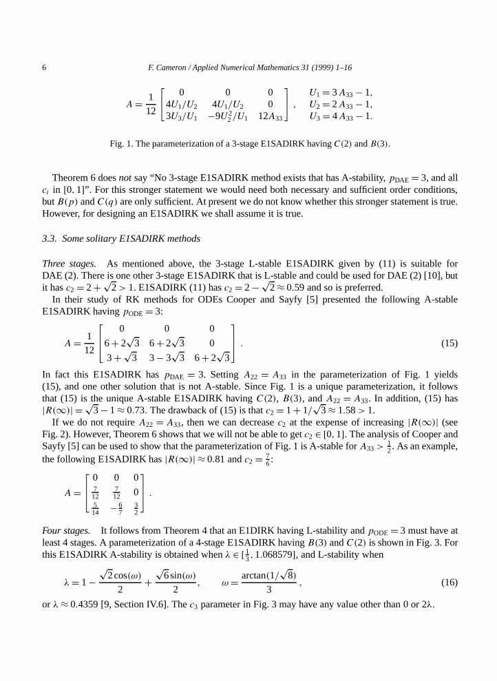
Theorem 6. No3-stage E1SADIRK exists that has A-stability,C(2), B(3), and allci in [0,1].Proof. The unique parameterization inA33 of a 3-stage E1SADIRK havingC(2) andB(3) is shown inFig. 1. Using this parameterization we get the following:

c2= 2(3A33− 1)

3(2A33− 1), (14a)

R(∞)= 6A233− 4A33+ 1

2A33(1− 3A33). (14b)

The condition|R(∞)| 6 1 impliesA33 > 1/2. To getc2 < 1 we needA33 < 1/2. These ranges forA33 do not intersect. Moreover, to getc2 = 1 we need eitherA33= 0 orA33=∞, neither of which isallowable. 2


A= 1

12

0 0 04U1/U2 4U1/U2 03U3/U1 −9U2

2/U1 12A33

, U1= 3A33− 1,U2= 2A33− 1,U3= 4A33− 1.

Fig. 1. The parameterization of a 3-stage E1SADIRK havingC(2) andB(3).

Theorem 6 doesnot say “No 3-stage E1SADIRK method exists that has A-stability,pDAE = 3, and allci in [0,1]”. For this stronger statement we would need both necessary and sufficient order conditions,butB(p) andC(q) are only sufficient. At present we do not know whether this stronger statement is true.However, for designing an E1SADIRK we shall assume it is true.

3.3. Some solitary E1SADIRK methods

Three stages. As mentioned above, the 3-stage L-stable E1SADIRK given by (11) is suitable forDAE (2). There is one other 3-stage E1SADIRK that is L-stable and could be used for DAE (2) [10], butit hasc2= 2+√2> 1. E1SADIRK (11) hasc2= 2−√2≈ 0.59 and so is preferred.

In their study of RK methods for ODEs Cooper and Sayfy [5] presented the following A-stableE1SADIRK havingpODE= 3:

A= 1

12

0 0 0

6+ 2√

3 6+ 2√

3 0

3+√3 3− 3√

3 6+ 2√

3

. (15)

In fact this E1SADIRK haspDAE = 3. SettingA22 = A33 in the parameterization of Fig. 1 yields(15), and one other solution that is not A-stable. Since Fig. 1 is a unique parameterization, it followsthat (15) is the unique A-stable E1SADIRK havingC(2), B(3), andA22= A33. In addition, (15) has|R(∞)| =√3− 1≈ 0.73. The drawback of (15) is thatc2= 1+ 1/

√3≈ 1.58> 1.

If we do not requireA22= A33, then we can decreasec2 at the expense of increasing|R(∞)| (seeFig. 2). However, Theorem 6 shows that we will not be able to getc2 ∈ [0,1]. The analysis of Cooper andSayfy [5] can be used to show that the parameterization of Fig. 1 is A-stable forA33>

12. As an example,

the following E1SADIRK has|R(∞)| ≈ 0.81 andc2= 76:

A= 0 0 0

712

712 0

514 −6

732

.Four stages. It follows from Theorem 4 that an E1DIRK having L-stability andpODE= 3 must have atleast 4 stages. A parameterization of a 4-stage E1SADIRK havingB(3) andC(2) is shown in Fig. 3. Forthis E1SADIRK A-stability is obtained whenλ ∈ [13,1.068579], and L-stability when

λ= 1−√

2cos(ω)

2+√

6sin(ω)

2, ω= arctan(1/

√8)

3, (16)

or λ≈ 0.4359 [9, Section IV.6]. Thec3 parameter in Fig. 3 may have any value other than 0 or 2λ.


Fig. 2. The compromise betweenc2 and|R(∞)| for the parameterization of Fig. 1.

0 0 0 0

λ λ 0 06c3λ− 4λ2− c2

3

4λ

c3U1

4λλ 0

12U2λ2+ 6U3λ−U3

12c3λ

6λU2+U3

12λU1

6λ2− 6λ+ 1

3c3U1λ

,

U1= c3− 2λ,

U2= 1− c3,

U3= 3c3− 2.

Fig. 3. TheA matrix for a 4-stage E1SADIRK havingC(2) andB(3).

4. Embedded E1DIRK pairs

4.1. Design objectives

In an embedded pair we have two weighting vectors,b ∈ Rs and b ∈ Rs . We refer to the two RKmethods as theb method and theb method. We use a circumflexon all items associated with theb method.

Borrowing from the discussion in Section 3.1, we can state the following design objectives for anembedded pair: (A)p andp large, (B)s small, (C) theci within the interval[0,1], and (D) all nonzeroAii the same. With regard to (A), it follows from the discussion in Section 2.3 that we will be restrictedto considering pairs of orders(3,2). Henceforth we shall assume thatp= 3 andp = 2.


We have more objectives forR(z) and R(z) than those objectives given for a solitary E1DIRK inSection 3.1. Let us consider the stable scalar test problem

y′ = µy, y(t0)= y0, µ ∈C.After taking a step of sizeh the local error of theb method is

ε1(z)≡∣∣y(t1)− y1

∣∣= ∣∣exp(z)− R(z)∣∣|y0|, (17)

wherez= hµ. The estimate of the local error after one step is

δ1(z)≡ |y1− y1| =∣∣R(z)−R(z)∣∣|y0|. (18)

Letγ ≡ ε1/δ1 be the ratio of these two errors andχ ≡ δ1/|y0| be the scaled local error estimate. We preferoverestimation of error, i.e.,γ < 1, to underestimation. However, we do not want gross overestimation,i.e., when|R(z)| ≈ 0 we do not want|R(z)−R(z)|� 0, since this will result in overly conservative stepsizes. For stiff problems we are interested in what happens when|z|→∞. Assuming we advancey withthe b method then for stiff problems we would like the following:

(i) a small|R(∞)|, so the local error (17) is small,(ii) a smallχ(z=∞), which will allow large step sizes, and(iii) γ (z=∞)≈ 1 butγ (z=∞) < 1, so the error estimate is an “accurate overestimate”.

Should we advancey with the b method then we swapR(∞) andR(∞) in (i)–(iii). Although (18)is not an estimate of local error of the higher orderb method, we still want (iii) so as to avoid bothunderestimation and gross overestimation.

Theorem 1 is the sole order result we have for designing embedded pairs for DAE (2). There are twoimportant consequences of this. The first is that our embedded pair must have twoci values equal to 1.The second consequence is that we will be designing embedded pairs for DAE (1) but not for DAE (2).The reason our embedded pairs are not suitable for (2) is that the local error ofz is proportional tohq forboth theb method and theb method (see Section 2.1).

4.2. Existence results

Three stages. As discussed above, we are restricted to designing embedded pairs having twoci equalto 1. The following result shows that we will need at least 4 stages for designing an E1SADIRK pairhaving orders(2,3) for (1).

Theorem 7. No3-stage E1SADIRK exists having the following properties: C(2), B(3), c2= c3= 1, andA real.

Proof. We use the unique parameterization shown in Fig. 1. It follows from (14a) that to getc2 = 1 weneedA33=∞, which is impermissible. 2Four stages. Unfortunately 4 stages are not enough to get a pair of orders (3,2) where both methods areL-stable:

Theorem 8. No 4-stage E1DIRK embedded pair exists with the following properties: (a) pODE = 3,(b) pODE= 2, (c)R(∞)= R(∞)= 0, and(d)A is real.

Proof. See Appendix. 2


4.3. Some E1SADIRK pairs

We will only consider 4-stage embedded pairs. We realize it will not be possible to have L-stability inboth theb method and theb method (see Theorem 8).

Two such pairs have been designed by others. Alexander and Coyle [1] derived the parameterizationof Fig. 3, but withc3= 1. They suggested using

λ= 7

12+√

13

6cos

(4π + cos−1(37

√13/169)

3

)≈ 0.4039.

The third and fourth rows ofA are thenb andb. Kværnø [12] suggested using essentially the same pairas Alexander and Coyle, but with theλ of (16). This yields an L-stableb method.

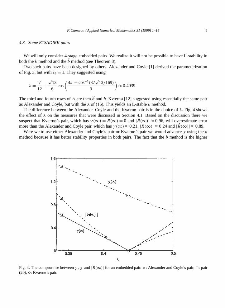
The difference between the Alexander–Coyle and the Kværnø pair is in the choice ofλ. Fig. 4 showsthe effect ofλ on the measures that were discussed in Section 4.1. Based on the discussion there wesuspect that Kværnø’s pair, which hasγ (∞)= R(∞)= 0 and|R(∞)| ≈ 0.96, will overestimate errormore than the Alexander and Coyle pair, which hasγ (∞)≈ 0.21, |R(∞)| ≈ 0.24 and|R(∞)| ≈ 0.89.

Were we to use either Alexander and Coyle’s pair or Kværnø’s pair we would advancey using thebmethod because it has better stability properties in both pairs. The fact that theb method is the higher

Fig. 4. The compromise betweenγ , χ and|R(∞)| for an embedded pair.×: Alexander and Coyle’s pair,2: pair(20),◦: Kværnø’s pair.


order method is a bonus. If L-stability is required there is an alternative: make theb method L-stable andadvancey with it. In the following pair this is the case:

A= 1

12

0 0 0 0

6+ 2√

3 6+ 2√

3 0 0

3+√3 −3√

3+ 3 6+ 2√

3 0

−√3+ 1 −5√

3− 3 4√

3+ 8 6+ 2√

3

. (19)

For this pair, the third row ofA is b and the fourth row isb. Theb method is the same as that of (15)and hence it has the same properties: A-stability and|R(∞)| ≈ 0.73. The drawback of this pair is againthe largec2 value: c2 ≈ 1.58. We did not try to reducec2 by letting theAii values differ as we did inSection 3.3.

We can form two other E1SADIRK pairs where thebmethod is L-stable using the parameterization ofFig. 3 withc3= 1. These two pairs are obtained by settingλ= 1±1/

√2. Unfortunately, as Kværnø [12]

notes both pairs have serious drawbacks: for one pairc2≈ 3.41 and for the other pair|R(∞)| ≈ 1.61.We present one more pair. For this pair we start with the parameterization of Fig. 3 and we setc3= 1

andλ= 1750:

A=

0 0 0 01750

1750 0 0

361850

417

1750 0

1351

625816 − 433

12001750

. (20)

We consider (20) not because it was designed using objectives presented here, but rather because itexhibited an interesting phenomenon in the tests. For pair (20)|R(∞)| ≈ 0.91, |R(∞)| ≈ 0.56 andγ (∞)≈ 0.62.

5. Tests

5.1. Implementation details

We tested four different E1SADIRK pairs: (i) (19), (ii) (20), (iii) the pair suggested by Alexanderand Coyle, and (iv) the pair suggested by Kværnø. These last two pairs are described at the start ofSection 4.3; we will refer to them as the AC pair and the Kv pair. For all except pair (i) we advancedy

using the higher orderb method.For all four pairs each step requires solving three non-linear equation sets, one for each implicit stage.

In our Newton process we used the same Jacobian matrixJ for all implicit stages;J was computed at thestart of each step. Let1Y(k) be thekth Newton increment for stage variableY . The slowest convergencerate during the Newton process is

αmax=maxk

‖1Y(k)‖‖1Y(k− 1)‖ , k = 2,3, . . . , kmax.


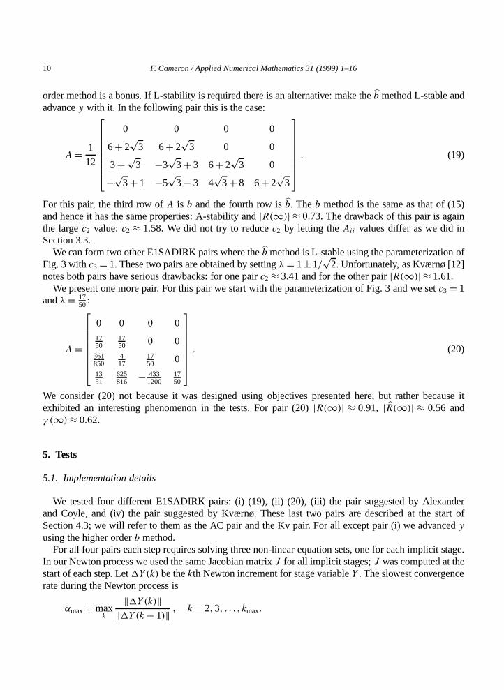
begin1. Solve forα∗: αkmax−ksafe∗ /(1− α∗) = κNewt‖β‖/maxk ‖1Y(k)‖2. hNewt= α∗hold/αmax

3. if in the most recent RK step Newton convergence failedthen4. hnew= hNewt

5. else6. εi = |yi − yi |/βi, i = 1,2, . . . ,N7. ν = (2kmax+ 1)/(2kmax+ kmost)

8. hRK = κRKνhold/‖ε‖1/39. hnew=min(hNewt, hRK)

10. if ‖ε‖< 1 then accept the most recent RK step11. elsereject the most recent RK step12. endif13. endif

exit

Fig. 5. The step-size controller.

Newton iterations are stopped ifαmax> 1 or if kmax iterations are taken without satisfying the convergencecriterion, which is given below. Givenyn, the initial value fed to the Newton process for stagei wascomputed as follows:

Yi(0)=yn, if ci >max(cj , j = 1, . . . , i − 1),[(ci − c`)Yj + (ci − cj )Y`]

(cj − c`) , if ci ∈ [c`, cj ], c` 6= cj , j, ` < i.

In our step-size controller and Newton convergence criterion we have used ideas from [9, Section IV.8]and [7, Chapter 5]. Some of the parameters of the controller (Fig. 5) require explanation. Theβ vectorspecifies the tolerance we require:

βi = νi + r|yi |, (21)

whereyi is representative of the current value ofyi , r is the relative tolerance andνi is the threshold foryi . ThehNewt value is meant to ensure that the Newton process converges inkmax− ksafe iterations in thenext attempted RK step. Lettingk` be the number of Newton iterations taken in stage` in the step justattempted, thenkmost=max(k2, k3, k4). TheκNewt parameter is meant to ensure that the error remainingafter Newton convergence is insignificant compared to the RK truncation error. Newton convergence isattained ifk 6 kmax and

αmax

1− αmax6 κNewt‖β‖‖1Y(k)‖ . (22)

In all tests we used the following values:kmax= 10, ksafe= 2, κNewt = 0.001, κRK = 0.8, andν` =r/1000, `= 1,2, . . . ,N .

When applied to (1) whereS depends ony, E1RK methods are not self-starting. In other words, forthe first step eithery′(t0) must be provided, or a different method must be used. We assumed the former.

All tests were performed in MATLAB on a Digital AlphaStation computer.


5.2. Results

We used the following DAE system for our tests:0

√y2 2y2

4y1√y2 0 −2

√y2

4y1√y2 0 −2

√y2

y′1y′2y′3

=

4y2y1(2y1− y3−√y2 )

τ(2− y2)+ y12−√2− e−τ t + 1− y3

τe−τ t

. (23)

This system has the following solution:y1(t)= (t + 1)/(t + 2), y2(t) = 2− e−τ t , andy3(t)= y21(t)−√

y2(t)+ 1. We used twoτ values: (A)τ = 2, and (B)τ = 500. For (B) the DAE test system (23) hasdynamics that are clearly of different orders of magnitude, i.e., it is stiff.

We measured global error using

ErrG=max`

(maxi

(∣∣yi(t`)− yi,`∣∣)),whereyi,` is the RK estimate ofyi at t`. The target final time wastf = 1.5. Our work measure was theCPU time estimated by MATLAB. This work measure does not take into account the amount by whichsome pair overshootstf . We generated our results by changing the relative tolerancer in (21).

Fig. 6 contains the results forτ = 2. Pair (19) is clearly set off from the other pairs. For this simulationwe conclude that the advantage of advancingy with the higher orderb method is that we get at leasttwo orders of magnitude more accuracy for the same CPU time. Amongst the other three pairs there is

Fig. 6. Simulation A,τ = 2.∗: pair (19),×: Alexander and Coyle’s pair,2: pair (20),◦: Kværnø’s pair.


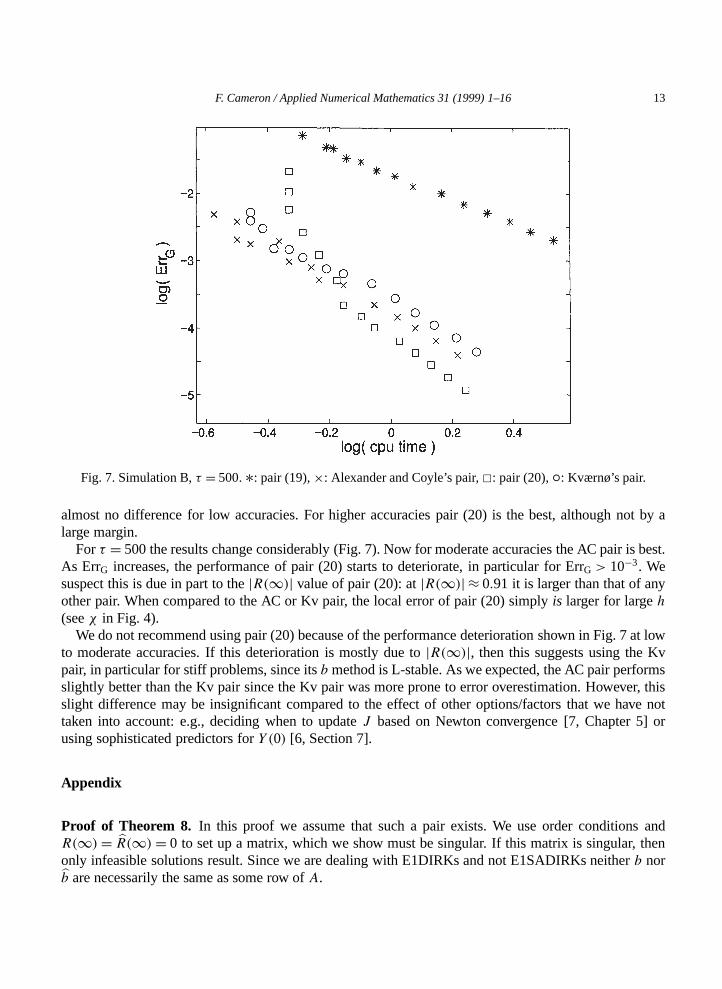
Fig. 7. Simulation B,τ = 500.∗: pair (19),×: Alexander and Coyle’s pair,2: pair (20),◦: Kværnø’s pair.

almost no difference for low accuracies. For higher accuracies pair (20) is the best, although not by alarge margin.

Forτ = 500 the results change considerably (Fig. 7). Now for moderate accuracies the AC pair is best.As ErrG increases, the performance of pair (20) starts to deteriorate, in particular for ErrG > 10−3. Wesuspect this is due in part to the|R(∞)| value of pair (20): at|R(∞)| ≈ 0.91 it is larger than that of anyother pair. When compared to the AC or Kv pair, the local error of pair (20) simplyis larger for largeh(seeχ in Fig. 4).

We do not recommend using pair (20) because of the performance deterioration shown in Fig. 7 at lowto moderate accuracies. If this deterioration is mostly due to|R(∞)|, then this suggests using the Kvpair, in particular for stiff problems, since itsb method is L-stable. As we expected, the AC pair performsslightly better than the Kv pair since the Kv pair was more prone to error overestimation. However, thisslight difference may be insignificant compared to the effect of other options/factors that we have nottaken into account: e.g., deciding when to updateJ based on Newton convergence [7, Chapter 5] orusing sophisticated predictors forY (0) [6, Section 7].

Appendix

Proof of Theorem 8. In this proof we assume that such a pair exists. We use order conditions andR(∞)= R(∞)= 0 to set up a matrix, which we show must be singular. If this matrix is singular, thenonly infeasible solutions result. Since we are dealing with E1DIRKs and not E1SADIRKs neitherb norb are necessarily the same as some row ofA.


We use the following parameterization:

A=

0 0 0 0

c2 A22 0 0

c3−A32−A33 A32 A33 0

c4−A42−A43−A44 A42 A43 A44

.

The denominator of eitherR(z) or R(z) is given by4∑i=0

hizi = 1− (A22+A33+A44)z+ (A22A33+A22A44+A33A44)z

2−A22A33A44z3. (24)

To attainR(∞)= 0 we needg4= g3= 0 (see (12)). Using (13),h0= 1, and order conditions (7) and (8)we can write

g3= h3+ h2+ 12h1+ bTAc = 0. (25)

In a similar fashion we can expressg4 as

g4= h3+ 12h2+ h1b

TAc+ bTA2c= 0. (26)

We can combine (25) and (26) with order conditions (7) and (8) to obtain

bT[ e c Ac A2c]= [1 1

2 − h3− h2− 12h1 h3(h1− 1)+ h2

(h1− 1

2

)+ 12h

21

]. (27)

We can get the same expression as (27) for theb method since it satisfies (7), (8), andg4 = g3 = 0. Itfollows that(

bT − bT)[ e c Ac A2c]= [0 0 0 0]. (28)

Since we wantb 6= b, it follows thatM = [e c Ac A2c] must be singular. Since the first row ofA hasonly zeros andc1= 0, it follows that

δ1c= δ2Ac+ δ3A2c. (29)

There are four cases to consider: (a)δ1= 1, δ2 6= 0, δ3 6= 0, (b) δ1= 1, δ2 6= 0, δ3= 0, (c) δ1= 1, δ2= 0,δ3 6= 0, and (d)δ1= 0, δ2= 1, δ3 6= 0.

Case(a). Eq. (29) has three solutions, all having the form

[δ2 δ3] = (AiiAjj )−1[(Aii +Ajj ) −1]. (30)

The solutions have[i, j ] equal to[2,3], [2,4], and[3,4]. We use (29) in (26) to get

h3+ h2/2+ h1bTAc+ δ−1

3 bT(c− δ2Ac)= 0.

Since we have assumedpODE= 3, we can use (10) and (8) in this expression to get

h3+ 12h2+ 1

6h1+ δ−13

(12 − 1

6δ2)= 0.

Into this expression we substitute (30) and the coefficients from (24) to get

−A22A33A44+ 12A33A44+ 1

2A22A44+ 12A22A33− 1

6A44− 16A33− 1

6A22

− 12AiiAjj + 1

6Aii + 16Ajj = 0. (31)


Using (10) and the coefficients from (24) in (25) yields

A22A33A44−A33A44−A22A44−A22A33+ 12A44+ 1

2A33+ 12A22= 1

6. (32)

When considering (31) and (32) we have three cases to consider: the three solutions of (30). However,owing to the symmetry of the expressions with respect toA22, A33, andA44, all three cases yield similarconclusions. For example, using[i, j ] = [2,3] in (31) results in

A44(6A22A33− 3A33− 3A22+ 1)= 0. (33)

All solutions of (33) and (32) have eitherA44= 0, or complex values forA22 andA33. Neither of theseis permissible.

Case(b). For this case (29) has three solutions:δ2=A−1ii , for i = 2,3, or 4. UsingAii c=Ac and (8)

in order condition (10) yields16 = bTAc =AiibTc= 1

2Aii

or Aii = 13. The dependenceAiic = Ac implies A2

iic = A2c. Using these dependencies and thecoefficients from (24) in (26) yields

−A22A33A44+ 12(A33A44+A22A44+A22A33)− 1

2Aii(A22+A33+A44)+ 12A

2ii = 0. (34)

In principle we have three solutions to test in (34)—Aii = 13, i = 2,3,4. Because of symmetry all three

solutions yield the impermissible result thatAjj = 0 for somej 6= i. For example, usingAii =A22= 13

in (34) yields16A33A44= 0.

Cases(c) and (d) yield the same result as Case (b). To see this, we letA be the lower right diagonal3×3 block ofA, andc= [c2 c3 c4]T. Note thatA is invertible. Since the first row ofA has only zeros andc1= 0, it follows that the singularity of[e c Ac A2c] of (28) is equivalent to the singularity of[c Ac A2c].Hence (29) is valid whenA andc are replaced byA and c. Cases (b)–(d) all correspond toc being aneigenvector ofA. Whenc is an eigenvector it follows thatc=A−1

ii Ac=A−2ii A

2c. 2References

[1] R. Alexander and J.J. Coyle, Runge–Kutta methods and differential algebraic systems,SIAM J. Numer. Anal.27 (1990) 736–752.

[2] K.E. Brenan, S.L. Campbell and L.R. Petzold,Numerical Solution of Initial-Value Problems in Differential–Algebraic Equations(SIAM, Philadelphia, PA, 1996).

[3] F. Cameron, On low order DIRKs and DAEs, submitted (1998).[4] F. Cameron, R. Piché and K. Forsman, Variable step size time integration methods for transient eddy current

problems,IEEE Trans. Magn.(1998, in press).[5] G.J. Cooper and A. Sayfy, Semiexplicit A-stable Runge–Kutta methods,Math. Comp.33 (1979) 541–556.[6] J.J.B. de Swart, W.M. Lioen and W.A. van der Veen, Specification of PSIDE (1997), available at

http://www.cwi.nl/cwi/projects/PSIDE/ .[7] K. Gustafsson, Control of error and convergence in ODE solvers, Ph.D. Thesis, Lund Institute of Technology

(1992).[8] E. Hairer, C. Lubich and M. Roche,The Numerical Solution of Differential–Algebraic Systems by Runge–

Kutta Methods, Lecture Notes in Mathematics, Vol. 1409 (Springer, Berlin, 1989).[9] E. Hairer and G. Wanner,Solving Ordinary Differential Equations, Vol. 2: Stiff and Differential–Algebraic

Problems(Springer, Berlin, 1991).


[10] M. Hosea and L. Shampine, Analysis and implementation of TR-BDF2,Appl. Numer. Math.20 (1996) 21–37.[11] L. Jay, Convergence of a class of Runge–Kutta methods for differential algebraic systems of index 2,BIT 33

(1993) 137–150.[12] A. Kværnø, More and, to be hoped, better DIRK methods for the solution of stiff ODEs, Unpublished

manuscript, Department of Mathematical Sciences, Norwegian University of Science and Technology,Trondheim (1992).

[13] C. Lubich, Linearly implicit extrapolation methods for differential–algebraic systems,Numer. Math.55 (1989)197–211.

[14] D.M. Wiberg,Theory and Problems of State Space and Linear Systems, Schaum’s Outline Series (McGraw-Hill, New York, 1971).

A class of low order DIRK methods for a class of DAEs

Documents

Transcript of A class of low order DIRK methods for a class of DAEs