A class of geostatistical methods to predict and simulate ...
89
POLITECNICO DI MILANO Corso di Laurea Magistrale in Ingegneria Matematica Scuola di Ingegneria Industriale e dell’Informazione A class of geostatistical methods to predict and simulate seismic ground motion fields: from a univariate to a functional approach Supervisor: Dr. Alessandra Menafoglio Co-supervisor: Dr. Sara Sgobba Tesi di Laurea di: Filippo Lentoni Matricola 878653 Anno Accademico 2017-2018
Transcript of A class of geostatistical methods to predict and simulate ...

POLITECNICO DI MILANOCorso di Laurea Magistrale in Ingegneria MatematicaScuola di Ingegneria Industriale e dell’Informazione
A class of geostatistical methods to
predict and simulate seismic ground
motion fields: from a univariate to a
functional approach
Supervisor: Dr. Alessandra MenafoglioCo-supervisor: Dr. Sara Sgobba
Tesi di Laurea di:Filippo Lentoni
Matricola 878653
Anno Accademico 2017-2018

1

Abstract
Earthquakes have been constantly studied due to their devastating effects interms of loss of human life and economic damages. In order to limit these effectsand investigate the nature of this phenomenon, in literature, the generation ofshaking fields has been proposed based on empirical models which predict theground motion (Ground Motion Prediction Equation, GMPE). The variance re-lated to the prediction error of these models and the spatial covariance of theirresiduals have been also studied, with the purpose of understanding if GMPEsare able to describe exhaustively the phenomenon and finding the possible correc-tive terms. Thanks to several records of waveforms collected during the seismicsequence of Emilia in 2012, it was possible to model the prediction error of aGMPE specific for the Northern part of Italy with a fully non-ergodic approachwhich identifies a systematic corrective term in the residuals for the median pre-diction of the model.The aim of this thesis is to build shaking fields through the combination of theprediction of the aforementioned GMPE, the prediction and the simulation ofits corrective term and of its residual uncertainty with both the univariate andthe functional approaches to the geostatistics. The application of this last ap-proach to Applied Seismology is innovative and allows to provide predictions andjoint stochastic simulations of many intensity measures through computationaland modeling efforts comparable to the ones of the multivariate approach. Thethesis shows that for some relevant intensity measures the performances of thefunctional approach on the predictions are comparable or better than the ones ofthe univariate approach, thus providing more complete and more robust results.

Sommario
I terremoti sono da sempre oggetto di studio per via degli effetti devastanti cheprovocano in termini di perdite di vite umane e danni di natura economica. Alfine di limitare tali effetti e studiare la natura di questi fenomeni, in lettera-tura e stata proposta la generazione di mappe di scuotimento del suolo basatesu modelli empirici predittivi del moto del terreno (Ground Motion PredictionEquation, GMPE). Sono inoltre state indagate la varianza associata all’errore dipredizione di tali modelli e la covarianza spaziale dei relativi residui con lo scopodi capire se le equazioni GMPE descrivano esaustivamente il fenomeno e di stu-diarne eventuali termini correttivi. Le molteplici registrazioni di forme d’ondaeffettuate nella sequenza dell’Emilia nel 2012 hanno permesso la modellizzazionedell’errore di predizione di una GMPE specifica per il Nord Italia con un ap-proccio pienamente non ergodico, che individua nei residui della regressione untermine sistematico correttivo della predizione mediana del modello GMPE.L’obiettivo della tesi e realizzare mappe di scuotimento tramite la combinazionedi tre elementi: la predizione della sopraccitata GMPE, la predizione e la simu-lazione del suo termine correttivo e dell’incertezza residua ad esso associata, conun approccio dapprima univariato quindi funzionale alla geostatistica. L’appli-cazione di metodi di analisi funzionale alla sismologia applicata e innovativo econsente di fornire previsioni e simulazioni stocastiche congiunte di molteplicimisure d’intensita con uno sforzo modellistico e computazionale comparabile aquello del caso multivariato. La tesi mostra che le performance dell’approcciofunzionale sulla previsione di alcune misure d’intensita rilevanti sono comparabilio migliori dell’approccio univariato, fornendo quindi risultati piu completi e piurobusti.

2

Contents
Sommario 1
Introduction 11
1 State Of The Art 13
1.1 PGA and SA . . . . . . . . . . . . . . . . . . . . . . . . . . . . . 13
1.2 Ground Motion Models (GMM) . . . . . . . . . . . . . . . . . . . 14
1.3 Ergodic And Non-ergodic Assumptions . . . . . . . . . . . . . . . 15
1.4 Modelling the spatial dependence among residuals . . . . . . . . 18
2 Study Framework and Dataset 19
2.1 Study Area . . . . . . . . . . . . . . . . . . . . . . . . . . . . . . 19
2.2 Ground Motion Prediction Equation . . . . . . . . . . . . . . . . 22
2.3 Dataset . . . . . . . . . . . . . . . . . . . . . . . . . . . . . . . . 24
3 A univariate approach to the geostatistical analysis of intensitymeasures 27
3.1 Modelling the Covariance of the Random Field . . . . . . . . . . 27
3.1.1 Drift Estimation . . . . . . . . . . . . . . . . . . . . . . . 29
3.1.2 Geostatistical analysis of the corrective term and σ0,sr . . 30
3.1.3 Analysis of corrective term . . . . . . . . . . . . . . . . . 31
3.1.4 Analysis of σ0,sr . . . . . . . . . . . . . . . . . . . . . . . 36
3.2 Kriging . . . . . . . . . . . . . . . . . . . . . . . . . . . . . . . . 39
3.2.1 Introduction . . . . . . . . . . . . . . . . . . . . . . . . . 39
3.2.2 Kriging for the corrective terms . . . . . . . . . . . . . . . 40
3.2.3 Kriging for σ0,sr . . . . . . . . . . . . . . . . . . . . . . . 43
3.3 Conditional Simulation . . . . . . . . . . . . . . . . . . . . . . . . 44
3.3.1 Introduction . . . . . . . . . . . . . . . . . . . . . . . . . 44
3.3.2 Sequential simulation for corrective term . . . . . . . . . . 46
3.3.3 Sequential simulation for σ0,sr . . . . . . . . . . . . . . . . 48
3.3.4 Comparison of different periods in the faults zone . . . . . 51
4 Functional geostatistics for the joint analysis of intensity mea-sures over a range of periods 53
4.1 State Of The Art . . . . . . . . . . . . . . . . . . . . . . . . . . . 53
4.2 Functional Data Analysis . . . . . . . . . . . . . . . . . . . . . . 54
3

4 CONTENTS
4.2.1 Introduction . . . . . . . . . . . . . . . . . . . . . . . . . 544.2.2 Representing functions by basis functions . . . . . . . . . 544.2.3 Spline functions . . . . . . . . . . . . . . . . . . . . . . . . 554.2.4 The B-spline basis for spline functions . . . . . . . . . . . 554.2.5 Smoothing Functional Data By Least Squares . . . . . . . 554.2.6 Smooting functional data with a roughness penality . . . 564.2.7 Roughness . . . . . . . . . . . . . . . . . . . . . . . . . . . 56
4.3 Application to data . . . . . . . . . . . . . . . . . . . . . . . . . . 574.4 Principal Component Analysis . . . . . . . . . . . . . . . . . . . 62
4.4.1 PCA for multivariate data . . . . . . . . . . . . . . . . . . 624.4.2 Defining PCA for functional data . . . . . . . . . . . . . . 634.4.3 Eigenanalysis . . . . . . . . . . . . . . . . . . . . . . . . . 64
4.5 PCA Application . . . . . . . . . . . . . . . . . . . . . . . . . . . 654.6 Multivariate Sequential Simulation . . . . . . . . . . . . . . . . . 72
4.6.1 Application for Correttive Term and σ0,sr . . . . . . . . . 73
5 Model validation and testing 775.1 Model Comparison . . . . . . . . . . . . . . . . . . . . . . . . . . 775.2 Test . . . . . . . . . . . . . . . . . . . . . . . . . . . . . . . . . . 78
6 Conclusion 81
Bibliography 83

List of Figures
1.1 Single degree of freedom system. . . . . . . . . . . . . . . . . . . 13
2.1 Stations, fault and epicenters. . . . . . . . . . . . . . . . . . . . . 20
2.2 Location of the geological cross-section(red) and the northernApennines frontal thrust(yellow). . . . . . . . . . . . . . . . . . 21
2.3 Surface waves generation (Paolucci et al.,2015). . . . . . . . . . . 21
2.4 Stations and ZS912(red). . . . . . . . . . . . . . . . . . . . . . . . 25
3.1 Distribution of stations. . . . . . . . . . . . . . . . . . . . . . . . 30
3.2 Bubbleplot PGA. . . . . . . . . . . . . . . . . . . . . . . . . . . . 31
3.3 Directional variograms. . . . . . . . . . . . . . . . . . . . . . . . . 31
3.4 Sample variogram. . . . . . . . . . . . . . . . . . . . . . . . . . . 32
3.5 fitted variogram. . . . . . . . . . . . . . . . . . . . . . . . . . . . 33
3.6 Bubbleplot for corrective term at T = 4s. . . . . . . . . . . . . . 33
3.7 Directional variograms. . . . . . . . . . . . . . . . . . . . . . . . . 34
3.8 Sample variogram fitted. . . . . . . . . . . . . . . . . . . . . . . . 34
3.9 Residual variogram. . . . . . . . . . . . . . . . . . . . . . . . . . 35
3.10 Comparison of correlation coefficients. . . . . . . . . . . . . . . . 36
3.11 Bubbleplot and directional variogram PGA. . . . . . . . . . . . . 37
3.12 Bubbleplot and directional variogram T = 4s. . . . . . . . . . . . 37
3.13 Variogram of PGA and on the left and variogram of SA(T = 4)on the right fitted with the exponential model. . . . . . . . . . . 38
3.14 Comparison of correlation coefficients of PGA and SA(T = 4s). . 39
3.15 Ordinary kriging prediction and variance for PGA. . . . . . . . . 40
3.16 Ordinary kriging prediction in the fault zone. The colour scalehas been modified to highlight local differences. . . . . . . . . . 41
3.17 Drift for corrective term (left panel) and simple kriging predictionof the residuals (right panel). . . . . . . . . . . . . . . . . . . . . 41
3.18 Universal kriging prediction and variance of corrective term atT = 4s. . . . . . . . . . . . . . . . . . . . . . . . . . . . . . . . . 42
3.19 Universal kriging prediction (zoom). The colour scale has beenmodified to highlight local differences. . . . . . . . . . . . . . . . 42
3.20 Ordinary kriging prediction and variance for the PGA. . . . . . . 43
3.21 Ordinary kriging prediction and variance of SA(T = 4s). . . . . . 43
5

6 LIST OF FIGURES
3.22 Ordinary kriging prediction of PGA and SA(T = 4s), zoom onthe faults. The colour scale has been modified to highlight localdifferences. . . . . . . . . . . . . . . . . . . . . . . . . . . . . . . 44
3.23 The kriging prediction and the conditional simulation for PGA. . 46
3.24 The kriging prediction and the conditional simulation, faults zonefor PGA. The colour scale has been modified to highlight localdifferences. . . . . . . . . . . . . . . . . . . . . . . . . . . . . . . 47
3.25 Comparison between the average scenario and the simulation T=4s. 47
3.26 The kriging prediction and the conditional simulations for SA(T=4s),faults zone. The colour scale has been modified to highlight localdifferences. . . . . . . . . . . . . . . . . . . . . . . . . . . . . . . 48
3.27 The kriging prediction and the conditional simulation. . . . . . . 49
3.28 The kriging prediction and the conditional simulation, faults zone.The colour scale has been modified to highlight local differences. 49
3.29 The kriging prediction and the conditional simulation. . . . . . . 50
3.30 The kriging prediction and the conditional simulation, faults zone.The colour scale has been modified to highlight local differences. 50
3.31 Comparison of conditional simulation, corrective term, PGA inleft panel and Sigma SA(T=4s) in the right panel. . . . . . . . . 51
3.32 Comparison of conditional simulation, σ0,sr PGA in left panel andσ0,sr SA(T=4s) in the right panel. . . . . . . . . . . . . . . . . . 51
4.1 The original corrective terms at different periods, for differentstations. . . . . . . . . . . . . . . . . . . . . . . . . . . . . . . . . 57
4.2 B-spline basis. . . . . . . . . . . . . . . . . . . . . . . . . . . . . . 58
4.3 Stations located in the Appenninic Area and in the faults zone. . 59
4.4 Smoothing spline for Stations SAG0 and SMS0. . . . . . . . . . . 59
4.5 Smoothing spline for stations BON0 and SAN0. . . . . . . . . . . 59
4.6 Smoothing spline for stations FICO,FAZ. . . . . . . . . . . . . . 60
4.7 Smoothing spline for stations MOLI,MDC . . . . . . . . . . . . . 60
4.8 Original data on the left and on the right the smoothing splines. 61
4.9 Original data on the left and on the right the smoothing splines. 61
4.10 Smoothing spline for Stations SAG0 and SMS0 (σ0,sr). . . . . . . 61
4.11 Smoothing spline for Stations BON0,SAN0 (σ0,sr). . . . . . . . . 62
4.12 Smoothing spline for Stations FICO, FAZ (σ0,sr). . . . . . . . . . 62
4.13 Smoothing spline for Stations MOLI, MDC (σ0,sr). . . . . . . . . 62
4.14 Principal Component curves for corrective term. . . . . . . . . . 65
4.15 Cumulative variance. . . . . . . . . . . . . . . . . . . . . . . . . . 66
4.16 Boxplot of scores. . . . . . . . . . . . . . . . . . . . . . . . . . . . 66
4.17 Smoothing spline projected on different spaces. . . . . . . . . . . 67
4.18 Smoothing spline projected on different spaces. . . . . . . . . . . 67
4.19 Smoothing spline projection for stations SAG0 and SMS0. . . . 68
4.20 Smoothing spline projection for station BON0 and SAN0. . . . . 68
4.21 Smoothing spline projection for stations FIC0 and FAZ. . . . . . 68
4.22 Smoothing spline projection for stations IMOL and MDC. . . . 68
4.23 Principal Component curves for corrective term. . . . . . . . . . 69

LIST OF FIGURES 7
4.24 Cumulative variance . . . . . . . . . . . . . . . . . . . . . . . . . 694.25 Boxplot of scores . . . . . . . . . . . . . . . . . . . . . . . . . . . 704.26 Original smoothing spline and smoothing spline projected. . . . . 704.27 Smoothing spline projection for stations located in the faults zone. 714.28 Smoothing spline projection for stations BON0 and SAN0 . . . . 714.29 Smoothing spline projection for stations FIC0 and FAZ . . . . . 714.30 Smoothing spline projection for stations IMOL and MDC . . . . 714.31 Corrective term(on the left) and σ0,sr (on the right) variograms
and cross-variograms fitted with the exponential model. . . . . . 734.32 Sequential simulation of corrective term PGA(on the left) and
T = 4s (on the right). . . . . . . . . . . . . . . . . . . . . . . . . 744.33 Sequential simulation of corrective term PGA (on the left) and
T = 4s (on the right), zoom on the faults. . . . . . . . . . . . . . 744.34 Sequential simulation of σ0,sr PGA (on the left) and T = 4s (on
the right). . . . . . . . . . . . . . . . . . . . . . . . . . . . . . . . 754.35 Sequential simulation of σ0,sr PGA (on the left) and T = 4s (on
the right), zoom on the faults. . . . . . . . . . . . . . . . . . . . . 75
5.1 Shaking fields for PGA and SA(T=4s). . . . . . . . . . . . . . . . 805.2 GMPE and shaking field for PGA, same scale. . . . . . . . . . . 805.3 GMPE and shaking field for SA(T=4s), same scale. . . . . . . . . 80

8 LIST OF FIGURES

List of Tables
2.1 Features of 1st and 2nd Emilia earthquake. ML is the Ricthermagnitude and MW is the moment magnitude. . . . . . . . . . . 19
3.1 Model Comparison. . . . . . . . . . . . . . . . . . . . . . . . . . . 323.2 Exponential model parameters. . . . . . . . . . . . . . . . . . . . 323.3 Model Comparison. . . . . . . . . . . . . . . . . . . . . . . . . . . 353.4 Exponential model parameters. . . . . . . . . . . . . . . . . . . . 363.5 Model Comparison PGA. . . . . . . . . . . . . . . . . . . . . . . 373.6 Model Comparison SA(T = 4s). . . . . . . . . . . . . . . . . . . . 383.7 Exponential model parameters PGA. . . . . . . . . . . . . . . . . 383.8 Exponential model parameters SA(T = 4s). . . . . . . . . . . . . 38
5.1 Univariate geostatistics performances, MSE. . . . . . . . . . . . . 775.2 Univariate geostatistics performances, VAR . . . . . . . . . . . . 775.3 Functional geostatisctics performances, MSE. . . . . . . . . . . . 785.4 Functional geostatistics performances, VAR. . . . . . . . . . . . . 785.5 MSE for the model (univariate) and GMPE at PGA. . . . . . . 795.6 MSE for the model (functional) and GMPE at PGA. . . . . . . . 795.7 MSE for the model(functional) and for the GMPE at T = 4s. . . 79
9

10 LIST OF TABLES

Introduction
How much does it cost to save a human life through the seismic adaptation ofexisting buildings? What are the factors that most significantly influence theseismic motion? With which criteria can the seismic hazard of a region or a sitebe measured? What is the probability that the peak ground acceleration exceedsa certain intensity? These are just some of the big queries that seismology triesto answer.The prediction of ground acceleration when an earthquake occurs is essential toanswer such questions. The probability of exceeding a certain level of groundmotion for a given earthquake scenario is generally computed through the useof Ground Motion Prediction Equations (GMPE). These prediction models arelinear regression models whose accuracy increases if the features used (e.g. mag-nitude, distance from the epicenter, etc.) are the most suitable to describe thephenomenon.Earthquakes are very complex phenomena to be modeled and a linear predic-tion model is often unable to capture all the complex interactions between wavepropagation and the path in which it propagates, resulting in a high variance ofprediction error.In order to take into account these complex interactions, a further analysis ofprediction residuals must be developed to identify the presence of systematicand repeatable contributions that correct the prediction. If the new prediction,given by the sum of the model and the corrective term, has a lower predictionerror, it means that an additional deterministic component of the phenomenonhas been identified.A non-ergodic approach is the most effective for determining the corrective termbut it is applicable to residuals only when a large number of seismic recordings isavailable. Using this approach, the Istituto Nazionale di Geofisica e Vulcanolo-gia (INGV) has calculated the corrective term and the variance of the residualsrelated to the spectral acceleration for different natural periods of oscillation.This quantity allows to compute and model the seismic action for structuralresponse assessment. Since the residuals and the remaining aleatory variabilityare provided with coordinates, their spatial correlation has been investigated inorder to highlight differences in the behavior at low and high periods and predicttheir value in new positions of the space. For this purpose, it has been adoptedthe univariate approach to geostatistics that models the spatial covariance of thecorrective term considering each period independently.The corrective term is modelled as the sum of a deterministic term and a ran-
11

12 INTRODUCTION
dom one. Variograms have been used to find the spatial covariance while theprediction has been computed through ordinary kriging, in case the determinis-tic part is constant in the space, or universal kriging when the deterministic partdepends on the spatial coordinates (Cressie 1993). In order to consider the vari-ance related to these predictions, Gaussian sequential simulation has been used.It enables to simulate a new value of the spectral acceleration taking into accountthe correlation with the values already simulated. To take into account also thecorrelation between the different spectral periods, multivariate geostatistics canbe applied (Chiles et Delfiner, 1999).However, it presents some limits such as the possibility to compute a restrictednumber of spectral periods simultaneously.In this study, in order to overcame the aforementioned limit, for the first timea functional geostatistics approach has been implemented in applied seismologyto study the corrective term of the GMPE and the related variance at differentperiods jointly. This approach is motivated by the fact that the spectral accel-eration is a function of the natural period of oscillation of the building. Thisapproach combines Functional Data Analysis (FDA, Ramsay and Silverman,2005) techniques with the ones of multivariate geostatistics. Indeed, FDA allowsto approximate a collection of discreet observations through a smooth functionand to project these on a new reference system whose basis is made of the mainprincipal directions (i.e. Functional Principal Components). In this way, thefunction is represented through a vector of coordinates representing the functionin the new reference system.Instead, the geostatistics multivariate approach, by means of the cokriking, al-lows us to predict the vector of coordinates in new positions of the space andthus to create the complete curve of both the corrective terms and the variancethrough the linear combination of the functions of the basis.The application of the Functional Geostatistics approach to Applied Seismol-ogy is a turning point since it allows to provide predictions and joint stochasticsimulations of all the periods by means of computational and modeling effortscomparable to the ones of the multivariate approach.The thesis is organized as follows: Chapter 1 presents a review of literatureregarding the GMPE and the ergodic assumption. Chapter 2 describes the case-study and the dataset. Chapter 3 describes the univariate approach to thegeostatistical analysis of intensity measures. Chapter 4 describes the Functionalgeostatistics approach. Chapter 5 shows models comparison and the results.

Chapter 1
State Of The Art
The aim of this Chapter is first to introduce the reader to the key conceptsof seismology and engineering seismology we have employed in the thesis andsecondly to explain how the previous studies have inspired us and what are theinnovations of our analysis in comparison to the other ones.
1.1 PGA and SA
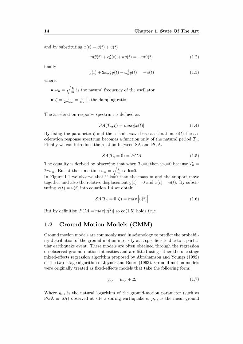
The peak ground acceleration (PGA), in a specific location, is defined as the am-plitude of the largest peak acceleration recorded by a local accelerogram duringan earthquake (Douglas 2003).In order to introduce the acceleration response spectrum (SA), we need to de-scribe the dynamic equation of a Single Degree Of Freedom System (SDOF).The SDOF is made up of a mass m, a spring with stiffness k and a dashpot witha coefficient of viscous damping c.
Figure 1.1: Single degree of freedom system.
Let u(t) be the absolute displacement of the support at time t, x(t) the absolutedisplacement of the oscillator and y(t) := x(t) − u(t) the relative displacementof the oscillator with respect to support.Then using Newton’s second law we obtain the dynamic equilibrium equation:
mx(t) + cy(t) + ky(t) = 0 (1.1)
13
14 Chapter 1. State Of The Art
and by substituting x(t) = y(t) + u(t)
my(t) + cy(t) + ky(t) = −mu(t) (1.2)
finallyy(t) + 2ωnζy(t) + ω2
ny(t) = −u(t) (1.3)
where:
• ωn =√
km is the natural frequency of the oscillator
• ζ = c2mωn
= cccr
is the damping ratio
The acceleration response spectrum is defined as:
SA(Tn, ζ) = maxt|x(t)| (1.4)
By fixing the parameter ζ and the seismic wave base acceleration, u(t) the ac-celeration response spectrum becomes a function only of the natural period Tn.Finally we can introduce the relation between SA and PGA.
SA(Tn = 0) = PGA (1.5)
The equality is derived by observing that when Tn=0 then wn=0 because Tn =
2πwn. But at the same time wn =√
km so k=0.
In Figure 1.1 we observe that if k=0 than the mass m and the support movetogether and also the relative displacement y(t) = 0 and x(t) = u(t). By substi-tuting x(t) = u(t) into equation 1.4 we obtain
SA(Tn = 0, ζ) = max∣∣∣ ¨u(t)
∣∣∣ (1.6)
But by definition PGA = max| ¨u(t)| so eq(1.5) holds true.
1.2 Ground Motion Models (GMM)
Ground motion models are commonly used in seismology to predict the probabil-ity distribution of the ground-motion intensity at a specific site due to a partic-ular earthquake event. These models are often obtained through the regressionon observed ground-motion intensities and are fitted using either the one-stagemixed-effects regression algorithm proposed by Abrahamson and Youngs (1992)or the two- stage algorithm of Joyner and Boore (1993). Ground-motion modelswere originally treated as fixed-effects models that take the following form:
ye,s = µe,s + ∆ (1.7)
Where ye,s is the natural logarithm of the ground-motion parameter (such asPGA or SA) observed at site s during earthquake e, µe,s is the mean ground

1.3. Ergodic And Non-ergodic Assumptions 15
motion (in log terms) predicted by the GMPE (linear predictor function of mag-nitude, distance, style of faulting, site conditions and other exogenous variable)and ∆ is the noise term that captures all the other factors which influence theresponse variable and that are not considered by the deterministic part of themodel.The mixed-effects model differs from the fixed-effects model in its interpretationof the error term ∆ as the sum of between event residuals δBe and δWe,s withinevent residuals:
ye,s = µe,s + δBe + δWe,s (1.8)
δWe,s and δBe are zero-mean, independent, normally distributed random vari-ables with standard deviations τ and φ, respectively.The Between event residual describes the average source effects and it is influ-enced by some factors such as stress drop and variation of slip in space and timewhich are not taken into account by regression models based only on magnitude,style of faulting, and the depth of the source.The Within event residual (which describes Azimuthal variations in source, path,and site effects), is function of elements like crustal heterogeneity, deeper geolog-ical structure, and near-surface layering which are not explained by a distancemetric and a site-classification based on the average shear-wave velocity (Villaniet Abrahamson 2015).The standard deviation τ of the between event term describes the earthquake-to-earthquake variability while the within-event standard deviations φ describesthe record-to-record variability.
Since the between-events and within-event residuals are uncorrelated, the totalstandard deviation σ can be expressed through the following formula:
σ =√τ2 + φ2 (1.9)
1.3 Ergodic And Non-ergodic Assumptions
Definition 1 (Anderson and Brune(1999)). An ergodic process is defined asa random process in which the distribution of the random variable in space isassumed to be the same as the distribution of the same variable at a single pointwhen sampled over time.
This means that the ground-motion uncertainty computed from a global dataset(i.e.,including various sites and various sources for multiple events) is assumedto be the same as the variability at a single site (Rodriguez-Marek et al. 2013).
When an ergodic assumption is made, there is a large overestimation of thealeatory standard deviation σ. The key to reduce the standard deviation ofthe model is identifying those components of ground motion variablility at a

16 Chapter 1. State Of The Art
single site that are repeatable rather than purely random, so that these may beremoved from the aleatory variability and transferred to the quantification ofthe epistemic uncertainty (Al Atik 2010).
Using the terminology introduced by Al-Atik et al. (2010) and Villani et al.(2015), we can identify three types of residuals decomposition: the fully ergodic,the partially ergodic and the fully non ergodic. The Fully ergodic assumptionis made when the empirically based ground motion models are developed tocompensate a lack of data (Anderson and Brune, 1999) and the partially-ergodicapproaches refer to single-station σ models and have a standard deviation that ismore representative of the variability of the ground motion observed at a singlesite (Lin et al., 2011; Rodriguez-Marek et al., 2011).In the fully ergodic approach the prediction value µe,s and the total standarddeviation σ are:
µe,s = µe,s (1.10)
σ =√τ2 + φ2 (1.11)
In order to introduce the partially non ergodic approach and the fully non ergodicapproach, we have to split the between-event residuals and the within eventresiduals as follows.The between event residuals in region r, δBe,r, can be considered as the sum ofthe systematic regional difference in the median source terms and the aleatorysource variability terms:
δBe,r = δL2Lr + δB0,er (1.12)
The δL2Lr term can be estimated if we have several recordings from a singlesource region r and it is computed as
δL2Lr =1
NEr
NEr∑e=1
δBe,r (1.13)
in which NEr is the number of earthquakes in region r.
The within-event residuals can be seen as
δWe,s = δS2Ss + δWSe,s (1.14)
in which δS2Ss can be interpreted as the systematic average site correction termfor station s (site-to-site residual) and δWSe,s is called within-site residual.In order to compute the average site term, we have to calculate the averagewithin event residual at a site s over all the events observed at that specific site.
δS2Ss =1
NEs
NEs∑e=1
δWe,s (1.15)

1.3. Ergodic And Non-ergodic Assumptions 17
in which NEs is the number of earthquakes recorded at site s.We can also split the within-site residuals in order to highlight an average pathterm:
δWSe,s = δP2Ps,r + δW0,es (1.16)
in which δP2Ps,r is the mean path term from sources in region r to site s. Thepath term is the mean within-site residual for a given source-site pair:
δP2Ps,r =1
NEs,r
NEs,r∑e=1
δWSe,s,r (1.17)
In the partially non-ergodic approach (Rodriguez-Marek et al. 2011)
µe,s = µe,s + δS2Ss (1.18)
σ =√τ2 + φ2
WS,s (1.19)
with
φWS,s =
√√√√ 1
NEs − 1
NEs∑e=1
δWS2e,s (1.20)
The fully non-ergodic approach can be implemented following Villani and Abra-hamanson(2015):
µe,s = µe,s + δS2Ss + δP2Ps,r + δL2Lr (1.21)
σ =√τ2
0,r + φ20,sr (1.22)
where:
τ0,r =
√√√√ 1
NEr − 1
NEr∑e=1
δB20,er (1.23)
φ0,sr =
√√√√ 1
NEsr − 1
NEsr∑e=1
δW 20,esr (1.24)
In this study, starting from two dataset developed by Lanzano et al. (2017)following a full non ergodic assumption, we investigate the spatial distributionproperties of the corrective term defined as δL2L + δP2P + δS2S and σ0,sr
(eq 1.22) in order to predict and simulate their values in new locations and atdifferent periods.

18 Chapter 1. State Of The Art
1.4 Modelling the spatial dependence among residu-als
In the past, several researchers, by adopting a fully ergodic approach, have de-veloped models to study the spatial dependence of between and within eventresiduals.For example a regression algorithm for mixed effects models considering the spa-tial correlation of residuals was developed by Jayaram and Baker (Jayaram andBaker 2010) while the correlation of ground motion parameters such as PGA,the peak ground velocity PGV, and the PSA responses at two different sites waselaborated by Katsuichiro Goda, Hong and Atkinson (Goda and Hong 2008,Goda and Atkinson 2010).A great contribution to this framework has been made by Park et al. (2007) whoexplored the site-to-site correlation of IMs and demonstrated its use in seismichazard. The literature findings indicate that the spatial intraevent correlationdepends on the natural vibration periods and on the separation distance.Through these analysis, based on an univariate approach, it was possible toevaluate the correlations between residuals of spectral accelerations at the samespectral period at two different sites.In 2012 Loth and Baker introduced a new multivariate approach to modelWithin-event residuals based on cross-correlation between residuals of spectralaccelerations at different periods and at different sites, which is employed forexample to develop model for risk assessment of a portfoglio of buildings withdifferent fundamental periods (Loth and Baker 2012).In our study, instead of modelling the spatial dependence of within event term,we model the spatial dependence of the corrective term (δL2L+ δP2P + δS2S)and σ0,sr previously defined in the fully non-ergodic assumption.As the aforementioned studies, we will adopt both an univariate and a multivari-ate approaches but through different algorithms with respect to the past thatwe will explain in the next chapter.

Chapter 2
Study Framework and Dataset
2.1 Study Area
Our Model has been applied to the Po Plain, located in the Northern part of Italy,since this area presents some unique features, such as the availability of datasetof seismic records measured by stations located in sites which have the same soilclassification, particularly suitable for the development and the validation of ourstudy.Lots of these records were recorded during the 2012 Emilia Sequence becauseafter the first mainshock temporary seimsic stations were placed and the stationswere triggered by the aftershock making available a huge dataset of recordings.Epicenters and faults of the main events of Emilia sequence are reported inFigure 2.1 and the details in the Table 2.1.
Day latitude longitude depth[km] ML MW
2012/05/20 44.896 11.264 9.5 5.9 6.1
2012/05/29 44.842 11.066 8.1 5.8 6.0
Table 2.1: Features of 1st and 2nd Emilia earthquake. ML is the Ricther magnitude andMW is the moment magnitude.
19
20 Chapter 2. Study Framework and Dataset
550 600 650 700 750
4900
4950
5000
5050
Faults, epicenters and stations
longitude[km]
latit
ude[
km]
ALF'
ARG'
BON0'
CAS0'
CNT'
CPC'
CRP'
FAZ'
FER0'
FIC0'
FIN0'
FOR'
ISD'
MBG0'
MDC'
MDN'
MNS'
MOG0'MRN'
NVL'PAR'
PTV'
RAV0'
SAG0'SAN0'
SMS0'
SNZ1'
SRP'
ZPP'
CAPR'
CTL8'
IMOL'
LEOD'MILN'
MNTV'
MODE'
OPPE'
ORZI'
T0800'T0802'
T0803'
T0805'
T0811'
T0812'
T0813'
T0814'
T0815'
T0816'
T0817'
T0818'T0819'
T0820'
T0821'
T0823'
T0824'
T0826'T0828' CAS02'
CAS03'
CAS05'CAS06'
CAS07'CAS08'
MIR01'MIR02'MIR03'MIR04'MIR05'
MIR06'MIR07'
MIR08'
faultepicentersstations
faultepicentersstations
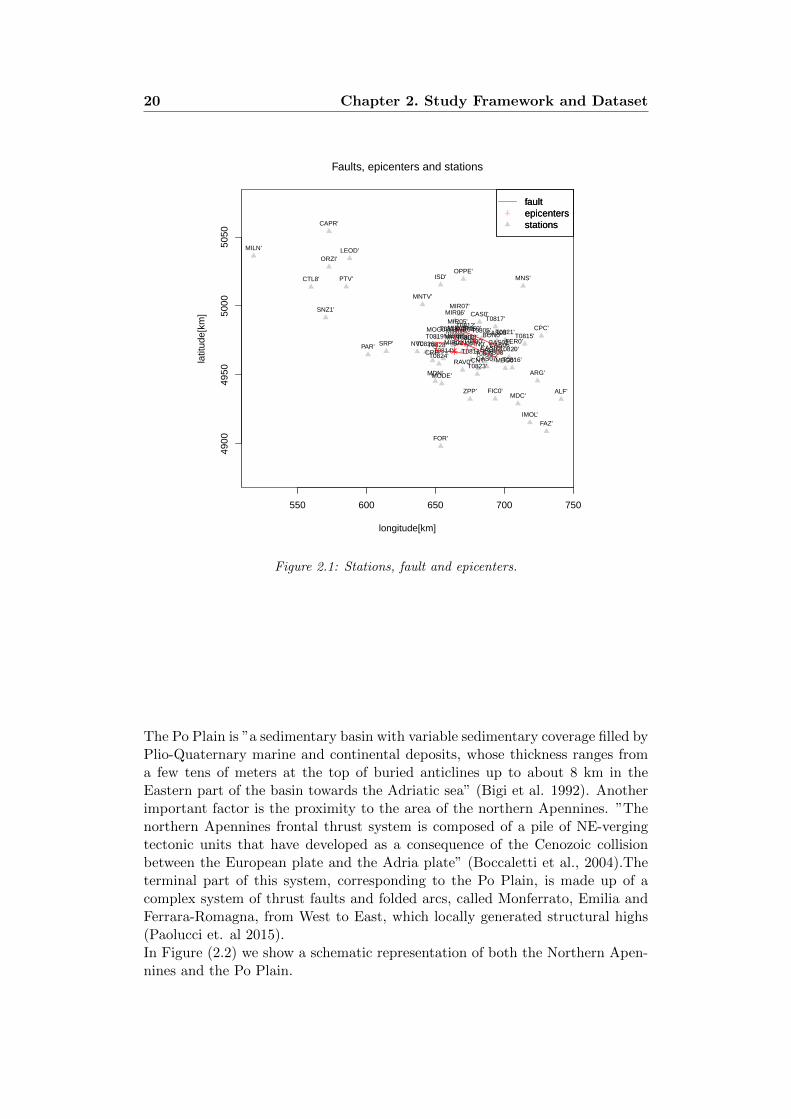
Figure 2.1: Stations, fault and epicenters.
The Po Plain is ”a sedimentary basin with variable sedimentary coverage filled byPlio-Quaternary marine and continental deposits, whose thickness ranges froma few tens of meters at the top of buried anticlines up to about 8 km in theEastern part of the basin towards the Adriatic sea” (Bigi et al. 1992). Anotherimportant factor is the proximity to the area of the northern Apennines. ”Thenorthern Apennines frontal thrust system is composed of a pile of NE-vergingtectonic units that have developed as a consequence of the Cenozoic collisionbetween the European plate and the Adria plate” (Boccaletti et al., 2004).Theterminal part of this system, corresponding to the Po Plain, is made up of acomplex system of thrust faults and folded arcs, called Monferrato, Emilia andFerrara-Romagna, from West to East, which locally generated structural highs(Paolucci et. al 2015).In Figure (2.2) we show a schematic representation of both the Northern Apen-nines and the Po Plain.

2.1. Study Area 21
Figure 2.2: Location of the geological cross-section(red) and the northern Apenninesfrontal thrust(yellow).
As a result of previous researches, some features related to the ground-motioncharacterization of the Po Plain area have come to light:
• The reflection of S waves,in correspondence with the Moho discontinuity,produces the increase of PGA at a distance between 70 km and 200 km(Bragato at al. 2011).
• When the boby waves are trapped in the basin, surface waves are generated(Basin effects). Surface waves mainly determine the seismic signal at periodgreater than 2 seconds (Luzi et al. 2013).
• The presence of a privileged direction of amplification of the surface wavesduring the main event of the 2012 Emilia seismic sequence (Paolucci et al.2015).
Some of the factors, which mainly influenced the near-source ground motionduring the the main event of the 2012 Emilia seismic sequence, are reported inFigure 2.3. with a particular attention to the relation between the buried to-pography and the generation of surface waves created by the irregular geologicalconfiguration(Paolucci et al. 2015).
Figure 2.3: Surface waves generation (Paolucci et al.,2015).
The peculiar structure of the geological cross-section A-A’ passing through theFerrara-Romagna folder arc (Figure 2.3) will be crucial to understand by thephysical point of view the results of our analysis.

22 Chapter 2. Study Framework and Dataset
2.2 Ground Motion Prediction Equation
The Ground Motion Prediction Equation (GMPE) employed to construct thedatasets introduced in Section 2.3 is a model specifically tailored by Lanzano etal.,(2016) for the Northern Italy able to predict the geometric mean of horizontalresponse spectral accelerations in the period range 0.01-4s.
This GMPE by Lanzano et al. (2016) has the functional form:
log10 Y = a+ FM (M) + FD(R,M) + Fsof + FS + Fbas (2.1)
Y is the geometrical mean of the horizontal components of PGA (expressed incm/s2) and SA (in cm/s2) for 24 periods in the range 0.04–4 s with dampingξ=5%.
Members of the model:
• a is the offset.
• FD(R,M) represents the distance function.
• FM (M) is the magnitude scaling.
• FS concerns the site amplification.
• Fsof is the style of faulting.
• Fbas is the basin-effects correction.
R (in km) is the distance, M is the magnitude(if M is missing we adopt Mw orML).ML called Ricther magnitude or local magnitude, is determined at short dis-tances and it is homogeneously determined for small earthquakes up to satura-tion at about ML = 7.0, Mw is the moment magnitude which depends on thesize of the source and the slip along the fault (Douglas 2003).
The distance function has equation:
FD(R,M) = [c1 + c2(M −Mr)] log10
R
Rh(2.2)
where
• c1 and c2 are the attenuation coefficients.
• Mr is a reference magnitude fixed to 5.0.
• R is either the hypocentral distance Rhypo (distance to the hypocenter ofthe earthquake, i.e. the distance to the rupture’s starting point (Douglas
2013)) or the distance computed as√R2JB + h2.
RJB (Joyner–Boore distance) is defined as the distance to the surface pro-jection of the rupture plane of the fault (Douglas 2013).

2.2. Ground Motion Prediction Equation 23
• h is the pseudodepth coefficient.
• Rh is a hinge distance thet takes into account changes in the attenuationrate.
Since attenuation depends on both the geologic domain and distance ranges,equation 2.2 has been modified introducing the index j:
• j=1 if the site is located in PEA(central Po Plain or eastern Alps). andR ≤ Rh
• j=2 if the site is located in PEA and R > Rh.
• j=3 if the site is located in NA (Northen Apenines)and R ≤ Rh.
• j=4 if the site is located in NA and R > Rh.
The new form of equation 2.2 is:
FD(R,M) = [c1j + c2j(M −Mr)] log(R
Rh) j = 1...4 (2.3)
The Rh is set to 70 km. ( Douglas et al. (2003) assumed the same value for thePo Plain area and for central Italy, respectively).To distinguish among the sites located in PEA and NA, a geographic separa-tion has been defined through the linear equation LATref = 0.33LONs + 48.3,in which LONs is the station longitude and LATref is the reference latitude,expressed in decimal degrees.Positive differences between station latitude LATs and LATref identify the PEAsites, and negative differences identify the NA ones.
The magnitude function has the form
FM (M) = b1(M −Mr) + b2(M −Mr)2 (2.4)
The Mr parameter is the reference magnitude, defined in equation (2.2).
The term Fsof in equation (2.1) is needed in order to take into account differentstyles of faulting and is given by
Fsof = fjEj j = NF, TF,UN (2.5)
The coefficients fj in the equation are estimated during the analysis, Ej aredummy variables representing different style of faulting:
• normal (NF)
• thrust (TF)
• unspecified (UN)
24 Chapter 2. Study Framework and Dataset
The term Fs in equation (2.1) represents the site effect and it is defined as follows
Fs = sjSj j = A,B,C (2.6)
In which Sj are dummy variables for the three EC8 site classes A, B, and C.Through regression coefficients sj are estimated.
The term Fs has been introduced to model the bias observed at short periodsin the analysis of ITA10 residuals in the range 30-100 km. This bias is mainlyascribed to C class stations in the Po Plain.
The basin-effect term in equation (2.1) is defined as
Fbas = δbas∆bas (2.7)
in which δbas is the coefficient to be determined during the analysis and ∆bias isa dummy variable equal to 1 if the site is located in the middle of a basin and 0else (Lanzano et al.2016).
2.3 Dataset
In the analysis we use two datasets which have dimension 71 × 25 where thei-th row refers to the i-th station (whose distribution in space can be observed infigures 2.3 and 2.4) and the j-th column to the j-th period in the range 0.01-4s.The first dataset collects the value of the corrective term (δL2L + δP2P +δS2S) while the second one collects the values of σ0,sr computed with a fullynon ergodic approch.
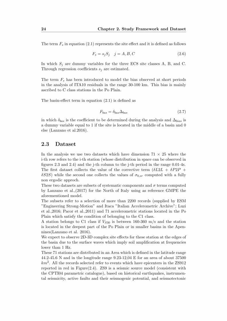
These two datasets are subsets of systematic components and σ terms computedby Lanzano et al.,(2017) for the North of Italy using as reference GMPE theaforementioned model.The subsets refer to a selection of more than 2200 records (supplied by ESM”Engineering Strong-Motion” and Itaca ”Italian Accelerometric Archive”; Luziet al.,2016; Pacor et al.,2011) and 71 accelerometric stations located in the PoPlain which satisfy the condition of belonging to the C1 class.A station belongs to C1 class if VS30 is between 160-360 m/s and the stationis located in the deepest part of the Po Plain or in smaller basins in the Apen-nines(Lanzano et al. 2016).We expect to observe 2D-3D complex site effects for these station at the edges ofthe basin due to the surface waves which imply soil amplification at frequencieslower than 1 Hz.These 71 stations are distributed in an Area which is defined in the latitude range44.2-45.6 N and in the longitude range 9.23-12,04 E for an area of about 37500km2. All the records selected refer to events which have epicenters in the ZS912reported in red in Figure(2.4). ZS9 is a seismic source model (consistent withthe CPTI04 parametric catalogue), based on historical earthquakes, instrumen-tal seismicity, active faults and their seismogenic potential, and seismotectonic
2.3. Dataset 25
evidence from earthquakes since 1998 (Meletti et al. 2008). The model is com-posed of 36 zones (ZS912 is the 12-th zone) where earthquakes with Mw ≥ 5 areexpected and the probability that an earthquake with Mw up to 5 may occursanywhere outside this seismogenic zones is very low (Meletti et al. 2008).
Figure 2.4: Stations and ZS912(red).
The number of available records was crucial because the decomposition of be-tween event residuals and within event residuals in the systematic source termδL2Lr, the path term δP2Ps,r and the site correction δS2Ss can be applied whenempirical datasets are sufficiently populated to estimate each single contribution(Lin et al. 2011).

26 Chapter 2. Study Framework and Dataset

Chapter 3
A univariate approach to thegeostatistical analysis ofintensity measures
3.1 Modelling the Covariance of the Random Field
In this Chapter we describe the univariate methods applied in our analysis. Eachintensity measure will be modelled through a random field Zs, s ∈ D.The random field is a collection of variables having the form
Zs = ms + δs (3.1)
ms is called drift and is the deterministic part of the variable, δs is the randomcomponent.
Definition 2 (Chiles et Delfiner, 1999). Process {Zs, s ∈ D} is said second-orderstationary if the following conditions hold:
• E [Zs] = m for all s in D
• Cov(Zsi , Zsj
)= E
[(Zsi −m)
(Zsj −m
)]= C (h) for all si , sj in D, h =
si − sj.
Function C is called covariogram
Definition 3 (Chiles et Delfiner, 1999). Process {Zs, s ∈ D}is said intrisicallystationary if
• E [Zs] = m for all s in D
• V ar(Zsi − Zsj
)= E
[(Zsi − Zsj
)2]= 2γ (h) for all si , sj in D, h = si −
sj.
The function γ is called semivariogram and the function 2γ variogram.The relation between semivariogram and covariogram is
γ (h) = C (0)− C (h) (3.2)
27

28Chapter 3. A univariate approach to the geostatistical analysis of
intensity measures
Definition 4. An intrinsic stationary process {Zs, s ∈ D} is said isotropic if itsvariogram is isotropic,i.e,
V ar(Zsi − Zsj
)= 2γ (h) h = ||h||
otherwise it is said anisotropic.
When the structure of the covariance is homogenous over all the directions,isotropy is verified. To investigate isotropy, directional variograms are employed.
The variogram is characterized by the nugget, the sill and the range.The sill of the semivariogram is defined as
τ2 + σ2 = limh→∞
γ (h)
where τ2 is the nugget effect and σ2 is said partial sill.The existence of a finite limit indicates that the process is second-order station-ary, featured by a variance C (0) = τ2 + σ2.τ2 is called nugget and it is defined as limh→0 γ (h).The range R of a semivariogram is the value where it reaches the sill:
γ (R) = τ2 + σ2 (3.3)
The semivariogram range quantifies the range of influence of the process: fordistance greater than the range, two elements of the process are uncorrelated.The variogram range can be infinite if the sill does not exist (indication of non-stationarity) or if the sill is reached asymptotically.Given a dataset Zs1 , ..Zsn , under the stationarity assumption, the sample semi-variogram is computed as
γ (h) =1
2 |N (h)|∑
(i,j)∈|N(h)|
[Zsi − Zsj
]2
where N (h) = {(i, j) : ‖si − sj‖ = h} and |N (h)| is its cardinally.After sample estimation, we can fit the sample variogram through a parametricvalid model. In particular in our analysis we’ll use and compare the followingmodels:
• Exponential model:
γ (h) =
{σ2(
1− e−ha
)h > 0
0 h = 0
where a, σ ∈ R. The sill is σ2, the range is infinite, but one can define thepractical range as R = 3a . R satisfies γ(R) ∼ 95%σ2. In this thesis witha slight abuse of notation we will name range the practical range of theexponential model.

3.1. Modelling the Covariance of the Random Field 29
• Spherical model
γ (h) =
0 h = 0
σ2{
32ha −
12
(ha
)3}0 < h < a
σ2 h ≥ a
with a, σ ∈ R. a is the range, σ2 the sill.
The parameters are estimated following the weighted least squares criterion,i.e.,looking for the parameters which minimize
K∑k=1
1
wk
(γ (hk)− γ (hk; θ)
)2(3.4)
where wk, k = 1, ..,K are set to the number of couples N(hk) within each class.
3.1.1 Drift Estimation
When the process is not stationary the mean ms of Model 3.1 is modelled as
ms =
L∑l=0
alfl(s) (3.5)
and we assume residuals stationarity. We can apply drift estimation to performour geostatistical analysis on the residuals.Given Zs1 , ....Zsn , we want to estimate the model parameters a0, ...aL+1 suchthat
Z = Fa+ δ (3.6)
Where F is the design matrix and δ the residuals vector characterized by anunknown covariance structure Σ. If we knew the Σ, we could employ the Gen-eralized Least Square (GLS) estimator to estimate a.This is found by minimizing
(Z − Fa)′Σ−1(Z − Fa) (3.7)
over a ∈ Rp. The GLS estimator aGLS has the form
aGLS = (FΣ−1F )−1FΣ−1Z (3.8)
Through the following iterative algorithm we can jointly estimate γ and a viaGLS and avoid the problem of unknown Σ.Let z = (zs1 , ., zsn) be a realization of the non stationary random field Zs, s ∈ D,D⊆ Rd:
1. Estimate the drift vectorm through the OLS method (mOLS = F (F TF )−1F Tz)and set m = mOLS
2. Compute the residual estimate δ = (δs1 , ., δsn) by difference δ = z − m

30Chapter 3. A univariate approach to the geostatistical analysis of
intensity measures
3. Estimate the semivariogram γ of the residual process {δs, s ∈ D} from δfirst with the empirical estimator and then fitting a valid model.Derive from γ the stimate Σ of Σ
4. Estimate the drift vector m with mGLS , obtained from z usingmGLS = F (F TΣF )−1F TΣ−1z
5. Repeat 2-4 until convergence has been reached.
3.1.2 Geostatistical analysis of the corrective term and σ0,sr
As first step of our geostatistical analysis, we plot the spatial distribution of ourdata. In Figure 3.1 it’s possible to observe how the 71 stations of the datasetare distributed (UTM coordinates).
550 600 650 700 750
4900
4950
5000
5050
Faults, epicenters and stations
longitude[km]
latit
ude[
km]
ALF'
ARG'
BON0'
CAS0'
CNT'
CPC'
CRP'
FAZ'
FER0'
FIC0'
FIN0'
FOR'
ISD'
MBG0'
MDC'
MDN'
MNS'
MOG0'MRN'
NVL'PAR'
PTV'
RAV0'
SAG0'SAN0'
SMS0'
SNZ1'
SRP'
ZPP'
CAPR'
CTL8'
IMOL'
LEOD'MILN'
MNTV'
MODE'
OPPE'
ORZI'
T0800'T0802'
T0803'
T0805'
T0811'
T0812'
T0813'
T0814'
T0815'
T0816'
T0817'
T0818'T0819'
T0820'
T0821'
T0823'
T0824'
T0826'T0828' CAS02'
CAS03'
CAS05'CAS06'
CAS07'CAS08'
MIR01'MIR02'MIR03'MIR04'MIR05'
MIR06'MIR07'
MIR08'
faultepicentersstations
faultepicentersstations
Figure 3.1: Distribution of stations.
The area of study cover a square of side 200 km (a.k.a. bounding box). We fixthe cut-off distance equal to 100 km that is half of the side of the bounding boxfor both the corrective terms δL2L+ δP2P + δS2S and σ0,sr.The cut-off distance is the maximum distance on which the variogram is fitted.In order to understand how the period impacts on the spatial correlation of thecorrective term, we develop our analysis on both the short and the long periodsby considering the PGA and T = 4s.

3.1. Modelling the Covariance of the Random Field 31
3.1.3 Analysis of corrective term
The bubbleplot in Figure 3.2 shows at the same time the position and the valuesof the corrective term for the Peak Ground Acceleration
Figure 3.2: Bubbleplot PGA.
The PGA bubbleplot doesn’t reveal a strong evidence of a spatial trend in thedata. We assume the drift ms constant and unknown.Since there isn’t a strong spatial trend, it is reasonable to assume that the processis intrinsic stationary and to compute both the variogram and the directionalvariograms in order to investigate the isotropic assumption.The directional semivariograms in Figure 3.3 are quite similar in both the rangeand the sill. We thus consider the process Zs as isotropic and we can computethe global sample variogram reported in Figure 3.4.
Figure 3.3: Directional variograms.

32Chapter 3. A univariate approach to the geostatistical analysis of
intensity measures
Figure 3.4: Sample variogram.
The linear behaviour in the origin suggests the application of the spherical modelor the exponential one to fit the sample variogram. We choose the best fittingmodel through Leave-One-Out cross-validation using, as metric, the mean squareprediction error and the mean square prediction error divided by the variance ofprediction (prediction with high variance are weigthed less). Here, prediction ata new location s is made via the Best Linear Unbiased Predictor Zs which willbe used in the following (see Section 3.2):
MSE =1
N
∑(Zs − Zs)2 M2 =
1
N
∑ (Zs − Zs)2
var(Zs)(3.9)
Model MSE M2
Exponential 0.0269 1.0799
Spherical 0.027 1.115
Table 3.1: Model Comparison.
As we can observe in Table 3.1, the exponential model gets better performanceso we decide to use it to fit the sample variogram. We compute the values of theparameter of the model by minimizing weighted least squares.In Table 3.2 we report the values of the parameters and in Figure 3.5 the samplevariogram fitted with the exponential model.
Nugget Psill Range
Exponential 0.0393 32.85
Spherical 0.027 11.15
Table 3.2: Exponential model parameters.

3.1. Modelling the Covariance of the Random Field 33
Figure 3.5: fitted variogram.
We can now compute the covariance for two random variables of the processzsi , zsj thanks to the equation
γ(h) = C(0)− C(h) (3.10)
where C(h) = Cov(zsi , zsj ) with h = si − sj and C(0) = limh→∞γ(h).We repeat the previous geo-statistical analysis for the corrective term at periodT = 4. First we plot the data with bubbleplot.
Figure 3.6: Bubbleplot for corrective term at T = 4s.
As you can observe in Figure 3.6, contrary to what we observed for PGA, theresult shows a positive drift (green bubble) from South-Est toward North-Westin the bottom left of the bubbleplot, a positive drift from North to South inthe center (green bubble) and a negative drift (purple bubble) from East toward

34Chapter 3. A univariate approach to the geostatistical analysis of
intensity measures
West.
Then we want to understand what happens if we don’t care of the drift and wemodel the process {Zs} as intrinsic stationary.A first warning is captured by the directional sample variograms in Figure 3.7,since in different directions the variograms show different behaviours.
Figure 3.7: Directional variograms.
If we try to model a unique sample variogram and to fit it with an exponentialmodel, we obtain a range greater than the cut-off distance that is an indicationthat, at the scale of observation, the process cannot be considered as stationary.
Fitted Variogram With Exponential Model T=4s log10[cm/s^2]
distance[km]
sem
ivar
ianc
e
0.02
0.04
0.06
0.08
20 40 60 80
●
●
●
●
●
●
●
●
●
●
●
●
●
●
●
Figure 3.8: Sample variogram fitted.
We can’t assume the intrinsic stationary assumption so it means that ms is afunction of the s coordinates. The idea is that the random field can be seen as
3.1. Modelling the Covariance of the Random Field 35
the sum of a deterministic surface ms and an aleatory second-order stationarycomponent δs. If we can learn the surface representing the drift, then we canmodel the covariance of the residuals δs through the variogram. We try to modelthe drift with polynomial surfaces of degree 1 to 4:
1. ms = β0 + β1x+ β2y
2. ms = β0 + β1x+ β2y + β3x2 + β4y
2 + β5xy
3. ms = β0 + β1x+ β2y+ β3x2 + β4y
2 + β5xy+ β6x2y+ β7yx
2 + β8x3 + β9y
3
4. ms = β0 +β1x+β2y+β3x2 +β4y
2 +β5xy+β6x2y+β7yx
2 +β8x3 +β9y
3 +β10x
4 + β11y4 + β12xy
3 + β13x3y
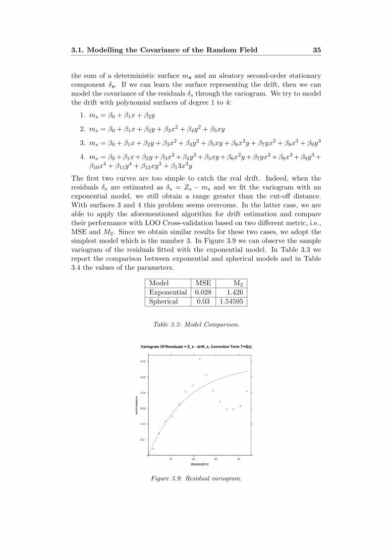
The first two curves are too simple to catch the real drift. Indeed, when theresiduals δs are estimated as δs = Zs − ms and we fit the variogram with anexponential model, we still obtain a range greater than the cut-off distance.With surfaces 3 and 4 this problem seems overcome. In the latter case, we areable to apply the aforementioned algorithm for drift estimation and comparetheir performance with LOO Cross-validation based on two different metric, i.e.,MSE and M2. Since we obtain similar results for these two cases, we adopt thesimplest model which is the number 3. In Figure 3.9 we can observe the samplevariogram of the residuals fitted with the exponential model. In Table 3.3 wereport the comparison between exponential and spherical models and in Table3.4 the values of the parameters.
Model MSE M2
Exponential 0.028 1.426
Spherical 0.03 1.54595
Table 3.3: Model Comparison.
Figure 3.9: Residual variogram.

36Chapter 3. A univariate approach to the geostatistical analysis of
intensity measures
Nugget Psill Range
0.00 0.055 98.55
Table 3.4: Exponential model parameters.
The correlation coefficient ρ(h) in case of exponential model is
ρ(h) = exp(−h/a) a =range
3(3.11)
We can compare the shapes of the correlation coefficients, as function of h, forboth PGA and T = 4s.
Figure 3.10: Comparison of correlation coefficients.
The random field of the PGA looses the correlation faster than T = 4s. Indeed,the range of PGA is lower than the one related to the period T = 4s.The correlation of spectral intensity measures is period-dependent because shortperiod waves tend to be more affected by the heterogeneities of the propagationpath, thus resulting correlated at a shorter scale than long period ground motions(Zerva et Zervas, 2002; Bradley, 2014).
3.1.4 Analysis of σ0,sr
We repeat the statistical analysis, already performed for the corrective termdataset, also for the variance term σ0,sr working again with PGA and T = 4s.In Figure 3.11 and Figure 3.12 the Bubbleplot doesn’t show an evident non-costant drift and the directional variograms are quite similar in all directions sowe can assume that the random field is second-order stationary and isotropic.

3.1. Modelling the Covariance of the Random Field 37
Sigma PGA log10[cm/s^2]
●●
●
●
●
●
●
●
●
●
●
●
●
●
●
●
●
●●●●
●
●●●
●●
●
●
●
●
●
●●
●
●
●●
●●●
●
●
●●
●●
●
●●●
●●
●●
●● ●●
●●●●
●●●●●●●
●
●●●●●
0.120.1940.230.2650.348
Figure 3.11: Bubbleplot and directional variogram PGA.
Sigma T=4s log10[cm/s^2]
●●
●
●
●
●
●
●
●
●
●
●
●
●
●
●
●
● ●●●
●
●●●
●●
●
●
●
●
●
●●
●
●
●●
●●●
●
●
●●
●●
●
●●●
●●
●●
●● ●●
●●●●
●●●●●●●
●
●●●●●
0.1320.190.2320.2670.388
Figure 3.12: Bubbleplot and directional variogram T = 4s.
The exponential model, again, gets a better MSE with LOO Cross Validationthan the spherical one, as reported in Table 3.5 and Table 3.6.
Model MSE M2
Exponential 0.0002739 1.2
Spherical 0.002762 1.23
Table 3.5: Model Comparison PGA.

38Chapter 3. A univariate approach to the geostatistical analysis of
intensity measures
Model MSE M2
Exponential 0.000234 1.008
Spherical 0.002531 1.14
Table 3.6: Model Comparison SA(T = 4s).
So the sample variogram is fitted through an exponential model whose parame-ters are reported in Tables 3.7 and Table 3.8.
Nugget Psill Range
0.0009 0.0021 37.2
Table 3.7: Exponential model parameters PGA.
Nugget Psill Range
0.00 0.0029 12
Table 3.8: Exponential model parameters SA(T = 4s).
Figure 3.13: Variogram of PGA and on the left and variogram of SA(T = 4) on theright fitted with the exponential model.
At the end, we compute the ρ(h) of the random field PGA and SA(T = 4)in order to compare how the correlation decreases as function of the period.Contrary to what we observed for the corrective term, the covariance functionof PGA is now generally above the one corresponding to SA(T = 4) (i.e., therange for the PGA is higher than that of SA(T = 4)); however, the two curvesare closer than ones in the case of corrective term.

3.2. Kriging 39
Figure 3.14: Comparison of correlation coefficients of PGA and SA(T = 4s).
3.2 Kriging
3.2.1 Introduction
After modelling the covariance of the random field associated to different pe-riods of the corrective term and of σ0,sr, we want to predict their values in anew location. The kriging predictor linearly combines the data in the availablelocations and predicts the values of the random field in an arbitrary location asZs0 =
∑ni=1 λiZsi = λTZ , where the weights are found according to the field
covariance structure (computed in Section 3.1). We can distinguish among 3types of kriging:
1. Simple: Simple kriging is employed for random fields with known drift.The weights are found by solving:
Σλ = σ0
where
Σ =[Cov
(Zsi , Zsj
)], σ0 = [Cov (Zsi , Zs0)]
2. Ordinary: Ordinary kriging is employed for random fields with constantunknown mean. The optimal weights are solution of the system(
Σ 11 0
)(λβ
)=
(σ01
)
where β are Lagrange multiplier.

40Chapter 3. A univariate approach to the geostatistical analysis of
intensity measures
3. Universal: Universal kriging is employed for random fields with variabledrift. The Universal kriging predictor is obtained from
(Σ FF T 0
)(λβ
)=
(σ0
f0
)
where f0 = [fl (s0)],F = [fl (si)] is the design matrix, and β = (β0, .., βl)is the vector of Lagrange multipliers accounting for the constrains:
n∑i=1
λifl (si) = fl (s0) , l = 1, ..., L.
For more details about kriging see Chiles et Delfiner (1999).
3.2.2 Kriging for the corrective terms
The random field of the corrective term of PGA has been modelled in the pre-vious section considering a constant and unknown drift. We can employ theordinary kriging predictor to estimate the random field on a grid of 70000 pointscovering the Area of study. In Figure 3.15 we report the prediction and the re-lated variance and in Figure 3.16 we zoom on the zone of the faults in which therectangle on the left represent the projection of the fault planes on the surfaceof the second main events of 2012 Emilia seismic sequence and the one on theright of the first main event.
550 600 650 700
4900
4950
5000
5050
Variance Of Prediction Of Corrective Term−PGA log10[cm/s^2]
Xgrid
Ygr
id
0.01
0.02
0.03
0.04
FaultsStationsEpicenters
Figure 3.15: Ordinary kriging prediction and variance for PGA.
3.2. Kriging 41
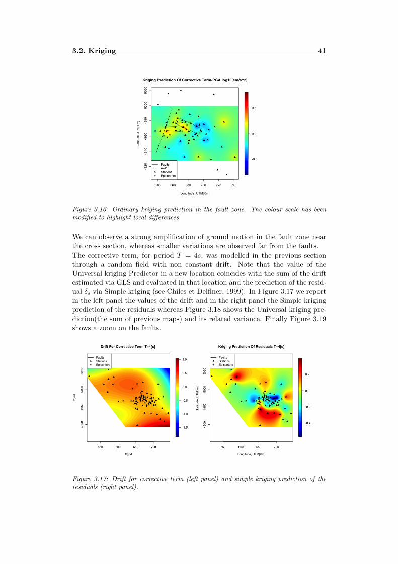
Figure 3.16: Ordinary kriging prediction in the fault zone. The colour scale has beenmodified to highlight local differences.
We can observe a strong amplification of ground motion in the fault zone nearthe cross section, whereas smaller variations are observed far from the faults.The corrective term, for period T = 4s, was modelled in the previous sectionthrough a random field with non constant drift. Note that the value of theUniversal kriging Predictor in a new location coincides with the sum of the driftestimated via GLS and evaluated in that location and the prediction of the resid-ual δs via Simple kriging (see Chiles et Delfiner, 1999). In Figure 3.17 we reportin the left panel the values of the drift and in the right panel the Simple krigingprediction of the residuals whereas Figure 3.18 shows the Universal kriging pre-diction(the sum of previous maps) and its related variance. Finally Figure 3.19shows a zoom on the faults.
Figure 3.17: Drift for corrective term (left panel) and simple kriging prediction of theresiduals (right panel).

42Chapter 3. A univariate approach to the geostatistical analysis of
intensity measures
Figure 3.18: Universal kriging prediction and variance of corrective term at T = 4s.
Figure 3.19: Universal kriging prediction (zoom). The colour scale has been modified tohighlight local differences.
As already observed for PGA, in the fault zone we have a strong amplificationof the motion. This ground motion amplification could be linked to the complexgeological structure of the cross-section A-A’. Surface waves, which are gener-ated in direction A-A’ where the thickness of the Quaternario sediment coverdecreases, mainly determine the seismic signal at period greater than 2 seconds.This element is too complex to be captured by the ground motion predictionequations. Additionally we can observe a strong amplification in the South ofthe Area which corresponds to the Appenninic area. This amplification is notobserved in PGA.

3.2. Kriging 43
3.2.3 Kriging for σ0,sr
The random field of σ0,sr has been modelled as an isotropic process with constantand unknown drift for both PGA and T = 4s so we can use ordinary krigingto predict the values on the grid. We report the maps for the prediction andvariance in Figure 3.20 and 3.21, and a zoom on the faults in Figures 3.22.
Figure 3.20: Ordinary kriging prediction and variance for the PGA.
Figure 3.21: Ordinary kriging prediction and variance of SA(T = 4s).

44Chapter 3. A univariate approach to the geostatistical analysis of
intensity measures
640 660 680 700 720 740
4920
4940
4960
4980
5000
5020
kriging Prediction of Sigma PGA log10[cm/s^2]
Longitude, UTM[Km]
Latit
ude,
UT
M[k
m]
0.0
0.1
0.2
0.3
0.4
FaultsA−A'Stations Epicenters
Figure 3.22: Ordinary kriging prediction of PGA and SA(T = 4s), zoom on the faults.The colour scale has been modified to highlight local differences.
Comparing the PGA and T = 4s kriging predictions for σ0,sr we observe thaton the whole grid PGA has lower values but on the fault zone PGA and T = 4sare very similar. We have a greater amplification from East to West below thefaults zone.
3.3 Conditional Simulation
3.3.1 Introduction
The kriging prediction represents the average scenario. We would like to takeinto account the variability of the range of scenarios compatible with the data tounderstand what the best and worst case scenarios could be in a certain location.In order to consider the variance related to the prediction, we could simply addto the prediction the realization of a Gaussian noise centered in zero and withvariance the kriging variance. However, this would neglect the spatial depen-dence among close locations. A better way to include the variance is representedby the Conditional Simulation.Here we summarize the main concepts of the conditional simulation in the Gaus-sian case, by following (Chiles et Delfiner, 1999), with a particular reference toSequential Gaussian Simulation.Let Z = (Z1, Z2, ..., ZM , .., ZN )′ be a vector collecting the random variables Ziof the random field and suppose that we know the realization of the subvector(Z1 = z1, Z2 = z2, ..ZM = zm).Then the conditional distribution of Z given Zi = zi, i = 1, ...,M , can be factor-ized in the form
Pr {zM+1 ≤ ZM+1 < zM+1 + dzM+1, ...., zn ≤ ZN < zN + dzN |z1, ..zM} =

3.3. Conditional Simulation 45
Pr {zM+1 ≤ ZM+1 < zM+1 + dzM+1|z1, ..zM}×
Pr {zM+2 ≤ ZM+2 < zM+2 + dzM+2|z1, ..zM , zM+1} × ...×
Pr {zn ≤ ZN < zN + dzn|z1, ..zM , zM+1, ..ZN−1}
Therefore, we can simulate the vector Z sequentially by randomly selecting Zifrom the conditional distribution and including the outcome zi in the condition-ing dataset for the next step.Once we have fixed a grid, the sequential simulation algorithm, following astochastic path through the grid, repeats the following step (Bivand et al., 2013):
1. Computing the parameters of the conditional distribution based on boththe original data and the values previously sampled
2. Sampling a new value
3. Adding the value to the dataset
4. Reaching a new location of the grid following the random path
At every new simulation (i.e. at every step of the Algorithm) the computationaleffort of point 1 increases and it takes more time to compute a new simulation. Toavoid this problem, it is possible to set a maximum number of neighbourhoods (inour case 40) with respect to which computing the conditional distribution(Bivandet al. 2013). Here below we report the computation of parameters of point 1 incase of Gaussian random field recalling the definition of the Multivariate NormalDistribution and its conditional law(Chiles et Delfiner, 1999).
Definition 5 (Johnson et Wicherin). A p-dimensional normal density for therandom vector Z = [Z1, ...Zp]
′ has the form:
f(z) =1
2πp2 |Σ|
12
e(z−µ)′Σ−1(z−µ)/2
where −∞ < zi < ∞, i = 1, 2, .., p, µ is a p×1 vector and Σ is a p×p positivedefinite matrix.We shall denote this p-dimensional normal density by Z ∼ Np(µ, Σ)
Property 1. Let Z=
[Z1
Z2
]be distributed as N(µ,Σ)with :
µ =
[µ1
µ2
], Σ =
[Σ11 Σ12
Σ21 Σ22
], |Σ22| > 0
Then the conditional distribution of Z1 , given that Z2 = z2, is normal and hasmean
µ1 + Σ12Σ22−1 (z2 − µ2)
and covariance

46Chapter 3. A univariate approach to the geostatistical analysis of
intensity measures
Σ11 −Σ12Σ22−1Σ21
The Gaussian random fields assumption commonly adopted in geostatistics hasbeen introduced in the geostatistical applications by Alabert and Massonat(1990)(Chiles et Delfiner, 1999).In the seismology framework, other studies focused on the spatial correlationwithin event residuals adopted the same assumption. The assumption has beenintroduced in the applied seismology framework by (Park et al.,(2007)); Verroset al (2017) applied successive conditional simulation in order to estimate thewithin event residual, Baker et al. (2007) simulated the global residuals for lossestimation and Bradley et al. (2014) applied the conditional simulation basedon the Gaussian distribution of within event residuals to develop a PGA mapfor the 2010-2011 Cantebury earthquakes.In the next section we show the results of our conditional simulation applied toboth the corrective term and σ0,sr.
3.3.2 Sequential simulation for corrective term
Figure 3.23 represent the comparison between a simulated scenario and the krig-ing for the corrective term of PGA in the same scale.
Figure 3.23: The kriging prediction and the conditional simulation for PGA.
We observe that, in the conditional simulation, maps are more rough than theones of the kriging prediction; these scenarios differ from each other but we canalso observe a common trends in the fault zone. We can consider a simulationand kriging prediction focused on the fault zone as reported in Figure 3.24.

3.3. Conditional Simulation 47
Figure 3.24: The kriging prediction and the conditional simulation, faults zone for PGA.The colour scale has been modified to highlight local differences.
We observe a strong amplification of the ground motion near the faults and thecross section A-A’ and that the simulated amplifications reach higher values andcover a largest area in the fault zone than the kriging prediction. The krigingprediction represents the average scenario, this imply that in zone of greateramplification than kriging, there will be simulations with a smaller amplificationand, as consequence, the worst case scenario (strong amplification) and the bestcase scenario (deamplification) are very different near the fault zone. As forPGA, we report the sequential simulation for period T = 4s. In Figure 3.25 wecan observe the conditional simulations and the universal kriging prediction inthe same scale.
Figure 3.25: Comparison between the average scenario and the simulation T=4s.

48Chapter 3. A univariate approach to the geostatistical analysis of
intensity measures
Figure 3.26: The kriging prediction and the conditional simulations for SA(T=4s), faultszone. The colour scale has been modified to highlight local differences.
The simulations assign to the three stations belonging to Appenninies, in thenorth of the map, higher values than the universal kriking prediction. StrongerAmplification with respect to the average scenario could be consequence of com-plex 2D and 3D site effects due to the presence of surface waves generated atthe basin edges, with remarkable soil amplification at frequencies smaller than1HZ(Lanzano et al.,2016).
3.3.3 Sequential simulation for σ0,sr
The variable σ0,sr represents the aleatory uncertanty of the GMPE prediction.If the corrective terms and the GMPE captured all the systematic effects thatinfluence the ground motion intensities in a specific location, then σ0,sr in thatlocation would be very low. This entails that for the Area, in which we havegreater values of σ0,sr, we are not modelling all the complex sources and thepropagation effects.Let’s consider first the PGA. In Figure 3.27 in the left panel we can observe theordinary kriging prediction of σ0,sr and in the right we add the uncertainty inthe kriging prediction through the conditional simulation:

3.3. Conditional Simulation 49
550 600 650 700
4900
4950
5000
5050
Conditional Simulation−Sigma PGA log10[cm/s^2]
Xgrid
Ygr
id
0.0
0.1
0.2
0.3
0.4
FaultsStations Epicenters
Figure 3.27: The kriging prediction and the conditional simulation.
Under the two faults, we notice a lighter area from East to West in which σ takesthe greatest values. This trend indicates that in this area the model doesn’tperform as well as in the other ones.With a focus on the fault zone, it is easier to observe the trend.
640 660 680 700 720 740
4920
4940
4960
4980
5000
5020
Conditional Simulation−Sigma PGA log10[cm/s^2]
Longitude, UTM[Km]
Latit
ude,
UT
M[k
m]
0.0
0.1
0.2
0.3
0.4
FaultsA−A'StationsEpicenters
Figure 3.28: The kriging prediction and the conditional simulation, faults zone. Thecolour scale has been modified to highlight local differences.
In Figure 3.28 the aforementioned spatial trend is clearly visible both in thekriging prediction and in the simulation. The simulation higlights that σ0,sr
could be even bigger in the zone around the faults and near the cross sectionA-A’. We report the same plot for T = 4 s.

50Chapter 3. A univariate approach to the geostatistical analysis of
intensity measures
550 600 650 700
4900
4950
5000
5050
Conditional Simulation−Sigma T=4[s] log10[cm/s^2]
Xgrid
Ygr
id
0.0
0.1
0.2
0.3
0.4
FaultsStationsEpicenters
Figure 3.29: The kriging prediction and the conditional simulation.
The first result we observe is that the distribution is much more scattered andthere isn’t a clear zone where sigma has greater values. This observation isconfirmed by the zoom on the fault area.
640 660 680 700 720 740
4920
4940
4960
4980
5000
5020
Conditional Simulation−Sigma T=4[s] log10[cm/s^2]
Longitude, UTM[Km]
Latit
ude,
UT
M[k
m]
0.0
0.1
0.2
0.3
0.4
FaultsA−A'StationsEpicenters
Figure 3.30: The kriging prediction and the conditional simulation, faults zone. Thecolour scale has been modified to highlight local differences.

3.3. Conditional Simulation 51
3.3.4 Comparison of different periods in the faults zone
Figure 3.31: Comparison of conditional simulation, corrective term, PGA in left paneland Sigma SA(T=4s) in the right panel.
640 660 680 700 720 740
4920
4940
4960
4980
5000
5020
Conditional Simulation−Sigma PGA log10[cm/s^2]
Longitude, UTM[Km]
Latit
ude,
UT
M[k
m]
0.0
0.1
0.2
0.3
0.4
FaultsA−A'StationsEpicenters
640 660 680 700 720 740
4920
4940
4960
4980
5000
5020
Conditional Simulation−Sigma T=4[s] log10[cm/s^2]
Longitude, UTM[Km]
Latit
ude,
UT
M[k
m]
0.0
0.1
0.2
0.3
0.4
FaultsA−A'StationsEpicenters
Figure 3.32: Comparison of conditional simulation, σ0,sr PGA in left panel and σ0,srSA(T=4s) in the right panel.
The comparison between the corrective term at PGA and T = 4s highlights thatfor both periods we can observe the amplification of the ground motion in the

52Chapter 3. A univariate approach to the geostatistical analysis of
intensity measures
direction A-A’ and that in the Appenninic area the amplification is much morestronger for T = 4s than for PGA.

Chapter 4
Functional geostatistics for thejoint analysis of intensitymeasures over a range ofperiods
4.1 State Of The Art
In the previous section we have considered four scalar random fields, namely thecorrective term for PGA and SA(T = 4), and σ0,sr for PGA and SA(T = 4).These models, unfortunately, don’t take into account the correlation among SAat different periods as they only describes the correlation of SA at the sameperiods in different stations through different kriging techniques.We are not taking advantage of all the available information. We could think toemploy a multivariate approach and consider a vector random field Zs, whichare vectors collecting all the twenty five periods of our dataset in different loca-tions s.This multivariate framework has been already applied by Loth (Loth and Baker,2012) for the whithin event residuals, to model the spatial correlation of thespectral acceleration at six natural periods.In our case, the number of periods is too high to employ the cross-covariograms.Indeed, fitting the variogram and cross-variogram models jointly for all periodswould require to each period to have the same range and this is not feasible whenone deal with vectors of twenty five components. Even if the fitting is possible,we would have to deal with the sequential simulation of 25 periods which needsa huge computational effort.For this reason, we adopt a functional geostatistics approach instead of the mul-tivariate framework. Functional geostatistics is a subfield of Object OrientedSpatial Statistics, a collection of techniques, algorithms and methods focusedon the analysis of high dimensional and complex data. Typically, spatial dis-tributions of curves and surfaces are the objects of the analysis (Menafoglio etal. 2017). The use of this approach to the problem we are considering would
53

54Chapter 4. Functional geostatistics for the joint analysis of intensity
measures over a range of periods
allow to smooth the data, to manage their intrinsic noise and to compute, in aprediction or simulation setting, the value of SA at any arbitrary period in therange PGA and T = 4s even if that period is not present in the dataset. Indeed,the model allows to recreate the entire shape of the corrective term and σ at allperiods between PGA and T = 4s.In the context of simulation of stochastic processes of functional data spatiallydistributed, we here follow the approach of Menafoglio et al. (2016), who pro-pose to employ functional principal component analysis (FPCA) first, and thenkriging and stochastic simulation of the FPC scores. An application to real dataof the decomposition of the curves into a functional basis in order to move froma problem of kriging in infinite dimensional space to cokriging on basis coeffi-cients is also proposed by Nerini et. al, (2009). In the next section we proposean application of these methods to seismology. This is a turning point for thedevelopment of seismic methods not based on a single period but on the jointconsideration of all periods.For more details about functional geostatistics see Delicado et. al,(2009).
4.2 Functional Data Analysis
4.2.1 Introduction
Given a set of discrete measured values y1, ., yn representing the images (or theimages plus a noise) of a certain function x(t) evaluated in t1, ., tn the first stepof an analysis in the framework of Functional Data Analysis is to reconstruct thecurve x(t). This operation can be done through interpolation or by smoothing.In the first case we want to find a function able to pass through all yi, in thesecond one we consider yi as noisy data so that we want a function which passesonly close to the points in order to avoid to fit the error.
4.2.2 Representing functions by basis functions
A basis for a functional space is a collection of functions φk k = 1, ...,K such thateach function of that space can be represented as the weighted linear combinationof those functions φk
x(t) =
K∑k=1
ckφk(t) (4.1)
or in vector notation:
x(t) = c′φ (4.2)
where φ is the column vector collecting the functions φk(t) in the basis.
Through K we can control the degree of smoothing the data yj . We aim to usethe smallest number K of functions φk able to reflect the features of the data.

4.2. Functional Data Analysis 55
4.2.3 Spline functions
Here we want to describe a spline function of order m on the interval [a, b] withknots (or breakpoints) τl ,l = 1, ..., L+ 1.In order to construct a spline function on the interval [a, b], the first step isto separate the interval [a, b] in L subintervals in some arbitrary points τl ,l =1, ..., L + 1 called knots or breakpoints. τ1=a and τL+1 = b are the externalbreakpoints. On each of these subintervals the spline function is a polynomialof order m where the order of a polynomial, by definition, is the number of hiscoefficients (e.g y = ax+ b has order 2) while the degree is the highest power ofx (e.g y = ax+ b has order 1).Adjacent polynomials join up smoothly at the breakpoint which separates them.The polynomials are constrained to be equal at their junction so the spline is acontinuous function on [a, b]. In addition, all the derivates up to the (m − 2)thmust also match up at these junctions.The degree of freedom of the spline is define as the sum of the order(m) and thenumber of interior points (L− 1) and it represents the flexibility in the fit of thespline.
4.2.4 The B-spline basis for spline functions
A basis for the space of splines of order m on interval [a, b] with knots τ is acollection of functions φk(t) which satisfies:
• each φk(t) is a spline of order m on [a, b] and knot τ .
• every linear combination of φk(t) is a spline function.
• every spline function of order m, knots τ on [a,b] can be expressed as alinear combination of these φk(t)
.
The basis can be created in several ways and the most popular one was introducedby De Boor (2001). The last important property to consider is that the space ofSpline of order k on [a, b] with knots τ is contained in the space of the Splineson the same interval, with the same knots and order m+ 1.
4.2.5 Smoothing Functional Data By Least Squares
We consider our data yi as the sum of a deterministc model x(t) and a noise ε:
yj = x(tj) + εj (4.3)
and we aim to learn the function x(t). First we can see the function as the linearcombination of a vector of weights and the functions of a basis
x(t) =
K∑k
ckφk(t) = c′φ (4.4)

56Chapter 4. Functional geostatistics for the joint analysis of intensity
measures over a range of periods
where the vector c of length K contains the coefficients ck. Now we need toestimate the coefficients able to minimizing the sum of square errors which isdefined as
SMSSE(y|c) = (y −Φc)′(y −Φc) (4.5)
where Φ is the n (number of knots) × K (number of functions in the basis)matrix containing the values φk(tj). By setting the derivative of SSE(y|c) withrespect to c at zero we obtain:
2ΦΦ′c− 2Φ′y = 0 (4.6)
Finally solving the equation with respect to c, we can find c that minimizesthe least square criterion and the values of the target variable estimated by themodel y
c = (Φ′Φ)−1Φ′y (4.7)
y = Φc = Φ(Φ′Φ)−1Φ′y (4.8)
4.2.6 Smooting functional data with a roughness penality
The spline smoothing method, previously described, is able to find the functionthat minimizes the sum of square erros.∑
[yj − x(tj)]2 (4.9)
If the function has sufficient degrees of freedom,by minimizing SSE, it tendsto interpolate all the points. However, on the one hand we want to ensure agood fit of the data on the other hand we don’t want to fit the noise. In orderto avoid interpolation, we penalize the functions x(t) that are too much locallyvariable and manifest a rapid local variation. First we have to define the functionroughness.
4.2.7 Roughness
The curvature of a function x(t) in t is defined as the square of the secondderivative [D2x(t)]2. Note that straight lines, as we expected, have zero curvatureaccordingly with this definition. The roughness is defined as the integral over thedomain of the curvature(or the square of the L2 norm of the second derivative):
PEN2(x) =
∫[D2x(s)]2ds (4.10)
Functions x(t) which manifests rapid local variation in the first derivative willhave high PEN2(x) value. Instead of minimize SSE, to avoid overfitting, we’lllook for function x(t) able to minimize PENSSEλ define as
PENSSEλ(x|y) := SSE + λPEN2(x) (4.11)

4.3. Application to data 57
In this framework a famous theorem (De Boor, 2002) ensures that the functionthat minimize these quantity is a cubic spline with knots in tj , j = 1, ..., n, where(t1, y1)...(tn, yn) are the observed data. Then, as basis, we could employ a B-spline basis of order four and same knots. The method is often called cubicspline smoothing. As we did for SSE, we compute the coefficients c of the modeland the predicted values. First we expess PEN2(x) in vector notation as
PEN2(x) = c′Rc (4.12)
where
R =
∫DmΦ(s)DmΦ(s)′ds (4.13)
and φ(t) is the column vector collecting the basis functions evaluated in tPENSSEλ can be rewritten as:
PENSSEm(y|c) = (y − Φc)′(y − Φc) + λc′Rc (4.14)
To find the value c that minimizes the quantity compute the derivative and setequal to 0
− 2Φ′y + ΦΦc+ λRc = 0 (4.15)
By solving the equation with respect to c we find c:
c = (Φ′Φ + λR)−1Φy (4.16)
4.3 Application to data
First we want to study the corrective term. To each of the 71 stations we havelinked a vector of 25 components which represents SA at 25 different periods,from PGA to T = 4s.In Figure 4.1 we plot simultaneously all the 71 station. Each vector is reportedas a collection of segments obtained by linking the single values observed in thatspecific station.
Figure 4.1: The original corrective terms at different periods, for different stations.
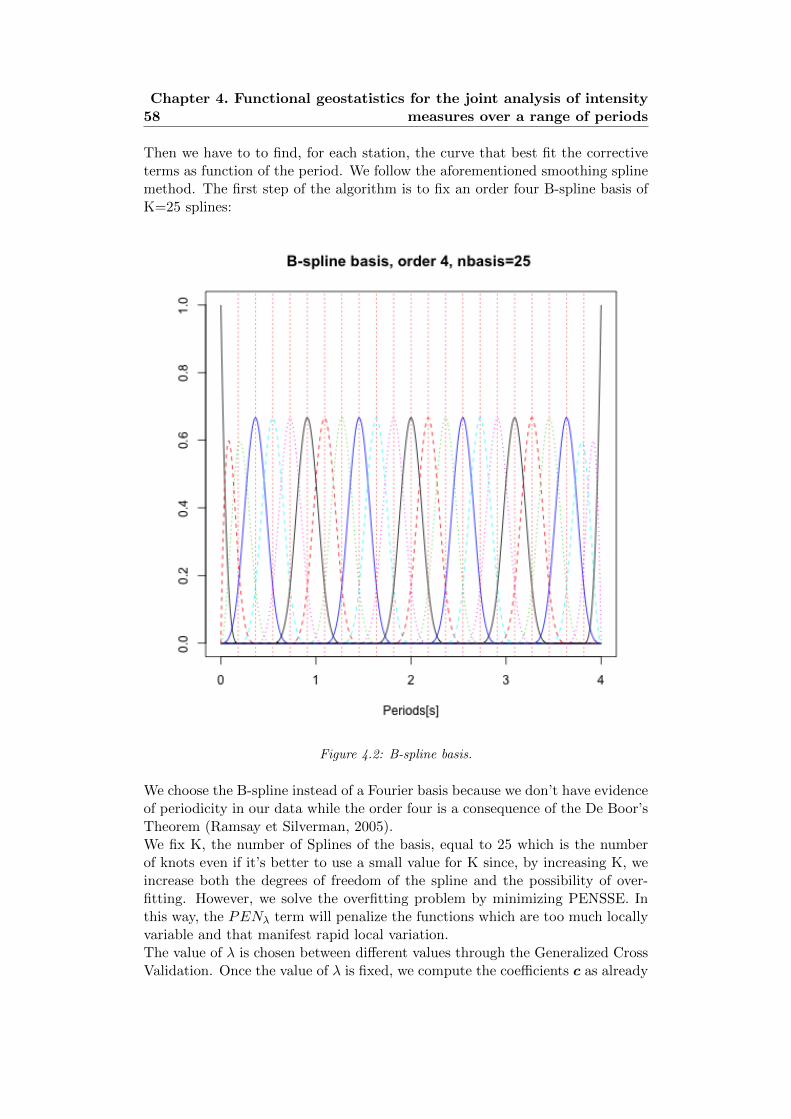
58Chapter 4. Functional geostatistics for the joint analysis of intensity
measures over a range of periods
Then we have to to find, for each station, the curve that best fit the correctiveterms as function of the period. We follow the aforementioned smoothing splinemethod. The first step of the algorithm is to fix an order four B-spline basis ofK=25 splines:
Figure 4.2: B-spline basis.
We choose the B-spline instead of a Fourier basis because we don’t have evidenceof periodicity in our data while the order four is a consequence of the De Boor’sTheorem (Ramsay et Silverman, 2005).We fix K, the number of Splines of the basis, equal to 25 which is the numberof knots even if it’s better to use a small value for K since, by increasing K, weincrease both the degrees of freedom of the spline and the possibility of over-fitting. However, we solve the overfitting problem by minimizing PENSSE. Inthis way, the PENλ term will penalize the functions which are too much locallyvariable and that manifest rapid local variation.The value of λ is chosen between different values through the Generalized CrossValidation. Once the value of λ is fixed, we compute the coefficients c as already

4.3. Application to data 59
explained in the last section.We report the smoothing splines and the original data for some stations locatedin the Appenninic Area and in the faults zone(Figures 4.3).
660 680 700 720 740
4910
4920
4930
4940
4950
4960
4970
4980
Faults, epicenters and stations
longitude[km]
latit
ude[
km]
BON0'
FAZ'
FIC0'MDC'
SAG0'
SAN0'
SMS0'
IMOL'
faultepicentersstations
faultepicentersstations
Figure 4.3: Stations located in the Appenninic Area and in the faults zone.
0 1 2 3 4
−0.
4−
0.3
−0.
2−
0.1
0.0
Spline Smoothing Station 'IT.SAG0'
periods[s]
Cor
rect
ive
Term
log1
0[cm
/s^2
]
●
●
●
●
●
●
●
●
●
●
●
●
●
●
●
●
●
●
●●
●
●
●
●●
Spline SmoothingOriginal Data●
0 1 2 3 4
−0.
15−
0.10
−0.
050.
000.
05
Spline Smoothing Station 'IT.SMS0'
periods[s]
Cor
rect
ive
Term
log1
0[cm
/s^2
]
●
●
●
●
●●
●
●
●
●
●
●
●
●
●
●
●
●
●
●
●●
●
●
●
Spline SmoothingOriginal Data●
Figure 4.4: Smoothing spline for Stations SAG0 and SMS0.
0 1 2 3 4
−0.
50−
0.45
−0.
40−
0.35
−0.
30
Spline Smoothing Station 'IT.BON0'
periods[s]
Cor
rect
ive
Term
log1
0[cm
/s^2
]
●
●
●
●
●
●
●
●
●
●●
●
●
●
●
●
●
●
●●
●
●
●
●
●
Spline SmoothingOriginal Data●
0 1 2 3 4
−0.
20−
0.15
−0.
10−
0.05
0.00
Spline Smoothing Station 'IT.SAN0'
periods[s]
Cor
rect
ive
Term
log1
0[cm
/s^2
]
●
●
●
●
●
●
●
●
●
●
●
●
●
● ●● ● ●
●
●
●
●
●
●
●
Spline SmoothingOriginal Data●
Figure 4.5: Smoothing spline for stations BON0 and SAN0.

60Chapter 4. Functional geostatistics for the joint analysis of intensity
measures over a range of periods
0 1 2 3 4
0.0
0.2
0.4
0.6
Spline Smoothing Station 'IT.FIC0'
periods[s]
Cor
rect
ive
Term
log1
0[cm
/s^2
]
●
●
●
●
●
●
●
●
●
●
●
●
●
●
●
●
●
●●
●
●●
●
●
●
Spline SmoothingOriginal Data●
0 1 2 3 4
−0.
20.
00.
20.
4
Spline Smoothing Station 'FAZ'
periods[s]
Cor
rect
ive
Term
log1
0[cm
/s^2
]
●
●
●
●
●
●
●
●
●
●
● ●
●
●●
●
●●
●
●
●
●
●
●
●
Spline SmoothingOriginal Data●
Figure 4.6: Smoothing spline for stations FICO,FAZ.
0 1 2 3 4
−0.
3−
0.2
−0.
10.
00.
10.
20.
3
Spline Smoothing Station 'IT.IMOL'
periods[s]
Cor
rect
ive
Term
log1
0[cm
/s^2
]
●
●
●
●
●
●
●
●
●● ●
●
●
●
●
●
●
●
●
●
●
●
●
● ●Spline SmoothingOriginal Data●
0 1 2 3 4
−0.
2−
0.1
0.0
0.1
0.2
0.3
0.4
Spline Smoothing Station 'IT.MDC'
periods[s]
Cor
rect
ive
Term
log1
0[cm
/s^2
]
●
●
●
●
●
●
●
●
● ●
●
●
●
●
●
●
●
●
●
●
●●
●
●
●Spline SmoothingOriginal Data●
Figure 4.7: Smoothing spline for stations MOLI,MDC
As expected, the splines don’t interpolate the data due to the roughness penal-ization. In this way we are reducing the noise affecting the data. In the groupof splines, for stations located in the faults zone, we can observe that SMS0 andSAN0 have similar shapes, the global maximum and minimum of SAN0 are thesame of SMS0 but shifted of one toward left. In the Appenninic group a commonpatter is clearly recognizable and the spline value of FAZ,IMOL,MDC increasemoving toward longer periods. We can also observe that FICO and SAGO arevery similar in the shape and close on the map. These pictures tell us that therecould be a connection between shape of the curve and its location.

4.3. Application to data 61
Figure 4.8: Original data on the left and on the right the smoothing splines.
σ0,sr is processed in the same way and with the same basis. In Figures 4.9, 4.10,4.11, 4.12, 4.13 we report the original data and the smoothing splines.
Figure 4.9: Original data on the left and on the right the smoothing splines.
0 1 2 3 4
0.22
0.24
0.26
0.28
0.30
0.32
Spline Smoothing Station 'IT.SAG0'
periods[s]
Cor
rect
ive
Term
log1
0[cm
/s^2
]
●
●
●
●
●
●
●
●
●
●
●
●
●
●
●
●
●
●
●
●
●
●
●
●
●
Spline SmoothingOriginal Data●
0 1 2 3 4
0.18
0.20
0.22
0.24
Spline Smoothing Station 'IT.SMS0'
periods[s]
Cor
rect
ive
Term
log1
0[cm
/s^2
]
●
●
●
●
●
●
●
●
●
●
●
●
●
●
●
●
●
●
●
●
●
●
●
●
●
Spline SmoothingOriginal Data●
Figure 4.10: Smoothing spline for Stations SAG0 and SMS0 (σ0,sr).

62Chapter 4. Functional geostatistics for the joint analysis of intensity
measures over a range of periods
0 1 2 3 4
0.14
0.16
0.18
0.20
0.22
0.24
0.26
Spline Smoothing Station 'IT.BON0'
periods[s]
Cor
rect
ive
Term
log1
0[cm
/s^2
]
●
●
●
●
●
●
●
●
●
●
●
●
●
●
●
●
●
●
●
●
●
●
●
●
●
Spline SmoothingOriginal Data●
0 1 2 3 4
0.28
0.30
0.32
0.34
0.36
Spline Smoothing Station 'IT.SAN0'
periods[s]
Cor
rect
ive
Term
log1
0[cm
/s^2
]
●
●
●
●
●
●
●
●
●
●
●
●
●
●
●
●
●
●
●
●
●
●
●
●
●
Spline SmoothingOriginal Data●
Figure 4.11: Smoothing spline for Stations BON0,SAN0 (σ0,sr).
0 1 2 3 4
0.20
0.21
0.22
0.23
0.24
0.25
0.26
Spline Smoothing Station 'IT.FIC0'
periods[s]
Cor
rect
ive
Term
log1
0[cm
/s^2
]
●●
●
●
●
●
●
●
●
●
●
●
●
●
●
●
●
●
●
●
●
●
●
●
●
Spline SmoothingOriginal Data●
0 1 2 3 4
0.12
0.14
0.16
0.18
0.20
Spline Smoothing Station 'FAZ'
periods[s]
Cor
rect
ive
Term
log1
0[cm
/s^2
]
●
●●
● ●
●
●
●
●
●
●
●
●
●
●
●
●
●
●
●
●
●
●
●
●
Spline SmoothingOriginal Data●
Figure 4.12: Smoothing spline for Stations FICO, FAZ (σ0,sr).
0 1 2 3 4
0.14
0.16
0.18
0.20
0.22
0.24
0.26
Spline Smoothing Station 'IT.IMOL'
periods[s]
Cor
rect
ive
Term
log1
0[cm
/s^2
]
●
●
●
●
●
●●
●
●
●
●
●
●
●
●
●
●
●
●
●●
●
●
●
●Spline SmoothingOriginal Data●
0 1 2 3 4
0.16
0.18
0.20
0.22
0.24
0.26
Spline Smoothing Station 'IT.MDC'
periods[s]
Cor
rect
ive
Term
log1
0[cm
/s^2
]
●
●
●
●
●
●
●
●
●
●
●
●
●
●
●
●
●
●
●●
●
●
●
●
●
Spline SmoothingOriginal Data●
Figure 4.13: Smoothing spline for Stations MOLI, MDC (σ0,sr).
4.4 Principal Component Analysis
4.4.1 PCA for multivariate data
The Principal components analysis provides a way of looking at the covariancestructure of data that can reveal new relations among data. Its general objectivesare dimensionality reduction and interpretation (Johnson et Wichern, 2007).Let x1, ..xN be the observed data. A Principal Component Analysis generallyproceed according to the following steps:
1. substract to each xi the mean x = 1N
∑xi
2. find ε1 such thatfi1 = ε1
′xi (4.17)

4.4. Principal Component Analysis 63
have the largest variance
1
N
∑i
f2i1 (4.18)
under the condition
‖ε1‖22 = 1 (4.19)
3. at the m step find vector εm such that
fim = εm′xi (4.20)
have the largest variance
1
N
∑i
f2im (4.21)
and satisfies
‖εm‖22 = 1 (4.22)
ε′kεm = 0, ∀k < m (4.23)
The fi,m are called scores and the εm is the m− th principal direction.
4.4.2 Defining PCA for functional data
When we move from vector data to functional data the vectors β and x becomefunctions β(s), x(s). and the inner product is defined as:∫
β(s)x(s)ds (4.24)
and the L2 Norm as √∫x(s)2ds (4.25)
Now the PCA for functional data, called Functional Principal Component Anal-ysis (FPCA, Ramsay and Silverman, 2005) can be obtained by replacing thefunctions, inner product for functions and L2 norm for functions to the afore-mentioned procedure for vector data. Note that before doing the FPCA it’snecessary to center the functions substracting the cross mean
xn(t) =1
N
N∑i=1
xi(t) (4.26)

64Chapter 4. Functional geostatistics for the joint analysis of intensity
measures over a range of periods
4.4.3 Eigenanalysis
In order to find the principal directions previously defined we have to solve thevariance maximization problem by finding eigenvalues and eigenvectors of theeigenequation:
V ε = ρε (4.27)
where V is the covariance matrix.The eigenvector ε, with the highest eigenvalues ρ, is the first principal directionand ρ represents the maximized variance; the second principal direction has thesecond highest eigenvalues and so on.In the functional case, first we define the covariance function v(s, t)
v(s, t) = N−1N∑i=1
xi(s)xi(t) (4.28)
then we introduce the eigenequation∫v(s, t)ε(t)dt = ρε(s) (4.29)
Finally to retrieval the form (27), we define an operator V as follow
V ε =
∫v(·, t)εdt (4.30)
We can express the operator V as the product of matrix and vector as
V ε ≈ VWε (4.31)
where the matrix V contains the values v(sj , sk), ε collects the values ε(sj)and the matrix W is a diagonal matrix collecting the weights that activate thetrapezoidal rule to compute integrals:∫
f(s)ds ≈ h[f(s1)
2+
n−1∑j=2
f(sj) +f(sn)
2] (4.32)
We are ready to introduce the functional eigenequation in matrix form:
VWε = ρε (4.33)
Furthermore the eigenvectors must satisfy
ε′mWεm = 1 ∀m (4.34)
We can rewrite the equation 31 as
W12VW
12u = ρu (4.35)
Where u = W12 ε and u′u = 1
Then the procedure to find eigenvectors is:

4.5. PCA Application 65
• Choose n, the wj and the sj
• Compute the eigenvalues ρm and eigenvectors um of W12VW
12
• Compute
ε = W− 12um
The most relevant eigenvectors (in terms of captured variance) can be used tocreate the basis of a new space on which we can project the original functions.In this way we can move from a virtually infinite-dimensional space to a lowerdimensional space with a limited loss of information. In the next section we aregoing to show how dimensionality reduction can be very usefull in our framework.
4.5 PCA Application
In Figure 4.14, we can observe the first 5 principal functional directions for thecorrective term.
Figure 4.14: Principal Component curves for corrective term.
We would like to project the smoothing splines previously computed from thespace generated by the B-spline basis to the space with principal functionaldirections as basis. We want to reduce the size of the space while retaining asmuch of the information as possible. A way too see how much information weretain is to look at the cumulative variance. In Figure 4.15 we report how thecumulative variance captured increases by adding a functional direction to thespace of projection.

66Chapter 4. Functional geostatistics for the joint analysis of intensity
measures over a range of periods
Figure 4.15: Cumulative variance.
It seems that the first three/four components are sufficient to catch most of thevariability. The boxplot of scores, which are the projection of the smoothingsplines on the principal directions, seems to highlight a not negligible variancetill the fourth principal direction.
Figure 4.16: Boxplot of scores.
We now want to understand if four eigenfunctions are enough to get a goodapproximation of the original smoothing splines. In the Figures 4.17 and 4.18we compare the original smoothing splines and their projections by employingPCA with two, three and four scores.

4.5. PCA Application 67
Figure 4.17: Smoothing spline projected on different spaces.
Figure 4.18: Smoothing spline projected on different spaces.
Two scores are not enough to reconstruct the splines while with three or fourscores we get a much better approximation. The fourth score helps us to describethe change in the concavity as we can see in the blue spline with the highestvalues.
We project the stations of the Appenninic and the faults zone in the spacegenerated by the first four eigenfunctions:

68Chapter 4. Functional geostatistics for the joint analysis of intensity
measures over a range of periods
0 1 2 3 4
−0.
3−
0.2
−0.
10.
0
PCA (4 scores), Station 'IT.SAG0'
periods[s]
corr
ectiv
e te
rm lo
g10[
cm/s
^2]
●
●
●
●
●
●
●
●
●
●
●
●
●
●
●
●
●
●
●●
●
●
●
●●
Smoothing SplinePCA ReconstructionOriginal Data●
0 1 2 3 4
−0.
15−
0.10
−0.
050.
000.
05
PCA (4 scores), Station 'IT.SMS0'
periods[s]
corr
ectiv
e te
rm lo
g10[
cm/s
^2]
●
●
●
●
●●
●
●
●
●
●
●
●
●
●
●
●
●
●
●
●●
●
●
●
Smoothing SplinePCA ReconstructionOriginal Data●
Figure 4.19: Smoothing spline projection for stations SAG0 and SMS0.
0 1 2 3 4
−0.
50−
0.45
−0.
40−
0.35
−0.
30
PCA (4 scores), Station 'IT.BON0'
periods[s]
corr
ectiv
e te
rm lo
g10[
cm/s
^2]
●
●
●
●
●
●
●
●
●
●●
●
●
●
●
●
●
●
●●
●
●
●
●
●
Smoothing SplinePCA ReconstructionOriginal Data●
0 1 2 3 4
−0.
20−
0.15
−0.
10−
0.05
0.00
PCA (4 scores), Station 'IT.SAN0'
periods[s]
corr
ectiv
e te
rm lo
g10[
cm/s
^2]
●
●
●
●
●
●
●
●
●
●
●
●
●
● ●● ● ●
●
●
●
●
●
●
●
Smoothing SplinePCA ReconstructionOriginal Data●
Figure 4.20: Smoothing spline projection for station BON0 and SAN0.
0 1 2 3 4
0.0
0.2
0.4
0.6
PCA (4 scores), Station 'IT.FIC0'
periods[s]
corr
ectiv
e te
rm lo
g10[
cm/s
^2]
●
●
●
●
●
●
●
●
●
●
●
●
●
●
●
●
●
●●
●
●●
●
●
●
Smoothing SplinePCA ReconstructionOriginal Data●
0 1 2 3 4
−0.
20.
00.
20.
4
PCA (4 scores), Station 'IT.FAZ'
periods[s]
corr
ectiv
e te
rm lo
g10[
cm/s
^2]
●
●
●
●
●
●
●
●
● ●
●
●
●
●
●
●
●
●
●
●
●●
●
●
●
Smoothing SplinePCA ReconstructionOriginal Data●
Figure 4.21: Smoothing spline projection for stations FIC0 and FAZ.
0 1 2 3 4
−0.
3−
0.2
−0.
10.
00.
10.
20.
3
PCA (4 scores), Station 'IT.IMOL'
periods[s]
corr
ectiv
e te
rm lo
g10[
cm/s
^2]
●
●
●
●
●
●
●
●
●● ●
●
●
●
●
●
●
●
●
●
●
●
●
● ●Smoothing SplinePCA ReconstructionOriginal Data●
0 1 2 3 4
−0.
2−
0.1
0.0
0.1
0.2
0.3
0.4
PCA (4 scores), Station 'IT.MDC'
periods[s]
corr
ectiv
e te
rm lo
g10[
cm/s
^2]
●
●
●
●
●
●
●
●
● ●
●
●
●
●
●
●
●
●
●
●
●●
●
●
●Smoothing SplinePCA ReconstructionOriginal Data●
Figure 4.22: Smoothing spline projection for stations IMOL and MDC.
We can repeat the same procedure for σ0,sr.
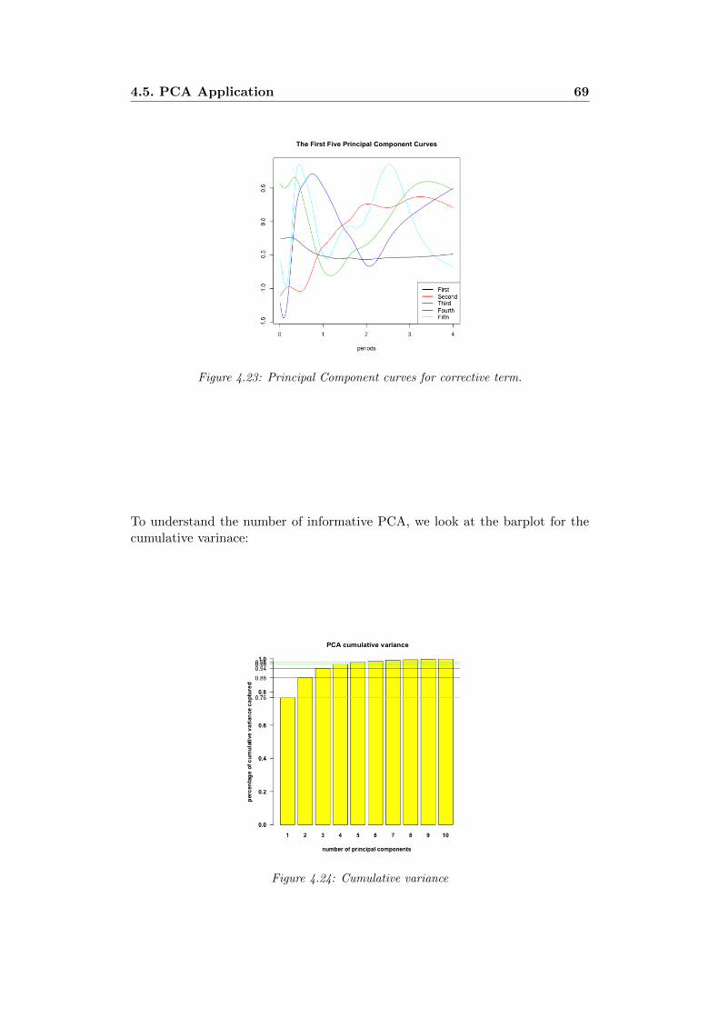
4.5. PCA Application 69
Figure 4.23: Principal Component curves for corrective term.
To understand the number of informative PCA, we look at the barplot for thecumulative varinace:
Figure 4.24: Cumulative variance

70Chapter 4. Functional geostatistics for the joint analysis of intensity
measures over a range of periods
Figure 4.25: Boxplot of scores
Here, the right number of functions for the basis could be greater than five.Of course, we know that if we increase the number of functional directions, weget a better approximation but, as we will see in the next section, it is crucial toemploy only the minimum number of informative principal directions to improvethe computational performance. In the Figure 4.26 we compare the originalsmoothing splines and their projections by employing PCA with five scores.
Figure 4.26: Original smoothing spline and smoothing spline projected.
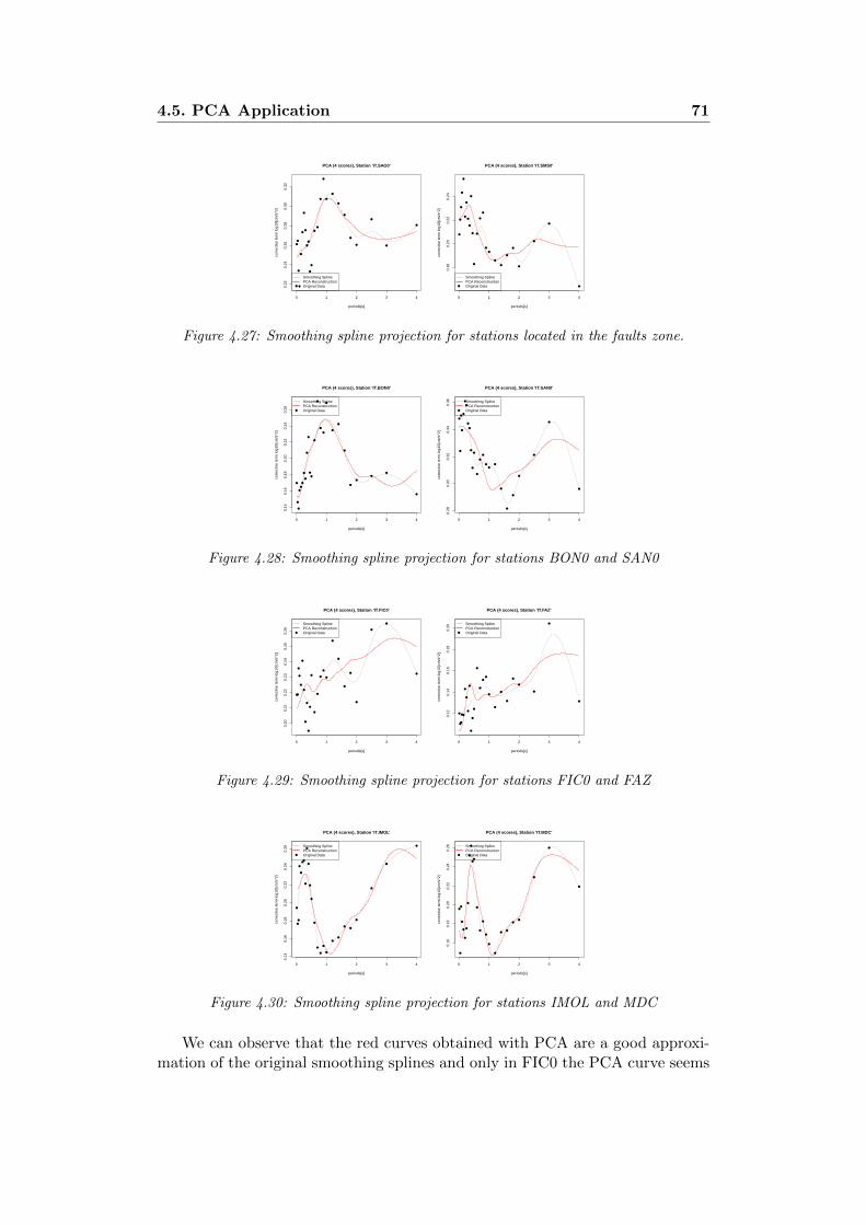
4.5. PCA Application 71
0 1 2 3 4
0.22
0.24
0.26
0.28
0.30
0.32
PCA (4 scores), Station 'IT.SAG0'
periods[s]
corr
ectiv
e te
rm lo
g10[
cm/s
^2]
●
●
●
●
●
●
●
●
●
●
●
●
●
●
●
●
●
●
●
●
●
●
●
●
●
Smoothing SplinePCA ReconstructionOriginal Data●
0 1 2 3 4
0.18
0.20
0.22
0.24
PCA (4 scores), Station 'IT.SMS0'
periods[s]
corr
ectiv
e te
rm lo
g10[
cm/s
^2]
●
●
●
●
●
●
●
●
●
●
●
●
●
●
●
●
●
●
●
●
●
●
●
●
●
Smoothing SplinePCA ReconstructionOriginal Data●
Figure 4.27: Smoothing spline projection for stations located in the faults zone.
0 1 2 3 4
0.14
0.16
0.18
0.20
0.22
0.24
0.26
PCA (4 scores), Station 'IT.BON0'
periods[s]
corr
ectiv
e te
rm lo
g10[
cm/s
^2]
●
●
●
●
●
●
●
●
●
●
●
●
●
●
●
●
●
●
●
●
●
●
●
●
●
Smoothing SplinePCA ReconstructionOriginal Data●
0 1 2 3 4
0.28
0.30
0.32
0.34
0.36
PCA (4 scores), Station 'IT.SAN0'
periods[s]
corr
ectiv
e te
rm lo
g10[
cm/s
^2]
●
●
●
●
●
●
●
●
●
●
●
●
●
●
●
●
●
●
●
●
●
●
●
●
●
Smoothing SplinePCA ReconstructionOriginal Data●
Figure 4.28: Smoothing spline projection for stations BON0 and SAN0
0 1 2 3 4
0.20
0.21
0.22
0.23
0.24
0.25
0.26
PCA (4 scores), Station 'IT.FIC0'
periods[s]
corr
ectiv
e te
rm lo
g10[
cm/s
^2]
●●
●
●
●
●
●
●
●
●
●
●
●
●
●
●
●
●
●
●
●
●
●
●
●
Smoothing SplinePCA ReconstructionOriginal Data●
0 1 2 3 4
0.12
0.14
0.16
0.18
0.20
PCA (4 scores), Station 'IT.FAZ'
periods[s]
corr
ectiv
e te
rm lo
g10[
cm/s
^2]
●
●●
● ●
●
●
●
●
●
●
●
●
●
●
●
●
●
●
●
●
●
●
●
●
Smoothing SplinePCA ReconstructionOriginal Data●
Figure 4.29: Smoothing spline projection for stations FIC0 and FAZ
0 1 2 3 4
0.14
0.16
0.18
0.20
0.22
0.24
0.26
PCA (4 scores), Station 'IT.IMOL'
periods[s]
corr
ectiv
e te
rm lo
g10[
cm/s
^2]
●
●
●
●
●
●●
●
●
●
●
●
●
●
●
●
●
●
●
●●
●
●
●
●Smoothing SplinePCA ReconstructionOriginal Data●
0 1 2 3 4
0.16
0.18
0.20
0.22
0.24
0.26
PCA (4 scores), Station 'IT.MDC'
periods[s]
corr
ectiv
e te
rm lo
g10[
cm/s
^2]
●
●
●
●
●
●
●
●
●
●
●
●
●
●
●
●
●
●
●●
●
●
●
●
●
Smoothing SplinePCA ReconstructionOriginal Data●
Figure 4.30: Smoothing spline projection for stations IMOL and MDC
We can observe that the red curves obtained with PCA are a good approxi-mation of the original smoothing splines and only in FIC0 the PCA curve seems

72Chapter 4. Functional geostatistics for the joint analysis of intensity
measures over a range of periods
to have a different behaviour when the concavity of the function changes sud-dently. By adding scores, we are able to catch this behaviour. However, in orderto avoid the overfitting, we don’t want to employ models too complex since ourdata could be affected by noise and models with a large number of degree offreedom would fit that noise.
4.6 Multivariate Sequential Simulation
Through the FPCA we are able to create a bijection between the smoothingspline gs in station s and a vector of scores
scs = (sc1,s, sc2,s, sc3,s, sc4,s)′
where the i-th score represents the projection of the curves on the i-th functionalprincipal direction fi:
sc1,s =∫gsf1 sc2,s =
∫gsf2 sc3,s =
∫gsf3 sc4,s =
∫gsf4
In this way, instead of working with functions, we can reduce the dimensionalityof the problem and we can work with vectors of 4 components. Given the71 vectors of 4 scores, we would like to simulate, in a new location s0, thecorresponding vector of four scores scs0 = (sc1,s0 , sc2,s0 , sc3,s0 , sc4,s0) and thenby a linear combination of the vector and the FPCA basis {f1, f2, f3, f4} we canreconstruct the shape of the function of the corrective term versus the period inthat location
gs0 =
4∑i=1
fisci,s0 (4.36)
The conditional simulation requires to estimate the covariance matrix of themultivariate random field. The covariance can be recovered from the samplevariogram, as in the scalar random field, but in the multivariate framework weneed to introduce the concepts of the cross-covariance and the cross-variogram.First we can observe that, by construction, each of the four score random fieldhas zero mean.The cross-covariance functions (Chiles et Delfiner,1999) of a p-dimensional(inour case p=4) stationary random field Z(x) = (Z1(x), ..., .Zp(x))′ with meanvector m(x) = (m1(x), ...,mp(x))′(in our case m(x) = 0 ∀x) are defined by
Ci,j(h) = E[Zi(x)−mi][Zj(x+ h)−mj ] (4.37)
If we permute the variables, we get another cross-covariance
E[Zj(x)Zi(x+ h)] = Cji(h) (4.38)
note also that
Cij(h) = E[Zi(x)Zj(x+ h)] = E[Zj(x+ h)Zi(x)] = Cji(−h) (4.39)
and in generalCij(−h) 6= Cij(h) (4.40)

4.6. Multivariate Sequential Simulation 73
The total covariance matrix will have the form:
Σ =
C11 C12 .. C1p
C21 C22 .. C2p
..Cp1 Cp2 .. Cpp
(4.41)
where Cii collects the covariance of the i-th component of the vector in differentlocations. In the univariate random field case
Σ = C11 (4.42)
As previously defined the Cij terms collects the cross-covariance of the i-j com-ponents of the vector at different locations.As we did in the univariate case, first we create the sample variogram, secondlywe fit the sample variogram with a valid model and finally we retrieve the co-variance structure of the field. To construct the Cross-covariance we use theCross-variogram. Under the condition E[Zi(x+ h)−Zi(x)] = 0 for i = 1, ., pthe cross-variogram, introduced by Matheron (1965), has the form
γ12(h) = E[(Z1(u+ h)− Z1(u))(Z2(u+ h)− Z2(u))] (4.43)
and the relationship with the cross-covariance is
γi,j(h) = Ci,j(0)− 1
2[Ci,j(h) + Ci,j(−h)] (4.44)
4.6.1 Application for Correttive Term and σ0,sr
We compute the sample cross-variogram and we fit the exponential model. Forthe corrective term, we use a basis of four principal components curves so wehave a vector random field of four components. Instead, for σ0,sr, we use fivescores:
Figure 4.31: Corrective term(on the left) and σ0,sr (on the right) variograms and cross-variograms fitted with the exponential model.

74Chapter 4. Functional geostatistics for the joint analysis of intensity
measures over a range of periods
From the variogram we estimate the cross-covariance and performs conditionalsimulation of the vectors on the grid of 70000 points.From the simulated scores, we can reconstruct the curves in all the 70000 lo-cations and from each locations we can find from the curves the value of thePGA and the corrective term/σ0,sr valutated at T = 4s. Both for σ0, sr and thecorrective term, we compare the simulations for PGA and T = 4s on the wholegrid and on the faults.
Figure 4.32: Sequential simulation of corrective term PGA(on the left) and T = 4s (onthe right).
640 660 680 700 720 740
4920
4940
4960
4980
5000
5020
PCA Corrective Term−PGA log10[cm/s^2]
Longitude, UTM[Km]
Latit
ude,
UT
M[k
m]
−0.5
0.0
0.5
1.0
FaultsA−A'StationsEpicenters
640 660 680 700 720 740
4920
4940
4960
4980
5000
5020
PCA Corrective Term−T=4[s] log10[cm/s^2]
Longitude, UTM[Km]
Latit
ude,
UT
M[k
m]
−0.5
0.0
0.5
1.0
FaultsA−A'StationsEpicenters
Figure 4.33: Sequential simulation of corrective term PGA (on the left) and T = 4s (onthe right), zoom on the faults.
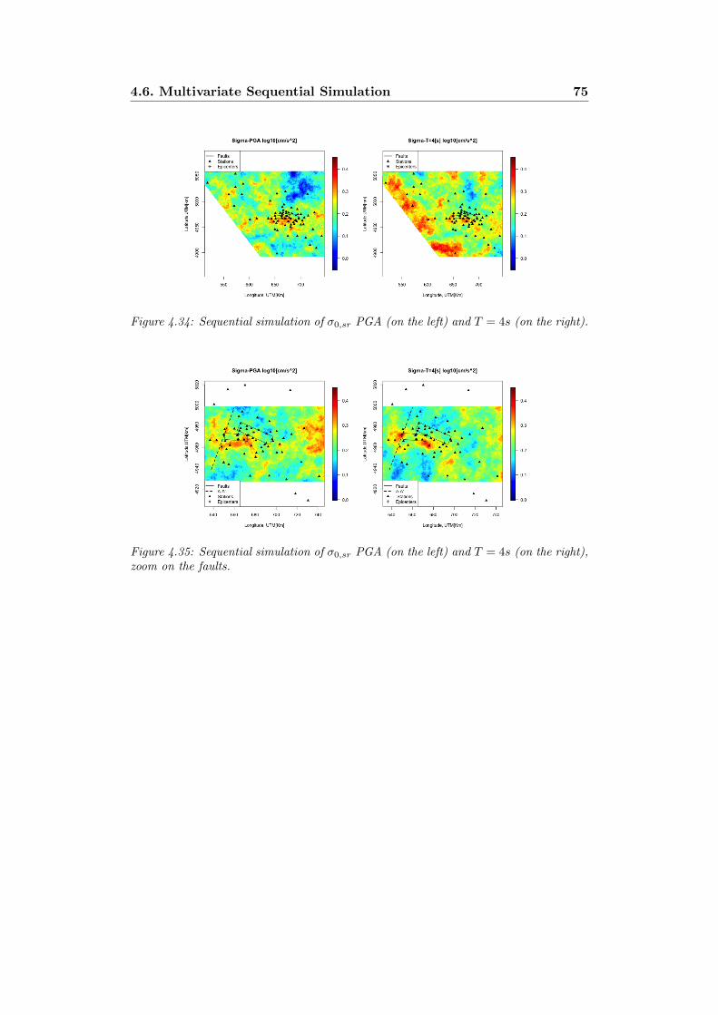
4.6. Multivariate Sequential Simulation 75
Figure 4.34: Sequential simulation of σ0,sr PGA (on the left) and T = 4s (on the right).
Figure 4.35: Sequential simulation of σ0,sr PGA (on the left) and T = 4s (on the right),zoom on the faults.

76Chapter 4. Functional geostatistics for the joint analysis of intensity
measures over a range of periods

Chapter 5
Model validation and testing
5.1 Model Comparison
In the previous chapter we have computed the kriging prediction for both thecorrective term and σ0,sr at PGA and SA(T=4s) through the univariate ap-proach and the functional one.Now we want to compare the two models through the leave one out cross vali-dation.We report the performances of the two models adopting as metric the meansquare error (MSE) and we take into account also its variance (VAR).
MSE =1
N
∑s∈S
(Zs − Zs)2 (5.1)
V AR =1
N − 1
∑s∈S
((Zs − Zs)2 −MSE)2 (5.2)
Where S is the set of the stations.The performances of the univariate approach in terms of MSE are reported inTable 5.1. and its variance in Table 5.2
σ0,sr corrective term
PGA 0.0027 0.0269
T = 4[s] 0.0023 0.1496
Table 5.1: Univariate geostatistics performances, MSE.
σ0,sr corrective term
PGA 9.9 ∗ 10−6 0.00144
T = 4[s] 1.99 ∗ 10−5 0.628
Table 5.2: Univariate geostatistics performances, VAR
77

78 Chapter 5. Model validation and testing
The performances of the functional approach in terms of MSE are reported inTable 5.3 and its variance in Table 5.4.
σ0,sr corrective term
PGA 0.0025 0.05287
T = 4[s] 0.0026 0.0281
Table 5.3: Functional geostatisctics performances, MSE.
σ0,sr corrective term
PGA 1.5 ∗ 10−5 0.005
T = 4[s] 2.3 ∗ 10−5 0.0029
Table 5.4: Functional geostatistics performances, VAR.
We can observe that the two methods have comparable MSE when they areapplied to σ0,sr. For the corrective term, the MSE of the univariate approach forPGA is slightly better than the MSE of the functional approach. Conversely thefunctional approach shows a better MSE in case T = 4s in which the univariaterandom field of the corrective term is assumed to have drift non-constant in space.Nevertheless, we have to consider that only the functional approach provides theprediction and the stocastic simulation of the whole spectrum and not only forthis specific intensity measures (PGA and T = 4s).
5.2 Test
A leave-one-out cross-validation analysis highlights that modeling the spatialcovariance of the corrective term for PGA with the univariate and the functionalstatistics provides very similar results while the best model in the case of T=4sis the functional one. We can compute the shaking fields based on the GMPEprediction for the first main event of the Emilia sequence (2012-05-20, MW =6.1).
For fifty five stations we have the values of PGA and SA(T = 4). By computingthe MSE between the intensity measures observed in the aforementioned stationsand the closest point of a grid, defined as a collection of 70000 points whereour GMPE has been evaluated, we test the prediction performance of modelsobtained with:
• functional kriging based on the simple cokriging of the FPCA scores (seeChapter 4) (evaluated in the PGA and T = 4s).
• ordinary kriging for the univariate case PGA (see chapter 3).
In Table 5.5 we report the MSE values for the GMPE and for a model obtainedby adding the GMPE to the kriging prediction of the PGA computed with an

5.2. Test 79
univariate approach. MSE2 in table 5.5 is computed taking into account all thestations available, the MSE1 doesn’t consider the station closest to the fault.
GMPE[cm/s2] Model [cm/s2]
MSE1 59.82 56.93
MSE2 171.24 661.51
Table 5.5: MSE for the model (univariate) and GMPE at PGA.
The station closest to the fault is dramatically overestimated by the two modelsand it significantly changes the value of the MSE. In the Table 5.6 we reportthe MSE for a predictive model of PGA, obtained by adding the GMPE tothe kriging prediction of the PGA computed with the functional geostatisticsapproach. The model has a lower MSE in both the cases. We still observe that
GMPE[cm/s2] Model[cm/s2]
MSE1 59.82 56.32
MSE2 171.24 101.56
Table 5.6: MSE for the model (functional) and GMPE at PGA.
if we include the station closest to the fault, the MSE dramatically increases.
In table 5.7 we compare the GMPE predictions of SA(T=4s) and the predic-tions of a model obtained by adding the GMPE to the kriging prediction of theSA(T=4s) computed with the functional geostatistics approach,. The MSE1 Intable 5.7 is obtained by taking into account all the stations in the region andwe observe that the GMPE for SA(T=4s) has better performance. The stationclose the fault is well estimated by both the GMPE and the model, therefore wedon’t need to report MSE2.
GMPE[cm/s2] Model[cm/s2]
MSE1 16.22 21.56
Table 5.7: MSE for the model(functional) and for the GMPE at T = 4s.
Finally, we report the simulated shaking fields, for the first main event of theEmilia sequence computed as the sum of the GMPE, the corrective term sim-ulated through the functional approach and a realization of a gaussian randomfield uncorrelated in space with zero mean and variance σ0,sr. Also the varianceσ0,sr has been simulated through the functional approach. We report in Figure5.1 the simulated shaking fields for PGA and for SA(T=4s) and in Figure 5.2,5.3 on the left panel, the GMPE and, on the right panel, the simulation of theshaking fields, with the colour scale saturated in the upper part, in order tocompare it to the GMPE.

80 Chapter 5. Model validation and testing
550 600 650 700
4900
4950
5000
5050
Shaking Field Simulation PGA [cm/s^2]
Longitudine, UTM[Km]
Latit
udin
e,U
TM
[km
]
0
200
400
600
800
1000
FaultsStationsEpicenters
550 600 650 700
4900
4950
5000
5050
Shaking Field Simulation T=4s [cm/s^2]
Longitudine, UTM[Km]
Latit
udin
e,U
TM
[km
]
0
20
40
60
80
FaultsStationsEpicenters
Figure 5.1: Shaking fields for PGA and SA(T=4s).
550 600 650 700
4900
4950
5000
5050
GMPE PGA [cm/s^2]
Longitudine, UTM[Km]
Latit
udin
e,U
TM
[km
]
100
200
300
400
FaultsStationsEpicenters
550 600 650 700
4900
4950
5000
5050
Shaking Field Simulation PGA [cm/s^2]
Longitudine, UTM[Km]
Latit
udin
e,U
TM
[km
]
0
100
200
300
400
FaultsStationsEpicenters
Figure 5.2: GMPE and shaking field for PGA, same scale.
550 600 650 700
4900
4950
5000
5050
GMPE T=4s [cm/s^2]
Longitudine, UTM[Km]
Latit
udin
e,U
TM
[km
]
10
20
30
40
FaultsStationsEpicenters
550 600 650 700
4900
4950
5000
5050
Shaking Field Simulation T=4s [cm/s^2]
Longitudine, UTM[Km]
Latit
udin
e,U
TM
[km
]
0
10
20
30
40
FaultsStationsEpicenters
Figure 5.3: GMPE and shaking field for SA(T=4s), same scale.
We can observe that the simulation of the shaking fields presents greater valuesthan the ones of the GMPE in the fault zone, where the epicenter of the event islocated and the GMPE assigns a constant value to all the points. For SA(T=4s)we can observe a strong amplification in the area of the Appenninies that couldbe consequence of complex site effects due to the presence of surface waves.
Chapter 6
Conclusion
The corrective term and σ0,sr for PGA and SA(T = 4s) have been investigatedin order to study the spatial correlation and to predict their value in new loca-tions.First, through the univariate approach, it has been observed that the correctiveterm of PGA becomes uncorrelated faster than the one of SA(T = 4s). The sta-tistical results have been evaluated also considering the features of ground motioncharacterization specific for the area of study. S waves, which are generated bythe trapping and conversion of the body waves in the thick sedimentary cover,dominate the seismic signals at periods longer than two seconds and determinethe increase of correlation distance at long periods.Since SA is function of the period of oscillation T, it has been possible to repre-sent our data as a curve and to study their spatial covariance taking into accountthe inter-period correlation through FDA methods. We have approximated datathrough smoothing spline and we have recreated the curves for the correctiveterm of the GMPE and σ0,sr through the prediction and the simulation of thescores calculated by the Functional Principal Components Analysis. In this way,we have reproduced possible shaking scenarios for the corrective term and σ0,sr
of PGA and SA(T = 4s). The prediction performance of the univariate and thefunctional approaches have been compared by means of cross-validation.Cross validation indicates that the univariate and the functional approach havesimilar results for σ0,sr that don’t depend on the period. For what concerns thecorrective terms, the univariate approach presents slightly better results at lowperiods while the functional approach presents much better results for SA(T=4s).This difference in performance could be connected to the drift estimation prob-lem of the corrective term when we apply the univariate approach at T=4s. Inconclusion, considering both the results and the availability of joint stochasticsimulation of several periods, the functional approach is the best one.
81

82 Chapter 6. Conclusion

Bibliography
Abrahamson, N., Youngs, R.R. (1992). A stable algorithm for regression anal-yses using the random effects model. Bulletin of the Seismological Society ofAmerica, 82:505-510.
Al-Atik, L., N.A. Abrahamson, J.J. Bommer, F. Scherbaum, F. Cotton andN. Kuehn (2010). The variability of ground-motion prediction models and itscomponents. Seismological Research Letters, 81(5):794–801.
Anderson, J.G.and Brune J.N. (1999). Probabilistic seismic hazard assessmentwithout the ergodic assumption. Seismological Research Letters, 70:19–28.
Bigi, G., Bonardi, G., Catalano, R., Cosentino, D., Lentini, F., Parotto, M.,Sartori, R., Scandone, P., Turco, E. (1992). Structural model of Italy 1:500,000,CNR Progetto Finalizzato Geodinamica.
Bivand, R.S., Pebesma, E., Gomez-Rubio, V. (2013). Applied Spatial Data Anal-ysis with R.
Boccaletti, M., Bonini, M., Corti, G., Gasperini, P., Martelli, L., Piccardi, L.,Severi, P., Vannucci, G. (2004). Seismotectonic map of the Emilia Romagna Re-gion, Emial-Romagna Region - SGSS and CNR-IGC, S.EL.CA Florence
Boore, D.M, JoYner, W.B, Fumal, T.E. (1993). Estimation of response spectraand peak accelerations from Western North American earthquakes: an interimreport.
Bradley, B.A. (2014). Site-specific and spatially-distributed ground-motion in-tensity estimation in the 2010–2011 Canterbury earthquakes. Soil Dynamics andEarthquake Engineering, 61-62, 83-91.
Bragato, P.L., Vuan, A., Massa, M., Sarao, A. (2011). Moho Reflection Effects inthe Po Plain (Northern Italy) Observed from Instrumental and Intensity Data.Bulletin of the Seismological Society of America, 5:2142-2152.
Chiles, J-P. and Delfiner, P. (1999). Geostatistics: Modeling Spatial Uncertainty.
83
84 BIBLIOGRAPHY
Cressie, N. (1993). Statistics for Spatial Data.
Delicado, P., Giraldo, R., Comas, C., Mateu, J. (2010). Statistics for spatialfunctional data. Environmetrics, 21(3-4):224-239.
Douglas, J. (2003). Earthquake ground motion estimation using strong-motionrecords: a review of equations for the estimation of peak ground accelerationand response spectral ordinates. Earth-Science Reviews, 61:43-104.
Goda, K. and Atkinson, G. M. (2010). Intraevent Spatial Correlation of Ground-Motion Parameters Using SK-net Data. Bulletin of the Seismological Society ofAmerica, 100(1):3055–3067.
Goda, K. and Hong, H. P. (2008). Spatial Correlation of Peak Ground Mo-tions and Response Spectra. Bulletin of the Seismological Society of America,98(1):354–365.
Jayaram, N. and Baker, J.W. (2010). Considering Spatial Correlation in Mixed-Effects Regression and the Impact on Ground-Motion Models. Bulletin of theSeismological Society of America, 100:3295–3303.
Lanzano, G., D’Amico, M., Felicetta, C., Puglia, R., Luzi, L., Pacor, F., Bindi,D. (2016). Ground motion prediction equations for region specific probabilis-tic seismic hazard analysis. Bulletin of the Seismological Society of America,106(1):73–92.
Lanzano, G., Pacor, F., Luzi, L., D’Amico, M., Puglia, R., Felicetta, C. (2017).Systematic source, path and site effects on ground motion variability: the casestudy of Northern Italy. Bulletin of Earthquake Engineering, 15(11):4563–4583.
Lin, P.S., Chiou, B., Abrahamson, N., Walling, M., Lee, C.T., Cheng, C.T.(2011). Repeatable source, site, and path effects on the standard deviation forempirical ground-motion prediction models. Bulletin of the Seismolological So-ciety of America, 101:2281–2295.
Loth, C. and Baker, J.W. (2012). A spatial cross-correlation model for groundmotion spectral accelerations at multiple periods. Earthquake Engineering andStructural Dynamics, 42(3):397–417.
Luzi, L., Pacor, F., Ameri, G., Puglia, R., Burrato, P., Massa, M., Augliera, P.,Franceschina, G., Lovati, S., Castro, R. (2013). Overview on the strong-motiondata recorded during the May-June 2012 Emilia Seismic Sequence. SeismologicalResearch Letters, 84(4):629-644.
Luzi, L., Puglia, R., Russo, E., D’Amico, M., Felicetta, C., Pacor, F., Lanzano,G., Ceken, U., Clinton, J., Costa, G. et al. (2016). The Engineering strong-

BIBLIOGRAPHY 85
motion database: a platform to access Pan-European accelerometric data. Seis-mological Research Letters, 87(4):987–997.
Matheron, G. (1965). Principles of geostatistics. Econ. Geol. 58:1246-1266.
Meletti, C., Galadini, F., Valensise, G., Stucchi, M., Basili, R., Barba, S., Van-nucci, G., Boschi, E., (2008). A seismic source zone model for the seismic hazardassessment of the Italian territory. Tectonophysics, 450(1):85–108.
Menafoglio, A., Guadagnini, A., Secchi, P. (2016). Stochastic Simulation of SoilParticle-Size Curves in Heterogeneous Aquifer Systems through a Bayes spaceapproach. Water Resources Research, 52:5708-5726.
Menafoglio, A., Secchi, P. (2017). Statistical analysis of complex and spatiallydependent data: a review of Object Oriented Spatial Statistics. European Jour-nal of Operational Research, 258(2):401-410.
Nerini, D., Monestiez, P., Mante, C. (2016). Cokriking for spatial functionaldata. Journal of Multivariate Analysis, 101(2):409-418.
Paolucci, R., Mazzieri, I., Smerzini, C. (2015). Anatomy of strong ground mo-tion: near-source records and 3D physics-based numerical simulations of the Mw6.0 May 29 2012 Po Plain earthquake, Italy, 203:2001–2020.
Pacor, F., Paolucci, R., Luzi, L., Sabetta, F., Spinelli, A., Gorini, A., Nicoletti,M., Marcucci, S., Filippi, L., Dolce, M. (2011). Overview of the Italian strongmotion database ITACA 1.0. Bulletin of Earthquake Engineering, 9:1723–1739.
Park, J., Bazzurro, P. and Baker, J.W. (2007). Modeling spatial correlationof ground motion Intensity Measures for regional seismic hazard and portfolioloss estimation. Applications of Statistics and Probability in Civil Engineering,1-8.
Ramsay, J.O. and Silverman, B.W. (2005). Functional data analysis.
Rodriguez-Marek, A., Cotton, F., Abrahamson, N., Akkar, S., Al Atik, L.,Edwards, B., Montalva, G.A., Dawood, H.(2013). A model for single-stationstandard deviation using data from various tectonic regions. Bulletin of the Seis-molological Society of America, 103:3149–3163.
Verros, S.A., Wald, D.J., Worden, C.B., Hearne, Ganesh, M. (2017). Computingspatial correlation of ground motion intensities for ShakeMap. Computers Geo-sciences, 99:145-154.
Villani, M. and Abrahamson, N. (2015). Repeatable site and path effects onthe ground-motion sigma based on empirical data from Southern California and

86 BIBLIOGRAPHY
simulated waveforms from the CyberShake platform. Bulletin of the Seismolo-logical Society of America, 105(5):2681–2695.
Zerva A. and Zervas, V. (2002). Spatial variation of seismic ground motions:An overview. Applied Mechanics Reviews, 55(3):271-297.